
Recovery and Restoration of the Seagrass Halodule wrightii after ...
102
RECOVERY AND RESTORATION OF THE SEAGRASS HALODULE WRIGHTII AFTER BOAT PROPELLER SCAR DAMAGE IN A POLE-TROLL ZONE IN MOSQUITO LAGOON, FLORIDA by KATHERINE RUTH GRABLOW B.S. University of Central Florida, 2006 A thesis submitted in partial fulfillment of the requirements for the degree of Master of Science in the Department of Biology in the College of Sciences at the University of Central Florida Orlando, FL Fall 2008
Transcript of Recovery and Restoration of the Seagrass Halodule wrightii after ...

RECOVERY AND RESTORATION OF THE SEAGRASS HALODULE WRIGHTII AFTER
BOAT PROPELLER SCAR DAMAGE IN A POLE-TROLL ZONE IN MOSQUITO
LAGOON, FLORIDA
by
KATHERINE RUTH GRABLOW
B.S. University of Central Florida, 2006
A thesis submitted in partial fulfillment of the requirements
for the degree of Master of Science
in the Department of Biology
in the College of Sciences
at the University of Central Florida
Orlando, FL
Fall 2008

ii
ABSTRACT
This study combined documentation of four boat propeller scar types in Halodule wrightii
seagrass beds in Mosquito Lagoon, Florida with manipulative field experiments to document scar
recovery times with and without restoration. Scar types ranged from the most severe scar type
(Type 1) with trench formation which had no roots or shoots in the trench, to the least severe
(Type 4) scars that had no depth, intact roots and shoots shorter than the surrounding canopy. For
110 measured existing scars, the frequency of each scar type was 56% for Type 1, 10% for Type 2,
7% for Type 3, and 27% for Type 4. In the first manipulative experiment, experimental scars were
created to document the natural recovery time of H. wrightii for each scar severity within one year.
Type 4 scars recovered to the control shoot density at 2 months, while Types 1, 2, and 3 scars did
not fully recover in one year. Mean estimated recovery for H. wrightii is expected in 25 months
for Type 1, and 19 months for Types 2 and 3. For the second manipulative experiment, three
restoration methods were tested on Type 1 scars over a 1 year period. Restoration methods
included: (1) planting H. wrightii in the scar trench, (2) filling the trench with sand, and (3) filling
with sand plus planting H. wrightii. There was complete mortality of all transplants at 2 months
and only 25% of scars retained fill sand after 1 year. With dense adjacent seagrass beds, natural
recovery was more successful than any of my restoration attempts. Thus, I suggest that managers
should concentrate on preventing seagrass destruction rather than restoration.

iii
To my husband Seth, and my family for all their help, love, and support.

iv
ACKNOWLEDGMENTS
Thank you Seth Grablow, Louis Brown, Molly Brown, Nicole Martucci, Julia Leissing,
Andrea Barber, Jason Ledgard, Hayley Ashworth, Iris Howell, Matthew Mitchell, Laurie Holliday,
Christy Akers, Shannon Hackett, Kristen Kneifl, Ethan Nash, Elizabeth Bourassa, Gisela Harper,
Justin Bridges, Rachel Odom, Wei Yuan, Sasha Brodsky, the Student Conservation Association
interns, and Canaveral National Seashore Physical Labor Crew for helping set up and measure the
experiment in the field. Thank you Linda Walters, David Jenkins, Robert Virnstein, Troy Rice,
Robert Day, Lori Morris, Lauren Hall, John Stiner, and Mike Legare, for your guidance, support
and encouragement! Thank you to the University of Central Florida Graduate Studies Research
and Mentoring Fellowship, Department of Biology, Indian River Lagoon National Estuary
Program, St. Johns River Water Management District, Garden Club of America, and International
Women’s Fishing Association for supporting and funding this project.

v
TABLE OF CONTENTS
CHAPTER 1: GENERAL INTRODUCTION ........................................................................... 1
CHAPTER 2: BASELINE SCAR MEASUREMENTS ............................................................ 6
METHODS .................................................................................................................................... 6 Study organism ....................................................................................................................... 6 Study area................................................................................................................................ 7 Measurements of existing propeller scars ............................................................................... 8 Intra-scar measurements ......................................................................................................... 9
Sediment analyses ................................................................................................................... 9 Statistical analyses ................................................................................................................ 10
RESULTS .................................................................................................................................... 11 Scar severity categories......................................................................................................... 11 General scar measurements................................................................................................... 12 Intra-scar measurements ....................................................................................................... 13
Scar sediment analysis .......................................................................................................... 13 DISCUSSION ............................................................................................................................... 14
CHAPTER 3: MANIPULATIVE EXPERIMENTS ............................................................... 18
METHODS .................................................................................................................................. 18 Study area.............................................................................................................................. 18
Layout and monitoring of experiments ................................................................................. 19 Natural recovery of seagrass in experimental propeller scars .............................................. 20
Restoration of experimental propeller scars ......................................................................... 21
Sediment core analysis .......................................................................................................... 23
RESULTS .................................................................................................................................... 23 Site consistency ..................................................................................................................... 23
Natural recovery experiment................................................................................................. 24 Seasonal variations in natural recovery ................................................................................ 27 Restoration experiment ......................................................................................................... 28
Erosion observations ............................................................................................................. 29 DISCUSSION ............................................................................................................................... 31
Natural recovery.................................................................................................................... 31 Seagrass restoration .............................................................................................................. 31
Management recommendations ............................................................................................ 33 Restoration versus prevention ............................................................................................... 34
Future of seagrass in Mosquito Lagoon ................................................................................ 35
APPENDIX A: LIST OF FIGURES ......................................................................................... 37
APPENDIX B: LIST OF TABLES ........................................................................................... 75
LITERATURE CITED .............................................................................................................. 87

vi
LIST OF FIGURES
Figure 1: Map of experimental scar locations in the Pole-Troll Zone of Mosquito Lagoon,
Florida. Boundary of the Pole-Troll Zone is marked by a dotted line with black circles.
Channels include: the Atlantic Intercoastal Waterway (ICW) as a solid black line, and the
inner Pole-Troll Zone channels are dotted lines within the Pole-Troll Zone boundaries. .... 38
Figure 2: Halodule wrightii seagrass bed in Mosquito Lagoon, FL. ............................................ 39
Figure 3: Location of 110 propeller scars measured in Mosquito Lagoon, FL. Scar type is color
coded to show the frequency of each scar type. From this view, the entire range of
measured scars is demonstrated, however not all scars can be seen due to overlap. ............ 40
Figure 4: Canonical Discriminant Analysis classification of 110 propeller scars in Mosquito
Lagoon. Scars were sorted into four groups. Type 1 scars are white circles, Type 2 scars are
black squares, Type 3 scars are black triangles, and Type 4 scars are white diamonds. ...... 41
Figure 5: Scar types identified from measuring 110 scars in Mosquito Lagoon. Above diagram
simplifies what was seen in each of the photographs below................................................. 42
Figure 6: Frequency of scar types in Mosquito Lagoon (n = 110). .............................................. 42
Figure 7: Regression of Type 1 scar width versus scar depth. Scar Type 1 was used to show the
best correlation (r2 = 0.476, p < 0.001), because other scar types (2-4) did not have depth. 43
Figure 8: Mean percent of sediment grain size fractions and organic content per scar type.
Percent sediment fraction sizes are listed in order < 1mm is light grey cross hatch, 1 mm is
dark grey cross hatch, 2 mm is solid black, 5 mm is solid white, > 5mm is solid light grey,
and percent organic content is solid dark grey. Using a one-way ANOVA, only scar Type 1
and 4 were significantly different in all fraction sizes, and size < 1mm showed the greatest
difference. ............................................................................................................................. 44
Figure 9: Canonical Discriminant Analysis classification of 110 propeller scars sediment
fractions and distance measurements. Type 1 scars are white circles, Type 2 scars are black
squares, Type 3 scars are black triangles, and Type 4 scars are white diamonds. Sediment
types did not show a pattern in relation to distance. ............................................................. 45
Figure 10: Layout of one block of experimental scars. Each block was 18 x18 m and was divided
into 9 squares, of which only 8 had a scar treatment. A square was 6 x 6 m containing a
single scar treatment in the center. ........................................................................................ 46
Figure 11: Setup of a one set of treatments in a large grid (block). An 18 x 18 m perimeter was
marked off with yellow rope, and a PVC pole was placed every 6 m. Scars were created in
the center of each 6 x 6 m square and marked with a short PVC pole at each end. All PVC
grid poles were marked with a GPS location and then removed. After the scars were
created, only the 2 PVC scar markers remained to mark the ends of each scar. .................. 46

vii
Figure 12: PVC stake marking the end of an experimental scar. .................................................. 47
Figure 13: PVC plow 32 cm in diameter. Device used to make experimental propeller scars the
same width, depth, and scar slope angle. .............................................................................. 47
Figure 14: Arrow points to H. wrightii attached to garden staple with a twist tie in a scar filled
with sand. This is an eroded staple, making it is easier to see how H. wrightii was attached
with a red twist tie. ................................................................................................................ 48
Figure 15: Mean water temperature on sampling dates (± S.E.) at location of manipulative
experiments (n = 3). .............................................................................................................. 49
Figure 16: Mean salinity (± S.E.) at location of manipulative experiments on sampling dates (n =
3). .......................................................................................................................................... 49
Figure 17: Mean water clarity depth (± S.E.) at location of manipulative experiments on
sampling dates (n = 3). Maximum measurement possible using turbitdity tube was 60 cm.
............................................................................................................................................... 50
Figure 18: Mean water depth (± S.E.) of experimental scar locations of manipulative experiments
(n = 10). There were no significant differences of mean water depth among replicate blocks
(Kruskal-Wallis rank test p > 0.006). .................................................................................... 50
Figure 19: Mean surrounding scar H. wrightii density (± S.E.) per 25 x 25 cm area in
experimental scar replicate blocks. There were no significant differences among
surrounding densities in replicate blocks (Kruskal-Wallis rank test p > 0.006). .................. 51
Figure 20: Mean surrounding scar H. wrightii percent cover (± S.E.) per 25 x 25 cm area in
experimental scar replicate blocks. There were no significant differences among
surrounding H. wrightii mean percent cover in replicate blocks (Kruskal-Wallis rank test: p
> 0.006). ................................................................................................................................ 51
Figure 21: Mean surrounding scar H. wrightii canopy height (± S.E.) in experimental scar
replicate blocks. There were no significant differences among surrounding mean
surrounding canopy height in replicate blocks (Kruskal-Wallis rank test: p > 0.006). ........ 52
Figure 22: Natural recovery experimental scar H. wrightii shoot density per 25 x 25 cm area (±
S.E). Type 1 are black circles, Type 2 are white triangles, Type 3 are black squares, Type 4
are white diamonds, and control are black triangles. Measurements were analyzed with
Kruskal-Wallis rank test with a Bonferroni correction of p < 0.006. Treatments that were
significantly different on a single day are shown with different letters. ............................... 53
Figure 23: Natural recovery experimental scar H. wrightii percent cover per 25 x 25 cm area (±
S.E). Type 1 are black circles, Type 2 are white triangles, Type 3 are black squares, Type 4
are white diamonds, and control are black triangles. Measurements were analyzed with
Kruskal-Wallis rank test with a Bonferroni correction of p < 0.006. Treatments that were
significantly different on a single day are shown with different letters. ............................... 54

viii
Figure 24: Natural recovery experimental scar H. wrightii canopy height (± S.E). Type 1 are
black circles, Type 2 are white triangles, Type 3 are black squares, Type 4 are white
diamonds, and control are black triangles. Measurements were analyzed with Kruskal-
Wallis rank test with a Bonferroni correction of p < 0.006. Treatments that were
significantly different on a single day are shown with different letters. ............................... 55
Figure 25: Natural recovery experimental scar percent root cover per 25 x 25 cm area (± S.E).
Type 1 are black circles, Type 2 are white triangles, Type 3 are black squares, and Type 4
are white diamonds. Measurements were analyzed with Kruskal-Wallis rank test with a
Bonferroni correction of p < 0.006. Treatments that were significantly different on a single
day are shown with different letters. ..................................................................................... 56
Figure 26: Natural recovery experimental scar percent leaf litter cover per 25 x 25 cm area (±
S.E). Type 1 are black circles, Type 2 are white triangles, Type 3 are black squares, and
Type 4 are white diamonds. Measurements were analyzed with Kruskal-Wallis rank test
with a Bonferroni correction of p < 0.006. Treatments that were significantly different on a
single day are shown with different letters. .......................................................................... 57
Figure 27: Natural recovery experimental scar depth (± S.E). Type 1 are black circles, Type 2
are white triangles, Type 3 are black squares, and Type 4 are white diamonds.
Measurements were analyzed with Kruskal-Wallis rank test with a Bonferroni correction of
p < 0.006. Treatments that were significantly different on a single day are shown with
different letters. ..................................................................................................................... 58
Figure 28: Natural recovery experimental scar width (± S.E). Type 1 are black circles, Type 2
are white triangles, Type 3 are black squares, and Type 4 are white diamonds.
Measurements were analyzed with Kruskal-Wallis rank test with a Bonferroni correction of
p < 0.006. Treatments that were significantly different on a single day are shown with
different letters. ..................................................................................................................... 59
Figure 29: Natural recovery experimental scar slope angle density (± S.E). Type 1 are black
circles, Type 2 are white triangles, Type 3 are black squares, and Type 4 are white
diamonds. Measurements were analyzed with Kruskal-Wallis rank test with a Bonferroni
correction of p < 0.006. Treatments that were significantly different on a single day are
shown with different letters. ................................................................................................. 60
Figure 30: Natural recovery experiment mean percent sediment fractions (± S.E.) from before
scar creation and from within scars after 1 year (Kruskal-Wallis: p < 0.05). Bar sections are
labeled in order from left to right: initial, Type 1 (final), Type 2 (final), Type 3 (final), Type
4 (final), and control (final)................................................................................................... 61
Figure 31: Natural recovery experiment mean percent organic content (± S.E) from before scar
creation and from within scars after 1 year (Kruskal-Wallis: p < 0.05). .............................. 62
Figure 32: Restoration experimental scar H. wrightii density shoot density per 25 x 25 cm (±
S.E). Controls are white triangles, Type 1 are black circles, plant-only are black squares,
fill only are white diamonds, and plant and fill are black triangles. Measurements were
analyzed with Kruskal-Wallis rank test with a Bonferroni correction of p < 0.006.

ix
Treatments that were significantly different on a single day are shown with different letters.
............................................................................................................................................... 63
Figure 33: Restoration experimental scar H. wrightii percent cover per 25 x 25 cm area (± S.E).
Control are white triangles, Type 1 are black circles, plant-only are black squares, fill only
are white diamonds, and plant and fill are black triangles. Measurements were analyzed
with Kruskal-Wallis rank test with a Bonferroni correction of p < 0.006. Treatments that
were significantly different on a single day are shown with different letters. ...................... 64
Figure 34: Restoration experimental scar H. wrightii canopy height (± S.E). Control are white
triangles, Type 1 are black circles, plant-only are black squares, fill only are white
diamonds, and plant and fill are black triangles. Measurements were analyzed with
Kruskal-Wallis rank test with a Bonferroni correction of p < 0.006. Treatments that were
significantly different on a single day are shown with different letters. ............................... 65
Figure 35: Restoration experimental scar percent root cover per 25 x 25 cm area (± S.E). Type 1
are black circles, plant-only are white triangles, fill only are black squares, and plant and fill
are white diamonds. Measurements were analyzed with Kruskal-Wallis rank test with a
Bonferroni correction of p < 0.006. Treatments that were significantly different on a single
day are shown with different letters. ..................................................................................... 66
Figure 36: Restoration experimental scar percent leaf litter cover per 25 x 25 cm area (± S.E).
Type 1 are black circles, plant-only are white triangles, fill only are black squares, and plant
and fill are white diamonds. Measurements were analyzed with Kruskal-Wallis rank test
with a Bonferroni correction of p < 0.006. Treatments that were significantly different on a
single day are shown with different letters. .......................................................................... 67
Figure 37: Restoration experimental scar depth (± S.E). Control are white triangles, Type 1 are
black circles, plant-only are black squares, fill only are white diamonds, and plant and fill
are black triangles. Measurements were analyzed with Kruskal-Wallis rank test with a
Bonferroni correction of p < 0.006. Treatments that were significantly different on a single
day are shown with different letters. ..................................................................................... 68
Figure 38: Restoration experimental scar width (± S.E). Control are white triangles, Type 1 are
black circles, plant-only are black squares, fill only are white diamonds, and plant and fill
are black triangles. Measurements were analyzed with Kruskal-Wallis rank test with a
Bonferroni correction of p < 0.006. Treatments that were significantly different on a single
day are shown with different letters. ..................................................................................... 69
Figure 39: Restoration experimental scar slope angle density (± S.E). Control are white
triangles, Type 1 are black circles, plant-only are black squares, fill only are white
diamonds, and plant and fill are black triangles. Measurements were analyzed with
Kruskal-Wallis rank test with a Bonferroni correction of p < 0.006. Treatments that were
significantly different on a single day are shown with different letters. ............................... 70
Figure 40: Restoration experiment mean percent sediment fractions (± S.E.) from before scar
creation and from within scars after 1 year (Kruskal-Wallis: p < 0.05). Bar sections are

x
labeled in order from left to right: initial, control (final), Type 1 (final), plant only (final),
fill only (final), and plant and fill (final). .............................................................................. 71
Figure 41: Restoration experiment mean percent organic content (± S.E) from before scar
creation and from within scars after 1 year (Kruskal-Wallis: p < 0.05). .............................. 72
Figure 42: Types of erosion observed in experimental scars: A) holes, B) washouts, and C) sand
patches. The black rectangle represents the original scar dimensions, brown is bare
sediment, dark brown represents depth, and the green represents seagrass. ......................... 73
Figure 43: Bioturbation caused by a stingray. Stingray created a hole and unburied a row of
Halodule wrightii transplants on staples, then left behind a pile of feces. In the left picture
the arrow points to a close-up of excrement pile in hole, and in right picture the arrow points
to a close up of the eroded staples next to the excrement pile. ............................................. 73
Figure 44: Boater illegally using main engine motor in Pole-Troll Zone and running directly over
the experiment site. ............................................................................................................... 74
Figure 45: This PVC pole marking an experimental scar that was hit by main engine boat motor
in less than 0.5 m of water. ................................................................................................... 74

xi
LIST OF TABLES
Table 1: Previous studies documenting existing and experimental propeller scar damage and
recovery of seagrasses. Unavailable information was denoted with a dash, and recovery
times that included a restoration method were denoted with an asterisk. ............................. 75
Table 2: Canonical Discriminant Analysis results classifying 110 propeller scar measurements
into four groups. Table shows the percentage of scars correctly classified according to the
most important predictor variables: shoot density, scar depth, scar % root cover, and scar
canopy height. ....................................................................................................................... 76
Table 3: Mean scar measurements (± S.E.) for each scar type from 110 scars. ........................... 76
Table 4: Mean scar density measurements (± S.E.) per 25 x 25 cm area for each scar type from
110 scars. ............................................................................................................................... 77
Table 5: Canonical Discriminant Analysis results from classifying sediment fractions of 110
scars. This table shows the percentage of scars correctly classified according to original
identifications. Sediment fractions were not a good predictor of scar types. ...................... 77
Table 6: Mean experimental scar measurements (± S.E.) for scar Types 1-4 and control in natural
recovery experiment. Measurements were taken eight times from August 2007 through
August 2008. ......................................................................................................................... 78
Table 7: Kruskal-Wallis test for mean differences in measurements among scar types in natural
recovery experiment. Since tests were repeated eight times (once for each time period), the
significance level was corrected to p = 0.006 using the Bonferroni method. ....................... 81
Table 8: Mean experimental scar measurements (± S.E.) for three restoration treatments, and
Type 1 scar control in restoration experiment. Measurements were taken eight times from
August 2007 through August 2008. ...................................................................................... 82
Table 9: Survival of three restoration treatments for Type 1 scars between August 2007 and
August 2008. ......................................................................................................................... 84
Table 10: Kruskal-Wallis test for mean differences in measurements among three restoration
treatments, the Type 1 scar control, and the seagrass control in restoration experiment.
Since tests were repeated eight times (once for each time period), the significance level was
corrected to p = 0.006 using the Bonferroni method. ........................................................... 85
Table 11: Mean (± S.E.) number of scars having a type of erosion per time period in each
treatment. .............................................................................................................................. 86

1
CHAPTER 1: GENERAL INTRODUCTION
Seagrass ecosystems are one of the most productive areas on earth, although they cover
only 0.1 - 0.2% of the ocean globally (Duarte 2002, Duffy 2006, Erftemeijer and Lewis 2006).
Seagrass ecosystems are unique because they provide structure to barren sediment bottoms,
enhance community diversity through increased primary productivity, provide substrate for
epiphytes that fuel intricate food webs, serve as critical nursery habitat, and stabilize coastal
sediments (Beck et al. 2001, Burfeind and Stunz 2006, Duffy 2006). Seagrasses act as important
energetic links between terrestrial and marine ecosystems by exporting about a quarter of their net
production to adjacent ecosystems (Duarte and Cebrián 1996, Duarte 2002).
Unfortunately many valuable seagrass ecosystems are decreasing at an alarming rate
worldwide from direct and indirect human impacts (Costanza et al. 1997, Durate 2002, Bostrom et
al. 2006). Direct impacts, such as mechanical damage from dredging, coastal construction,
siltation, trawling, boat scarring and anchoring, bomb blasts, eutrophication, fish farming, and food
web alterations, are all visible causes for seagrass declines (Duarte 2002, Bostrom et al. 2006,
Erftemeijer and Lewis 2006). Indirect causes, such as global climate change, and natural disasters,
such as hurricanes, are also contributing to seagrass declines (Duarte 2002, Bostrom et al. 2006,
Erftemeijer and Lewis 2006).
In Florida, impacts from propeller scarring are increasing and are threatening the existence
of seagrass ecosystems (Handley et al. 2007). The only statewide assessment of seagrass scarring
documented at least 70,000 ha of seagrass were moderate to severely-scarred (Sargent et al. 1995).
There are many high traffic boating areas around the state of Florida that have been studied,
including Tampa Bay and the Florida Keys (Handley et al. 2007). A propeller scar is created when
a boat propeller tears through the rhizomal mat of a seagrass bed, allowing for erosion that may

2
lead to the creation of barren sand trenches, and thus seagrass bed fragmentation (Durako et al.
1992, Burfeind and Stunz 2006). Seagrass recovery from propeller scar damage is both site
specific and depth dependant. Full recovery of shoal grass, Halodule wrightii, takes 0.3 - 4.6 years
(Table 1). For turtle grass, Thalassia testudinum, complete recovery from a propeller scar can take
0.3 - 60 years (Table 1). Differences in recovery between sites may be due to strength of currents,
sediment type, and water depth (Durako et al. 1992, Dawes et al. 1997, Hammerstrom et al. 2007).
Both Tampa Bay (Dawes et al. 1997) and the FL Keys (Kirsh et al. 2005) have tidal currents that
increase erosion after propeller scar injuries. Tidal currents can cause the scars to become deeper
trenches where seagrass recolonization is less likely (Kirsch et al. 2005). Seagrasses typically
cannot grow down into trenches, making scar recovery very difficult or impossible without outside
intervention (restoration) (Kirsch et al. 2005).
Though propeller scar damage has been studied on Florida’s west coast and Keys, propeller
scarring has never been studied on the east coast. The Indian River Lagoon system (IRL) along the
east coast of central Florida was designated as an Estuary of National Significance by the
Environmental Protection Agency and has been listed as the most productive and species-rich
estuary in North America (IRL NEP 2008) (Figure 1). Biological diversity in the IRL is very high
in part because it is located in a transition zone that encompasses temperate and subtropical climate
zones (Steward et al. 2006). This diverse assemblage provides a critical habitat for over 2000
species of macrophytes, invertebrates, fishes, birds and mammals (Smithsonian Institution 2007).
It also contains the most diverse assemblage of seagrass species of any estuary in the United States,
consisting of seven species: Halodule wrightii, Syringodium filiforme, Thalassia testudinum,
Halophila johnsonii, Halophila decipiens, Halophila engelmannii, and Ruppia maritima (Steward
et al. 2006). The value of IRL seagrass beds are estimated at $329 million per year, or $14,000 per

3
hectare for the commercial and recreational fishing industry alone (IRL NEP 2008). The value for
seagrasses is even higher if other types of recreation, aesthetics, and water quality functions are
considered; however, there are currently no monetary estimates for these benefits (IRL NEP 2008).
Over the last 50 years, the abundance of seagrass the IRL has decreased 13% on average,
and up to 90% in some areas (Virnstein et al. 2007). Between 1992 and 1993, it was documented
that 2,400 hectares of seagrass in the IRL were scarred by boats when surveyed (Sargent et al.
1995). Over the past decade, an increase in boating activity led to increased seagrass scarring in
the IRL (MINWR CCP 2008). Aerial surveys documented an increase in the number boaters in
the northern IRL from 2002 to 2006, which accompanied the trend of increasing human population
in surrounding areas that have negatively impacted the lagoon (Scheidt and Garreau 2007). About
46,000 boaters were documented in the northern IRL between 2006 and 2007, of which 76% were
fishing boats (Scheidt and Garreau 2007). Boaters used the northern IRL year round, and there
was no difference in the mean number of boats per month (Scheidt and Garreau 2007). Over half
of the boaters using the IRL traveled 51-100 miles to fish, showing that the IRL is a very popular
place to go boating for all people in central Florida and not just coastal residents (Scheidt and
Garreau 2007).
In addition to the increase in boating activity, there have been advances in boating
technology that allow recreational boaters to travel with outboard motors in shallower waters.
Newly designed, shallow boat hulls accompanied by outboard motors mounted on hydraulic lifts
are now able to maneuver in very shallow areas. For example, Flats CatsTM
states their shallow
water boats can travel and maneuver in as little as 9 cm of water on plane at speeds up to 32 km/h
(flatscats.com/performance.htm).

4
Moderate to severely-scarred areas have increased in the northernmost portion of the IRL,
also known as Mosquito Lagoon (MINWR CCP 2008). In response to this increase, Merritt Island
National Wildlife Refuge (MINWR) enacted a pole-troll zone to protect 1,272 hectares of
Mosquito Lagoon seagrass in the spring of 2006 (MINWR CCP 2008). The Pole-Troll Zone
prohibits boaters from using their main combustion engines, with the exception of marked
channels. Boaters are allowed to troll with a shallow electric motorized propeller, pole, or paddle
to maneuver in places outside the channels. Fines for the destruction of seagrasses range from
$50-1000 (FWC 2008). Between 2002 and 2006, aerial surveys documented an increase in boaters
from 483 to 603 in the Pole-Troll Zone, of which 86% were recreational fishing boats (Scheidt and
Garreau 2007). In 2006, Scheidt and Garreau documented that the Pole-Troll Zone changed boater
behavior to increased use of poles and trolling motors, however 80% of the boaters in transit did
not use the channels (2007). MINWR immediately initialized a large-scale analysis of aerial
photography (taken in the summer of 2007) to assess the total amount of seagrass area currently
damaged, the effectiveness of the Pole-Troll Zone, and to monitor the scar recovery from repeated
aerial photos. This project is nearing completion by Dynamac Corporation (D. Scheidt personal
communication). My study complements this research as a ground-truthing, fine-scale
combination of observations and manipulative experiments to document: (1) the existence of
multiple scar types in Mosquito Lagoon, (2) recovery time of each type of scar, and (3) restoration
methods for the most severe scar type. My results are important to help develop a seagrass
management plan Mosquito Lagoon.
My study is novel because it is the first to describe and document the severity of individual
propeller scars in very shallow waters of Mosquito Lagoon. Initial measurements of existing
propeller scars were used to design a manipulative field experiment to document the natural

5
recovery time of the dominant seagrass, H. wrightii in different scar severities. A second
manipulative field experiment was conducted to test if three restoration methods could speed up
the recovery time of H. wrightii when applied to the most severe scar type.

6
CHAPTER 2: BASELINE SCAR MEASUREMENTS
Methods
Propeller scars had never been measured in Mosquito Lagoon, so I gathered baseline
measurements on existing boat propeller scars in Mosquito Lagoon. My objectives were to
document differences in severity within individual scars, and find the mean dimensions for each
scar severity. In addition, the observations and measurements detailed below were necessary
information to design manipulative experiments to examine H. wrightii seagrass recovery with and
without restoration described in Chapter 3.
Study organism
Halodule wrightii, is the dominant seagrass in Mosquito Lagoon (Hall et al. 2001). Also
known as shoal grass, H. wrightii (Figure 2), is considered a pioneer species of seagrass because it
can tolerate greater variations in salinity, water depth, and clarity than other seagrass species
(Sargent et al. 1995, Dunton 1996). Compared to Thalassia testudinum, and Ruppia maritima, H.
wrightii, is the most salt tolerant and able to survive up to 70 ppt (Koch et al. 2007). In Mosquito
Lagoon, H. wrightii occur at a mean depth range of 0.5-1.9 m (Hall et al. 2001). Halodule wrightii
requires approximately 20% direct light to grow (Steward et al. 2005). Halodule wrightii can be
found on substrate ranging from sand to mud, usually containing less than 6% organic composition
(Terrados and Duarte 1999, Hemminga and Duarte 2000).
Halodule wrightii and all seagrasses are submerged angiosperms, underwater plants that
spread using a horizontal underground growing stem structure called a rhizome (Marbá and Duarte
1998, Hemminga and Duarte 2000, Marbá et al. 2006). From the rhizome, both roots and leaves
are produced (Duarte 2002). Roots are shallow and create an oxidized micro-layer in which

7
nitrogen-fixing bacterial communities reside (Welsh 2000). Leaves, also called blades, are
bundled together in various numbers depending upon the season, and are bound together at the
shoot. These vertical stems, or shoots, are the most commonly counted structure for seagrass
density measurements.
Halodule wrightii is a perennial monocot that produces seeds that can last up to 46 months
(McMillian 1991, Orth et al. 2000). However, seeds or seedlings of H. wrightii have never been
documented in the IRL, and therefore sexual reproduction is considered absent or a rare event (Hall
et al. 2006a). The primary dispersal method for H. wrightii in the IRL is rhizome fragmentation
(Hall et al. 2006a). Fragments of H. wrightii containing 3 short shoots were most commonly found
floating above seagrass beds, and were discovered to be viable for up to 4 weeks of floating in the
IRL (Hall et al. 2006a).
In the Caribbean and Florida, H. wrightii is one of the first species to colonize, followed by
Syringodium filiforme, and eventually leading to the climax species Thalassia testudinum (Marbá
and Duarte 1998). These three species can coexist in the same seagrass bed due to root partitioning
(Duffy 2006). Halodule wrightii has the shortest roots and occupies the surface sediment, S.
filiforme occupies the area below H. wrightii roots and T. testudinum has the deepest roots that
reside below the other two species (Duffy 2006).
Study area
Mosquito Lagoon is the northern portion of the IRL along the east coast of central Florida
(Dybas 2002) (Figure 1). It stretches from Ponce de Leon Inlet south to Cape Canaveral, Florida
and 16,000 ha are protected by MINWR and Canaveral National Seashore (CANA) (Scheidt and
Garreau 2007). Mosquito Lagoon is home to 41 federally listed species, which is more than any
other refuge or park in the continental United States (MINWR CCP 2008). Mosquito Lagoon’s

8
4,500 hectares of seagrass beds are world renown for sport-fishing, and provide habitat for
commercially important fish species including snook, tarpon, red and black drum, spotted sea trout,
and striped mullet (MINWR CCP 2008).
Mosquito Lagoon is unique to previously studied propeller scarred areas because of the
shallow water depth, slow water motion and fine sediments (Steward et al. 2006). Mosquito
Lagoon is very shallow, 1.7 m depth on average (Steward et al. 2006). Southern Mosquito Lagoon
has semi-diurnal tides that are microtidal, with the maximum water level change of 10 cm and less
than 2 cm in some areas (Smith 1993, Hall et al. 2001). Water motion in the lagoon is
predominately wind-driven, with winds ranging from 0-30 mph on average that create water
variations of only ±10-30 cm (Smith 1993, Hall et al. 2001). Water levels in the lagoon are
seasonal, occurring with annual rise and fall of ocean water levels, with high water levels peaking
in October-November, and lowest water levels in April-May (Hall et al. 2001). Average rainfall
for the lagoon is 1 cm (Hall et al. 2001). During the year, mean water salinity ranged from 20-35
ppt, mean water temperature ranged from 15-31 oC, and light attenuation ranged from 0.3-1.69 m
-1
with 0.92 m-1
on average (Hall et al 2001). Sediments in Mosquito Lagoon primarily consist of
fine slit-clay loam (Steward et al. 2006).
Measurements of existing propeller scars
To understand the diversity of propeller scars currently in Mosquito Lagoon, I flew in a
helicopter with MINWR to document areas that were severely scarred. Then I measured all scars
(110 total) that could be found by boat in each severely scarred area along the length of Mosquito
Lagoon between September 2006 and February 2007 (Figure 3). Measurements for each scar
included: depth, width, H. wrightii canopy height in the scar, and H. wrightii canopy height
surrounding the scar. Other descriptive measurements collected included: GPS location, scar

9
orientation (compass direction), salinity, temperature, water clarity depth (measured before
entering water using a turbidity tube in cm), and sediment from one core (3 cm diameter x by 5 cm
deep) per scar. The percent cover of the following was also recorded: H. wrightii cover in each
scar, H. wrightii cover surrounding each scar, rhizome cover in each scar, drift algae cover in each
scar, and leaf litter cover in each scar. Percent cover was measured using a 1 x 0.25 m strip
quadrat divided into four sections, only one 0.25 x 0.25 m section in the quadrat was counted for
density measurements, and the quadrat was haphazardly chosen per scar (Dawes et al. 1997).
Intra-scar measurements
Intra-scar variation is the change in scar severity type within a single scar. The distance
between and length of each scar type (severity) was measured for 15 m in one direction for all 110
scars. For every severity scar type encountered within one scar, the following measurements were
collected: scar depth, width, and canopy height in and surrounding the scar, and percent cover of
H. wrightii in scar, H. wrightii surrounding scar, rhizome in scar, and the number H. wrightii
shoots in and surrounding the scar.
Sediment analyses
Sediment cores collected from each scar were analyzed for grain size fractions and organic
content. All 110 sediment samples were dried for 48 hours at 80o C and then ground with a mortar
and pestle. Samples were then sieved into 5 fractions: > 5 mm, 5 mm, 2 mm, 1 mm, and < 1 mm.
Each fraction was weighed and percents of each fraction were calculated.
Next, sediment grain size fractions were recombined, and the complete sediment samples
were dried at 80o C for 24 hours prior to being placed in a muffle furnace for organic content
analysis (Parker 1983, Fabiano et al. 1995). Samples were weighed before and after being placed

10
in a muffle furnace for 2 hours at 450o C (Parker 1983, Fabiano et al. 1995). The organic content
was calculated from the change in weights and expressed as percent organic matter.
Statistical analyses
All measurement data were initially tested for normality using Shapiro-Wilks test, and
homogeneity of variance using Levene’s test in SPSS Statistical Software (Version 11.5). All
measurements were transformed using log10, except for percent fractions which were transformed
using arc sin to normalize the data. Only transformed measurement data were used in analyses.
To document if there were different types of scars, I entered all measured variables in
Canonical Discriminant Analysis to determine the number of unique scar types and which
variables were most important in classifying each scar type. The Wilk’s Lambda test was used to
test which measurements were significant in defining scar groups. The frequency of each scar type
was calculated from the 110 measured scars. The overall mean and mean per scar type for each
general measurement were calculated.
Correlations of all measured variables were tested with Pearson two-tailed tests. To further
test the significant correlation of scar depth versus scar width, a linear regression was calculated
for scar Type 1, since it was the only scar type having depth.
All scars were mapped in GIS, and GPS coordinates were used to compute distances in
meters from each scar to the nearest channel (Figures 1, 3). Channels included the Atlantic
Intracoastal Waterway, the edge of the Pole-Troll Zone and the inner channels of the Pole-Troll
Zone. Distances were used to see if there was a pattern in scar sediment type using Canonical
Discriminant Analysis. Sediment fractions were also tested to see if there was a pattern among
scar types and if sediment type could predict scar types using Canonical Discriminant Analysis.

11
Sediment fractions for each scar type were tested with a one way analysis of variance (ANOVA) to
test if the mean of each fraction was significantly different in each scar type.
Results
Scar severity categories
Canonical Discriminant Analysis was used to test for categories of scar severity based on
measured scar dimensions, and four groups were clearly distinguished (Figure 4). Types 1 and 4
scars (most extreme) were more accurately classified and intermediate scar Types 2 and 3 were
less clear. (Table 2). I concluded that four types of propeller scars accurately represented propeller
scarring in Mosquito Lagoon because 91.8% of all scars were correctly classified (Table 2).
Significant variables used to classify scar types were: (1) shoot density in scar, (2) percent root
cover, (3) scar depth, and (4) scar canopy height (Wilk’s Lambda p < 0.001).
Type 1 was the most severe scar type, exhibiting a trench formation, having the bottom of
the scar deeper than the surrounding sediment surface and an absence of seagrass shoots and
visible rhizomes within the scar (Figure 5). Type 2 was a scar type having the bottom level with
the surrounding sediment surface, and with an absence of seagrass shoots and visible rhizomes
(Figure 5). Type 3 was a scar type having the bottom level with the surrounding sediment surface,
and containing rhizomes but no shoots (Figure 5). Type 4 was a scar having a bottom level with
the surrounding sediment surface, and containing rhizomes with shoots that were cut shorter than
the surrounding canopy height (Figure 5). All four scar types exhibited a linear path through the
seagrass and could not be distinguished from a boat. However, aerial photos were underestimating
the amount of scarring because Type 4 scars could not be seen, since there was not enough contrast
between the seagrass and the sediment (D. Scheidt personal communication). Out of the 110 scars

12
measured, the most severe scar type (Type 1) was the most common at 56.4%, followed by the
least severe scar type (Type 4) at 27.3%, Type 2 at 10.0%, and Type 3 at 6.4% (Figure 6).
General scar measurements
The mean width (± S.E.) of all measured scar was 32 (± 2) cm, and the mean depth of scars
ranged from 9 (± 1) cm in Type 1 to 1 (± 1) cm in Type 4 (Table 3). Scar depth was significantly
correlated with scar width in Type 1 scar (ANOVA: p < 0.001, r2 = 0.476; Figure 7). Scar
direction was not significantly correlated with any measured variable (Pearson correlation:
p > 0.088).
Two species of seagrass, Halodule wrightii and Syringodium filiforme, were found in and
surrounding the scars. The mean shoot density of S. filiforme was 1%, while H. wrightii comprised
99% of all measured seagrass. Since H. wrightii was the dominant species of seagrass in Mosquito
Lagoon, from here on I report only seagrass measurements for H. wrightii. The mean H. wrightii
shoot count in scars ranged from 0 (± 0) in Type 1 to 44 (± 6) in Type 4 scars. Scar Type 4 mean
H. wrightii shoot density inside the scar was less than half of the mean surrounding H. wrightii
shoot density (Table 4). The mean H. wrightii canopy height in scars ranged from 0 (± 0) in
Type 1 scars to 12 (± 1) in Type 4 scars. The surrounding seagrass canopy height mean was
similar in each scar type, ranging from 27-32 cm (Table 3). The percent cover (± S.E.) of
H. wrightii in Type 4 scars was 25 (± 4)% and was less than half of the mean percent coverage of
H. wrightii surrounding the scar, 62 (± 5)% (Table 4).
Mean percent root cover ranged from 56-73% in scar Types 3 and 4, while scar Types 1
and 2 did not have roots. Mean percent leaf litter cover was quite variable, ranging from 10 (± 4)%
in scar Type 4 to 55 (± 5)% in scar Type 1 (Table 4). Mean percent cover of drift algae was also
highly variable among scar types (Table 4).

13
Intra-scar measurements
Of the 110 scars measured, only 2 scars contained multiple scar types. Both scars
alternated between Type 1 and Type 4 scar severities, repeatedly alternating along the 15 m
sections measured. Scar Type 1 was more frequent comprising 65% of both scars, while Type 4
severity comprised 35%. Severities switched 5 times in the first scar and 6 times in the second
scar. The mean length (± S.E.) of a severity section was 1.6 (± 0.4) m. The mean length ranged
from 1.9 (± 0.6) m in Type 1 scar sections to 1.3 (± 0.6) m in Type 4 sections. Only Type 1 scars
sections had depth, and the mean depth (± S.E.) was 13.9 (± 1.7) cm. The remaining 108 scars had
a constant severity for at least 15 m along the length of each scar.
Scar sediment analysis
Sediment composition varied among scar types. Scar Types 1 and 4 were significantly
different in all fractions (ANOVA: p < 0.01; Figure 8). Type 4 scars were dominated more by fine
(< 1 mm) sediments than Type 1 scars, with intermediate levels in scar Types 2 and 3. Overall,
60% of all sediment samples were predominately composed of the most fine sediment (< 1 mm)
fraction (Figure 8). Mean organic content was 2.3 (± 0.1)% for all samples and did not
significantly differ among scar types.
Canonical Discriminant Analysis was used to test if scar categories could be classified with
sediment type and location, using the following measurements: sediment fractions, nearest channel
distance, scar GPS location, scar depth, and water depth. There was no pattern in the location of
sediment types (Figure 9). Sediment fractions classified scars into two groups rather than four
groups, as predicted by the scar and seagrass measurements (Table 5, Figure 9). Thus, sediment
fractions were not good predictors of the scar types.

14
Discussion
My study was the first to discover that different severities within individual propeller scars
exist, and the first to document the dimensions of propeller scars in the IRL. Of the scar types I
identified, only Types 1 and 2 were documented in previous studies (Table 1). The scarring
observed in Mosquito Lagoon is less severe than other areas, such as Tampa Bay and the Florida
Keys. Seagrass recovery from propeller scar damage is both site specific and depth dependant
(Table 1). Sites that have more tidal or current motion are likely to erode scars deeper and wider,
making seagrass recovery difficult (Kirsh et al. 2005). Sediment composition may influence how
well the seagrass can grow and remain rooted when exposed to currents (Durako et al. 1992,
Dawes et al. 1997, Hammerstrom et al. 2007). For example, Tampa Bay’s substrate is composed
of siliceous sand that is firmer than the Florida Keys, which has a different mineral composition in
the substrate of carbonate sand (Fonseca et al. 2004). Scars in the Florida Keys have more coarse
sediments with a lower pH than the sediments from surrounding seagrass beds; this however was
not found in Tampa Bay scars (Sargent et al. 1995). Sites that are in more shallow water may take
longer to recover (Table 1).
Mosquito Lagoon is microtidal with very slow, wind-driven currents. I predict scars
created in Mosquito Lagoon to be less severe than previously studied areas. However, Mosquito
Lagoon is also very shallow with fine, unstable sediments, which may make the recovery more
difficult. Table 1 shows propeller scars can range 0.3 – 7.0 m in width, and 10 – 40 cm in depth.
Previously documented scars can be far more severe than the most severe scars (Type 1) I have
documented in Mosquito Lagoon, with mean size of 32 cm wide x 9 cm deep.
The measurements of existing scars were analyzed to not only understand the severity of
propeller scarring in Mosquito Lagoon, but to design experiments to test the recovery of

15
H. wrightii from all propeller scar types. The first objective in planning the experiments was to
document if different scar types exist, and the frequency of each type in Mosquito Lagoon. Four
different scar severities were documented (Figure 5). Out of the 110 scars measured in the field,
the most severe scar type was the most common (Figure 6).
My second objective was to identify mean measurements for each scar type, and use them
to make experimental scars. Only the mean dimensions from the four scar types were used in
testing the recovery time of H. wrightii. Multi-severity scars were not included in the experiments
because they were very rare in the landscape, only 2 scars out of 110 were found to have multiple
severities. Since 99% of all seagrass measured was H. wrightii, it was the only seagrass measured
for recovery time in the experiments.
My third objective was to determine if sediment composition was an important factor in
identifying scar types, and if sediment types were distributed in a pattern or gradient in the
landscape. The distribution of sediment types was used to decide if the experiment should be
planned in more than one location. Canonical Discriminant Analysis results showed that sediment
type was not a good predictor of scar type, and no clear sediment patterns were found in the
landscape. Sediments were heterogeneously distributed, and were predominantly composed of
fine sediments (< 1 mm), with 2% mean organic matter (Figure 7). Since sediment types were not
found in a specific pattern or at specific locations, only one location was used for the manipulative
experiments.
In summary, my study documented propeller scar dimensions and individual scar severities
for the first time in Mosquito Lagoon. I found that there were four main areas with intense
scarring, three of which were within the Pole-Troll Zone boundaries (Figure 3). All scars in these
areas were measured, and the most common scars found were the most severe scars (Type 1). If

16
regulations were strictly enforced, then the majority of the scars in the seagrass would be made by
trolling motors. Trolling motors have adjustable mounts for changing propeller depth in shallow
water to avoid hitting the sediment. Trolling motors are battery powered, and are not powerful
enough to plow through the sediment creating less severe scars (Type 4). According to Engeman
et al. (2008), seagrass restorations are far more expensive than prevention methods that involve
adding signage and law enforcement officers. I would recommend that the Pole-Troll Zone should
have more than 2 signs (a sign at each channel entrance), especially since Scheidt and Garreau
found that 80% of boaters in transit do not use the marked channels (2007). New signs would only
cost an average of $192 each (Engeman et al. 2008). I also recommend that there be more than one
officer to patrol the 1200 ha Pole-Troll Zone. More patrol officers would each cost an average of
$59,400 per year (Engeman et al. 2008). To put costs into perspective, a single patrol officer’s
annual salary was equivalent to the value of 0.42 ha of seagrass in the Florida Keys (Engeman et
al. 2008). For every seagrass hectare in the IRL protected to allow recovery, or protected to
prevention boat scarring, an additional $14,000 is gained in fisheries resources (IRL NEP 2008).
More than 119 species of fishes have been documented in the IRL, and seagrass percent cover is an
important factor in determining fish assemblages (Kupschus and Tremain 2001). Many fish
species in the lagoon reproduce in the ocean, but rely on estuarine juvenile phase to complete the
reproductive cycle (Kupschus and Tremain 2001). Seagrass ecosystems should be protected
because they are critical in creating habitat in areas of barren sediment, enhancing community
diversity, establishing intricate food webs, and stabilizing coastal sediments (Beck et al. 2001,
Burfeind and Stunz 2006, Duffy 2006). Seagrass beds in the Indian River Lagoon provide a
critical habitat for over 2000 species of invertebrates, fishes, birds and mammals, and are a key

17
reason why the IRL is the most productive and species-rich estuaries in North America (IRL NEP
2008, Smithsonian Institution 2007).

18
CHAPTER 3: MANIPULATIVE EXPERIMENTS
Methods
Using the mean measurements for each scar type from Chapter 2, two complimentary
manipulative experiments were conducted to examine and potentially maximize Halodule wrightii
recovery from propeller scars in shallow Mosquito Lagoon waters. The first experiment evaluated
the natural recovery rate of H. wrightii in the four scar types. I hypothesized that different severity
in individual propeller scars would cause different recovery times for H. wrightii. The second
experiment assessed the success of known restoration methods for the most severe scar type
(Type 1). I hypothesized that the addition of different restoration methods would cause Type 1
scars to recover faster than natural recovery.
Study area
The location for my manipulative experiments was in an area with minimal boat traffic. In
order to reduce the likelihood of boats running over the experiments, experiments were placed in
the Pole-Troll Zone where boaters were not allowed to use their main combustion engines
(Figure 1). Experiments were placed in a dense seagrass bed between the barrier island of
Canaveral National Seashore and an island west of the barrier island within the Pole-Troll Zone,
which effectively blocked boat traffic in two directions (Figure 1). The seagrass bed’s mean depth
(± S.E.) was 56 ± 4 cm. The seagrass bed was dominated by H. wrightii, with occasional small
patches of Ruppia maritima in spring (personal observation). The GPS coordinates for this
seagrass bed location were N28.48.702 and W80.45.705.

19
Layout and monitoring of experiments
The experimental treatments described below were placed in a randomized block design to
control for natural landscape variation (Figure 10). For the randomized block design, one replicate
of each treatment was placed in a block, with a total of eight treatments per block (Figures 10, 11).
There were 10 replicates for each treatment, and thus 10 blocks total. Each block was 18 x 18 m
and was divided into nine equal 6 x 6 m sections. Eight of the nine sections contained a single scar
treatment (Figure 10). In the center of each section, each experimental scar was placed a minimum
of 2 m away from all other scars. All experimental scars were 200 cm long x 32 cm wide.
Treatment location and scar direction within each block were randomized using Excel. Each
experimental scar was marked with an aluminum tag on a PVC pole one meter away from each
end. All PVC poles were pushed down into the sediment leaving 15 cm remaining above the
sediment surface (Figure 12).
All experimental scars were measured in the center for new seagrass recruitment and
growth. Measurements included scar width, depth, scar slope angle, H. wrightii canopy height
inside scar, H. wrightii canopy 1 m away from scar side, H. wrightii shoot density per 25 x 25 cm
inside scar, and H. wrightii shoot density per 25 x 25 cm at 1 m away from scar side. Also, the
percent cover of H. wrightii inside the scar, the percent cover of H. wrightii 1 m away from the
scar, percent leaf litter cover, and drift algae cover were measured. Water measurements were
collected on each sampling date and included: salinity, temperature, and water clarity depth
(measured before entering water with a turbidity tube in cm). Also, any erosion that occurred in
the scars was documented. All measurements were taken immediately prior to digging the
experimental scars, then after 2 weeks, 1 month, 2 months, 3 months, 6 months, 9 months, and 12

20
months. The initial measurements were taken on 17 July 2007, and final measurements were taken
on 3 August 2008.
Natural recovery of seagrass in experimental propeller scars
To document the natural recovery time of H. wrightii in each scar type, 10 replicates of
each type of scar were created and measured for recolonization at set intervals over one year.
Treatments included: (1) Type 1 scars with a depth of 9 cm, no roots and no shoots inside the scar,
(2) Type 2 scars with no depth, no roots, and no shoots, (3) Type 3 scars with no depth and no
shoots, but with intact roots, and (4) Type 4 with roots, shoots, and blades cut from mean canopy
height of 44 cm to 12 cm high. The controls for this experiment were areas of dense seagrass of
the same dimensions (200 cm long x 32 cm wide) as the experimental scars within larger seagrass
beds. Type 1 scars were created using a 32 cm PVC plow, so that the depth (9 cm), width (32 cm),
and scar angle (45o) in all experimental Type 1 scars remained constant (Table 6). The plow
consisted of a diagonally cut and sharpened piece of 32 cm diameter PVC with aluminum mesh
attached at the end with rivets, and fitted with an aluminum rod through the center for handles
(Figure 13). The PVC plow created uniform scar depth and slope angle for all Type 1 scars, which
could not be done using a hand shovel or boat propeller (Table 6). Type 2 scars were created by
severing the seagrass roots with a garden spade and raking out the seagrass inside scars with a
32 cm long rake. Type 3 scars were created by trimming all above-ground biomass to the benthos
within 200 cm x 32 cm areas using grass shears. Type 4 scars were created by trimming all
seagrass blades to 12 cm above the benthos within 200 cm x 32 cm areas using grass shears
(Table 6).
All measurement data were initially tested for normality using Shapiro-Wilks test, and
homogeneity of variance using Levene’s test. Due to non-normality, experiments were analyzed

21
using separate Kruskal-Wallis tests (the non-parametric equivalent of a one-way ANOVA) to test
for significant differences among treatment means for each growth measurement and scar
dimension variable separately for each time period. Since Kruskal-Wallis tests were repeated eight
times for each measured variable, the Bonferroni method was used to correct the significance level
from p= 0.05 to p = 0.00625.
Restoration of experimental propeller scars
To test restoration methods to potentially reduce the recovery time of H. wrightii, I tested
three known protocols with the most severe scar type and measured recolonization at set intervals
over one year.
Halodule wrightii is considered the ideal transplant species since it is more tolerant to a
wide range of conditions than other seagrass species (Buckholder et al. 1994; Dunton 1996).
Halodule wrightii can recover faster than other species of seagrass because it has a greater density
of shoot and rhizome nodes, providing the ability to branch more often and produce more shoots
with blades (Durako et al. 1992; Sargent et al. 1995). Halodule wrightii is often used to stabilize
the sediment for climax seagrass species such as T. testutinum; this technique is called
“compressed succession” (Hall et al. 2006b). Halodule wrightii has been successfully replanted
using staples (Hall et al. 2006b), peat pots (Sheridan et al. 1998), planted in sand tubes
(Hall et al. 2006b) and large sod squares (Thorhaug 1986). I decided to use restoration methods
shown to be successful transplanting H. wrightii in other areas of Florida. Hall et al. was
successful in using the staple method to transplant H. wrightii and sand tubes to fill in scars in both
Tampa Bay and the Florida Keys (2006b). The scars in both places recovered in one year to
control H. wrightii densities (Hall et al. 2006b). Since this was successful, I decided to use the
staple method to transplant H. wrightii, and use fine sand to fill scars. I did not use sand tubes

22
because commercially available tubes were larger than the experimental scars were deep, and the
current flow was minimal in Mosquito Lagoon.
All treatments and the control started by creating a Type 1 scar trench (200 x 32 x 9 cm).
Restoration methods tested were: (1) planting H. wrightii in the scar trench, (2) filling the scar
trench with commercially available sand, and (3) filling the scar trench with commercially
available sand followed by planting H. wrightii. The control was a Type 1 scar with no added
restoration. All treatments and the control were replicated 10 times. For the fill only and the fill
and plant treatments, scars were filled with 0.57 m3 of Kolorscape
TM extra fine play sand (1 mm
grain size). Each bag was opened underwater and poured directly into the scars. After all bags
were poured, the scar surfaces were smoothed flat by hand. All planting of H .wrightii used the
staple method described in NOAA’s Guidelines for the Conservation and Restoration of Seagrasses
in the United States and Adjacent Waters (Fonseca et al. 1998). Each transplant unit of H. wrightii
was composed of a three-shoot fragment with a growing tip. The rhizome of each transplant was
attached to a metal garden staple with a paper twist tie (Figure 14). Fragments with three shoots
were used because it is the most common fragment size produced from natural H. wrightii
fragmentation in the IRL (Hall et al. 2006a). Three-shoot fragments can attach to substrate and
root within 2 weeks (Hall et al. 2006a). Each planted scar contained 16 transplant units, in a 4 x 4
array. Each row was spaced approximately 25 cm apart within the scar. All seagrass was collected
and transplanted within 4 hours.
All measurement data were initially tested for normality using Shapiro-Wilks tests, and
homogeneity of variance using Levene’s tests. Due to non-normality, experiments were analyzed
using separate Kruskal-Wallis tests to test for significant differences among treatment means for
each growth measurement and scar dimension variable separately for each time period. Since

23
Kruskal-Wallis tests were repeated eight times for each measured variable, the Bonferroni method
was used to correct the significance level from 0.05 to 0.00625.
Sediment core analysis
One sediment sample per experimental scar was collected before the creation of the scar
and at the end of the experiments to test if composition changed over time. Each sediment core
was analyzed for grain size fractions and organic content. All sediment samples were dried for 48
hours at 80o C and then ground with mortar and pestle. Samples were sieved into five fractions:
> 5 mm, 5 mm, 2 mm, 1 mm, and < 1 mm. Each fraction was weighed and percentages were
calculated. After sieving, complete sediment samples were dried at 80o C for 24 hours prior to
being placed in a muffle furnace for organic content analysis (Parker 1983, Fabiano et al. 1995).
Samples were weighed before and after being placed in a muffle furnace for 2 hours at 450o C
(Parker 1983, Fabiano et al. 1995). The organic content was calculated from the change in weights
and expressed as percent organic matter. Kruskal-Wallis tests were used to document if there were
significant differences among initial and final sediment fractions, and organic content in samples.
Results
Site consistency
Water temperature ranged from 18-30o, salinity ranged from 33-44 ppt, and water clarity
depth ranged from 36-60 cm among blocks (Figures 15-17). The mean water depth (± S.E.) was
56 (± 4) cm for all blocks (Figure 18). Water clarity may have been greater if measured with a
different device because my turbidity tube was 60 cm long; the maximum measurement possible
was 60 cm (Figure 17).

24
Halodule wrightii density, percent cover and canopy height of the seagrass surrounding
scars were not significantly different from the between blocks over one year (Figures 19-21).
Mean density (± S.E.) of H. wrightii surrounding scars and in control plots ranged from 77 (± 4) to
235 (± 10), however some areas had densities as high as 469 shoots per 25 x 25 cm in the spring
(Tables 6, 8). Mean canopy height (± S.E.) of H. wrightii surrounding scars and in control plots
ranged from 21 (± 1) to 47 (± 1) cm over one year (Tables 6, 8). Mean percent cover (± S.E.) of H.
wrightii surrounding scars and in control plots ranged from 28 (± 2) to 87 (± 2)%, including half of
the scars in the spring and summer having 100% cover (Tables 6, 8).
Natural recovery experiment
Type 4 scars recovered to the H. wrightii density, percent cover, and canopy height of the
control treatment in 3 months, and was the only scar type to completely recover within one year
(Figures 22-24, Table 6). First colonization by a single rhizome across the width of the most
severe (Type 1) scars was observed at nine months. After 12 months, mean H. wrightii shoot
density (± S.E.) increased from zero to 116 (± 21) in Type 1, 115 (± 20) in Type 2, and 154 (± 31)
in Type 3 scars (Figure 22, Table 6). Types 1, 2, and 3 were significantly different from the
control at 12 months (Kruskal-Wallis: p < 0.001; Table 7). If scars continue to increase in shoot
density at the same rate, then I would expect to see recovery to control density in 28 months for
Type 1 and 2 scars, and 21 months in Type 3 scars.
Percent cover of H. wrightii (± S.E.) increased from zero initial cover to 46 (± 9)% in
Type 1, 47 (± 9)% in Type 2, and 58 (±12)% in Type 3 scars at 12 months (Figure 23). Scar Types
1, 2, and 3 were significantly different from the control at 12 months (Kruskal-Wallis: p < 0.001;
Table 7). If scars continue to increase in percent cover at the same rate, then I would expect to see
recovery to control levels in 25 months for Type 1 and 2 scars, and 20 months in Type 3 scars.

25
Scar canopy height for Types 1, 2, and 3 was not significantly different from the mean
control height (± S.E.) of 38 (± 2) cm (Kruskal-Wallis: p = 0.001; Table 7). However, all
increased in mean canopy height (± S.E.) from initial values of zero to 25 (± 2) cm in Type 1,
26 (± 3) cm in Type 2, and 30 (± 2) cm in Type 3 (Figure 24). If scars continue to increase in
canopy height at the same rate, then I would expect to see recovery to control values in 18 months
for Type 1 and 2 scars, and 15 months in Type 3 scars.
There was a significant difference between scar root density for scar Types 1-3 and control
and Type 4 at one year (Table 7). Mean percent root cover (± S.E.) in Type 4 scars recovered to 96
(± 3)%, Type 2 to 57 (± 12)%, Type 3 to 53 (± 10)%, and Type 4 to 54 (± 11)% (Figure 25).
In the recolonization of scars that had depth, leaf litter acted as a natural fill for rhizomes.
Rhizomes from the surrounding H. wrightii extended toward the center of the scar and attached on
top of the leaf litter. Leaf litter percent cover was higher in the scar Types 1-3 than control and
Type 4 (Figure 26). Type 1 scars initially had a significantly greater proportion of leaf litter after
the second month than all other treatments (Kruskal-Wallis: p < 0.001; Table 7). At 12 months,
percent leaf litter cover was low and there was no significant difference in leaf litter cover among
all treatments.
Scar dimension measurements were compared with control values of zero depth, zero
width, and zero scar angle. Only Type 4 scars were not significantly different from the control in
all measurements after one year (Table 7). Although significantly different from the control after
one year, the mean scar depth was reduced from 9 cm initially to 4 (± 1) cm in Type 1 scars, and
increased to 2 (± 1) cm in Type 2 and 3 scars (Kruskal-Wallis: p = 0.001; Figure 27, Table 7). If
scars continue to decrease in scar depth at the same rate, then I would expect to see recovery in 22
months for Type 1 scars, and 15 months for Type 2 and 3 scars. Scar width also decreased from 32

26
cm to 22 (± 3) cm in Type 1, 18 (± 3) cm in Type 2, and 20 (± 7) cm in Type 3. All were
significantly different from the control at the end of one year (Kruskal-Wallis: p < 0.001;
Figure 28, Table 7). If scars continue to decrease in scar width at the same rate, then I would
expect to see recovery in 38 months for Type 1 scars, 27 months for Type 2 scars, and 32 months
for Type 3 scars. Scar slopes in Type 2-4 scars were not significantly different from the control
after one year. Type 1 scars were significantly different from the control, however the slope was
reduced from 45 o to 13 (± 3)
o over 1 year (Kruskal-Wallis: p < 0.001; Figure 29, Table 7). If scars
continue to decrease in scar angle at the same rate, then I would expect to see recovery in 17
months for Type 1 scars.
Sediment fractions among scar Types 1-4 and control were not significantly different at 1
year. There was a significant difference between initial and final sediment in fraction sizes:
> 5 mm, 5 mm, 1 mm, and < 1 mm (Kruskal-Wallis: p < 0.007; Figure 30). Sediment fractions
sizes 1 mm, and < 1 mm were the largest in all samples, with all other sizes composing less than
10% of the sample. Initial fine sediments ranged from 11-65 % in size < 1 mm, and 23-87% in
size 1 mm. Initial sediment samples mean percent fraction sizes (± S.E.) were 0.8 (± 0.1)% for
> 5 mm, 5.7 (± 0.4)% for 5 mm , 10.3 (± 0.4)% for 2 mm, 31.7 (± 1.3)% for 1 mm, and 51.4
(± 1.3)% for < 1 mm. Final fine sediments ranged from 30-63% in size < 1 mm, and 26-50% in
size 1 mm. Final sediment samples mean percent fraction sizes (± S.E.) were 2.0 (± 0.2)% for > 5
mm, 8.3 (± 0.5)% for 5 mm , 10.5 (± 0.3)% for 2 mm, 35.3 (± 0.8)% for 1 mm, and 43.9 (± 1.1)%
for < 1 mm. There was no significant difference in organic among all final sediment samples, and
between initial and final sediment samples (Figure 31). Mean percent organic matter (± S.E.) in
initial samples was 4.9 (± 0.4)%, and 3.8 (± 0.1)% in final samples.

27
Seasonal variations in natural recovery
Seasonal variations were observed in H. wrightii density. Initially, shoot density slightly
increased in controls and all scar treatments until fall November 2007, then dropped to a
significantly lower shoot density in winter (February 2008) (Kruskal-Wallis: p < 0.001; Figure 22).
The large die-back during winter reduced densities to 6 (± 2) shoots per 25 x 25 cm in Type 1
scars, 13 (± 5) in Type 2 scars, 28 (± 9) in Type 3 scars, 73 (± 12) in Type 4 scars, and 80 (± 28) in
the control (Figure 22, Table 6). However, H. wrightii increased exponentially in all scar types
during spring and summer (February through August 2008), ending with mean densities (± S.E.) of
116 (± 21) shoots per 25 x 25 cm in Type 1 scars, 115 (± 20) in Type 2 scars, 154 (± 31) in Type 3
scars, 244 (± 21) in Type 4 scars, and 271 (± 16) in the control seagrass plots (Figure 22, Table 6).
Mean shoot density among treatments in winter was significantly lower in all treatments than in
summer 2008 (Kruskal-Wallis: p < 0.001; Figure 22, Table 6). A similar seasonal pattern of
significantly lower mean H. wrightii percent cover (Kruskal-Wallis: p < 0.001) and canopy height
(Kruskal-Wallis: p < 0.001) was observed among all treatments.
Seasonal variations in scar dimensions were also observed. Scars increased in depth during
the fall and maintained a significantly deeper depth of 12 (± 1) cm in Type 1, 7 (± 1) cm in Type 2,
and 5 (± 2) cm in Type 3 during the winter (Kruskal-Wallis: p < 0.001; Figure 27, Table 6). Scar
width erosion was worst in winter, scars significantly increased in width to 41 (± 4) cm in Type 1
scars, to 51 (± 12) cm in Type 2 scars, 32 (± 9) cm in Type 3 scars (Kruskal-Wallis: p < 0.001;
Figure 28, Table 6). Type 4 scars were not eroded. The slope angle eroded creating a significant
increase scar angle slope of 29 (± 9)o in Type 2, and 12 (± 7)
o in Type 3 over 12 months (Kruskal-
Wallis: p < 0.02; Figure 29, Table 65).

28
Restoration experiment
There was 100% mortality of the 320 transplants after 60 days (4 observation periods)
(Table 9). The two treatments having H. wrightii planting units lost almost half of the planting
units after 2 weeks, and all after 2 months. Transplants on staples were lost from either sediment
burial or from sediment erosion under staples. Many of the planting units were buried in the scars,
possibly due to the staple sinking through the fine sediment, or fine sediments settling out of the
water column. After 2 weeks, about half of the planting units in each plant-only treatment were
buried to a mean depth (± S.E.) of 6 (±2) cm.
Many transplants lived for a short period (up to 2 months) while attached to an eroded or
elevated staple, however all transplants died after 2 months. Many of the garden staples with
transplants in both the plant-only and fill and plant treatments had the sediment eroded out from
under the staple exposing the transplants between 2 and 12 cm above the benthos. Despite none of
the transplants contributing to scar colonization, the fill and plant, and plant-only treatments were
colonized naturally from the adjacent seagrass bed (Figure 32). The plant-only treatment showed
initial seagrass recolonization after 2 months despite the mean scar depth of 10.5 cm (Table 8).
The fill and plant treatment did not show any sign of recolonization after 3 months (Table 8).
The sand fill treatment survived the longest, with 5 of 20 scars retaining sand throughout
the entire year (Table 9). The sand fill treatment did provide stable sediment for surrounding H.
wrightii to colonize from the adjacent seagrass bed.
None of the restoration treatments significantly differed from the natural recovery of
Type 1 scars for all H. wrightii measurements, including H. wrightii shoot density, percent H.
wrightii cover, canopy height, percent root cover, and percent leaf litter cover (Figures 32-36,
Tables 8, 10). Scar depth, width, and angle were reduced over time in all restoration treatments,

29
and none of the treatments significantly differed from Type 1 scars (Figures 37-39, Tables 8, 10).
Only the seagrass control was significantly different from all restoration treatments and Type 1
scars in all measured variables (Table 10).
Sediment fractions among restoration treatments, Type 1 scars and control were
significantly different in fraction size 5 mm after 1 year (Kruskal-Wallis: p = 0.031; Figure 40).
There was a significant difference between initial and final sediment in fraction sizes: > 5 mm,
5 mm, 1 mm, and < 1 mm (Kruskal-Wallis: p < 0.002; Figure 40). Sediment fractions sizes 1 mm,
and < 1 mm were the largest in all samples, with all other sizes composing less than 10% of the
sample. Initial fine sediments ranged from 11-65 % in size < 1 mm, and 23-87% in size 1 mm.
Initial sediment samples mean percent fraction sizes (± S.E.) were 0.8 (± 0.1)% for > 5 mm,
5.7 (± 0.4)% for 5 mm , 10.3 (± 0.4)% for 2 mm, 31.7 (± 1.3)% for 1 mm, and 51.4 (± 1.3)% for
< 1 mm. Final fine sediments ranged from 13-55% in size < 1 mm, and 25-81% in size 1 mm.
Final sediment samples mean percent fraction sizes (± S.E.) were 2.5 (± 0.3)% for > 5 mm,
8.1 (± 0.7)% for 5 mm , 9.7 (± 0.5)% for 2 mm, 40.5 (± 2.1)% for 1 mm, and 39.4 (± 1.5)% for
< 1 mm. There was a significant difference in organic among restoration treatments, Type 1 scars
and control sediment samples (Kruskal-Wallis: p = 0.041; Figure 41). Also there was a significant
difference in organic content between initial and final sediment samples (Kruskal-Wallis:
p = 0.028; Figure 41). Mean percent organic matter (± S.E.) in initial samples was 4.9 (± 0.4)%,
and 3.5 (± 0.2)% in final samples.
Erosion observations
Many of the scars in both experiments suffered from erosion at the scar edges, away from
the scar center where measurements were taken. Erosion at scar edges was separated into three
categories: (1) holes, (2) wash-outs, and (3) sand patches (Figure 42). A hole was defined as any

30
circular erosion that occurred within, and did not extend beyond the initial dimensions of the width
or length of scar edge (Figure 42). A wash-out was a type of erosion that extended beyond the
width or length of the scar and removed H. wrightii on 1 to 3 sides surrounding the scar
(Figure 42). A sand patch was the result of losing the top fine-sediment layer that created depths
ranging 15-30 cm deep, along with losing all four sides of H. wrightii surrounding the scar to
erosional forces (Figure 42). Overall, mean scars that had holes was 11, mean scars that were
washed out was 8, and mean scars that were turned into sand patches was 2 for each measurement
period (Table 11). Out of both experiments, the control and Type 4 scars had significantly fewer
holes and washouts (Kruskal-Wallis: p < 0.001). The fill-only and fill and plant treatments had the
highest, having three times more holes and washouts than all other scar treatments (Table 11). The
fill only and fill and plant treatments also had significantly more scars that turned into sand patches
(Kruskal-Wallis: p = 0.007). Some scars likely started with one or more holes, possibly caused by
stingrays, which expanded into a wash out and over time turned into a sand patch (Figure 43).
Bioturbation from stingrays was not the only erosional force; it is likely that additional boat
scarring and boat traffic wakes also contributed to scar erosion (Figure 44).
Every time I measured the experiments, I witnessed 2 to 3 boats that disregarded the
channel signs and illegally used their combustion engines to transverse regulated seagrass flats,
potentially creating new scars. Some of these scars were in the area of my experiments. Of the 70
experimental scars and the 10 controls in my experiment, 14 were bisected by a new propeller scar
over the course of the year (Figure 44). Some boaters severed pvc marker poles with their main
engine motor propeller (Figure 45). Six of 160 poles were damaged due to boat traffic over one
year. Boat activity and bioturbation of scars from rays were the most common disturbances to
scars and were likely the key erosional forces during the experiment.

31
Discussion
Natural recovery
By far the most successful way to restore all types of scars is to protect seagrass from boat
traffic and let it naturally recover. I predicted that different severities in individual propeller scars
would cause different recovery times for H. wrightii, and different recovery times were observed.
In the natural recovery experiment, the scars that had the highest recovery within a year were those
that started with intact H. wrightii rhizomes and cut blades (Type 4 scars) (Figure 9). The Type 4
scars grew to the control H. wrightii density within 2 months and were equal to the control in all
seagrass and scar measurements after 3 months. Types 1, 2, and 3 did not recover by the end of
1 year to control densities of percent cover, percent root cover, canopy height, scar width, slope
angle, and depth. Since there was depth and width remaining in scar Types 1-3, H. wrightii
colonization was reduced. Recovery of Type 1 scars which had depth was not significantly
different in seagrass measurements from that of Type 2 and 3, which did not have depth, showing
that depth of 9 cm does not slow seagrass recolonization in scars in Mosquito Lagoon. The lack of
difference between seagrass recolonization of Type 1 scars, and Types 2 and 3 maybe due to leaf
litter acting as a natural fill in scars having depth. If the current rate of recovery continues in each
measured variable, the mean estimated recovery time for H. wrightii is 25 months for Type 1, and
19 months in Types 2 and 3.
Seagrass restoration
Seagrass restoration is a challenging endeavor, and few studies have had success in
establishing new seagrass growth from transplants (Fonseca et al. 1998). Low survival and failure
of seagrass transplants is all too common (Fonseca et al. 1998). Fonseca et al. (1998) documented
that the mean transplant survival was 47% out of 53 published restoration studies. Campbell

32
(2002) documented that less than 22% of published transplantation efforts in Australia were
successful in achieving 50% transplant survival. However, Hall et al. (2006b) showed that the
staple method was successful in transplanting H. wrightii into scars in Tampa Bay and the Florida
Keys, where transplants established 100% H. wrightii cover after 1 year in both locations. In my
experiment, I tested a combination of two previously successful and cost-effective restoration
methods used by Hall et al. (2006): filling the scar with sand, and placing transplants of H. wrightii
in the scar using garden staples. I predicted that the addition of different restoration methods
would cause Type 1 scars to recover faster than natural recovery, however none of the restoration
methods enhanced the recovery time. Many of my scars filled with sand were eroded over time.
After 2 months, 25% lost all fill sand and after one year 75% of scars lost all fill sand completely
(Table 9). I had hoped to have high transplant success, since (1) H. wrightii removed from the
experiment was replanted in the same area, (2) transplants were replanted within 1 to 4 hours the
same day, and (3) all transplant units of H. wrightii included a growing tip at one end of the
rhizome. However, all transplant units were lost within 2 months. Knowing that stress to the
transplants was minimized and the control treatments showed no signs of die-off from water
quality or sediment conditions, I hypothesize the main cause of mortality was erosion, as evidenced
by the mean (± S.E.) sediment erosion depth of 7 (±3) cm under staples. Boat activity and
bioturbation of scars from rays were the most common disturbances to scars and were likely the
key erosional forces during the experiment.
Despite erosion forces, the majority of the 70 experimental scars exhibited H. wrightii
recolonization during the year. Eight scars (10%), recovered to 100% H. wrightii seagrass cover
within 1 year. Nineteen scars (20%) recovered to greater than 75% cover. Twenty-nine scars
(40%) recovered to greater than 50% cover. Only four scars (5%) did not show any recolonization

33
or recovery inside the scar within 1 year (Figures 26, 34). Of those four scars, three were fill and
plant treatments and one was a Type 2 scar.
My experiment has provided helpful information for resource managers. First, the staple
method was not a productive transplant method for H. wrightii in Mosquito Lagoon. Only one
transplant out of 320 deployed in the experiment survived at 2 months. Second, although the sand-
filled scars provided a solid substrate on which seagrass could colonize, there were no significant
differences in any growth measurements between filled treatments and the natural recovery of
Type 1 scars. Thus, using sand to fill trenches did not enhance recovery and was not an effective
restoration method for H. wrightii in Mosquito Lagoon. Third, despite the slow currents of
Mosquito Lagoon and the protection of the seagrass bed by Pole-Troll Zone regulations, erosion
may have played a key role in why the restoration failed.
Management recommendations
My results suggest that if the Pole-Troll Zone regulations were strictly enforced, new scars
would not be created and all current scars would recover in 3 years or less. If Pole-Troll Zone
regulations were effective, then the majority of the scars in the seagrass would be made by trolling
motors. Trolling motors have adjustable mounts for changing propeller depth in shallow water and
have less power than combustion engines which create less severe scars. Most trolling motors stop
rotating if they reach the bottom, and are not powerful enough to plow through the sediment and
impact seagrass root structure as combustion engines can. These less severe scars (Type 4) could
completely recover in 3 months or less.
For areas of seagrass that are more intensely scarred, creating temporary, no-motor zones
that park management could rotate every 3 years would allow enough time for the impacted
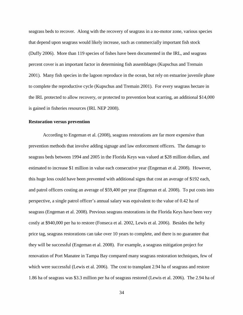
34
seagrass beds to recover. Along with the recovery of seagrass in a no-motor zone, various species
that depend upon seagrass would likely increase, such as commercially important fish stock
(Duffy 2006). More than 119 species of fishes have been documented in the IRL, and seagrass
percent cover is an important factor in determining fish assemblages (Kupschus and Tremain
2001). Many fish species in the lagoon reproduce in the ocean, but rely on estuarine juvenile phase
to complete the reproductive cycle (Kupschus and Tremain 2001). For every seagrass hectare in
the IRL protected to allow recovery, or protected to prevention boat scarring, an additional $14,000
is gained in fisheries resources (IRL NEP 2008).
Restoration versus prevention
According to Engeman et al. (2008), seagrass restorations are far more expensive than
prevention methods that involve adding signage and law enforcement officers. The damage to
seagrass beds between 1994 and 2005 in the Florida Keys was valued at $28 million dollars, and
estimated to increase $1 million in value each consecutive year (Engeman et al. 2008). However,
this huge loss could have been prevented with additional signs that cost an average of $192 each,
and patrol officers costing an average of $59,400 per year (Engeman et al. 2008). To put costs into
perspective, a single patrol officer’s annual salary was equivalent to the value of 0.42 ha of
seagrass (Engeman et al. 2008). Previous seagrass restorations in the Florida Keys have been very
costly at $940,000 per ha to restore (Fonseca et al. 2002, Lewis et al. 2006). Besides the hefty
price tag, seagrass restorations can take over 10 years to complete, and there is no guarantee that
they will be successful (Engeman et al. 2008). For example, a seagrass mitigation project for
renovation of Port Manatee in Tampa Bay compared many seagrass restoration techniques, few of
which were successful (Lewis et al. 2006). The cost to transplant 2.94 ha of seagrass and restore
1.86 ha of seagrass was $3.3 million per ha of seagrass restored (Lewis et al. 2006). The 2.94 ha of

35
seagrass was mitigated as transplants to enhance areas of degraded seagrass from boat traffic
(Lewis et al. 2006). The restoration methods of hand-transplanting individual shoots, hand-
planting shoot bundles, hand-planting bundles in peat pots, mechanized transplanting, modified
manual shovel planting, and prevention methods of creating a no motor zone combined were
successful in establishing and preserving 1.86 ha of seagrass (Lewis et al. 2006). The least costly
and most successful method used to restore seagrass beds was to create a no motor zone in which
0.77 ha of seagrass recolonized propeller scarred areas in 18 months (Lewis et al. 2006).
Future of seagrass in Mosquito Lagoon
Seagrass ecosystems are critical in creating habitat in areas of barren sediment, enhancing
community diversity, establishing intricate food webs, and stabilizing coastal sediments (Beck et
al. 2001, Burfeind and Stunz 2006, Duffy 2006). Seagrass beds in the Indian River Lagoon
provide a critical habitat for over 2000 species of invertebrates, fishes, birds and mammals, and are
a key reason why the IRL is the most productive and species-rich estuaries in North America
(IRL NEP 2008, Smithsonian Institution 2007). In my study, I looked at a major threat to seagrass
ecosystems, boat propeller scarring. I documented for the first time the severity of boat propeller
scarring in the IRL. In my manipulative experiments, I found that natural recovery was faster than
any restoration attempted method. Natural recovery of propeller scars can be as quick as 3 months
if some of the root structure and blades remain intact. Though my restoration methods were not
effective for scars in Mosquito Lagoon, the scars were naturally recolonized. Erosion was a
problem in both experiments, but despite bioturbation from rays and additional boat scarring, 40%
of all experimental scars returned to greater than 50% H. wrightii cover after 1 year. I agree with
Engeman et al. (2008) that more resources should focus on the prevention of scarring seagrass beds
than which restoration methods would work best, especially for Mosquito Lagoon where there are

36
thousands of hectares of healthy seagrass beds to recolonize scarred areas. Enhanced vigilance is
required from users, managers, and enforcers to protect the seagrass beds that are critical to the
biodiversity of Mosquito Lagoon and the IRL. Surely, prevention is the best way to preserve our
seagrass beds and the associated biodiversity for the future.

37
APPENDIX A:
LIST OF FIGURES
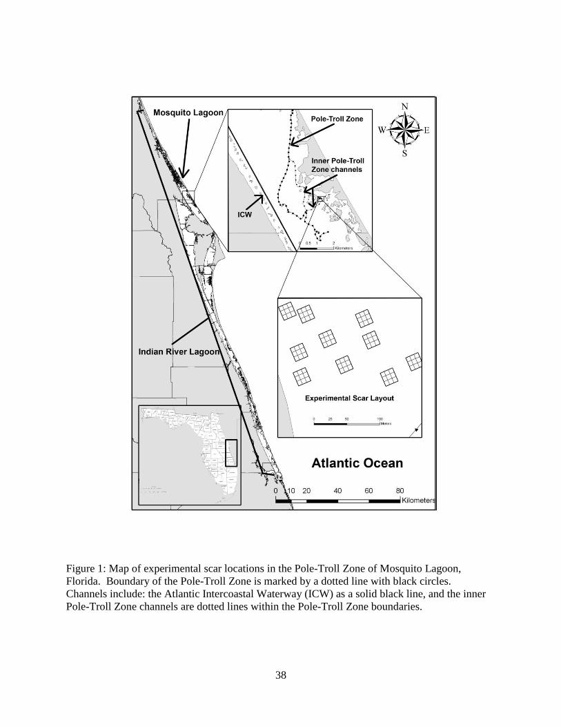
38
Figure 1: Map of experimental scar locations in the Pole-Troll Zone of Mosquito Lagoon,
Florida. Boundary of the Pole-Troll Zone is marked by a dotted line with black circles.
Channels include: the Atlantic Intercoastal Waterway (ICW) as a solid black line, and the inner
Pole-Troll Zone channels are dotted lines within the Pole-Troll Zone boundaries.

39
Figure 2: Halodule wrightii seagrass bed in Mosquito Lagoon, FL.

40
Figure 3: Location of 110 propeller scars measured in Mosquito Lagoon, FL. Scar type is color
coded to show the frequency of each scar type. From this view, the entire range of measured
scars is demonstrated, however not all scars can be seen due to overlap.

41
Function 1
86420-2-4
Fun
ctio
n 2
4
2
0
-2
-4
-6
4
3
2
1
Figure 4: Canonical Discriminant Analysis classification of 110 propeller scars in Mosquito
Lagoon. Scars were sorted into four groups. Type 1 scars are white circles, Type 2 scars are
black squares, Type 3 scars are black triangles, and Type 4 scars are white diamonds.
1
Scar dimensions
Se
ag
rass a
bu
nd
an
ce

42
Figure 5: Scar types identified from measuring 110 scars in Mosquito Lagoon. Above diagram
simplifies what was seen in each of the photographs below.
Figure 6: Frequency of scar types in Mosquito Lagoon (n = 110).
27.3%
6.4%
10.0%
56.4% 1
2
3
4

43
Scar Type 1 width (cm)
120100806040200
Scar
Typ
e 1
dept
h (c
m)
20
10
0
Figure 7: Regression of Type 1 scar width versus scar depth. Scar Type 1 was used to show the
best correlation (r2 = 0.476, p < 0.001), because other scar types (2-4) did not have depth.
Scar Type 1 width (cm)
Sca
r T
ype
1 d
ep
th (
cm
)

44
Scar Type
4321
mea
n %
fra
ctio
n (g
)
120
100
80
60
40
20
0
Figure 8: Mean percent of sediment grain size fractions and organic content per scar type.
Percent sediment fraction sizes are listed in order < 1mm is light grey cross hatch, 1 mm is dark
grey cross hatch, 2 mm is solid black, 5 mm is solid white, > 5mm is solid light grey, and percent
organic content is solid dark grey. Using a one-way ANOVA, only scar Type 1 and 4 were
significantly different in all fraction sizes, and size < 1mm showed the greatest difference.
Scar Type
Me
an
% f
ractio
n (
g)
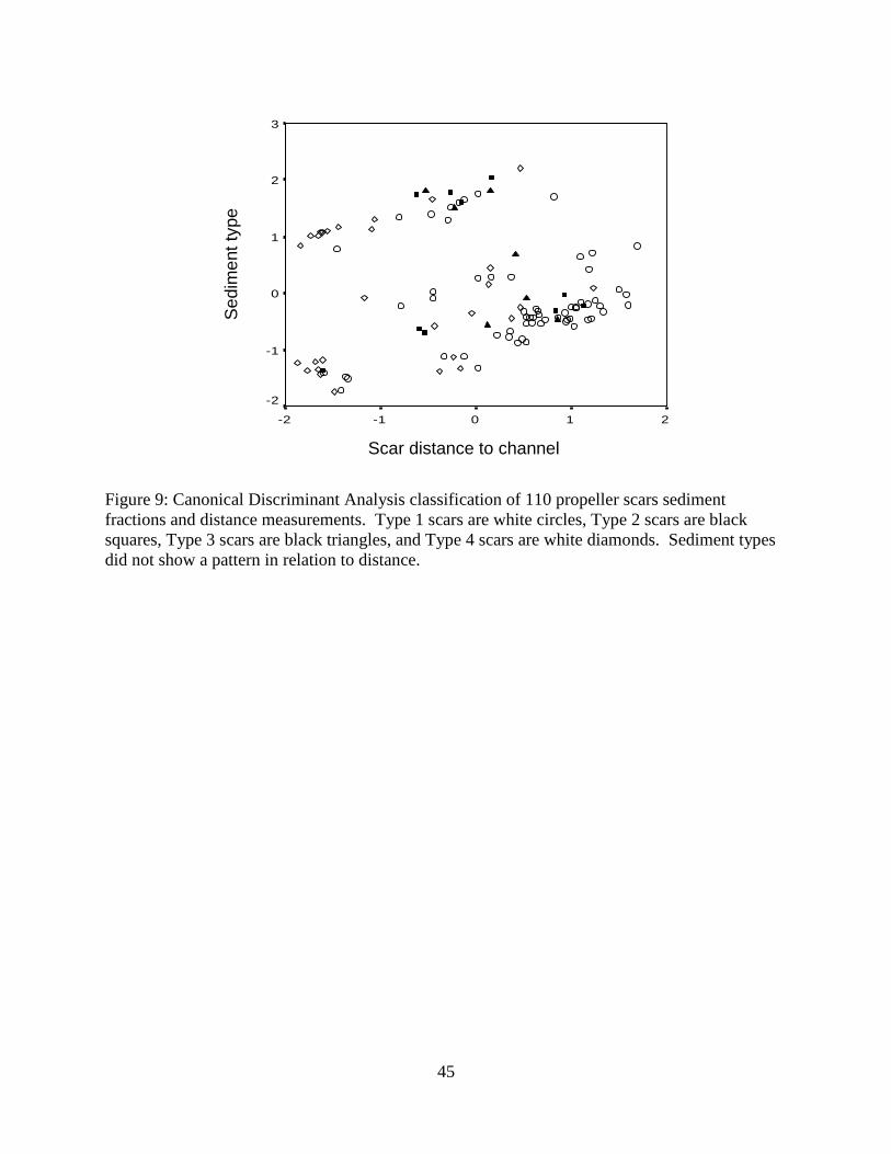
45
scar distance to channel
210-1-2
sedi
men
t typ
e
3
2
1
0
-1
-2
Figure 9: Canonical Discriminant Analysis classification of 110 propeller scars sediment
fractions and distance measurements. Type 1 scars are white circles, Type 2 scars are black
squares, Type 3 scars are black triangles, and Type 4 scars are white diamonds. Sediment types
did not show a pattern in relation to distance.
Scar distance to channel
Se
dim
ent
type

46
Figure 10: Layout of one block of experimental scars. Each block was 18 x18 m and was divided
into 9 squares, of which only 8 had a scar treatment. A square was 6 x 6 m containing a single
scar treatment in the center.
Figure 11: Setup of a one set of treatments in a large grid (block). An 18 x 18 m perimeter was
marked off with yellow rope, and a PVC pole was placed every 6 m. Scars were created in the
center of each 6 x 6 m square and marked with a short PVC pole at each end. All PVC grid
poles were marked with a GPS location and then removed. After the scars were created, only the
2 PVC scar markers remained to mark the ends of each scar.
6 m

47
Figure 12: PVC stake marking the end of an experimental scar.
Figure 13: PVC plow 32 cm in diameter. Device used to make experimental propeller scars the
same width, depth, and scar slope angle.
2.5 cm
32 cm
48
Figure 14: Arrow points to H. wrightii attached to garden staple with a twist tie in a scar filled
with sand. This is an eroded staple, making it is easier to see how H. wrightii was attached with
a red twist tie.
4 cm

49
A ug07 O ct07 D ec07 F eb08 A pr08 Jun08 A ug08
Te
mp
era
ture
(C
)
16
18
20
22
24
26
28
30
32
Figure 15: Mean water temperature on sampling dates (± S.E.) at location of manipulative
experiments (n = 3).
A ug07 O c t07 D ec07 F eb08 A p r08 Jun08 A ug08
Sa
linit
y (
pp
t)
32
34
36
38
40
42
44
46
Figure 16: Mean salinity (± S.E.) at location of manipulative experiments on sampling dates
(n = 3).

50
A ug-07 O c t-07 D ec-07 F eb -08 A p r-08 Jun -08 A ug -08
wa
ter
cla
rity
de
pth
(c
m)
30
35
40
45
50
55
60
Figure 17: Mean water clarity depth (± S.E.) at location of manipulative experiments on
sampling dates (n = 3). Maximum measurement possible using turbitdity tube was 60 cm.
A ug07 O c t07 D ec07 F eb08 A p r08 Jun08 A ug08
de
pth
(cm
)
30
40
50
60
70
80
90
a
a
a
a
a
aa
a
Figure 18: Mean water depth (± S.E.) of experimental scar locations of manipulative experiments
(n = 10). Measurements were analyzed with Kruskal-Wallis rank test with a Bonferroni
correction of p < 0.006. Treatments that were significantly different on a single day are shown
with different letters.

51
A ug07 O c t07 D ec07 F eb08 A p r08 Jun08 A ug08
Ha
lod
ule
sh
oo
ts
0
50
100
150
200
250
300
350
a
a
a
a
a
a
aa
Figure 19: Mean surrounding scar H. wrightii density (± S.E.) per 25 x 25 cm area in
experimental scar replicate blocks. Measurements were analyzed with Kruskal-Wallis rank test
with a Bonferroni correction of p < 0.006. Treatments that were significantly different on a
single day are shown with different letters.
A ug07 O c t07 D ec07 F eb08 A p r08 Jun08 A ug08
% H
alod
ule
cove
r
0
20
40
60
80
100
120
aa
a
a
a
a
a
a
Figure 20: Mean surrounding scar H. wrightii percent cover (± S.E.) per 25 x 25 cm area in
experimental scar replicate blocks. Measurements were analyzed with Kruskal-Wallis rank test
with a Bonferroni correction of p < 0.006. Treatments that were significantly different on a
single day are shown with different letters.

52
A ug07 O ct07 D ec07 F eb08 A pr08 Jun08 A ug08
can
op
y h
eig
ht
(cm
)
15
20
25
30
35
40
45
50
55
a
a
a
a
a
a
a
a
Figure 21: Mean surrounding scar H. wrightii canopy height (± S.E.) in experimental scar
replicate blocks. Measurements were analyzed with Kruskal-Wallis rank test with a Bonferroni
correction of p < 0.006. Treatments that were significantly different on a single day are shown
with different letters.

53
A ug07 O c t07 D ec07 F eb08 A p r08 Jun08 A ug08
Ha
lod
ule
sh
oo
ts
0
50
100
150
200
250
300
a
b
c
b
bb
aa
b
a
a
a
aa
b
b
aa
a
a
a a
b
a
aa
Figure 22: Natural recovery experimental scar H. wrightii shoot density per 25 x 25 cm area
(± S.E). Type 1 are black circles, Type 2 are white triangles, Type 3 are black squares, Type 4
are white diamonds, and control are black triangles. Measurements were analyzed with Kruskal-
Wallis rank test with a Bonferroni correction of p < 0.006. Treatments that were significantly
different on a single day are shown with different letters.

54
A ug07 O c t07 D ec07 F eb08 A p r08 Jun08 A ug08
% H
alo
du
le c
ov
er
0
20
40
60
80
100
aa
b
aa
b
c
b
b b
a
a
a
b
b
b
a
Figure 23: Natural recovery experimental scar H. wrightii percent cover per 25 x 25 cm area
(± S.E). Type 1 are black circles, Type 2 are white triangles, Type 3 are black squares, Type 4
are white diamonds, and control are black triangles. Measurements were analyzed with Kruskal-
Wallis rank test with a Bonferroni correction of p < 0.006. Treatments that were significantly
different on a single day are shown with different letters.

55
A ug07 O c t07 D ec07 F eb08 A p r08 Jun08 A ug08
can
op
y h
eig
ht
(cm
)
0
10
20
30
40
50
a
b
c
a
a
aa
a
b
b
b
b
cc c
d
a
b
a
b
d
c
Figure 24: Natural recovery experimental scar H. wrightii canopy height (± S.E). Type 1 are
black circles, Type 2 are white triangles, Type 3 are black squares, Type 4 are white diamonds,
and control are black triangles. Measurements were analyzed with Kruskal-Wallis rank test with
a Bonferroni correction of p < 0.006. Treatments that were significantly different on a single day
are shown with different letters.

56
A ug07 O c t07 D ec07 F eb08 A p r08 Jun08 A ug08
% r
oo
t c
ov
er
0
20
40
60
80
100
b
a
a
a
b
b
b
a
a
a
c
b
b
a
a
b
b
Figure 25: Natural recovery experimental scar percent root cover per 25 x 25 cm area (± S.E).
Type 1 are black circles, Type 2 are white triangles, Type 3 are black squares, and Type 4 are
white diamonds. Measurements were analyzed with Kruskal-Wallis rank test with a Bonferroni
correction of p < 0.006. Treatments that were significantly different on a single day are shown
with different letters.

57
A ug07 O c t07 D ec07 F eb08 A p r08 Jun08 A ug08
% le
af
litte
r c
ov
er
0
20
40
60
80
100
a
a
a
a
bb
b
b
aa
a
a
b
b
Figure 26: Natural recovery experimental scar percent leaf litter cover per 25 x 25 cm area
(± S.E). Type 1 are black circles, Type 2 are white triangles, Type 3 are black squares, and Type
4 are white diamonds. Measurements were analyzed with Kruskal-Wallis rank test with a
Bonferroni correction of p < 0.006. Treatments that were significantly different on a single day
are shown with different letters.

58
A ug07 O c t07 D ec07 F eb08 A p r08 Jun08 A ug08
sc
ar
de
pth
(c
m)
0
2
4
6
8
10
12
a
b
c cc
b
b
b
b
a
a
a
a
a
a
a
c c b b
Figure 27: Natural recovery experimental scar depth (± S.E). Type 1 are black circles, Type 2
are white triangles, Type 3 are black squares, and Type 4 are white diamonds. Measurements
were analyzed with Kruskal-Wallis rank test with a Bonferroni correction of p < 0.006.
Treatments that were significantly different on a single day are shown with different letters.

59
A ug07 O c t07 D ec07 F eb08 A p r08 Jun08 A ug08
sc
ar
wid
th (
cm
)
0
10
20
30
40
50
60
a
b
a
a
b bbb
a
a
a
a
a
Figure 28: Natural recovery experimental scar width (± S.E). Type 1 are black circles, Type 2
are white triangles, Type 3 are black squares, and Type 4 are white diamonds. Measurements
were analyzed with Kruskal-Wallis rank test with a Bonferroni correction of p < 0.006.
Treatments that were significantly different on a single day are shown with different letters.

60
A ug07 O c t07 D ec07 F eb08 A p r08 Jun08 A ug08
sc
ar
an
gle
in
de
gre
es
0
10
20
30
40
50
a
b
a
a
a
b
b
b b b
a
a
a
a
b
bc
Figure 29: Natural recovery experimental scar slope angle density (± S.E). Type 1 are black
circles, Type 2 are white triangles, Type 3 are black squares, and Type 4 are white diamonds.
Measurements were analyzed with Kruskal-Wallis rank test with a Bonferroni correction of
p < 0.006. Treatments that were significantly different on a single day are shown with different
letters.

61
> 5 m m 5 m m 2 m m 1 m m < 1m m
Pe
rce
nt
fra
cti
on
0
10
20
30
40
50
60
In itia l
F ina l: T ype 1
F ina l: T ype 2
F ina l: T ype 3
F ina l: T ype 4
F ina l: C on tro l
Figure 30: Natural recovery experiment mean percent sediment fractions (± S.E.) from before
scar creation and from within scars after 1 year (Kruskal-Wallis: p < 0.05). Bar sections are
labeled in order from left to right: initial, Type 1 (final), Type 2 (final), Type 3 (final), Type 4
(final), and control (final).

62
Initi
a l
Fin
a l: T
ype 1
Fin
a l: T
ype 2
Fin
a l: T
ype 3
Fin
a l: T
ype 4
Fin
a l: C
on tro l
Pe
rce
nt
org
an
ic
0
1
2
3
4
5
6
Figure 31: Natural recovery experiment mean percent organic content (± S.E) from before scar
creation and from within scars after 1 year (Kruskal-Wallis: p < 0.05).

63
A ug07 O c t07 D ec07 F eb08 A p r08 Jun08 A ug08
Ha
lod
ule
sh
oo
ts
0
50
100
150
200
250
300
a
b
a
a a
a
a
a
a
b b b
bb
b
b
Figure 32: Restoration experimental scar H. wrightii density shoot density per 25 x 25 cm
(± S.E). Controls are white triangles, Type 1 are black circles, plant-only are black squares, fill
only are white diamonds, and plant and fill are black triangles. Measurements were analyzed
with Kruskal-Wallis rank test with a Bonferroni correction of p < 0.006. Treatments that were
significantly different on a single day are shown with different letters.

64
A ug07 O c t07 D ec07 F eb08 A p r08 Jun08 A ug08
% H
alo
du
le c
ov
er
0
20
40
60
80
100
a
b
a
aa
a
a
aa
b b b
bb
b
b
Figure 33: Restoration experimental scar H. wrightii percent cover per 25 x 25 cm area (± S.E).
Control are white triangles, Type 1 are black circles, plant-only are black squares, fill only are
white diamonds, and plant and fill are black triangles. Measurements were analyzed with
Kruskal-Wallis rank test with a Bonferroni correction of p < 0.006. Treatments that were
significantly different on a single day are shown with different letters.

65
A ug07 O c t07 D ec07 F eb08 A p r08 Jun08 A ug08
ca
no
py
he
igh
t (c
m)
0
10
20
30
40
50
aa
a
aa
a
a
a
b b
b
b
b
b
b
Figure 34: Restoration experimental scar H. wrightii canopy height (± S.E). Control are white
triangles, Type 1 are black circles, plant-only are black squares, fill only are white diamonds, and
plant and fill are black triangles. Measurements were analyzed with Kruskal-Wallis rank test
with a Bonferroni correction of p < 0.006. Treatments that were significantly different on a
single day are shown with different letters.

66
A ug07 O c t07 D ec07 F eb08 A p r08 Jun08 A ug08
% r
oo
t c
ov
er
0
10
20
30
40
50
60
a a a
a a
a
a
a
Figure 35: Restoration experimental scar percent root cover per 25 x 25 cm area (± S.E). Type 1
are black circles, plant-only are white triangles, fill only are black squares, and plant and fill are
white diamonds. Measurements were analyzed with Kruskal-Wallis rank test with a Bonferroni
correction of p < 0.006. Treatments that were significantly different on a single day are shown
with different letters.

67
A ug07 O c t07 D ec07 F eb08 A p r08 Jun08 A ug08
% l
ea
f lit
ter
co
ve
r
0
20
40
60
80
100
a
a
a
a
a
a
a
Figure 36: Restoration experimental scar percent leaf litter cover per 25 x 25 cm area (± S.E).
Type 1 are black circles, plant-only are white triangles, fill only are black squares, and plant and
fill are white diamonds. Measurements were analyzed with Kruskal-Wallis rank test with a
Bonferroni correction of p < 0.006. Treatments that were significantly different on a single day
are shown with different letters.

68
A ug07 O c t07 D ec07 F eb08 A p r08 Jun08 A ug08
sc
ar
de
pth
(c
m)
0
2
4
6
8
10
12
14
16
a
b
a
a
a
b
b b b b b b
a
a
a
a
Figure 37: Restoration experimental scar depth (± S.E). Control are white triangles, Type 1 are
black circles, plant-only are black squares, fill only are white diamonds, and plant and fill are
black triangles. Measurements were analyzed with Kruskal-Wallis rank test with a Bonferroni
correction of p < 0.006. Treatments that were significantly different on a single day are shown
with different letters.
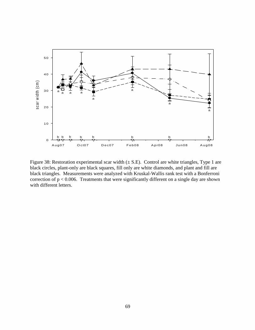
69
A ug07 O c t07 D ec07 F eb08 A p r08 Jun08 A ug08
sc
ar
wid
th (
cm
)
0
10
20
30
40
50
aa a a
a
a
a
a
b b b b b b b b
Figure 38: Restoration experimental scar width (± S.E). Control are white triangles, Type 1 are
black circles, plant-only are black squares, fill only are white diamonds, and plant and fill are
black triangles. Measurements were analyzed with Kruskal-Wallis rank test with a Bonferroni
correction of p < 0.006. Treatments that were significantly different on a single day are shown
with different letters.

70
A ug07 O c t07 D ec07 F eb08 A p r08 Jun08 A ug08
sc
ar
an
gle
in
de
gre
es
0
10
20
30
40
50
a
b
aa
a
b
b
a
a
a
a
b b b b b
Figure 39: Restoration experimental scar slope angle density (± S.E). Control are white
triangles, Type 1 are black circles, plant-only are black squares, fill only are white diamonds, and
plant and fill are black triangles. Measurements were analyzed with Kruskal-Wallis rank test
with a Bonferroni correction of p < 0.006. Treatments that were significantly different on a
single day are shown with different letters.

71
> 5m m 5 m m 2 m m 1 m m < 1m m
Pe
rce
nt
fra
cti
on
0
10
20
30
40
50
60
In itia l
F ina l: C on tro l
F ina l: T ype 1
F ina l: P lan t on ly
F ina l: F ill on ly
F ina l: P lan t & fill
Figure 40: Restoration experiment mean percent sediment fractions (± S.E.) from before scar
creation and from within scars after 1 year (Kruskal-Wallis: p < 0.05). Bar sections are labeled
in order from left to right: initial, control (final), Type 1 (final), plant only (final), fill only
(final), and plant and fill (final).

72
Initi
a l
Fin
a l: C
on tro l
Fin
a l: P
lan t o
n ly
Fin
a l: F
ill o
n ly
Fin
a l: P
lan t &
fill
Pe
rce
nt
org
an
ic
0
1
2
3
4
5
6
Figure 41: Restoration experiment mean percent organic content (± S.E) from before scar
creation and from within scars after 1 year (Kruskal-Wallis: p < 0.05).

73
Figure 42: Types of erosion observed in experimental scars: A) holes, B) washouts, and C) sand
patches. The black rectangle represents the original scar dimensions, brown is bare sediment,
dark brown represents depth, and the green represents seagrass.
Figure 43: Bioturbation caused by a stingray. Stingray created a hole and unburied a row of
Halodule wrightii transplants on staples, then left behind a pile of feces. In the left picture the
arrow points to a close-up of excrement pile in hole, and in right picture the arrow points to a
close up of the eroded staples next to the excrement pile.
4 cm 4 cm

74
Figure 44: Boater illegally using main engine motor in Pole-Troll Zone and running directly over
the experiment site.
Figure 45: A PVC pole marking an experimental scar that was hit by main engine boat motor in
less than 0.5 m of water.
2 cm

75
APPENDIX B:
LIST OF TABLES

75
Table 1: Studies documenting existing and experimental propeller scar damage and recovery of seagrasses. No information = “-”.
Species Location Experimental
Scar(s)/ model(s)
n Recovery
time (years)
Scar depth (cm)
Scar width (cm)
Scar length
(m)
Scar area (m2)
Water depth (m)
Salinity (ppt)
Current/tidal action
Dominant sediment type
Citation
Halodule wrightii
Tampa Bay, FL Yes 3 0.9 - 4.6 10 25 4 - - - - quartz-sand Durako et al. 1992
Tampa Bay, FL No 41 0.6 - 1.5 - - - 10 0.4 30 - 32 - - Bell et al. 1999
Tampa Bay, FL No 6 0.3 0 35 40 - - - - - Hall et al. 2006b
Florida Keys No 6 1 0 35 40 - - - - - Hall et al. 2006b
Laguna Madre, TX No - - 1 - 4 32 46 - 1 < 50
wind driven currents
- Martin et al. 2008
Mosquito Lagoon, FL Yes 10 2.1 9 32 2 0.64 0.56 33-44
tidal change = 10 cm
fine, < 1 mm Grablow 2008
Syringodium filiforme
Florida Keys model - 3 10 - 20 100 1 1 - - - - Fonseca et al. 2000
Florida Keys Yes 5 0.3 10 50 1.5 - 0.1 - 1.5 - - - Hammerstrom et al. 2007
Florida Keys Yes 5 1 20 50 1.5 - 0.1 - 1.5 - - - Hammerstrom et al. 2007
Florida Keys Yes 5 1 40 50 1.5 - 0.1 - 1.5 - - - Hammerstrom et al. 2007
Thalassia testudinum
Biscayne Bay, FL Yes 2 2 -5 20 30 1 - - -
rapid tidal currents
slit-clay Zieman 1976
Tampa Bay, FL Yes 3 3.6 - 6.4 7 25 4 - - - - quartz-sand Durako et al. 1992
Tampa Bay, FL Yes 12 7.6 - 25 5 - 0.5 - - sand Dawes et al. 1997
Tampa Bay, FL No 12 4.3 - - - - 0.5 - - sand Dawes et al. 1997
Florida Keys model - 17.5 10 - 20 100 1 1 - - - - Fonseca et al. 2000
Puerto Rico No 10 - 3 - 12 25 - 76 - - 0.5 - 1.6 -
tidal change = 15 cm
- Uhrin & Holmquist 2003
Puerto Rico No 2 60 - - - 1200 - - - - Fonseca et al. 2004
Florida Keys model - 10.5 > 20 100 - - - - -
carbonate -sand Fonseca et al. 2004
Florida Keys No 1 30 150 - - 15 - - - - Krisch et al. 2005
Tampa Bay, FL No 6 4 0 35 40 - - - - - Hall et al. 2006b
Florida Keys No 6 4 0 35 40 - - - - - Hall et al. 2006b
Florida Keys Yes 5 0.3 10 50 1.5 - 0.1 - 1.5 - - - Hammerstrom et al. 2007
Florida Keys Yes 5 3 20 50 1.5 - 0.1 - 1.5 - - - Hammerstrom et al. 2007
Florida Keys Yes 5 3 40 50 1.5 - 0.1 - 1.5 - - - Hammerstrom et al. 2007

76
Table 2: Canonical Discriminant Analysis results classifying 110 propeller scar measurements
into four groups. Table shows the percentage of scars correctly classified according to the most
important predictor variables: shoot density, scar depth, scar % root cover, and scar canopy
height.
Classification Results
scar severity
Predicted Group Membership
Total 1 2 3 4
Original Count 1 58 2 1 1 62
2 1 9 0 1 11
3 1 0 5 1 7
4 0 0 1 29 30
% 1 93.5 3.2 1.6 1.6 100.0
2 9.1 81.8 .0 9.1 100.0
3 14.3 .0 71.4 14.3 100.0
4 .0 .0 3.3 96.7 100.0
91.8% of original grouped cases correctly classified.
Table 3: Mean scar measurements (± S.E.) for each scar type from 110 scars.
Scar
Type
Scar Depth
(cm)
Scar Width
(cm)
Scar Canopy
Height (cm)
Surrounding Canopy
Height (cm)
Water
Depth (cm)
1 9 ± 1 36 ± 2 0 ± 0 30 ± 1 44 ± 2
2 1 ± 1 42 ± 6 0 ± 0 32 ± 2 50 ± 6
3 1 ± 1 25 ± 6 2 ± 2 28 ± 2 36 ± 5
4 1 ± 1 20 ± 1 12 ± 1 28 ± 2 44 ± 3
overall 5 ± 1 32 ± 2 4 ± 1 29 ± 1 44 ± 1

77
Table 4: Mean scar density measurements (± S.E.) per 25 x 25 cm area for each scar type from
110 scars.
Scar
Type
H. wrightii
Shoots In
Scar
H. wrightii
Shoots
Surrounding
Scar
% H. wrightii
Cover In Scar
% H. wrightii
Cover
Surrounding
Scar
% Root
Cover
In Scar
% Drift
Algae
In Scar
% Leaf
Litter
In Scar
1 0 ± 0 157 ± 9 0 ± 0 54 ± 4 0 ± 0 4 ± 2 55 ± 5
2 0 ± 0 133 ± 14 0 ± 0 38 ± 6 0 ± 0 1 ± 1 32 ± 12
3 4 ± 4 140 ± 32 1 ± 1 39 ± 14 56 ± 15 4 ± 4 47 ± 18
4 44 ± 6 180 ± 10 25 ± 4 62 ± 5 73 ± 7 1 ± 1 10 ± 4
Overall 12 ± 3 160 ± 7 7 ± 2 54 ± 3 24 ± 4 3 ± 1 40 ± 4
Table 5: Canonical Discriminant Analysis results from classifying sediment fractions of 110
scars. This table shows the percentage of scars correctly classified according to original
identifications. Sediment fractions were not a good predictor of scar types.
Classification Results
scar severity
Predicted Group Membership
Total 1 2 3 4
Original Count 1 55 0 0 7 62
2 7 0 0 4 11
3 7 0 0 0 7
4 11 0 0 19 30
% 1 88.7 .0 .0 11.3 100.0
2 63.6 .0 .0 36.4 100.0
3 100.0 .0 .0 .0 100.0
4 36.7 .0 .0 63.3 100.0
67.3% of original grouped cases correctly classified.

78
Table 6: Mean experimental scar measurements (± S.E.) for scar types 1-4 and control in natural
recovery experiment. Measurements were taken eight times from August 2007 through August
2008.
Initial 2 weeks 1 month 2 months
mean SE mean SE mean SE mean SE
Type 1 scars
H. wrightii density (shoots per 25 x 25 cm) 0 0 0 0 0 0 0 0
H. wrightii canopy height (cm) 0 0 0 0 1 1 0 0
H. wrightii % cover (per 25 x 25 cm) 0 0 0 0 0 0 0 0
H. wrightii % root cover (per 25 x 25 cm) 0 0 0 0 0 0 0 0
Scar width (cm) 32 0 34 2 32 1 41 5
Scar depth (cm) 9 0 10 1 11 1 12 1
Scar angle (degrees) 45 0 38 4 41 4 31 7
% leaf litter cover 25 13 90 6 95 5 90 8
% drift algae cover 4 3 0 0 0 0 0 0
Scar side H. wrightii density (shoots per 25 x 25 cm) 144 15 132 12 147 18 163 12
Scar side H. wrightii canopy height (cm) 46 3 47 1 41 1 30 2
Scar side H. wrightii % cover (per 25 x 25 cm) 55 6 52 5 59 7 63 4
Type 2 scars
H. wrightii density (shoots per 25 x 25 cm) 0 0 0 0 10 6 5 4
H. wrightii canopy height (cm) 0 0 0 0 9 5 4 3
H. wrightii % cover (per 25 x 25 cm) 0 0 0 0 2 2 1 1
H. wrightii % root cover (per 25 x 25 cm) 0 0 0 0 8 5 5 5
Scar width (cm) 32 0 34 3 46 8 46 9
Scar depth (cm) 0 0 4 1 5 2 7 1
Scar angle (degrees) 0 0 14 4 23 9 29 9
% leaf litter cover 24 11 64 13 56 15 80 9
% drift algae cover 1 1 0 0 0 0 0 0
Scar side H. wrightii density (shoots per 25 x 25 cm) 135 11 132 14 146 13 177 9
Scar side H. wrightii canopy height (cm) 46 1 49 2 41 2 36 2
Scar side H. wrightii % cover (per 25 x 25 cm) 51 5 52 6 59 5 69 3
Type 3 scars
H. wrightii density (shoots per 25 x 25 cm) 0 0 27 4 35 19 30 10
H. wrightii canopy height (cm) 0 0 14 4 14 4 14 3
H. wrightii % cover (per 25 x 25 cm) 0 0 6 1 11 7 8 4
H. wrightii % root cover (per 25 x 25 cm) 91 4 80 10 45 9 25 8
Scar width (cm) 32 0 39 4 36 4 36 6
Scar depth (cm) 0 0 0 0 0 0 5 2
Scar angle (degrees) 0 0 0 0 7 7 12 7
% leaf litter cover 27 12 57 12 58 15 61 12
% drift algae cover 0 0 0 0 0 0 0 0
Scar side H. wrightii density (shoots per 25 x 25 cm) 155 19 135 12 136 17 185 17
Scar side H. wrightii canopy height (cm) 44 2 47 2 42 2 35 2
Scar side H. wrightii % cover (per 25 x 25 cm) 61 8 55 5 53 8 72 7

79
Initial 2 weeks 1 month 2 months
mean SE mean SE mean SE mean SE
Type 4 scars
H. wrightii density (shoots per 25 x25 cm) 151 12 92 9 127 17 143 10
H. wrightii canopy height (cm) 12 0 24 1 31 1 26 1
H. wrightii % cover (per 25 x 25 cm) 61 6 37 5 49 7 58 4
H. wrightii % root cover (per 25 x 25 cm) 98 2 98 3 78 8 85 6
Scar width (cm) 32 0 33 1 31 1 3 3
Scar depth (cm) 0 0 0 0 0 0 0 0
Scar angle (degrees) 0 0 0 0 0 0 0 0
% leaf litter cover 23 10 37 13 28 13 0 0
% drift algae cover 1 1 3 2 0 0 0 0
Scar side H. wrightii density (shoots per 25 x25 cm) 151 12 130 8 151 16 147 24
Scar side H. wrightii canopy height (cm) 44 1 47 1 43 1 33 2
Scar side H. wrightii % cover (per 25 x 25 cm) 59 4 57 3 60 6 57 10
Control (dense seagrass)
H. wrightii density (shoots per 25 x 25 cm) 147 14 119 11 143 11 143 14
H. wrightii canopy height (cm) 44 2 46 2 42 2 35 2
H. wrightii % cover (per 25 x 25 cm) 59 6 58 7 57 4 56 6 6
3 months 6 months 9 months 12 months
mean SE mean SE mean SE mean SE
Type 1 scars
H. wrightii density (shoots per 25 x 25 cm) 17 4 6 3 62 10 116 21
H. wrightii canopy height (cm) 19 2 7 3 21 2 25 2
H. wrightii % cover (per 25 x 25 cm) 5 2 0 0 27 5 46 9
H. wrightii % root cover (per 25 x 25 cm) 8 8 0 0 31 6 54 11
Scar width (cm) 36 3 41 4 25 2 22 3
Scar depth (cm) 9 1 11 1 7 1 4 1
Scar angle (degrees) 23 2 16 2 12 2 13 3
% leaf litter cover 88 9 88 7 28 7 35 11
% drift algae cover 0 0 8 5 8 4 0 0
Scar side H. wrightii density (shoots per 25 x25 cm) 145 13 79 14 229 23 229 27
Scar side H. wrightii canopy height (cm) 37 2 18 1 28 1 37 2
Scar side H. wrightii % cover (per 25 x 25 cm) 59 5 28 6 80 6 85 8
Type 2 scars
H. wrightii density (shoots per 25 x 25 cm) 11 4 13 5 67 10 115 20
H. wrightii canopy height (cm) 10 3 12 3 22 2 26 3
H. wrightii % cover (per 25 x 25 cm) 2 1 2 1 27 5 47 9
H. wrightii % root cover (per 25 x 25 cm) 2 1 2 1 31 5 53 10
Scar width (cm) 37 7 51 12 31 4 18 3
Scar depth (cm) 7 1 7 1 4 1 2 1
Scar angle (degrees) 18 3 13 4 8 2 3 2
% leaf litter cover 66 13 77 12 28 7 28 12
% drift algae cover 0 0 0 0 3 2 0 0
Scar side H. wrightii density (shoots per 25 x25 cm) 129 15 90 13 193 21 223 25
Scar side H. wrightii canopy height (cm) 37 2 22 2 30 2 36 2
Scar side H. wrightii % cover (per 25 x 25 cm) 51 6 33 6 73 8 84 7

80
3 months 6 months 9 months 12 months
mean SE mean SE mean SE mean SE
Type 3 scars
H. wrightii density (shoots per 25 x 25 cm) 24 7 28 9 105 34 154 31
H. wrightii canopy height (cm) 20 1 13 4 24 3 31 2
H. wrightii % cover (per 25 x 25 cm) 9 3 7 2 37 12 58 12
H. wrightii % root cover (per 25 x 25 cm) 18 8 7 2 44 11 57 12
Scar width (cm) 35 3 32 9 26 6 20 7
Scar depth (cm) 5 1 5 2 4 1 2 1
Scar angle (degrees) 13 4 5 2 9 2 4 2
% leaf litter cover 70 12 60 13 23 10 25 12
% drift algae cover 0 0 0 0 4 2 0 0
Scar side H. wrightii density (shoots per 25 x 25 cm) 130 16 77 12 264 34 245 26
Scar side H. wrightii canopy height (cm) 38 2 23 1 31 1 37 2
Scar side H. wrightii % cover (per 25 x 25 cm) 50 6 25 6 84 7 88 8
Type 4 scars
H. wrightii density (shoots per 25 x25 cm) 133 14 73 11 263 29 244 21
H. wrightii canopy height (cm) 36 2 20 1 31 1 37 2
H. wrightii % cover (per 25 x 25 cm) 54 6 25 6 89 7 89 5
H. wrightii % root cover (per 25 x 25 cm) 76 7 25 6 92 5 96 3
Scar width (cm) 1 1 0 0 0 0 0 0
Scar depth (cm) 0 0 0 0 0 0 0 0
Scar angle (degrees) 0 0 0 0 0 0 0 0
% leaf litter cover 2 1 4 3 0 0 7 5
% drift algae cover 7 7 0 0 0 0 0 0
Scar side H. wrightii density (shoots per 25 x25 cm) 129 10 72 12 253 27 250 25
Scar side H. wrightii canopy height (cm) 39 2 22 1 34 2 38 2
Scar side H. wrightii % cover (per 25 x 25 cm) 53 3 25 6 86 7 90 5
Control (dense seagrass)
H. wrightii density (shoots per 25 x25 cm) 112 16 80 15 233 28 271 16
H. wrightii canopy height (cm) 36 2 20 2 29 2 38 2
H. wrightii % cover (per 25 x 25 cm) 58 12 38 7 81 7 97 2

81
Table 7: Kruskal-Wallis test for mean differences in measurements among scar types in natural
recovery experiment. Since tests were repeated eight times (once for each time period), the
significance level was corrected to p = 0.006 using the Bonferroni method.
Initial 2 weeks 1 month 2 months
df χ2 Sig. χ
2 Sig. χ
2 Sig. χ
2 Sig.
H. wrightii density 4 45.036 0.000 44.625 0.000 36.749 0.000 40.498 0.000
H. wrightii canopy height (cm) 4 48.503 0.000 44.806 0.000 36.460 0.000 39.237 0.000
H. wrightii % cover 4 45.083 0.000 45.137 0.000 36.838 0.000 40.657 0.000
H. wrightii % root cover 3 36.081 0.000 33.745 0.000 28.384 0.000 29.697 0.000
Scar width (cm) 3 49.000 0.000 25.141 0.000 28.983 0.000 34.778 0.000
Scar depth (cm) 3 49.000 0.000 41.937 0.000 35.660 0.000 33.625 0.000
Scar angle (degrees) 3 49.000 0.000 40.889 0.000 30.627 0.000 20.809 0.000
% leaf litter cover 3 0.079 0.994 9.514 0.023 10.891 0.012 26.631 0.000
% drift algae cover 3 2.334 0.506 6.154 0.104 0.000 1.000 0.000 1.000
Scar side H. wrightii density 4 2.708 0.608 0.660 0.956 0.361 0.986 4.766 0.312
Scar side H. wrightii canopy height (cm) 4 2.081 0.721 1.699 0.791 1.148 0.887 6.741 0.150
Scar side H. wrightii % cover 4 1.628 0.804 1.056 0.901 0.483 0.975 4.422 0.352
3 months 6 months 9 months 12 months
df χ2 Sig. χ
2 Sig. χ
2 Sig. χ
2 Sig.
H. wrightii density 4 33.799 0.000 28.723 0.000 29.172 0.000 24.523 0.000
H. wrightii canopy height (cm) 4 36.881 0.000 10.061 0.039 15.311 0.004 19.711 0.001
H. wrightii % cover 4 36.718 0.000 31.715 0.000 28.911 0.000 24.707 0.000
H. wrightii % root cover 3 23.692 0.000 21.120 0.000 18.628 0.000 11.397 0.010
Scar width (cm) 3 38.062 0.000 35.831 0.000 34.696 0.000 27.320 0.000
Scar depth (cm) 3 36.907 0.000 29.359 0.000 33.041 0.000 19.249 0.001
Scar angle (degrees) 3 33.152 0.000 31.336 0.000 31.326 0.000 21.598 0.000
% leaf litter cover 3 21.876 0.000 21.137 0.000 21.186 0.000 5.051 0.168
% drift algae cover 3 3.000 0.392 6.154 0.104 5.064 0.167 0.000 1.000
Scar side H. wrightii density 4 3.112 0.539 2.035 0.729 3.672 0.452 2.708 0.608
Scar side H. wrightii canopy height (cm) 4 1.588 0.811 10.075 0.039 3.854 0.426 0.567 0.967
Scar side H. wrightii % cover 4 2.111 0.715 2.717 0.606 3.333 0.504 3.860 0.425

82
Table 8: Mean experimental scar measurements (± S.E.) for three restoration treatments, and
Type 1 scar control in restoration experiment. Measurements were taken eight times from August
2007 through August 2008.
Initial 2 weeks 1 month 2 months
mean SE mean SE mean SE mean SE
In-Scar Measurements for plant-only method
Rooted H. wrightii density (shoots per 25 x 25 cm) 0 0 0 0 0 0 2 2
H. wrightii canopy height (cm) 0 0 0 0 0 0 6 4
H. wrightii % cover (per 25 x 25 cm) 0 0 0 0 0 0 1 1
H. wrightii % root cover (per 25 x 25 cm) 0 0 0 0 0 0 1 1
Scar width (cm) 32 0 34 1 33 1 32 1
Scar depth (cm) 9 0 10 1 10 1 11 1
Scar angle (degrees) 45 0 45 4 32 5 35 9
% leaf litter cover 26 11 85 10 100 0 90 8
% drift algae cover 2 2 0 0 0 0 0 0
Scar side H. wrightii density (shoots per 25 x 25 cm) 154 23 149 13 174 14 168 11
Scar side H. wrightii canopy height (cm) 44 1 47 1 42 1 35 2
Scar side H. wrightii % cover (per 25 x 25 cm) 56 6 59 5 68 5 67 5
In-Scar Measurements for fill only method
Rooted H. wrightii density (shoots per 25 x 25 cm) 0 0 0 0 1 1 6 3
H. wrightii canopy height (cm) 0 0 0 0 3 3 6 3
H. wrightii % cover (per 25 x 25 cm) 0 0 0 0 1 1 1 1
H. wrightii % root cover (per 25 x 25 cm) 0 0 0 0 0 0 6 5
Scar width (cm) 32 0 31 1 34 4 35 3
Scar depth (cm) 0 0 1 1 1 1 7 2
Scar angle (degrees) 0 0 8 6 12 9 21 9
% leaf litter cover 27 9 73 13 56 15 70 12
% drift algae cover 2 1 0 0 3 3 0 0
Scar side H. wrightii density (shoots per 25 x 25 cm) 140 18 138 10 161 13 150 21
Scar side H. wrightii canopy height (cm) 46 1 45 1 41 1 33 2
Scar side H. wrightii % cover (per 25 x 25 cm) 54 8 55 4 65 5 57 9
In-Scar Measurements for fill and plant
Rooted H. wrightii density (shoots per 25 x 25 cm) 0 0 0 0 0 0 0 0
H. wrightii canopy height (cm) 0 0 0 0 0 0 0 0
H. wrightii % cover (per 25 x 25 cm) 0 0 0 0 0 0 0 0
H. wrightii % root cover (per 25 x 25 cm) 0 0 0 0 0 0 0 0
Scar width (cm) 32 0 37 3 37 2 46 7
Scar depth (cm) 0 0 2 1 6 2 9 2
Scar angle (degrees) 0 0 4.5 2 9 5 26 7
% leaf litter cover 19 9 71 11 76 13 88 7
% drift algae cover 1 1 0 0 0 0 0 0
Scar side H. wrightii density (shoots per 25 x 25 cm) 160 17 136 12 153 12 160 27
Scar side H. wrightii canopy height (cm) 47 2 49 2 40 2 31 2
Scar side H. wrightii % cover (per 25 x 25 cm) 63 7 62 7 62 5 59 10

83
Initial 2 weeks 1 month 2 months
mean SE mean SE mean SE mean SE
In-Scar Measurements for Control, Type 1 scar
Rooted H. wrightii density (shoots per 25 x 25 cm) 0 0 0 0 0 0 0 0
H. wrightii canopy height (cm) 0 0 0 0 0 0 0 0
H. wrightii % cover (per 25 x 25 cm) 0 0 0 0 0 0 0 0
H. wrightii % root cover (per 25 x 25 cm) 0 0 0 0 0 0 0 0
Scar width (cm) 32 0 34 2 32 1 41 5
Scar depth (cm) 9 0 10 1 11 1 12 1
Scar angle (degrees) 45 0 38 4 41 4 31 7
% leaf litter cover 25 13 90 6 95 5 90 8
% drift algae cover 4 3 0 0 0 0 0 0
Scar side H. wrightii density (shoots per 25 x 25 cm) 229 27 132 12 147 18 163 12
Scar side H. wrightii canopy height (cm) 46 3 47 1 41 1 30 2
Scar side H. wrightii % cover (per 25 x 25 cm) 55 6 52 5 59 7 63 4
3 months 6 months 9 months 12 months
mean SE mean SE mean SE mean SE
In-Scar Measurements for plant-only method
Rooted H. wrightii density (shoots per 25 x 25 cm) 2 1 9 3 62 13 91 8
H. wrightii canopy height (cm) 8 3 9 3 21 2 27 2
H. wrightii % cover (per 25 x 25 cm) 0 0 1 1 25 6 35 3
H. wrightii % root cover (per 25 x 25 cm) 0 0 1 1 30 7 44 4
Scar width (cm) 29 3 35 3 27 3 25 3
Scar depth (cm) 12 3 9 1 6 1 4 1
Scar angle (degrees) 20 3 15 2 11 2 11 4
% leaf litter cover 95 5 90 9 19 6 47 10
% drift algae cover 0 0 0 0 14 10 0 0
Scar side H. wrightii density (shoots per 25 x 25 cm) 141 13 81 9 238 19 238 18
Scar side H. wrightii canopy height (cm) 39 3 22 1 28 2 37 1
Scar side H. wrightii % cover (per 25 x 25 cm) 57 5 28 5 88 5 91 5
In-Scar Measurements for fill only method
Rooted H. wrightii density (shoots per 25 x 25 cm) 8 3 8 4 59 16 109 19
H. wrightii canopy height (cm) 15 3 8 5 18 3 29 3
H. wrightii % cover (per 25 x 25 cm) 3 1 2 1 24 7 42 8
H. wrightii % root cover (per 25 x 25 cm) 3 1 2 1 28 8 50 8
Scar width (cm) 34 2 38 4 37 9 24 4
Scar depth (cm) 9 1 7 2 7 1 4 1
Scar angle (degrees) 17 3 12 4 8 2 9 3
% leaf litter cover 93 5 90 9 41 11 41 12
% drift algae cover 0 0 0 0 4 3 0 0
Scar side H. wrightii density (shoots per 25 x 25 cm) 150 10 58 9 229 32 210 23
Scar side H. wrightii canopy height (cm) 37 2 21 1 29 2 35 2
Scar side H. wrightii % cover (per 25 x 25 cm) 59 4 20 4 78 8 80 7

84
3 months 6 months 9 months 12 months
mean SE mean SE mean SE mean SE
In-Scar Measurements for fill and plant
Rooted H. wrightii density (shoots per 25 x 25 cm) 12 8 3 2 55 12 62 21
H. wrightii canopy height (cm) 8 4 3 2 20 3 19 4
H. wrightii % cover (per 25 x 25 cm) 3 2 1 1 22 6 23 8
H. wrightii % root cover (per 25 x 25 cm) 5 5 0 0 28 7 25 9
Scar width (cm) 33 3 43 8 43 9 40 13
Scar depth (cm) 7 2 10 1 8 1 8 2
Scar angle (degrees) 26 9 18 4 13 2 16 3
% leaf litter cover 77 8 95 5 56 11 70 14
% drift algae cover 0 0 1 1 3 3 0 0
Scar side H. wrightii density (shoots per 25 x 25 cm) 136 17 81 11 242 33 213 23
Scar side H. wrightii canopy height (cm) 34 3 22 1 29 2 39 1
Scar side H. wrightii % cover (per 25 x 25 cm) 55 6 29 5 79 8 82 7
In-Scar Measurements for Control (Type 1 scar)
Rooted H. wrightii density (shoots per 25 x 25 cm) 17 4 6 3 62 10 116 21
H. wrightii canopy height (cm) 19 2 7 3 21 2 25 2
H. wrightii % cover (per 25 x 25 cm) 5 2 0 0 27 5 46 9
H. wrightii % root cover (per 25 x 25 cm) 8 8 0 0 31 6 54 11
Scar width (cm) 36 3 41 4 25 2 22 3
Scar depth (cm) 9 1 11 1 7 1 4 1
Scar angle (degrees) 23 2 16 2 12 2 13 3
% leaf litter cover 88 9 88 7 28 7 35 11
% drift algae cover 0 0 8 5 8 4 0 0
Scar side H. wrightii density (shoots per 25 x 25 cm) 144 15 79 14 229 23 229 27
Scar side H. wrightii canopy height (cm) 37 2 6 3 28 1 37 2
Scar side H. wrightii % cover (per 25 x 25 cm) 59 5 28 6 80 6 85 8
Table 9: Survival of three restoration treatments for Type 1 scars between August 2007 and
August 2008.
Initial 2 weeks 1 month 2 months 3 months 6 months 9 months 12 months
Plant-only method
Mean (± S.E.) planting units per scar
16 ± 0 10 ± 2 1 ± 0 0 0 0 0 0
Fill only method
Scars retaining sand 10 10 9 7 6 4 4 4
Fill and plant method
mean (± S.E.) planting units per scar
16 ± 0 10 ± 2 5 ± 2 1 ± 0 0 0 0 0
Scars retaining sand 10 10 9 8 6 6 6 1

85
Table 10: Kruskal-Wallis test for mean differences in measurements among three restoration
treatments, the Type 1 scar control, and the seagrass control in restoration experiment. Since
tests were repeated eight times (once for each time period), the significance level was corrected
to p = 0.006 using the Bonferroni method.
Initial 2 weeks 1 month 2 months
df χ2 Sig. χ
2 Sig. χ
2 Sig. χ
2 Sig.
H. wrightii density (shoots per 25 x 25 cm) 4 48.205 0.000 48.205 0.000 35.937 0.000 37.769 0.000
H. wrightii canopy height (cm) 4 48.209 0.000 48.205 0.000 45.046 0.000 36.363 0.000
H. wrightii % cover (per 25 x 25 cm) 4 48.209 0.000 48.205 0.000 35.660 0.000 37.789 0.000
H. wrightii % root cover (per 25 x 25 cm) 3 0.000 1.000 0.000 1.000 8.531 0.036 6.128 0.106
Scar width (cm) 3 49.000 0.000 31.142 0.000 27.981 0.000 25.628 0.000
Scar depth (cm) 3 49.000 0.000 40.950 0.000 28.122 0.000 21.858 0.000
Scar angle 3 49.000 0.000 36.084 0.000 29.703 0.000 11.431 0.000
% leaf litter cover 3 0.545 0.909 2.270 0.518 8.899 0.031 2.109 0.550
% drift algae cover 3 0.712 0.870 0.000 1.000 3.000 0.392 0.000 1.000
Scar side H. wrightii density (shoots per 25 x 25 cm) 4 0.791 0.940 2.069 0.723 3.942 0.414 1.485 0.829
Scar side H. wrightii canopy height (cm) 4 2.791 0.593 3.577 0.466 5.518 0.238 5.510 0.239
Scar side H. wrightii % cover (per 25 x 25 cm) 4 0.875 0.928 1.587 0.811 4.009 0.405 1.122 0.891
3 months 6 months 9 months 12 months
df χ2 Sig. χ
2 Sig. χ
2 Sig. χ
2 Sig.
H. wrightii density (shoots per 25 x 25 cm) 4 29.970 0.000 25.392 0.000 22.318 0.000 25.583 0.000
H. wrightii canopy height (cm) 4 28.728 0.000 18.018 0.000 13.797 0.008 17.175 0.002
H. wrightii % cover (per 25 x 25 cm) 4 32.811 0.000 28.582 0.000 22.611 0.000 25.735 0.000
H. wrightii % root cover (per 25 x 25 cm) 3 13.557 0.004 2.637 0.451 0.124 0.989 5.647 0.130
Scar width (cm) 3 26.306 0.000 24.504 0.000 25.985 0.000 21.467 0.000
Scar depth (cm) 3 24.277 0.000 22.528 0.000 25.059 0.000 15.900 0.003
Scar angle 3 24.932 0.000 23.063 0.000 24.975 0.000 14.907 0.005
% leaf litter cover 3 6.163 0.104 2.194 0.533 6.535 0.088 3.889 0.274
% drift algae cover 3 0.000 1.000 2.393 0.495 2.600 0.457 0.000 1.000
Scar side H. wrightii density (shoots per 25 x25 cm) 4 3.532 0.473 3.082 0.544 0.293 0.990 5.192 0.268
Scar side H. wrightii canopy height (cm) 4 1.944 0.746 4.077 0.396 1.105 0.893 2.143 0.709
Scar side H. wrightii % cover (per 25 x 25 cm) 4 1.322 0.858 3.538 0.472 0.582 0.965 5.775 0.217

86
Table 11: Mean (± S.E.) number of scars having a type of erosion per time period in each
treatment.
Scar Erosion Types: Type 1 Type 2 Type 3 Type 4 Type 5 Type 6 Type 7 Type 8 Total
Mean number of scars with washouts per time period
1 ± 0 1 ± 0 1 ± 0 0 ± 0 0 ± 0 1 ± 0 2 ± 0 2 ± 1 8
Mean number of scars turned into sand patches per time period
0 ± 0 1 ± 0 0 ± 0 0 ± 0 0 ± 0 0 ± 0 0 ± 0 1 ± 0 2
Mean number of scars with holes per time period
1 ± 0 1 ± 0 1 ± 1 0 ± 0 0 ± 0 1 ± 0 3 ± 1 3 ± 1 11

87
LITERATURE CITED
Beck MW, Heck KL, Able KW, Childers DL, Eggleston DB, Gillanders B, Halpern BM, Hays
CG, Hoshino K, Minello TJ, Orth RJ, Sheridan PF, Weinstein MP (2001) The
identification, conservation, and management of estuarine and marine nurseries for fish
and invertebrates. BioScience 51:633-641
Bell SS, Robbins BD, Jensen SL (1999) Gap dynamics in a seagrass landscape. Ecosystems
2:493-504
Bostrom C, Jackson EL, Simenstad CA (2006) Seagrass landscapes and their effects on
associated fauna: a review. Estuarine, Coastal, and Shelf Science 68:383-403
Burfeind DD, Stunz GW (2006) The effects of boat propeller scarring intensity on nekton
abundance in subtropical seagrass meadows. Marine Biology 148:953-962
Campbell ML (2002) Getting the foundation right: a scientifically based management framework
to aid in the planning and implementation of seagrass transplant efforts. Bulletin of
Marine Science 71(3):1405-1414
Dawes CJ, Andorfer J, Rose C, Uranowski C, Ehringer N (1997) Regrowth of the seagrass
Thalassia testudinum into propeller scars. Aquatic Botany 59:139-155
Duarte CM (2002) The future of seagrass meadows. Environmental Conservation 29(2):192-206
Duarte CM, Cebrián J (1996) The fate of marine autotrophic production. Limnology and
Oceanography 41:1758–1766
Duffy JE (2006) Biodiversity and the functioning of seagrass ecosystems. Marine Ecology
Progress Series 311:233-250
Dunton KH (1996) Photosynthetic production and biomass of the subtropical seagrass Halodule
wrightii along an estuarine gradient. Estuaries 19(2B):436-447
Durako MJ, Hall MO, Sargent F, Peck S (1992) Propeller Scars in Seagrass Beds: An
Assessment and Experimental Study of Recolonization in Weedon Island State Preserve,
Florida. Proceedings of the Nineteenth Annual Conference on Wetland Restoration and
Creation. Hillsborough Community College, Plant City, FL
Dybas CL (2002) Florida’s Indian River Lagoon: an estuary in transition. BioScience 52(7):554-
599
Engeman RM, Duquesnel JA, Cowan EM, Smith HT, Shwiff SA, Karlin M (2008) Assessing
boat damage to seagrass bed habitat in a Florida park from a bioeconomic perspective.
Journal of Coastal Research 24(2):527-532
88
Erftemeijer PLA, Lewis RRR (2006) Environmental impacts of dredging on seagrasses: a
review. Marine Pollution Bulletin 52:1553-1572
Fabiano M, Danovaro R, Fraschetti S (1995) A three-year time series of elemental and
biochemical composition of organic matter in the subtidal sediments of the Ligurian Sea
(northwest Mediterranean). Continental Shelf Research 15:1453-1469
Fonseca MS, Whitfield PE, Kenworthy WJ, Colby DR, Julius BE (2004) Use of two spatially
explicit models to determine the effect of injury geometry on natural recovery. Aquatic
Conservation: Marine and Freshwater Ecosystems 14:281-298
Fonseca MS, Kenworthy WJ, Julius BE, Shutler S, Fluke S (2002) Seagrasses. In: Perrow MR,
Davy AJ (eds) Handbook of Ecological Restoration, Volume 2, Restoration in Practice.
Cambridge University Press, Cambridge, UK
Fonseca MS, Julius BE, Kenworthy WJ (2000) Integrating biology and economics in seagrass
restoration: How much is enough and why? Ecological Engineering 15:227-237
Fonseca MS, Kenworthy WJ, Thayer GW (1998) Guidelines for the conservation and restoration
of seagrasses in the United States and adjacent waters. In: NOAA Coastal Ocean Program
Decision Analysis Series No. 12. NOAA Coastal Office, Silver Spring, MD
FWC, Florida Fish and Wildlife Conservation Commission Legislative Proposal (2008)
Establishing penalties for seagrass damage. Divison of Law Enforcement, Tallahassee,
FL
Handley L, Altsman D, DeMay R, (2007) Seagrass status and trends in the Northern Gulf of
Mexico:1940-2002: U.S. Geological Survey Scientific Investigations Report 2006-5287
and U.S. Environmental Protection Agency 855-R-04-003
Hall CR, Provancha JA, Oddy DM, Lowers RL, Drese JD (2001) Canaveral National Seashore
water quality and aquatic resource inventory. NASA Technical Memorandum 2001-
210261, Kennedy Space Center, FL
Hall LM, Hanisak MD, Virnstein RV (2006a) Fragments of the seagrasses Halodule wrightii and
Halophila johnsonii as potential recruits in Indian River Lagoon, Florida. Marine
Ecology Progress Series 310:109-117
Hall MO, Merello M, Kenworthy WJ, Berns D, Ferenc K, Kunzelman J, Hall F, Hyniova J
(2006b) Developing techniques to enhance the recovery rates of propeller scars in
turtlegrass (Thalassia testudinum) meadows, Report F2319-02-F. U.S. Fish and Wildlife
Service
Hammerstrom KK, Kenworthy WJ, Whitfield PE, Merello MF (2007) Response and recovery
dynamics of seagrasses Thalassia testudinum and Syringodium filiforme and macroalgae
in experimental motor vessel disturbances. Marine Ecology Progress Series 345:83-92

89
Hemminga M, Duarte CM (2000) Seagrass Ecology. Cambridge, UK: Cambridge University
Press. Independent World Commission on the Oceans (1998) The Ocean. Our Future.
Cambridge, UK: Cambridge University Press
IRL NEP, Indian River Lagoon National Estuary Plan (2008) Indian River Lagoon assessment
and analysis update, final report, contract no. 24706. Indian River Lagoon National
Estuary Program Palm Bay, FL
Kirsch KD, Barry AB, Fonseca MS, Whitfield PE, Meehan SR, Kenworthy WJ, Julius BE
(2005) The mini-312 program – An expedited damage assessment and restoration process
for seagrasses in the Florida Keys National Marine Sanctuary. Journal of Coastal
Research 40:109-119
Koch EW, Schopmeyer SA, Kyhn-Hansen C, Madden CJ, Peters JS (2007) Tropical seagrass
species tolerance to hypersalinity stress. Aquatic Botany 86:14-24
Kupschus S, Tremain D (2001) Associations between fish assemblages and environmental
factors in nearshore habitats of a subtropical estuary. Journal of Fish Biology 58:1383-
1403
Lewis RR, Marshall MJ, Bloom SA, Hodgson AB, Flynn LL (2006) Evaluation of the success of
seagrass mitigation at Port Manatee, Tampa Bay, Florida. In: Treat SF, Lewis RR (eds)
Seagrass Restoration: success, failure, and the cost of both. Lewis Environmental Inc.,
Valrico, FL
Marbá N, Duarte CM (1998) Rhizome elongation and seagrass clonal growth. Marine Ecology
Progress Series 174: 269–280
Marbá N, Hemminga MA, Duarte CM (2006) Resource translocation within seagrass clones:
allometric scaling to plant size and productivity. Oecologia 150:362-372
Martin SR, Onuf CP, Dunton KH (2008) Assessment of propeller and off-road vehicle scarring
in seagrass beds and wind-tidal flats of the southwestern Gulf of Mexico. Botanica
Marina 51:79-91
MINWR CCP, Merritt Island Wildlife Refuge Comprehensive Conservation Plan (2008) Merritt
Island National Wildlife Refuge, Titusville, FL
Orth RJ, Harwell MC, Bailey EM, Bartholomew A, Jawad JT, Lombana AV, Moore KA, Rhode
JM, Woods HE (2000) A review of issues in seagrass seed dormancy and germination:
implications for conservation and restoration. Marine Ecology Progress Series 200:277-
288
Parker JG (1983) A comparison of methods used for the measurement of organic matter in
marine sediments. Chemistry and Ecology 1:201-210

90
Sargent FJ, Leary TJ, Crewz DW, Kruer CR (1995) Scarring of Florida’s seagrasses: assessment
and management options. FMRI Technical Report TR-1. Florida Marine Research
Institute, St. Petersburg, Florida
Sheridan P, McMahan G, Hammerstrom K, Pulich W (1998) Factors affecting restoration of
Halodule wrightii to Galveston Bay, Texas. Restoration Ecology 6(2):144-158
Scheidt DM, Garreau CM (2007) Identification of watercraft use patterns in Canaveral National
Seashore. Final Report: Canaveral National Seashore PIMS Project no. 1021131
Smithsonian Institution (2007) Indian River Lagoon species inventory. Smithsonian Marine
Station at Fort Pierce, FL. Accessed 1 May. http://www.sms.si.edu/irlspec/index.htm
Smith NP (1993) Tidal and non-tidal flushing of Florida’s Indian River Lagoon. Estuaries
16(4):739-746
Steward JS, Virnstein RV, Lasi MA, Morris LJ, Miller JD, Hall LM, Tweedale WA (2006) The
impacts of the 2004 hurricanes on hydrology, water quality, and seagrass in the central
Indian River Lagoon, Florida. Estuaries and Coasts 29(6A):954-956
Terrados J, Duarte CM (1999) Experimental evidence of reduced particle resuspension within a
seagrass (Posidonia oceanica L.) meadow. Journal of Experimental Marine Biology and
Ecology 243:45–53
Thorhaug A (1986) Review of seagrass restoration efforts. Ambio 15(2):110-117
Uhrin AV, Holmquist JG (2003) Effects of propeller scarring on macrofaunal use of the seagrass
Thalassia testudinum. Marine Ecology Progress Series 250:61-70
Virnstein RW, Steward JS, Morris LJ (2007) Seagrass coverage trends in the Indian River
Lagoon System. Florida Scientist 70:397-404
Welsh DT (2000) Nitrogen fixation in seagrass meadows: regulation, plant-bacteria interactions
and significance to primary productivity. Ecology Letters 3:58-71
Zieman JC (1976) The ecological effects of physical damage from motor boats on turtle grass
beds in southern Florida. Aquatic Botany 2:127-139
![Halodule pinifolia]](https://static.fdocuments.net/doc/165x107/54e4cd8b4a7959c3668b51a2/halodule-pinifolia.jpg)


