HAL Id: hal-01669518https://hal.archives-ouvertes.fr/hal-01669518

Submitted on 16 Oct 2020

HAL is a multi-disciplinary open accessarchive for the deposit and dissemination of sci-entific research documents, whether they are pub-lished or not. The documents may come fromteaching and research institutions in France orabroad, or from public or private research centers.

L’archive ouverte pluridisciplinaire HAL, estdestinée au dépôt et à la diffusion de documentsscientifiques de niveau recherche, publiés ou non,émanant des établissements d’enseignement et derecherche français ou étrangers, des laboratoirespublics ou privés.

Recovering galaxy cluster gas density profiles withXMM-Newton and Chandra

I. Bartalucci, M. Arnaud, G.W. Pratt, A. Vikhlinin, E. Pointecouteau, W.R.Forman, C. Jones, P. Mazzotta, F. Andrade-Santos

To cite this version:I. Bartalucci, M. Arnaud, G.W. Pratt, A. Vikhlinin, E. Pointecouteau, et al.. Recovering galaxycluster gas density profiles with XMM-Newton and Chandra. Astronomy and Astrophysics - A&A,EDP Sciences, 2017, 608, pp.A88. 10.1051/0004-6361/201731689. hal-01669518

A&A 608, A88 (2017)DOI: 10.1051/0004-6361/201731689c© ESO 2017

Astronomy&Astrophysics

Recovering galaxy cluster gas density profileswith XMM-Newton and Chandra

I. Bartalucci1, 2, M. Arnaud1, 2, G. W. Pratt1, 2, A. Vikhlinin3, E. Pointecouteau4, W. R. Forman3, C. Jones3,P. Mazzotta3, 5, and F. Andrade-Santos3

1 IRFU, CEA, Université Paris-Saclay, 91191 Gif-Sur-Yvette, Francee-mail: iacopo.bartalucci@cea.fr

2 Université Paris Diderot, AIM, Sorbonne Paris Cité, CEA, CNRS, 91191 Gif-sur-Yvette, France3 Harvard-Smithsonian Center for Astrophysics, 60 Garden Street, Cambridge, MA 02138, USA4 IRAP, Université de Toulouse, CNRS, UPS, CNES, 31042 Toulouse, France5 Dipartimento di Fisica, Université di Roma Tor Vergata, via della Ricerca Scientifica 1, 00133 Roma, Italy

Received 1 August 2017 / Accepted 14 September 2017

ABSTRACT

We examined the reconstruction of galaxy cluster radial density profiles obtained from Chandra and XMM-Newton X-ray observa-tions, using high quality data for a sample of twelve objects covering a range of morphologies and redshifts. By comparing the resultsobtained from the two observatories and by varying key aspects of the analysis procedure, we examined the impact of instrumentaleffects and of differences in the methodology used in the recovery of the density profiles. We find that the final density profile shape isparticularly robust. We adapted the photon weighting vignetting correction method developed for XMM-Newton for use with Chandradata, and confirm that the resulting Chandra profiles are consistent with those corrected a posteriori for vignetting effects. Profiles ob-tained from direct deprojection and those derived using parametric models are consistent at the 1% level. At radii larger than ∼6′′, theagreement between Chandra and XMM-Newton is better than 1%, confirming an excellent understanding of the XMM-Newton PSF.Furthermore, we find no significant energy dependence. The impact of the well-known offset between Chandra and XMM-Newtongas temperature determinations on the density profiles is found to be negligible. However, we find an overall normalisation offset indensity profiles of the order of ∼2.5%, which is linked to absolute flux cross-calibration issues. As a final result, the weighted ratiosof Chandra to XMM-Newton gas masses computed at R2500 and R500 are r = 1.03 ± 0.01 and r = 1.03 ± 0.03, respectively. Ourstudy confirms that the radial density profiles are robustly recovered, and that any differences between Chandra and XMM-Newtoncan be constrained to the ∼2.5% level, regardless of the exact data analysis details. These encouraging results open the way for thetrue combination of X-ray observations of galaxy clusters, fully leveraging the high resolution of Chandra and the high throughput ofXMM-Newton.

Key words. methods: data analysis – galaxies: clusters: intracluster medium – X-rays: galaxies: clusters

1. Introduction

Clusters of galaxies provide valuable information on cosmology,from the physics driving galaxy and structure formation to thenature of dark energy (see e.g. Voit 2005; Allen et al. 2011).Clusters are primarily composed of dark matter, the baryoniccomponent being contained mainly in the form of hot ionisedplasma that fills the intra-cluster volume, namely the intra-cluster medium (ICM). The ICM emits in the X-ray band primar-ily via thermal Bremsstrahlung, which depends on the plasmadensity and temperature.

X-ray observations play a key role in studying the ICMemission. In particular, the advent of high resolution spectro-imaging observations from Chandra and XMM-Newton hasyielded a rich ensemble of observations to be studied and un-derstood. In the context of galaxy cluster observations these twosatellites are complementary: the unprecedented angular reso-lution of Chandra is well-suited to exploring the bright cen-tral parts, while the large effective area of XMM-Newton al-lows detection of the emission up to large radial distances,where the X-ray signal becomes very faint. A combination ofthese instruments can in principle be used to obtain more pre-cise (especially in the centre) and spatially extended profiles

(e.g. Bartalucci et al. 2017). However, previous works combin-ing datasets from the two satellites have found systematic differ-ences due to cross-calibration issues (e.g. Snowden et al. 2008;Mahdavi et al. 2013; Martino et al. 2014; Schellenberger et al.2015). For the hottest clusters, Chandra temperatures are foundto be higher than those of XMM-Newton by 10−15% whilethe flux offset is smaller, at ∼1−3%, and consistent with zero.Furthermore, as instruments are routinely monitored throughoutthe spacecraft lifetime and as in-flight calibration is undertaken,these systematic differences can evolve considerably dependingon the version of the calibration database, CALDB, used for eachsatellite.

Here we focus uniquely on the reconstruction of gas densityprofiles and the calculation of integrated gas masses fromXMM-Newton and Chandra data. The gas density should, inprinciple, be trivial to recover since the observed X-ray surfacebrightness is proportional to the line-of-sight integral of thesquare of the density, times the X-ray cooling function, whichin turn is almost independent of temperature in the soft energyband. Thus the absolute temperature calibration will have aminimal effect on the recovered density (shown explicitly inSect. 4.4). However, a number of other potential sources of

Article published by EDP Sciences A88, page 1 of 15

A&A 608, A88 (2017)

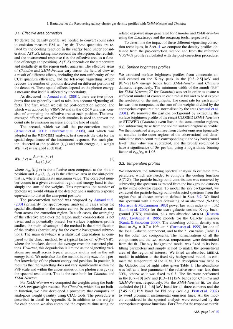
Table 1. Observational properties of the 12 clusters used in this work.

Cluster name RA Dec z NHa Chandra XMM-Newton Chandra XMM-Newton

exp. exp. (MOS1,2; PN) obs. ID obs. ID[J2000] [J2000] [1020 cm−3] [ ks] [ ks]

A1651 12 59 22.15 −04 11 48.24 0.084 1.81 10 7; 5 4185 0203020101A1650 12 58 41.48 −01 45 40.45 0.084 0.72 37 34; 30 7242 0093200101A1413 11 55 17.97 +23 24 21.99 0.143 1.84∗ 75 63; 52 5003 0502690201A2204 16 32 46.94 +05 34 32.63 0.152 6.97∗ 77 14; 10 7940 0306490201A2163 16 15 46.06 −06 08 52.36 0.203 16.50∗ 71 92; 65† 1653 0694500101A2390 21 53 36.82 +17 41 43.30 0.231 8.66 95 10; 8 4193• 0111270101MACS J1423.8+2404 14 23 47.92 +24 04 42.96 0.545 2.20 115 34; 22† 4195• 0720700301MACS J0717.5+3745b 07 17 31.75 +37 45 31.02 0.546 6.64 58 59; 52 16305 0672420201MACS J0744.9+3927 07 44 52.78 +39 27 26.63 0.698 5.66 50 52; 42† 6111 0551851201SPT-CL J2146−4633 21 46 34.72 −46 32 50.86 0.933 1.64 80 90; 64† 13469 0744400501SPT-CL J2341−5119 23 41 12.23 −51 19 43.05 1.003 1.21 50 64; 34† 11799 0744400401SPT-CL J0546−5345 05 46 37.22 −53 45 34.43 1.066 6.77 27 45; 33† 9336 0744400201

Notes. The coordinates indicate the position of the X-ray peak used as the centre for profile extraction. The peak was determined using Chandraobservations in the [0.7−2.5] keV band. (a) The neutral hydrogen column density was derived from the LAB survey (Kalberla et al. 2005). (b) TheX-ray peak is centred on the main structure, identified as region “B” in Limousin et al. (2016). (∗) The absorption value was estimated in a regionwhich maximises the S/N . (†) MOS 2 effective exposure times are 3−4% higher than MOS1, except for MACS J1423.8+2404, for which theMOS2 exposure time is 43 ks. (•) ACIS-S observations.

systematic difference still remain, including: the absolute fluxcalibration; the exclusion of substructure and point sources;for XMM-Newton, the correction for the point spread function(PSF); the method used to correct for the vignetting of theX-ray telescopes; or whether the analysis uses a parametric ora non-parametric approach. Here we have compared the ICMdensity profiles obtained using variations on two approachesdeveloped for statistical studies of clusters – that of the ChandraCluster Cosmology Project (CCCP; Vikhlinin et al. 2009a) forChandra, and that of REXCESS (Croston et al. 2008; Pratt et al.2009) for XMM-Newton. The Planck Collaboration have alsoused the latter method (e.g. Planck Collaboration XI 2011;Planck Collaboration Int. III 2013; Planck Collaboration XX2014). Our choice is motivated by the fact that each approach isrepresentative of a standard analysis for its respective satellite,while being sufficiently different in procedure (notably in thetreatment of vignetting, or in the choice of parametric vs.non-parametric modelling of the X-ray surface brightness) toallow investigation of some of the issues mentioned above.We can also use the exceptional PSF of Chandra to test therobustness of the XMM-Newton PSF correction procedure,which is one of the main analysis issues when reconstructing thecentral regions of the gas density profiles. This is particularlytrue for evolution studies, because of the decrease of the angularsize with the redshift. Hence we focus on a sample in a wideredshift range, up to z ∼ 1.

The paper is organised as follows: in Sect. 2 we present thesample of the clusters used in this work, and in Sect. 3 we de-tail the various data analysis steps and methods used to recon-struct the radial density distribution from the surface brightnessprofiles. In Sect. 4, we describe the tests we use to asses andquantify the robustness of the density profile reconstruction, anddetail the comparison between the two instruments. Our conclu-sions are presented in Sect. 6.

We adopted a cold dark matter cosmology with ΩM = 0.3,ΩΛ = 0.7 and H0 = 70 km Mpc−1 s−1 throughout. All errors arereported at the 1σ level. The quantity R500 is defined as the radiusat which the total density of the cluster is 500 times the criticaldensity.

2. Cluster sample

As this work is dedicated to a systematic comparison of the ICMproperties derived from Chandra and XMM-Newton observa-tions, we required (1) sufficient exposure time to allow extrac-tion of well-sampled radial profiles at least up to ∼R500; (2) awide redshift range to test the effect of different angular sizes onthe PSF reconstruction; (3) different X-ray morphologies to ex-amine the effect of features such as, for example, peaked or flatcentral emission. Following these criteria we defined a sampleof twelve clusters whose main observational properties are re-ported in Table 1. We limited our datasets to single observationsto simplify the analysis and avoid complications related to thecreation of mosaics.

All the clusters in our sample have been observed usingthe Chandra Advanced CCD Imaging Spectrometer (ACIS,Garmire et al. 2003) and the XMM-Newton European PhotonImaging Camera (EPIC). Chandra operates using a combina-tion of two charged coupled device (CCD) arrays, the ACIS-Imaging or the ACIS-Spectroscopy (ACIS-I and ACIS-S, re-spectively), where the focus can be placed on either. TheXMM-Newton EPIC instrument is composed of three cam-eras, MOS1, 2 (Turner et al. 2001) and PN (Strüder et al. 2001),which operate simultaneously. Chandra observations of A2390and MACSJ1423.8+2404 are ACIS-S, all the others are ACIS-I.

The Chandra observations of the six nearest clusters inTable 1 have previously been analysed in Vikhlinin et al. (2006,2009a, hereafter V06 and V09) using the CCCP procedure.The corresponding XMM-Newton observations were analysedin Planck Collaboration XI (2011) using the REXCESS analy-sis procedures. These published results are directly compared inSect. 4.1.

3. Data analysis

Appendix A summarises the basic data reduction, including pro-duction of calibrated event files, point source masking and back-ground estimation.

A88, page 2 of 15

I. Bartalucci et al.: Recovering galaxy cluster gas density profiles with XMM-Newton and Chandra

3.1. Effective area correction

To derive the density profile, we needed to convert count ratesto emission measure EM =

∫n2

e dv. These quantities are re-lated by the cooling function in the energy band under consid-eration, Λ(T,Z), taking into account the absorption, the redshift,and the instrumental response (i.e. the effective area as a func-tion of energy and position). Λ(T,Z) depends on the temperatureand metallicity in the region under analysis. The effective areasof Chandra and XMM-Newton vary across the field of view asa result of different effects, including the non-uniformity of theCCD quantum efficiency, and the telescope vignetting (whichreduces the number of photons detected on different portions ofthe detector). These spatial effects depend on the photon energy,a measure that itself is affected by uncertainty.

As discussed in Arnaud et al. (2001), there are two proce-dures that are generally used to take into account vignetting ef-fects. The first, which we call the post-correction method, andwhich was adopted by V06/V09 and in the CCCP analysis, con-sists of computing the effective area at each position. The area-averaged effective area for each annulus is used to convert thecount rate to emission measure along the line of sight.

The second, which we call the pre-correction method(Arnaud et al. 2001; Churazov et al. 2008), and which wasadopted in the REXCESS analysis, first corrects the data for thespatial dependence of the instrument response. For each pho-ton, detected at the position (i, j) and with energy e, a weightW(i, j, e) is assigned such that:

W(i, j, e) =Aeff (i0, j0, e)Aeff (i, j, e)

, (1)

where Aeff (i, j, e) is the effective area computed at the photonposition and Aeff (i0, j0, e) is the effective area at the aim-point,that is, where it attains its maximum value. The corrected num-ber counts in a given extraction region and energy band is thensimply the sum of the weights. This represents the number ofphotons we would obtain if the detector had a uniform responseequivalent to that at the aim-point position.

The pre-correction method was proposed by Arnaud et al.(2001) primarily for spectroscopic analysis in cases when thespatial distribution of the source cannot be considered as uni-form across the extraction region. In such cases, the averagingof the effective area over the region under consideration is nottrivial and is potentially biased. For surface brightness profilestudies, the main advantage of the method is the simplificationof the analysis (particularly for the cosmic background subtrac-tion). The main drawback is a statistical degradation as com-pared to the direct method, by a typical factor of

√〈W2〉/〈W〉,

where the brackets denote the average over the extracted pho-tons. However, this degradation is limited as the vignetting vari-ations are small across typical annulus widths and in the softenergy band. We note also that the method is only exact for a per-fect knowledge of the photon energy and position. In practice, itrequires that the vignetting does not vary significantly within thePSF scale and within the uncertainties on the photon energy (i.e.the spectral resolution). This is the case both for Chandra andXMM-Newton.

For XMM-Newton we computed the weights using the built-in SAS evigweight routine. For Chandra, which has no built-in function, we have developed a procedure that computes ananalogous weight quantity using CIAO tools. The procedure isdescribed in detail in Appendix B. In addition to the weight,for each photon we also computed the exposure time using the

related exposure maps generated for Chandra and XMM-Newtonusing the fluximage and the eexpmap tools, respectively.

To determine the impact of these different vignetting correc-tion techniques, in Sect. 4 we compare the density profiles ob-tained from the pre-correction method and from the referenceV06/V09 profiles calculated with the post-correction procedure.

3.2. Surface brightness profiles

We extracted surface brightness profiles from concentric an-nuli centred on the X-ray peak in the [0.3−2.5] keV and[0.7−2] keV energy bands from XMM-Newton and Chandradatasets, respectively. The minimum width of the annuli (3.3′′for XMM-Newton; 2′′ for Chandra) was set in order to ensure asufficient number of counts in each radial bin and to best exploitthe resolution of the instruments. The count rate for each annu-lus was then computed as the sum of the weights divided by theappropriate exposure time, normalised by the area (Arnaud et al.2001). We removed the particle background by extracting thesurface brightness profile of the recast CLOSED (XMM-Newton)or STOWED (Chandra) event lists in the same annular regions,and subtracting these from the source surface brightness profile.We then identified a region free from cluster emission (generallyan annulus in the outer regions of the observation) and deter-mined the mean count-rate corresponding to the sky backgroundlevel. This value was subtracted, and the profile re-binned tohave a significance of 3σ per bin, using a logarithmic binningfactor of rout/rin = 1.05.

3.3. Temperature profiles

We undertook the following spectral analysis to estimate tem-peratures, which are needed to compute the cooling functionΛ(T,Z). The particle background contribution was removed bysubtracting the spectrum extracted from the background datasetsin the same detector region. To model the sky background, weextracted the particle-background-subtracted spectrum from theregion free of cluster emission defined in Sect. 3.2. We fittedthis spectrum with a model consisting of an absorbed (WABS;Morrison & McCammon 1983) power law with index α = 1.42(Lumb et al. 2002) for the extra-galactic cosmic X-ray back-ground (CXB) emission, plus two absorbed mekal (Kaastra1992; Liedahl et al. 1995) models for the Galactic emission(Kuntz & Snowden 2000). The absorbing column density wasfixed to NH = 0.7 × 1020 cm−3 (Parmar et al. 1999) for one ofthe local Galactic component, and to the 21 cm value (Table 1)for the other two components. The normalisations of all thecomponents and the two mekal temperatures were determinedfrom the fit. The sky background model was fixed to its best-fitting parameters and simply scaled to match the geometricalarea of the region of interest. We fitted an absorbed mekalmodel, in addition to the fixed sky background model, to esti-mate the temperature of the ICM. The absorption was fixed tothe Galactic line of sight value given Table 1. The abundancewas left as a free parameter if the relative error was less than30%, otherwise it was fixed to 0.3. The fits were performedin the [0.7−10] keV and [0.3−11] keV bands for Chandra andXMM-Newton, respectively. For the XMM-Newton fit, we alsoexcluded the [1.4−1.6] keV band for all three cameras and the[7.45−9.0] keV band for PN only (see e.g. Pratt et al. 2007)to avoid prominent instrumental emission lines. All the mod-els considered in the spectral analysis were convolved by theappropriate response functions. For Chandra the response matrix

A88, page 3 of 15

A&A 608, A88 (2017)

Table 2. Gas masses computed at fixed radii. Here R500,Yx is measured via the M500–YX relation, using the XMM-Newton datasets.

Cluster name R500,Yx Mgas (R < R2500) Mgas (R < R500)XMM CXO XMM PXI CXO V06/V09 XMM CXO XMM PXI CXO V06/V09

[kpc] [1013 M] [1013 M]A1651 1132+9

−9 2.01 ± 0.01 2.10 ± 0.01 2.10 ± 0.04 2.03 ± 0.01 5.61 ± 0.05 6.05 ± 0.07 6.11 ± 0.07 5.61 ± 0.08A1650 1114+4

−4 1.81 ± 0.00 1.87 ± 0.01 1.83 ± 0.02 1.84 ± 0.00 5.16 ± 0.02 5.11 ± 0.06 5.26 ± 0.06 5.13 ± 0.03A1413 1233+4

−4 2.86 ± 0.01 2.97 ± 0.01 2.90 ± 0.03 2.88 ± 0.01 7.87 ± 0.03 7.89 ± 0.05 8.02 ± 0.05 8.09 ± 0.02A2204 1348+12

−12 4.01 ± 0.02 4.22 ± 0.01 4.07 ± 0.03 4.04 ± 0.02 10.94 ± 0.12 11.54 ± 0.08 11.49 ± 0.08 10.96 ± 0.13A2163 1787+6

−6 10.17 ± 0.02 10.42 ± 0.03 10.41 ± 0.09 9.92 ± 0.04 32.63 ± 0.09 34.12 ± 0.14 31.26 ± 0.13 32.14 ± 0.27A2390 1441+14

−12 5.85 ± 0.03 6.04 ± 0.02 5.57 ± 0.05 5.88 ± 0.03 15.50 ± 0.12 16.54 ± 0.09 15.86 ± 0.09 15.90 ± 0.15MACS J1423.8+2404 981+12

−13 2.22 ± 0.03 2.39 ± 0.02 - - 6.31 ± 0.09 6.74 ± 0.08 - -MACS J0717.5+3745 1307+12

−11 5.72 ± 0.03 5.83 ± 0.05 - - 19.62 ± 0.12 19.29 ± 0.27 - -MACS J0744.9+3927 1032+10

−11 3.44 ± 0.03 3.60 ± 0.05 - - 10.69 ± 0.11 10.70 ± 0.19 - -SPT-CL J2146−4633 737+12

−13 1.00 ± 0.01 1.02 ± 0.03 - - 4.73 ± 0.05 4.84 ± 0.18 - -SPT-CL J2341−5119 769+14

−14 1.69 ± 0.02 1.73 ± 0.04 - - 5.12 ± 0.08 5.19 ± 0.18 - -SPT-CL J0546−5345 782+17

−14 1.71 ± 0.02 1.82 ± 0.06 - - 5.87 ± 0.09 6.15 ± 0.21 - -

file (RMF) and the ancillary response file (ARF) were computedusing the CIAO mkacisrmf and mkarf tools, respectively. Thesame was done for XMM-Newton, using the SAS tools rmfgenand arfgen.

To determine the projected (2D) temperature profile, we ex-tracted spectra from concentric annular regions centred on theX-ray peak, each annulus being defined to have rout/rin = 1.3and a signal-to-noise ratio (S/N) of at least 30. After instrumen-tal background subtraction, each spectrum was rebinned to haveat least 25 counts per bin. We were able to measure a temperatureprofile for the nine lowest-redshift objects both for the Chandraand the XMM-Newton samples.

3.4. Density and gas mass profiles

We considered two different techniques to derive the radial (3D)density profiles from the X-ray surface brightness: parametricmodelling, and non-parametric deconvolution and deprojection.The non-parametric deconvolution technique with regularisa-tion is that proposed by Croston et al. (2006), which was usedthroughout the REXCESS analysis. Hereafter, we refer to thismethod as the deprojection technique, and refer to the deriveddensity profiles from this analysis as the deprojected density pro-files. Briefly, the observed surface brightness profile, Cobs, canbe modelled as the result of the emission produced by the hotplasma in concentric shells, S emit, projected along the line ofsight, and convolved with the instrument PSF:

[Cobs] = [RPSF][Rproj][S emit], (2)

where Rproj and RPSF are the projection and PSF matrices, respec-tively. The method consists of inverting Eq. (2), and using regu-larisation criteria to avoid noise amplification (see Croston et al.2006, for details). We used the analytical model described inGhizzardi (2001) for the XMM-Newton PSF. For our purposesthe Chandra PSF can be neglected since the annuli used to per-form imaging and spectroscopic analysis are far larger than theChandra PSF over the entire radial range under consideration.We thus assumed an ideal PSF, that is, the RPSF for Chandradatasets is the unity matrix. The projection matrix Rproj was eval-uated assuming that the emission comes from concentric spher-ical shells, each with constant density. The recovered density inthe shell is thus the square root of the mean density squared. Thecontribution from shells external to the maximum radius used forthe surface brightness profile extraction was removed by mod-elling the deprojected surface brightness emission in the external

regions with a power law. The deprojection matrix is purely ge-ometrical and is the same for both Chandra and XMM-Newtondatasets. Individual deprojected density profiles derived from theChandra and XMM-Newton datasets are shown in the upper pan-els of Fig. C.1.

We also derived the density profile using the parametricmodified-β model described in Vikhlinin et al. (2006), which werefer to hereafter as the parametric fit technique (the correspond-ing density profiles will be referred as parametric density pro-files). Parameters were estimated through a fit of the observedsurface brightness profile with a projected analytical model, con-volved with the PSF. For clarity, in the figures, profiles have thesuffix dep and par, depending on whether the deprojection orparametric technique has been used.

The errors were computed from 1000 Monte Carlo realisa-tions of the surface brightness. Unless otherwise stated, the cool-ing function profile used to convert to density was determinedfrom the 2D temperature profile. For the three most distant clus-ters, the observation depth does not allow the determination ofthe temperature profile, so we used a constant temperature mea-sured in the region that maximises the signal to noise.

We obtained gas mass profiles by integrating the depro-jected density profiles in spherical shells. These are shown inFig. C.2 for both the Chandra and XMM-Newton datasets, re-spectively. We determined R500 iteratively using the M500–YX re-lation of Arnaud et al. (2010), where YX is the product of TX,the temperature measured within [0.15−0.75]R500, and Mgas,500(Kravtsov et al. 2006). Gas masses were calculated within thissame aperture for both XMM-Newton and Chandra datasets. Thecorresponding values are reported in Table 2. While in princi-ple we could use the hydrostatic mass profiles to obtain R500 wechoose instead the YX proxy. This is expected to be more robustto the presence of dynamical disturbance (e.g. Kravtsov et al.2006) and allows us to obtain homogeneous mass estimates inthe presence of lower quality data, that is, high-z objects.

4. Robustness of density profile reconstruction

In the following we compare individual profiles by computingtheir ratio, after interpolation onto a common, regular grid inlog-log space. We computed a “mean” ratio profile by takingeither the median or the error weighed mean, and also calculatedthe 68% confidence envelope. The two averaging methods giveconsistent results, and the results quoted below are defined withrespect to the median profile.

A88, page 4 of 15

I. Bartalucci et al.: Recovering galaxy cluster gas density profiles with XMM-Newton and Chandra

Fig. 1. Ratio of XMM-Newton and Chandra gas density profiles pub-lished by Vikhlinin et al. (2006, 2009a) and Planck Collaboration XI(2011; PXI), obtained using independent analysis techniques. TheXMM-Newton and the Chandra profiles are derived from deprojectionand parametric model fitting, respectively. The vignetting correctionmethod is different (see text). The point source and substructure mask-ing and centre choices are also independent. The black solid (dashed)line represents the median (weighed mean) and the grey shaded area its1σ confidence level. The dotted horizontal lines represent the ±5% lev-els. At large scale the profiles show good agreement in the shape, withan average offset of ∼2%. In the inner regions differences are dominatedby the choice of the centre. The difference between the centres rangesfrom 1 to ∼14 arcsec (<0.02 R500 in all cases).

4.1. First comparison

Figure 1 presents the ratio between the deprojectedXMM-Newton density profiles obtained using the REX-

CESS method and published by Planck Collaboration XI(2011), and the Chandra parametric profiles obtained usingthe CCCP method and published in V06. These are completelyindependent measurements, both in terms of instruments andmethods. We recall that the REXCESS analysis is based onphoton weighting for vignetting correction, and deprojection ofthe surface brightness profiles. In the CCCP analysis, the emis-sion measure profiles, obtained after conversion of the observedcount rate using the instrument response at each radius, are fittedwith a general parametric model. The excluded point sources,the profile extraction centre, and substructure masking arethose of the original published works (Planck Collaboration XI2011, V06/V09), and are thus also independent. For a correctcomparison when comparing the XMM-Newton profiles toV06/V09, we masked the contribution from the inner 40 kpc aswas done in these works.

This first comparison provides an initial test of the robustnessof the density profile reconstruction in general, and is representa-tive of the maximum variation we can expect using different in-struments, data, and profile extraction analysis. The overall con-sistency between the profiles is good: as shown by the shadedenvelope, they agree to better than 5% on average across thefull radial range. The largest outlier is A2163, a complex object

Fig. 2. Test of the Chandra photon weighting implementation devel-oped in the present paper (Sect. 3.1 and Appendix B). The Figure showsthe ratio between the parametric Chandra density profiles derived withthe weighting method developed here (pre-correction) and those pub-lished in V06/V09 (post-correction). Profiles are scaled by ne,0.15 R500 tocompare the shape. Legend as for Fig. 1. Also as for Fig. 1, deviationsin the core (r < 0.5′) are due to the different centres used for profileextraction.

for which profile reconstruction is particularly sensitive to themasking of substructures and the choice of centre, which aredifferent in the two works we compare here. Above 0.1 R500 theprofiles have similar forms, the ratio being almost constant. Themedian ratio suggests a small normalisation offset, the Chandraprofiles being ∼2% higher than XMM-Newton, although both in-struments give consistent measurements within the errors. Weconclude that such completely independent analyses, using verydifferent methods, may result in differences in absolute densityvalues of the order of a few percent. We now undertake a numberof further tests designed to investigate the impact on the densityprofiles of various data treatment choices and assumptions.

4.2. Tests of effective area correction method

As described in Sect. 3.1, the effective area correction can beperformed after profile extraction using the local effective area(post-correction), or by weighting the photons before profile ex-traction (pre-correction). To investigate the impact of the differ-ent methods, and to validate the weighting procedure we devel-oped here for Chandra data, we compare the Chandra paramet-ric density profiles derived with the weighting method for thesix nearby clusters to those published in V06/V09. To accountfor possible effects introduced by using different versions of theCALDB, we normalised the profiles by the density computed at0.15 R500. Figure 2 shows that the agreement in profile shapes isremarkably good: the median ratio has maximum variations ofthe order of ∼1% around unity. As in Fig. 1, the profiles differ inthe centre, sometimes by large amounts, simply because differ-ent centres have been used for the profile extraction. The absenceof evident biases or trends with increasing off-axis angle impliesthat the weighting correction technique does not introduce any

A88, page 5 of 15

A&A 608, A88 (2017)

Fig. 3. Test of parametric vs. deprojection methods. Left panel: ratio between the Chandra density profiles obtained using the deprojection andparametric fit techniques. All other aspects of the analysis are identical. Legend as in Fig. 1 except that the dotted lines represent ±2% levels here.Right panel: same as in the left panel, but for the XMM-Newton density profiles.

systematic uncertainties into the analysis. There is a large dis-persion in the ∼8−9 arcmin region. This is due to the fact thatmost of the annuli in this region reach the border of the ACISchips, where we expect poor count rates and hence noisy mea-surements. Given the good agreement discussed above, in thefollowing, all further tests will be undertaken on profiles ex-tracted with the photon weighting (pre-correction) method.

4.3. Tests of parametric versus non-parametric methods

In this section we test the robustness of the reconstruction to themethod used to derive (3D) density profiles from the projecteddata. Figure 3 shows the comparison between the density profilesderived using the deprojection method to those derived fromparametric fitting. The ratios are shown for the Chandra andXMM-Newton sample in the left and right panels, respectively.In both cases there is an excellent agreement above 0.02 R500,the median value being close to one, and the uncertainty enve-lope being of the order of ∼1%. There are strong deviations inthe inner parts of the XMM-Newton sample and a larger scat-ter in the central parts of both datasets. This is probably relatedto the presence of disturbed clusters, for which the parametricmodel has a tendency to smooth the variations of the surfacebrightness profiles. In the following, all further tests will be un-dertaken on profiles extracted with the non-parametric (depro-jection) method.

4.4. Impact of temperature profiles

As explained in Sect. 3.3, density profile reconstruction relieson the cooling function, Λ(T ), used to convert count rates toemission measure profiles. We first investigated the impact ofthe offset between Chandra and XMM-Newton temperature mea-surements. We expected the effect to be small, as the coolingfunction depends only weakly on temperature at the typical en-ergies used for surface brightness extraction, ∼[0.5−2] keV. For

Fig. 4. Effect of systematics on temperature profiles. Ratio of Λ(T ) pro-files derived for Chandra data, using the temperature profiles measuredby Chandra and XMM-Newton. The z > 0.9 clusters are excluded asthe Chandra observations are not sufficiently deep for temperature pro-files to be measured. The legend is the same as in Fig. 1 except thathorizontal dotted lines represent ±2% levels.

each Chandra profile, we computed the Λ(T ) profile usingthe XMM-Newton temperature profiles, namely ΛCXO−XMM. InFig. 4, these profiles are compared to the nominal profilescomputed from the Chandra temperature profile, ΛCXO. Overthe full radial range the profiles show an agreement within1%. Comparing density profiles reconstructed using ΛCXO and

A88, page 6 of 15

I. Bartalucci et al.: Recovering galaxy cluster gas density profiles with XMM-Newton and Chandra

Fig. 5. Ratio between the density profiles obtained using 2D and 3Dtemperature profiles. Top panel: The density profiles are derived fromthe XMM-Newton surface brightness extracted in the [0.3−2] keV en-ergy band. the effect of using 2D profiles is negligible. The three highestredshift clusters, shown with dotted lines, are not included in the com-putation of the median, mean and their dispersion (see text for details).Bottom panel: profiles are obtained from surface brightness profiles ex-tracted in the [2−5] keV band. Here it is important to use 3D profilessince the surface brightness is particularly sensitive to the temperature.Legend as in Fig. 1 except that horizontal dotted lines represent the ±2%levels. As in the upper panel, the three highest redshift clusters are notincluded in the computation.

ΛCXO−XMM yields differences of the order of <0.5%. Thus theoffset in temperature measurements between XMM-Newton andChandra does not affect density profile reconstruction.

The Λ(T ) function is nominally computed using the pro-jected (2D) temperature profile. In principle the emissivityshould be computed in each shell, that is, using the 3D tem-perature profile. It may differ from the 2D profile in the casewhere there are large temperature gradients, such as in the cen-tres of cool core clusters. We derived the 3D temperature pro-file from a parametric fit of the 2D profile, using the weight-ing scheme introduced by Mazzotta et al. (2004) and Vikhlinin(2006) to correct for spectroscopic bias. The average temper-ature in each annulus was computed from the contribution ofeach shell, taking into account the projection and PSF geometri-cal factors, and applying a density- and temperature-dependentweight, as defined by Vikhlinin (2006). This process is in princi-ple iterative, as the 3D temperature profile depends on the den-sity profiles via the weights, while the density depends on thetemperature via the cooling function. In practice, we did not it-erate the process, the final correction being very small.

To study the impact of using 2D rather than 3D tempera-ture profiles, we examined the ratio of the density profiles com-puted with the corresponding 2D and 3D cooling functions. Thedensity profiles are generally derived from the soft band sur-face brightness because of the higher S/N and the decreasingtemperature dependence of the emissivity with energy. How-ever, the emissivity depends on the effective temperature kTeff =kT/(1 + z), so that the soft band in fact behaves equivalently tothe hard band for sufficiently high z clusters (e.g. kTeff < 2 keV).In Fig. 5 we thus show the profile ratios obtained in both the soft([0.3−2] keV) and hard ([2−5] keV) energy bands. As expected,the density profiles of the low redshift sample, derived from softenergy band data, are perfectly consistent, well within 1%, as

Fig. 6. Test of the XMM-Newton PSF correction in the soft energyband: ratio between normalised density profiles obtained from the de-projection of Chandra and XMM-Newton surface brightness profiles.The error bars correspond to the error on the A2163 profile, and rep-resent the typical uncertainties as a function of radius. Each profile isnormalised by the density computed at R = 0.15 R500 to assess shapedifferences. There is an excellent agreement between the profile shapeabove 5′′, showing that the XMM-Newton PSF is properly accounted forin the density reconstruction. Legend as in Fig. 1 except that horizontaldotted lines represent ±1% levels.

the dependency of the emissivity on the temperature is extremelyweak at low energies. For the three clusters at z > 0.25 with tem-perature profiles, the effective temperature remains above 2 keV,and there is indeed good agreement between the 2D and the3D results. However, with increasing redshifts the spectrum isshifted to lower energies, and the exponential cut off may reachthe soft band used to extract the profiles and a full 3D analysismay become necessary. Unfortunately, for the three clusters atz ∼ 1 the observation depth is insufficient to determine their tem-perature profiles so that this point cannot directly be assessed.We did find significant significant differences in the hard band,that become important for clusters with a complex morphologyor strong cool core clusters (such as A2204). For this reason, oneneeds to use the 3D temperature profiles when deprojecting hardband surface brightness, or high z clusters, particularly at lowtemperature.

4.5. Tests of the XMM-Newton PSF correction

One crucial point of the density profile reconstruction is the cor-rect estimation of the [RPSF] term and the corresponding correc-tion of the PSF effect. This effect is only important for XMM-Newton, for which the PSF1 has a full width at half-maximum(FWHM) ∼ 6′′ and a half-energy-width (HEW) ∼ 15′′. ThisPSF size becomes particularly important for high redshift clus-ters. Typical R500 values for a z ∼ 1 cluster are of the order of∼1−2 arcmin; a resolution of 6′′ at the same redshift correspondsto 56 kpc for the cosmology we assume here. We thus exploited

1 Values taken from the XMM-Newton User’s Handbook.

A88, page 7 of 15

A&A 608, A88 (2017)

Fig. 7. Test of the XMM-Newton PSF correction in the hard energy band.Comparison between the deprojected density profile obtained from theXMM-Newton surface brightness profiles extracted in the [0.3−2] keVand in the [2−5] keV band. Legend is the same as in Fig. 1 except thatdotted lines represent ±2% level.

the excellent resolution of Chandra to undertake a set of tests toprobe the robustness of the XMM-Newton PSF model.

4.5.1. Test of the XMM-Newton PSF correction at low energy

As a first test, we investigated if the PSF is properly correctedfor in the [0.3−2] keV energy range we use to extract theXMM-Newton surface brightness profiles. In Fig. 6 we comparethe Chandra and XMM-Newton density profiles rescaled by therespective ne computed at 0.15 R500. Above ∼6′′ the profilesare in excellent agreement, the median values scattering aroundunity with oscillations of the order of 0.5%. That is, in the energyrange under consideration, the [RPSF] term accurately reproducesthe behaviour of the XMM-Newton PSF. Density profile recon-struction is thus robust to the XMM-Newton PSF down to the res-olution of its typical FWHM. For a cluster of M500 = 4×1014 Mat z = 1, this resolution limit corresponds to typical scales ofR/R500 ∼ 0.07. Below ∼6′′, the dispersion increases and theXMM-Newton profiles appear too peaked on average. Here weare entering the very core of the XMM-Newton PSF, where thespatial information is lost.

4.5.2. Test of the energy dependence of the XMM-NewtonPSF

As a by-product of this analysis we were also able to investi-gate whether the XMM-Newton PSF correction is also accurate athigh energy. Knowledge of the energy dependence is crucial forderivation of the temperature profile, the temperature measure-ment relying on the full energy band. For instance, incompleteknowledge of the XMM-Newton PSF has been suggested as anexplanation for the difference in the temperature profile shapeobtained with XMM-Newton and Chandra by Donahue et al.(2014). Figure 7 shows the comparison between the density

Fig. 8. Deprojected XMM-Newton and Chandra densities. Points arecolour coded according to the rainbow table to help the reader identifythe inner and outer regions of the cluster, plotted with red and blue,respectively. The black solid line represents the identity relation. Theaverage ratio between all the profiles in the [0.1−0.7] R500 region is1.027 with a dispersion (dsp) of 0.04.

profiles obtained using the hard and soft band surface brightness,where for the hard band we use 3D temperature profiles to com-pute the cooling function (see Sect. 4.4 above). The agreement isremarkably good, the median ratio profile presenting oscillationsof maximum 2% around unity. There is a large dispersion in thecentral regions, which is driven by the presence of clusters witha complex morphology such as A2163 and MACS J0717. How-ever, above 0.1 R500 the 1σ dispersion remains within ±10% (andwithin ±2% below 0.6 R500). From this test we conclude that themodel of XMM-Newton PSF also correctly reproduces the cor-rect behaviour as a function of energy.

4.6. Absolute density comparison

As already shown in Fig. 6, the agreement in density profileshape between the instruments is excellent. We now focus onthe flux differences, that is, differences in terms of absolute nor-malisation. Figure 8 shows the scatter plot between all the datapoints from the Chandra and XMM-Newton profiles. The anal-ysis method is the same for both observatories, and is based onthe photon weighting method and non-parametric deprojectionof the surface brightness profiles. We colour-code the points fol-lowing the rainbow table to clearly identify the inner, higherdensity, and the outer, lower density regions. Focussing on the[0.1−0.7] R500 region, we clearly see the presence of an offset,with the average ratio of all the values in this region yielding1.027 with a dispersion of 0.04%. This value is in agreementwith previous work by Martino et al. (2014) and Donahue et al.(2014), and is consistent with unity over the radial range underconsideration.

Inspection of individual cluster profiles in Fig. C.1 revealsthat the normalisation offset presents complex behaviour. WhileA2204, A1413, A2390, and the three MACS clusters present aclear offset, the other clusters show good agreement, includingin terms of normalisation. The normalisation offset thus seems

A88, page 8 of 15

I. Bartalucci et al.: Recovering galaxy cluster gas density profiles with XMM-Newton and Chandra

Fig. 9. Ratios between the integrated gas masses within R2500 and R500 obtained from the XMM-Newton and the Chandra data. For all panels:the solid line represents the identity relation. Left panel: XMM-Newton gas masses obtained by Planck Collaboration XI (2011; PXI) vs. Chandragas masses from Vikhlinin et al. (2006, 2009a). Central panel: Chandra gas masses derived from the pre-correction (photon weighting) methodcompared to those published in V06/V09. Right panel: XMM-Newton and Chandra gas masses obtained using the same analysis method (photonweighting method and non-parametric deprojection of the surface brightness profiles.

to depend also on individual cluster observations, with a generaltrend for Chandra fluxes being slightly higher. This may reflect adependence on observation conditions (e.g. residual soft protoncontamination), or on observing epoch (if the calibration doesnot follow perfectly the instrument evolution). It may also de-pend on intrinsic cluster properties, for example a physical effectsuch as clumpiness, whose impact on the final density value maydepend on the instrument sensitivity in the extraction band.

5. Consequences for the gas mass

Gas mass is a fundamental quantity used to characterise galaxyclusters. Together with the stellar mass it yields the total amountof baryons, and if the total cluster mass is known, one can calcu-late the baryon fraction. The latter can be used for cosmologicalstudies (see e.g. Sasaki 1996; Pen 1997; Vikhlinin et al. 2009b;Mantz et al. 2014). The quantity YX, the product of the gas massand the temperature introduced by Kravtsov et al. (2006), is alow scatter proxy heavily used for the total cluster mass. It isthe analogue of the integrated Compton parameter Y , thus link-ing X-ray and microwave based observations. For these reasons,it is fundamental to investigate the impact of different analysistechniques, and of the normalisation offset, on the gas mass pro-file reconstruction and the total gas masses derived from these.In particular, Mgas,∆ computed at ∆ = 2500, 500 are of notableimportance2.

Figure 9 shows the gas mass computed at R = R2500 andR = R500. We show three comparisons, corresponding to the testsperformed in Sects. 4.1, 4.2, and 4.6 respectively, viz.

– The left panel shows the scatter plot between the gas massesindependently derived by Planck Collaboration XI (2011)and by Vikhlinin et al. (2006, 2009a). We recall that theformer are derived from XMM-Newton data using the pre-correction (photon weighting) method and using deprojec-tion of the surface brightness profiles. The latter are obtained

2 R2500 ≈ 0.45 R500.

from Chandra data using the post-correction method andparametric gas density profile models. There is remarkablygood agreement at R2500, the weighted ratio of this subsam-ple yielding WR2500 = 1.00 ± 0.03. The agreement is alsogood when considering the R500 subsample. The correspond-ing weighted ratio is WR500 = 1.00 ± 0.03.

– The central panel tests the impact of the vignetting correc-tion method. The Chandra gas masses obtained using thepre-correction (photon weighting) method are compared tothe values published in V06/V09. There is no evident trendor behaviour, as all the points are aligned with the 1:1 slope.Computing a weighted ratio at R2500 yields WR2500 = 1.03 ±0.03. This value confirms the presence of the offset, dueto the different calibration files used between the V06/V09analysis and the analysis presented in this paper. RemovingA2163 does not change the result. At R500 the weighted ratiois WR500 = 1.03 ± 0.03 considering A2163; removing thiscluster yields WR500 = 1.01 ± 0.03. This result again con-firms the excellent agreement between measurements per-formed using completely independent analyses.

– Finally, the right panel compares the XMM-Newton andChandra gas masses obtained using the same analysismethod (pre-correction and non-parametric deprojection, inboth cases). Both subsamples show the same behaviour, allthe points being slightly below the unity line. This resultis confirmed by the weighted ratios WR2500 = 1.03 ± 0.01and WR500 = 1.03 ± 0.03. In this case A2163 is lessproblematic because in this comparison the X-ray peaks onwhich we centre our profiles are the same. Chandra gasmasses are slightly higher, though consistent, with thosefrom XMM-Newton.

6. Discussion and conclusions

In this work we have compared the gas density profiles and in-tegrated gas masses obtained from Chandra and XMM-Newtonobservations for a sample of 12 clusters. We have undertaken a

A88, page 9 of 15

A&A 608, A88 (2017)

thorough investigation of potential sources of systematic differ-ences between measurements, taking into account that the dataoriginate from different observatories, and examining subtle ef-fects linked to the analysis method used to reconstruct the gasdensity. We summarise the results of each test in Sect. 3.

Our main conclusions are as follows:

– Direct comparison of previously-published results, ob-tained from Chandra for the CCCP project (Vikhlinin et al.2006, 2009a) and from XMM-Newton for Planck studies(Planck Collaboration XI 2011), yield excellent agreement.The differences for individual objects remain within ±5% atany radius, except for very specific features, and there areno obvious systematic trends. This is remarkable, given thedifferent instruments, treatment of instrumental effects suchas vignetting, deprojection methods (parametric versus nonparametric), and even the point source masking, choice ofcentre, background subtraction etc.

– For Chandra, we implement and validate the event weightingprocedure to correct for vignetting before profile extraction,finding similar results to methods that correct a posteriori thesurface brightness profiles using the local effective area.

– Density profile reconstruction using parametric fitting of pro-jected profiles (emission measure or surface brightness), ordeprojection techniques, show on average an exquisite agree-ment (better than 1% on average). However, individual fluc-tuations at various radii can reach up to 10%, linked to thedifferent sensitivity of the reconstruction techniques to smallscale surface brightness features, and to the underlying dy-namical state of the object in question.

– There is a nearly perfect consistency of the shapes ofChandra and XMM-Newton density profiles beyond ∼6′′ (i.e.the very core of the XMM-Newton PSF). Our understandingof the XMM-Newton PSF is thus excellent. Further checksshow that we are also able to accurately correct for the PSFat high energy. Insufficient knowledge of the XMM-NewtonPSF was suggested by Donahue et al. (2014) to at least partlyaccount for the differences in the radial temperature profilesthey derived from XMM-Newton and Chandra. Our resultdoes not support this view.

– The known temperature offset between Chandra andXMM-Newton has almost no impact (less than 0.5%) on theresulting density profile. The approximation made by usingthe projected (2D) temperature profile to convert count rateto density is negligible in the soft energy band, even in thecase of strong temperature gradients, for example cool cores.However when working in the hard band, or equivalently inthe soft band but for very high redshift systems, it is essentialto account for the deprojected radial temperature profile.

– The overall normalisation offset remains within ∼2.5%3.This effect is dominated by the absolute flux calibration,which can depend on the calibration data base version. Asecond order effect is the dependence on individual observa-tions, linked to cluster properties and/or observation condi-tions and/or instrument evolution.

– Gas mas profiles generally follow the same behaviour as thedensity. Gas masses at R500 or R2500 present a small offset,but on the average the measurements are consistent within1σ.

3 On average we find a small, though not significant at the 1σ level,offset between the absolute value of the Chandra and XMM-Newtondensity profiles, the former being higher on average by 1.027 with adispersion of 0.04.

Our analysis confirms the good agreement generally found inthe literature (e.g. Martino et al. 2014; Donahue et al. 2014), forcomparisons of density profiles obtained with XMM-Newton andChandra on specific samples analysed with a given procedure.Our study provides a more complete understanding of the differ-ent sources of systematic effects, across the full cluster popula-tion. The present sample was specifically chosen to cover a wideredshift range (from the local universe to z ∼ 1), and to samplethe variety of dynamical states (from relaxed objects to violentmergers). We address both instrumental effects, by comparingbetween satellites, and the effect of differing analysis methods,by comparing results obtained from the same satellite and vary-ing the analysis. We emphasise that, on average, the density pro-files are robust to the analysis method (e.g. vignetting correc-tion, parametric versus non parametric modelling of the surfacebrightness); that the effect of the XMM-Newton PSF is well un-derstood and can be corrected at small radii deep into the clustercore; and that the overall density normalisation offset remainswithin ∼2.5%. The results presented here are important in thecontext of any project that envisions the combination of Chan-dra and XMM-Newton data, and underline the complementaritythat such observations afford.

Acknowledgements. The authors thank the referee for his/her comments. Thescientific results reported in this article are based on data obtained fromthe Chandra Data Archive and observations obtained with XMM-Newton, anESA science mission with instruments and contributions directly funded byESA Member States and NASA. The research leading to these results hasreceived funding from the European Research Council under the EuropeanUnion’s Seventh Framework Programme (FP72007-2013) ERC grant agreementNo. 340519. M.A., P.M., E.P., and G.W.P. acknowledge partial funding supportfrom NASA grant NNX14AC22G. F.A.-S. acknowledges support from Chandragrant GO3-14131X.

References

Allen, S. W., Evrard, A. E., & Mantz, A. B. 2011, ARA&A, 49, 409Arnaud, M., Neumann, D. M., Aghanim, N., et al. 2001, A&A, 365, L80Arnaud, M., Pratt, G. W., Piffaretti, R., et al. 2010, A&A, 517, A92Bartalucci, I., Mazzotta, P., Bourdin, H., & Vikhlinin, A. 2014, A&A, 566, A25Bartalucci, I., Arnaud, M., Pratt, G. W., et al. 2017, A&A, 598, A61Churazov, E., Forman, W., Vikhlinin, A., et al. 2008, MNRAS, 388, 1062Croston, J. H., Arnaud, M., Pointecouteau, E., & Pratt, G. W. 2006, A&A, 459,

1007Croston, J. H., Pratt, G. W., Böhringer, H., et al. 2008, A&A, 487, 431Donahue, M., Voit, G. M., Mahdavi, A., et al. 2014, ApJ, 794, 136Freeman, P. E., Kashyap, V., Rosner, R., & Lamb, D. Q. 2002, ApJS, 138, 185Fruscione, A., McDowell, J. C., Allen, G. E., et al. 2006, in SPIE Conf. Ser.,

Proc. SPIE, 6270, 62701VGarmire, G. P., Bautz, M. W., Ford, P. G., Nousek, J. A., & Ricker, Jr., G. R.

2003, in X-Ray and Gamma-Ray Telescopes and Instruments for Astronomy,eds. J. E. Truemper, & H. D. Tananbaum, Proc. SPIE, 4851, 28

Ghizzardi, S. 2001, XMM-SOC-CAL-TN-0022Giacconi, R., Rosati, P., Tozzi, P., et al. 2001, ApJ, 551, 624Hickox, R. C., & Markevitch, M. 2006, ApJ, 645, 95Kaastra, J. S. 1992, An X-Ray Spectral Code for Optically Thin Plasmas

(Internal SRON-Leiden Report, updated version 2.0)Kalberla, P. M. W., Burton, W. B., Hartmann, D., et al. 2005, A&A, 440, 775Kravtsov, A. V., Vikhlinin, A., & Nagai, D. 2006, ApJ, 650, 128Kuntz, K. D., & Snowden, S. L. 2000, ApJ, 543, 195Liedahl, D. A., Osterheld, A. L., & Goldstein, W. H. 1995, ApJ, 438, L115Limousin, M., Richard, J., Jullo, E., et al. 2016, A&A, 588, A99Lumb, D. H., Warwick, R. S., Page, M., & De Luca, A. 2002, A&A, 389, 93Mahdavi, A., Hoekstra, H., Babul, A., et al. 2013, ApJ, 767, 116Mantz, A. B., Allen, S. W., Morris, R. G., et al. 2014, MNRAS, 440, 2077Markevitch, M. 2010, http://cxc.cfa.harvard.edu/contrib/maxim/Martino, R., Mazzotta, P., Bourdin, H., et al. 2014, MNRAS, 443, 2342

A88, page 10 of 15

I. Bartalucci et al.: Recovering galaxy cluster gas density profiles with XMM-Newton and Chandra

Mazzotta, P., Rasia, E., Moscardini, L., & Tormen, G. 2004, MNRAS, 354, 10Morrison, R., & McCammon, D. 1983, ApJ, 270, 119Parmar, A. N., Guainazzi, M., Oosterbroek, T., et al. 1999, A&A, 345, 611Pen, U.-L. 1997, New Astron., 2, 309Planck Collaboration XI. 2011, A&A, 536, A11Planck Collaboration Int. III. 2013, A&A, 550, A129Planck Collaboration XX. 2014, A&A, 571, A20Pratt, G. W., Böhringer, H., Croston, J. H., et al. 2007, A&A, 461, 71Pratt, G. W., Croston, J. H., Arnaud, M., & Böhringer, H. 2009, A&A, 498, 361Sasaki, S. 1996, PASJ, 48, L119Schellenberger, G., Reiprich, T. H., Lovisari, L., Nevalainen, J., & David, L.

2015, A&A, 575, A30

Snowden, S. L., Freyberg, M. J., Plucinsky, P. P., et al. 1995, ApJ, 454, 643Snowden, S. L., Mushotzky, R. F., Kuntz, K. D., & Davis, D. S. 2008, A&A,

478, 615Starck, J.-L., Murtagh, F., & Bijaoui, A. 1998, Image Processing and Data

Analysis: The Multiscale Approach (New York: Cambridge University Press)Strüder, L., Briel, U., Dennerl, K., et al. 2001, A&A, 365, L18Turner, M. J. L., Abbey, A., Arnaud, M., et al. 2001, A&A, 365, L27Vikhlinin, A. 2006, ApJ, 640, 710Vikhlinin, A., Kravtsov, A., Forman, W., et al. 2006, ApJ, 640, 691Vikhlinin, A., Burenin, R. A., Ebeling, H., et al. 2009a, ApJ, 692, 1033Vikhlinin, A., Kravtsov, A. V., Burenin, R. A., et al. 2009b, ApJ, 692, 1060Voit, G. M. 2005, Rev. Mod. Phys., 77, 207

A88, page 11 of 15

A&A 608, A88 (2017)

Appendix A: Chandra and XMM-Newton datareduction

A.1. Chandra data reduction

Chandra data were cleaned using the Chandra Interactive Anal-ysis of Observations (CIAO, Fruscione et al. 2006) tools ver-sion 4.7 and the Chandra-ACIS calibration database version4.6.5 of December 2014. We reprocessed level 1 event files usingthe chandra_repro tool to apply the latest calibration files andproduce new bad pixel maps. Events that are likely to be due tohigh energetic particles were flagged using the GRADE keywordand are removed from the analysis. In addition to the GRADE fil-tering we also applied the Very Faint mode filtering which fur-ther reduces the particle contamination4.

To remove periods affected by flare contamination we fol-lowed the procedures described in Hickox & Markevitch (2006)and in the Chandra background COOKBOOK Markevitch(2010). For ACIS-I observations we extracted the light curvefrom the four ACIS-I CCDs with a temporal bin of 259.28 s inthe [0.3−12] keV band. For ACIS-S observations we extractedthe light-curve from CCD S3 with a bin of 1037.12 s in the[2.5−7] keV band. We then computed a mean value by fitting aPoisson distribution on the histogram of the lightcurve, using thelc_clean script. We excluded from the analysis all time inter-vals where the count rate deviates more than 3σ from the meanvalue.

A.2. XMM-Newton data reduction

XMM-Newton datasets were analysed using the Science Analy-sis System (SAS5) version 15.0 and the current calibration filesas available to January 2017. Object data files were reprocessedto apply up-to-date calibration files, indexed by the cifbuild,using the emchain tool. From processed data we removed peri-ods contaminated by flares following the procedures described inPratt et al. (2007). We extracted the lightcurves from each instru-ment and we used a Poisson curve to fit the light curve histogramand exclude periods where the count rate exceeds 3σ.

After the flare removal stage we applied a further cleaningfilter based on the PATTERN keyword. Similar to the GRADE ofChandra this keyword is used to flag photons which are likely tobe produced by the interaction of high energetic particles withthe detector. Events whose PATTERN keyword is greater than13 and 4, for the MOS1−2 and PN cameras, respectively, areremoved from the analysis. After the cleaning stage, the threecamera datasets were combined.

A.3. Point source masking

We identified point sources in Chandra datasets running theCIAO wavelet detection tool wavdetect (Freeman et al. 2002)on [0.5−1.2], [1.2−2] and [2−7] keV exposure-corrected im-ages. To detect point sources in XMM-Newton datasets we runthe Multiresolution wavelet software (Starck et al. 1998) on theexposure-corrected [0.3−2] keV and [2−5] keV images. Bothlists of regions were inspected by eye to check for false posi-tives or missed sources and then merged, in order to remove thesame regions from the analysis. In addition to the point sources,we masked the emission coming from the three sub-structuresof MACSJ0717.5+3745, two in the south-east sector and one in

4 cxc.harvard.edu/cal/Acis/Cal_prods/vfbkgrnd5 cosmos.esa.int/web/xmm-newton

the north-west (corresponding to the substructures identified asA, C, and D in Limousin et al. 2016).

A.4. Background estimation

X-ray observations suffer from background contamination. Thisbackground can be divided into two components: instrumentaland sky. The first component is due to the interaction of the in-strument with high energy particles. Despite the filtering pro-cesses there is a residual component which contaminates theobservations. The sky component is due to the Galactic emis-sion (e.g. Snowden et al. 1995) and the CXB due to the super-position of unresolved point-sources (e.g. Giacconi et al. 2001).When dealing with extended sources which nearly fill the fieldof view, as for the galaxy clusters, we needed dedicated datasetsto estimate and subtract the local background. For Chandra andXMM-Newton there are two set of datasets. The first one, namelythe blank sky dataset, results from the stacking of observationsfree from diffuse emission where all the point sources have beenremoved. This dataset represents the average total background(sky plus instrumental). The second set of datasets was formedby specific observations tailored to isolate the instrumental com-ponent, that is, to block the light coming from the telescope. ForChandra this is achieved by moving the instrument away fromthe focal plane and the resulting observations are the “stowed”datasets. For XMM-Newton “closed” datasets are obtained byobserving with a configuration of the filter wheel which blocksthe light from the mirrors. In this work we used the latter datasetsto remove the instrumental contribution only since this allows usto estimate the sky background component using physically mo-tivated models. That is, using blank sky datasets may result in anoverestimate of the local sky background which results in usingnegative models to account for the over-subtraction6.

Instrumental background datasets were cleaned followingthe same criteria used for observations and skycasted to matchthe same aimpoint and roll-angle. In particular, Chandra stoweddatasets are selected to match the same background period asthe observation (see Markevitch 2010 for the background pe-riod classification). Closed datasets were normalised to the ob-servation in the [10−12], [12−14] keV for MOS1,MOS2 and PNcameras, respectively. Stowed datasets were normalised in the[9.5−10.6] keV band in order to minimise line contaminationat high energy (Bartalucci et al. 2014). The same point sourcedefined for the observation is then applied to the instrumentaldatasets. The sky component is evaluated differently when deal-ing with surface brightness or temperature profiles extractionso the subtraction process is described in Sects. 3.2 and in 3.3,respectively.

We also produce datasets accounting for the out of time(OOT) or read out events, which are artefacts related to the pres-ence of very bright sources. We used the method described inMarkevitch (2010) and the epchain tool to generate the OOTbackground datasets for Chandra and XMM-Newton, respec-tively. These datasets were then processed in the same way asthe instrumental background and normalised accordingly. Sincethe instrumental plus particle and OOT datasets were alwayssummed in our analysis from now on we will refer to the twoonly as the instrumental background. It is worth noting that theV06/V09 sample was analysed using the Chandra blank skydatasets.

6 Another approach is the use of an analytical model for the back-ground (e.g. Bartalucci et al. 2014).

A88, page 12 of 15

I. Bartalucci et al.: Recovering galaxy cluster gas density profiles with XMM-Newton and Chandra

Table A.1. Minimum and maximum values of the median of the profiles ratio (black solid line) for all the test presented in Sect. 4.

Test name Section Figure associated Min/Max [%]XMM (PX1) over CXO published in V06/V09 Sect. 4.1 Fig. 1 −3 /+2Par. CXO ne over CXO ne published in V06/V09, normalised at 0.15R500 Sect. 4.2 Fig. 2 −1 /+5Dep. CXO ne over par. CXO ne Sect. 4.3 Fig. 3 −2 /+2Dep. XMM ne over par. XMM ne Sect. 4.3 Fig. 3 −2 /+1CXO Λ over CXO Λ computed using XMM kT profiles Sect. 4.4 Fig. 4 −1 /+1XMM ne 2D kT over XMM ne 3D kT in the 0.3−2 keV band Sect. 4.4 Fig. 5 −0 /+0∗XMM ne 2D kT over XMM ne 3D kT in the 2−5 keV band Sect. 4.4 Fig. 5 −2 /+2CXO dep. ne over XMM dep. ne, normalised at 0.15 R500 Sect. 4.5.1 Fig. 6 −5 /+2XMM dep. ne computed in the (2−5) keV band over the dep. ne in the (0.3−2) keV band Sect. 4.5.2 Fig. 7 −2 /+3

Notes. The values are expressed in term of % variation respect to one. (∗) The variations are less than 0.5%.

Appendix B: Chandra weight evaluation

Analogously to the XMM-Newton evigweight tool, we wantedto evaluate the effective area for each event in function of its pre-cise position (on the detector) and energy also for the Chandradataset. We used the CIAO eff2evt tool to compute the nec-essary terms which determined the effective area. To avoid con-fusion with the tool nomenclature, the outputs for each eventare the quantum efficiency (QE), the dead area correction (DA-CORR) and the “effective area” (EA). This latter term is not thesame as EA(i, j, e) in Eq. (1). EA takes into account only effectsrelated to mirrors. The effective area for each event, using thistool, is:

EA(i, j, e) = QE(i, j, e) × DACORR(i, j, e) × (EA(i, j, e), (B.1)

where QE and DACORR are unitless quantities and EA isin cm2.

This tool was conceived to analyse point sources, so we per-formed several tests to verify that the tool can also be appliedto extended source analysis. The first test was to evaluate theimpact of using the energy of the photon, which is affected by

instrument degradation problems, to evaluate the effective area.We extracted the RMF for each tile of each ACIS CCD in orderto carefully map the energy response. For each photon we thendetermined the most likely energy and computed the EA(i, j, e),where e is the corrected energy, and compare to EA(i, j, e). In theenergy range of interest used in this work, [0.7, 10] keV, we donot find significant differences. An additional test is described inSect. 4.2.

During the observation the Chandra telescope was set in a“dithering” motion. The aimpoint insists on different pixels andthe resulting effective area changes because of the instrumentaleffects. For this reason, we can not define the same EA(i0, j0, e)as for XMM-Newton. We computed an average value over timeusing the mkarf tool, which evaluates the effective area at agiven detector position using the appropriate Caldb files andaverages over the observation time.

Appendix C: Test summary

We report in Table A.1 the minimum and maximum values of themedian of the ratio computed for each test described in Sect. 4.

A88, page 13 of 15

A&A 608, A88 (2017)

Fig. C.1. For each panel, top: deprojected scaled density profile obtained using Chandra and XMM-Newton plotted using black solid line and bluepoints, respectively. We also show the parametric density profiles published in V06 with red crosses. For each panel, bottom: ratio between theChandra and the XMM-Newton density profiles and between our Chandra and V06/V09 samples using blue and red shaded areas, respectively.The solid line and the dotted lines represent the unity and the ±5% levels, respectively.

A88, page 14 of 15

I. Bartalucci et al.: Recovering galaxy cluster gas density profiles with XMM-Newton and Chandra

Fig. C.2. Same as Fig. C.1, except that we show the gas mass profiles.

A88, page 15 of 15