Recognizing Faces - Michigan State University

1

Recognizing Faces

Dirk [email protected]

Outline

• Introduction and Motivation• Defining a feature vector• Principal Component Analysis• Linear Discriminate Analysis

2

��

��

��

��

��

!�"�� "��

#�� $�"��"��%��

http://www.infotech.oulu.fi/Annual/2004

&� �� '(�� )*)��

�� '+�� )*��

��+��

3

&� ��

��

&�� "�� *

��

��

�,��

��

��

�� "��

!��

��-� �� -� ��

��

4

• Faces with intra-subject variations in pose, illumination, expression, accessories, color, occlusions, and brightness

�� (��

• Different persons may have very similar appearance

.��

��

�� /��

5

��

• Humans can recognize caricatures and cartoons

• How can we learn salient facial features?

• Discriminative vs. descriptive approaches

+��

Face Modeling ChallengesL – LightingP – PoseE – ExpressionOG – Global Occlusion (hands, walls)OL – Local Occlusions (Hair, makeup)

)))))(((((2 faceShapeEOLPOI LGD =

))((3 faceShapeEOI LD =

6

&�� 0 ��

/��"��0 �� 1�1$��

!�"�� 0 �� 2�� -��-��"��%��!��

�� 0 !��'"��

http://www.peterme.com/archives/2004_05.html

http://www.peterme.com/archives/2004_05.html

www.3g.co.uk/PR/ March2005/1109.htm

www.customs.gov.au/ site/page.cfm?u=4419

&��

3��-��

3��-��$��4�� 5/�� $��4��)678�� 9�

� �� 4�� 4��-��

-��"��!��

-��2�� *

3��-��*

7

3��-��

0.22

0.38

0.29

Matching score

Living subject

Dead subject

0.29

• Using Cognitec engine, pictures of dead subject were compared with photographs of Dillinger

• The best matching score (with similar pose) was 0.29

• A reference group (a subset of FERET) was used to construct genuine and imposter matching score distributions

��

0.29

��

/ � �� &� ��+(.�:;;:

):)$<=6��7>$87>��2�� 5/�"��

�� "��

9�� 4�)��>7?

8

/ � �� &� ��+(.�:;;:

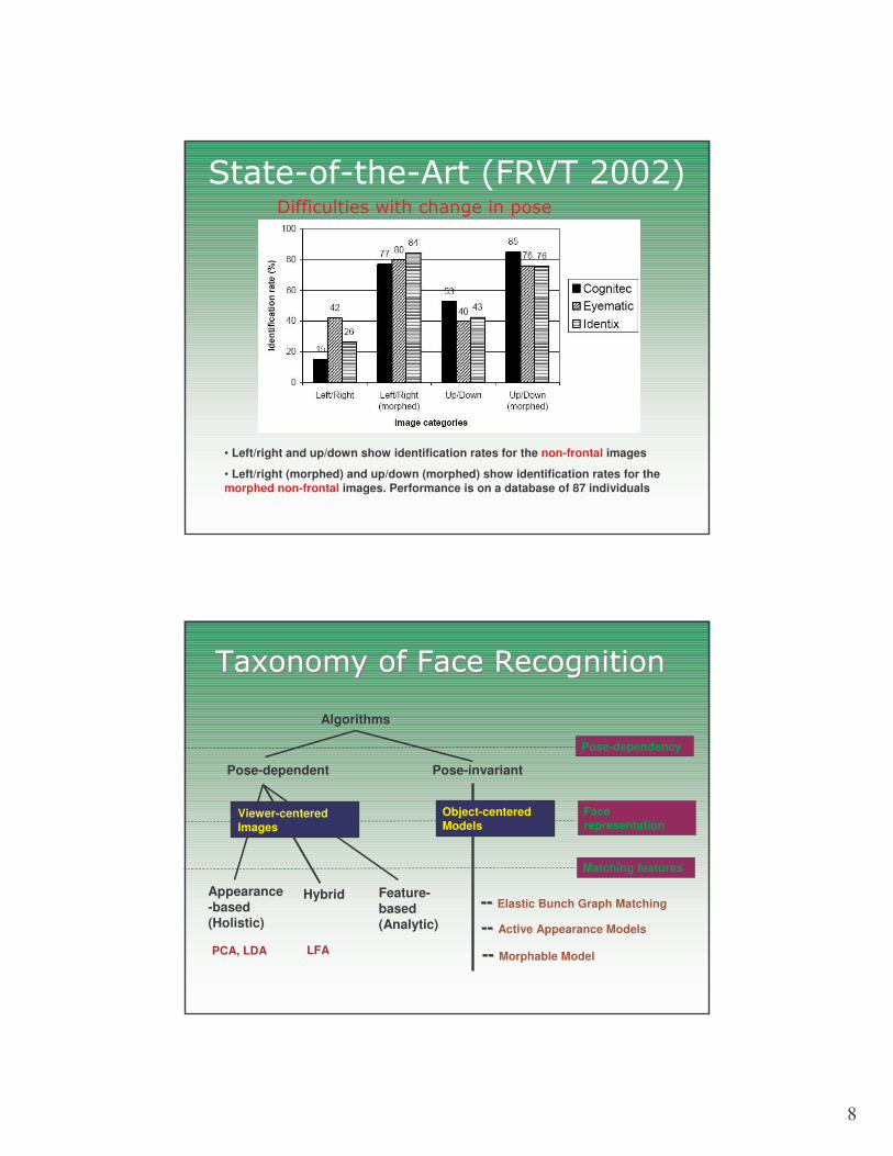
• Left/right and up/down show identification rates for the non-frontal images

• Left/right (morphed) and up/down (morphed) show identification rates for the morphed non-frontal images. Performance is on a database of 87 individuals

-��

Pose-dependent

Algorithms

Pose-invariant

Pose-dependency

Matching features

Appearance-based (Holistic)

---- Elastic Bunch Graph MatchingFeature-based (Analytic)

Hybrid

Viewer-centered Images

---- Active Appearance Models

Object-centered Models

---- Morphable Model

Face representation

PCA, LDA LFA

.�,��+�� .�,��+��

9

Analytic Approach

][ 12,3,2,1 ddddx �=

Analytic Example

Can be difficult to obtain reliable and repeatable anchor points.

10

Holistic Approach

95 100 104 110 113 115 116 . . . 119 121

c

r ][ ),1(),71(),61(),51(),41(),31(,),2,1(),1,1( ,,,,, cpppppppp �

1),()2,2()1.2(),1()3,1()2,1()1,1( ],[ ,,,,,, dxcrc pppppppx ��=One long vector of size d = r×c

Dealing With Large Dimensional Spaces

• Curse of Dimensionality• Every point in the d dimensional space is a

picture• The majority of the points are just noise• Goal is to identify the region of this space

with points that are faces

11

Principal Components (2D Example)

V1V2

Principal Component Analysis(a.k.a Karhunen-Loeve Projection)

• Given n training images x1, x2, x3, … , xn

• Where each xi is a d-dimensional column vector• Define the image mean as:

• Shift all images to the mean:

• Define d×d Covariance Matrix on set X as:

�=

=n

iii x

n 1

1µ

iii xu µ−= dxnnuuuuU ],[ ,3,2,1 �=

Tx UUC =

12

Computation of Principal Component Axes

• Goal, Calculate eigenvectors Vi such that:

• The scatter matrix could be quite large– How big is a scatter matrix with 240 rows × 320 cols?

• Solving for a large scatter matrix is difficult• We need to use a linear algebra method to solve a

much smaller matrix• The following matrix is much smaller than the scatter

matrix as long as n < d:

iiiT VVUU λ=

UU T

Efficient Eigenvector Calculation

• Calculate the eigenvectors (Wi) of this new matrix:

• It can be shown that:

• Then let Vi be a unit vector:

• Solving for Wi will give you Vi which is what we want

iiiT WUWU λ=

iiiT UWUUWU λ=

Vi Vi

niUWUW

Vi

ii ,,3,2,1, �==

13

Feature Space Reduction

• Order the eigenvectors based on the magnitude of the eigenvalues

• Find the smallest b such that:

where α is the ratio of information loss (ex: α=0.5)• The b vectors are used to define the new PCA subspace:

αλ

λ≤

�

�

=

+=n

jj

n

bii

1

1

nλλλλ ≥≥≥≥ �111

bVVVV ,,3,2,1 �

Ideallyb << d

Visualizing the Principal Component Axes as an Image

V1 V2 V3

V5V6 V7V4

V9V10 V11V8

V13V14 V15V12

µx

http://vismod.media.mit.edu/vismod/demos/facerec/basic.html

b =15

14

Converting Images to the New PCA Subspace

• Reorder Subspace Vectors in to a matrix:

• Project original image into the new PCA sub-space:

• Reconstruct an approximate original image from a subspace Vector:

)( µ−== iT

iT

i xMUMy

dxbbVVVVM ][ 321 �=

iii xMyx ≈+= µ'

)( µ−== XMUMY TT (Matrix Notation)

Reconstructed Images From M and µx

• Calculate the new image vector xnew.

• Convert image into new subspace ynew.

• Remember, the size of the y vector is less than the size of the x vector

• Reconstruct the original image

Images from: http://vismod.media.mit.edu/vismod/demos/facerec/basic.html

= xnew

)( µ−= newT

new xMy

newnew Myx += µ'

x’new=

15

Problems with PCA(2D Example)

-0.4 -0.3 -0.2 -0.1 0 0.1 0.2 0.3 0.4 0.5 0.6-0.3

-0.2

-0.1

0

0.1

0.2

0.3

0.4

V1V2

Linear Discriminate Analysis

• Uses the class information to choose the best subspace

• Training examples have class labels– Samples of the same class are close together– Samples of different classes are far apart

• Start by calculating the mean and scatter matrix for each class

16

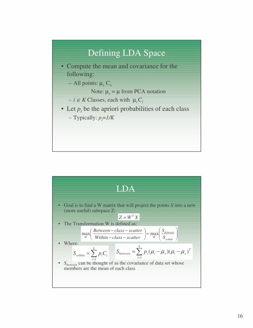
Defining LDA Space• Compute the mean and covariance for the

following:– All points: µx Cx

Note: µx = µ from PCA notation– i ∈ K Classes, each with µi Ci

• Let pi be the apriori probabilities of each class– Typically: pi=1/K

LDA

• Goal is to find a W matrix that will project the points X into a new (more useful) subspace Z:

• The Transformation W is defined as:

• Where:

• Sbetween can be thought of as the covariance of data set whose members are the mean of each class

XWZ T=

��

��

�=�

�

��

�

−−−−

within

between

WW SS

scatterclassWithinscatterclassBetween

maxmax

�=

−−=k

i

Txixiibetween pS

1

))(( µµµµ�=

=k

iiiwithin CpS

1

17

Solving for W

• Goal Maximize the following:

• The optimal projection (W) which maximizes the above formula can be obtained by solving the generalized eigenvalue problem

WSWS withinbetween λ=

��

��

�=�

�

��

�

−−−−

within

between

WW SS

scatterclassWithinscatterclassBetween

maxmax

Review of Linear Transformations• Principal Component Analysis (PCA)

– Calculates a transformation from a d-dimensional space into a new d-dimensional space

– The axes in the new space can be ordered from the most informative to the least informative axis

– Smaller feature vectors can be obtained by only using the most informative of these axes (however some information will be lost)

• Linear Discriminate Analysis (LDA)– Uses the class information to choose the best subspace which

maximizes the between class variation while minimizing the within class variation

Note: both PCA and LDA are general mathematical methods and may be useful on any large dimensional feature space, not just faces or images

18

Lecture Review• There are two general approaches to face

recognition:– Analytic – Holistic

• In the Analytic approach, features are determined by heuristic knowledge of the face

• In the Holistic approach, each pixel in an image can be viewed as a separate feature dimension

• PCA can be used to reduce the size of the feature space

• If the faces are labeled, LDA can be used to find the most discriminating subspace

Recognizing Faces - Michigan State University

Documents

Transcript of Recognizing Faces - Michigan State University