Recent Dynamics of Crude Oil Prices - IMF · Recent Dynamics of Crude Oil Prices ... level of...
30
WP/06/299 Recent Dynamics of Crude Oil Prices Noureddine Krichene
Transcript of Recent Dynamics of Crude Oil Prices - IMF · Recent Dynamics of Crude Oil Prices ... level of...
WP/06/299
Recent Dynamics of Crude Oil Prices
Noureddine Krichene

© 2006 International Monetary Fund WP/06/299 IMF Working Paper African Department
Recent Dynamics of Crude Oil Prices
Prepared by Noureddine Krichene1
Authorized for distribution by Benedicte Vibe Christensen
December 2006
Abstract
This Working Paper should not be reported as representing the views of the IMF. The views expressed in this Working Paper are those of the author(s) and do not necessarily represent those of the IMF or IMF policy. Working Papers describe research in progress by the author(s) and are published to elicit comments and to further debate.
Crude oil prices have been on a run-up spree in recent years. Their dynamics were characterized by high volatility, high intensity jumps, and strong upward drift, indicating that oil markets were constantly out-of-equilibrium. An explanation of the oil price process in terms of the underlying fundamentals of oil markets and world economy was provided, viewing pressure on oil prices mainly as a result of rigid crude oil supply and an expanding world demand for crude oil. A change in the oil price process parameters would require a change in the underlying fundamentals. Market expectations, extracted from call and put option prices, anticipated no change, in the short term, in the underlying fundamentals. Markets expected oil prices to remain volatile and jumpy, and with higher probabilities, to rise, rather than fall, above the expected mean. JEL Classification Numbers: C10 C20 C32 Q4. Keywords: Characteristic function, crude oil, cumulants, drift, Fourier inversion, jump-diffusion,
kurtosis, option pricing, skewness, variance-gamma distribution, volatility. Author’s E-Mail Address: [email protected]; [email protected]; [email protected]
1 The author expresses deep gratitude to Abbas Mirakhor, Abdoulaye Bio-Tchané, Genevieve Labeyrie, Robert Flood, Saeed Mahyoub, U. Jacoby, A. Kovanen, C. Steinberg (all IMF), and Ibrahim Gharbi (the Islamic Development Bank) for their help with this paper.

2
Contents
I. Introduction ............................................................................................................................3
II. Empirical Aspects of futures oil prices during 2002–06.......................................................4 A. Recent Trends and Descriptive Statistics..................................................................4 B. Oil Price Time-Varying Volatility ............................................................................7
III. Crude oil price as a Merton Jump-Diffusion Process ..........................................................9 A. The Stochastic Differential Equation for the Jump-Diffusion Model.......................9 B. Alternative Methods for Estimating the Jump-Diffusion Model: Maximum .........11 Likelihood, Method of Cumulants, and Method of Characteristic Function...............11
IV. Crude Oil Price as a Variance-Gamma Levy Process .......................................................17
V. Option Pricing Using Characteristic Functions ..................................................................19
VI. Density Forecast of Crude Oil Prices: The Inverse Problem.............................................21
VII. Conclusions ......................................................................................................................23
Tables
1. Time-Series Properties of the Oil Price .................................................................................6 2. Jump-Diffusion Model: Parameter Estimates......................................................................15 3. Parameter Estimates of the VG process 1/...........................................................................19
Figures
1a. Oberserved Daily Oil Futures Prices....................................................................................5 1b. Actual and Fitted Oil Price ..................................................................................................5 2. Daily Crude Oil Price Returns ...............................................................................................7 3a. Implied Volatility .................................................................................................................8 3b. Estimated GARCH...............................................................................................................8
Annex
1. Method of Cumulants of Probability Distributions .............................................................24
References
References................................................................................................................................26
3
I. INTRODUCTION
Under the combination of an expanding world demand for crude oil and a tight world crude supply, crude oil prices have been on a run-up spree in recent years. By breaking a record level of US$78.30 per barrel (bl) on August 7, 20062 and remaining comfortably in the neighborhood of US$75/bl during part of 2006, crude oil prices had risen to unexpected territory and seemed boundless. While developments in crude oil prices were being followed closely by economic agents, including traders, investors, speculators, and policy makers, not much was known about the stochastic processes driving these prices. Contrary to stock market indices, for which an abundant and advanced modeling literature now exists, crude oil prices, in spite of their importance, have not been subject to extensive modeling research. Knowledge of their underlying stochastic process is highly relevant not only for pricing derivatives and hedging, but also for policy making and short-term forecasting. This paper addressed the dynamics of daily oil prices during January 2, 2002–July 7, 2006.3 Many striking facts regarding oil markets can be stated at the outset. Foremost, world oil demand pressure kept increasing during this period, causing oil prices to rise by more than threefold, from US$21.13/bl on January, 2002 to US$73.76/bl on July, 7, 2006.4 Second, the noted ascent in oil prices was not monotonic or smooth; oil prices rose, often to a new record, retreated temporarily, then resumed their move to higher record; their movements were dominated by high intensity jumps, indicating that oil markets were constantly out-of-equilibrium. Third, oil price volatilities were excessively high. Measured by the implied volatility, volatility was in the range of 30 percent, implying that oil markets were facing big uncertainties regarding future price developments and were sensitive to small shocks and to news. Finally, market expectations, extracted from crude oil call and put option prices, were right-skewed. More specifically, markets held higher probabilities for further price increases than price decreases. Moreover, markets seemed to expect large upward jumps in oil prices, as reflected by the price and volume of options at strikes in the range of US$75–US$85/bl. When modeled as a jump-diffusion (J-D) process, oil price dynamics were dominated by the discontinuous Poisson jump component compared to the continuous Gaussian diffusion component, showing that oil markets were constantly out-of-equilibrium during the sample period and were sensitive to demand and supply shocks and to news. While the variance of the diffusion component was high and significant, it was surpassed by a still higher and significant variance of the jump component. Both variances, together, illustrated the high
2 When BP shut down the Prudhoe Bay field in Alaska for pipeline maintenance. 3 Futures' contracts on Brent, three-month delivery; the sample contains 1130 observations. The source is Reuters. 4 The recessionary effect of high oil prices has been studied by Hamilton (1983). A considerable literature thereafter has dealt with the relationship between oil shocks and real GDP. By causing a general increase in the price level, an oil shock, ceterus paribus, reduces real cash balances and therefore aggregate demand.
4
volatility of the oil markets. The drift of the diffusion component was, however, very high and significant, indicating that oil prices were strongly influenced by an upward trend. The mean of the jump component was negative; more specifically, sharp upward jumps in oil prices had a temporary restraining effect on oil demand and were followed by a short-lived sequence of price retreats. The mean of the jump component was, however, outweighed by the drift of the diffusion component which kept prices on a rising trajectory. Oil prices were also modeled as a Levy process (LP) with a variance-gamma (VG) distribution. The findings were similar to the J-D model. The drift component was positive and highly significant, establishing that oil prices were constantly pulled by an upward trend. The variance of the VG distribution was significant and high. The parameter controlling for the jump process was high and significant, indicating that oil prices were largely dominated by the jump component and oil markets were constantly out-of-equilibrium. The skewness of the VG distribution was negative, indicating that large upward moves in oil prices triggered a temporary depressing effect on world oil demand, translated into a temporary sequence of small negative jumps in oil prices. However, the upward momentum outweighed the small negative jumps. Turning to market expectations, the implied risk-neutral distribution from call and put option prices, assuming a VG process, showed that market participants held higher probabilities for oil prices to rise, rather than fall, above the futures price, and expected oil prices to remain volatile and dominated by a jump process. The paper is structured as follows. Section I is an introduction. Section II describes the time series properties of oil prices and the empirical distribution of oil price returns. Section III models oil prices as a Merton (1976) J-D process. In Section IV, oil price returns are modeled as a Levy process of the variance-gamma type (Madan and Milne, 1991; and Madan et al., 1998). Section V discusses option pricing in the Fourier space (Carr and Madan, 1999). Section VI presents oil price density forecast based on option prices. Section VII concludes.
II. EMPIRICAL ASPECTS OF FUTURES OIL PRICES DURING 2002–06
A. Recent Trends and Descriptive Statistics
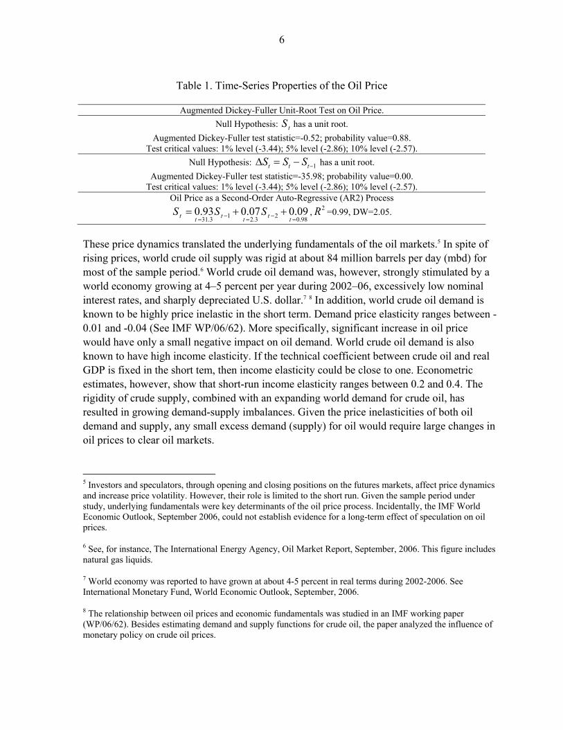
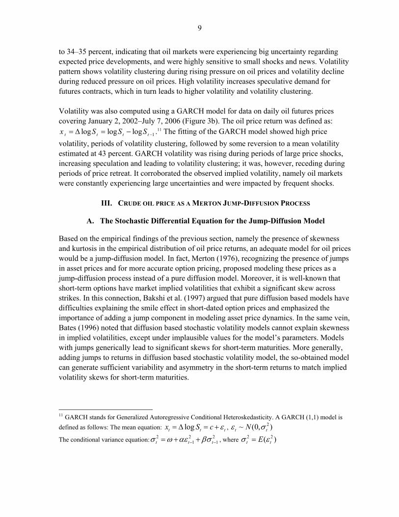
With a view to concentrating on recent oil prices dynamics, the sample period was chosen to be January 2, 2002–July 7, 2006, containing 1130 daily observations. Figure 1a illustrates the daily behavior of oil prices. It clearly shows that oil prices were moving upward, and have become forecastable. After each peak, oil prices seemed to retreat temporarily then re-trended toward a higher peak. Let tS be the oil futures price in US$/bl. An augmented Dickey-Fuller test (Table 1) indicated that tS possessed a unit root; it was pulled by an upward trend, showing no sign for mean reversion. Changes in tS , defined as 1t t tS S S −∆ = − , were, however, stationary. Based on the unit-root test, the dynamics of the oil process were represented by a simple auto-regression of order two (AR2) which yielded good fit and
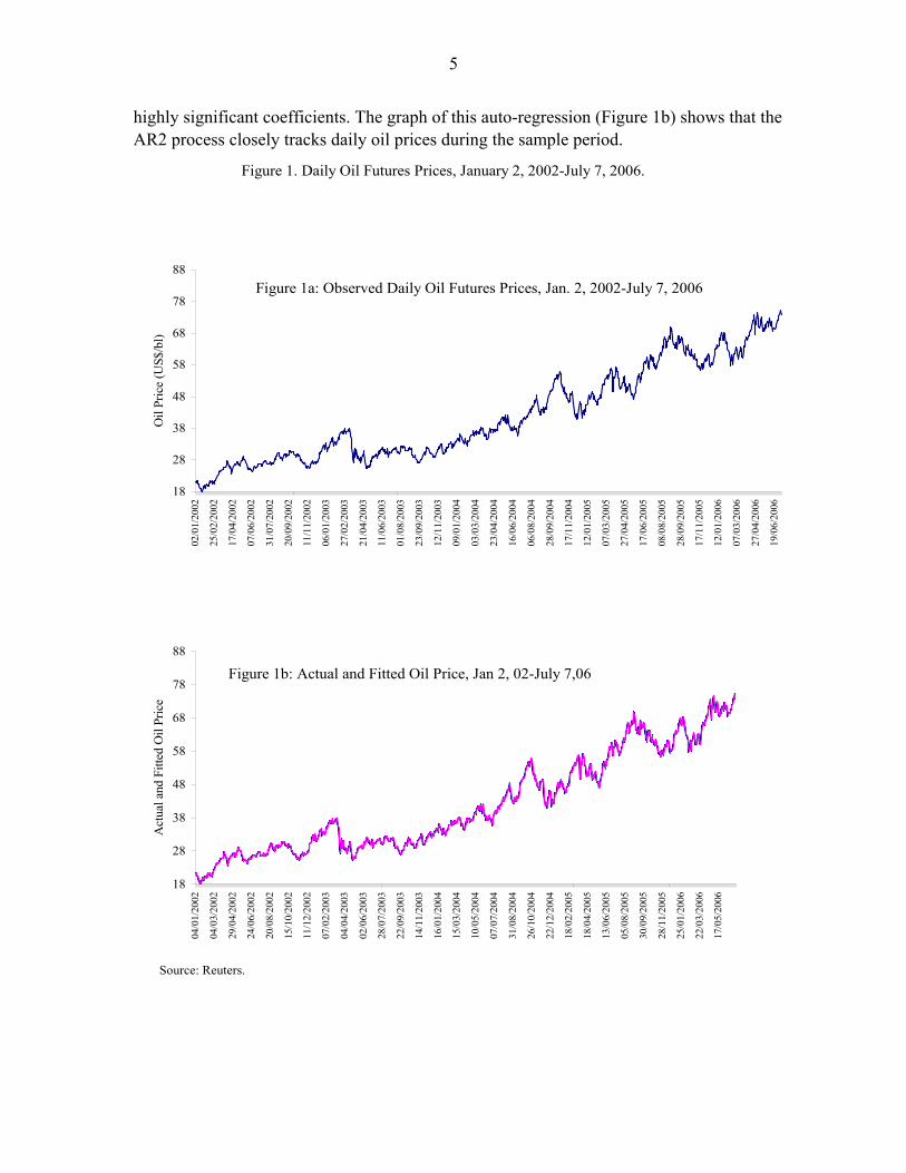
5
highly significant coefficients. The graph of this auto-regression (Figure 1b) shows that the AR2 process closely tracks daily oil prices during the sample period.
Figure 1. Daily Oil Futures Prices, January 2, 2002-July 7, 2006.
Source: Reuters.
Figure 1a: Observed Daily Oil Futures Prices, Jan. 2, 2002-July 7, 2006
18
28
38
48
58
68
78
88
02/0
1/20
02
25/0
2/20
02
17/0
4/20
02
07/0
6/20
02
31/0
7/20
02
20/0
9/20
02
11/1
1/20
02
06/0
1/20
03
27/0
2/20
03
21/0
4/20
03
11/0
6/20
03
01/0
8/20
03
23/0
9/20
03
12/1
1/20
03
09/0
1/20
04
03/0
3/20
04
23/0
4/20
04
16/0
6/20
04
06/0
8/20
04
28/0
9/20
04
17/1
1/20
04
12/0
1/20
05
07/0
3/20
05
27/0
4/20
05
17/0
6/20
05
08/0
8/20
05
28/0
9/20
05
17/1
1/20
05
12/0
1/20
06
07/0
3/20
06
27/0
4/20
06
19/0
6/20
06
Oil
Pric
e (U
S$/b
l)
Figure 1b: Actual and Fitted Oil Price, Jan 2, 02-July 7,06
18
28
38
48
58
68
78
88
04/0
1/20
02
04/0
3/20
02
29/0
4/20
02
24/0
6/20
02
20/0
8/20
02
15/1
0/20
02
11/1
2/20
02
07/0
2/20
03
04/0
4/20
03
02/0
6/20
03
28/0
7/20
03
22/0
9/20
03
14/1
1/20
03
16/0
1/20
04
15/0
3/20
04
10/0
5/20
04
07/0
7/20
04
31/0
8/20
04
26/1
0/20
04
22/1
2/20
04
18/0
2/20
05
18/0
4/20
05
13/0
6/20
05
05/0
8/20
05
30/0
9/20
05
28/1
1/20
05
25/0
1/20
06
22/0
3/20
06
17/0
5/20
06
Act
ual a
nd F
itted
Oil
Pric
e
6
Table 1. Time-Series Properties of the Oil Price
Augmented Dickey-Fuller Unit-Root Test on Oil Price.
Null Hypothesis: tS has a unit root. Augmented Dickey-Fuller test statistic=-0.52; probability value=0.88.
Test critical values: 1% level (-3.44); 5% level (-2.86); 10% level (-2.57). Null Hypothesis: 1t t tS S S −∆ = − has a unit root.
Augmented Dickey-Fuller test statistic=-35.98; probability value=0.00. Test critical values: 1% level (-3.44); 5% level (-2.86); 10% level (-2.57).
Oil Price as a Second-Order Auto-Regressive (AR2) Process
1 231.3 2.3 0.980.93 0.07 0.09t t tt t t
S S S− −= = == + + , 2R =0.99, DW=2.05.
These price dynamics translated the underlying fundamentals of the oil markets.5 In spite of rising prices, world crude oil supply was rigid at about 84 million barrels per day (mbd) for most of the sample period.6 World crude oil demand was, however, strongly stimulated by a world economy growing at 4–5 percent per year during 2002–06, excessively low nominal interest rates, and sharply depreciated U.S. dollar.7 8 In addition, world crude oil demand is known to be highly price inelastic in the short term. Demand price elasticity ranges between -0.01 and -0.04 (See IMF WP/06/62). More specifically, significant increase in oil price would have only a small negative impact on oil demand. World crude oil demand is also known to have high income elasticity. If the technical coefficient between crude oil and real GDP is fixed in the short tem, then income elasticity could be close to one. Econometric estimates, however, show that short-run income elasticity ranges between 0.2 and 0.4. The rigidity of crude supply, combined with an expanding world demand for crude oil, has resulted in growing demand-supply imbalances. Given the price inelasticities of both oil demand and supply, any small excess demand (supply) for oil would require large changes in oil prices to clear oil markets.
5 Investors and speculators, through opening and closing positions on the futures markets, affect price dynamics and increase price volatility. However, their role is limited to the short run. Given the sample period under study, underlying fundamentals were key determinants of the oil price process. Incidentally, the IMF World Economic Outlook, September 2006, could not establish evidence for a long-term effect of speculation on oil prices.
6 See, for instance, The International Energy Agency, Oil Market Report, September, 2006. This figure includes natural gas liquids.
7 World economy was reported to have grown at about 4-5 percent in real terms during 2002-2006. See International Monetary Fund, World Economic Outlook, September, 2006.
8 The relationship between oil prices and economic fundamentals was studied in an IMF working paper (WP/06/62). Besides estimating demand and supply functions for crude oil, the paper analyzed the influence of monetary policy on crude oil prices.
7
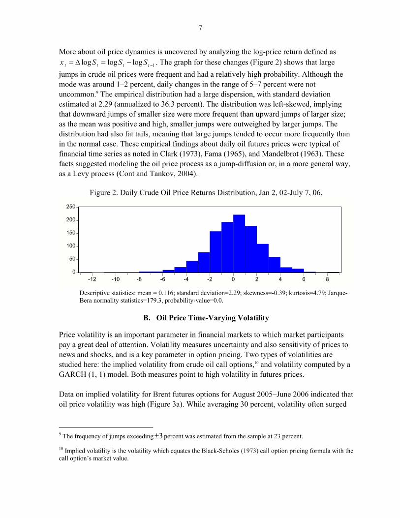
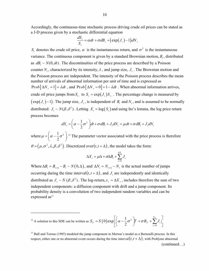
More about oil price dynamics is uncovered by analyzing the log-price return defined as 1log log logt t t tx S S S −= ∆ = − . The graph for these changes (Figure 2) shows that large
jumps in crude oil prices were frequent and had a relatively high probability. Although the mode was around 1–2 percent, daily changes in the range of 5–7 percent were not uncommon.9 The empirical distribution had a large dispersion, with standard deviation estimated at 2.29 (annualized to 36.3 percent). The distribution was left-skewed, implying that downward jumps of smaller size were more frequent than upward jumps of larger size; as the mean was positive and high, smaller jumps were outweighed by larger jumps. The distribution had also fat tails, meaning that large jumps tended to occur more frequently than in the normal case. These empirical findings about daily oil futures prices were typical of financial time series as noted in Clark (1973), Fama (1965), and Mandelbrot (1963). These facts suggested modeling the oil price process as a jump-diffusion or, in a more general way, as a Levy process (Cont and Tankov, 2004).
Figure 2. Daily Crude Oil Price Returns Distribution, Jan 2, 02-July 7, 06.
0
50
100
150
200
250
-12 -10 -8 -6 -4 -2 0 2 4 6 8
Descriptive statistics: mean = 0.116; standard deviation=2.29; skewness=-0.39; kurtosis=4.79; Jarque-Bera normality statistics=179.3, probability-value=0.0.
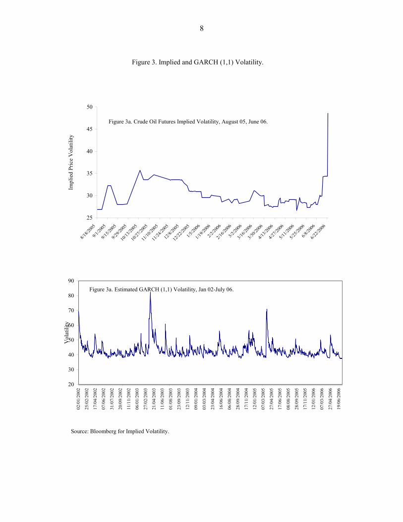
B. Oil Price Time-Varying Volatility
Price volatility is an important parameter in financial markets to which market participants pay a great deal of attention. Volatility measures uncertainty and also sensitivity of prices to news and shocks, and is a key parameter in option pricing. Two types of volatilities are studied here: the implied volatility from crude oil call options,10 and volatility computed by a GARCH (1, 1) model. Both measures point to high volatility in futures prices. Data on implied volatility for Brent futures options for August 2005–June 2006 indicated that oil price volatility was high (Figure 3a). While averaging 30 percent, volatility often surged
9 The frequency of jumps exceeding 3± percent was estimated from the sample at 23 percent.
10 Implied volatility is the volatility which equates the Black-Scholes (1973) call option pricing formula with the call option’s market value.
8
Figure 3. Implied and GARCH (1,1) Volatility.
Source: Bloomberg for Implied Volatility.
Figure 3a. Crude Oil Futures Implied Volatility, August 05, June 06.
25
30
35
40
45
50
8/18/2
005
9/1/20
05
9/15/2
005
9/29/2
005
10/13
/2005
10/27
/2005
11/10
/2005
11/24
/2005
12/8/
2005
12/22
/2005
1/5/20
06
1/19/2
006
2/2/20
06
2/16/2
006
3/2/20
06
3/16/2
006
3/30/2
006
4/13/2
006
4/27/2
006
5/11/2
006
5/25/2
006
6/8/20
06
6/22/2
006
Impl
ied
Pric
e V
olat
ility
Figure 3a. Estimated GARCH (1,1) Volatility, Jan 02-July 06.
20
30
40
50
60
70
80
90
02/0
1/20
02
25/0
2/20
02
17/0
4/20
02
07/0
6/20
02
31/0
7/20
02
20/0
9/20
02
11/1
1/20
02
06/0
1/20
03
27/0
2/20
03
21/0
4/20
03
11/0
6/20
03
01/0
8/20
03
23/0
9/20
03
12/1
1/20
03
09/0
1/20
04
03/0
3/20
04
23/0
4/20
04
16/0
6/20
04
06/0
8/20
04
28/0
9/20
04
17/1
1/20
04
12/0
1/20
05
07/0
3/20
05
27/0
4/20
05
17/0
6/20
05
08/0
8/20
05
28/0
9/20
05
17/1
1/20
05
12/0
1/20
06
07/0
3/20
06
27/0
4/20
06
19/0
6/20
06
Vol
atili
ty
9
to 34–35 percent, indicating that oil markets were experiencing big uncertainty regarding expected price developments, and were highly sensitive to small shocks and news. Volatility pattern shows volatility clustering during rising pressure on oil prices and volatility decline during reduced pressure on oil prices. High volatility increases speculative demand for futures contracts, which in turn leads to higher volatility and volatility clustering. Volatility was also computed using a GARCH model for data on daily oil futures prices covering January 2, 2002–July 7, 2006 (Figure 3b). The oil price return was defined as:
1log log logt t t tx S S S −= ∆ = − .11 The fitting of the GARCH model showed high price volatility, periods of volatility clustering, followed by some reversion to a mean volatility estimated at 43 percent. GARCH volatility was rising during periods of large price shocks, increasing speculation and leading to volatility clustering; it was, however, receding during periods of price retreat. It corroborated the observed implied volatility, namely oil markets were constantly experiencing large uncertainties and were impacted by frequent shocks.
III. CRUDE OIL PRICE AS A MERTON JUMP-DIFFUSION PROCESS
A. The Stochastic Differential Equation for the Jump-Diffusion Model
Based on the empirical findings of the previous section, namely the presence of skewness and kurtosis in the empirical distribution of oil price returns, an adequate model for oil prices would be a jump-diffusion model. In fact, Merton (1976), recognizing the presence of jumps in asset prices and for more accurate option pricing, proposed modeling these prices as a jump-diffusion process instead of a pure diffusion model. Moreover, it is well-known that short-term options have market implied volatilities that exhibit a significant skew across strikes. In this connection, Bakshi et al. (1997) argued that pure diffusion based models have difficulties explaining the smile effect in short-dated option prices and emphasized the importance of adding a jump component in modeling asset price dynamics. In the same vein, Bates (1996) noted that diffusion based stochastic volatility models cannot explain skewness in implied volatilities, except under implausible values for the model’s parameters. Models with jumps generically lead to significant skews for short-term maturities. More generally, adding jumps to returns in diffusion based stochastic volatility model, the so-obtained model can generate sufficient variability and asymmetry in the short-term returns to match implied volatility skews for short-term maturities.
11 GARCH stands for Generalized Autoregressive Conditional Heteroskedasticity. A GARCH (1,1) model is defined as follows: The mean equation: logt t tx S c ε= ∆ = + , 2~ (0, )t tNε σ
The conditional variance equation: 2 2 21 1t t tσ ω αε βσ− −= + + , where 2 2( )t tEσ ε=
10
Accordingly, the continuous-time stochastic process driving crude oil prices can be stated as a J-D process given by a stochastic differential equation
( )( )exp 1tt t t
t
dS dt dB J dNS
α σ= + + −
tS denotes the crude oil price, α is the instantaneous return, and 2σ is the instantaneous variance. The continuous component is given by a standard Brownian motion, tB , distributed as ~ (0, )tdB N dt . The discontinuities of the price process are described by a Poisson counter tN , characterized by its intensity,λ , and jump size, tJ . The Brownian motion and the Poisson process are independent. The intensity of the Poisson process describes the mean number of arrivals of abnormal information per unit of time and is expressed as
[ ]Pr 1tob N dtλ∆ = = , and [ ]Pr 0 1tob N dtλ∆ = = − . When abnormal information arrives,
crude oil price jumps from tS − to ( )expt t tS J S −= . The percentage change is measured by
( )( )exp 1tJ − . The jump size, tJ , is independent of tB and tN , and is assumed to be normally
distributed: 2~ ( , )tJ N β δ . Letting ( )logt tX S= and using Ito’s lemma, the log price return process becomes
212t t t t t t tdX dt dB J dN dt dB J dNα σ σ µ σ⎛ ⎞= − + + = + +⎜ ⎟
⎝ ⎠
where 212
µ α σ⎛ ⎞= −⎜ ⎟⎝ ⎠
.12 The parameter vector associated with the price process is therefore
( )2 2, , , ,θ µ σ λ β δ= . Discretized over ( )∆+tt, , the model takes the form:
0
tN
t t ii
X B Jµ σ∆
=
∆ = ∆ + ∆ +∑
Where ( )~ 0,t t tB B B N+∆∆ = − ∆ , and t t tN N N+∆∆ = − is the actual number of jumps
occurring during the time interval ( )∆+tt, , and iJ are independently and identically
distributed as 2~ ( , )iJ N β δ . The log-return, t tx X= ∆ , includes therefore the sum of two independent components: a diffusion component with drift and a jump component. Its probability density is a convolution of two independent random variables and can be expressed as13
12 A solution to this SDE can be written as ( ) 2
0
10 exp2
TN
T T ii
S S T B Jα σ σ=
⎡ ⎤⎛ ⎞= − + +⎜ ⎟⎢ ⎥⎝ ⎠⎣ ⎦
∑
13 Ball and Torous (1985) modeled the jump component in Merton’s model as a Bernoulli process. In this respect, either one or no abnormal event occurs during the time interval ( )∆+tt, , with Prob[one abnormal
(continued…)
11
( )( )
( )( )
2
2 22 20
( ) 1 exp! 22
n
i
x nef xn nn
λ µ βλσ δπ σ δ
− ∆∞
=
⎡ ⎤⎛ ⎞− ∆ −∆ ⎢ ⎥⎜ ⎟= −⎢ ⎥⎜ ⎟∆ +∆ + ⎝ ⎠⎣ ⎦
∑
With 0,1,2,.......n = . Putting 1=∆ , i.e., the time interval is ( )1, +tt , the density function becomes
( )( )
( )( )
2
2 22 20
( ) 1 exp! 22
n
i
x nef xn nn
λ µ βλσ δπ σ δ
−∞
=
⎡ ⎤⎛ ⎞− −⎢ ⎥⎜ ⎟= −⎢ ⎥⎜ ⎟++ ⎝ ⎠⎣ ⎦
∑
B. Alternative Methods for Estimating the Jump-Diffusion Model: Maximum Likelihood, Method of Cumulants, and Method of Characteristic Function
1. The maximum likelihood method: Let { }Txxxx ,.......,, 21= be an observed sample of log returns, the log-likelihood function can be expressed as:
( ) ( )2
2 22 21 0
1; ln(2 ) ln exp2 ! 2( )
nTt
t j
x nTL x Tn nn
µ βλθ λ πσ δσ δ
∞
= =
⎡ ⎤⎛ ⎞− − −⎢ ⎥= − − + ⎜ ⎟
⎜ ⎟+⎢ ⎥+ ⎝ ⎠⎣ ⎦∑ ∑
Application of the maximum likelihood (ML) method for estimating the J-D model has met with difficulties arising mainly from the identification of the jump parameter and instability of parameter estimates. Nonetheless, Ball and Torous (1983) applied directly the ML method by truncating the number of jumps at 15n = . Ball and Torous (1985) and Jorion (1988) applied the ML method by assuming a Bernoulli process for the jump component. While the ML estimates achieve the lower bound for Cramer-Rao efficiency criterion, difficulties with the likelihood function arising from computational tractability, un-boundedness over the parameter space, and instability of parameters, have led researchers to explore alternative estimation methods, based essentially on the method of moments. 2. The method of cumulants (See Annex I): Press (1967) used the method of cumulants as described in Kendall and Stuart (1977) to estimate the J-D model. Define the characteristic function (CF) of tX as ( ) ( ) ( ) ( )exp expX t t t tu E iuX iuX f X dXφ = =⎡ ⎤⎣ ⎦ ∫ ,
where ( )tf X is the probability density function of tX , u is the transform variable,
event]= ∆λ , Prob[no abnormal event]= ∆− λ1 , and Prob[more than one abnormal event]=0. The density
function for the log-return becomes: ( ) ( )( ) ( )( )2 2 2, , 1f x N n n Nµ β σ δ λ µ σ λ= ∆ + ∆ + ∆ + ∆ ∆ − ∆
12
and 1 i− = .14 The cumulants of tX , denoted by nκ , 0,1,2,....n = , are the coefficients in the power series expansion of the logarithm of the CF of tX , expressed as:
( ) ( ) ( ) ( ) ( )2
1 21
ln 1 ...... ........! 1! 2! !
n n
n nn
iu iu iu iuu
n nφ κ κ κ κ
∞
=
= = + + + + +∑
Noting that the CF for the jump-diffusion process is given by:15
( )1
2 2 2 2
exp exp 12 2Xu uu i u i uσ δφ µ λ β
⎡ ⎤⎛ ⎞⎛ ⎞= − + + − −⎢ ⎥⎜ ⎟⎜ ⎟
⎢ ⎥⎝ ⎠⎝ ⎠⎣ ⎦;
It follows that the first four cumulants of the J-D process are 1κ µ λβ= + , 2 2 2
2κ σ λδ λβ= + + , ( )2 23 3κ λβ δ β= + , ( )4 2 2 4
4 3 6κ λ δ β δ β= + + . Obviously, the
cumulants enable to recover the parameters of the J-D process from sample moments. Press (1967), in order to avoid using higher order cumulants, imposed the restriction 0µ = and
derived the following relations:2
4 23 342
1 1 1
3ˆ ˆ ˆ2 02 2
κ κκβ β βκ κ κ
− + − = , 1ˆˆκλβ
= ,2
2 3 1
1
ˆˆ3
κ β κδκ−
= ,
22 2 3 11
21
ˆˆˆ ˆ 3κ β κκσ κ β
κβ
⎛ ⎞−= − +⎜ ⎟⎜ ⎟
⎝ ⎠. Press’ estimates were often wrong-signed and not plausible.
Beckers (1981) adopted the same method as Press, however, settingβ , instead ofµ , to zero. Using sixth order cumulant, his cumulant equations yielded the following system: 1µ̂ κ= ,
34
26
25ˆ3κλκ
= , 2 6
4
ˆ5κδκ
= , and 2
2 42
6
5ˆ3κσ κκ
= −
Beckers’ estimates improved those of Press, yet they were not free of anomalies. Ball and Torous (1983), using a Bernoulli, instead of a Poisson, jump process and maintaining Beckers’ restriction, i.e. 0β = , derived the following cumulant equations: 1κ µ= ,
2 22κ σ λδ= + , 3 0κ = , ( )2
4 3 1κ δ λ λ= − , 5 0κ = , and ( )( )66 15 1 1 2κ δ λ λ λ= − − . Again by
equating with population cumulants, they obtained estimators µ̂ , λ̂ , 2σ̂ , and 2δ̂ given by:
1µ̂ κ= , ( )* *ˆ 1 3 /(3 100) / 2λ κ κ= ± + , where ( )2*6 4/κ κ κ= , 2 2
2ˆ ˆσ̂ κ λδ= − , and
( )( )( )26 4
ˆ ˆ/ 5 1 2δ κ κ λ= − .
14 The characteristic function ( )X uφ is related to the moment generating function ( )XG u
( ) ( ) ( ) ( )exp expX t t tG u E uX uX dF X= =⎡ ⎤⎣ ⎦ ∫ by a change of the transform variable u iu→− ,
namely ( ) ( )X XG iu uφ= , and ( ) ( )X XG u iuφ= − .
15 See, for instance, Madan and Seneta (1987), and Cont and Tankov (2004).
13
Das and Sundaram (1999) used the method of moments to estimate the J-D model. Denoting the log-price return by tx , and assuming that the jump size tJ is distributed as
( )2~ ,J N β δ , they showed that the first moments of the J-D process are given by the
following equations which they used to estimate the model’s parameters; however, for the Poisson parameterλ , they imposed a given value.
[ ] ( )( ) ( )2 2 2Var x E x E x σ λδ⎡ ⎤= − = +⎣ ⎦
( )( )( )
( )( )
( )
33 2
3/ 2 3/ 22 2 2
3E x E xskewness x
Var x
λ β βδ
σ λδ λβ
⎡ ⎤− +⎣ ⎦= =⎡ ⎤ + +⎣ ⎦
( )( )( )
( )( )( )
44 2 2 4
2 22 2 2
6 33
E x E xkurtosis x
Var x
λ β β δ δ
σ λδ λβ
⎡ ⎤− + +⎣ ⎦= = +⎡ ⎤ + +⎣ ⎦
3. The method of the characteristic function (CF): As there is a one-to-one correspondence between the CF, ( ) ( ) ( ) ( )exp expX t t t tu E iuX iuX f X dXφ = =⎡ ⎤⎣ ⎦ ∫ , and the
corresponding probability density, ( )tf X , the CF conveys the same information as the probability distribution. Often, the transition density function of a stochastic process may not be available in closed form, while the CF is readily available in closed form. Knowledge of the analytic form of the CF allows estimating the parameters of the process by the method of moments or the empirical CF procedure (ECF). 16 The method of moments computes non-
central moments of any order n as ( ) ( ) 01 |
nn
t un n
dE X ui du
φ =⎡ ⎤ =⎣ ⎦ . It also enables the
application of the empirical characteristic function method (ECF). In both cases, a General Method of Moments (GMM) procedure is implemented, consisting of minimizing a distance norm between the sample and the theoretical population moments, or the sample CF and the theoretical CF. The exact method of moments consists of estimating the parameter vector
which minimizes the distance ( ) 01 |
nn
un nE Xi u
φ=
∂−
∂.17
16 Parzen (1962), Feuerverger and Mureika (1977), Feuerverger and McDunnough (1981a and 1981b)) suggested the use of the CF to deal with the estimation of density functions. Madan and Seneta (1987) proposed a CF-based approach to estimate the J-D model. In the same vein, Bates (1996), Duffie et al. (2000), Chacko and Viceira (2003), and many other authors have proposed the use of CF for estimating affine J-D models. 17 Note that ( ) ( )log log
nX n XnX e e= = . Therefore,
( ) ( ) ( )( ) ( ) ( ) ( ) ( )nLog X nLog X nLog Xn
Log XE X E e E e e f X dX nφ∞
−∞
⎛ ⎞= = = =⎜ ⎟⎝ ⎠ ∫ . Namely, for the log-
(continued…)
14
The ECF method can be described as follows. Suppose { }Txxxx ,.......,, 21= is an identically independently distributed realization of the same variable X with density ( ; )f x θ and a distribution ( )F xθ . The parameter lRθ ∈ is the parameter of interest with true value 0θ . It is to
be estimated from { }Txxxx ,.......,, 21= . Define the theoretical CF as: ( ) ( ; )iuxu e f x dxθφ θ= ∫
and its empirical counterpart (ECF) as
1 1 1
1 1 1( ) ( ) exp( ) cos( ) sin( )n n n
iuxn n j j j
j j
u e f x dx iux ux i uxT T T
φ= =
= = = +∑ ∑ ∑∫
The ECF procedure consists of estimating θ according to the criterion 'ˆ arg min( ) ( )n nWθ θθ
θ φ φ φ φ= − −
W is a positive semi-definite matrix. Because the minimization of the distance between the ECF ( )nφ and CF ( )θφ over a grid of points in the Fourier domain is equivalent to matching a finite number of moments, the ECF method is in essence equivalent to the Generalized Method of Moments (GMM). Feuerverger (1990) proved that, under some regularity conditions, the resulting estimates can be made to have arbitrarily high asymptotic efficiency provided that the sample of observations is sufficiently large and the grid of points is sufficiently fine and extended. Indeed, ECF estimators have the same consistency and asymptotic efficiency as the GMM estimators. Moreover, when the number of orthogonal conditions exceeds the number of parameters to be estimated ( )r l> , the model is over-identified, in that more orthogonal conditions are used than needed to estimate θ . A test of over-identifying restrictions may be used. In this respect, Hansen (1982) suggested a test of whether all of the sample moments are as close to zero as would be expected if the corresponding population moments were truly zero. 4. Empirical results of the estimation Based on a sample of daily prices for Brent futures prices described in Section II, alternative methods were used for estimating the J-D model (Table 2). First, assuming a Bernoulli jump process, the ML was applied unrestrictedly, and with restriction on the probabilityλ of a jump occurring on a trading day given byλ =0.23. Second, the method of cumulants was applied consecutively with restrictionsλ =0.23, µ =0 (Press, 1967), and β =0 (Beckers, 1981), respectively. The third method was the ECF applied unrestrictedly and with restriction
return 1log( / )t t tx S S −= , ( ) ( )( ) ( ) ( ) ( )1/ nt tlog S Sn nx nx
xE x E e E e e f X dX nφ−
∞
−∞
= = = =∫ . It follows that
the n th− order moment ( )nE x can be computed by replacing the transform variable u by n in the CF of
( )1log /t t t tx X S S −= ∆ = .
15
λ =0.23. The three methods yielded parameter estimates that were consistent with the empirical features of oil prices discussed in Section II. They showed pointedly that the dynamics of the oil price process were influenced by both diffusion and jump components; however the jump component was the dominant one. Besides having high intensity, the jump component had a much higher variance than the diffusion component. The high variance of the jump component illustrated the presence of jumps of large magnitude and was in conformity with the excess kurtosis in the empirical distribution of oil price returns. The mean of the jump size tended to be negative, in conformity with the negative skewness of the empirical distribution. This was due to the fact that crude oil prices were not monotonic; they leapt forward, than retreated back in smaller movements before taking a new jump. The drift of the diffusion component was high, in conformity with the observed upward trend in crude oil prices; it illustrated the presence of a force that kept pushing oil prices upward and was able to outweigh the negative mean of the jump component.
Table 2. Jump-Diffusion Model: Parameter Estimates
Methods Driftµ Variance 2σ Intensity λ Mean β Variance 2δ Bernoulli process Maximum Likelihood Maximum Likelihood 1/
0.23
(t=3.22) 0.27
(t=3.08)
4.46
(t=20.25) 3.34
(t=14.49)
0.59
(t=1.89) 0.23
-1.12
(t=-4.27) -0.68
(t=-1.93)
4.47
(t=17.12) 7.98
(t=6.25) Cumulants 1/ Press (1967) 2/ Beckers (1981) 3/
0.32 0
0.12
1.81 6.54 3.34
0.23 0.10 0.22
-0.85 1.11
0
2.78 -13.88 8.62
ECF 4/ ECF 1/ 4/
0.57 (t=7.96)
0.27 (t=16.1)
0.54 (t=1.11) 3.45
(t=127)
4.37 (t=3.49)
0.23
-0.10 (t=-6.25)
-0.52 (t=-3.75)
0.96 (t=5.57) 6.97
(t=31.35)
1/ Restriction on 0.23λ = , computed from the data sample as the frequency of a jump in the crude oil price exceeding ± 3 percent. 2/ Restriction on µ =0. 3/ Restriction on β =0. 4/ The grid for u consists of twenty points: 0.1,0.2,0.3,........,1.9,2.0. Assuming a Bernoulli jump process, the ML estimates were highly significant and stable. The drift of the diffusion component, estimated at µ̂ =0.23, was very high and significant, showing that oil prices were constantly under pressure to move upward. The variances of the diffusion and jump components were high and significant, 2σ̂ =4.46 and 2δ̂ =4.47, respectively. The variance of the jump component became more important than that of the diffusion component when the jump intensity was restricted to λ =0.23. The probability of a jump in the unrestricted case, computed at λ̂ =0.59, was high and borderline significant. The mean of the jump component, estimated at β̂ =-1.12, was negative and consistent with the negative skewness observed in the data. Oil prices tended to make large moves upward, then started to retreat through a sequence of smaller and frequent negative jumps, until they were shocked again, making new jumps forward. Yet, the significance of the drift of the diffusion

16
process was such that the smaller negative jumps could not outweigh the strong momentum that kept pushing oil prices upward. The method of cumulants was applied under alternative restrictions. The restrictionλ =0.23 yielded results that were similar to the ML under the same restriction. The drift of the diffusion component, estimated at µ̂ =0.32, was very high, showing that oil prices were constantly under pressure to move upward. The variances of the diffusion and jump components, were estimated at 2σ̂ =1.81 and 2δ̂ =2.78, respectively, indicating that the jump component tended to dominate the dynamics of the oil price process. The mean of the jump component, estimated at β̂ =-0.85, was negative and consistent with the negative skewness in oil price returns. Application of the Press (1967) method, with the restrictionµ =0, yielded
implausible results for the variance of the jump component, namely 2δ̂ =-13.88. Such an anomaly was not unexpected in the case of Press’ method, indicating that the restriction µ =0, could not be borne by the data, and was in sharp contrast with the strong upward trend in oil prices. In contrast, Beckers’ method, with the restrictionβ =0, yielded results which were highly plausible. The drift component of the diffusion, estimated at µ̂ =0.12, was smaller than, say, in the ML case, sinceβ =0 implied less influence for the drift of the diffusion, compared to the case whenβ was negative, to maintain an upward trend in oil prices; it was, however, close to the drift of the AR2 (Table 1) and the actual mean of oil price returns (Figure 2). The variances of the diffusion and jump components were high,
2σ̂ =3.34 and 2δ̂ =8.62, respectively. The variance of the jump component, however, dominated that of the diffusion component. Noticeably, the jump intensity, estimated at λ̂ =0.22, was quite close to the frequency of jumps in oil prices exceeding ± 3 percent, computed from the data set.
17
The ECF was applied unrestrictedly and with restrictionλ =0.23. The drift of the diffusion component, estimated at µ̂ =0.57, was very high and significant. The variance of the diffusion component, 2σ̂ =0.54, was not significant, and was dominated by the variance of the jump component, 2δ̂ =0.96, which was significant. The intensity of the jump process, estimated at λ̂ = 4.37, was high and significant, indicating that the oil price process was characterized by frequent jumps. The mean of the jump component, β̂ =-0.1, was negative, significant, and consistent with skewness in oil price returns. The ECF, applied with the restrictionλ =0.23, yielded results which were similar to those of the ML using the same restriction. The drift µ̂ =0.27 was positive and significant; the variance of the diffusion,
2σ̂ =3.34, was significant; however, it was dominated by the variance of the jump component, 2δ̂ =6.97, indicating that the jump process played a more important role in oil price dynamics in relation to the diffusion process. The mean of the jump component, β̂ =-52, was negative, significant and consistent with skewness observed in the data. In sum, parameter estimates from the three methods were fully concordant with the data. They established that the oil price process was dominated by the jump process, with large discontinuities occurring at high intensity, meaning that oil markets were permanently out-of-equilibrium during the sample period. The negative mean of the jump component could be seen as smaller downward adjustment in world crude oil demand following a large upward jump in oil price. However, the downward adjustment in demand was short-lived; the drift component of the diffusion process was very high for daily data, indicating that oil demand was pushed up by a strong income effect; consequently, oil prices were under a constant pressure to move upward. These results can be easily explained in terms of the elasticities of world demand and supply for crude oil. World demand was highly elastic with respect to world income, and highly inelastic with regard to oil prices. Crude supply has been rigid, showing little sensitivity to prices. As world real GDP expanded at 4–5 percent per year during the period under study, it caused world oil demand to expand at similar rate, creating an excess demand for oil. Given the short-term inelasticity of demand and supply with respect to prices, any small excess demand for oil would cause large variation in prices. In turn, large price increases would have small negative effect on oil demand. The negative price effect, however, would be quickly dominated by a positive income effect.
IV. CRUDE OIL PRICE AS A VARIANCE-GAMMA LEVY PROCESS
The J-D model has essentially two limitations. First, it does not capture the notion of time-varying or stochastic volatility. In particular, stochastic volatility is found to have a key role in explaining skewness and leptokurtosis in financial time-series, and in explaining the skew in market implied volatilities. In this respect, skewed distribution can arise either because of correlations between asset prices and volatility shocks, or because of nonzero average jumps. Similarly, excess kurtosis can arise either from volatile volatility or from a substantial jump component. Second, the J-D model is fit to model finite large jumps, and cannot capture
18
infinite small jumps which are similar to small jumps in the diffusion process. With a view to capture the notion of stochastic volatility and modeling small and frequent jumps, while simplifying computational costs, many researchers (e.g., Carr et. al (2002, 2003), Carr and Wu (2004), Cont and Tankov (2004)) have proposed the use of Levy processes for modeling asset prices. Accordingly, oil prices are modeled in this Section as a Levy process.18 More specifically, oil price returns are assumed to follow a Levy process with a variance-gamma distribution. This type of model has a simple CF and is easier to estimate. 1. Definition of the Variance-Gamma process: a variance-gamma ( )VG process is defined as a Brownian motion with drift α and volatilityσ , i.e. tt Bα σ+ , where tB is an ordinary Brownian motion, time-changed by a gamma process. More precisely, let
{ , 0}tG G t= ≥ be a gamma process with mean 1/ 0a υ= > and variance 1/ 0b υ= > .19 Let { , 0}tB B t= ≥ denote a Brownian motion, and let 0σ > and Rα ∈ ; then the VG
process ( ) ( ){ , 0}VG VGtX X t= ≥ , with parameters 0σ > , 0υ > andα , can be defined
as ( )t
VGt t GX G Bα σ= + . The CF is given by
( ) 2 21( ; , , ) [exp( )] (1 )2
tVG
VG tu E iuX iu u υφ σ υ α αυ σ υ−
= = − + . The two additional parameters in
theVG distribution, which are the drift of the Brownian motion,α , and the volatility of the time change,υ , provide control over skewness and kurtosis, respectively. Namely, when 0α < , the distribution is negatively skewed, and vice versa. Moreover, larger values of υ indicate frequent jumps and contribute to fatter tails. The moments of the log-price returns
under ( , , )VG σ υ α are: the mean =α ; the variance = 2 2σ υα+ ; skewness =2 2
2 2 3/ 2
(3 2 )( )
αυ σ υασ υα
++
;
18 A Levy process (LP) 0( )t tX ≥ has a value 0 0X = at 0t = and is characterized by independent and stationary increments, and stochastic continuity, i.e., discontinuity occurs at random times. The CF of a LP is given by the Levy-Khintchine formula:
1
22
1\{0}
( ) [ ] exp [ 1 1 ( )] ( )2
iuX iuxx
R
u E e i u u e iux x dxσφ α ν<
⎛ ⎞= = − + − −⎜ ⎟⎜ ⎟
⎝ ⎠∫ , u R∈ , 0t ≥ . Where
Rα ∈ is the drift parameter, 2 0σ ≥ is the volatility parameter, and ν is a Levy measure on \{0}R , which
measures jumps of different sizes. A LP is characterized by its triplet 2( , , )α σ ν .
19 The probability density of the Gamma process with mean rate t and variance tυ is well
known:1 1
( ) / ( )x t tf x x eυ υ υυ
υ− −
= Γ . Its Laplace transform is [exp( )] (1 )t
tE uG uυ υυ−
− = + .
It results that the VG process has a simple CF2
2( ) 1/(1 )2
t
VG u i u u υσ υφ αυ= − + .
19
and kurtosis = 4 2 2 23(1 2 ( ) )υ υσ σ υα −+ − + . Clearly, skewness is influenced byα , and kurtosis byυ . 2. Estimation of the Variance-Gamma process Let the crude oil price tS be modeled as 0 exp[ ]t tS S t Xµ= + where tX is a VG process. The log price return is 1logt t t tx S X Xµ −= ∆ = + − . The CF of the log price return is
[ ] [ ]1
2 21 1
1[exp( )] exp( ( ) exp( ) exp( ) exp( )(1 )2tE iux E iu X iu E iuX iu i u u υµ µ µ αυ σ υ
−= + = = − +
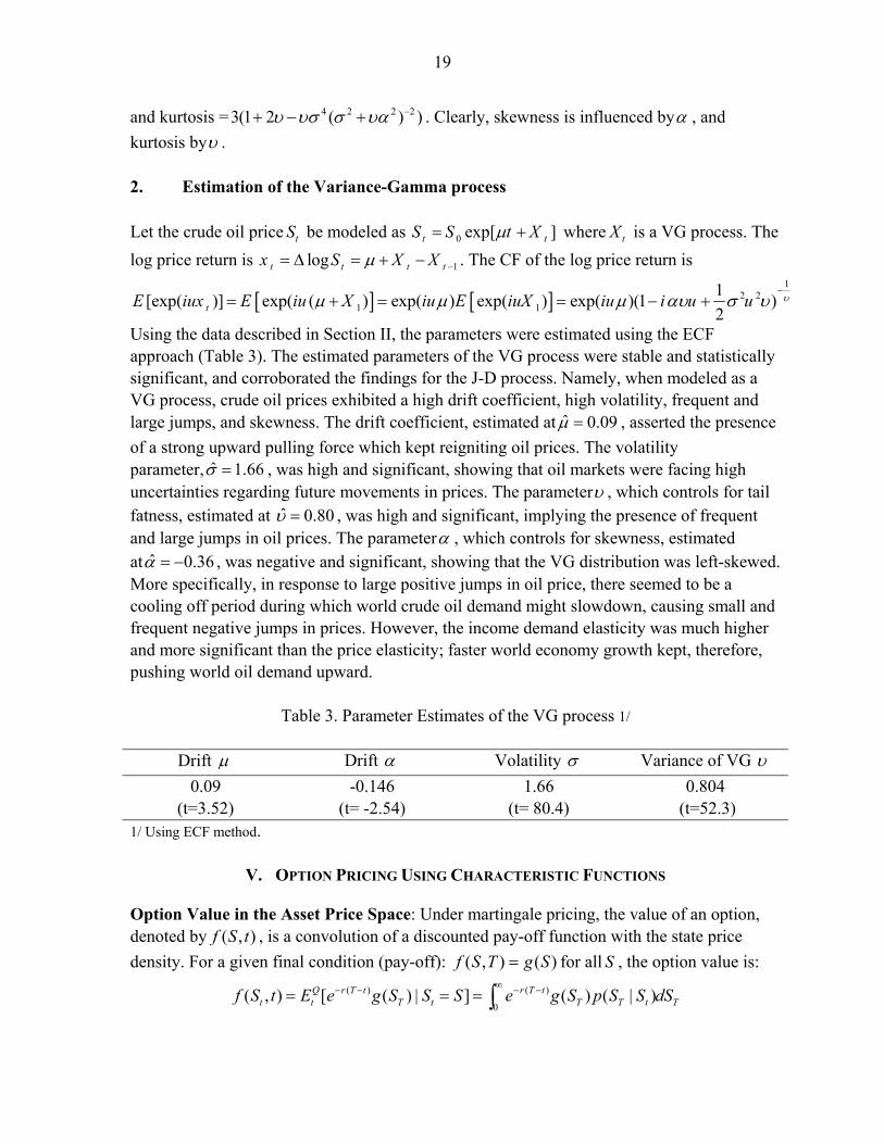
Using the data described in Section II, the parameters were estimated using the ECF approach (Table 3). The estimated parameters of the VG process were stable and statistically significant, and corroborated the findings for the J-D process. Namely, when modeled as a VG process, crude oil prices exhibited a high drift coefficient, high volatility, frequent and large jumps, and skewness. The drift coefficient, estimated at ˆ 0.09µ = , asserted the presence of a strong upward pulling force which kept reigniting oil prices. The volatility parameter, ˆ 1.66σ = , was high and significant, showing that oil markets were facing high uncertainties regarding future movements in prices. The parameterυ , which controls for tail fatness, estimated at ˆ 0.80υ = , was high and significant, implying the presence of frequent and large jumps in oil prices. The parameterα , which controls for skewness, estimated at ˆ 0.36α = − , was negative and significant, showing that the VG distribution was left-skewed. More specifically, in response to large positive jumps in oil price, there seemed to be a cooling off period during which world crude oil demand might slowdown, causing small and frequent negative jumps in prices. However, the income demand elasticity was much higher and more significant than the price elasticity; faster world economy growth kept, therefore, pushing world oil demand upward.
Table 3. Parameter Estimates of the VG process 1/
Drift µ Drift α Volatility σ Variance of VG υ 0.09
(t=3.52) -0.146
(t= -2.54) 1.66
(t= 80.4) 0.804
(t=52.3) 1/ Using ECF method.
V. OPTION PRICING USING CHARACTERISTIC FUNCTIONS
Option Value in the Asset Price Space: Under martingale pricing, the value of an option, denoted by ),( tSf , is a convolution of a discounted pay-off function with the state price density. For a given final condition (pay-off): )(),( SgTSf = for all S , the option value is:
( ) ( )
0( , ) [ ( ) | ] ( ) ( | )Q r T t r T t
t t T t T T t Tf S t E e g S S S e g S p S S dS∞− − − −= = = ∫

20
WhereQ is the risk-neutral measure. The conditional expectation is computed with respect to a risk-neutral transition probability density )|( tT SSp . However, for many stochastic processes involving stochastic volatility, jumps, or Levy type processes, transition densities are often complicated and may not be readily available in closed form. In contrast, the CF of the underlying stochastic process may be readily available in closed form. It is defined as
0( , ) ( | )TiuS
T t Tu t e p S S dSφ∞
= ∫ , u is the transform variable.
Option Value in the Fourier Space: knowledge of the CF enables to compute option prices in the Fourier space according to two alternative methods. The first method, proposed by Heston (1993), relies on a numerical inversion of the CF. However, noting the singularity of Heston’s formula at 0u = , Carr and Madan (1999) proposed, instead, a numerical inversion of the Fourier transform of the option value. More specifically, define the Fourier transform
of the option value as ( ) ( )ˆ iuSf u e f S dS∞
−∞
= ∫ . If ( )f̂ u can be explicitly expressed in terms of
( )uφ as ( ) ( )( )ˆ ˆf u f uφ φ= a fast Fourier transform (FFT) inversion of ( )( )f̂ uφ φ would then
compute the option value from its transform as ( ) ( )1 ˆ,2
iuSf S t e f u duπ
∞−
−∞
= ∫ .
Let lnt ts S= be the log-price; ln( )k K= the log strike price; ( )TC k = value of a T −maturity call option with strike K ; and ( ) exp( ) ( )T Tc k ak C k≡ for 0a > , the damped option price. The
CF of lnt ts S= under the risk-neutral measure is given by ( , ) ( | )TiusT t Tu t e p s s dsφ
∞
−∞= ∫ . Let
( ) ( )iukT Tu e c k dkψ
∞
−∞
= ∫ be the Fourier transform of ( )Tc k . Carr and Madan (1999) showed that
( )T uψ can be expressed in terms of ( )T uφ as: 2 2
( ( 1) )( )(2 1)
rTT
Te u a iu
a a u i a uφψ
− − +=
+ − + +. Knowledge of
the CF ( )T uφ , which is the CF of the log of the asset price under the risk neutral-measure, implies knowledge of the Fourier transform of the value of the option ( )T uψ . The option price can therefore be computed via Fourier inversion as:
0
exp( ) exp( )( ) ( ) ( )2
iuk iukT
ak akC k e u du e u duψ ψπ π
∞ ∞− −
−∞
− −= =∫ ∫ .
Option pricing requires evidently knowledge of the risk-neutral process and the CF associated with this process. Under the risk neutral process, money market account discounted asset prices are martingales and it follows that the mean rate of return on the asset under this probability measure is the continuous compounded risk-free interest rate r . If the asset price tS is modeled as 0 exp[ ]t tS S rt X= + where tX is an LP, to obtain a risk-neutral
21
process verifying the martingale property, define: exp( ( )) exp( )exp( ( ))( ) (0) (0)
[exp( ( )] [exp( ( )]rt X t rt X tS t S S
E X t E X t+
= = , then ( )( ) / exp( ) (0)E S t rt S= . The
resulting risk-neutral process for the log price is: log ( ) (log (0) log [exp( ( )]) ( ))S t S rt E X t X t= + − + . The CF of the log price is:
[exp( log( ( )))] exp( ((log (0) log [exp( ( )]) [exp( ( ))]E iu S t iu S rt E X t E iuX t= + − . For the VG model, the resulting risk-neutral process for the asset price is:
0 exp[ ( , , ) ]t tS S rt X tσ α υ ω= + + , 0t > , where, by setting 21 1( ) ln(1 )2
ω αυ σ υυ
= − − , Madan
et al. (1998) showed that the CF for log of tS is:
2 20
1( ) exp[ln( ) ( ) ](1 )2
t
t u S r t i u u υφ ω αυ σ υ−
= + + − + .
To obtain option prices, one can analytically invert ( )uφ to get the density function and then integrate the density function against the option payoff as in Heston (1993). Alternatively, the Fourier transform of the option value can be numerically inverted using FFT as in Carr and Madan (1999). The Fourier inversion can be approximated discretely via an N -point sum with a grid spacing of ∆ in the Fourier domain. The inversion integral can be approximated using an integration rule, such as Simpson’s or the trapezoidal rule, as
21 ( )
00
( ) jN i j uixu N
jj
e u du eπ
ψ ψ∞ − −−
=
≈ ∆∑∫ % .
The points ju are equidistant with grid spacing ∆ , ju j= ∆ . The value of ∆ should be sufficiently small to approximate the integral well enough, while the value of N∆ should be large enough to assume the CF is equal to zero for u u N> = ∆ . In general, the values jψ% are
set equal to ( )j j ju wψ ψ=% , where jw are the weights of the integration rule.
VI. DENSITY FORECAST OF CRUDE OIL PRICES: THE INVERSE PROBLEM
An application of the above analysis to crude oil options is undertaken in this section with the objective of estimating, from observed options’ market values, density forecast for crude oil prices at a given maturity date. The estimation of the risk-neutral distribution is known as the inverse problem in option pricing models. While the pricing problem is concerned with computing option values given model’s parameters, the inverse problem consists of backing out the parameters describing risk-neutral dynamics from observed prices. The computation of a risk-neutral distribution could be seen as estimating market’s expectations for future prices; in contrast, estimation of statistical distribution from realized data could be seen as the actual distribution of historical prices. Assuming a VG distribution for the log price, the inverse problem can be stated as finding the parameters ( )2, ,θ α σ υ= by minimizing the
quadratic pricing error:
22
( )2*
1
1ˆ arg min ( , ) ( , )N
j j j jj
C T K C T KNθ
θ=
= −∑ , 1, 2,....,j N=
under the put-call parity constraint: ( ) ( )*0 , , rT
j j j j jS P T K C T K K e−+ − =
where * ( , )j jC T K denotes the call option computed from the VG distribution, ( ),j jC T K and
( ),j jP T K denote the observed prices of call and put options for maturity T and strikes jK ,
respectively. ( )* ,j jC T K is given by FFT; namely ( )*
0
exp( ), ( )jiukj
j j T
akC T K e u duψ
π
∞−−
= ∫ .
The addition of the put-call parity condition brings extra-sample information which helps to regularize the estimation problem. 20 Taking into account the put-call parity constraint and choosing a penalty parameter 0h > , the minimization problem becomes
( ) ( ) ( )( )( )22* *0
1
1ˆ arg min ( , ) ( , ) , ,N
rTj j j j j j j j j
jC T K C T K h S P T K C T K K e
Nθθ −
=
= − + + − −∑
The inverse problem was applied for the VG model only for space limitation. The same methodology applies identically to the J-D model.21 The observed data set was for July 21, 2006; it consisted of call and put futures options contracts maturing end-September 2006; the risk-free interest rate, taken here to be the three-month U.S. Treasury bill rate, was equal to 4.965; and the crude futures price, was equal to US$74.43/bl. The constrained minimization yielded the following triplet for the risk-neutral distribution: 2σ̂ = 1.72, υ̂ =1.12, α̂ =0.37 which described market’s expectations on July 21, 2006 regarding futures prices end-September 2006. Clearly, market participants did not anticipate any short-term change in the underlying fundamentals characterizing oil markets. They expected oil prices to remain highly volatile ( 2σ̂ =1.72) and dominated by a jump process (υ̂ = 1.12 ). They also expected oil prices to remain under pressure, as they assigned higher probabilities for oil prices to rise
20 Cont and Tankov (2004) argued that the inverse problem could be an ill-posed problem and proposed the use of relative entropy, which is the Kullback-Leibler distance for measuring the proximity of two equivalent probability measures, as a regularization method with the prior distribution estimated from the statistical data via the maximum likelihood method. This regularization will enable to find a unique martingale measure.
21 The risk-neutral CF for any asset price model is given: [exp( log( ( )))] exp( ((log (0) log [exp( ( )]) [exp( ( ))]E iu S t iu S rt E X t E iuX t= + − . For the J-D model,
the resulting risk-neutral process for the asset price is: 2 2 2 2
0( ) exp[ln( ) ( ) ]exp exp 12 2Tu uu S r T T i u i uσ δφ ω µ λ β
⎛ ⎞⎡ ⎤⎛ ⎞⎛ ⎞= + + − + + − −⎜ ⎟⎢ ⎥⎜ ⎟⎜ ⎟⎜ ⎟⎢ ⎥⎝ ⎠⎝ ⎠⎣ ⎦⎝ ⎠
where2 2
exp 12 2σ δω µ λ β⎡ ⎤⎛ ⎞⎛ ⎞
= + + + −⎢ ⎥⎜ ⎟⎜ ⎟⎢ ⎥⎝ ⎠⎝ ⎠⎣ ⎦
.
23
above the futures price level than to fall below this level. This was shown by a right-skewed risk-neutral distribution (α̂ =0.37).
VII. CONCLUSIONS
Oil prices have been on a rising spree during the recent past, reaching unexpected territories, and seemed to become unbounded. Despite the importance of these prices, little was known about their underlying stochastic process. This paper studied the dynamics of oil prices during January 2, 2002–July 7, 2006. Main findings were that these dynamics were dominated by frequent jumps, causing oil markets to be constantly out-of-equilibrium. While oil prices attempted to retreat following major upward jumps, there was a strong positive drift which kept pushing these prices upward. Volatility was high, making oil prices very sensitive to small shocks and to news. The findings for both the J-D and VG specification were fully consistent with the underlying fundamentals of oil markets and world economy. More specifically, faster world economy growth during the sample period and highly expansionary monetary policies caused demand for crude oil to expand at similar pace. In view of the price inelasticities of oil demand and supply, any small excess demand (supply) would require a large price increase (decrease) to clear oil markets; hence, the observed high intensity of jumps and the strong drive for oil prices to rise. Attention was not only limited to historical dynamics of oil prices, but it was also extended to gauging market expectations regarding future developments in these prices. Based on call and put option prices on July 21, 2006 and for maturity end-September 2006, the implied risk-neutral distribution was right-skewed, indicating that market participants maintained higher probabilities for prices to rise above the expected mean, given by the futures price, rather than fall below this mean. The risk-neutral distribution was also characterized by high volatility and high kurtosis, indicating that market participants were expecting prices to remain highly volatile and dominated by frequent jumps. The findings of this paper could be relevant for policy-makers and industry analysts. They established the nature of the stochastic process underlying oil prices and the importance of components driving this process. An explanation of the process parameter estimates in terms of the underlying fundamentals for the oil markets was offered in order to comprehend the economics underpinning the observed oil prices dynamics. Namely, a change in the process parameters would require a change in the underlying fundamentals. Alternative modeling approaches in the paper were highly relevant for forecasting, risk management, derivatives pricing, and gauging market’s sentiment; they allowed to ascertain robustness of estimated parameters. The findings of the paper could also be relevant for the Fund in monitoring oil markets and seeking policies for stabilizing these markets.
24
Annex 1. Method of Cumulants of Probability Distributions
Suppose that X is a real random variable whose real moment generating function is defined
as ( ) ( ) ( )uX uXM u E e e f X dX∞
−∞
= = ∫ , where ( )f X is the probability density of X . Just as the
moment generating function M of X generates its moments, the logarithm of M generates a sequence of numbers called cumulants. The cumulants κn of the probability density of X are
given by ( ) ( )1 1
1 exp! !
n nuX n n
n n
m u uM u E en n
κ∞ ∞
= =
⎛ ⎞= = + = ⎜ ⎟
⎝ ⎠∑ ∑
Where ( )nnm E X= is the moment of order n of X . The left-hand side of this equation is the
moment-generating function, so κn/n! is the nth coefficient in the power series representation of the logarithm of the moment-generating function. The logarithm of the moment-generating function is therefore called the cumulant-generating function, written as:22
( )( )0
log!
nn
n
uM un
κ∞
=
=∑ . The method of cumulants attempts to recover a probability
distribution from its sequence of cumulants. In some cases no solution exists; in some other cases a unique solution, or more than one solution, exists. The relationship between moments and cumulants is of paramount importance in the estimation of the unknown parameters of the density function. First, consider moments about 0, which can be written as ( )j
jm E X= ,
0,1,2...j = The cumulant/moment theorem says that if X is a random variable with n moments 1m , 2m ,......, nm , then X has n cumulants 1κ , 2κ ,...., nκ , and the cumulants are
related to the moments by the following recursion formula:23 1
1
11
n
n n n n jj
nm m
jκ κ
−
−=
−⎛ ⎞= − ⎜ ⎟−⎝ ⎠
∑
Note that 0 1m = . By carrying the recursion formula, the relation between raw moments and cumulants can be stated as:
1 1m κ= 22 The cumulants are also equivalently defined in terms of the characteristic function, which is the Fourier
transform of the probability density function: ( ) ( ) ( )iuX iuXu E e e f X dXφ∞
−∞
= = ∫ . The cumulants nκ are
then defined as ( ) ( )1
ln!
n
nn
iuu
nφ κ
∞
=
=∑
23 This recursion formula is the Faa di Bruno’s formula, equivalently written as
1 10
r
r j r jj
rm m
jκ+ + −
=
⎛ ⎞= ⎜ ⎟
⎝ ⎠∑ for 0......, 1r n= −
25
2 2 1 1m mκ κ= +
3 3 1 2 2 12m m mκ κ κ= + +
4 4 1 3 2 2 3 13 3m m m mκ κ κ κ= + + +
For central moments, defined by ( )( )( )jjm E X E X= − , the first moment 1m is zero; the
relationship between moments and cumulants simplifies to: 1 1 0m κ= =
2 2m κ=
3 3m κ=
4 4 2 23m mκ κ= + The first cumulant is simply the expected value; the second and third cumulants are respectively the second and third central moments (the second central moment is the variance); but the higher cumulants are neither moments nor central moments, but rather more complicated polynomial functions of the moments. The nth moment nm is an nth-degree polynomial in the first n cumulants. Of particular interest is the fourth-order
cumulant, called kurtosis, which can be expressed as ( ) ( ) ( )( )24 23kurt X E X E X= − .
Kurtosis can be considered as a measure of the non-Gaussianity of X . For a Gaussian random variable, kurtosis is zero; it is typically positive for distributions with heavy tails and a peak at zero, and negative for flatter densities with lighter tails.
26
References Black, F., and M. Scholes, 1973, “The Pricing of Options and Corporate Liabilities,” Journal
of Political Economy, Vol. 81, pp. 637–54. Bakshi, G., Cao, C., Chen, Z., 1997, “Empirical Performance of Alternative Pricing Models,”
Journal of Finance, 52, 2003–2049. Ball, C., A. and W. N. Torous, 1983, “A Simplified Jump Process for Common Stock
Returns,” Journal of Financial and Quantitative Analysis, 18, pp. 53–65. Ball, C., A. and W. N. Torous, 1985, “On Jumps in Common Stock Prices and their Impact
on Call Option Pricing,” Journal of Finance, Vol. 40, No. 1, pp. 155–173. Bates, D., S., 1966, “Jumps and Stochastic Volatility: Exchange Rate Processes Implicit in
Deutsche Mark Options,” Review of Financial Studies, Vol. 9, No. 1, pp. 69–107. Beckers, S., 1981, “A Note on Estimating the Parameters of the Diffusion-Jump Model of
Stock Returns,” Journal of Financial and Quantitative Analysis, Vol. 16, No. 1, pp. 127–140.
Carr, P., H., Geman, D. Madan, and M. Yor, 2002, “The Fine Structure of Asset Returns: An
Empirical Investigation,” Journal of Business, Vol. 75, No. 2, pp. 305–332. Carr, P., H., Geman, D. Madan, and M. Yor, 2003, “Stochastic Volatility for Levy
Processes,” Mathematical Finance, Vol. 13, No. 3, pp. 345–382. Carr, P., and D. Madan, 1999, “Option Valuation Using Fast Fourier Transform,” Journal of
Computational Finance, Vol. 2, pp. 61–73. Carr, P., and L. Wu, 2004, “Time-Changed Levy Processes and Option Pricing,” Journal of
Financial Economics, 71, 113–141. Clark, P. K., 1973, “A Subordinated Stochastic Process with Finite Variance for Speculative
Prices,” Econometrica, Vol. 41, pp. 135–155. Chacko, G., and L. M. Viceira, 2003, “Spectral GMM Estimation of Continuous-Time
Processes,” Journal of Econometrics, 116, pp. 259–292. Cont, R. and Tankov, P., 2004, Financial Modeling with Jump Processes,
(Chapman&Hall/CRC). Das, S., R. and R. K. Sundaram, 1999, Of Smiles and Smirks: A Term Structure
Perspective,” Journal of Financial and Quantitative Analysis, Vol. 34, No. 2, pp. 211–239.
27
Duffie, D., J. Pan, and K. Singleton, 2000, “Transform Analysis and Asset Pricing for Affine Jump-Diffusion Models,” Econometrica, Vol. 69, No. 6, pp. 1343–1376.
Fama, E.F., 1965, “The Behavior of Stock Market Prices,” Journal of Business, Vol. 34,
420–429. Feuerverger, A. and R. A. Mureika, 1977, “The Empirical Characteristic Function and its
Applications,” The Annals of Statistics, Vol. 5, No. 1, pp. 88–97. Feuerverger, A. and P. McDunnough, 1981a, “On Some Fourier Methods for Inference,”
Journal of the American Statistical Association, Vol. 78, No 375, pp. 379–387. Feuerverger, A. and P. McDunnough, 1981b, “On the Efficiency of Empirical Characteristic
Function Procedures,” Journal of the Royal Statistical Society, Series B, Vol. 43, No 1, pp. 20–27.
Feuerverger, A., 1990, “An Efficiency Result for the Empirical Characteristic Function in
Stationary Time-Series Models,” The Canadian Journal of Statistics, Vol. 18, No 2, pp. 155–161.
Hamilton, J.D., 1983, “Oil and the Macroeconomy since World War II,” Journal of Political
Economy, 91, pp. 228─48. Hansen, L., 1982, “Large Sample Properties of Generalized Method of Moments
Estimators,” Econometrica, 50, 1029–1054. Heston, S. L., 1993, “A Closed-Form Solution for Options with Stochastic Volatility with
Applications to Bond and Currency Options,” The Review of Financial Studies, Vol. 6, No. 2, pp. 327–343.
International Energy Agency, Oil Market Report, September, 2006. International Monetary Fund, World Economic Outlook, September, 2006. Jorion, P., 1988, “On Jump Processes in the Foreign Exchange and Stock Markets,” The
Review of Financial Studies, Vol. 1, No. 4, pp. 427–445. Kendall, M. and A. Stuart, 1977, The Advanced Theory of Statistics, New York, MacMillam
Publishing Company. Krichene, N., 2006, “World Crude Oil markets: Monetary Policy and the Recent Oil Shock,”
IMF working paper, WP/06/62. Madan, D., B. and E. Seneta, 1987, “Simulation of Estimates the Empirical Characteristic
Function,” International Statistical Review, 55, 2, pp. 153–161.
28
Madan, D., P. Carr, and E. Chang, 1998, “The Variance Gamma Process and Option Pricing,” European Finance Review, 2, 79–105.
Madan, D. and F., Milne, 1991, “Option Pricing with VG Martingale Components,”
Mathematical Finance, Vol. 1, pp. 39–56. Mandelbrot, B., 1963, “New Methods in Statistical Economics,” Journal of Political
Economy, Vol. 61, pp. 421–440. Merton, R. C., 1976, “Option Pricing when Underlying Stock Returns are Discontinuous,”
Journal of Financial Economics, Vol. 3, pp. 125–144. Parzen, E, 1962, “On Estimation of a Probability Density Function and Mode,” Ann. Math.
Statist., Vol. 33, pp. 1065–1076. Press, S., J., 1967, “A Compound Events Model for Security Prices,” Journal of Business,
40, pp. 317–35.