Advances in Massively Parallel Electromagnetic Simulation ...

RECENT ADVANCES TOWARDS SOLVING ELECTROMAGNETIC PROBLEMS
IN COMMERCIAL FINITE ELEMENT SOFTWARE PACKAGE ABAQUS
K. Bose, S. M. Govindarajan, K.M. Gundu
Research and Development; Structural Mechanics, Materials and Electromagnetics, Dassault
Systemes Simulia Corp., 166 Valley Street, Providence, RI 02909-2499, USA
Abstract. There is a growing trend in both academia and industry towards carrying out
realistic multiphysics simulations that account for coupling among different fields such as
stress-displacement, thermal, electromagnetism, etc. This paper describes some recent work
to implement capabilities for solving electromagnetic field problems in the commercial finite
element software package, Abaqus, which augment the well-established capabilities (in
Abaqus) to solve stress-displacement, thermal, and coupled thermo-mechanical problems.
The specific class of coupled problems described in this paper is known as eddy current
problems. Eddy currents are generated in a metal workpiece when it is placed within a time-
varying magnetic field. Joule heating arises when the energy dissipated by the eddy currents
flowing through the workpiece is converted into thermal energy. This heating mechanism is
usually referred to as induction heating. The time-varying magnetic field is usually generated
by a coil that carries either a known amount of total current or an unknown amount of
current under a known potential (voltage) difference. The electric and magnetic fields are
governed by Maxwell´s equations describing electromagnetic phenomena. The formulation is
based on the low-frequency assumption, which neglects the displacement current term in
Ampere´s law. The time-harmonic eddy current analysis procedure is based on the
assumption that a time-harmonic excitation with a certain frequency results in a time-
harmonic electromagnetic response with the same frequency everywhere in the domain. The
transient eddy current analysis does not make any such assumption.The eddy current analysis
provides output, such as Joule heat dissipation or magnetic body force intensity, that can be
transferred to drive a subsequent heat transfer, coupled temperature-displacement, or
stress/displacement analysis. This allows for modeling the interactions of the electromagnetic
fields with thermal and/or mechanical fields in a sequentially coupled manner. The
electromagnetic elements use an element edge-based interpolation of the fields instead of the
standard node-based interpolation. The paper presents the theoretical formulation, outlines
some of the unique challenges associated with solving electromagnetic field problems, and
shows a few examples utilizing the new capabilities.
Keywords: Low-frequency, Eddy current, Time-harmonic, Multiphysics, Edge-elements.
Blucher Mechanical Engineering ProceedingsMay 2014, vol. 1 , num. 1www.proceedings.blucher.com.br/evento/10wccm

1. INTRODUCTION
The commercial finite element software package, Abaqus, is used in both academia
and industry for carrying out realistic simulations of engineering problems. Realistic simula-
tions often entail physical situations that are described by multiple fields, each satisfying its
own set of partial differential equations, as well as appropriate initial and boundary condi-
tions. For example, a stressed solid material may dissipate heat as a result of inelastic defor-
mations, which in-turn affects the stresses in the material through temperature-dependent ma-
terial properties. In order to solve such problems, one generally needs to solve a coupled sys-
tem of equations describing both mechanical and thermal equilibrium, along with a distribu-
tion of initial temperatures (and possibly strains) as well as appropriate boundary conditions
on both the temperature and displacement fields. Problems of this type are often extremely
difficult to solve analytically, especially in the presence of nonlinearities and complex-shaped
domains involving more than one material, and are generally solved utilizing multiphysics
numerical simulations. Depending upon the strength of the coupling of the different fields,
they may be treated as loosely or tightly coupled. In the former case the equations may be
solved in a staggered manner, while in the latter case the equations must be solved simulta-
neously.
Abaqus [5] has a number of built-in capabilities for solving such multiphysics prob-
lems. These include relatively traditional areas such as coupled thermal-mechanical, thermal-
electrical, thermal-electrical-mechanical, electrical-mechanical, pore-pressure and displace-
ment (with or without thermal effects), and coupled structural acoustic problems, as well as
relatively emerging areas such as those involving fluid-structure, electromagnetic-thermal,
and electromagnetic-thermal-mechanical interactions. This paper describes recent efforts to-
wards developing (natively within Abaqus) capabilities for solving electromagnetic and
coupled electromagnetic-thermal-mechanical problems. In the following paragraph, the class
of targeted problems is briefly outlined. This is followed by an outline of the rest of the paper.
The newly developed capabilities target a fairly broad class of engineering
applications that include time-harmonic as well as transient eddy-current, and magnetostatic
problems. Eddy currents are generated in a metal workpiece when it is placed within a time-
varying magnetic field. Joule heating arises when the energy dissipated by the eddy currents
flowing through the workpiece is converted into thermal energy. This heating mechanism is
usually referred to as induction heating; the induction cooker is an example of a device that
uses this mechanism. The time-varying magnetic field is usually generated by a coil that is
placed close to the workpiece. The coil carries either a known amount of total current, or an
unknown amount of current under a known potential (voltage) difference. The current in the
coil usually alternates at a known frequency. The electromagnetic fields generated by the
alternating current are governed by Maxwell’s equations describing electromagnetic
phenomena [9, 13], under the standard low-frequency assumption that neglects the
displacement current term in Ampere’s law. In magnetostatic applications it is assumed that
the current varies slowly enough that any coupling between electric and magnetic fields can
be neglected. Thus, magnetostatic simulations are valuable when magnetic fields due to a

direct current are needed. The magnetic response of portions of the domain may be strongly
nonlinear.
The plan of the rest of the paper is as follows. Section 2 provides a summary of
Maxwell’s equations in both their strong and weak forms; the latter provides the starting point
for a finite element implementation. Although the capabilities available in Abaqus are more
general, the focus of this paper will primarily be time-harmonic eddy current problems. Some
numerical issues, that arise while trying to solve the discretized system of equations, are also
discussed. Section 3 presents several example problems that were solved using the newly
developed capabilities. Finally, Section 4 provides a summary of the paper along with some
concluding remarks.
2. FORMULATION
Electromagnetic phenomena are described by the well known equations of Maxwell
that are summarized below:
,fρ∇⋅ =D (1)
0,∇ ⋅ =B (2)
,t∇ × = − ∂ ∂E Β (3)
.f e t∇ × = + + ∂ ∂H J J D (4)
In the equations above, the vector quantities D , B , E , and H refer to the electric flux densi-
ty (alternatively electric displacement), magnetic flux-density (alternatively magnetic induc-
tion), electric field, and magnetic field, respectively. The scalar fρ and the vector fJ
represent free charge and volume current density, respectively, the vector eJ represents the
volume current density of induced eddy currents in conductor regions, while the variable t
represents time. Motional effects are not included in this work. The system of equations above
is augmented by constitutive equations that relate the different field quantities, and are given
by (in the absence of any permanent magnetization):
,=B µH (5)
,=D εE (6)
,e =J σE (7)
where the second-order tensor quantities µ , ε , and σ are known as magnetic permeability,
electrical (alternatively dielectric) permittivity, and electrical conductivity, respectively.
While Abaqus supports nonlinear magnetic constitutive response in transient and magnetos-
tatic simulations, the discussion in this paper is limited to the simpler case of linear magnetic
response only. The last term on the right hand side of equation (4), which is also known as
Ampere’s law, is referred to as the displacement current. The standard low-frequency assump-

tion entails neglecting this term, and is appropriate when the wave length of the electromag-
netic waves corresponding to the complete system of Maxwell’s equations (retaining the dis-
placement current term) is very large compared to typical length scales of interest in a prob-
lem. Equation (3) represents Faraday’s law of induction, and states that a time-varying mag-
netic flux density induces an electric field. If the time variation of the different field quantities
are negligible, the system of equations (1)-(4) decouple into two sets of two-equations each
describing the limiting cases of electrostatic and magnetostatic problems. For the class of
problems that are considered in this paper, the free charge density is assumed to be zero. Un-
der this assumption, it can be shown that Maxwell’s equations imply the following form of
the charge continuity equation:
. 0,∇ =J (8)
where f=J J in regions where the current density is prescribed, while e=J J in conductor
regions with induced eddy currents. The system of equations described above also need to be
augmented by initial and boundary conditions, as well as the well-known continuity condi-
tions [9, 13] for the different field quantities across dissimilar material interfaces.
The system of equations can be solved by introducing a magnetic vector potential, A ,
such that equation (2) is identically satisfied:
.= ∇ ×B A (9)
Substitution of (9) into equation (3) leads to the following expression for the electric field:
,t ϕ= −∂ ∂ − ∇E A (10)
in terms of A and a scalar function, ϕ , generally referred to as an electric scalar potential.
The system of potentials need to be augmented by a gauge condition that serves to define the
divergence of A . The Coulomb gauge condition, . 0∇ =A , is assumed in this work. It can be
shown [9] that under the assumptions above, and in the absence of any free charge density,
0ϕ = . Hence, the electromagnetic fields are completely described by the magnetic vector
potential, A . This flavor of the formulation is suitable for problems where the volume current
density is assumed to be known in a portion of the domain that represents the coil. Physically,
the coil region of the domain represents what are generally referred to as stranded coils,
where the total current flowing in each strand of wire is known, and hence the distribution of
current across the coil cross-section can be easily computed in terms of the number and layout
of the wires and the cross-sectional dimensions of the overall coil. Induction problems often
involve the use of coils that are massive conductors, as opposed to stranded coils, which are
driven by either a known voltage difference across the ends, or a known total current entering
the conductor. The current density in the massive conductor is not known a priori, and is part
of the solution to the problem. In the latter class of problems, it is essential to retain the elec-
tric scalar potential, ϕ , to accommodate application of voltage or total current loads. Substitu-
tion of equations (9) and (10) in equation (4) leads to the following equation for the magnetic
vector potential:
( )1.ft
−∇ × ∇ × + ∂ ∂ − =µ A σ A J 0 (11)
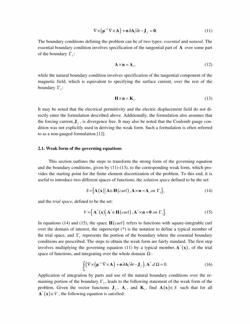
The boundary conditions defining the problem can be of two types: essential and natural. The
essential boundary condition involves specification of the tangential part of A over some part
of the boundary 1Γ :
,t× =A n A (12)
while the natural boundary condition involves specification of the tangential component of the
magnetic field, which is equivalent to specifying the surface current, over the rest of the
boundary 2Γ :
.t× =H n K (13)
It may be noted that the electrical permittivity and the electric displacement field do not di-
rectly enter the formulation described above. Additionally, the formulation also assumes that
the forcing current, fJ , is divergence free. It may also be noted that the Coulomb gauge con-
dition was not explicitly used in deriving the weak form. Such a formulation is often referred
to as a non-gauged formulation [12].
2.1. Weak form of the governing equations
This section outlines the steps to transform the strong form of the governing equation
and the boundary conditions, given by (11)-(13), to the corresponding weak form, which pro-
vides the starting point for the finite element discretization of the problem. To this end, it is
useful to introduce two different spaces of functions; the solution space defined to be the set:
( ) ( ) 1, ,tS curl on= ∈ × = ΓΑ x A H A n A (14)
and the trial space, defined to be the set:
( ) ( ) * * *
1, .V curl on= ∈ × = ΓΑ x A H A n 0 (15)
In equations (14) and (15), the space ( )curlH refers to functions with square-integrable curl
over the domain of interest, the superscript (*) is the notation to define a typical member of
the trial space, and 1Γ represents the portion of the boundary where the essential boundary
conditions are prescribed. The steps to obtain the weak form are fairly standard. The first step
involves multiplying the governing equation (11) by a typical member, ( )*A x , of the trial
space of functions, and integrating over the whole domain Ω :
( )( )1 *. 0.ft d−
Ω
∇ × ∇ × + ∂ ∂ − Ω =∫ µ A σ A J A (16)
Application of integration by parts and use of the natural boundary conditions over the re-
maining portion of the boundary, 2Γ , leads to the following statement of the weak form of the
problem. Given the vector functions fJ , tA , and tK , find ( ) S∈A x such that for all
( )*V∈A x , the following equation is satisfied:

( ) ( )2
1 * * * *. . . . .f td t d d dS−
Ω Ω Ω Γ
∇ × ∇ × Ω + ∂ ∂ Ω = Ω +∫ ∫ ∫ ∫µ A A σ A A J A K A (17)
Equation (17) provides the starting point of a finite element based approximation, and a solu-
tion to (17) is said to satisfy the system (11)-(13) in a weak sense.
2.2. Finite element discretization of the weak form
The weak form is solved by discretizing the domain into a set of finite elements, where
the solution within each finite element is assumed to be known in terms of shape functions,
that belong to the solution space, S , and degrees of freedom or coefficients that scale the
shape functions. It is well known [4, 7, 14] that the standard node-based interpolation, that is
commonly used is structural mechanics finite element formulations, has serious limitations
when it comes to solving electromagnetic problems. Interpolation based on so called edge-
element formulations with vector shape functions is more appropriate and works better for
electromagnetic problems. Thus, within each element the magnetic vector potential, A , is
interpolated as:
( ) ( ) ,a aA=∑A x N x (18)
where ( )aS∈N x represents the a -th vector shape function for the element, and aA
represents the corresponding unknown degree of freedom, and the sum is carried out over the
total number of degrees of freedom in an element. The reader is referred to [10, and refer-
ences therein] for a detailed presentation of the vector shape function framework. For the pur-
pose of this paper it suffices to note that the vector shape functions are associated with the
element edges instead of the element nodes, and, for the lowest order elements, the degree of
freedom corresponding to a given edge represents the tangential component of A along the
edge, which is constant on that edge. The form of the interpolation given by equation (18),
and the interpretation of the shape functions and degrees of freedom discussed above, ensures
that A is tangentially continuous across inter-element boundaries. The normal component is
not continuous across element boundaries. The above continuity properties of the interpola-
tion are consistent with the theoretical continuity requirements [9, 13] on the electromagnetic
fields across boundaries between dissimilar materials.
2.3. Time-harmonic solutions
Applications such as induction heating are often driven by an alternating or time-
harmonic current. In this section the weak form developed above for the general problem is
specialized to time-harmonic problems. The corresponding development for transient prob-
lems requires a time-integration scheme, but is otherwise straightforward, and is not discussed
in this paper. It may be noted, however, that the Abaqus electromagnetic capabilities support
transient low-frequency electromagnetic as well as magnetostatic procedures. The forcing
(volume or surface) current density, assuming time-harmonic behavior, may be assumed to be
of the form (shown below only for the volume current density):

( ) ( )e ,o i t
f f
ω=J x J x (19)
where
( ) ( ) ( )o o o
f f R f Ii= +J x J x J x (20)
represents the amplitude of the time-harmonic applied volume current density with real (in-
phase) and imaginary (out-of-phase) components o
f RJ and o
f IJ , respectively, ω represents
the frequency of excitation, and 1i = − . After the transient effects upon the initial applica-
tion of the current load die out, the long-term solution may also be assumed to be of the same
time-harmonic form as the excitation, i.e.:
( ) ( )e ,o i tω=A x A x (21)
where ( )oA x represents the amplitude of the solution ( )A x
, and may be expressed as:
( ) ( ) ( ) ,o o o
R Ii= +A x A x A x (22)
in terms of its real (in-phase) and imaginary (out-of-phase) components. Substitution of (19)
through (22) into the weak form leads to:
( ) ( )2
1 * * * *. . . . ,o o o o o o o o
f td i d d dSω−
Ω Ω Ω Γ
∇ × ∇ × Ω + Ω = Ω +∫ ∫ ∫ ∫µ A A σA A J A K A (23)
which must be solved for ( )oA x .
In the rest of this paper all material properties are assumed to be isotropic and piecewise
constants (i.e., µ=µ I and σ=σ I , respectively, where µ and σ are scalar piecewise con-
stants that represent the isotropic values of the magnetic permeability and the electrical con-
ductivity, respectively, and I represents the second-order identity tensor), such that the
second-order tensor quantities representing the magnetic permeability and the electrical con-
ductivity in equation (23) can be replaced by the corresponding scalar quantities. The Abaqus
implementation does not have this limitation, and the materials properties can be functions of
the spatial coordinates. With the above simplifications, the final system of equations may be
written in matrix form as:
,oa oa oa
R I f Rσω+ =KA CA J (24)
.oa oa oa
R I f Iσ ω− + =CA KA J (25)
In the equations above, the “stiffness” matrix or the so-called curl-curl operator, K , is de-
rived from the first term in equation (23), while the “damping” matrix, σ C , is derived from
the second term in equation (23). The quantities oa
f RJ and oa
f IJ (the superscript a is an index
for the degree of freedom – consistent with equation (18)) represent the consistent current
loads at the edges, and are derived from the real and imaginary components of the applied
volume current density vector (equations (19) and (20)), making use of the right hand side of
equation (23). Finally the quantities oa
RA and oa
IA represent the real and imaginary compo-

nents, respectively, of the edge degrees of freedom. These quantities are the unknowns in the
above system of algebraic equations.
As an aside, it may be noted that equation (23) implies that in conductor regions (where
there is an induced eddy current density, eJ , but the forcing current density, fJ , is zero) the
divergence-free condition on both A and eJ is satisfied in a weak sense. However, the Cou-
lomb gauge condition (i.e., the divergence-free condition on A ) is not enforced in any man-
ner in the non-conductor regions of the domain.
2.4. Remarks on the curl-curl operator
For the discussion in this section it is assumed that the boundary conditions are homo-
geneous and of the essential type everywhere on the boundary. In this case it is easy to verify
that the curl-curl operator, K , derived from the first term of equation (23), is nonnegative (or
positive indefinite). In fact, ( ),KA A [here ( ). , . is the notation for the standard inner product
that is defined as the integral over the domain of the product of the two functions within the
bracket] is zero for ϕ= ∇A , where ( )ϕ x is any scalar function that satisfies the homogene-
ous condition × =A n 0 everywhere on the boundary. The above implies that the curl-curl
operator is strongly singular with a null space that contains all functions of the form ϕ∇ , and
that a system of linear equations involving only the curl-curl operator on the left hand side
may not be well-posed (in the sense of producing a solution) unless the right hand side is also
orthogonal to the aforementioned null-space.
The presence of the damping matrix serves to somewhat mitigate the effects of the sin-
gularity. However, in a typical eddy current analysis it is very common that large portions of
the model consist of electrically nonconductive regions, such as air and/or a vacuum. In such
cases it is well known that the associated system matrix can be very ill-conditioned; i.e., it can
have many singularities [2]. Different methods have been proposed in the literature over the
years to address the above issue. These methods are typically based on either introducing a
tree-gauging [14] technique to solve the system of equations, or adding an artificial
conductivity to the non-conducting regions, or iterative solvers [3, 8, and references therein]
that make use of (wherever possible) the analytically determined null-space of the curl-curl
operator in the context of multigrid formulations.
Abaqus uses a special iterative solution technique to prevent the ill-conditioned matrix
from negatively impacting the computed electric and magnetic fields. The default
implementation works well for many problems. However, there can be situations in which the
default numerical scheme fails to converge or results in a noisy solution. For such cases
Abaqus has built-in stabilization mechanisms that employs a “small” amount of artificial
electrical conductivity in the nonconductive parts of the domain. This approach helps
regularize the problem and allows Abaqus to converge to the correct solution. The artificial
electrical conductivity is chosen such that the electromagnetic waves propagating through
these regions undergo little modification and, in particular, do not experience the sharp
exponential decay that is typical when such fields impinge upon a real conductor. When the
user controls the stabilization directly by explicitly specifying the electrical conductivity in

nonconducting regions, it is recommended that the artificial conductivity be set to be about
five to eight orders of magnitude less than that of any of the conductors in the model.
3. EXAMPLES
This section presents four brief examples of eddy current problems that make use of the
newly developed capabilities in Abaqus. All the problems are discussed in detail in [6], and
the reader is referred to this reference for additional details beyond those presented here.
Three of the examples are adapted from a standard suite of problems designed for Testing
Electromagnetic Analysis Methods (henceforth abbreviated TEAM), while the fourth example
presents a study of a transverse flux induction heating problem. Three of the examples
involve time-harmonic simulations, while one example corresponds to a transient simulation.
Figure 1: Geometry of an infinite conducting cylindrical shell immersed in a time-harmonic
uniform magnetic field.
3.1. TEAM 2 (Eddy current simulations of long cylindrical conductors in an oscillating
magnetic field)
The problem setup is shown in Figure 1. It depicts an infinite conducting cylindrical
shell immersed in a time-harmonic uniform magnetic flux density. The inner and outer radius
of the conducting cylindrical shell are a = 0.05715 m and b = 0.06985 m, respectively. Its
resistivity and relative magnetic permeability are assumed to be ( )1 σ = 3.94 x 10⁻⁸
Ω -m and
rµ = 1.0, respectively. The magnetic flux density is assumed to have a magnitude of oB = 0.1
a
b
σ, µr
θ
µ0
B0
z
y
x

T and is oscillating with a frequency of f = 60 Hz. The magnetic flux density is assumed to
be oriented in the y-direction. It is assumed that the medium in which the cylindrical shell is
immersed has properties similar to that of a vacuum. For these parameters, the skin depth of
the conductor is about ( )2 o rδ ωµ µ σ= = 12.9 mm, which is comparable to the shell
thickness of 12.9 mm.
The analytical solution to this problem is known and is provided in [6]. Figure 2 shows the
comparison of the amplitude of the y-component of the magnetic flux density computed using
Abaqus with that of the analytical solution. The labels `EMC3D8' and `EMC3D4' in the
legend correspond to the analyses performed with hex-shaped and tet-shaped finite elements,
respectively. The labels ‘Analytical Truncated’ and ‘Analytical True’ in the legend
correspond to the analytical solution computed by assuming that the essential.
Figure 2: Amplitude of the y-component of magnetic flux density.
boundary condition is applied on an outer cylindrical boundary surface at a finite distance and
at infinity, respectively. The figure clearly indicates that the analysis results compare very
well with the analytical results.
3.2. TEAM 4 (Eddy current simulation of a conducting brick in a decaying magnetic
field)
The problem domain consists of a rectangular brick with a centrally-located rectangular
through hole, which is placed in a uniform magnetic field that is decaying in time. The objec-
tive is to compute the circulating eddy currents induced in the brick and the ensuing Joule
heat that is dissipated. The problem setup is shown in Figure 3. The dimensions of the brick
are: a = 0.1524 m, b = 0.1016 m, and c = 0.0508 m. The brick is assumed to be made of an
aluminum alloy with a resistivity of ( )1 / σ = 3.94 x 10⁻⁸
Ω -m and a relative magnetic per-
meability of rµ = 1.0. The dimensions of the hole are assumed to be l = 0.0889 m and w =
x in meters (y = 0, z = 0)0.00 0.10 0.20 0.30 0.40 0.50
Am
plit
ud
e o
f B
y in
Te
sla
0.05
0.10
0.15
EMC3D8
EMC3D4
Analytical Truncated
Analytical True

0.0381 m. The orientation of the magnetic flux density is assumed to parallel to the direction
of penetration of the hole and is assumed to be decaying as ( )expo
B B t τ= − with oB = 0.1 T
and τ = 0.0119 s. The medium surrounding the brick is assumed to have properties similar to
that of vacuum.
Figure 4 is shows the magnetic flux density computed using Abaqus for a transient elec-
tromagnetic analysis that is performed over a period of 20 ms. The magnetic flux density is
plotted along the thickness direction of the brick starting from the center of the hole. The dif-
ferent curves correspond to the values of the magnetic flux density at different instants of time
(as indicated in the legend). The horizontal axis must be multiplied by 6.35 to get the true
distance (in mm) along the thickness direction, and the vertical axis should be multiplied by
0.01 to get the flux density in Tesla. The axes are scaled in this manner to facilitate the com-
parison of the Abaqus results against the results presented in [11]. The plot indicates that far
away from the conducting brick, the magnetic flux density is the same as that of the external
Figure 3: Geometry of a brick with a through hole placed in a declaying magnetic field.
field which is decaying in time. However, at the center of the brick, the magnetic flux density
is larger due to the eddy currents that are induced in the brick, which will try to compensate
for the magnetic flux density that is reducing in time. The results compare very well to those
published in [11].
c
ab
w
Bz=B
0 exp (−t/τ)
l

Figure 4: Time-variation of the variation of magnetic flux density in the thickness direction.
3.3. TEAM 6 (Eddy current simulations for spherical conductors in an oscillating
magnetic field)
The problem domain consists of a conducting spherical shell immersed in a time-harmonic
uniform magnetic field. The objective is to compute the eddy currents induced in the spherical
shell by the magnetic field that is varying in time. Lorentz force and Joule heating in the
conductor are also of interest. The problem setup is shown in Figure 5. For visual clarity, the
figure depicts the spherical shell with a section of it removed. The inner and outer radius of
the shell are a = 0.05 m and b = 0.055 m. Its conductivity and relative magnetic permeability
are assumed to be σ = 5 x 10⁸ S/m and rµ = 1.0. The magnetic flux density is assumed to
have a magnitude of oB = 1.0 T and is oscillating with a frequency of f = 50 Hz. Without loss
of generality, it can be assumed that the magnetic field is oriented along the z-direction. The
medium in which the spherical shell is immersed is assumed to have properties similar to that
of a vacuum. For these parameters, the skin depth of the conductor is about
( )2 o rδ ωµ µ σ= = 3.18 mm, which is smaller than the shell thickness of 5 mm.
The analytical solution to this problem is known and is provided in [6]. Figure 6 shows
the comparison of the amplitude of the z-component of the magnetic flux density computed
using Abaqus, with that of the analytical solution. The labels ‘EMC3D8’ and ‘EMC3D4’ in
the legend correspond to analyses performed using hex-shaped and tet-shaped finite elements,
respectively. The labels ‘Analytical Truncated’ and ‘Analytical True’ in the legend
correspond to the analytical solution computed by assuming that the essential boundary
condition is applied on an outer spherical boundary surface at a finite distance and at infinity,
respectively. The figure clearly indicates that the analysis results compare very well with the
analytical solution.
Distance along z−axis (x 6.35 mm) (x = y = 0)0. 5. 10. 15. 20.
Ma
gn
etic f
lux d
en
sity B
z (
x 0
.01
T)
0.0
2.0
4.0
6.0
8.0
10.0
4 ms8 ms12 ms16 ms20 ms4 ms8 ms12 ms16 ms20 ms

Figure 5: Geometry of a spherical shell immersed in a time-harmonic uniform magnetic field.
Figure 6: Amplitude of the y-component of magnetic flux density.
a
b
µ0
B0
z
y
x
σ, µr
ϕθ
x in meters (y = 0, z = 0)0.00 0.05 0.10 0.15 0.20 0.25 0.30
Re
al p
art
of
Bz in
Te
sla
0.0
0.4
0.8
1.2
EMC3D8
EMC3D4
Analytical Truncated
Analytical True

3.4. Transverse flux induction heating of a thin metallic sheet
Figure 7: Typical setup for transverse flux induction heating.
Transverse flux induction heating
tive when thin strips of metals need to be heated uniformly
the strip is usually of the same order of magnitude as the s
tion of the electromagnetic fields into the metallic medium.
can be very effective in understanding the design parameters that would lead to uniformity of
temperature distribution in the work
The Abaqus simulation consists of two separate analyses: an electromagnetic analysis to
compute the induced eddy current density and Joule heating in the conducting workpiece, and
a transient heat transfer analysis that uses the
tromagnetic analysis to compute the temperature
The typical setup of a TFIH apparatus is shown in Figure 7. The
current at a known frequency. The time
which is accentuated and focused utilizing magnetic cores
upon the aluminum sheet (workpiece)
in the workpiece, and Joule heating arises when the energy dissipated by the eddy currents
flowing through the workpiece is converted into thermal energy.
moves with a translational velocity (in the direction of its length) to ensure uniform heating.
The results presented here do not account for
electromagnetic analysis are presented below.
Figures 8, 9, and 10 shows plots of the electric fie
Joule heating distribution in the workpiece, as computed by a time
simulation in Abaqus. The parameters used for the modeling correspond to a typical TFIH
setup; the results are likewise quite gen
The distribution of the Joule heating intensity shows some nonuniformity along the edges at
locations that are below the ‘arms’ of the magnetic core
any magnetic shields along the edges of the metallic strip
3.4. Transverse flux induction heating of a thin metallic sheet
Figure 7: Typical setup for transverse flux induction heating.
Transverse flux induction heating (henceforth abbreviated TFIH) is important and effe
tive when thin strips of metals need to be heated uniformly [1]. In such cases, the thickness of
the strip is usually of the same order of magnitude as the skin-depth or the depth of penetr
tion of the electromagnetic fields into the metallic medium. Simulations of the TFIH process
can be very effective in understanding the design parameters that would lead to uniformity of
temperature distribution in the workpiece, as well as overall efficiency of the heating sys
simulation consists of two separate analyses: an electromagnetic analysis to
compute the induced eddy current density and Joule heating in the conducting workpiece, and
transfer analysis that uses the Joule heating intensity computed by the ele
tromagnetic analysis to compute the temperature distribution in the workpiece.
The typical setup of a TFIH apparatus is shown in Figure 7. The coils carry alternating
a known frequency. The time-varying current sets up a time-varying magnetic field,
which is accentuated and focused utilizing magnetic cores, and which impinge
(workpiece). The time-varying magnetic field induces eddy currents
Joule heating arises when the energy dissipated by the eddy currents
flowing through the workpiece is converted into thermal energy. The workpiece typically
onal velocity (in the direction of its length) to ensure uniform heating.
do not account for the motion. Only the results for the
electromagnetic analysis are presented below.
Figures 8, 9, and 10 shows plots of the electric field, magnetic flux density, and the
Joule heating distribution in the workpiece, as computed by a time-harmonic electromagnetic
The parameters used for the modeling correspond to a typical TFIH
setup; the results are likewise quite general and do not correspond to a specific TFIH problem.
The distribution of the Joule heating intensity shows some nonuniformity along the edges at
locations that are below the ‘arms’ of the magnetic core, as expected in a TFIH device without
any magnetic shields along the edges of the metallic strip.
is important and effec-
In such cases, the thickness of
depth or the depth of penetra-
Simulations of the TFIH process
can be very effective in understanding the design parameters that would lead to uniformity of
piece, as well as overall efficiency of the heating system.
simulation consists of two separate analyses: an electromagnetic analysis to
compute the induced eddy current density and Joule heating in the conducting workpiece, and
puted by the elec-
carry alternating
magnetic field,
impinges transversely
varying magnetic field induces eddy currents
Joule heating arises when the energy dissipated by the eddy currents
The workpiece typically
onal velocity (in the direction of its length) to ensure uniform heating.
Only the results for the
ld, magnetic flux density, and the
harmonic electromagnetic
The parameters used for the modeling correspond to a typical TFIH
eral and do not correspond to a specific TFIH problem.
The distribution of the Joule heating intensity shows some nonuniformity along the edges at
expected in a TFIH device without

Figure 8: Electric field during TFIH.
Figure 9: Magnetic flux density during TFIH.
Figure 10: Distribution of Joule heating in the workpiece.
4. CONCLUDING REMARKS
This paper presents some
commercial finite element software package,
broad range of electromagnetic problems. In particular, the new capabilities provide solutions
to Maxwell’s equations under the standard low frequency assumption
neering problems that are addressed are broadly known as eddy current problems, and include
induction heating as an important application.
Figure 8: Electric field during TFIH.
Figure 9: Magnetic flux density during TFIH.
Figure 10: Distribution of Joule heating in the workpiece.
4. CONCLUDING REMARKS
This paper presents some of the recent advances in the multiphysics portfolio of the
cial finite element software package, Abaqus, which are aimed at solving
netic problems. In particular, the new capabilities provide solutions
ons under the standard low frequency assumption. The classes of eng
dressed are broadly known as eddy current problems, and include
portant application. Although most of the presentation in this paper
recent advances in the multiphysics portfolio of the
are aimed at solving a fairly
netic problems. In particular, the new capabilities provide solutions
. The classes of engi-
dressed are broadly known as eddy current problems, and include
Although most of the presentation in this paper

focuses on time-harmonic solutions, the capabilities available in Abaqus are general enough
to solve transient electromagnetic and magnetostatic problems. Although the discussion in the
present paper was limited to linear magnetic behavior, complexities related to nonlinear but
monotonic magnetic constitutive response (characterized by a nonlinear B-H curve) can also
be accounted for in transient and magnetostatic procedures.
The formulation of the problems was described in some detail starting with a discussion
of Maxwell’s equations. This was followed by a discussion of a non-gauged solution ap-
proach based on the magnetic vector potential. The weak form and the final matrix form of
the discrete problem were described in some details in the context of a time-harmonic solution
procedure. Complications arising due to the presence of a significantly large null-space of the
curl-curl operator, and methods to mitigate them, were also discussed.
A number of example problems were presented. In all but one problem, the Abaqus si-
mulation results were compared to analytical solutions and were found to be in excellent
agreement. The final example discussed a generic setup of a transverse flux induction heating
(TFIH) problem.
Abaqus provides a strong multiphysics portfolio, and the new electromagnetic capabili-
ties augment this portfolio allowing users to carry out more realistic simulations in an inte-
grated manner with all the other capabilities of Abaqus, mainly in the areas of structural me-
chanics and heat transfer.
Acknowledgements
The authors would like to thank various members of the Mechanics, Materials and Electro-
magnetics, and Solver groups of the R&D organization of Dassault Syetemes Simulia Corp.
for their help during various stages of this work. Valuable discussion with members of the
CTO office is also gratefully acknowledged.
3. REFERENCES
[1] Barglik, J., “Induction Heating of Thin Strips in Transverse Flux Magnetic Field”. Ad-
vances in Induction and Microwave Heating of Mineral and Organic Materials, 207-232,
InTech, 2011.
[2] Bíró, O., “Edge Element Formulation of Eddy Current Problems”. Comp. Methods Appl.
Mech. & Engg., 169, 391-405, 1999.
[3] Bochev, P. B., Hu, J. J., Robinson, A. C., Tuminaro, R. S., “Towards Robust 3-D Z-Pinch
Simulations: Discretization and Fast Solvers For Magnetic Diffusion In Heterogeneous
Conductors”. Electronics Transactions on Numerical Analysis, Kent State University, 15,
186-210, 2003.
[4] Bossavit, A., “Computational Electromagnetism”. Academic Press, Boston, 1998.

[5] Dassault Systemes Simulia Corp., “Abaqus Analysis User’s Manual”. V6.12, 2012.
[6] Dassault Systemes Simulia Corp., “Abaqus Benchmarks Manual”. V6.12, 2012.
[7] Hiptmair, R., “From E To Edge Elements”. The Academician, 3 (No. 1), 23-31, 2003.
[8] Hiptmair, R., Xu, J. “Auxiliary Space Preconditioning for Edge Elements”. IEEE Trans.
Magnetics, 44 (No. 6), 938-941, 2006.
[9] Jackson, J. D., “Classical Electrodynamics”. John Wiley & Sons, Inc., 1999.
[10] Jin, J., “The Finite Element Method in Electromagnetics”. John Wiley & Sons, Inc.,
2002.
[11] Kameari, A. “Results for Benchmark Calculations of Problem 4 (the FELIX brick)”.
COMPEL, 7, 65-80, 1988.
[12] Ren, Z., “Influence of the R.H.S. on the Convergence Behavior of the Curl-Curl Equa-
tion”. IEEE Trans. Magnetics., 32 (No. 3), 655-658, 1996.
[13] Stratton, J. A., “Electromagnetic Theory”. McGraw Hill Book Company, 1941.
[14] Webb, J. P., “Edge Elements and What They can do for you”. IEEE Trans. Magnetics.,
29 (No. 2), 1460-1465, 1993.