Recent advances on nonlinear Reduced Order Modelling for stability andbifurcations problems in incompressible fluid dynamics

Giuseppe Pitton, Gianluigi Rozza∗

SISSA, International School for Advanced Studies, Mathematics Area, mathLab, via Bonomea 265, 34136, Trieste, Italy

Abstract

In this paper we propose a Reduced Basis framework for the computation of bifurcation and stabilityproblems arising from nonlinear partial differential equations. The proposed method aims at reducing thecomplexity and the computational time required for the construction of bifurcation and stability diagrams.The method is quite general since it can in principle be specialized to a wide class of nonlinear problems,but in this paper we focus on an application in incompressible Fluid Dynamics at low Reynolds numbers.The validation with a benchmark cavity flow problem is satisfactory.

Keywords: Reduced Basis Method, Proper Orthogonal Decomposition, Steady Bifurcation, HopfBifurcation, Navier Stokes, Flow Stability, Spectral Element Method

1. Introduction

The study of stability and bifurcation of nonlinear systems is an established research field, of greatimportance both from the applied mathematics and engineering perspective.

The aim of Bifurcation Theory is the computation of branches of non-unique solutions for nonlinearproblems [1], and the detection of the intersection points between the solution branches, called bifurcationpoints, as a function of some physical or geometrical control parameters.

Some typical control parameters are the geometrical aspect factors, or relevant adimensional quantities(such as the Reynolds number, or the Grashof number), or the boundary conditions, or forcing terms.

Usually the results of a stability analysis are represented in a diagram where the stability region ofeach branch of solutions is depicted as a function of the control parameters. Bifurcation diagrams show aqualitative or quantitative (pointwise or integral) aspect of a solution as a function of the control parameters,allowing to understand the structure and the physical features of the solution set. See for example [2] for aclassical introduction to stability problems in Fluid Mechanics.

For instance, Bifurcation Theory is of evident practical importance in the analysis of stability problemsin Elasticity, where it is well known that for many structures there exists a critical load which if exceededwill produce a catastrophic collapse (a classic reference on this subject is [3], a more mathematically orientedone is [4]).

Common applications of Bifurcation Theory in Fluid Mechanics include a wide range of industrial prob-lems such as tribology, microfluid dynamics, biomedical industry, biomedicine (blood flows), and many more.In particular, the field of hydrodynamic stability focuses on the classification of the nature of flows as somecontrol parameters are varied [2]. Specifically, the purpose of a stability investigation is, given a well-definedinitial or boundary value problem, to classify the asymptotic solutions as stable, or time periodic, or evenchaotic in time.

∗Corresponding authorEmail addresses: gpitton@sissa.it (Giuseppe Pitton), grozza@sissa.it (Gianluigi Rozza)

Preprint submitted to Elsevier February 24, 2015

The construction of stability maps and bifurcation diagrams is a delicate and very expensive task,requiring an important computational effort and prohibitive if the number and range of parameters is large.This is particularly true for three and higher dimensional simulations.

Recent developments of Reduced Order Modelling (ROM) techniques have focused on the reduction ofcomputational time for a wide range of differential problems, while mantaining a prescribed tolerance onerror bounds [5]. It is therefore of great interest to further investigate how such methods can be applied tostability problems in Fluid Dynamics and Elasticity in order to reduce the computational power required.

The literature has already shown the effectiveness of Proper Orthogonal Decomposition (POD) bothfor analysis of principal modes [6] and for the reduction of computational power required by transientsimulations. For instance, Terragni and Vega [7] showed how a POD approach could save a considerableamount of computing time for the analysis of bifurcations in some nonlinear dissipative systems. In a recentpaper Herrero, Maday and Pla [8] have shown that both POD and the Reduced Basis Method (RBM)can reconstruct the behaviour of velocity and temperature field for a two-dimensional natural convection(Boussinesq) problem with large reduction of the computational power with respect to classical techniques.In particular, stable and unstable solutions are correctly identified, and a surrogate error estimate is alwaysmantained below a prescribed tolerance. A recent remarkable work by Yano et al. [9] introduced a RBMethod for the stability of flows under perturbations in the forcing term or in the boundary conditions,based on a space-time framework that allows for particularly sharp error estimates.

Summarizing, given the relatively fast decay of energy spectrum for flows at sufficiently low Reynoldsnumbers, a Reduced Order Modelling technique could be expected to be an efficient tool for flow stabilityanalysis. Reduced Basis (RB) techniques [10] historically have been proven effective for the study of elasticstability of plates [11], but their application in more complex parametrized stability problems such as inFluid Mechanics is an open and quite relevant research field.

In this paper, we propose the application of Reduced Order Modeling (ROM) techniques to reducethe quite demanding computing costs for bifurcation and stability analysis of flows. We will consider abenchmark problem well known in the literature, namely a buoyancy-driven flow in a rectangular cavity [12].

The focus of this work is devoted on several improvements with respect to the state of the art for theseproblems, approached with ROM: in particular we mention approximation stability, sampling, and reducedeigenproblems for stability analysis. Our exposition presents the topic from the different viewpoints ofNonlinear Mathematical Analysis, Applied Mathematics and Numerical Analysis, trying to underline thedifferent aspects of the problem under consideration.

The structure of the paper is the following. In section 2 we present the class of abstract problems that willbe considered and we briefly recall some important results on Nonlinear Analysis and Bifurcation Theory.Section 3 is devoted to the presentation of a general ROM technique and particular attention is devotedto the approximation of bifurcation problems. In section 4 the mathematical setting for the approximationof incompressible Fluid Dynamics equation is recalled, and the high-order method used is presented. Insection 5 the ROM technique previously developed is specialized to the Navier-Stokes case and finally somenumerical results are show and discussed in section 6.

2. Abstract setting

We start our discussion of reduction strategies for bifurcation and stability problems recalling somebasic elements of Nonlinear Analysis that will prove to be useful in the applications. Despite being arelatively recent field, there are at least two main frameworks of Nonlinear Analysis of striking effectiveness, atopological one and a variational one. Roughly, the motivation behind these two approaches are respectively:

• consider at the problem as a functional equation between Banach spaces, and study it in a purelyabstract setting [1] (e.g. using Implicit Function Theorem, Degree Theory, etc.);

• when possible, exploit the variational structure of the problem, and find solutions as stationary pointsof some “energy” functional [13].

2

We will focus on the first approach, since the latter is limited to equations derived from a variationalprinciple, most notably semilinear elliptic equations. Furthermore, most of the existing results of NumericalAnalysis for nonlinear problems are cast in such setting. This setting is quite abstract, in fact it encompassesa large class of maps between functional spaces, such as differential and integral equations. As a result theresults obtained are very general although we will mainly be concerned on differential problems.

We consider nonlinear problems depending on a parameter µ ∈ D ⊂ Rp in the form: find u ∈ X suchthat:

〈F (µ, u), v〉 = 0 ∀v ∈ Y, (1)

where F : D×X → Y ′ is a map, X and Y are Banach spaces and the angled parenthesis denote the dualitypairing between Y and its dual space Y ′. The family of parameter-dependent solutions u(µ)µ∈D formsa subset of X, and for some parameter values there may be some qualitative changes in the structure ofthe solutions. For instance, there may be a loss of uniqueness of the solution, usually followed by a changein the stability properties under infinitesimal or finite perturbations, or the transition from steady state totime dependent solutions, just to mention a few possibilities.

Rigorously, we say that (µ∗, u∗) is a bifurcation point for (1) if there exist at least two sequences(µ1m, u

1m) ⊂ D ×X, (µ2

n, u2n) ⊂ D ×X such that:

i) (µ1m, u

1m) 6= (µ2

n, u2n) ∀m,n ∈ N;

ii) 〈F (µim, uim), v〉 = 0 ∀v ∈ Y, for i = 1, 2;

iii) (µ1m, u

1m)→ (µ∗, u∗) and (µ2

n, u2n)→ (µ∗, u∗) ∀m,n ∈ N.

We define the (Frechet) differential of F with respect to the variable u, defined if exists a linear operatorDuF (µ, u) ∈ L (X,Y ′) such that:

lim‖w‖X→0

‖F (u+ w)− F (u)−DuF (µ, u)[w]‖Y ′

‖w‖X∀w ∈ X. (2)

With L (X,Y ) we denote the set of all linear continuous operators from X to Y , and we denote withDuF (µ, u)[v] ∈ Y ′ the action on v ∈ X of the differential of F with respect to the variable u evaluated atthe point (µ, u). Many important results in Nonlinear Analysis depend on the existence of partial derivativesof the operator F .

The simplest case is when the partial derivative is an isomorphism fromX to Y ′, and we writeDuF (µ, u) ∈Iso(X,Y ′). In this case we say that (µ∗, u∗) is a regular solution (or a nonsingular solution) of (1), and itsexistence and uniqueness are ensured locally by the Implicit Function Theorem (IFT) [1]. The fact thatthe map F is invertible with invertible differential means practically that it is possible to express locallyu as a function of µ. This is possible only if the differential DuF (µ∗, u∗) is invertible, since in this caseDuF (µ∗, u∗)−1 : Y ′ → X maps neighbourhoods into neighbourhoods.

In contrast, if (µ∗, u∗) is a bifurcation point of (1), then DuF (µ∗, u∗) is not invertible, and it is impossibleto express u as a function of µ directly. In particular, when DuF (µ∗, u∗) /∈ Iso(X,Y ′) two possibilities arise:

DµF (µ∗, u∗) /∈ R(DuF (µ∗, u∗)) limit point;

DµF (µ∗, u∗) ∈ R(DuF (µ∗, u∗)) bifurcation point;(3)

where DµF (µ∗, u∗) is the partial derivative of F with respect to the parameter µ. For both cases we supposealso that DuF (µ∗, u∗) has a closed range and satisfies:

dim ker(DuF (µ∗, u∗)) = dim(R(DuF (µ∗, u∗))⊥) (4)

where R(DuF (µ∗, u∗))⊥ is the orthogonal complement to R(DuF (µ∗, u∗)), such that Y ′ can be written asa direct sum:

Y ′ = R(DuF (µ∗, u∗))⊕ R(DuF (µ∗, u∗))⊥, (5)

3

and kerF = v ∈ X s.t. F (v) = 0 is the kernel of the operator F . We mentioned that the Implicit FunctionTheorem plays a fundamental role when studying the properties of the solution set of equation (1). Theform of the IFT that we consider here is the following: let F ∈ Ck(Λ × U, Y ′) with k ≥ 1, Λ ⊆ D, U ⊆ X,and suppose that (µ∗, u∗) ∈ Λ× U are such that

〈F (µ∗, u∗), v〉 = 0 ∀v ∈ Y DuF (µ∗, u∗) ∈ Iso(X,Y ′), (6)

that is, u∗ solves the problem (1) with the parameter µ∗ and the u partial derivative of F is invertible in aneighbourhood of (µ∗, u∗). In particular, there exist neighbourhoods Ξ ⊆ D of µ∗ and V ⊆ X of u∗ and amap γ ∈ Ck(Ξ , X) such that:

〈F (µ, γ(µ)), v〉 = 0 ∀v ∈ V,∀µ ∈ Ξ . (7)

In the next paragraphs, the Implicit Function Theorem will be frequently applied to parametrize solutionsets in a neighbourhood of a singular point and allow the following of solution branches.

2.1. Limit points

We consider limit points (µ∗, u∗) such that the differential DuF (µ∗, u∗) is compact and has a one-dimensional kernel, dim kerDuF (µ∗, u∗) = 1. Let ϕ0 ∈ X be a basis for the kernel of DuF (µ∗, u∗). Inthis case the differential map is not an isomorphism, and the Implicit Function Theorem cannot be applieddirectly to parametrize u with respect to µ. However, introducing a new parameter s ∈ [−ε, ε], the solutionset can be parametrized in a neighbourhood of the limit point:

µ(s) = µ∗ + ξ(s)

u(s) = u∗ + sϕ0 + γ(ξ(s), s)(8)

for a map ξ : [−ε, ε] → R. The existence of the map ξ is important both for building an approximationstrategy for the fold points and in the following of the solution branch in a neighbourhood of a fold point.

2.2. Bifurcation points

In the case of simple bifurcation points multiple branches of solution issue from a principal branch, hencethe study of the solutions set is a particularly delicate task. A classical tool in this case is provided by theLyapunov-Schmidt reduction, that allows to split the problem in an appropriate way such that the IFT canbe applied on some subsets of X and Y ′.

At a simple bifurcation point, we require that the differential DuF (µ∗, u∗) has a closed range and aone-dimensional kernel, dim kerDuF (µ∗, u∗) = 1 (although these hypotheses can be relaxed, see [14]). Letnow ϕ0 ∈ X be a basis for the kernel of DuF (µ∗, u∗) and ϕ∗0 ∈ Y ′ a basis for the topological complementof the range of DuF (µ∗, u∗). Next, let R(A) be the image of X under the operator A. We introduce aprojection on the range of the differential P : Y ′ → R(DuF (µ∗, u∗)) and its complementary projectionQ = I − P : Y ′ → (R(DuF (µ∗, u∗)))⊥:

Pw = 〈w,Rϕ∗0〉ϕ∗0 ∀w ∈ Y ′

Qw = w − 〈w,Rϕ∗0〉ϕ∗0 ∀w ∈ Y ′,(9)

where R : Y ′ → Y is the Riesz representation operator. The Lyapunov-Schmidt reduction consists in theprojection of equation (1) both on the range of DuF (µ∗, u∗) and on its complementary set. With the latterprojection we have the auxiliary equation

〈QF (µ, u), v〉 = 0 ∀v ∈ Y (10)

for which the Implicit Function Theorem can be applied to introduce two new parameters ξ, s and a mapγ : [−εξ, εξ]× [−εs, εs]→ R(DuF (µ∗, u∗)) such that we can express

µ = µ∗ + ξ

u = u∗ + ξϕ0 + γ(ξ, sϕ0).(11)

4

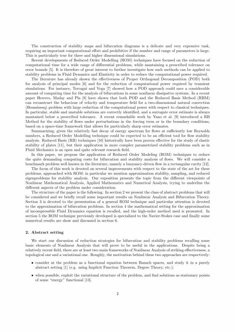
µu

(a) (b) (c)

••

•

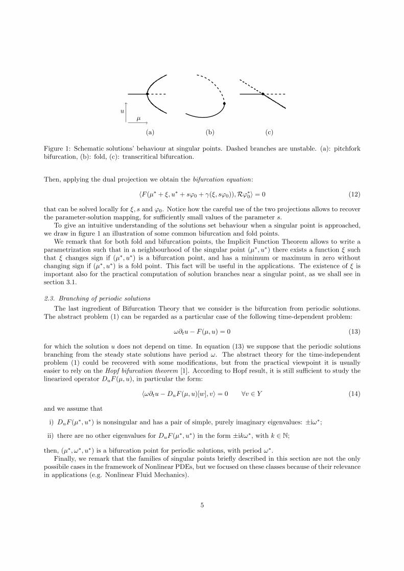
Figure 1: Schematic solutions’ behaviour at singular points. Dashed branches are unstable. (a): pitchforkbifurcation, (b): fold, (c): transcritical bifurcation.

Then, applying the dual projection we obtain the bifurcation equation:

〈F (µ∗ + ξ, u∗ + sϕ0 + γ(ξ, sϕ0)),Rϕ∗0〉 = 0 (12)

that can be solved locally for ξ, s and ϕ0. Notice how the careful use of the two projections allows to recoverthe parameter-solution mapping, for sufficiently small values of the parameter s.

To give an intuitive understanding of the solutions set behaviour when a singular point is approached,we draw in figure 1 an illustration of some common bifurcation and fold points.

We remark that for both fold and bifurcation points, the Implicit Function Theorem allows to write aparametrization such that in a neighbourhood of the singular point (µ∗, u∗) there exists a function ξ suchthat ξ changes sign if (µ∗, u∗) is a bifurcation point, and has a minimum or maximum in zero withoutchanging sign if (µ∗, u∗) is a fold point. This fact will be useful in the applications. The existence of ξ isimportant also for the practical computation of solution branches near a singular point, as we shall see insection 3.1.

2.3. Branching of periodic solutions

The last ingredient of Bifurcation Theory that we consider is the bifurcation from periodic solutions.The abstract problem (1) can be regarded as a particular case of the following time-dependent problem:

ω∂tu− F (µ, u) = 0 (13)

for which the solution u does not depend on time. In equation (13) we suppose that the periodic solutionsbranching from the steady state solutions have period ω. The abstract theory for the time-independentproblem (1) could be recovered with some modifications, but from the practical viewpoint it is usuallyeasier to rely on the Hopf bifurcation theorem [1]. According to Hopf result, it is still sufficient to study thelinearized operator DuF (µ, u), in particular the form:

〈ω∂tu−DuF (µ, u)[w], v〉 = 0 ∀v ∈ Y (14)

and we assume that

i) DuF (µ∗, u∗) is nonsingular and has a pair of simple, purely imaginary eigenvalues: ±iω∗;

ii) there are no other eigenvalues for DuF (µ∗, u∗) in the form ±ikω∗, with k ∈ N;

then, (µ∗, ω∗, u∗) is a bifurcation point for periodic solutions, with period ω∗.Finally, we remark that the families of singular points briefly described in this section are not the only

possibile cases in the framework of Nonlinear PDEs, but we focused on these classes because of their relevancein applications (e.g. Nonlinear Fluid Mechanics).

5

3. A discrete setting

Many of the results of Nonlinear Analysis exposed in section 2 apply in the finite-dimensional case,providing a rigorous foundation for the numerical approximation and strategies for the actual computation.A milestone in the numerical approximation of nonlinear problems is the theory developed by Brezzi, Rappazand Raviart [15, 16, 17] (BRR), to which we frequently refer in the rest of the section. A good introduction tothis theory is provided by [14]. In this section we rely on BRR theory for the case of Reduced Order Modellingthat has many analogies but also some specialities over the traditional Galerkin approximation methods,the most relevant being that the conventional general purpose bases with local support are replaced withproblem dependent bases endowed with global support. Referring for instance to [5] for a detailed overviewon the Reduced Order Methods of interest, we proceed recalling some basic facts about ROMs and PODthat will be useful in the following.

3.1. Truth approximation

The first step of a ROM (RB, POD, . . . ) is to extract information from a series of known solutionscharacterized by different values of the parameters. Usually these solutions need to be approximated througha computational method commonly called truth approximation in the community, which can be any classicaldiscretization method for PDEs (such as the Finite Element Method, Spectral Element Method, FiniteVolume Method, etc). We focus here on (Petrov-)Galerkin projection methods, that recover much of thesetting in the original problem (1). The approximated solution uN is obtained as projection of the fullsolution u on a finite dimensional subset XN of X (the superscript N denotes the dimension of XN ),and the test function space is replaced with a finite dimensional subset Y N of Y . As a result, the truthapproximation of problem (1) reads: find uN ∈ XN such that

〈F (µ, uN ), v〉 = 0 ∀v ∈ Y N . (15)

Throughout this work we assume that u 7→ F (λ, u) is a nonlinear map, and to obtain a linear algebraproblem from equation (15) we need to introduce a suitable approximation scheme. For instance, a possibleapproach consists in constructing a sequence of successive approximations uNk such that the k-th elementof the sequence solves a linearized problem. Let us write a decomposition of F into its linear and nonlinearparts, L and N :

F (µ, u) = µL(µ)u+N(µ, u), (16)

then two popular fixed point linearization strategies are as follows.

Picard iterations in this case we rewrite problem (15) as an approximation for a fixed point of F . Atiteration k + 1, solve for uNk+1:

〈L(µ)uNk+1 +N(µ, uNk ), v〉 = 0 ∀v ∈ Y N (17)

Banach-Caccioppoli theorem ensures that a fixed point exists and is unique provided that F is acontraction map on a sufficiently large ball B(u0) ⊂ X, i.e. there exists a constant l ∈ (0, 1) such that

‖F (µ, u)− F (µ,w)‖Y ′ ≤ l‖u− w‖X ∀u,w ∈ B(u0) (18)

and that uNk → uN in the norm of X.

Newton-Kantorovich iterations in this case also the first differential of F is exploited:〈F (µ, uNk ) +DuF (µ, uNk )[wNk+1], v〉 = 0 ∀v ∈ Y N

uNk+1 = uNk + wNk+1.(19)

Newton-Kantorovich iterations are convergent if a Lipshitz condition is satisfied on the differential ofF :

‖DuF (µ, u)[v]−DuF (µ, u)[w]‖Y ′ ≤ l‖v − w‖X ∀u, v, w ∈ S (20)

where S is an appropriate open convex subset of X.

6

We remark that convergence results are available [18] in both cases also when the operator F is beingapproximated by a sequence Fh ⊂ Iso(X,Y ′) such that consistency is preserved, Fh(µ, uNk ) → F (µ, uN ).This fact is of particular importance since often in Numerical Analysis the continuous operators are replacedwith discrete operators e.g. exact integrals are approximated by quadrature formulas.

After the linearization, it is possible to derive a linear algebra problem simply by expanding the approx-imate solution at k-th iteration: uNk =

∑Ni=1 u

Nk,iϕi where ϕi and ψj are basis sets respectively for XN

and Y N . Replacing the series expansion for uN , and choosing v = ψj , we have a linear algebra problem:

Akuk = bk, (21)

for each step k, whose terms have the form:

Ak,ij = 〈L(µ)ϕi +DuF (µ, uNk−1)[ϕi], ψj〉 uk,i = uNk,i, bk,i = 〈N(µ, uNk , ψi〉. (22)

System (21) can then be solved by the usual techniques (see for instance [19]). However, our discussion ofthe algebraic problem is only illustrative, and in the real practice much more complex discretization methodsare used. In particular, for medium and large sized problems it is mandatory to distribute the computationbetween many CPUs, for instance via a Domain Decomposition Method (see [20] or [21]).

The presence of multiple solutions for a given parameter value requires some care to ensure that thecomputed solutions belong to the same branch, as in some cases the computation could oscillate between twosolutions without converging. A popular method to deal with this problem is the continuation method [22].In its simplest version, it consists of two steps:

Step 1. predictor: starting from a known solution (µk, uk), compute a prediction (µk, uk) = (µk+∆µk, uk+∆uk) on the tangent space to (µk, uk) by solving for ∆uk the problem:

DµF (µk, uk)∆µk +DuF (µk, uk)∆uk = 0, (23)

where ∆µk is given (and sufficiently small);

Step 2. corrector: starting from the prediction (µk, uk), solve iteratively the original problem (1) imposingthe additional constraint that the solutions are orthogonal to the tangent space at (µk, uk):

DµF (µki , uki )∆µki +DuF (µki , u

ki )∆uki = −F (µki−1, u

ki−1)

(µk,∆µki )D + (uk,∆uki )X = 0

µki = µki−1 + ∆µki uki = uki−1 + ∆uki

(24)

with the starting condition that the sequence of approximant solutions issues from the predictorsolution:

µk0 = µk uk0 = uk. (25)

3.2. Sampling

The information needed for building a reduced order approximation is obtained by constructing a setof properly selected truth solutions uN (µi)Ni=1 ⊂ XN computed for a suitable sequence in the parameterspace µiNi=1 ⊂ D. There exist different methods1 for identifying a sequence µi ⊂ D, often based on a“worst case” criterion, which given an initial sequence µiki=1, aims at searching for the parameter µk+1

whose solution is the worst approximated one within the space spanned by the snapshots Sk = uN (µi)ki=1.Then, the new solution uN (µk+1) is added to the snapshots space Sk+1 = Sk∪uN (µk+1) and the algorithmis restarted until a suitable stopping criterion is satisfied.

Two of the most popular sampling methods based on a worst case strategy are the following.

1We refer the interested reader to [5] for a brief overview on the history of the Reduced Basis Method and a review of manysampling techniques.

7

Greedy Algorithm Very widely spread in the ROM community, we refer to [23] for a comprehensivereview and to [24, 25] for some relevant convergence estimates. Suppose that are given k − 1 lin-early independent snapshots Sk−1 = uNi ⊂ XN . Then the k-th snapshot is computed as solutioncharacterized by the parameter value µk ∈ D such that

µk = arg minµ∈D∥∥uN (µk)−ΠSku

N (µk)∥∥X, (26)

where ΠSk : XN → Sk is the projector on the space generated by Sk. Then uN (µk) is used to enrichthe snapshots space: Sk = Sk−1 ∪ uN (µk). To simplify the computation of the minimizer µk ofequation (26), usually two additional constraints are imposed:

• the parameter space D is replaced by a finite subspace Ξ ;

• the projection error ‖uN (µk)−ΠSkuN (µk)‖X is replaced by some parameter-dependent estimate

∆(µ) such thatc∆∆(µk) ≤

∥∥uN (µk)−ΠSkuN (µk)

∥∥X≤ C∆∆(µk) (27)

for c∆, C∆ > 0. This estimate is introduced to avoid computing the explicit solution uN (µk)and its projection for all µk ∈ Ξ . We discuss on section 3.9 a possible strategy for obtaing anexpression for ∆(µ).

These two approximations together give origin to the family of weak greedy algorithms.

It is easy to verify that the snapshot spaces produced by Greedy Algorithms are hierarchical spaces,that is S1 ⊂ S2 ⊂ · · · ⊂ Sk. This property has a great practical importance since it allows to enrichthe set of snapshots without throwing away the previously computed solutions, since the new one issimply added to the previous set.

Centroidal Voronoi Tessellation Centroidal Voronoi Tessellation (CVT) has been introduced by Duand Gunzburger [26] as sampling strategy for Reduced Order Modelling. We need to define threepreliminary concepts:

• a collection of subsets Viki=1 of D is called a tessellation of D if they are disjoint Vi ∩ Vj = ∅ if

i 6= j, and covering⋃ki=0 Vi = D;

• we endow the parameter space D with a distance function d induced by the norm of X betweenthe corresponding solutions:

d(µ1, µ2) = ‖uN (µ1)− uN (µ2)‖X . (28)

Then, given a set of points µi ⊂ D, we define the i-th Voronoi region Vi ⊂ D as:

Vi = ν ∈ D such that d(ν, µi) ≤ d(ν, µj)∀j 6= i, (29)

and µi ⊂ D are a set of given generating points.

• suppose that a density function % : D → R+ is given on the parameter space. Then we define themass centroid ξ ∈ D of a subset U of D as the barycenter of U , namely:

ξ = arg minν∈U

∫Ud(υ, ν)%(υ) dυ. (30)

Note that in general the generating points defining the Voronoi regions in (29) and the mass centroidsdefined in equation (30) do not coincide, but if this happens, the tessellation defined by the generatingpoints µi is named Centroidal Voronoi Tessellation (CVT).

A possible choice for the density function is the projection error as defined for the Greedy algorithm:

%(µ) =∥∥uN (µ)−ΠXNuN (µ)

∥∥X, (31)

8

where ΠXN : X → XN is the projection operator from X to its subspace XN (although in generalXN need not be a subspace of X; in this case supposing that both X and XN are imbedded in an“environment” set E, the projection ΠXN can be defined as the element in XN that minimizes thedistance in E from a given element in X). Then, if we define the “weight” of each Voronoi region Vias

Wi =

∫Vi

d(ν, ξi)%(ν) dν (32)

it can be shown that the CVT of dimension k of the parameter set is defined by the generating pointsµiki=1 that minimize the “total weight” functional:

F =

k∑i=1

Wi. (33)

In this sense the CVT is a best approximation sampling method, and is often combined with thePOD defined in section 3.3 to form the CVOD method [27], popular in the ROM community. To helpthe intuition on the meaning of the symbols entering in the integral (32), we refer to the sketch onfigure 3.2. Illustrative picture of some basic quantities entering in the definition of the CVT.

For computational purposes, some additional approximations are introduced, namely:

• as in the weak Greedy algorithm, D is replaced by Ξ and the projection error (31) by a suitableestimator ∆(µ);

• instead of computing all the generating points µk at each iteration, the first k points are kept fixedand only the k + 1-th generating point is computed as minimizer of the total weight functional (33);

• another possibility is to consider the Delaunay triangulation (dual of the Voronoi diagram) and take asnext point the barycenter of the triangle with the largest weight Wi. This technique has been introducedby Iollo et al. [28] for Delaunay samplings.

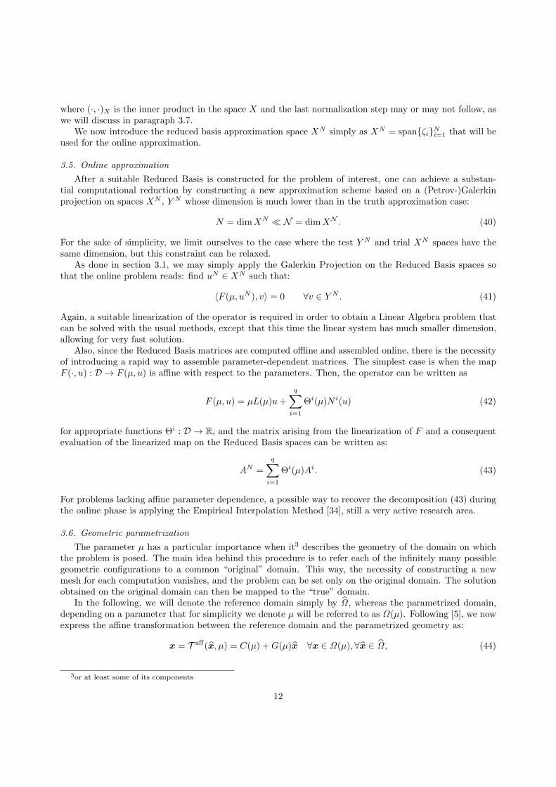
We remark that the last two strategies allow to obtain a hierarchical sampling.We sketch on figure 2 anexample step of CVT sampling procedure. The enhanced approximation properties of the RB space arevisualized by the reduction in density of the isolines of the weight function %.

In the description of Greedy and CVT sampling methods, we implied more or less explicitly that thesnapshot space contains only solutions of the original problem (1) for different parameter values, as done inthe classical Lagrangean interpolation theory. For this reason, ROMs based on such spaces are often calledLagrange ROM.

However, sampling methods are by no means restricted to Lagrange spaces, and can be applied to samplenot only the solutions manifold, but also the tangent bundle to the solutions manifold (originating HermiteROMs, [29]) or higher order derivative spaces (originating Taylor ROMs, [11]). Note that the solutionsmanifold and its tangent spaces are all embedded in the original space X, so there is no need to change thediscretization method for sampling Hermite or Taylor spaces.

Operatively, the tangent bundle is sampled by linearizing the original problem (1) and chosing amongall the possible small linear increments from the solution (µk, uk) the one closer to the solutions manifold.This is equivalent in finding Tuk ∈ X such that:

〈DuF (µk, uk)[Tuk], v〉 = −〈DµF (µk, uk), v〉 ∀v ∈ Y. (34)

For higher order sampling methods it is sufficient to impose that higher order Taylor expansions of theoriginal problem (1) are canceled out. For instance, a second order expansion would be in the form: findT 2uk ∈ X such that:

〈DuuF (µk, uk)[Tuk, T 2uk], v〉 = −〈2DuµF (µk, uk)[Tuk] +DµµF (µk, uk), v〉 ∀v ∈ Y, (35)

where DuuF (µ, u) ∈ L (X,X, Y ′) is a bilinear operator taking two elements of X to Y ′, or equivalently itcan be seen as a linear operator from X to the space of linear operators from X to Y ′, DuuF (µ, u)[w, ·] ∈L (X,Y ′). Similar considerations hold for the other second order differentials, DuµF (µ, u) and DµµF (µ, u).

9

Figure 2: One step of CVT sampling on a two parameters test case. The red dots show the sampled points,the isolines refer to the weight function %(ν). The black contours are the boundaries of each Voronoi region.On the left there is a representation of a sampling set in the parameters space consisting of 9 points. Onthe right the same set has been enriched by applying one step of the CVT algorithm. Note the new regionon the upper right part of the figure, and how the new sampled point has considerably stretched the regionconfined inside the isoline of minimum value.

We remark that Hermite spaces may be a particularly good choice when attempting a ROM in the caseof parametrized problems with multiple solutions. In fact, as exposed in section 3.1, a popular method toforce the computed solutions to lay on the same branch is the continuation method, that requires at eachiteration a solution of the tangent problem (34). Our claim is that Hermite sampling is an interesting choicein this case since it would simplify the computation of solutions branches during the online phase:

Step 1. in the predictor phase, impose the solution increment ∆uk of equation (23) to lay on the spacespanned by the tangent reduced basis set;

Step 2. during the correction phase, orthogonalize the reduced basis set with respect to the tangent basisset, in order to fulfill by construction the constraint on the orthogonality of the increments (24).

3.3. Proper Orthogonal Decomposition

When dealing with time-dependent problems, it is preferable not to add all the snapshots of a time-dependent run to the snapshots space Sk, otherwise the Reduced Basis Space will likely be too large andmany of the basis will be almost parallel, making the online projection phase an ill conditioned problem. Acommon technique is to extract the “most significant” modes of a time sequence using a RB approximationin combination with a Proper Orthogonal Decomposition [30]. There are many alternative ways to computethe POD modes of a sequence of snapshots uNi ⊆ XN . Here we focus on the method based on theeigenvalues of the correlation matrix [30]. The entries of the correlation matrix C ∈ RN×N are computed as

Cij = (uNi , uNj )V , (36)

then, if (λi, ψi) is a couple eigenvalue-eigenvector of C, each basis vector is computed as

ζi =

N∑k=1

ψi,kuNk (37)

10

where ψi,k denotes the k-th component of the i-th eigenvalue. The POD modes obtained are automaticallyorthogonal, but not normal in general. The eigenvalue λi associated to each POD mode is related to thefraction of energy stored in the corresponding mode.

A remarkable property of the space generated by the POD bases is that it minimizes the projectionerror in the norm of the space V of the snapshots used for the construction of the correlation matrix inequation (36):

XNPOD = spanζiNi=1 = arg minXN⊂X,dimX=N

N∑i=1

∥∥uNi −ΠXNuNi∥∥2

V. (38)

In this sense, the POD modes exhibit a best approximation property. It can be shown (see for instance [30])that the spaces spanned by the POD are hierarchical once the snapshots are fixed.

The sampling algorithms presented in section 3.2 are frequently combined with a POD for parametrizedtime-dependent problems. If a Greedy sampling algorithm is used to select the parameters, and the PODis used to recover the most relevant time snapshots, the sampling procedure is called POD-Greedy and werefer to [31] and [32] for details. To clarify the sampling process of time-dependent parametrized problems,we report in Algorithm 1 a possible implementation strategy of the POD-Greedy algorithm.

Algorithm 1 A POD-Greedy strategy for the sampling of parameter dependent evolution problems.

1: repeat

2: find µi+1 such that µi+1 = arg maxµ∈Σ∫ T

0‖uN (µi+1)−ΠSiu

N (µi+1)‖X dt3: compute a sequence of snapshots ui+1,krk=0 for the time dependent problem related to the param-

eter µi

4: compute the l POD modes of the sequence ϕi+1,klk=1 such that the retained energy is above aprescribed ratio

5: orthogonalize the time modes with respect to the previous basis sets: ζi+1,k = ϕi+1,k −ΠSi∪k

j=1ϕi+1,jϕi+1,k

6: add the new basis functions ζi+1,klk=1 to the basis set: Si+1 = Si ∪ ζi+1,k7: until maxµ∈Σ ∆(µ) < tol

Lastly, we remark that when sampling time dependent problems in view of a POD application, it isimportant to make sure that the sampling rate is sufficiently high so that the desired time harmonics arewell resolved. Usually the sampling rate required for a POD is higher than the minimum defined by theNyquist criterion, since spurious correlation of noisy data may affect the POD modes [33].

3.4. Construction of the Reduced Basis

The snapshots obtained through the sampling technique exposed in section 3.2 will not in general forma basis for the Reduced Basis spaces. Although the POD could be performed on the entire snapshots spaceSN to compute a series of orthogonal modes with decreasing energy, this approach is avoided for mediumand large problems because of the high number of operations involved (due to eigenpairs computation of bigand full correlation matrices).

A much cheaper method to build an orthonormal basis starting from a set of linearly independent vectorsis the Gram-Schmidt process, as discussed in [5].

Given a set of Nsn snapshots uN (µi)Nsni=1 , we compute a basis function ζi for each2 i = 1, . . . , N by

means of the following orthonormalization procedure:

ζi = uN (µi)−i∑

j=1

ζj(uN (µi), ζj)X ζi ←

ζi‖ζi‖X

, (39)

2Note that in general N 6= Nsn.

11

where (·, ·)X is the inner product in the space X and the last normalization step may or may not follow, aswe will discuss in paragraph 3.7.

We now introduce the reduced basis approximation space XN simply as XN = spanζiNi=1 that will beused for the online approximation.

3.5. Online approximation

After a suitable Reduced Basis is constructed for the problem of interest, one can achieve a substan-tial computational reduction by constructing a new approximation scheme based on a (Petrov-)Galerkinprojection on spaces XN , Y N whose dimension is much lower than in the truth approximation case:

N = dimXN N = dimXN . (40)

For the sake of simplicity, we limit ourselves to the case where the test Y N and trial XN spaces have thesame dimension, but this constraint can be relaxed.

As done in section 3.1, we may simply apply the Galerkin Projection on the Reduced Basis spaces sothat the online problem reads: find uN ∈ XN such that:

〈F (µ, uN ), v〉 = 0 ∀v ∈ Y N . (41)

Again, a suitable linearization of the operator is required in order to obtain a Linear Algebra problem thatcan be solved with the usual methods, except that this time the linear system has much smaller dimension,allowing for very fast solution.

Also, since the Reduced Basis matrices are computed offline and assembled online, there is the necessityof introducing a rapid way to assemble parameter-dependent matrices. The simplest case is when the mapF (·, u) : D → F (µ, u) is affine with respect to the parameters. Then, the operator can be written as

F (µ, u) = µL(µ)u+

q∑i=1

Θi(µ)N i(u) (42)

for appropriate functions Θi : D → R, and the matrix arising from the linearization of F and a consequentevaluation of the linearized map on the Reduced Basis spaces can be written as:

AN =

q∑i=1

Θi(µ)Ai. (43)

For problems lacking affine parameter dependence, a possible way to recover the decomposition (43) duringthe online phase is applying the Empirical Interpolation Method [34], still a very active research area.

3.6. Geometric parametrization

The parameter µ has a particular importance when it3 describes the geometry of the domain on whichthe problem is posed. The main idea behind this procedure is to refer each of the infinitely many possiblegeometric configurations to a common “original” domain. This way, the necessity of constructing a newmesh for each computation vanishes, and the problem can be set only on the original domain. The solutionobtained on the original domain can then be mapped to the “true” domain.

In the following, we will denote the reference domain simply by Ω , whereas the parametrized domain,depending on a parameter that for simplicity we denote µ will be referred to as Ω(µ). Following [5], we nowexpress the affine transformation between the reference domain and the parametrized geometry as:

x = T aff(x, µ) = C(µ) +G(µ)x ∀x ∈ Ω(µ),∀x ∈ Ω , (44)

3or at least some of its components

12

where C(µ) is a displacement vector and G(µ) is a deformation tensor. The affine transformation (44) can

be used to map the abstract problem (41) from a reference domain Ω to a domain of interest Ω(µ). Inpratice, this is done by applying the chain rule and the change of variables theorem:

∂

∂xi=∑j

∂xj∂xi

∂

∂xj=∑j

Gji(µ)∂

∂xjdx = |Jaff(µ)|−1 dx (45)

for all x ∈ Ω and x ∈ Ω(µ), where the Jacobian Jaff(µ) = |det(G(µ))| has been introduced.

3.7. A comment on the condition number of the problem

As we have seen, a good ROM tries to operate at an optimal point between two contrasting phenomena:on one hand we seek high performances during the online phase by decreasing as much as possible thenumber of reduced bases, on the other hand we try to mantain a good accuracy on the results. We remarkthat for a large class of problems there is no point in trying to achieve a very high accuracy by addingtoo many bases during the online phase, since the addition of bases, if not carefully chosen, could severelyincrease the condition number of the linear system.

For instance, in many elliptic problems the modes obtained with POD or with a GS orthogonalizationhave an energy decreasing exponentially with the mode number. In this case, we can expect the conditionnumber of the online problem to be no less that the ratio between the energy of the most and least energeticmodes, that could easily be of the order of 1010. Even if the modes are normalized after their orthogo-nalization, the low condition number of the online matrix will not be representative of a well conditionedproblem, since cathastrophic cancellation errors during the normalization phase would artificially reduce thecondition number without recovering the expected accuracy [35].

3.8. Detection of singular points

We now turn our attention to the approximation properties of the Reduced Basis spaces presented inthe previous sections with respect to the detection of the classes of singular points discussed in section 2.3.In this way we aim at building a detecting tool for singular points and branches of non-unique solutions.

From the practical viewpoint, we want to study the eigenvalues of the differential DuF (µ, u(µ)) ∈L (X,Y ′) as µ is varied. To do so, we project DuF evaluated on a solution obtained with the Reduced Basismethod as explained in section (3.5) on a basis for the spaces XN and Y N in order to obtain the differentialoperator’s matrix T(µ):

Tij(µ) = 〈DuF (µ, uN (µ))[ζi], ςj〉 (46)

where ςiNi=1 is a basis for Y N and the dependence of T(µ) on the parameter-solution couple (µ, uN (µ)) isemphasized. Then we compute the eigenvalues of T(µ) in order to detect one of the following cases:

• fold point: if µ is a fold point, we expect that in a neighbourhood of µ the spectrum of T(µ) will showan eigenvalue approach to and then depart from the imaginary axis;

• bifurcation point: in this case, in a neighbourhood of µ we can find an eigenvalue of T(µ) changingsign;

• Hopf bifurcation point: in this case, in a neighbourhood of µ there is a couple of complex conjugateeigenvectors of T(µ) crossing the imaginary axis.

The situation described above should however be taken as indicative when the approximation spaces are builtwith a satisfactory accuracy. Otherwise, the discretization step will introduce perturbations of significativemagnitude, that could not only affect the position of the detected singular points, but change the topologyof the solutions set, as described in [17]. We refer to section 3.9 for a comment on error certification.

We remark that since T(µ) has a small dimension, all the eigenvalues can be computed at a reasonableexpense, for instance using QR iterations [19].

13

Since the stability of both steady state and time-dependent problems is related to the spectral propertiesof the operator’s differential, we might expect that good results of the ROM in the detection of bifurcationpoints are related to the effictiveness in the approximation of the spectral values.

In this context, we might regard the Reduced Basis method as a Krylov method for approximatingthe eigenvalues of a parametrized operator, with the peculiarity that the Lanczos or Arnoldi methods forgenerating a basis set for the Krylov space are replaced by a “smarter”, ad-hoc set of basis vectors (we referto [36] for Krylov methods, and to [37] for Arnoldi methods). This is of particular importance when thedimension of the parameter space is relatively high, since it is the case where the efficiency of the RBM canprovide the most striking savings in computational time with respect to standard methods.

Recently, a ROM-based eigenvalue approach has been introduced for the detection of mechanical vibra-tion in the automotive industry [38], showing reliable results.

3.9. Certification

We conclude our brief focus on Reduced Order Methods ideas with a note on error estimation. Basicallywe are interested in computing error bounds for the approximated solutions both in the steady state and inthe time-dependent case, and also error bounds for the location of singular points.

Regarding the error bounds for the Reduced Basis solutions, the framework of BRR theory can by allmeans be specialized to return error bounds in the form:

∆(µ) =∥∥uN (µ)− uN (µ)

∥∥X. (47)

the error bound (47) can be expressed in terms of quantities related to F and its differential (for detailssee [39, 40], and [10] for a review). For this reason we recall the definition of some constants:

• the continuity constant γ of a is, if it exists:

γ = supw∈X

supv∈Y

〈DuF (µ, u)[w], v〉‖w‖X‖v‖Y

= ‖DuF (µ, u)‖L (X,Y ′) < +∞; (48)

• the coercivity constant α of a is, if it exists:

α = infu∈X

infv∈Y

〈F (µ, u), v〉‖u‖X‖v‖Y

> 0; (49)

• the inf-sup constant β of a is, if it exists:

β = infw∈X

supv∈Y

〈DuF (µ, u(µ))[w], v〉‖w‖X‖v‖Y

> 0; (50)

• the residual r is obtained computing the operator F on the approximate solution:

rN (µ) = F (µ, uN (µ)), (51)

and its dual norm is given by:

‖rN (µ)‖Y ′ = supv∈Y

〈F (µ, uN (µ)), v〉‖v‖Y

(52)

We remark that the parameter-solution correspondence implied by the preceding definitions is one-to-oneonly on each solution branch, and sufficiently far away from bifurcation points. Anyway, in general there isno need of computing explicitly the constants (48)-(50), but only a reasonably sharp upper or lower boundthat can be estimated for example via a Successive Constraint Method (SCM, see e.g. [41]).

14

For regular solution branches, BRR theory in [17] returns error estimates supposing that Fh is a consistentapproximation of F and that its differential is Lipshitz continuous:

‖DuF (µ, u)−DuF (µ, v)‖L (X,Y ′) ≤ L‖u− v‖X ∀u, v ∈ S (53)

for some subset S of X, and has a bounded inverse:∥∥DuF (µ, u)−1∥∥

L (Y ′,X)< +∞. (54)

Then, the following bound holds:∥∥u(µ)− uN (µ)∥∥X≤ 2

∥∥DuF (µ, uN (µ))−1∥∥

L (Y ′,X)‖F (µ, uN (µ))‖Y ′

≤ Cγ

βf(∥∥rN (µ)

∥∥Y ′)

(55)

for an appropriate function f , at least when XN is sufficiently large.For the approximation of simple limit points, BRR theory considers the case in which the decomposition

in linear and nonlinear parts, L and N respectively, of F is such that both L and DuN(µ, u) are compactoperators from X to Y ′. In this case the Implicit Function Theorem can be applied to a regularized versionof F as exposed in section 2 to obtain estimates in the form:

|µ(s)− µN (s)|+ ‖u(s)− uN (s)‖X ≤ C infvN∈XN

‖u(s)− v‖X , (56)

where s ∈ [−ε, ε] is a real number used to parametrize the solution set in a neighbourhood of the fold point(µ∗, u∗). Similar results are available [42] also for the case of simple quadratic fold points. We remark thatin equation (56) the right hand side expresses the approximation properties of the space XN , and could bespecialized for instance applying the theoretical bounds available for POD or Greedy sampling.

Lastly, we comment on the error estimation for time-dependent nonlinear problems in the form:

∂u

∂t= F (µ, u). (57)

If F is coercive, or if it is possible to find an energy-like bound on the solution, usually there are estimatesbased respectively on Gronwall lemma or energy conservation that have the form:

‖uN (µ)− uN (µ)‖2X ≤ C exp(−αt)‖rN (µ)‖Y ′ . (58)

In general this bound is effective only if some smallness criterion is satisfied, e.g. for sufficiently small timesor for small data.

Another possibility is found by noting that in principle the estimates provided by BRR theory can beadapted to the case where X and Y ′ are Banach spaces defined on a space-time domain, as shown in [43, 9]for the Navier–Stokes equations4.

In this case the norms of X and Y ′ should be set up appropriately depending on the problem structure.For instance, for a linear heat equation the classical choice [44] would be X = L2([0, T ];H1(Ω)), with thenorm:

‖u(x, t)‖2X =

∫ t

0

u(x, s)2 ds+

∫Ω

|∇u(y, t)|2 dy. (59)

Then, the bound (55) holds in the space-time norm of X, that although is still non-decreasing in time, itcould be much better than the exponential bound (58).

One disadvantage of this approach is that the algebraic linear system to be solved online, and thecomputation of an estimate for the residual’s dual norm are more demanding. Furthermore, even in thisapproach some form of control on the operator is necessary, specifically by requiring the diffusion constantto be sufficiently large.

4In truth the cited papers develop the theory even further, deriving also bounds for output functionals of the solution andstability criteria for flows under a large class of perturbations.

15

4. Application to Incompressible Fluid Dynamics

In this section the results of the previous sections are specialized for the case of Navier-Stokes equations.For the sake of generality, we focus in particular on the Rayleigh-Benard equations for buoyancy drivenflows.

4.1. Mathematical model

The strong formulation of the Rayleigh-Benard cavity problem, as stated in [12], is given in adimensionalvariables as follows

∂u∂t + u · ∇u−∆u+∇p = Grϑ on Ω

divu = 0 on Ω

u = 0 on ΓD

−∆ϑ = 0 on Ω

ϑ = x on ΓD.

(60)

Where is the vertical versor, x the horizontal coordinate, Gr the Grashof number wich expresses roughlythe ratio of buoyancy to viscous forces, and is a parameter. The domain Ω considered in the benchmarkis a rectangular bidimensional cavity with unit height and width A. We consider the problem with fullyDirichlet boundary conditions, in symbols we write ΓD ≡ ∂Ω . Solving equations (60) allows to obtain thetriple (u, p, ϑ), representing adimensional fluid velocity, pressure and temperature, respectively.

System (60) consists of three equations, from the top to the bottom expressing momentum, mass andenergy balance for an arbitrarily small control volume, treating the fluid as a continuum (see for instance [45]for a detailed exposition of the physical theory). In particular, energy equation as stated on system (60)represents the limit of the more general energy balance equation as the Prandtl number tends to zero. Thisapproximation, along with the simple boundary conditions allows to solve analytically the energy equation,leading to the linear solution in temperature ϑ = x. Navier-Stokes equations and energy equation are inthis case uncoupled.

It is convenient to write the variational form of system (60). For this purpose, we introduce the velocityand pressure spaces V ≡ [H1

0 (Ω)]d and Q ≡ L20(Ω), respectively5, where d is the spatial dimension. Then,

multiplying the momentum and mass balance equations in (60) respectively by the test functions v ∈ Vand q ∈ Q, and integrating formally by parts, we get the variational formulation that reads as follows: find(u, p) ∈ V ×Q such that

m(u,v) + c(u,u,v) + a(u,v) + b(v, p) = f(v) ∀v ∈ Vb(u, q) = 0 ∀q ∈ Q.

(61)

Where the following bilinear forms have been introduced

a(u,v) =

∫Ω

∇v : ∇udx

b(v, q) =

∫Ω

q div v dx

m(u,v) =

∫Ω

v · ∂u∂t

dx,

(62)

along with the variational form

c(u,w,v) =

∫Ω

v · (u · ∇w) dx (63)

and the linear form

f(v) =

∫Ω

Grϑ · v dx. (64)

5The notation chosen for the function spaces may need clarification. We refer with H10 to the Sobolev space with zero trace

at the boundary (velocity), and with L20 to the Lebesgue L2 functions with zero average (pressure).

16

4.2. Parametrized formulation

We are interested in approximating the solutions set of equations (61) for a wide range of aspect ratiosfor the rectangular geometry, and for an interval of the Grashof number over which the bifurcations takeplace. Specifically, the independent parameters are the cavity length µ ≡ A and the Grashof number Gr .To simplify the notation, let us introduce the parameters vector µ = (µ,Gr ).

As discussed in section 3.6, we introduce a domain parametrization. The main idea behind this procedureis to refer each of the infinitely many geometric configurations to a common “original” domain. This way,there is no need of constructing a new mesh for each computation, and all the problems can be cast onthe original domain only. The solution obtained on the original domain can then be mapped to the “true”domain.

In the following, the dependence of the variational forms on the parameters vector µ will be denotedexplicitly, and problem (61) will be cast as: find (u(µ), p(µ)) ∈ V ×Q such that

m(µ;u(µ),v) + c(µ;u(µ),u(µ),v) + a(µ;u(µ),v) + b(µ;v, p(µ)) = f(µ;v) ∀v ∈ Vb(µ;u(µ), q) = 0 ∀q ∈ Q.

(65)

The dependence on the parameters µ of the solution has been explicitly pointed out. We remark that eachof the operators can be affinely split into a part which depends on µ and a part depending on u and x.This allows an offline-online decomposition in the computational steps, a feature of great importance for theefficiency of the reduced order method, as discussed in section 3.5.

4.3. Spectral element approximation

Having set the variational form of the Parametrized Partial Differential Equation (P2DE or µPDE), weproceed with the numerical approximation for problem (65) by means of the Galerkin projection method.The Galerkin method consists in the projection of the continuous problem into a finite dimensional subspace(V N , QN ) such that V N ⊂ V and QN ⊂ Q. The finite-dimensional approximation of problem (65) is: find(uN (µ), pN (µ)) ∈ V N ×QN such that

mh(µ;uN (µ),vN ) + ch(µ;uN (µ),uN (µ),vN ) + ah(µ;uN (µ),vN )

+bh(µ;vN , pN (µ)) = fh(µ;vN ) ∀vN ∈ V N

bh(µ;uN (µ), qN ) = 0 ∀qN ∈ QN .(66)

In equation (66), the differential forms show the subscript h to remind the possible presence of “variationalcrimes” such as Gaussian quadrature.

Then, given a set of basis functions ϕNi Nui=1 and ψNk

Np

k=1 for V N and QN respectively, we can expandthe approximate solutions as

uN (µ) =

Nu∑i=1

uNi (µ)ϕNi pN (µ) =

Np∑k=1

pNk (µ)ψNk . (67)

An aspect of fundamental importance is the choice of the finite-dimensional spaces V N and QN . Amongthe many possibilities developed over the years, we choose the Legendre Spectral Element Method (fordetails we refer for instance to [46] or [47, 48]) as implemented in the open source software Nek5000 [49]. Inthis work, we used the PN − PN couple for velocity and pressure with polynomials of order 20.

Choosing the basis functions as test functions, we obtain the algebraic form of problem (66). A delicatepoint when implementing the numerical solver is the choice of the linearization method for the nonlinearconvective term. In this work, we adopted the operator splitting-explicit in time third order backwarddifference/extrapolation formulas. For details on the PN − PN splitting methods, we refer to [50].

After the linearization, and expanding uN and pN as a linear combination of the basis functions, aLinear Algebra problem has been obtained, in the form:[

H(µ) BT (µ)B(µ) 0

](U(µ)P (µ)

)=

(F (µ)0

)(68)

17

whereUi(µ) = uNi (µ) and Pk(µ) = pNk (µ) are the unknowns vectors, and F (µ) is the vector arising from thediscretization of the explicit terms. In system (68), BT (µ) and B(µ) are the discrete gradient and divergencematrices respectively, and H(µ) is the discrete Helmholtz operator, obtained as linear combination of thevelocity mass and stiffness matrices.

5. A reduced order modelling technique for Navier–Stokes bifurcation problems

In this section the results of section 2 are specialized to construct a possible framework for the fastsolution of bifurcation problems based on the Proper Orthogonal Decomposition and Reduced Basis (POD-RB) methods.

We remark that as for the truth spaces, the reduced basis spaces should be chosen in order to fulfill threefundamental properties. First, it is important that good stability properties are verified, that is, the trialand test spaces must lead to a well-posed problem (approximation stability). Secondly, the reduced orderspaces should guarantee good approximation properties for all the parameters on a given interval. Third,the reduced order spaces should have the lowest possible dimension while mantaining the required tolerance(algebraic stability, i.e. no ill-conditioning in the reduced order matrices). In the following we will discusshow these properties can be satisfied by a careful choice of the spaces V N and QN .

5.1. Reduced order formulation of the Navier-Stokes equations

A basis for the spaces V N and QN can be computed through the techniques discussed in section 3.4,but some additional care is required to ensure the approximation stability of the reduced basis spaces. Ingeneral, the basis obtained as described in section 3.4 will not fulfill the Brezzi inf-sup condition:

βN ≡ infq∈QN

supv∈V N

b(µ; q,w)

‖q‖QN ‖v‖V N

> 0. (69)

As a consequence, the standard stability estimate for mixed problems (see for instance [51]):

infwN∈V N

div

‖u−wN‖V ≤(

1 +δ

βN

)inf

vN∈V N‖u− vN‖V (70)

does not guarantee the desired approximation properties of V N and QN as βN → 0. Some possibilities torecover the inf-sup control are the following.

Supremizer enrichment this method consists in the enrichment of the velocity space with an ad-hoc setof basis functions, called supremizers and denoted with the symbol Tµ. The name supremizers isjustified by the way they are computed: each supremizer is obtained imposing that:

Tµσ = arg supw∈vN

b(µ;σ,w)

‖w‖V N(71)

where σ is a basis for the pressure space QN . The supremizers ensure by definition that the inf-supconstant is positive, but require additional offline computations for their construction and produce avelocity space of larger dimension for the online phase with respect to the other two methods discussedhere. The final enriched space may depend also on the online parameter value and can be assembledonline.

We refer to [35] and [52] for an analysis of the supremizer stabilization, to [53] for a proposed surrogateoption, and to [54] for an application to nonlinear parametrized problems, solved along with somerigorous and heuristic insights on the stabilized spaces. In particular, according to [54], usually it isnot required to compute a supremizer basis for each element of the pressure basis, but only for someselected pressure basis functions.

18

Petrov-Galerkin stabilization a less popular option in the ROM community, studied by Rovas [55] forgeneral nonsymmetric problems, Amsallem and Farhat [56] for supersonic fluid-structure interactionproblems, and recently by Dahmen [57] and Abdulle and Budac [58] for Stokes problems. This methodconsists in building different reduced basis spaces for trial and test functions, in order to generate anoblique (i.e. non-orthogonal) online projection that can have better stability properties for non-coerciveand non-symmetric problems. A disadvantage of this method is a more complex offline phase, sincetwo different sampling procedures should be set up for the trial and test reduced basis spaces.

Piola transformation introduced in the ROM community by [59], consists in an online preprocessing ofthe velocity basis set ζi that allows to obtain a set of (weakly6) divergence-free basis functionsζdivi for each value of the geometric parameter µ. Having divergence-free basis allows to cancel out

the pressure term from momentum equation, thus removing any stability issue for mixed problems.Pressure can then be recovered by means of a post-processing step, using the velocity coefficients toobtain the pressure field:

pN (µi) =

N∑k=1

uNk σk, (72)

or alternatively a Poisson problem for the pressure can be solved online:

∆pN (µi) = − div(uN (µi) · ∇uN (µi)

). (73)

We refer for example to [60] for an analysis of velocity-pressure reduced order models.

Each snapshot uN (µi) is weakly divergence-free in the original domain Ω(µi), but this is not true

when the snapshot is pulled back to the reference domain Ω . In fact, the parametrized formulationimposes: ∫

Ω(µi)

q divu(µi) dx = 0 ∀q ∈ QN , (74)

that in coordinates reads:∫Ω(µi)

q( d∑j=1

∂uj(µi)

∂xj

)dx =

∫Ω

q( d∑j=1

d∑k=1

Gjk(µi)∂uj(µ

i)

∂xk

)Jaff(µi) dx. (75)

It can be concluded that the snapshots do not cancel out the standard divergence on the referencedomain: ∫

Ω

q

d∑j=1

∂uj(µi)

∂xjdx ∀q ∈ QN (76)

but instead the pushed forward, or “stretched” divergence (75).

An advantage of this method is that the online system is smaller because all the pressure-relatedcomputations can be avoided, and there is no need of additional offline pre-processing as required bythe two previous techniques. A disadvantage is that during the online phase an additional preprocessingstep is required to “map” the matrices on the parametrized divergence-free space.

In the following section, we explore the possibilities offered by the Piola transformation to build adivergence-free basis on the reference domain.

The form of the Piola transformation can be inferred by comparing equations (75) and (76):uN ,div

1 = P1uN = G11(µ)uN1 +G12(µ)uN2

uN ,div2 = P2u

N = G21(µ)uN1 +G22(µ)uN2(77)

6Due to the variational formulation, the discrete divergence vanishes but in general this is not true for the pointwisedivergence.

19

for the two-dimensional case. In equation (77), uN ,div is the vector uN after the Piola transformation hasbeen applied with the (vectorial) map P. The superscript div is used to stress the fact that after beingPiola-transformed the vectors are divergence free.

After the reference basis ζdiv is built by means of the Gram–Schmidt procedure (39), the mass, stiffnessand convection matrices are assembled on the reference domain:

Mij =

∫Ω

ζdivi · ζdiv

j dx

Kij =

∫Ω

∇ζdivi · ∇ζdiv

j dx

Cijk =

∫Ω

(ζdivj · ∇ζdiv

k ) · ζdivi dx.

(78)

Note that we do not have to assemble any pressure-related matrix.During the online phase, the divergence-free basis ζdiv

i on the reference domain will not satisfy thedivergence-free constraint on the original domain. Consequently, the differential forms (62), (63), (64) should

not be evaluated on the basis ζdivi on the reference domain, but instead on the parametrized divergence-free

basis ζdivi . Such basis are obtained through a parametrized Piola transformation of the original basis:

ζdivi,1 = P1(µ)ζdiv = G11(µ)ζdiv

i,1 +G12(µ)ζdivi,2

ζdivi,2 = P2(µ)ζdiv = G21(µ)ζdiv

i,1 +G22(µ)ζdivi,2 .

(79)

During the parametrized simulation, it is not necessary to build explicitly the new basis ζdivi , but only to

evaluate its effect on the matrices (78) (i. e. on the coeffcients).Finally, we obtain the reduced order formulation of problem (61) by applying first the Galerkin projection

on V N×QN followed by the Piola transformation. The reduced order problem reads: find (uN (µ), pN (µ)) ∈V N ×QN such that

mh(µ;uN (µ),vN ) + ch(µ;uN (µ),uN (µ),vN ) + ah(µ;uN (µ),vN ) = fh(µ;vN ) (80)

for all vN ∈ V N . The algebraic problem becomes:

HN (µ)UN (µ) = FN (µ), (81)

where HN is a linear combination of the mass, stiffness and convection matrices. The performance improve-ments obtained through the ROM are clear, since the (sparse) algebraic system (68) of order Nu +Np hasbeen reduced to the (dense) system (81) of order Nu, with Nu Nu < Nu +Np.

5.2. Branching detection and tracing

5.2.1. Steady bifurcation

To identify a steady state bifurcation point, we follow a technique similiar to Lemma 4 in [61] that webriefly discuss. First, we rewrite the variational problem (61) in the abstract form of section 2:

F (µ; (u(µ), p(µ))) = 0, (82)

then we introduce the linearized advection operator T (u∗) : V 7→ V , obtained by taking the Frechetderivative of the convection term u · ∇u about a base solution u∗:

T (u∗)[v] ≡ u∗ · ∇v + v · ∇u∗. (83)

According to [61], if (µ∗,u∗) is a bifurcation point, the equation

µ∗v + T (v∗(µ∗))[v] = 0 (84)

20

has at least one nonzero solution v.From a reduced order modelling perspective, following [62] we search for a change of sign of the eigenvalues

of the matrix T (u∗), defined as

Tij(v∗) = T ((u∗, ζdiv

j )0ζdivj )[ζdiv

i ]

=

Nu∑k=1

(ζdivi , ζdiv

k · ∇ζdivj )0U

kN +

Nu∑k=1

(ζdivi , ζdiv

j · ∇ζdivk )0U

kN

(85)

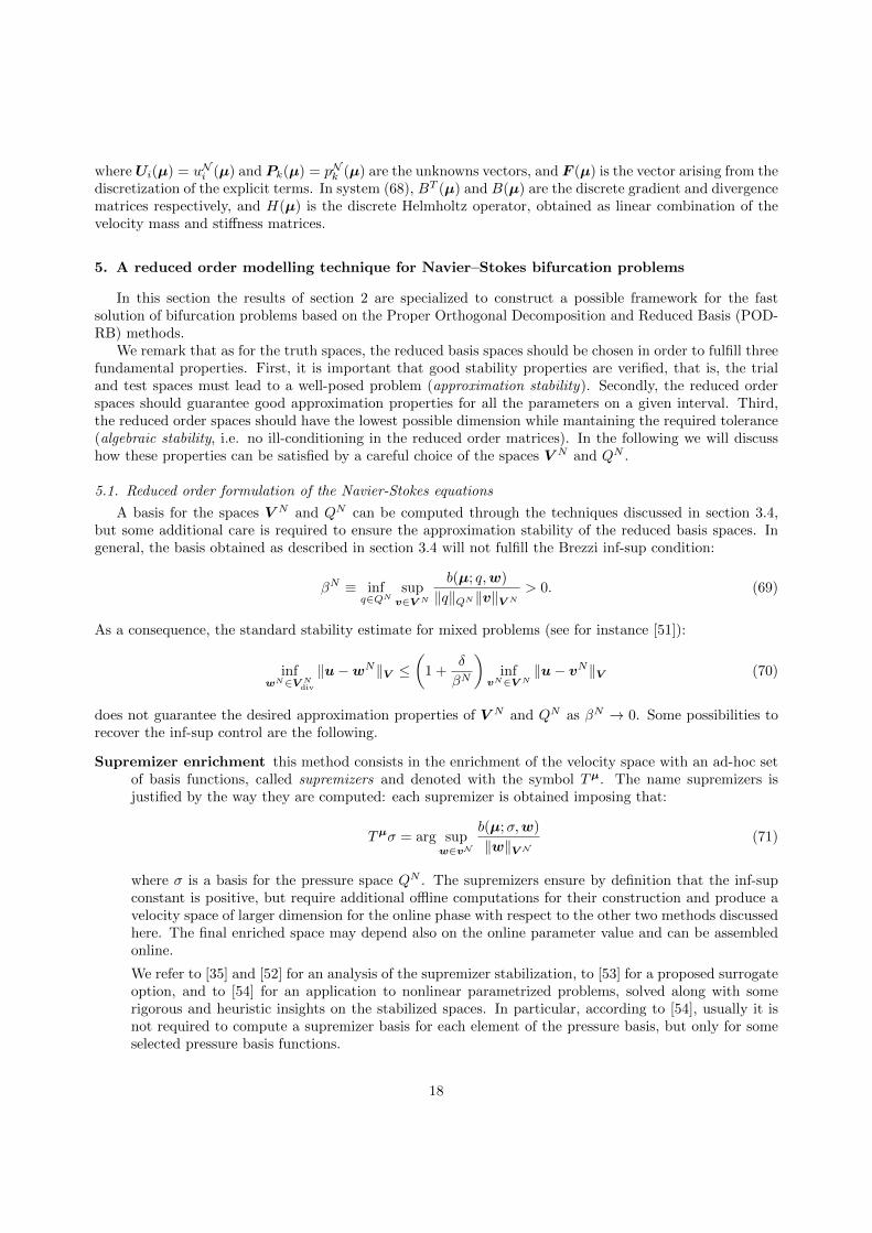
We portray in figure 3 the eigenvalues of the operator T (u∗) evaluated in a neighbourhood of a bifurcationpoint for a reduced order simulation of the cavity toy model problem. In particular, we fix an interval forthe Grashof number where there exist both a steady state and a Hopf bifurcation point for the single rollflow, and we evaluate the spectrum of the tangent operator on a basis set obtained from flows with one, twoand three rolls, and we compare it with the spectrum computed on a basis set coming from snapshots withonly two and three rolls. In the first case we can see both a steady state bifurcation (the eigenvalue crossingthe zero) and, for higher values of the Grashof number, a Hopf bifurcation (the pair of complex conjugateeigenvalues crossing the imaginary axis). In the second case no eigenvalue passes through zero or crossesthe imaginary axis, hence the second reduced basis set is not able to detect the two bifurcations.

Figure 3: Reduced Model Eigenvalues of the tangent advection operator T at the bifurcation point forA = 4, for Gr ∈ [80 · 103, 110 · 103]. On the left the tangent operator is evaluated on a basis set with one,two and three rolls, on the right a set with only two and three roll flows.

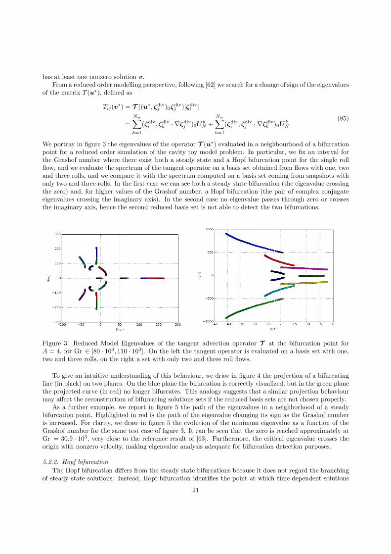
To give an intuitive understanding of this behaviour, we draw in figure 4 the projection of a bifurcatingline (in black) on two planes. On the blue plane the bifurcation is correctly visualized, but in the green planethe projected curve (in red) no longer bifurcates. This analogy suggests that a similar projection behaviourmay affect the reconstruction of bifurcating solutions sets if the reduced basis sets are not chosen properly.

As a further example, we report in figure 5 the path of the eigenvalues in a neighborhood of a steadybifurcation point. Highlighted in red is the path of the eigenvalue changing its sign as the Grashof numberis increased. For clarity, we draw in figure 5 the evolution of the minimum eigenvalue as a function of theGrashof number for the same test case of figure 3. It can be seen that the zero is reached approximately atGr = 30.9 · 103, very close to the reference result of [63]. Furthermore, the critical eigenvalue crosses theorigin with nonzero velocity, making eigenvalue analysis adequate for bifurcation detection purposes.

5.2.2. Hopf bifurcation

The Hopf bifurcation differs from the steady state bifurcations because it does not regard the branchingof steady state solutions. Instead, Hopf bifurcation identifies the point at which time-dependent solutions

21

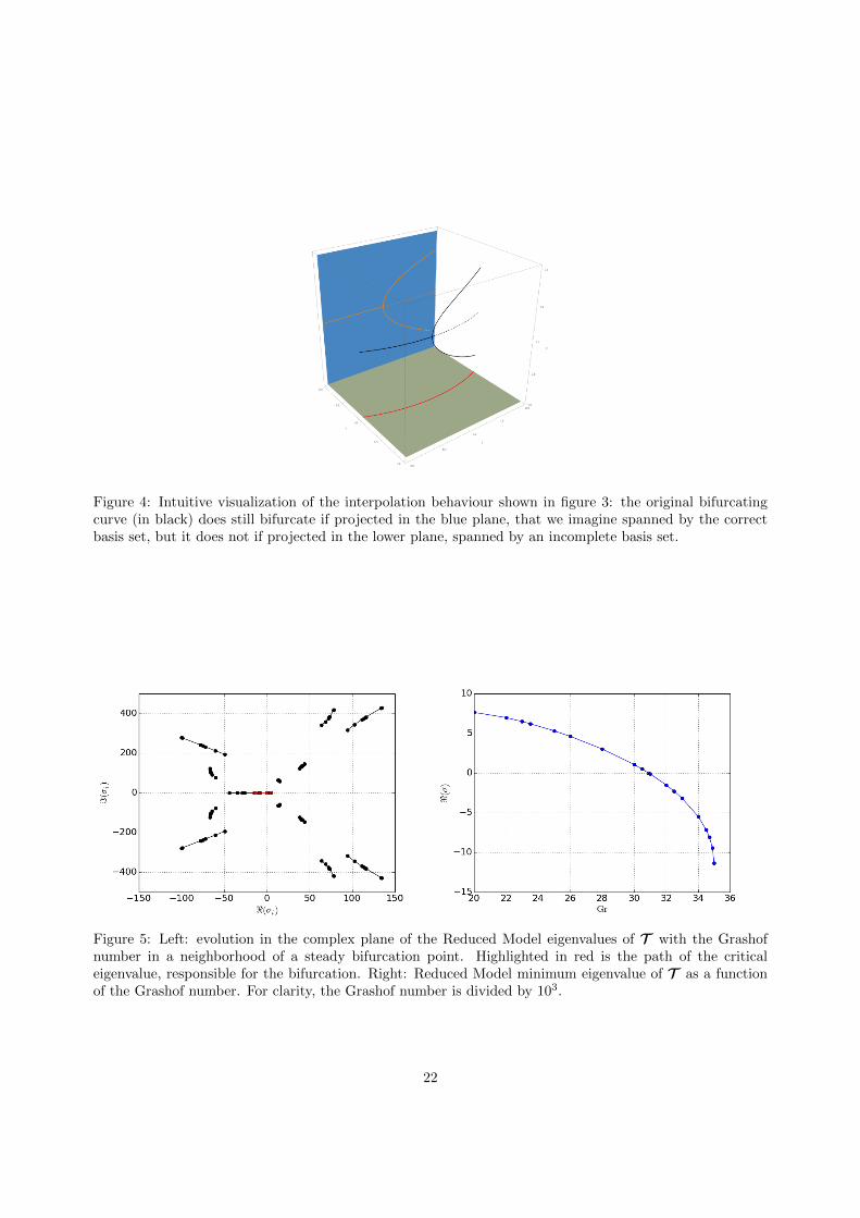
Figure 4: Intuitive visualization of the interpolation behaviour shown in figure 3: the original bifurcatingcurve (in black) does still bifurcate if projected in the blue plane, that we imagine spanned by the correctbasis set, but it does not if projected in the lower plane, spanned by an incomplete basis set.

Figure 5: Left: evolution in the complex plane of the Reduced Model eigenvalues of T with the Grashofnumber in a neighborhood of a steady bifurcation point. Highlighted in red is the path of the criticaleigenvalue, responsible for the bifurcation. Right: Reduced Model minimum eigenvalue of T as a functionof the Grashof number. For clarity, the Grashof number is divided by 103.

22

become stable. This implies that a random perturbation from a steady state does not damp off in time, butafter a transient it leads to a new, time-dependent solution.

For the detection of Hopf bifurcation points, the results of section 2.3 apply directly. We write thetime-dependent Navier-Stokes equations seeking for a solution in the form of a superposition of a steadystate solution u∗(x) and a small perturbation u′(x)eσt. Neglecting the second order terms, we obtain alinearized equation that rules the time-evolution of the perturbations:

u∗ · ∇u′ + u′ · ∇u∗ −∆u′ = −σu′ (86)

that can be seen as an eigenvalue problem for the linearized Navier-Stokes operator L : V 7→ V :

L(u∗)[u′] = −σu′. (87)

If equation (87) admits an eigenvalue σ∗ such that <σ∗ > 0, the corresponding perturbation will grow intime, and if =σ∗ > 0, an oscillatory solution has to be expected, at least until the nonlinear term u′ · ∇u′

remains sufficiently small.Applying this technique to the reduced order model, the Hopf bifurcation is detected when the matrix

L associated to the linearized Navier-Stokes operator L(u∗) admits an eigenvalue satisfying the conditionsabove. Explicitly, the matrix L has the form

Lij =

Nu∑k=1

(ζdivi , ζdiv

k · ∇ζdivj )0U

kN +

Nu∑k=1

(ζdivi , ζdiv

j · ∇ζdivk )0U

kN + (∇ζdiv

i ,∇ζdivj )0. (88)

Approximating numerically the Reduced Order Model eigenvalues of matrices (85) or (88) is not par-ticularly difficult due to their low dimension, hence direct eigenvalue algorithms can be used, such as theQR algorithm. Usually performing eigenvalue approximations of large sparse matrices arising from the sta-bility analysis of Navier-Stokes equations is a delicate task, as Arnoldi methods can compute only a feweigenvalues. We refer to [64] for a discussion on the approximation of any number of eigenvalues for largesystems.

6. Numerical results

We now test the efficiency of the reduced basis method for flow bifurcation problems on a well-knowntest case, presented at the GAMM benchmark on oscillatory convection of low Prandtl number flows, [12].Many experimental and numerical references exist on this benchmark, among which we will refer to theresults in [63].

In this benchmark the parameters are the domain length A ∈ [2, 10] and the Grashof number Gr ∈[50 · 103, 1 · 106], defined in [63] as the conventional Grashof number multiplied by the domain length A.In the considered parameter domain there exist regions admitting unique steady solutions, multiple steadysolutions, and unsteady solutions, consequently this represents a good problem to test the proposed numericalmethod.

Some representative solutions for this benchmark are shown in figure 6. As it can be seen in thevisualizations, the solutions are very heterogeneous as the Grashof number and Aspect Ratio are variedwithin D.

We choose as reference domain the rectangle with A = 2 and the affine transformation is given by:(xy

)= T aff(x, µ) =

(00

)+

[µ2 00 1

](xy

). (89)

For this simple geometry, the Piola transformation P(µ,x), is simply the inverse of Gaff(µ).Operatively, it is sufficient to compute once the reduced order matrices on the reference domainand the

right hand side vector for all the Reduced Basis functions ζdiv. Then, during the online phase, each entryof the matrices is multiplied by the corresponding Gij(µ) in order to evaluate the differential forms on the

basis set ζdivi instead of ζdiv

i .For the time evolution of the online system we chose third order semi-implicit Backward Difference

Formula (BDF3).

23

Figure 6: Some snapshots for the GAMM benchmark. From top to bottom, and from left to right: (µ =2,Gr = 50); (µ = 3.37,Gr = 264.9); (µ = 5.52,Gr = 132.1); (µ = 8.36,Gr = 50.77); (µ = 10,Gr = 100).All snapshots are steady state, except the one with three rolls.

6.1. Bifurcation diagram for A = 4

In the first test case the geometric aspect ratio is fixed to A = 4, and the snapshots are collected untilthe tolerance computed as in (27) falls below 10−4. The sampling procedure provided 13 snapshots forGr ∈ [40 · 103, 1 · 106], of which 7 are steady state solutions, and the remaining 6 are computed by a PODof 2 time periodic solutions, with an L2 energy threshold fixed to 99.9%. To test the proposed methodology(CVT-POD, SEM, Piola transformation) in the usual RB framework we try to rebuild a known bifurcationdiagram with the reduced model, with the aim to reconstruct the different solution branches.

According to [63], for this configuration there are three steady solutions up to Gr = 120 · 103, afterwhich a Hopf bifurcation occurs and the flow becomes unsteady. The three branches of steady solutionsare characterized by a single roll flow up to Gr = 25 · 103, then flows with two rolls are stable for Gr ≤100 · 103, and finally three roll flows exist from this last point up to the Hopf bifurcation. The steady stateretained snapshots are almost equally distributed between one, two and three roll flows. The time-dependentsnapshots are taken at the extreme ends of the Grashof parameter domain, very close to the Hopf bifurcationand at the Gr = 1 · 106 extreme. Both the time-dependent simulations required 3 POD modes to store the99.9% of the energy.

To build the bifurcation diagram, we performed first a reduced time-dependent simulation with anhomogeneous initial condition, and for the lowest value of the Grashof number, set at Gr = 40 · 103. Weremark again that in [63] was used a different definition for the Grashof number, hence the value to be usedfor the numerical simulations is Gr = 10 · 103. This run evolved to a steady state solution (within an L2

tolerance of 10−8), and successfully rebuilt the first snapshot, consisting in the one roll flow typical of thelow Grashof solutions.

Then, some time-dependent simulations are carried out with increasing values of the Grashof number,using as initial condition the result of the previous simulation. The continuation method has been used untilthe Hopf bifurcation was reached. Finally, the continuation method has been run backwards, with decreasingvalues of the Grashof number. The results obtained are synthesized in figure 7, where the evolution of thehorizontal velocity at a fixed point is plot as a function of the Grashof number. The three branches canclearly be identified, and some hysteresis is present, especially at the one to two rolls transition. For clarityreasons, we also plot the streamlines of some representative solutions.

Note that to build the bifurcation diagram we had to compute 24 solutions for different values of theGrashof number with, N = 13 basis functions. The online procedure required slightly less than 600 seconds,

24

while the full order run would have taken about 24 cpu-hours for each solution, thus requiring approximately576 cpu-hours to complete, on a IBM iDataPlex DX360M3 cluster. We estimate that in this way we reducedthe computation time approximately by a factor of two:

offline computation time + online computation time

equivalent fully offline computation time'

13 · 24 + 16

24 · 24= 54%,

but this savings estimate can be much better when the number of offline runs becomes large, as we shall seein the next numerical test.

Figure 7: Bifurcation diagram for an aspect ratio of 4. The graph shows the horizontal velocity at the point(0.7, 0.7) as a function of the Grashof number. The three lines are associated to the solutions with 1, 2, and3 rolls, and the streamlines of some representative solutions are plotted for clarity.

6.2. Stability regions

After the satisfactory results of the fixed-geometry test, we consider the more general case with parametrizedgeometry. The parameter space D is now two dimensional, in particular we choose Gr ∈ [50 · 103, 1 · 106]and A ∈ [2, 6].

At first, we collect a sufficient set of snapshots to extract the information needed for the online phase. Westart from a set of 5 snapshots, corresponding to the four vertices and the center of the parameter rectangleD. Such snapshots are used as a starting set for the CVT sampling procedure exposed in section 3.2. Forthe sake of clarity, we report a scheme of the actual algorithm (Algorithm 2).

We remark that the sampling procedure exposed in Algorithm 2 is divided between two basis sets: one forthe steady snapshots and another for the time-dependent snapshots. This separation is necessary because,due to the time averaging errors, the tolerance of the steady state snapshots as computed in equation (91)is an order of magnitude lower than the tolerance for the time-dependent snapshots. If the CVT wereperformed without this precaution, the steady state regions of D would be heavily underrepresented, orconversely the number of time-dependent snapshots would be too large. The selection of suitable tolerancecriteria for the two sampling procedures is a difficult task, and we chose to set the two tolerance valuestreating the steady-state and time-dependent cases as separate, imposing tolerances based on experienceand on the realizable error bounds.

In this test, the sampling provided a total of 108 basis functions, arising from 30 steady and 21 unsteadysnapshots. Almost all the unsteady snapshots required 3 POD modes to store the 99.9% of the energy,except for a few cases where 2 modes were enough. We report in figure 8 the position of the snapshots onthe parameter plane (A,Gr ), as computed by the Algorithm 2 (CVT).

As a basic validation for the online solver, we run several online simulations with all the 108 basisfunctions, for the parameters µi used for the snapshot computation where the solution is known to beunique. The steady state snapshots have been correctly rebuilt by the online simulation, with L2 differencesbetween the snapshots and their online reconstruction alway of the order of the sampling tolerance.

25

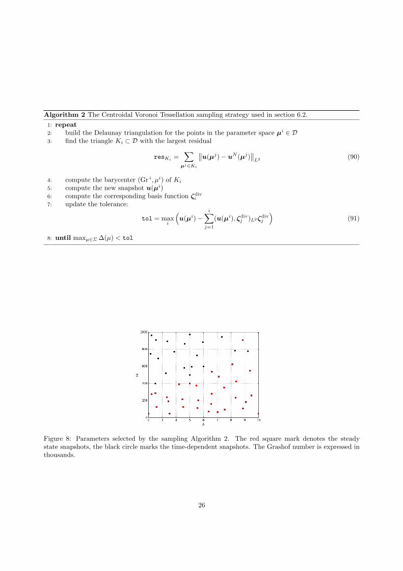
Algorithm 2 The Centroidal Voronoi Tessellation sampling strategy used in section 6.2.

1: repeat2: build the Delaunay triangulation for the points in the parameter space µi ∈ D3: find the triangle Ki ⊂ D with the largest residual

resKi=∑µj∈Ki

∥∥u(µj)− uN (µj)∥∥L2 (90)

4: compute the barycenter (Gr i, µi) of Ki

5: compute the new snapshot u(µi)6: compute the corresponding basis function ζdiv

i

7: update the tolerance:

tol = maxi

(u(µi)−

i∑j=1

(u(µi), ζdivj )L2ζdiv

j

)(91)

8: until maxµ∈Σ ∆(µ) < tol

Figure 8: Parameters selected by the sampling Algorithm 2. The red square mark denotes the steadystate snapshots, the black circle marks the time-dependent snapshots. The Grashof number is expressed inthousands.

26

On the other hand, the unsteady simulations show some discrepancies with the snapshots in terms of theoscillation’s frequency, but the L2 difference between the average values of the offline and online simulationare of the same order of magnitude of the sampling tolerance. We suspect that the frequency discrepancyof the online phase should be ascribed to the absence of the rejected POD modes that could be responsiblefor the frequency drift.

Despite the frequency drift during the online phase, the behaviour of the Hopf bifurcation frequencyshows the expected decay as the geometry is varied. In figure 9, we plot the frequency at the onset of Hopfbifurcation for the one, two and three roll cases, as a function of the cavity length A. The asymptotic decayis confirmed by the benchmark [63], and is physically justified since for longer cavities the stability area ofone roll flows shrinks to very low Grashof numbers, and consequently the flow must happen at a low velocityin order to mantain the stability of this very long vortex. Also, we note that sudden changes in the stabilityarea happening about A = 4.8 in figure 10 are reflected by the abrupt change of sign of the derivative of thered curve in figure 9.

2.0 2.5 3.0 3.5 4.0 4.5 5.0 5.5 6.0A

0

20

40

60

80

100

120

140

160

f

Figure 9: Frequency f = 1/ω at the onset of the periodic solution as a function of the geometric aspect factorA. The one roll solutions are marked in black, the two rolls solutions in red and the three rolls solutions inblue.

In particular, a remarkable feature of the online phase is that the basis arising from snapshots thatare physically impossible for a certain flow configuration are cancelled out by the Galerkin projection. Forinstance, if we fix A = 4, the only admissible solutions for this geometry display one, two, or three rolls, andthe basis arising from four or five rolls snapshots are automatically excluded by the online projection (thecorresponding coefficients begin very close to machine zero).

Next, we investigate the stability of the reduced basis solutions using the techniques exposed in sec-tion 5.2, with the goal of identifying the stability regions of each flow pattern. In particular, we areinterested in finding the curves in the parameters’ plane that limit the stability of steady flows with one,two, three or four rolls. These curves are formed either by an envelope of steady bifurcation points or Hopfbifurcation points.

First, we compute the Hopf bifurcation point for a series of values of A ∈ [2, 6]. We adopt a subset of the108 basis consisting of the 25 basis with a single roll. At each run a continuation method on Gr is used, andthe reduced system is evolved until a new steady state is reached, with the modulus of the time derivativebelow a tolerance of 10−8. After the steady solution is reached, the eigenvalues of the reduced linearizedNavier-Stokes operator (88) are computed, and the Hopf bifurcation is marked for the Gr whose maximumeigenvalues have a real part sufficiently close to zero.

This operation is repeated for the solution branch with two roll basis (of dimension 14), and for the threeand four roll branches (dimension 22 and 9 respectively). For each subset, the geometry parameter A rangeis bounded below by the snapshot with the lowest value of A.

Then, we compute the steady state bifurcations by running reduced order simulations using basis sets

27

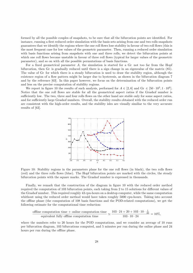
formed by all the possible couples of snapshots, to be sure that all the bifurcation points are identified. Forinstance, running a first reduced order simulation with the basis sets arising from one and two rolls snapshotsguarantees that we identify the regions where the one roll flows lose stability in favour of two roll flows (this isthe most frequent case for low values of the geometric parameter. Then, running a reduced order simulationwith basis functions arising from snapshots with one and three rolls, we detect the bifurcation points atwhich one roll flows become unstable in favour of three roll flows (typical for larger values of the geometricparameter), and so on with all the possible permutations of basis functions.

For a fixed geometrical parameter A, the simulation is started for a Gr not too far from the Hopfbifurcation, then Gr is gradually reduced until there is a sign change in an eigenvalue of the matrix (85).The value of Gr for which there is a steady bifurcation is used to draw the stability region, although theexistence region of a flow pattern might be larger due to hysteresis, as shown in the bifurcation diagram 7and by the reference [63]. In this paper however, we focus on the determination of the bifurcation pointsand less on the precise computation of stability regions.

We report in figure 10 the results of such analysis, performed for A ∈ [2, 6] and Gr ∈ [50 · 103, 1 · 106].Notice that the one roll flows are stable for all the geometrical aspect ratios if the Grashof number issufficiently low. The two, three and four rolls flows on the other hand are stable only for some aspect ratios,and for sufficiently large Grashof numbers. Overall, the stability results obtained with the reduced order runare consistent with the high-order results, and the stability isles are visually similiar to the very accurateresults of [63].

Figure 10: Stability regions in the parameters plane for the one roll flows (in black), the two rolls flows(red) and the three rolls flows (blue). The Hopf bifurcation points are marked with the circles, the steadybifurcation points with the square marks. The Grashof number is expressed in thousands.

Finally, we remark that the construction of the diagram in figure 10 with the reduced order methodrequired the computation of 103 bifurcation points, each taking from 2 to 15 solutions for different values ofthe Grashof number. This required roughly 43 cpu-hours on a desktop computer, while the same computationwhithout using the reduced order method would have taken roughly 5000 cpu-hours. Taking into accountthe offline phase (the computation of 108 basis functions and the POD-related computations), we get thefollowing estimate for the computational time reduction:

offline computation time + online computation time

equivalent fully offline computation time'

103 · 24 + 20 + 103 · 10 · 120

103 · 10 · 24= 10%,

where the numbers refer to 20 hours for the POD computations, and we consider an average of 10 runsper bifurcation diagram, 103 bifurcations computed, and 5 minutes per run during the online phase and 24hours per run during the offline phase.

28

6.3. Time-dependent results

Finally, the accuracy of the ROM is tested with a time-dependent benchmark. For this purpose, wecompare the results of the high order simulation with the results of the ROM simulation for some represen-tative values of the parameters. In particular, we focus on time-periodic simulations with all the possibleflow structure in the parameter range considered in this work. Specifically, we simulate parameter valuesfor which a flow structure spanning from one to four vortices is expected.

For each simulation a basis is built starting from the snapshots with the same number of vortices. Inall cases, the reduced order simulations converge to the expected periodic solution. In figure 11 is draw acomparison of the horizontal velocity at a fixed point as a function of time, as computed with a high ordersimulation, and with the reduced order approximation. We remark that the reduced order dynamics is ingood agreement with the high-order dynamics in terms of average value, oscillation amplitude and frequency.In particular, for the considered test case the relative error in oscillation frequency of the reduced model isquantified in 0.51%.

The computational reduction is also relevant, since the reduced order simulation takes less than 5 minuteson a personal computer, whereas the high-resolution simulation requires 24 cpu-hours on the CINECA PLXcluster (an IBM iDataPlex DX360M3).

Figure 11: Comparison of the horizontal velocity at a the point (0.7, 0.7) vs time for the high order (in red,HO) and reduced order (in black, RO) simulations. The parameters are Gr = 963791, A = 2.22, and theresulting flow has a single roll.

7. Perspectives

This work highlights several improvements with respect to the state of the art for parametrized viscousflow stability and bifurcation problems approached with ROM: in particular the focus has been put onapproximation stability, proper sampling techniques and reduced eigenproblems for stability analysis andbifurcations detection. The exposition presents the topic from the different viewpoints of Nonlinear Math-ematical Analysis, Applied Mathematics and Numerical Analysis, trying to underline the different aspectsof the problem under consideration and by bridging these studies with offline high performance computing,on one side, and online advanced reduced order modelling, on the other one. Tests were performed on awell-known cavity benchmark problem.

We plan to extend the proposed ROM framework to more advanced 3D problems, in particular withapplications to the study of the Coanda effect in hemodynamics [65], and the influence of geometry onsymmetry breaking. More complex studies may be devoted to bifurcations and stability of flows with anelastic wall-structure interaction.

29

Acknowledgements

The authors acknowledge Dr. E. Merzari for his help with the Nek5000 software and for the usefuldiscussions, and the Nek5000 community in general, Dr. F. Ballarin for the insights on approximationstability. G. Pitton has been supported by the pre-doc program at SISSA. G. Rozza acknowledges the supportof NOFYSAS excellence grant program at SISSA and INDAM-GNCS activity group. The motivation fordeveloping this work came from Prof. A.T. Patera (MIT) and from Prof. J. Rappaz (EPFL). We acknowledgeProf. F. Brezzi (IUSS, Pavia) for insights and some references.

We gratefully thank Prof. A. Quaini for ongoing collaboration on this topic with the MathematicsDepartment at University of Houston, USA.

The computing resources have been provided by the Sis14 COGESTRA cpu time grant allocation atCINECA, Bologna, Italy.

References

[1] A. Ambrosetti, G. Prodi, A Primer of Nonlinear Analysis, Cambridge University Press, Cambridge, 1993.[2] S. Chandrasekhar, Hydrodynamic and Hydromagnetic Stability, Dover Publications, 1982.[3] S. Timoshenko, J. Gere, Theory of Elastic Stability, Dover Civil and Mechanical Engineering, Dover Publications, 2009.[4] J. Marsden, T. Hughes, Mathematical Foundations of Elasticity, Dover Civil and Mechanical Engineering, Dover Publi-

cations, 1994.[5] G. Rozza, D. Huynh, A. Patera, Reduced basis approximation and a posteriori error estimation for affinely parametrized

elliptic coercive partial differential equations, Archives of Computational Methods in Engineering 15 (3) (2008) 229–275.[6] P. Holmes, J. Lumley, G. Berkooz, C. Rowley, Turbulence, Coherent Structures, Dynamical Systems and Symmetry,

Cambridge University Press, Cambridge, 2012.[7] F. Terragni, J. Vega, On the use of POD-based ROMs to analyze bifurcations in some dissipative systems, Physica D:

Nonlinear Phenomena (241.17) (2012) 1393–1405.[8] H. Herrero, Y. Maday, F. Pla, RB (Reduced Basis) for RB (Rayleigh-Benard), Computer Methods in Applied Mechanics

and Engineering (261-262) (2013) 132–141.[9] M. Yano, A. Patera, A space-time variational approach to hydrodynamic stability theory, Proceedings of the Royal Society

A (496.2155).[10] T. Lassila, A. Manzoni, A. Quarteroni, G. Rozza, Model order reduction in fluid dynamics: challenges and perspectives, in:

A. Quarteroni, G. Rozza (Eds.), Reduced Order Methods for modeling and computational reduction, Vol. 9 of Modeling,Simulation and Applications, Springer, Milano, 2014, Ch. 9, pp. 235–273.

[11] A. Noor, J. Peters, Multiple-parameter reduced basis technique for bifurcation and post-buckling analyses of compositemateriale, International Journal for Numerical Methods in Engineering (19) (1983) 1783–1803.

[12] B. Roux (Ed.), Numerical Simulation of Oscillatory Convection in Low-Pr Fluids, Vol. 27 of Notes on Numerical FluidMechanics and Multidisciplinary Design, Springer, 1990.

[13] A. Ambrosetti, A. Malchiodi, Nonlinear Analysis and Semilinear Elliptic Problems, Cambridge University Press, Cam-bridge, 2007.

[14] G. Caloz, J. Rappaz, Numerical analysis for nonlinear and bifurcation problems (1997).[15] F. Brezzi, J. Rappaz, P. Raviart, Finite Dimensional Approximation of Nonlinear Problems. Part I: Branches of Nonsin-

gular Solutions, Numerische Mathematik 36 (1) (1980) 1–25.[16] F. Brezzi, J. Rappaz, P. Raviart, Finite Dimensional Approximation of Nonlinear Problems. Part II: Limit Points, Nu-

merische Mathematik 37 (1) (1981) 1–28.[17] F. Brezzi, J. Rappaz, P. Raviart, Finite Dimensional Approximation of Nonlinear Problems. Part III: Simple Bifurcation

Points, Numerische Mathematik 38 (1) (1982) 1–30.[18] S. P. Singh, M. R. Singh, Best approximation in nonlinear functional analysis, in: Q. Ansari (Ed.), Nonlinear Analysis,

Trends in Mathematics, Springer, 2014, pp. 165–198.[19] G. Golub, C. V. Loan, Matrix Computations, Johns Hopkins University Press, 2012.[20] A. Quarteroni, A. Valli, Domain Decomposition Methods for Partial Differential Equations, Numerical Mathematics and

Scientific Computation, Oxford University Press, 1999.[21] A. Toselli, O. Widlund, Domain Decomposition Methods — Algorithms and Theory, Vol. 34 of Springer Series in Com-

putational Mathematics, Springer Berlin Heidelberg, 2005.[22] H. Dijkstra, F. Wubs, A. Cliffe, E. Doedel, I. Dragomirescu, B. Eckhardt, A. Gelfgat, A. Hazel, V. Lucarini, A. Salinger,

E. Phipps, J. Sanchez-Umbria, H. Schuttelaars, L. Tuckerman, U. Thiele, Numerical bifurcation methods and their appli-cation to fluid dynamics: Analysis beyond simulation, Communications in Computational Physics 15 (1) (2014) 1–45.

[23] V. Temlyakov, Greedy approximation, Acta Numerica 17 (2008) 235–409.[24] P. Binev, A. Cohen, W. Dahmen, R. DeVore, G. Petrova, P. Wojtaszczyk, Convergence rates for greedy algorithms in

reduced basis methods, SIAM Journal on Mathematical Analysis 43 (3) (2011) 1457–1472.[25] A. Buffa, Y. Maday, A. Patera, G. Turinici, A priori convergence of the greedy algorithm for the parameterized reduced

basis, ESAIM Mathematical Modelling and Numerical Analysis 46 (3) (2011) 595–603.

30

[26] Q. Du, M. Gunzburger, Model reduction by proper orthogonal decomposition coupled with centroidal voronoi tessellation,in: Proceedings of Fluids Engineering Division Summer Meeting, Vol. 1, ASME, 2002.

[27] Q. Du, M. Gunzburger, Centroidal voronoi tessellation based proper orthogonal decomposition analysis, Birkhauser Basel,2003.

[28] M. Bergmann, T. Colin, A. Iollo, D. Lombardi, O. Saut, H. Telib, Reduced Order Models at Work in Aeronautics andMedicine, in: A. Quarteroni, G. Rozza (Eds.), Reduced Order Methods for Modeling and Computational Reduction, Vol. 9of Modeling, Simulation and Applications, Springer, Milano, 2014.

[29] K. Ito, S. Ravindran, A reduced order method for simulation and control of fluid flows, Journal of Computational Physics143 (2) (1998) 403–425.

[30] S. Volkwein, Proper orthogonal decomposition: Theory and reduced-order modelling (2013).[31] B. Haasdonk, M. Ohlberger, Reduced basis method for finite volume approximations of parametrized linear evolution

equations, ESAIM Mathematical Modelling and Numerical Analysis 42 (2) (2008) 277–302.[32] N. Nguyen, G. Rozza, A. Patera, Reduced basis approximation and a posteriori error estimation for the time-dependent

viscous burgers’ equation, Calcolo 46 (2009) 157–185.[33] P. Schmid, Dynamic mode decomposition of numerical and experimental data, Journal of Fluid Mechanics 656 (2010)

5–28.[34] M. Barrault, Y. Maday, N. Nguyen, A. Patera, An “empirical interpolation method”: application to efficient reduced-basis

discretization of partial differential equations, C. R. Acad. Sci. Paris, Ser. I 339 (2004) 667–672.[35] G. Rozza, K. Veroy, On the stability of the reduced basis method for Stokes equations on parametrized domains, Computer

methods in applied mechanics and engineering (196) (2007) 1244–1260.[36] Y. Saad, Iterative Methods for Sparse Linear Systems, SIAM, 2003.[37] Y. Saad, Numerical Methods for Large Eigenvalue Problems, Revised Edition, Vol. 66 of Classics in Applied Mathematics,

SIAM, 2011.[38] N. Grabner, S. Quraishi, C. Schroder, V. Mehrmann, U. von Wagner, New numerical methods for the complex eigenvalue

analysis of disk brake squeal, in: EuroBrake 2014 Conference Proceedings, 2014.[39] K. Veroy, A. Patera, Certified real-time solution of the parametrized steady incompressible navier-stokes equations: rig-

orous reduced-basis a posteriori error bounds, International Journal for Numerical Methods in Fluids 47 (8-9) (2005)773–788.

[40] S. Deparis, G. Rozza, Reduced basis method for multi-parameter dependent steady navier-stokes equations: applicationsto natural convection in a cavity, Journal of Computational Physics 228 (12) (2009) 4359–4378.

[41] D. Huynh, G. Rozza, S. Sen, A. Patera, A successive constraint linear optimization method for lower bounds of parametriccoercivity and inf–sup stability constants, Comptes Rendus Mathematique 345 (8) (2007) 473–478.

[42] F. Brezzi, M. Cornalba, A. D. Carlo, How to get around a simple quadratic fold, Numerische Mathematik 48 (1986)417–427.

[43] K. Urban, A. Patera, A new error bound for reduced basis approximation of parabolic partial differential equations,Comptes Rendus Mathematique 350 (3-4) (2012) 203–207.

[44] L. Evans, Partial Differential Equations, Vol. 19 of Graduate Studies in Mathematics, American Mathematical Society,2010.

[45] L. Landau, E. Lifshitz, Fluid Mechanics, Vol. 6 of Course of Theoretical Physics, Butterworth Heinemann, Oxford, 1987.[46] M. Deville, P. Fischer, E. Mund, High-Order Methods for Incompressible Fluid Flow, Cambridge Monographs on Applied

and Computational Mathematics, Cambridge University Press, Cambridge, 2002.[47] C. Canuto, M. Hussaini, A. Quarteroni, T. Zhang, Spectral Methods Fundamentals in Single Domains, Scientific Compu-

tation, Springer, 2006.[48] C. Canuto, M. Hussaini, A. Quarteroni, T. Zhang, Spectral Methods Evolution to Complex Geometries and Applications

to Fluid Dynamics, Scientific Computation, Springer, 2007.[49] P. Fischer, J. Lottes, S. Kerkemeier, Nek5000 Web page, http://nek5000.mcs.anl.gov (2008).[50] A. Tomboulides, J. Lee, S. Orszag, Numerical Simulation of Low Mach Number Reactive Flows, Journal of Scientific

Computing 12 (2) (1997) 139–167.[51] D. Boffi, F. Brezzi, M. Fortin, Mixed Finite Element Methods and Applications, Vol. 44 of Springer Series in Computational

Mathematics, Springer, Heidelberg, 2013.[52] G. Rozza, D. Huynh, A. Manzoni, Reduced basis approximation and a posteriori error estimation for Stokes flows in

parametrized geometries: roles of the inf—sup stability constants, Numerische Mathematik 125 (1) (2013) 115–152.[53] A.-L. Gerner, K. Veroy, Certified reduced basis methods for parametrized saddle point problems, SIAM Journal on

Scientific Computing 34 (5) (2012) A2812–A2836.[54] F. Ballarin, A. Manzoni, A. Quarteroni, G. Rozza, Supremizer stabilization of POD-Galerkin approximation of

parametrized Navier-Stokes equations, International Journal for Numerical Methods in Engineering (13).[55] D. Rovas, Reduced-basis output bound methods for parametrized partial differential equations, Ph.D. thesis, Massachusetts

Institute of Technology (2003).[56] D. Amsallem, C. Farhat, Stabilization of projection-based reduced-order models, International Journal for Numerical

Methods in Engineering 91 (2012) 358–377.[57] W. Dahmen, How to best sample a solution manifold?, in: G. Pfander (Ed.), Sampling Theory - a Renaissance, Applied

and Numerical Harmonic Analysis, Springer-Birkhauser, 2015.[58] A. Abdulle, O. Budac, A petrov-galerkin reduced basis approximation of the Stokes equation in parametrized geometries,

Tech. Rep. MATHICSE Technical Report 35.2014, Ecole polytechnique federale de Lausanne (aug 2014).[59] A. Løvgren, Y. Maday, E. Rønquist, A reduced basis element method for the steady stokes problem, ESAIM: Mathematical

31

Modelling and Numerical Analysis 40 (3) (2006) 529–552.[60] A. Caiazzo, T. Iliescu, J. Volker, S. Schyschlowa, A numerical investigation of velocity–pressure reduced order models for

incompressible flows, Journal of Computational Physics 259 (2014) 598–616.[61] G. Galdi, Navier-Stokes Equations: a Mathematical Analysis, in: R. Meyers (Ed.), Mathematics of Complexity and

Dynamical Systems, Springer, 2011, pp. 1009–1042.[62] K. Cliffe, E. Hall, P. Houston, E. Phipps, A. Salinger, Adaptivity and a Posteriori Error Control for Bifurcation Problems

III: Incompressible Fluid Flow in Open Systems with O(2) Symmetry, Journal of Scientific Computing 52 (1) (2012)153–179.

[63] A. Gelfgat, P. Bar-Yoseph, A. Yarin, Stability of multiple steady states of convection in laterally heated cavities, Journalof Fluid Mechanics (388) (1999) 315–334.

[64] H. Elman, K. Meerbergen, A. Spence, M. Wu, Lyapunov Inverse Iteration for Identifying Hopf Bifurcations in Models ofIncompressible Flow, SIAM Journal on Scientific Computing 34 (3) (2012) A1584–A1606.

[65] A. Quaini, R. Glowinski, S. Canic, Symmetry breaking and Hopf bifurcation for incompressible viscous flow in acontraction-expansion channel, submitted, University of Houston, Dept. of Math. Technical Report, 2014.

32