Realisation of the Use of Computational Model as Part of ...

Realisation of the Use of Computational

Model as Part of TKA Surgical Planning

by

Willy Theodore

Thesis

Submitted to Flinders University

for the degree of

Doctor of Philosophy

College of Science and Engineering

August 2019

i

CONTENTS

Summary ....................................................................................................................................... iii

Declaration ..................................................................................................................................... v

Acknowledgements ....................................................................................................................... vi

Introduction ................................................................................................................................... 1

Chapter 1 ....................................................................................................................................... 5

Anatomy of the knee .......................................................................................................................... 5

Biomechanics of the Knee ................................................................................................................... 9

Knee Joint Pathology ......................................................................................................................... 26

Treatments Options .......................................................................................................................... 27

Total Knee Arthroplasty .................................................................................................................... 28

Outcomes of TKA .............................................................................................................................. 41

Computational Modelling ................................................................................................................. 47

Summary ........................................................................................................................................... 53

Chapter 2 ...................................................................................................................................... 56

Introduction ...................................................................................................................................... 57

Materials and Methods ..................................................................................................................... 58

Results ............................................................................................................................................... 67

Discussion ......................................................................................................................................... 73

Conclusions ....................................................................................................................................... 76

Chapter 3 ...................................................................................................................................... 77

Introduction ...................................................................................................................................... 79

Methods ............................................................................................................................................ 81

Accuracy testing ................................................................................................................................ 85

Results ............................................................................................................................................... 87

Discussion ......................................................................................................................................... 93

Conclusion ......................................................................................................................................... 97

Chapter 4 ...................................................................................................................................... 98

Introduction ...................................................................................................................................... 99

Method ........................................................................................................................................... 101

Results ............................................................................................................................................. 109

Discussion ....................................................................................................................................... 115

Conclusions ..................................................................................................................................... 119

Chapter 5 .................................................................................................................................... 120

Introduction .................................................................................................................................... 121

Method ........................................................................................................................................... 123

ii

Results ............................................................................................................................................. 129

Discussion ....................................................................................................................................... 134

Chapter 6 .................................................................................................................................... 140

Introduction .................................................................................................................................... 141

Method ........................................................................................................................................... 143

Results ............................................................................................................................................. 148

Discussion ....................................................................................................................................... 153

Chapter 7 .................................................................................................................................... 160

Summary of Key Results .................................................................................................................. 164

Development of TKR computational model with balanced technical complexity and clinical practicality ....................................................................................................................................... 169

Clinical application of current model .............................................................................................. 173

Further application to help managing patient clinical outcomes ................................................... 180

Use of Computational model as medical device ............................................................................. 181

Realising TKA computational model for clinical use ....................................................................... 182

Concluding remarks ........................................................................................................................ 185

Appendices ................................................................................................................................. 187

Appendix A ‐ First Computational Model Experimental Validation ................................................ 187

Appendix B ‐ Verification of 3D‐2D Registration technique using Sawbone Model ....................... 192

References .................................................................................................................................. 203

iii

Summary

Total Knee Arthroplasty (TKA), despite being a highly successful medical operation when measured in

terms longevity, has a recurrent problem of patient dissatisfaction and complications in the range of

15‐20%. Patient satisfaction is known to be a complex multifactorial issue with factors such as implant

component position, pain relief, functionality or stability after surgery, patient expectation, other co‐

morbidities, experience of healthcare delivery. These factors can be largely grouped into surgical

factors, patient factors and patient management factors. With the extensive variation between

patients, clinicians need tools to help them triage patients, helping them make decision what

resources needed to treat individual patient to achieve the best possible outcome for the patient while

minimizing the healthcare cost. Surgical planning is one key aspect that can help clinicians better

choose options for surgery.

Joint dynamics has been shown to influence clinical outcomes and is a result of complex interactions

between the implant component design, component alignment, and patient specific anatomic

characteristics. The relationship between these factors is not well understood and computational

modelling is a scalable technique compared to other functional techniques that allow the study of

both surgical and patient factors impact on joint dynamics following TKA. A computational model

needs to have the right balance between complexity and practicality to be used in clinical setting.

This thesis presented a series of studies towards the development of a low‐cost knee computational

model that could be used to predict the clinical outcome of TKA on knee dynamics in clinical setting.

The first half of this thesis discussed the development and validation technique used for the model.

New registration techniques were developed to ensure the definition of reference frames between

in‐vitro and in‐silico environment during validation is consistent. This was often overlooked in previous

computational model validation studies. The computational model developed was able to complete a

simulation cycle within few minutes while achieving great agreement with experimental data.

iv

The second half of this thesis explored new non‐invasive techniques to incorporate subject specific

ligament properties into the developed model. Stress radiographs were used as surrogate of the load‐

displacement response of the knee and ligament properties were optimized to match the response. A

wide variation in optimized parameters between subjects and ligaments were seen however its effects

to the model dynamics is not yet well understood.

Lastly, this thesis discussed the work involved in realising the use of developed computational model

as medical device. The low‐cost knee computational model developed in this thesis was successfully

registered as medical device and has been used in clinical setting. The model has been used to analyse

approximately 1,800 post‐operative complications and over 3,000 TKA pre‐operative planning. In

conclusion, with the right balance between complexity and practicality, it is possible to use

computational modelling as part of TKA surgical planning.

v

Declaration

I certify that this thesis does not incorporate without acknowledgment any material previously

submitted for a degree or diploma in any university; and that to the best of my knowledge and belief

it does not contain any material previously published or written by another person except where due

reference is made in the text.

Signed

Date 09‐Apr‐2019

vi

Acknowledgements

Firstly, I would like to express my sincere gratitude to my advisor Prof. Mark Taylor for the continuous

support of my PhD study and related research, for his patience, motivation, and immense knowledge.

Your guidance helped me to find balance between my competing professional commitments and

research work. I could not have imagined having a better advisor and mentor for my PhD study. I

would also like to thank Flinders University and its helpful staff for all the guidance and support

provided to external research student.

My sincere thanks also go to Brad Miles and Bede O’Connor for the time, ideas and funding that have

gone into my PhD work. You have always been there when I need extra motivation to keep me going.

Your vision in marrying the academia and commercial reality to improve patient quality of life has led

the completion of this PhD and its application in clinical setting.

Thank you to every Orthopaedic surgeon I have ever had the honour of working with and learning

from. The clinical insights provided are tremendous to keep this PhD clinically relevant. A special thank

you to David Liu, David Dickison, Jonathan Bare, Stephen McMahon, Justin Roe, Brett Fritsch, Michael

Solomon, Richard Boyle, David Parker, and Andrew Shimmin. Your willingness to try new ideas and

sacrifice time for discussion has been humbling to witness.

Thank you to Scripps Biomechanical lab and Cleveland clinic Biomechanical lab for the support of the

experimental studies. Your patience and willingness for back‐and‐forth iteration is fundamental in

setting the ground work for this thesis.

Thank you to all of my colleagues, past and present at 360 Knee Systems and Optimized Ortho

throughout the years. Special mentions to Joe Little, Joshua Twiggs, Andy Li, Kevin Wong, Edgar

Wakelin, and linda Tran for the insights and encouragements, but also for the hard question which

incented me to widen my research from various perspectives.

Last but not the least, I would like to thank my family. Words cannot express how grateful I am to my

parents for their mental support. Thank you to my brothers, Andri and Ricky for the constant support.

1

Introduction

The knee is one of the most complex joints in the body, it has the important function of providing

support and mobility during standing and gait. It has a role in almost all daily activities and hence,

susceptible to failure particularly degenerative joint diseases like osteoarthritis.

When a knee has lost functionality due to trauma and/or disease, it may require to be managed by

means of Total Knee Arthroplasty (TKA). Due to worldwide aging population, the use of TKA has

increased steadily every year, especially in individuals younger than 65 years of age [1]. The aim of

TKA is to provide substantial relief from pain and functional improvement in patients with arthritis.

Although, TKA is considered one of the most successful operations, there are still complications and

around 20% of patients are dissatisfied with their outcome. [2]. Furthermore, due to a lack of

standardisation and validity of adequate outcome measures, it is difficult to determine which

elements before, during and after surgery; and throughout the rehabilitation process affect the

outcomes of TKA. However, with the evolution of patient centred care, technological advances in

hardware and software, there is an opportunity to combine clinical and biomechanical data collected

prior, during and after surgery with computational modelling and data analytics to find patterns or

combinations of factors that affect outcomes of TKA. Clinical and biomechanical data include

radiography imaging, knee joint assessment, subjective scores, implant geometry used, soft tissue

state, patient co‐morbidities and mental state. Understanding the combination of these factors may

provide insights to improve patient management from surgical planning to rehabilitation programs

and, as a consequence, the overall outcome for each individual patient.

This thesis aimed to present a series of studies towards the development of a computational model

that intended to be used as part of surgical planning tool to help clinicians triage patient treatments.

This includes the development and validation of a patient specific TKA computational model and a

2

clinical approach to quantify patient specific ligament characteristics that can be incorporated in the

model. This thesis will follow the structure outlined below.

Chapter 1: Literature review ‐ presents the literature review of the anatomy, physiology and relevant

pathology of the knee joint, the surgical options for intervention and existing computational modelling

technique for TKA.

Chapter 2: Variability in Static Alignment and Kinematics for Kinematically Aligned TKA – This

chapter presents the development of a simplified computational model of the knee replicating a

mechanical simulator and its ability to differentiate simulated kinematics between mechanically and

kinematically aligned components. This chapter shows the potentials of simplified computational

model can be used as part of surgical planning. Kinematic and mechanical alignments captured in this

chapter are only used as generalisations of the alignment philosophies the surgeon would normally

follow. The aim of this chapter is to show the potential of simplified computational models to

differentiate kinematics characteristics of different component alignments. This does not indicate the

model is limited to only simulate mechanical and kinematic alignment.

Chapter 3: Accurate Determination of Post‐operative 3D Component Positioning in Total Knee

Arthroplasty: The AURORA Protocol – Following from chapter 2, it was later realised there was

inconsistency in registration technique used to transform the experimental outputs to computational

model reference frame in model validation. This chapter describes a new technique to measure post‐

operative component position from Computed Tomography (CT). The technique developed involves

registering both implant and preoperative bone 3D CT segmented models to a postoperative CT

reference frame. Doing so allowed for a more accurate definition of component placement in all 3

planes, going beyond what 2D radiography can provide. While not the primary author of this paper,

my contribution to the publication includes the conception of the registration technique, development

of the step‐by‐step instructions, designed and supervised the reproducibility study. In addition, I

assisted in writing and reviewing the manuscript. I contributed 70% to the research design, 50% on

3

data collection and 50% of manuscript preparation and review. Permission from the primary author

has been provided.

Chapter 4: A Technique for Accurate Kinematic Validation of a Low‐cost Subject Specific TKA Model

– While previous chapter described registration technique to measure post‐operative component

placement, this chapter extends the technique to register experimental outputs from a mechanical

simulator to the reference frame of a computational model. In the first validation attempt, it was

realised that different landmark definition was used to compare the experimental kinematics and

simulated kinematics. This was also found in previously published computational validation studies.

This chapter presents the application of the registration technique to transform experimental outputs

from a mechanical simulator to computational model reference frame which allows identical landmark

definition to be used for kinematics comparison.

Chapter 5: Use of Stressed Radiographs to Characterise Multiplanar Knee Laxity – Previous chapter

showed validation of a low‐cost knee computational model utilising ligament properties reported in

literature. The computational model developed was able to distinguish individual specimen kinematic

characteristics well in early and mid‐flexion but not so well in deep flexion, when the soft tissue

envelope is more active. Previous published computational knee models have conducted

experimental studies to calibrate subject specific ligament properties. However, the method was

invasive and cannot be replicated in clinical setting. This chapter investigates the use of stress

radiograph to quantify subject’s knee laxity as a surrogate for displacement and applied load data. The

subject’s knee was stressed at different positions and the laxity was quantified using 3D‐2D

registration technique.

Chapter 6: Estimation of Subject Specific Ligament Properties from Non‐Invasive Laxity Data ‐ a novel

technique was developed to quantify subject specific ligament parameters from clinical laxity data

processed in chapter 5. Using the known position and load from stressed radiographs, an optimization

model was developed to derive ligament free length given the boundary conditions from stressed

4

radiographs. The resultant strains and simulated kinematics were compared between generic and

subject specific ligament parameters.

Chapter 7: General discussion – The added value and limitations of previous chapters are discussed,

and future work is suggested for realising the use of computational model as part of surgical planning.

5

Chapter 1

Anatomy of the knee

The knee joint is one of the most complex and largest synovial joints in the body (i.e. the joint is

enclosed in a fibrous capsule, containing synovial fluid). Although often referred to as a ‘ginglymus’

(simple hinge) joint, it is in fact a complex multi‐condylar joint, with 12 degrees of freedom, including

the patellofemoral joint, and two distinct tibiofemoral articulations (both medial and lateral condyles).

It is therefore considered to have three ‘compartments’, and in this sense a ‘total’ knee replacement

may be referred to as a ‘tri‐compartmental’ knee replacement.

The knee is also one of the most heavily loaded joints in the body and this can be attributed to various

mechanical factors [3]. Due to its position between the femur and the tibia, the knee is subjected to

high contact forces and moments, making it prone to injury. Also, as the knee is a joint with

nonconforming surfaces, which accounts for its large range of mobility, and the loads are distributed

over relatively small contact areas generating high stresses [3, 4]. Due to the incongruency of the joint,

the knee is inherently unstable and relies on the passive contribution of ligaments and the active

contribution of muscles for stability [4].

6

Figure 1.1. Sagittal cross‐section (left) & posterior view (right) of the knee [5].

Bony Anatomy

The knee joint consists of four bones, the femur, tibia, fibula and patella [4]. The relative position of

these bones is shown in Figure 1.1. The femur and tibia articulate together directly (two convex

condyles on the distal epiphysis of the femur articulate with the superior surface of the proximal tibial

condyles), thus forming the tibiofemoral joint. The patella, also known as the kneecap, is the largest

sesamoid bone in the body whose main function is to increase the leverage of moment arm during

knee extension [3]. It articulates with the anterior groove of the distal femur forming the

patellofemoral joint. The area of the bones where contact occurs is covered with a layer of articular

cartilage, a collagen‐based soft‐tissue which provides impact‐damping and reduces joint friction [3,

4].

Menisci

Knee meniscus are crescent shaped pads of load bearing cartilaginous tissue, presents on both

tibiofemoral condyles [3]. The main role of the menisci is to protect the articular cartilage from

excessive pressure. Most of the direct tibiofemoral contact is eliminated while the surface contact of

Image removed due to copyright restriction.

7

the joint is increased thus reducing contact stress. Menisci are also considered as shock‐absorbing

structures that protect the articular surfaces of the bone [4]. The menisci are located over the lateral

and medial condyles of the tibia, connected posteriorly by a transverse ligament, and to both the

femur and tibia by additional ligamentous attachments [4].

Synovial Membrane

The articulating region is enclosed by a synovial membrane, containing the synovial fluid which assists

in lowering joint friction and providing fluid ingress for nutrient supply to the cartilage [4].

Fibrous Capsule

An extensive fibrous capsule surrounds the entire joint, blending with the surrounding tendons and

ligaments, providing additional protection and soft‐tissue restraint [4].

Tendons and Ligaments

The patella is embedded within a tendinous link between the tibial tuberosity (on the anterior aspect

of the proximal tibia), and the different muscles which form the quadriceps group. The (inferior)

tendinous link between the tibia and patella is called the patellar ligament (PL), while the (superior)

link between the patella and the quadriceps muscles is the quadriceps tendon (QT) [6]. Embedded

within this tendinous link, the patella provides increased leverage for the quadriceps muscles; in

deeper flexion angles the quadriceps wraps over the anterior surface of the distal femur (quadriceps

‘wrapping’) [6]. The patella, articulating in the patellar groove on the anterior aspect of the distal

femur, controls the line of action of the quad muscle forces, and by increasing the moment arm,

increases the magnitude of the extension moment which the quadriceps can generate at the knee [3,

6].

The knee is stabilised by four main ligaments (Figure 1.1): two cruciates (anterior and posterior) and

two collaterals (medial and lateral), abbreviated ACL, PCL, MCL and LCL respectively [6].

8

The MCL lies somewhat posteriorly on the medial side of the joint and is attached to the medial

epicondyle of the femur superiorly and the medial tibial condyle, and medial surface of the tibial shaft.

The MCL is composed of two parts: the superficial and the deep portions [6]. LCL is a rounded cord‐

like ligament on the lateral side of the knee joint. It is attached to the lateral epicondyle of the femur

and the fibula [6]. Both collateral ligaments are responsible for the transverse stability of the knee

during extension by preventing side to side movements of the tibia and the femur relative to one

another. They also prevent lift‐off of the femur in varus‐valgus tilt [3, 6].

The ACL is attached to the medial aspect of the anterior intercondylar area of the tibia, between the

attachment sites of the anterior horns of the lateral and medial menisci. It passes posterosuperiorly

and laterally attaches to the lateral condyle of the femur on its posteromedial surface [3, 4]. The PCL

is shorter and stronger than the ACL. It is attached to the posterior intercondylar fossa of the tibia

posterior to the attachments of the posterior horns of both of the menisci [4]. The PCL passes

anterosuperiorly and medially to attach to the anterior aspect of the lateral surface of the medial

femoral condyle. The cruciate ligaments are essential ligaments that prevent anterior‐posterior

displacement of the tibia relative to the femur [4]. They cross one another and form an “X” when

viewed from the anterior‐posterior and medial‐lateral aspects of the knee joint.

Muscle groups

The most notable muscles are those responsible for sagittal‐plane knee flexion (the hamstrings: biceps

femoris, semimembranosus & semitendinosus) and extension (the quadriceps: rectus femoris and the

vastus muscle group: v.mediales v.intermedius and v.laterales) [4]. In reality, there is of course always

an interdependence between the role of different muscle groups during different activities, and the

full musculature of the lower limb must be considered as a single system for dynamic analysis.

9

Biomechanics of the Knee

Knee Alignment

Lower limb alignment depends on the exact anatomy of the femur, tibia, hip, knee and ankle and can

be illustrated using simple straight lines to represent different joint axes [4]. Since, this analysis is two‐

dimensional, it allows representation of radiographic alignment seen in the frontal and sagittal planes.

Mechanical and anatomic axes

The mechanical axis of the tibio‐femoral joint is defined as the line connecting the centre of the

proximal joint to the centre of the distal joint whereas the anatomic axis is defined as the mid‐

diaphyseal line of that bone [4].

The mechanical axis of the femur is defined by the hip centre and femoral centre. The femoral centre

is defined as the deepest point of the intercondylar notch [6, 7]. The femoral anatomic axis intersects

the knee joint line generally more medial to the knee joint centre, in the vicinity of the medial tibial

spine. When extended proximally, it usually passes through the piriformis fossa just medial to the

greater trochanter medial cortex [7]. The angle between the femoral mechanical and anatomic axes

is 7°±2° (see Figure 1.2) [8].

On the other hand, the mechanical and anatomic axis of the tibia are nearly the same. They are parallel

to each other with the anatomic axis is normally a few millimetres medial to the mechanical axis [7].

The mechanical axis is defined by a line that connects centre of tibia spine to ankle centre (Figure 1.3).

Ankle centre is usually defined as the midpoint of the medial and lateral malleolus, which are the

medial and lateral most prominence points on the ankle [7].

10

Figure 1.2. Mechanical and anatomic axis of femur [7].

Figure 1.3. Mechanical and anatomic axis of tibia [7].

Malalignment

Ideal alignment refers to colinearity of the three points, three points, the hip centre, the femoral

centre and the ankle center. Thus, malalignment refers to the loss of colinearity of the hip, knee and

ankle in the frontal plane outside the native range. The native range is typically 4±4° with male tending

to be in varus while female are in valgus [9]. Varus deformity can be caused by tibial varus deformity,



11

femoral varus deformity, lateral joint laxity and/or loss of medial cartilage and depressed medial tibial

plateau. Similarly, valgus deformity can be caused by tibial or femoral valgus deformity, medial joint

laxity and/or loss of lateral cartilage and depressed lateral tibia plateau (Figure 1.4).

Figure 1.4. (a) Varus deformity. Depressed medial tibial plateau. (b) Valgus deformity. Depressed

lateral tibial plateau (from [7]).

Mechanical alignment (MA) is one of the most common implant positioning target for total knee

arthroplasty (TKA). Its primary aim of is to restore the mechanical axis of the limb to neutral (within a

±3° range) as it is believed to be the most important factor for the durability of the implant. However,

a number of patients may indeed exist for whom their native anatomy is not neutral. For instance,

patients with so called “constitutional varus“ knees have always had varus alignment since reaching

skeletal maturity. Bellemans et al [10] studied a cohort of 250 asymptomatic adult volunteers between

20 and 27 years old. They found as high as 32% of males and 17% of females had constitutional varus


12

knees with a natural mechanical alignment more than or equal to 3° varus. This shows the variability

in natural alignment exists amongst individuals. Therefore, one should question that zero‐degree

mechanical alignment should be the goal in every patient undergoing TKA.

Motion of the Tibio‐femoral joint

Due to the configuration and interaction of the three knee joint bones (femur, tibia and patella), the

knee joint can potentially have twelve degrees‐of freedom (DOF), 6 DOF from tibio‐femoral joint and

6 DOF from patella‐femoral joint. In this section, motion of tibio‐femoral joint will be discussed.

Flexion‐extension (F‐E) is by far the most visually apparent rotational motion; however considerable

internal‐external (I‐E) and varus‐valgus (V‐V) rotation are also possible. The translational motions are

less apparent, although several millimetres of anterior‐posterior (A‐P) and medial‐lateral (M‐L)

displacement are possible, and condylar ‘lift‐off’ may result in slight compression‐distraction (C‐D)

displacements. A number of specific issues related to knee kinematics are briefly outlined below:

Figure 1.5. Six degrees of freedom of the knee.

Range of Motion of the Knee

Due to inter‐patient variability, it is difficult to define a ‘typical’ range of motion (ROM) for the knee

joint. In addition, magnitude of the loads applied to the knee affect the degree of motion of the knee.

13

Consequently, this has led to a distinction being made between the ‘active’ and ‘passive’ ROM

(abbreviated AROM and PROM respectively) ‐ i.e. whether the motion is made under the subject’s

own muscle action, or whether external manipulation is used to achieve the motion. Clinically, AROM

is reported to be on average ~130°, decreasing with age. PROM is higher, typically ~160°, again

decreasing with age [11, 12]. Flexion angles over 90°, and especially those beyond 120°, are often

referred to as ‘deep flexion’ (not required for general ambulatory activities, but required for some

kneeling & squatting everyday activities, such as gardening, domestic cleaning or kneeling prayer).

Facilitating this ‘deep flexion’ ROM is a key goal for TKA designs.

Knee Locking and Screw Home Mechanism

There are several effects combined to improve the stability of the knee whilst stationary. The distal

radius of the femoral condyle is larger than the posterior radius, thus increasing conformity in full

flexion. For normal subjects, the line of action of body‐weight is slightly anterior to the tibiofemoral

contact when in full knee extension, tending to maintain the knee in extension. This is accompanied

by an internal rotation of the femur relative to the tibia, causing the surrounding soft tissues to

tighten, resulting in a higher degree of stability. This ‘locked’ stance state is released when the

popliteal muscle contracts, causing the femur to rotate externally relative to the tibia and so reducing

the soft tissue constraint prior to the knee flexing (see Figure 1.6) [13]. This mechanism for increasing

stability in full extension is often referred to as the ‘screw home’ effect [14].

14

Figure 1.6. (Left) Knee is locked in screw home position and is released in flexion (Right).

Femoral Rollback

Femoral rollback is defined as posterior movement of the femur relative to the tibia as the knee flexes

(Figure 1.7). Both the femoral axis of rotation and the tibiofemoral contact point are predicted to

move posteriorly as flexion increases, according to these simple rigid‐linkage predictions. The concept

became the subject of some debate within the orthopaedic research community, with studies both

confirming and refuting the femoral rollback phenomenon. However, recent fluoroscopy studies have

shown that the medial condyle hardly moves posteriorly whereas the lateral condyle moved

backwards by rolling and sliding [15]. Another fluoroscopy study [16] revealed that the rollback during

active loading (i.e. when the knee is subject to large muscle loads during daily activities) is much more

variable [17]. Finally, it is important to distinguish between the movement of the two bones (defined

by hard anatomical landmarks), and the movement of the contact point between the bones; it is

possible to have ‘paradoxical’ motion of the contact point relative to the motion of the two bones [19,

20].

15

Figure 1.7. simple 2‐D representation of femoral rollback concept [21].

Medial Pivot

It is widely reported that the femur tends to rotate externally as the knee flexes (i.e. the tibia rotates

internally relative to the femur) [22]. This, coupled with the hypothesised posterior motion of the

femur during femoral rollback, would result in a combination of rotation and translation about the

long axis of the bones, which could equivalently be represented by a single rotation (with no

corresponding translation) about a ‘virtual’ pivot point shifted towards the medial condyle (see Figure

1.8). Note that the ‘medial pivot’ concept is dependent upon the ‘femoral rollback’ assumption, and

so the caveats associated with that concept apply equally to the medial pivot hypothesis. If paradoxical

motion occurs, the virtual pivot will not be medially‐shifted. Once again, inter‐subject variability is

considerable, and there is no single ‘correct’ description of the medial pivot effect; however it is widely

reported within the literature [22]. A recent cadaver study by Victor et al [23] reported that medial

pivot behaviour is clearly seen under passive loading conditions but minimised as the knee is loaded

during squatting motion. This suggests that medial pivot behaviour is driven by the morphology of the

tibia and femoral condyle [23, 24].


16

Moreover, characteristics of knee motion can change dramatically depending on the axes used to

describe them [25, 26]. For example, Li et al [26] studied knee kinematics characteristics during step‐

up activity using fluoroscopic imaging. They described the knee motion using three definitions

(Transepicondylar axis, geometric centre axis, and condylar contact points). They found kinematics

reported using Transepicondylar axis and condylar contact points projections was similar. However,

when geometric centre axis was used, the femoral condyle motion pattern was dramatically different.

The lateral condyle shifted posteriorly throughout the step‐up activity instead of shifting anteriorly

when described with other 2 definitions.

Figure 1.8. The medial pivot concept. (Left) Femur rotates and translates relative to tibia as knee flexes. (Right) Femur pivot at tibia medial plateau center as knee flexes.

Reference to Describe Knee Motion

The multiple degrees of freedom and complex motions at the knee mean that kinematics can be

complex, so kinematics must be defined clearly and reported consistently to avoid ambiguity or

confusion. An important and widely‐adopted method was proposed by Grood & Suntay [27]. In this

cylindrical‐axis co‐ordinate system, the sequence in which the different rotations and translations are

applied does not alter the final position & orientation (i.e. the system is sequence‐independent; this

is an important advantage over e.g. the Euler co‐ordinate system); see Figure 1.9 . The femur and tibia

are considered as two cylinders with their own axes. These two cylinders is linked by a perpendicular

17

axis, referred to as floating axis. This floating axis is used to calculate the coronal alignment of the leg

and is dependent on the position of the femur relative to the tibia.

Figure 1.9. Grood and Suntay coordinate system [27].

Kinematics VS Kinetics

For common activities of daily living (ADL) types, knee mechanics can be recorded or estimated by

various methods, including clinical motion analysis using video recording (or, more recently,

fluoroscopy studies – e.g. ([28]) & force plates (for external joint reaction forces), coupled with

optimization algorithms (based on inverse dynamics methods) and/or EMG data (for internal joint

contact forces). Rarely, more ‘invasive’ assessment methods have also been used; e.g. markers with

traction pins were fixed directly into the bone.

Often‐cited examples of these studies are the early work by Morrison [29] for ambulatory gait, and

Andriacchi et al [30] for stair climbing. More recently, telemetric measurements using prosthetics with

embedded sensors have provided direct in‐vivo data to compare with the theoretical results of earlier

investigators; first for the hip joint (as pioneered in the early 1990’s by Bergmann et al [31], and


18

subsequently for the knee, since the late 1990’s (notably studies by Taylor et al [32, 33] for a distal

femoral implant, Kaufman et al [34], Kutzner et al [35] and most recently D’Lima et al [36, 37] for an

instrumented tibial tray).

Before the mechanics of gait are discussed, it is important to distinguish the concept of kinematics

and kinetics. Kinematics is a study of geometry motion. It describes the bodies’ motion without

reference to the forces (the cause of motion or generated due to the motion). Meanwhile, kinetics is

a study of the relationship between the motions of the bodies and its causes (forces and torques). For

example, the flexion at the knee is the most apparent kinematics feature whereas the forces

introduced by the extensor mechanism to flex the knee is part of the kinetics. Kinematics and kinetics

of tibio‐femoral joint will be discussed in this section.

In addition, in kinetics it is important to make a clear distinction between the internal forces acting

between the contacting joint condylar surfaces (often termed joint contact force, or JCF), and the

external resultant forces experienced by the whole limb segments (termed joint reaction force, or

JRF). By necessity of Newtonian mechanics, the static magnitude of the external JRF will be of the

same order as the subject’s bodyweight (BW), (although dynamic external forces can exceed 1BW due

to accelerating/decelerating forces in locomotion). The internal JCF can be much higher however even

under static conditions (often several times BW), since antagonistic muscular co‐contraction

(necessary to stabilise the joint) are considerable. Internal joint forces include ligament force and

patellar force. The patella bone acts as the level arm of the knee extensor mechanism and the force

exerted on patella is described as the resultant force of quadriceps and patellar tendon force [21].

Flexion of the knee increases patellar force. Therefore, the joint reaction force that opposes the

patellar force increases with knee flexion and can reach up to seven to eight times of body weight in

high load activity such as squatting [21, 38]. On the other hand, ligament force acts as stabilizer for

the knee to balance against the external resultant forces [39]. Direct measurements of ligament forces

in human tissue is currently impracticable [39]. Typically, studies of ligament forces are calculated

19

using computer and mathematical model [39, 40]. The ligament forces are calculated as summation

of internal joint forces needed to oppose external joint reaction force [39]. The soft tissue mechanics

that affects ligament force are described in the next few sections. To summarise, the muscles and

ligaments work together to create a summation of knee internal joint forces that opposes the external

joint reaction force.

Mechanics of Normal Gait

Walking/gait is the most prevalent activity of daily living (ADL). Consequently, the analysis of gait has

received considerable attention in the literature and therefore the mechanics of normal gait will be

discussed further in this section.

Knee flexion

Knee flexion/extension during gait is the most apparent kinematic feature of this joint. Briefly, during

initial contact the knee joint is flexed at around 10°; the next step in the gait cycle is termed “loading

response” which occurs roughly during the first 15% of the gait cycle, where the knee further flexions

around 20°; between 15% and 40% of the gait cycle is the mid‐stance period where the knee extends

to around 10° flexion; roughly between 40% and 60% of the gait cycle is terminal stance and pre‐

swing where the knee starts flexing in preparation for the swing phase of gait; at around 60% occurs

toe‐off and the swing phase of gait starts; in mid‐swing, the knee reaches maximum peak flexion of

around 60° aiding towards toe clearance, after which the knee starts extending in preparation for

initial contact [41]. Figure 1.10 shows a typical knee flexion/extension signal.

20

Figure 1.10. Typical knee flexion in normal gait [42].

Joint Contact Force

Since 1970, researchers have used gait analysis and mathematical models to estimate the contact

forces during gait. Morrison et al [29] calculated the joint contact forces of gait of 2 – 4 BW while other

studies reported up to 3BW [43] and up to 7BW [44]. This variation could be due to differences in the

mathematical model used in the calculation. To overcome this uncertainties, telemeterised implants

were developed to measure the joint contact forces in vivo. Recent studies by Kutzner et al [35], they

reported peak forces in gait of 261% BW Figure 1.11 which were smaller than those determined

analytically.

During gait, the lower limb alternately supports the weight of the body. At first approximation, the

knee should bear a high load in stance phase and a low load in the swing phase. Loading in swing phase

is not ‘zero’ due to the passive restrained provided by soft tissues and antagonistic muscle action.

Antagonistic co‐contraction of the muscles around the knee means that JCFs are higher than

corresponding JRFs. Table 1.1 shows the peak joint contact force and internal‐external torque for

different activities from a telemeterised implants study [35]. It is important to note that one of the

main limitations with telemeterised implants is that they only measure axial force or a joint force


21

without discriminating among medial and lateral force. Also, there is no telemeterised implant for the

patella currently present in literature.

Figure 1.11. Load patterns for walking, adopted from [35]. HS: heel strike; CTO: contralateral toe off;

CHS: contralateral heel strike.

Table 1.1. Joint contact forces from telemeterised study [35].

Activity Resultant peak Forces %BW Resultant external torque %BWm

Two‐legged stance 107 ‐0.3

Sitting down 225 0.2

Standing up 246 0.3

Knee bend 253 0.1

One legged stance 259 0.3

Level walking 261 0.5

Ascending stairs 316 0.4

Descending stairs 346 0.3

Internal‐External (I‐E) motion

I‐E kinematics and kinetics are an important characteristic of normal gait and cannot be neglected. It

helps establish favourable trunk orientation for the proceeding step. Since the stance foot is fixed on

the ground, the I‐E moment to twist the trunk must be generated across the lower limb. As illustrated


22

in Figure 1.12, the trunk will experience external moment in the stance phase. To counterbalance, the

reaction moment must be an internal moment. Therefore, the femur will experience external moment

whereas the tibia will experience internal moment. From telemeterised study, the maximum I‐E

moment was highest during walking (0.5 BWm), refer to Table 1.1 [35].

Figure 1.12. Torque is acting externally on the trunk and tibia counterbalance with internal moment.

Anterior‐Posterior (A‐P) motion

A‐P motion is important to maintain knee stability. Recent studies using MRI revealed that the medial

condyle hardly moved posteriorly whereas the lateral condyle moved backwards by rolling and sliding

[45]. The medial articulating surface radius are larger compared to the lateral’s and hence the

tendency of the roll back of the lateral condyle [46]. During knee flexion at 60° (maximum during gait),

in vivo studies [47] shown the femoral condyle can move back up to 5mm. From telemeterised study,

the A‐P force are shown to be negligible compared to axial force under daily activities [35].

Passive Vs Active load

It is important to acknowledged that the knee behave differently under passive and active load.

Studies reported that in general knee had more rotation and translation under passive loading

compared to active loading [23]. In active loading where the hamstring and quadriceps are loaded,

23

the rotation and translation during motion decreased [23, 48]. Li et al [48] observed the tibia rotation

relative to femur reduced by up to 30% when the knee is actively loaded.

Mechanics of Soft Tissue

Ligaments of the knee are innervated and play an important proprioceptive role during kinematic and

kinetic conditions [49‐53]. They are complex multi‐bundle structures, with different origins and

insertions, different mechanical properties between bundles and a non‐linear behaviour [54] (Figure

1.13).

Figure 1.13. Stress‐strain curve showing the pattern of ligament deformation observed during a uniaxial tensile test [54].

In the relaxed state of the ligament, collagen fibres are stress‐free and are arranged in wavy and

crimped‐shaped patterns. In the first region of the curve, a very low force is required to achieve finite

deformation of the individual fibres without stretching them.

The second region, generally called the toe‐region, is upwardly concave. In this part of the curve, the

tissue is elongated with a small increase in loads as the collagen fibres are straightened out. As loading

continues, the stiffness of the tissue increases, and progressively greater force is required to produce


24

equivalent amounts of elongation. The end of the toe region has been reported to have a strain value

of between 1.5 and 4 % [55, 56].

The third region, which is more or less linear, corresponds to a phase where the collagen fibres are

straightened, and the stiffness of the tissue is roughly constant.

Then if the elongation of the tissue sample is pursued until a critical value, sequential failure of the

most stressed fibre bundles initiates [57]. This phenomenon is accompanied by small force reductions

that can sometimes be observed in the loading curves for both tendons and ligaments. When the

ultimate tensile strength of the specimen is reached, complete failure occurs rapidly, and the tissue

can carry less load until full failure. Various studies have demonstrated that ligament properties vary

considerably between different subjects [58], and that the precise configuration of ligament bundles

is important in determining the overall ligament behaviour [59].

Soft tissue model in computational modelling

Numerical methods have been used for decades in describing ligament behaviour. One dimensional

line elements such as springs, trusses and beams are frequently used to model the mechanical

behaviour of ligaments. In other words, the ligaments can be described using some form of non‐linear

spring equation. Trent and colleagues were one of the first groups to estimate the stiffness and initial

strain of a spring model experimentally in 1976 [60] as reported by Wismans in 1980 [61]. In this

model, the mechanical response of the ligament is usually described by three distinct regions, with

zero compression during ligament shortening, and a tensile response with an initial toe region and a

final linear region [62]. Model developed by Blankevoort et al [62] is one of the most often used spring

models. There are other 1D models that includes mechanical properties like Young’s modulus [63, 64],

but they are less used as with this approach. It is more useful to describe the ligament properties using

stiffness constant.

25

Alternatively, ligament geometries can be modelled as 2D or 3D structures. This approach can

facilitate the ligament wrapping effect using surface‐to‐surface and enables analysis of regional

biomechanical response but is more computational expensive. Moreover, the mathematical

description of the material properties in the 2D or 3D continuum models remain challenging [65, 66].

An advantage of using 1D spring to describe ligament model in computational modelling is that they

are computationally inexpensive and the possibility to exactly replicate ligaments non‐linear force‐

elongation curves from experimental test [67].

Galbusera et al [67] published a review on ligament models and properties used previous

computational modelling studies. Although there are studies perform experimental test to determine

ligament properties, most studies are still referencing old studies for spring model properties. This

could be due to the complexity of experimental protocols and variability between different subjects,

particularly the age of donor and/or pathologies that might have affected ligament mechanical

behaviour. As shown by Galbusera et al [67] ligament properties for 1D non‐linear spring model from

Blankevoort study [62] were referenced the most, followed by Rahman et al [68]. The properties

reported in previous studies are shown on Table 1.2 and Table 1.3.

Table 1.2. Ligament properties reported by Blankevoort and Huiskes. k is the linear stiffness and ɛr is

the reference strain for the joint in extension [62]. Negative strain indicates the ligament is longer

(laxer) in the reference state compared to the state when the ligament length is measured.

ligament ligament bundle

stiffness (k) [N] reference strain (ɛr)

anterior cruciate anterior 5000 0.06

posterior 5000 0.1

posterior cruciate anterior 9000 ‐0.24

posterior 9000 ‐0.03

lateral collateral

anterior 2000 ‐0.25

posterior 2000 0.08

superior 2000 ‐0.05

medial collateral

anterior 2750 0.04

posterior 2750 0.03

inferior 2750 0.04

26

Table 1.3. Ligament properties reported by Abdel Rahman et al [68]. The study used different spring

equation from Blankevoort.

ligament ligament bundle

stiffness (K1) [N/mm]

stiffness (K2) [N/mm2]

reference strain (ɛr)

anterior cruciate anterior 83.15 22.48 0.000

posterior 83.15 26.27 0.051

posterior cruciate anterior 125.0 31.26 1.004

posterior 60.0 19.29 1.05

lateral collateral 72.22 10.0 1.05

medial collateral

anterior 91.25 10.0 0.94

oblique 27.86 5.0 1.031

deep 27.07 5.0 1.049

Knee Joint Pathology

As one of the heavy loaded joints in the body, the knee joint is prone to failure. The main cause of

knee failure is arthritis, of which the most common form is osteoarthritis (OA). This is a localised

degenerative condition generally associated with old age and overuse of the joint – essentially, natural

‘wear and tear’ of the cartilage. When this happens, the bones of the joints rub more closely against

one another. The rubbing results in pain, swelling, stiffness and decreased ability to move; effectively

causing loss of joint functionality and impairing quality of life. Risk factors for knee OA include systemic

factors such as obesity, increasing age, female gender and family history; joint‐specific factors such as

malalignment (leading to abnormal loading) and previous knee injury (particularly anterior cruciate

ligament (ACL) and meniscal injury) also pay an important role [69‐71] . Its incidence has increased

markedly over recent years as a result of the ageing population and the prevalence of risk factors,

principally obesity [72].

The second common form of arthritis is rheumatoid arthritis (RA). This is a progressive disease in which

the immune system triggers inflammation of the synovial fluid, causing destruction of the joint soft

tissues. Rheumatoid arthritis generally begins to cause problems at an earlier age than OA, and is

systemic, often affecting multiple joints. Other cause of knee failure is trauma.

27

Treatments Options

There is no cure for arthritis but there are a number of treatments that my help relieve the pain and

disability it can cause.

Non‐surgical treatments for knee OA

Almost everyone will eventually develop some degree of osteoarthritis. In its initial stage of diagnosis,

few non‐surgical treatments are available such as lifestyle modifications, physical therapy, assistive

remedies and medications.

Surgical treatments

Partial or total joint replacement/arthroplasty is generally the last resort when non‐surgical

treatments are unsuccessful. There are range of possible surgical options, depending on the degree

of joint deterioration [73]. The bullet‐list below outline the options, with the earlier options being

most conservative, and therefore being preferable, where possible.

Tissue resection: For younger patients, it may not be appropriate to use an implant at first, instead

resecting the natural knee tissues, e.g. meniscectomy, where the damaged meniscal cartilage is

partially or totally removed, and osteotomy, where a portion of bone is removed to better distribute

loads across the knee [73].

Interpositional spacers: where only the meniscus is damaged, a conservative option is an

interpositional spacer, to replace the worn cartilage (so preventing bone‐on‐bone articulation)

without any resection of bone stock [73].

Bone osteotomy: tibia osteotomy can be performed in early stage of osteoarthritis. The tibia bone

is effectively cut in order to realign the joint (lateral closed wedge for varus deformity and medial

closed wedge for valgus deformity) and off load the affected cartilage. Femoral osteotomy can be

performed too although it is less common [73].

28

Hemiarthroplasty: hemiarthroplasty replaces only the articulating surface of one bone, e.g. a tibial

hemiarthroplasty may replace only one of the tibial condyles, with an anatomically representative

resurfacing implant [73].

Unicompartmental & bi‐lateral arthroplasty: When damage is limited to one condyle a popular

option is to use a unicompartmental knee replacement (UKR) – this does require limited resection of

both the femur and tibia but leaves sufficient bone stock for subsequent revision to a full TKA if

needed. In some cases, separate UKR implants can be used for the medial and lateral condyles (called

bi‐lateral arthroplasty), allowing the intercondylar region and associated cruciate ligaments to be

entirely retained. Early clinical data shows UKR has a higher revision rate than TKR [74], and some

concerns remain over whether UKR can accelerate contra‐lateral condyle degradation [75]; however

this is based on early experiences, and results will potentially improve as the technique is more widely

practised. Nonetheless UKR is an attractive option, since despite any shortcomings in longevity it is

generally easier to revise from a UKR to a TKA, than to revise a TKA [73]. However, UKR surgery may

be more complicated compared to TKA surgery.

Total Knee Arthroplasty (TKA): TKA is the last solution for the end stage osteoarthritis. TKA involves

resection of considerable bone stock, including at least part of intercondylar region of both the femur

and tibia. TKA consists of at least three components, femoral component, tibial component, tibia

insert to replicate the natural meniscus. TKA may or may not include patellar resurfacing, depending

on the patellofemoral joint deterioration and surgeon’s clinical judgement [73].

Total Knee Arthroplasty

Total knee arthroplasty is the last recourse for the treatment of joint disease. According to Papas and

colleagues, in their paper “The History of Total Knee Arthroplasty” they traced back the first attempts

for TKA in 1890 in Germany where surgeons implanted ivory components within the bone along with

29

other materials and describe the evolution of implants and TKA procedures from the 1950s to current

times [76]. According to 2017 Australian Joint Registry [1], there is 52,836 TKA procedures performed

in 2016, 2.8% increased from 2015 and 139.8% from 2003. The most common diagnosis for TKA was

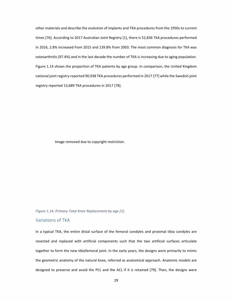
osteoarthritis (97.4%) and in the last decade the number of TKA is increasing due to aging population.

Figure 1.14 shows the proportion of TKA patients by age group. In comparison, the United Kingdom

national joint registry reported 90,938 TKA procedures performed in 2017 [77] while the Swedish joint

registry reported 13,689 TKA procedures in 2017 [78].

Figure 1.14. Primary Total Knee Replacement by age [1].

Variations of TKA

In a typical TKA, the entire distal surface of the femoral condyles and proximal tibia condyles are

resected and replaced with artificial components such that the two artificial surfaces articulate

together to form the new tibiofemoral joint. In the early years, the designs were primarily to mimic

the geometric anatomy of the natural knee, referred as anatomical approach. Anatomic models are

designed to preserve and avoid the PCL and the ACL if it is retained [79]. Then, the designs were


30

developed with philosophy to simplify the knee biomechanics by removing both cruciate ligaments,

referred as functional approach. Functional designs permitted “nonanatomical joint surface

geometries intended to maximize surface area and reduce polyethylene stress” [79]. Both approaches

resulted in some common features. However, as TKA advances, there are several different designs

aspects; the most major variations are outlined below.

Materials

Low friction is the one of the most important factors in selecting TKA bearing. Polyethylene has been

the primary bearing material due to its low friction property. Although modern hip arthroplasty are

now migrating to more advanced materials, such as ceramic‐on‐ceramic (CoC), this is less appropriate

for the knee. Unlike hip anatomy, which is spherical joint, knee has less conforming geometry as

discussed in knee anatomy section. In addition, the brittle nature of ceramics and the inability of

ceramic materials to withstand high‐impact tensile forces is of concern for TKA applications. The

femoral component is generally manufactured from cobalt‐chromium (Co‐Cr), providing high

strength, good biocompatibility and excellent corrosion resistance. The tibial articulating insert is a

medical grade ultra‐high molecular weight polyethylene (UHMWPE), e.g. GUR‐1020, GUR‐1050 or

GUR‐4150; however experiences with early designs demonstrated that the lower stiffness of

UHMWPE against cancellous bone could lead to failure [80], and it soon became standard for the tibial

polyethylene insert to be mounted in a metal tray (often Co‐Cr or titanium) for stiffer backing.

However, it was previously found that polyethylene free radicals produced in the radiation process

cause oxidative degradation which may threaten the long‐term stability of these devices [81, 82].

Polyethylene properties can be modified by sterilization by radiation and by exposition to the oxidative

environment; the effects are increase in density and elasticity of the materials itself. To counter these

problems, a range of refinements have been made to the production processes for UHMWPE (e.g.

gamma‐ray vacuum sterilisation is used to encourage polymer cross‐linking, which can further

enhance the wear performance while providing oxidative stability [83].

31

Cruciate Retaining Vs Posterior Stabilizer

While the anterior cruciate ligament is usually resected in TKA for surgery access, the posterior

cruciate ligament (PCL) may not be necessary resected as it helps stabilising the femur by preventing

anterior translation during knee flexion. This is only true as long as its function is preserved by careful

bone resection and adequately balancing the knee in flexion and extension. Prostheses designed for

retaining the PCL are called cruciate retaining (CR). However, sometimes, the PCL may be incompetent

due to injury or degeneration or surgeons may choose to sacrifice the PCL while performing TKA in

cases where flexion is tight, to prevent excessive stresses and wear of the polyethylene insert. The

prosthesis used for this scenario is called a posterior stabilizer (PS). This design substitutes the PCL

functions by means of a central cam on the femoral implant, which is pushed back by the central post

on the polyethylene insert (Figure 1.15). PS implants may provide better anteroposterior stability due

to cam‐to‐post mechanism. However, one of the potential draw backs with this design is tightness

(resulted in less ROM) in extension due to early contact between the cam and the post. Several studies

have investigated the differences in outcomes between these two designs finding no clinically

relevant differences between these two implants for clinical scores and gait [84‐86]. Additionally,

recent systematic review by Longo et al [87] compared clinical outcome scores, rate of complications

and ROM of PS and CR knees. They found literature reported PS knees tend to achieve a higher post‐

operative ROM while CR and PS knees have similar clinica outcomes.

32

Figure 1.15. (a) Cruciate retaining implant. (b) Posterior stabilizer implant. The cam‐to‐post substitute

the functions of PCL [79].

Variations of tibia bearing design

The use of metal backed insert is now widespread, and many designs now also introduce additional

degree of freedom between the tray and the polyethylene insert. One design concept is to use a

central peg, permitting only I‐E rotation between the tray and insert; i.e. a rotating platform (Figure

1.16, centre). Another concept is a slotted peg permitting both rotation and translation; i.e. mobile

bearings. These designs were introduced to prevent excessive stresses at articulating surfaces by

providing more conforming contact during motion (increase surface contact area and hence

decreasing contact stress) [88]. Nonetheless, fixed designs with no tibial bearing are still common.

Although theoretically rotating and mobile bearings offer advantages, currently these benefits do not

clearly translate to improved clinical results [89, 90].


33

Figure 1.16. Comparison of tibial bearing designs [73].

The Medial pivot design was introduced to address the issue of asymmetric tibiofemoral motion.

Conformity on the medial side was intended to provide reduced AP motion; less constraint on the

lateral side was intended to allow AP femoral translation. The asymmetry in the motion is provided by

the tibial and femoral components shape, which is a conforming socket on the medial side and an

arcuate surface around the centre point of the medial socket on the lateral side [91]. The design of

this prosthesis was finalized in the mid‐1990s, a time when wear of polyethylene was a major concern

and low contact stresses on the tibial insert were critically important. The ball‐and‐socket conformity

on the medial side resulted in large surface area and hence lower contact stresses. This attempt was

accepted in the interest of limiting detrimental effects of wear debris [92].

Single radius Vs Multi radius femoral component

It is known that in vivo kinematics after TKA is influenced by the design of the implant. Single‐radius

femoral component design was introduced in an attempt to more accurately reproduce the kinematics

of the natural knee. The design is based on the premise that there is only one knee functional‐

extension axis location [93, 94]. Unlike multi‐radius design, the femoral component rotates against

the tibial insert only in one radius in single‐radius prosthesis. Until now, there have been few clinical

reports about post‐operative function of the single‐radius design and they have been highly

controversial [95, 96]. Ostermeir [97] reported single‐radius design showed lower maximum extension

forces and Wang et al [98] reported that the single‐radius had better stability than the multi‐radius

one with respect to standing up from sitting position. On the contrary, two studies presented by


34

Stoddard et al [99] and Jenny et al [100] reported that improvement in using single‐radius design could

not be clinically demonstrated.

Figure 1.17. Single radius and dual radius femoral component [101].

Surgical Techniques

Patellar Resurfacing

The native patella may or may not be resurfaced in TKA. This is a continuous debate amongst

orthopaedic surgeons. Advocates for either side of the debate raise a number of valid points to

support their view on the matter. Orthopaedic surgeons who practice and support the notion to not

resurface the patella support their decision based on the number of risks that are associated with

resurfacing the patella. This includes patella component fracture, implant loosening and patella clunk

syndrome. However, non‐resurfacing of the patella is associated with a higher rate of anterior knee

pain and re‐operation [102‐105].

Extensive literature have compared the outcomes between resurfaced and un‐resurfaced patella in

TKA [106]. A meta‐analysis by Agrawal et al [107] reported that the existing literature shows that

patellar resurfacing can reduce the risk of reoperation with no improvement in knee function or


35

patient satisfaction compared to patients without patellar resurfacing [107]. Despite of the

controversy, the use of patellar resurfacing is continuously increasing, as shown in Figure 1.18.

Figure 1.18. Primary TKR by patella usage [1].

When the patella is resurfaced, the bone is resected with the aim to restore the patella’s original

thickness. In general, the patella component is all‐polyethylene. The articular surface geometries of

the patella component can be classified into five basic shapes: [108] convex or dome shaped; modified

dome shaped; anatomically shaped; cylindrical or saddle shaped; mobile bearing.


36

Figure 1.19. Variations of patella button design available in the market [108].

Navigated TKA

It is well known that correct alignment of the components is one of the most important factors to a

successful TKA; it is believed a well aligned TKA is likely to function well. Traditionally, intraoperative

knee alignment has been achieved by instrumentation with intramedullary and extramedullary

alignment rods and more recently using patient specific positioning guides which uses preoperative

MRI or CT to design custom shape‐fitting jigs [109]. Mechanical instrumentation can be fiddly which

may lead to inconsistent or inaccuracy results. Recently, computer navigation systems have gained

substantial popularity in TKA industry (as shown in AOANJR data in Figure 1.20). Their aim is to provide

more accurate implantation by digital mapping based on standard anatomical landmarks and intra‐

operative assessments [110]. There are two different types of imaging systems, all of which need

intraoperative registration of anatomical landmarks [111]. Image‐based systems need the collection

of morphological information by pre‐operative computed tomography (CT) or intra‐operative

fluoroscopy. Imageless systems, which use a virtual model supplemented by registration data, have

overcome concerns about exposure to radiation [112].


37

A number of studies [110, 113, 114] have suggested that there is improved alignment when navigation

is used. In a meta‐analysis, Mason et al [115] compared mechanical axis alignment between computer

assisted and conventional knee replacements, and reported malalignment of greater than three

degrees in 9% of computer assisted knee versus 31.8% of conventional TKAs. Despite this,

contradictory evidence does exist with other recent meta‐analyses arriving at markedly different

conclusions. Bauwens et al [112] and Calliess et al [116] concluded that despite of few advantages

that computer assisted TKA provides over conventional surgery on the basis of radiographic end

points, its clinical benefits are unclear and remain to be defined on a larger scale. Barrett et al [117],

in a multi‐centre prospective randomized trial, reported a significant improvement in coronal tibial

alignment following computer navigation, but this was associated with a significant increase in

operative time.

Figure 1.20. Primary TKR by computer navigation[1].

Soft Tissue Balancing

In addition to correct limb alignment to achieve successful TKA, the knee need to be balanced the

knee in both extension and flexion [118]. A balanced extension gap can be achieved by either aiming


38

for appropriate bone cuts or soft tissue release. Bone cuts will be attempted first. Only after these, if

necessary, should a surgeon look at making soft tissue releases. Example of soft tissue release, lateral

structures are released to balance a valgus preoperative deformity and medial structures are released

to balance a varus knee. Femoral component rotation is essential in achieving symmetry flexion gap

[119]. Improper femoral component rotation may result in asymmetric flexion gap which may lead to

patellofemoral instability [120], anterior knee pain, arthrofibrosis, and patient discomfort due to

instability on the knee [121‐123].

There are two surgical approaches in achieving good components alignment and a balanced knee;

measured resection and gap balancing. These approaches employ different techniques to determine

femoral component rotation and ligament balancing.

1. Measured resection (MR): aims to resect an amount of bone equal in thickness to the

prosthesis to be implanted. Distal femoral resection is angled in respect to the femoral shaft [124].

Femoral component rotation should be parallel to one these three bony landmarks; the epicondylar

axis, posterior condylar axis, or the AP trochlear axis (Whiteside’s line) [125‐127]. The anteroposterior

position, or size, of the femoral component can be determined with either anterior or posterior

referencing [128, 129]. The tibial resection is done independently, perpendicular to the long axis of

the tibia in the coronal plane. Ligament balancing is done once the trial components are in‐situ.

2. Gap balancing (GB): distal femoral and proximal tibial resections are performed first. The

femoral component rotation is positioned parallel to the resected proximal tibia with each collateral

ligament equally tensioned to obtain a rectangular flexion and extension gap [119, 130, 131]

Few studies have reported that the determination of bony landmarks in MR technique varies and thus

suggest GB may offer superior reliability compared to MR method [119, 123]. The variability of

determining the bony landmarks may result in higher risk of femoral component malorientation [125].

39

Dennis et al [126] compared the stability of 40 MR TKAs and 20 GB TKAs and found that the incidence

and magnitude of femoral condylar lift‐off was much lower in GB than MR TKAs. Nevertheless, despite

of the bony landmarks variability, MR showed better joint line preservation by avoiding excessive

medial structures release [132].

On the other hand, a precise proximal tibial resection is critical when using a gap resection technique

[119]. The tibial cut is utilized to create the flexion space at 90°. Consequently, any varus or valgus

malalignment will result in increased internal rotation of the femoral component when the femoral

component is placed parallel to the resected proximal tibia [131]. Additionally, it is critical in GB to

accurately control the distraction forces while balancing in both extension and flexion.

Nagai et al [133] in their findings indicated that due to the lateral compartment stiffness being much

lower than the medial compartment, the lateral compartment gap tends to be larger than the medial

compartment gap as the joint gap distraction force increases. This suggests that if the surgeon only

applies a low joint distraction force, the varus ligament balance is low and therefore the rotation of

femoral posterior condyle resection is small. Another challenge in GB method is to achieve stability in

mid‐flexion. A recent study demonstrated that a significant proportion (36%) of TKAs showed

midflexion laxity even when rectangular extension and 90° flexion gaps were achieved [134]. The

flexion and extension gaps can be measured with ruler, lamina spreaders or tensioner. In addition, it

is also critical to pay attention to patellofemoral joint while balancing the knee. Excessive femoral

component rotation may alter patellar tilt angles [135] and kinematics [123, 136].

Failure of TKA – what are the causes?

Assuming the initial arthroplasty surgery is successful, there are still many risks of failure post‐

operatively. Interestingly in contemporary TKA, failure is no longer only categorized as the need for

revision, but also a measure of patient satisfaction. For example, a patient may have limited

functionality even though they do not require a revision surgery. This will be discussed further in the

next section. Table 1.4 represents the causes of failure of large TKA revision reported in literature

40

[137, 138] and joint registry report [1, 139] . Sharkey et al., differentiated between early and late

complications. Whereas infections are typical early complications, aseptic loosening and wear occur

generally late after TKA implantation. Note that these factors are not independent or exclusive (e.g.

wear‐induced osteolysis may lead to loosening or increase the risk of direct mechanical failure of the

component). Some of these factors are unrelated to mechanical environment and others depend

strongly on joint mechanics (indicated in bold). In a recent follow up study by Sharkey et al., [140]

infection was still the most common reason for early revision but polyethylene wear was no longer

the primary reason for late revision. Aseptic loosening was the most common reason for late revision.

Table 1.4. Causes of TKA failure

causes of failure %a

%b %c %d

%e

early late early late

aseptic loosening 25 17 33 25.9 38.7 23 51.4

wear/osteolysis 15 11 44 3.7 9.6 5 10

instability 14 ‐ ‐ 7.3 17.6 10 10

infection 11 25 10 22.5 5.8 37.6 21.9

mechanical failure 7 ‐ ‐ 1.5 1.3 ‐ ‐

periprosthetic fracture 4.5 2 3 2.8 4.0 8 8

pain 2 ‐ ‐ 8.6 16.9 ‐ ‐

dislocation 2 ‐ ‐ ‐ 4.2 ‐ ‐

arthrofibrosis ‐ 18 20 3.5 5.9 10 5

malalignment ‐ 11 12 2.2 7.9 3 5

extensor mechanism deficiency/patellar complications

‐ 10 2 16 ‐ 2 1

avascular necrosis patella ‐ 4 4 ‐ ‐ ‐ ‐

Incorrect sizing ‐ ‐ ‐ 1.2 ‐ ‐ ‐

other ‐ ‐ ‐ 4.9 21.1 ‐ ‐ a Gioe et al [137] b Sharkey et al ‐ 2002 [138] c 2017 Australian Joint Registry [1] d 2018 National Joint Registry for England, Wales, Northern Island and the Isle of Man Joint Registry [139] e Sharkey et al – 2012 [140]

41

Outcomes of TKA

TKA is considered as one of the most successful operations when measured against longevity, the

cumulative revision rate at 16 years is 8.0% or survivorship rate of 92.0% [1] (Figure 1.21). However,

implant survival as an outcome (i.e. implant not removed from the patient’s body) does not indicate

patient is satisfied with the results from the surgery, as a patient may still be in pain or suffer from

lack of function. This was highlighted in recent studies, where 15 to 20% of patient’s were dissatisfied

after surgery, including reports of persistent residual pain [141‐147]. This discrepancy between

successful survival outcomes and patient dissatisfaction supports the principle that a single discrete

success/failure metric is not sufficient to define the outcome of TKA. At the core of the issue is a

definitional difference between what constitutes a successful surgery, and the failure to fully align

patient expectations with the reality of their likely surgical outcome.

In 2009, Bourne and colleagues carried out a study to determine the reasons of dissatisfaction after

TKA. They found that when patients were most dissatisfied when their expectations were not met one

year after surgery [143]. This notion is supported by the work of Mahomed et al., [148] who found

that patients expectations could be low (i.e., expected to have no pain after recovery from surgery)

and high (expected to have no functional limitations) [148].

42

Figure 1.21. Cumulative percent revision of primary TKR [1].

PROMS as outcome measurement

Revision rate is a common outcome measure in TKA [149‐152] and even considered to be the gold

standard for survival analyses of orthopaedic implants [153]. However, the reliability of using revision

rate as an outcome measure has been questioned [150, 153].

In addition to revision rate, patient‐reported outcome measures (PROMs), are subjective scores used

as additional assessment to gauge the surgery’s success from patient’s perspective (clinical outcome)

[154‐157]. Oxford Knee Score (OKS) [156, 158‐163], Knee injury and Osteoarthritis Outcome Score

(KOOS) [158, 164‐172], Western Ontario and McMaster Osteoarthritis index (WOMAC) [173, 174],

Knee Society Score (KSS) [158, 175‐178] are few most common PROMs questionaries. As PROMS are

subjective scores, they tend to have high variability and may have low repeatability.


43

While there is a trend for PROMS to increase from pre‐op to post‐op, studies generally show that TKA

patients still experience some pain and/or loss of function post‐operatively. For example, Bourne et

al [2] and others [141, 154, 179] have shown about 20% of patients are dissatisfied following TKA.

This suggests that pain and function, rather than revision rate results in a much a higher failure rate,

and probably provide a better outcome measure for success. There are also situations when revision

rates mask poor outcomes, such as in poor functional outcomes which do not warrant revision, but

may impede participation (i.e. restricted knee flexion range) [180].

Furthermore, pre‐operative patient selection might mask the true effectiveness of the treatment. For

example, patients who have higher expectations (e.g. younger patients) tend to show greater

dissatisfaction [181‐183]. One important conundrum of TKA outcomes is that patients with high pre‐

operative functional status are associated with worse subjective scores following TKA [182] and at the

same time, patients with worse pre‐operative functional status also exhibit the most dramatic

improvement following TKA [181, 182]. This apparent contradiction highlights the fact that not only

post‐operative subjective scores values are important, but also the amount of improvement following

TKA, as suggested by Losina et al [184]. In other words, an objective outcome for TKA requires to

measure the improvement of pain and function considering the difference between a preoperative

baseline and post‐operative outcome measurements. Regardless of the increasing number of studies

assessing outcomes of TKA [154, 185‐191] , a consensus has yet to be reached on whether to define

success based on the degree of improvement from pre‐operative status (the journey), or based on the

level of pain or functional status achieved at a specific point in time (the destination) [184].

Nevertheless, the literature has consistently shown about 20% of TKA patients are dissatisfied. In 2017

itself, there were an additional 52,836 TKAs performed in Australia from the previous year. Therefore,

with the increasing number of TKA performed each year, it is critical to gain better understanding of

the different approaches towards the procedure, how they are or are not addressing individual patient

needs and engineer appropriate solutions to help towards improvement of patient’s quality of life.

44

Component alignment as outcome measurement

It is of general acceptance that TKA procedures aim to have an overall lower limb alignment in coronal

plane is 0° ± 3° [10, 112, 160, 192], so that the limb is aligned with the mechanical axis, which is

believed to promote implant durability [193]. This target is described as mechanical alignment (MA).

Misaligned implants may lead to wear and/or loosening of one or both components, or patella

instability resulting in early failure and revision surgery [194‐196]. Numerous studies have correlated

the survivorship and post‐operative function improvement with coronal plane limb alignment [157,

170, 177, 197‐201] but the relationship is not well understood.

Recently, the philosophy of kinematic alignment (KA) or natural alignment has emerged as an

alternative to restore normal knee motion and function [146, 175, 192, 196, 202]. Kinematic alignment

is considered as restoration approach which aimed to align the angle and level of the distal joint line

of the femoral component, posterior joint line of the femoral component, and joint line of the tibial

component to those of the normal knee [144, 192, 202, 203]. This approach will achieve different

component alignment for different patients, somewhat a step towards personalisation of component

alignment [203] .

The clinical outcomes of kinematic alignment are still unclear although few studies have reported

patients are doing well when short term functional outcomes (e.g. Oxford Knee Scores, WOMAC,

ROM, Knee Society Score, KOOS) were measured at one year [170] and 2 years and with some

studies showing improved outcomes using this approach compared with the traditional MA [204, 205].

Nevertheless, Despite the good intention of restoring the knee to the pre‐disease state, there is on‐

going debate whether restoration (KA) or reconstruction (MA) will yield a better patient functional

outcome [144, 196]. Concerns had been expressed in few studies that full restoration of the knee joint

may result in extreme component alignment and may lead to early implant failure due to imbalance

loading on the tibia insert compartments [202, 206‐208]. However, studies have determined no

difference in the risk of early failure between MA and KA [175] stating that the concern that kinematic

45

alignment compromises function and places the components at a high risk for catastrophic failure is

unfounded [202]. Figure 1.22 below illustrates component alignment difference between MA and KA

with respect to femur and tibia mechanical axis.

Other studies have recently looked at the restricted Kinematic Alignment (rKA) [146, 192], a more

conservative approach. rKA is proposed when the native anatomy is considered to have an extreme

deformity to the point when kinematic alignment is applied, it would impact function recovery with

potential residual pain. This approach is a compromise between Mechanical and Kinematical

alignment where the suggested alignment of the components will be placed within a value between

the native anatomy and the mechanical alignment threshold.

Component alignment has been shown to impact postoperative PROMS. However, reported studies

have not yet shown a consensus on which alignment philosophies yield better clinical outcomes. This

would suggest that a single alignment philosophy may not be applicable as an optimal target for all

patients.

Relationships between component alignment and joint dynamics behaviour have been previously

shown to exist. Planckaert et al studied correlation of knee kinematics to dynamic behaviour of the

knee and pain after TKA. [200]. Their findings showed dynamic knee flexion contractures, increased Q

angle, patellar lateralization and internal rotation of the combined components, all of which are

characteristics that tend to increase patellofemoral forces and could be the cause of anterior knee

pain. Similarly, study by Barrack et al [209] indicated that patients with anterior knee pain had

significant internal rotation at the tibial component and in the combined component of approximately

6 degrees and 4.7 degrees respectively.

46

Figure 1.22. Illustration of mechanical and kinematic aligned components. Left is mechanical

alignment where the components are aligned to bone mechanical axis. Right is kinematic alignment

where components are aligned to bone’s joint line.

Other examples include studies from University of Denver [210‐213]. They have been studying the

patellofemoral joint and the factors that affect its biomechanics. They investigated the resection

thickness of patella on kinematics and quadriceps efficiency [210] and found that at lower flexion

angles, there was a small increase in quadriceps force with thinner composite patellar thickness. In a

different study, Keshmiri and colleagues [214] found that femur and tibia sagittal alignments had a

significant influence on patellar kinematics but the rotational alignment did not have a significant

effect.

Above examples show that joint dynamics may be more relevant to clinical outcomes than component

placement alone. However, studies have not shown identifiable reproducible relationships with joint

Mechanical alignment Kinematic alignment

47

dynamics clinical outcomes, indicating that clinical outcome of TKA is a product of complex

interactions between surgical and patient factors. Surgical factors can be attributed to interactions

between the component design, component alignment, and patient specific anatomic characteristics.

Joint dynamics can be measured with different techniques. Gait labs and video fluoroscopy techniques

are a means of capturing patient’s movement functionally. However, facilities for these techniques

are not widely available, which may limit the scalability of its use in clinical setting. Mechanical

simulator is an alternate technique but is limited in its capture of patient specific factors. Furthermore,

mechanical simulator can only be done in cadaver specimen, which limits the applicability to study

individual patients. Validated computational modelling is a more scalable alternative technique and

allow to joint dynamics to be evaluated under various conditions and surgical factors. Computer

simulations have been used to optimize implant designs [215, 216] and are increasingly used to study

dynamic relationships [217, 218].

Computational Modelling

Computational models are used to describe, explain and predict real world events, such as weather,

economy, social interactions, demographics, drug effects, and anatomical and physiological

mechanisms in animals and humans. The complexity of the model will depend on the question

researchers and scientists are attempting to answer, the assumptions made and the population under

study. Simple models can be scalable and extrapolated to a wide population from few real data

measurements and general parameters; more complex models the introduction of more parameters

and more measurements as different sections of the population will present a considerable variation

in parameters.

Computational modelling in biomechanics context can be categorised into two main groups based on

the level of complexity, Rigid Body Modelling (RBM) and Finite Element Modelling (FEM). RBM

simplifies the analysis with the assumption that the body segments under analysis are rigid, they do

48

not deform under the action of applied forces. These models are used to study the dynamics of human

motion by calculating the displacements of each body segment with respect of each other and the

overall motion on a global reference system. Unlike RBM, FEM allows for structures to be modelled as

deformable bodies, by applying fundamental physical equations discretised across small spatial and/or

temporal intervals. As these intervals become smaller, the approximation becomes better up to a

certain limit, but computational effort also increases as the number of separate discretised equations

increases. FEM models are often static or quasi‐static due to the high computational effort. In other

words, RBM is mainly used to study for overall kinematics ad kinetic analyses, whereas FEM is used

for studies aimed to determine analysis of contact forces, stresses and deformation between

segments.

Computational models of human motion can be separated further into two categories: inverse

dynamics and forward dynamics. Both of these methods are currently used by those who simulate

human motion [219], and both are able to provide estimations of muscle forces that are otherwise

impossible to measure. The critical differences between these two models outlined in the following

sections.

Inverse and forward dynamics

Inverse dynamic modelling is a computationally inexpensive technique, and can provide researchers

with accurate and meaningful data, such as muscle forces and joint moments. When using inverse

dynamics, the position, velocity, and acceleration of a segment are used to estimate muscle forces

(Figure 1.23). These calculations rely on the measurement of segmental kinematics and kinetics

calculated using 3D motion capture systems and force plates within an instrumented gait analysis

laboratory. The inverse dynamics method requires calculation of moments about each joint from

measured kinematics and ground reaction forces and muscle forces are estimated by solving a static

optimization problem at each instant during the movement.

49

Figure 1.23. A block diagram of the inverse dynamics technique [220]. External forces, position, velocity and acceleration of a segment are used as inputs to solve for internal joint forces. Then the individual muscle and ligament forces are optimized based on the calculated internal joint forces.

On the other hand, forward dynamic modelling is more computationally expensive, as simulations are

created by the numerical integration of differential equations describing the motion of body segments

(Figure 1.24). Unlike inverse dynamics, which determines muscle forces from measured motions and

external forces, forward simulations rely upon muscle forces as input to produce motions. Model

parameters, such as muscular, ligamentous force, initial joint angels and velocity can be optimized at

each time step in an effort to replicate the experimental kinematics as closely as possible.

Figure 1.24. A block diagram of the forward dynamics technique [220]. Internal forces and external forces are used as inputs to produce motions of the model. Forward dynamics modelling is more computational expensive than inverse dynamics as the model needs to integrate numerous of differential equations to produce motions.

The application of computational models to knee joint

Computational models for the analysis of human movement have focused on analysing the knee

complex, which is comprised of two joints, namely tibiofemoral and patellofemoral. The aim of these

models has been to understand native movement, common injuries, the development and treatment

50

of osteoarthritis (OA) [216, 221‐225]. These methods have been used to analyse contact behaviours,

biomechanical properties of articular cartilage [226‐228], ligament reconstruction [222, 229],

meniscectomy [230, 231], and knee replacement [217, 218, 224, 232‐236].

One of the earliest works in computational modelling of the knee was carried out by Blankevoort and

colleagues in the early 1990s [237]. In this work, they analysed the kinematics of the knee joint during

passive motion using a 3D mathematical model with ligament insertions and geometrical data

obtained from experimental study. Their study is the first to compare the effect of rigid contact and

deformable contact. They showed there was small difference between rigid and deformable contact

kinematics for passive motion. In their model, ligaments were described with two or more spring

elements representing ligament fiber bundles, which were assumed to be non‐linear and the

mechanical characteristics of the ligaments were derived from previous mechanical testing [238]. Also

in 1990s, Abdel‐Rahman et al [68] developed a 3D model to study the dynamic response of the knee

joint. Their work focused on mathematical equations contact formulation. Similar to Blankevoort

studies, they used 1D nonlinear spring elements to represent knee ligaments. There were other groups

developed computational model to study the passive kinematics in 2D [239, 240]. During this period,

most studies focused on algebraic equations describing the 3D dynamic behaviour of the joint [241]

and as such no computational model that includes both tibio‐femoral and patello‐femoral joints has

yet been developed [241].

In early 2000, Guess et al [242] developed a 3D computational model incorporating both tibio‐femoral

and patello‐femoral joint to replicate the behaviour of a dynamic knee simulator. Their model was

developed with a multibody dynamics solution software created by ADAMS (MSC Software

Corporation; Santa Ana, CA). In this study, joint contact is modelled as a non‐linear spring damper

system. The goal was to develop and verify a 3D model of a knee simulator so that knee loads, and

kinematics could be used as input to generate muscular force profiles for an identical experimental

knee simulator.

51

A simplified rigid body model called KneeSim was created by LifeModeler, Inc, San Clemente,

California in 2000s. This model also uses ADAMS as the underlying mathematical solver. The model

consists of tibio‐femoral and patella‐femoral joints. The model replicates a deep knee bend simulator,

Oxford Knee Rig [243]. The soft tissue were modelled as non‐linear springs, subject specific [244] or

scaled attachment sites [245, 246] can be used. This model has been used in literature by different

research groups to analyse post‐operative TKA kinematics or as pre‐clinical tool to assess different

implant system performance. Mihalko [247] studied how the kinematics vary with different

combinations implant positioning in the transverse plane of both the femoral and tibial components.

Mizu‐uchi et al [244] compared the post‐operative flexion range of TKA with clinical measurement and

the simulation predict the flexion angles to be within 2°. Okamoto et al [248] studied the effect of tibia

posterior slope on PS insert using the same model and Nakamura et al [249] investigated the effect of

superior‐inferior position of the patella component to anterior knee pain reported by patient.

Further historical use of computational model was discussed by Rullkoetter et al [216] and Walker et

al [215]. They described how computational models had been used in pre‐clinical environment as tool

to study implant design features. They explained how this approach can be used to minimize the

development cycle by reducing the time and expenditure in testing physical prototypes and allowing

for the evaluation of multiple design concepts, thereby improving the clinical performance of implants

[216]. In their publication, Rullkoetter exemplifies the use of computational models to improve the

stability and mobility of knee implants by considering laxity assessment, compressive loads and muscle

force requirements.

Soft tissue representation, particularly ligament in knee computational model is important. They have

a large effect on knee joint kinematics and biomechanics. Galbusera et al [67] showed the wide range

of element types and material models used in computer models. Similarly, in Beidokhti et al [66]

investigated the effect of ligament modelling strategy on the predictive capability of computer models

of the human knee joint. They reported that although 3D representation of ligament structures

52

resulted in a more accurate outcome variable comparison, however ligament represented with spring

models provides a faster option with acceptable outcome when joint kinematics is the main interest.

Baldwin et al [217] developed and verified a knee model based on experiment data from Kansas Knee

Simulator (KKS). In the study, each of the cadaver specimen was subjected to laxity‐test and dynamic

activities. Experimental laxity‐test data were used to optimize the mechanical properties of

tibiofemoral ligament structures on a specimen‐specific basis. Each specimen is then subsequently

analysed in a computational model that represent KKS dynamic activities. They reported they were

able to achieve good agreement in trends and magnitudes between model predictions and

experimental kinematics. Other researchers followed a similar approach to develop complex models

to estimate patient specific soft tissue properties using data from testing laxity experimentally [250‐

253]. Although these models were able to derive subject specific ligament parameters, they required

many hours of computational time to produce results, and hence limit the practicality to be used in

clinical setting.

In contrast to using experimental data, some models rely on scaled parameters based on generic

anatomy [254, 255], generic assumptions of soft and bony tissue morphological and physiological

characteristics [245, 256, 257], or focused on isolated tibiofemoral joint [258‐260]. Simplifications

made in these models reduces computing power and can still show relevance in simulation outputs,

particularly joint kinematics, as reported by [66]. An example of the use of a simplified model reported

in literature. Ishikawa et al assessed patellofemoral and tibiofemoral kinematics behaviour of a

mechanically and a kinematically aligned implants using rigid body modelling. Further, they studied

the patellofemoral and tibiofemoral contact stresses using finite element analysis. Their model

included assumptions on the characteristics of tibiofemoral and patellofemoral contact; tissue

characteristics of LCL, MCL, PCL; elements of the knee capsule; and anatomical and physiological

characteristics of the quadriceps muscle and tendon, patellar tendon, and hamstring muscles. In this

approach, the LCL was modelled as a single fiber bundle; and the MCL as anterior and posterior

53

bundles; ligaments were modelled as nonlinear springs; and the PCL was defined as being composed

of two bundles. Regardless of the assumed parameters, they were able to demonstrated that although

kinematically aligned implants produced near normal knee motion, it increases contact stress after

TKA when compared to mechanically aligned components [261].

Since the initial development phase in 1990s, there has been considerable improvement in the

complexity, accuracy and functionality of the models. Geometries and mesh used in model have

moved from idealised 2D to scaled anatomical based model and subject specific 3D model. The use of

computational models has expanded from passive motions to dynamic motions. Efforts have been

made to optimize subject specific ligament properties using experimental method. However, many of

the developed computational model have not been validated. Furthermore, computational model

used regularly as part of pre‐operative surgical planning has yet been developed. The closest rigid

body model that have been used by few researchers group is KneeSim developed by Lifemodeller.

Even though subject specific geometry can be used, its application in pre‐operative setting is not

optimised. Outcome of TKA depends on both surgical and patient factors which can be studied using

computational model. Therefore, there is a need to develop a validated low‐cost computational model

that is practical to be used regularly for TKA surgical planning.

Summary

Total knee replacement is a solution to end‐stage osteoarthritis. Although TKA shows good

survivorship, patient dissatisfaction is one of the major current concerns post‐surgery. Improving

patient quality of life is of paramount importance. Joint dynamics have shown to have relationship to

clinical outcomes which affects patient satisfaction. Joint dynamics is a product of complex

interactions between surgical and patient factors. Computational modelling is a scalable technique

compared to other functional techniques and allow the study of both surgical and patient factors

impact on joint dynamics following TKA. The computational model developed however need able to

54

be used practically in clinical setting, in other words low cost computational model in order to realise

the use of such tool to optimise joint dynamics as part of TKA surgical planning.

Computational models can be highly complex depending on the research or clinical application for

which they are developed. For instance, patient specific models tend to be highly complex and require

measurements that would include, 3D motion analysis (kinematics and kinetics), electromyography.

Nevertheless, acquiring such amount of information is time consuming, impractical and expensive as

it would require several patient appointments, the use of extremely specialized equipment and the

contribution of a multidisciplinary team for capturing, processing and interpreting all data.

On the other hand, a simple, generic model, scalable using crude anthropometric measurements and

generalized anatomic relationships resulting in poor representation of an individual patient limiting

the clinical significance of the model. Thus, a trade‐off between complexity and clinical applicability

must be sought. A model that is too complex require more specific inputs and longer time to simulate

which in return require more data that potentially need to be collected clinically. On the other hand,

model that is too simple, accuracy on clinical relevance will be reduced. The relationship between

complexity and practicability of a computational model is represented graphically on Figure 1.25.

Ideally, for clinical applications, a computational model is on the top right quadrant. However, with

increasing complexity, computational and economical cost will increase.

Thus, a balance needs to be found in between the right quadrants. Another important aspect is the

applicability of the developed computational model. All models have inherent inaccuracy within them,

even with the most complex model. But a model would still be useful if it provides information that

otherwise clinician won’t have and can be related to clinical observations.

55

Figure 1.25. Complexity vs practicality matrix for computational model

56

Chapter 2

Variability in Static Alignment and Kinematics for Kinematically Aligned TKA

This chapter was published in The Knee Journal

Theodore W, Twiggs J, Kolos E, Roe J, Fritsch B, Dickison D, Liu D, Salmon L, Miles B, Howell S,

"Variability in static alignment and kinematics for kinematically aligned TKA," (in eng), Knee, vol. 24,

no. 4, pp. 733‐744, Aug 2017.

This chapter presents the development of a simplified computational model of the knee replicating a


kinematically aligned components.

57

Introduction

Total knee arthroplasty (TKA) is an established procedure for improving pain and restoring a significant

degree of function, especially for low‐demand activities of daily living. However, an understanding of

optimal alignment and patient specific kinematics are needed to restore knee motion closer to normal,

allowing performance of physically demanding activities that more active patients consider important

[262‐264].

The philosophy of mechanical alignment of the implant after TKA has traditionally been done to

preserve longevity of the implant and enhance post‐operative knee function [177, 265, 266]. However,

studies have shown that although a mechanically aligned TKA improves the patient’s function, 20% to

25% of patients remain dissatisfied [2, 142]. In addition, recent data has challenged the importance of

post‐operative mechanical alignment in TKA. Paratte et al [267] in a study reviewing 398 TKAs,

demonstrated no improvement in the fifteen year implant survival rate in patients within and outside

of a post‐operative mechanical alignment 0° ± 3°.

Recently, kinematic alignment has been proposed by Howell et al [263, 268, 269] as an alternative to

restore normal knee motion and function. Kinematic alignment references the femoral transcylindrical

axis, believed to be the flexion extension axis of the knee. The aim is to align the angle and level of the

distal joint line of the femoral component, posterior joint line of the femoral component, and joint

line of the tibial component to those of the normal knee [269].

Kinematically aligned TKA has been performed since 2006 however unanswered issues continue

regarding patient outcomes, survivorship, surgical technique and use of specialised surgical guides

[202, 205, 270, 271]. One factor could be that there is no literature reported on long term clinical

outcome of kinematically aligned TKA yet. So far, studies up to 4 years are available and they reported

similar findings. A randomized controlled study demonstrated kinematically aligned TKA resulted in

better pain relief, post‐operative function and range of motion than mechanically aligned TKA in 88

58

patients (88 knees) after 2 years [205]. Other studies emphasized higher function as assessed using

the Oxford Knee Score and WOMACTM score on 198 patients (214 knees) after 4 years [202]; on 101

patients (101 knees) with kinematic alignment after 6 months [271]. However, one small series

emphasized the potential for malalignment using the OtisKnee system, which places implants at

higher risk of early failure [270].

The optimal targets for alignment in TKA remain unclear, and indeed a single philosophy may not be

applicable to an optimal outcome in all patients. Computer simulations are powerful tools that can

provide insight into how different alignments influence post‐operative outcomes for TKA patients. It

allows control of component alignment for the same subject in ways not possible with in‐vivo studies.

With imaging data, computer simulations are also able to include patient variations into the analysis

[245, 247, 257, 272]. Previous studies with computational models have shown comparable kinematic

and forces to those measured experimentally or with in‐vivo fluoroscopy [217, 273‐275].

Ishikawa et al [261] were able to analyse kinematic alignment for TKA using a computational knee

simulation. Their study suggests kinematically aligned TKA produces near‐normal knee kinematics and

may provide better clinical results than mechanically aligned TKA. However, only a single model was

used in the study and the kinematic alignment for that single model was defined with the clinical

average and therefore its conclusions were limited.

The aim of our study was to compare the alignment and motion of kinematically and mechanically

aligned TKAs with a computational knee simulation using pre‐operative CT scans from a series of 20

patients undergoing TKA. Validated computer simulation of both kinematic and mechanical alignment

was performed for each subject. Measures of tibio‐femoral translation, tibio‐femoral rotation, patellar

tilt and patellar shift were taken and compared between kinematic and mechanically aligned knees.

Materials and Methods

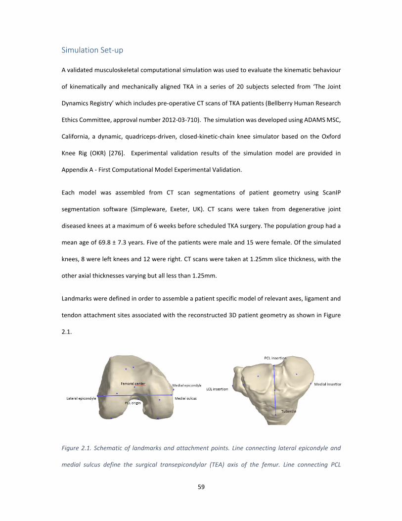
59

Simulation Set‐up

A validated musculoskeletal computational simulation was used to evaluate the kinematic behaviour

of kinematically and mechanically aligned TKA in a series of 20 subjects selected from ‘The Joint

Dynamics Registry’ which includes pre‐operative CT scans of TKA patients (Bellberry Human Research

Ethics Committee, approval number 2012‐03‐710). The simulation was developed using ADAMS MSC,

California, a dynamic, quadriceps‐driven, closed‐kinetic‐chain knee simulator based on the Oxford

Knee Rig (OKR) [276]. Experimental validation results of the simulation model are provided in

Appendix A ‐ First Computational Model Experimental Validation.

Each model was assembled from CT scan segmentations of patient geometry using ScanIP

segmentation software (Simpleware, Exeter, UK). CT scans were taken from degenerative joint

diseased knees at a maximum of 6 weeks before scheduled TKA surgery. The population group had a

mean age of 69.8 ± 7.3 years. Five of the patients were male and 15 were female. Of the simulated

knees, 8 were left knees and 12 were right. CT scans were taken at 1.25mm slice thickness, with the

other axial thicknesses varying but all less than 1.25mm.

Landmarks were defined in order to assemble a patient specific model of relevant axes, ligament and

tendon attachment sites associated with the reconstructed 3D patient geometry as shown in Figure

2.1.

Figure 2.1. Schematic of landmarks and attachment points. Line connecting lateral epicondyle and

medial sulcus define the surgical transepicondylar (TEA) axis of the femur. Line connecting PCL

60

insertion and tubercle define the tibia anterior‐posterior (AP) axis which then projected onto a plane

perpendicular to the mechanical axis to be used as AP rotational axis as defined by Insall [277].

The model includes the lateral collateral ligament (LCL), medial collateral ligament (MCL), posterior

cruciate ligament (PCL), patella tendon, quadriceps tendon and posterior knee capsule. The LCL was

considered to be a single fibre bundle and the MCL was considered to consist of anterior and posterior

bundles. Likewise the PCL was modelled as an anterior and posterior bundle and was differentiated

into anterior and posterior bundles by translation determined from experimental validation.

The femoral attachment points for the LCL and MCL were defined as the epicondylar prominences.

The fibular LCL attachment was defined as attaching to the lateral‐proximal centre of the fibular head.

The tibial attachment points of the MCL bundles were modelled as attaching at the superior‐inferior

level of the peak medial prominence of the medial edge of the tibia distal to the plateau, with anterior‐

posterior position at the peak medial projection. The PCL’s attachment on the femur was modelled as

residing midway distally down the posterior intercondylar fossa when viewed from a posterior

perspective, with the centre of attachment of the band placed one third of the width of the

intercondylar fossa from the lateral edge of the medial condyle. Its tibial attachment was defined as

the centre of the posterior intercondylar fossa.

The mechanical axis of the femur was defined as the line between the centre of the intercondylar

notch to the centre of the femoral head, while the tibial mechanical axis was defined as the midpoint

of the medial and lateral malleoli at the ankle to the midpoint of a line joining PCL insertion point and

medial third of the tibial tubercle. The PCL insertion point and medial third of the tibial tubercle were

then projected onto a plane perpendicular to the mechanical axis in order to define the tibial anterior‐

posterior (AP) rotational axis, as defined by Insall [277]. The surgical transepicondylar axis (the neutral

femoral rotational axis) was defined by the lateral epicondylar point and the sulcus of the medial

epicondyle.

61

Ligaments were modelled as point to point non‐linear springs, shown in Equation 2.1 [257].

Equation 2.1 Axial force sustain by ligament

Where f is the axial force sustained by the ligament, k is a stiffness parameter, ε is the strain and 2εl is

the threshold strain which indicates the change from the toe to the linear regions. The threshold strain

used is adapted from literature [68]. The stiffness coefficients of the PCL, LCL and MCL were initially

adapted from previous studies [68, 237, 257, 278]. Ligament stiffness’s were then adjusted based on

experimental validation performed with a cadaver study. Initial pre‐strain in each ligament in

extension was assumed to match values reported previously in literature [68]. The patella tendon and

quadriceps tendon were modelled as wrap‐able segmented links with femoral component contact to

allow for wrapping about the anterior femoral component in flexion.

The Simulation

The simulation model simulated a closed‐kinetic‐chain knee extension based on the OKR. All

components were modelled as rigid bodies with kinematic and compliant constraints, using a penalty‐

based contact between components. The model initialised in extension and then the ankle joint was

held rigid, which had three degrees of rotational freedom but was constrained in translation. The hip

joint was positioned above the ankle joint and was allowed freedom in flexion‐extension and varus‐

valgus, with the vertical motion guided by the axis drawn from the ankle‐joint to the hip joint.

In the flexion cycle of the simulation, a negligible force was applied through the extensor mechanism

to model soft tissue tension. Following the flexion cycle, the extensor mechanism was activated, using

a force applied through the quadriceps tendon to drive the knee back into extension. A PID

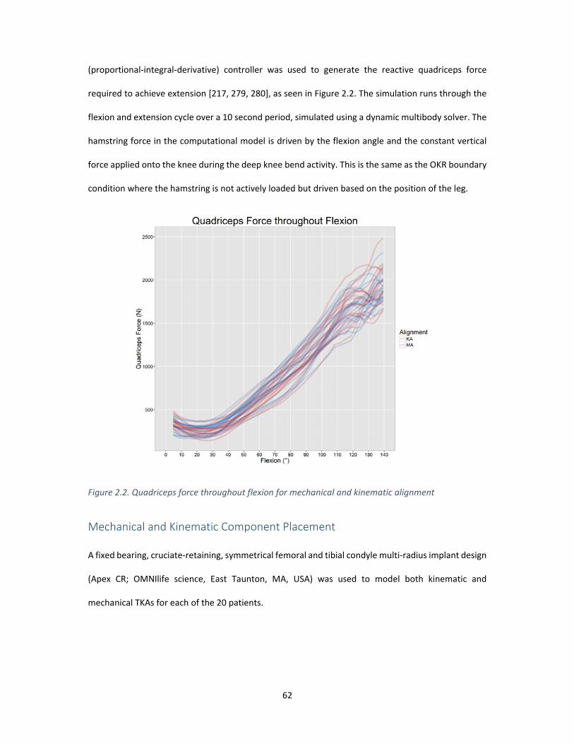
62

(proportional‐integral‐derivative) controller was used to generate the reactive quadriceps force

required to achieve extension [217, 279, 280], as seen in Figure 2.2. The simulation runs through the

flexion and extension cycle over a 10 second period, simulated using a dynamic multibody solver. The

hamstring force in the computational model is driven by the flexion angle and the constant vertical

force applied onto the knee during the deep knee bend activity. This is the same as the OKR boundary

condition where the hamstring is not actively loaded but driven based on the position of the leg.

Figure 2.2. Quadriceps force throughout flexion for mechanical and kinematic alignment

Mechanical and Kinematic Component Placement

A fixed bearing, cruciate‐retaining, symmetrical femoral and tibial condyle multi‐radius implant design

(Apex CR; OMNIlife science, East Taunton, MA, USA) was used to model both kinematic and

mechanical TKAs for each of the 20 patients.

63

Figure 2.3. Simulation showing boundary conditions and ligaments present in the computational model

(LCL, anterior MCL, posterior MCL, anterior PCL, posterior PCL). Ligaments were modelled as non‐linear

springs. Ligament forces were illustrated with the red lines.

The mechanically aligned femoral components were aligned in the coronal plane perpendicular to the

mechanical axis of the femur and rotated to be parallel with the projection of the surgical

transepicondylar axis. Translationally, the femoral components were placed such that the most distal

condyle of the native femur was level with the most distal point on the condyle of the implant, and

likewise for posterior placement [281].

Femoral component flexion and size were then set by incrementally flexing the component until the

anterior flange was flush to the anterior surface of the femur. A maximum of 5° flexion was used as

an upper limit before an upsized component was selected. Medial‐lateral positioning was performed

to result in equal amount of exposed bone on the medial and lateral sides.

The tibial component was placed perpendicular to the mechanical axis for all 20 mechanically aligned

simulations and rotated to match tibial AP rotational axis defined above. The component was placed

64

proximally to match the resection level of the thinnest tibia insert and had its medial‐lateral and

antero‐posterior position chosen to maximize coverage subject to those orientations. Posterior slope

for all tibial components was set at 3° from a line perpendicular to tibia mechanical axis.

Coronal view Sagittal view Axial view

Mechanical

(a)

(b)

(c)

Kinematic

(d)

(e)

(f)

Figure 2.4. Mechanically aligned femoral component (a), (b) and (c); kinematically aligned femoral

component (d), (e) and (f) in coronal, sagittal and axial views.

For the kinematically aligned knees, the femoral component was positioned such that the distal and

posterior condyles of the femoral component match the joint line of the native femur. The component

was then flexed and upsized as needed to avoid femoral component notching. For the tibial

component, rotation was defined by a best fit ellipse drawn on the lateral plateau of the tibia in order

to replicate the intra‐operative technique described by Howell et al [269]. Posterior slope of the tibial

component was set at 3° less than the posterior slope of the native medial condyle. Coronal plane

alignment was set level to tibia joint line and proximalised to match the resection level of the thinnest

65

tibia insert. Medial lateral and antero‐posterior placement of the component was performed to

optimize coverage. No medial tibial bone wear was encountered for patient’s included in this study.

For both the kinematic and mechanically aligned knees, patella implantation was modelled as an onlay

patella matching the resected surface at its posterior apex with an 8mm thickness patella button. The

largest patella button that could fit on the resected surface without overhang was implanted and

centred on the resected plane. The resection plane was drawn parallel to the patella tendon‐

quadriceps tendon attachment point axis and the femoral transepicondylar axis projected from the

CT scan. Components position of each subject was checked by experienced surgeons (JR, SH).

Coronal view Sagittal view Axial view

Mechanical

(a) (b)

(c)

Kinematic

(d)

(e) (f)

Figure 2.5. Mechanically aligned tibia component (a), (b) and (c); kinematically aligned tibia

component (d), (e) and (f) in coronal, sagittal and axial views. Tibia height was positioned to the tibia

center for visualisation purpose only. In computational model, the tibia height was positioned to fit

10mm poly thickness.

66

Figure 2.6. Ellipse used to define kinematic rotation angle and its angle relative to tibial AP rotational

axis

Data Analysis

Kinematics was assessed using an implant to implant reference frame for both mechanical and

kinematic alignment simulations and were based on the Grood‐Suntay measurement system [27].

Reporting kinematics to bone based reference frames was trialled however the native mechanical axes

results were dominated primarily by the static effects of component placement relative to the bone.

Static placement of the implants in kinematic alignment was done independently.

Component placement for the kinematically aligned knees relative to the mechanical axes was then

assessed. The simulated closed‐kinetic‐chain knee extension was performed, and measurements of

position were extracted. The medial and lateral flexion facet centre (FFC) condyles were identified as

the point equidistant from the most distal and posterior planes of the implant, as the multi radius

implant design did not have a single flexion centre. These points were used as the reference points for

measuring the movement of the femoral component relative to the tibia throughout the motion. The

medial and lateral FFC measurements were taken from these reference points to the lowest dwell

point on the tibial insert. Measurements were rescaled about the femoral AP measurement to

account for implant size geometry.

67

Rollback was measured from the centre of these two FFC points to the tibial dwell point posterior

translation of the transepicondylar line, hence is the average of the medial and lateral FFC translation

measurements. The internal‐external rotation measurement was the angle between the femoral and

tibial components projected onto the tibial component plane. Patella lateral shift was defined as the

translation from the centre of the patella button relative to the centre of the tibial insert, with positive

in the lateral direction and negative in the medial direction. Patella external tilt was defined as

external rotation of the patella relative to the transepicondylar axis of the femur projected onto the

tibial plane.

Results

Simulation Component Alignment for Kinematically Aligned Knees

Native coronal alignment (hip‐knee‐ankle angle) for all knees as measured from CT scan had a mean

of 3.1° ± 5.7° varus (range 8.7° valgus to 11.8° varus).

For mechanically aligned knees the femoral and tibial components were 0° to the mechanical axis. For

kinematically aligned knees the mean tibial component coronal and axial alignment was 3.0° ± 2.4°

(range ‐1.8° to 7.2°) varus to the mechanical axis and 7.2° ± 6.6° (range ‐9.4° to 15.4°) internal to tibial

AP rotational axis respectively for kinematically aligned knees. Both component alignment parameter

means were significantly different from mechanically aligned knees (0° varus and 0° rotation) (p <

0.05). Tibial slope in the kinematically aligned knees had a mean value of 4.6° ± 2.8° (range 0° to 11.2°).

Kinematically aligned tibial slope mean was also statistically different to the mechanically aligned tibia

slope (3° slope) (p < 0.05).

The mean femoral component coronal and axial alignment for kinematically aligned knees was 3.0° ±

2.3° (range ‐0.8° to 7.2°) valgus to the mechanical axis and 2.5° ± 1.6° (range ‐0.2° to 5.4°) internal to

the surgical transepicondylar axis respectively. As with the tibial component placement, both

component alignment parameter means were significantly different from mechanically aligned knees

68

(p < 0.05). Femoral flexion in the kinematically aligned knees had a mean value of 2.4° ± 1.7° (range 0°

to 5°, as per the planning process). Femoral flexion mean in the mechanically aligned dataset had a

mean value of 3.3 ± 1.7° (range 0° to 5°) and was not statistically different to that of the kinematically

aligned cases.

Figure 2.7 shows tibial and femoral component alignments for kinematically aligned knees. The

horizontal and vertical lines represent 0° coronal and 0° axial alignment respectively. The cross section

between the two lines is the mechanical alignment.

Figure 2.7. Coronal and axial component alignment for kinematically aligned knees. Left figure shows

the tibia component alignment. Right figure shows the femur component alignment. The cross section

of the 0° horizontal and vertical axis represents mechanical alignment.

Figure 2.8 shows kinematic femoral and tibial component coronal alignment shaded by the native

coronal alignment angle. The reference lines represent a 3° varus (blue), neutral (black) and 3° valgus

(red) as the final coronal alignment. There was variation in the level of joint line obliquity with a given

tibio‐femoral coronal alignment. However, a trend between the native and kinematic tibio‐femoral

69

final alignment is present. Linear regression of final alignment as a function of native alignment yields

an R2 of 0.75.

Figure 2.8. Kinematic alignment for femoral and tibial component valgus and varus angle shaded by

the native coronal varus angle. The reference lines represent a 3° varus (blue), neutral (black) and 3°

valgus (red) as the final coronal alignment. Mechanical alignment for femoral and tibial component is

at zero (black square).

Simulated Tibio‐Femoral Kinematics

Tibio‐femoral kinematic results are shown in Figure 2.9. Statistically significant differences for paired

t‐tests at every time parameter were found (p < 0.05), with the exception of femoral AP translation

70

from 30° of flexion and lower. The difference between the mean results for medial FFC AP translation

for the kinematic and mechanical simulations starts at 0.4 ± 0.9mm at 5° flexion, increasing steadily

to 1.7 ± 1.4mm in deep flexion, kinematically aligned being anterior to mechanical. The lateral femoral

FFC mean AP translation difference is 0.4 ± 0.6mm at 5°, increasing to 2.9 ± 1.9mm in deep flexion

with mechanically aligned anterior. The change in medial and lateral femoral FFC throughout flexion

also implicitly describes the tibio‐femoral internal‐external rotation; Kinematically aligned knees’

lateral femoral FFC translates more posteriorly and medial femoral FFC translates more anteriorly than

that of mechanically aligned knees’, as flexion increases. Thus there is more external rotation of

kinematically aligned knees. Also, there is relatively little difference in rollback behaviour, starting

with no difference peaking at 0.8 ± 0.9mm at 96°, kinematically aligned posterior to mechanical.

71

Figure 2.9. Tibio‐femoral kinematic results for knee flexion. Red lines are kinematic alignment and blue

lines are mechanical alignment. Solid lines are averages of each alignment. (a) and (b) medial and

lateral flexion facet centre (FFC) antero‐posterior drift from the lowest point of the tibial insert. Positive

values indicate anterior translation. (c) Femoral‐Tibial internal external rotation. Positive values

indicate external rotation. (d) Femoral AP translation relative to the lowest point of the tibia insert.

Simulated Patello‐Femoral Kinematics

The patello‐femoral kinematic results are shown in Figure 2.10. Patella lateral shift exhibited

statistically different parameter values for measurements of flexion between 10 and 40° and at angles

(a) (b)

(d) (c)

72

greater than 80°. Patella lateral shift for both alignment paradigms displayed a tendency towards

medialising throughout the flexion cycle, though trend lines are different.

After starting in a common position, the kinematically aligned patellae tended towards shifting

medially, peaking at 15° flexion where they were placed 1.8 ± 1.2mm more medial. The kinematically

aligned patellae then tracked without further medial lateral shift while the mechanically aligned

continue to drift medially, finishing in deep flexion 2.2 ± 1.6mm medial. Mean differences in patella

lateral tilt under kinematic and mechanical alignment are significant up to 30° of flexion (p=0.05).

Kinematic alignment begins the simulation at 2.7° ± 2.1° more internal tilt relative to the mechanically

aligned at 5° flexion, with the kinematically aligned knees tilting internally by a mean 3.5° while the

mechanically aligned knees are 0.8°. The means converge until about 60°, where they effectively show

identical movement into 5° external tilt at 140° flexion.

Intra‐patient differences for patella tracking are high, however, with the difference in tilt for a given

patient with either alignment approach ranging from 6° more externally titled to 6.5° more internally

tilted.

Figure 2.10. Patello‐femoral kinematic results for patella external tilt (left) and patella lateral shift

(right) for knee flexion. Red fine lines are kinematic alignment and blue fine lines are mechanical

alignment. Solid lines are averages of each alignment.

73

Discussion

Recent data has challenged the importance of traditional mechanical alignment philosophy [267].

Recently, Bellemans et al [10] have introduced the concept of “constitutional varus”, which

hypothesizes that correction to a neutral mechanical alignment may not be “normal” for a significant

proportion of the population. Their study showed 32% of asymptomatic men and 17% of

asymptomatic women possess a natural mechanical alignment of 3° varus or more.

In conjunction with this principle, several surgeons have supported the restoration of kinematic,

rather than mechanical, alignment in TKA [202, 205, 269] and Ji et al [282] reported that native and

‘healthy’ joint line were one and the same for Kinematically aligned knees. However, kinematically

aligned knees shows lack of consistency regarding patient outcomes, survivorship, and surgical

technique [170, 196, 202, 205, 269, 270]. Therefore, it remains unclear what are the optimal

alignment targets for TKA despite of the emphasis on alignment philosophies for TKA.

Recently, Ishikawa et al [261] used computational model to analyse the kinematics of kinematically

aligned knees. Their study suggests kinematically aligned knees produces near‐normal knee

kinematics. However, only a single model was used in the analysis and therefore the kinematics

outcomes reported were limited.

In this study, pre‐operative non‐weight bearing CT scans of diseased joints in 20 patients were used

to compare kinematic and mechanical alignment in a validated computational simulation. From

patient CT scans, native coronal alignment was determined, and kinematic and mechanical alignment

were planned (Figure 2.8). Ishikawa et al [261] used a clinically derived average kinematic alignment

at 3° tibial component varus and 3° femoral component valgus which is equivalent to coordinates (3,3)

on Figure 2.8. Our average alignment values were similar to reported alignment in clinical kinematic

alignment studies [261, 282]. However instead of using an average kinematic alignment, our study

accounts for significant variation of patient pre‐operative anatomy.

74

Results for kinematic alignment (Figure 2.8) showed there was variation in the level of joint line

obliquity with a set tibio‐femoral coronal alignment. However, a trend between the native and

kinematic tibio‐femoral final alignment was observed. Any variation observed most likely occurred

due to a condition of the pre‐operative diseased joint and the wide range of adjustments necessary

to attain kinematic alignment. When kinematically aligned, femoral components on average resulted

in more valgus alignment to the mechanical axis and internally rotated to surgical transepicondylar

axis whereas tibia component on average resulted in more varus alignment to the mechanical axis and

internally rotated to the tibial AP rotational axis. This is consistent with other reports [205, 269].

In regards to tibio‐femoral kinematics, both kinematic and mechanical alignment resulted in a broad

trend towards anterior translation of the femoral component up to 30° flexion, followed by posterior

translation as flexion increases (Figure 2.9). The kinematically aligned knees experience external

rotation of the femoral component on the tibial component during flexion, with the angle increasing

steadily from 1.2° ± 1.5° at 5° flexion to 5.9°± 3.3° at 140° flexion. This internal rotation of the femur

relative to the tibia as the knee reaches full extension is comparable to screw home mechanism

observed in native knee motion [15]. This effect is less so for mechanically aligned knees.

In regard to patello‐femoral kinematics, for both kinematic and mechanical alignment there was high

intra‐patient differences for patella tracking (Figure 2.10). However, the difference in tilt for a given

patient with either mechanical or kinematic alignment ranged from 6 degrees more externally titled

to 6.5 degrees more internally tilted. There was less medial movement of the patella in deep flexion

in kinematic aligned than mechanically aligned knees, though it arrived as its medial‐lateral position

earlier in the flexion. Differences in component alignment and potential impact on Q angle could

explain some of the variation seen in patella‐femoral kinematics for kinematically aligned knees.

Results for tibio‐femoral kinematics for flexion and rotation as well as patello‐femoral kinematics for

tilt and shift were similar to that of previous computational biomechanical studies [217, 245, 261, 274,

275]. Variations existed primarily due to patient CT input, on which knee joint testing rig was

75

simulated, e.g. Oxford Knee Rig or Kansas Knee Simulator, or if the implant was cruciate retaining (CR)

or substituting (PS), or the alignment strategy simulated.

Our results for tibio‐femoral kinematics for flexion and rotation using both mechanical and kinematic

alignment closely match results reported by Ishikawa et al [261]. All models exhibited anterior

translation of the femoral component relative to the tibia during the early flexion phase and then

posterior translation as flexion increased. The anterior translation from 0° to 30° of flexion was similar

bilaterally in all models.

Patella lateral shift kinematics also replicated a similar pattern of mechanical alignment to that

reported by Ishikawa et al [261]. However, patella lateral shift kinematics for kinematic alignment as

well as patellar external tilt for both alignments varied markedly between our results and those

reported by Ishikawa [261]. In the study reported by Ishikawa et al [261], in the kinematic alignment

models the patella tilted more externally relative to the femoral component at 0° and 30° and after

60° increased in all models. It was similar in our study until 60‐70° and then tilting plateaued.

Plateauing after 60° flexion was also reported by Kobayashi et al [283] using healthy subjects in an in

vivo study. Other explanations for this difference could be patient anatomy; Ishikawa study analysed

1 subject versus this study analysed 20 subjects, model assumptions, patellar button size or design of

the intercondylar notch and anterior patella groove of the femoral component.

There were several limitations in this study. The study involved 20 subjects only and this may be

insufficient given how variable knee alignment is across the population. Firstly, this study only

assessed one implant design. The implants used in this study were multi‐radius femoral component

with a single design fixed bearing cruciate retaining TKA. Therefore, the results may not be applicable

to other knee designs nor to mobile bearing or posterior stabilised knees. Also, the kinematics

analysed were for closed‐kinetic‐chain knee extension and therefore functions such as walking or stair

climbing may not be comparative. Furthermore, only kinematics was compared in this study. Ligament

76

forces and internal joint forces were not compared in this study as the computational model only

validated for kinematic outputs.

The simulation model was subject to assumptions and variables common to many computational

models: boundary conditions and muscle forces were assumed, only the lower extremity was

modelled, there was limited soft tissue representation and cartilage was not accounted for. Such

assumptions and variability are consistent with other computational modelling as well as in vitro

modelling studies. However, computational modelling does offer the ability to simulate kinematics of

different alignments on the same subject and thereby be potentially used as a predictive tool for pre‐

operative scenarios. Moreover, there are a number of studies that have shown that computational

models could predict forces and kinematics that compared favourably to those found experimentally

or in vivo fluoroscopy [217, 245, 274, 275].

Conclusions

In conclusion, kinematic alignment had more variation than mechanical alignment for all tibio‐femoral

and patella‐femoral kinematics. This was particularly true for tilt and shift of the patella‐femoral joint

for kinematically aligned knees. Kinematic alignment corrects long leg alignment to a patient specific

alignment which depends on the preoperative state of the knee. Also, when kinematically aligned,

femoral components on average resulted in more valgus alignment to the mechanical axis and

internally rotated to surgical transepicondylar axis whereas tibia component on average resulted in

more varus alignment to the mechanical axis and internally rotated to the tibial AP rotational axis.

The use of computational models has the potential to predict which alignment, kinematic or

mechanical, could improve knee function patient specifically.

77

Chapter 3

Accurate Determination of Post‐operative 3D Component Positioning in Total Knee Arthroplasty: The AURORA Protocol

This chapter was published in Journal of Orthopaedic Surgery and Research

Wakelin EA, Tran L, Twiggs JG, Theodore W, Roe JP, Solomon MI, Fritsch BA, Miles BP., "Accurate determination

of post‐operative 3D component positioning in total knee arthroplasty: the AURORA protocol," (in eng), J Orthop

Surg Res, vol. 13, no. 1, p. 275, Oct 30 2018.

In Chapter 2, we developed a knee computational model that replicates Oxford Knee Rig (OKR) deep

knee bend and was able to demonstrate the model capability in demonstrating kinematic differences

with different implant positions on the same subject. It was later realized that there was inconsistency

in registration technique used to transform computational model and experimental reference frame

in the first computational model validation. The computational models used for the first validation

78

were derived from post‐op CT with implant CAD model registered against the scan. The anatomical

landmarks were also derived from post‐op CT which its determination affected by the metal flare in

the post‐op CT. Additionally, the experimental data was not registered accurately to the

computational model reference frame resulting in inconsistent landmark definition used to compare

the experimental kinematics and simulated kinematics.

This chapter describes a new technique to measure post‐operative component position from

Computed Tomography (CT). The technique developed involves registering both implant and

preoperative bone 3D CT segmented models to a postoperative CT reference frame. Doing so allowed

for a more accurate definition of component placement in all 3 planes, going beyond what 2D

radiography can provide. The technique developed also eliminates the necessity to determine

anatomical landmark from post‐op CT, preventing inaccuracy of landmark determination due to metal

flare.

This chapter was written as an independent published article, as such the content was targeted for

more general readers. While not the primary author of this paper, my contribution to the publication

includes the conception of the registration technique, development of the step‐by‐step instructions,

designed and supervised the reproducibility study. In addition, I assisted in writing and reviewing the

manuscript. I contributed 70% to the research design, 50% on data collection and 50% of manuscript

preparation and review. Permission from the primary author has been provided.

79

Introduction

Dissatisfaction amongst total knee arthroplasty (TKA) is the result of a complex relationship between

the patient anatomy, prosthesis design and position, and other patient specific factors. Prosthesis

malalignment has been linked to poor patient outcomes in which coronal and axial malalignment have

been most closely studied [204, 284]. To have confidence in the correlation between component

alignment and outcome, the method used to determine component placement must be accurate and

reliable.

Component alignment refers to the angular difference between the prosthetic components and

patient derived antero‐posterior (AP), medio‐lateral (ML) and superior‐inferior (SI) anatomic axes. This

measurement has traditionally been the focus of post‐operative analysis in TKA due to the ease of

measurement [285‐287]. Component placement refers to the translational movement of the

prosthetic components along these patient specific axes. Due to difficulty in identifying the origin of

these axes and accurately determining translation in space, component placement has been less well

investigated. To understand the holistic effect of the TKA components on knee kinematics, both the

alignment and placement must be taken in to account. Here we term the combination of component

alignment and placement as ‘component position’.

The pre‐operative state of the patient is a critical source of missing data from most analyses which

prevents accurate reporting of component position. Bony resections cannot be accurately determined

from a post‐op analysis alone and as a result there is very little data available on the outcome of TKA

as a result of the modification of the anatomy [288, 289], highlighting the need for improved post‐

operative analysis techniques. Nevertheless, studies have investigated range of movement and

maximum flexion as a function of the posterior condylar offset (PCO) [290‐292]. In these publications

a greater PCO resulted in higher maximum flexion due to reduced steric hinderance. Pre‐ and post‐

80

operative measurements however were limited by the use of ML x‐rays, indicating that the

relationship must be strong to overcome such errors.

Alteration of the joint line and flexion/extension gaps are associated with a change in joint kinematics

[293] and patient outcome [294]. In these studies, patients with less change to the coronal joint line

reported improved WOMAC and Knee Society Clinical Rating Scores. Identification of such changes

however can be difficult, as the joint line and joint gaps can be modified without affecting the

appearance of the component alignment [287]. To better understand the effect of bone resections,

joint line and gap modification, accurate pre‐operative geometry data is required. Similarly, Bengs et

al.[295] found that increasing patella button thickness without increasing the patella resection,

decreased maximum passive flexion. Identification of appropriate patella resection for a given button

thickness would not be possible with traditional post‐operative analysis techniques.

Traditional methods of assessing TKA component alignment, including short leg x‐rays [296‐298], long

leg x‐rays [299], and post‐operative 3D imaging only [300‐304], have been shown to suffer

inaccuracies from anatomic variability, projection errors, and difficulty in identifying patient specific

landmarks from the post‐operative imaging. To improve landmarking and component placement

accuracy, a pre‐operative CT is required. Fortunately, CT imaging is rapidly becoming a standard of

care in pre‐operative planning for TKA [305], and is available for a wide range of patients. Pre‐

operative CT imaging allows a volumetric registration of the pre‐operative and post‐operative bones

and component geometries in 3D space eliminating any anatomic assumptions and projection errors.

The models can then be used to determine bony resections and component placement. A method to

compare the pre‐operative state of the knee to the post‐operative component position and bone

resections, in which accuracy has not been affected by component flare has not yet been achieved.

Here we introduce a method of 3D reconstruction which utilises both a pre‐operative and post‐

operative CT scan to determine the post‐operative component position in TKA. The method may be

extended to any joint replacement and is termed here the Australian Universal Resection, Orientation

81

and Rotation Analysis (AURORA) protocol. Landmarks and bone models unaffected by component

flare obtained from the pre‐operative scan are transformed into the post‐operative frame of

reference. Component position as defined by the landmarked patient specific axes and bony

resections are reported. The reproducibility and reliability of this method are presented and compared

to other post‐operative analysis techniques. This registration method is considered accurate and

suitable to be used when absolute difference in registration results is less than 1° and 1mm and

repeatability intraclass correlation coefficient of at least 0.9.

Methods

CT Protocol

A series of patients received long leg pre‐operative CT scans for routine pre‐operative planning of TKA

surgery [306] and to design patient specific instrumentation. Ethics approval for all data collection and

accessing information from a joint registry for this study was approved by Bellberry Ethics (Sydney,

Australia) (approval 2012‐03‐710). The same protocol is followed for post‐operative CT imaging. This

protocol requires the patient to be in supine at the isocentre of the gantry, with both legs fully

extended and parallel to the horizontal plane. The legs are straightened and maintained in a relaxed

position. Image acquisition involves a full leg pass CT scan taken through both limbs with all images

taken in the same field of view, see Figure 3.1. This allows detection of any patient movement during

the scanning process. Transverse slice thicknesses of 1.25 mm are taken, with less than 1 mm slices

taken within the sagittal and coronal axis.

All patients investigated here had a TKA using OMNI APEX implants (Raynham, MA), from 4 different

surgeons using 4 different techniques. Patients were randomly selected from a database of over 2000

TKA surgeries.

The CT dose is calculated by multiplying the dose‐length‐product (mGy.cm) provided as supporting

information with the CT scan, by the length of the CT scan in which the patient is imaged. The dose

82

value is then converted to an effective dose based on anatomic conversion coefficients presented by

Saltybaeva et al. [307] to allow comparison between different CT protocols. Movement in the scan

can affect both individual bone and long leg measurements. Movement is detected by an engineer

assessing the scan before processing. All patients were randomly selected from a database of patients

scanned over a 3‐month period previously confirmed to have not moved.

83

Figure 3.1. Single‐pass CT scan through both limbs

Image processing and Volumetric Registration

3D reconstructed patient femur and tibia bones are generated within the pre‐operative planning

process through semi‐automated segmentation, used to landmark and identify points of interest by

biomedical engineers using the 3D imaging software, ScanIP (Simpleware, Exeter UK). The accuracy of

84

the landmarking process depends on the CT slice thickness. In this study, 1.25mm axial slice increment

was used in CT protocol and therefore the landmarking accuracy is 1.25mm. The patient bones are

converted to stereolithography (STL) files and manually landmarked twice by different engineers. The

landmarking was done on the generated STLs with combination of reviewing them in the 2D CT slices.

If any landmarks taken by first and second engineer differ by a threshold value (in this case 4 mm), the

landmark was reviewed by a third trained engineer. Landmark references were used to define patient

specific bone axes and soft tissue attachment sites, see Figure 3.2A. The femoral and hip centres are

landmarked to define the mechanical axis of the femur. The tibial mechanical axis is defined from the

midpoint of the lateral and medial malleoli to the midpoint of the medial 1/3 of the tubercle and PCL

insertion. The tibial AP axis is defined along the medial 1/3 of the tubercle and PCL insertion, while the

Transepicondylar Axis (TEA) is defined along the medial sulcus to the lateral epicondyle on the femur.

These axes are used to define a frame of reference from which implant position may be calculated.

Using the post‐operative full leg CT scan, 3D post‐operative femur and tibia bone sections unaffected

by the component flare are segmented, see Figure 3.2B. 3D registration is then performed, by

registering the pre‐operative femur and tibia models into the post‐operative CT with reference to both

the imaging and newly generated post‐operative bone models, see Figure 3.2C. Point‐to‐point

registration is performed on CAD models of the implanted prosthesis and segmented prosthesis

models from the CT, see Figure 3.2C. All registration is refined using model outlines viewed in the full

leg CT scan. A second engineer reviews both the registered femur and tibia bones, and the femoral

and tibial implant components to further refine both bone and implant positions within the CT scan.

Euler transform matrices are obtained from the resulting registered pre‐operative bones and used to

transform the pre‐operative bone landmarks into the post‐operative CT reference frame. Using the

transformed landmark references, component alignment and placement are determined within the

local reference frames from the defined axes of landmarks identified pre‐operatively.

85

Figure 3.2. Post‐operative process workflow showing a) pre‐operative bone segmentation and

landmarking, b) segmentation of post‐operative bones and components, and c) registration of pre‐

operative to post‐operative bones and components.

Accuracy testing

ScanIP software an FDA approved medical software specifically designed to process medical imaging

and registration of 3D models. Therefore, the software measurements would have been validated

before FDA approval. Further validation study was conducted internally to validate ScanIP

measurement outputs (refer to Appendix C). Since ScanIP software outputs had been validated, the

accuracy of the described registration method is dependent only on the operator who perform the

tasks. Therefore, the accuracy is described using reproducibility and reliability analysis.

Reproducibility

Two primary TKR patients were processed post‐operatively twice by 3 engineers in a 2‐week period.

Patient CT scans were segmented and registered by an engineer and then reviewed by a second. The

same case was processed again by the initial engineer on another day at a different time of day and

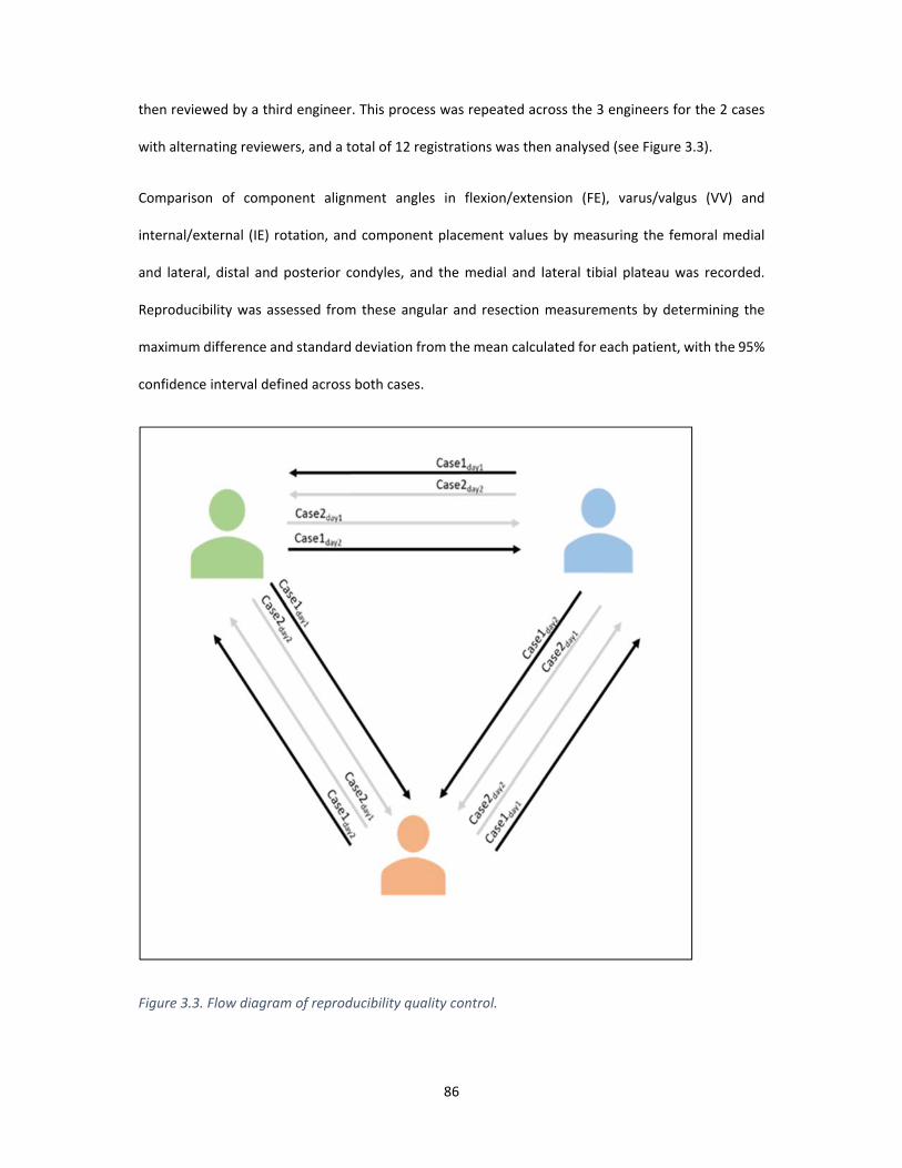
86

then reviewed by a third engineer. This process was repeated across the 3 engineers for the 2 cases

with alternating reviewers, and a total of 12 registrations was then analysed (see Figure 3.3).

Comparison of component alignment angles in flexion/extension (FE), varus/valgus (VV) and

internal/external (IE) rotation, and component placement values by measuring the femoral medial

and lateral, distal and posterior condyles, and the medial and lateral tibial plateau was recorded.

Reproducibility was assessed from these angular and resection measurements by determining the

maximum difference and standard deviation from the mean calculated for each patient, with the 95%

confidence interval defined across both cases.

Figure 3.3. Flow diagram of reproducibility quality control.

87

Reliability

To describe the interobserver reliability, 11 TKR patients were processed post‐operatively between 2

engineers. Each case was reviewed by a third and fourth engineer, with refinement of the bone and

component registration made by the reviewing engineer if necessary. A set of 22 results were

produced for comparison of the 3 rotation axes across two components and 6 resection

measurements. The intraclass correlation coefficient (ICC) was calculated for each of the

measurements. An ICC value of 1 shows perfect reliability, values greater than 0.9 indicates an

excellent result, 0.81 to 0.9 is very good, 0.76 to 0.80 is good, 0.5 to 0.75 is moderate and <0.50 is

considered to show poor reliability [308, 309].

Results

Radiation Dose

The average effective radiation dose received per CT scan using this protocol is 1.24 ± 0.96 mSv. This

dose is compared to other CT and radiography protocols in Figure 3.4. The average received dose is

lower than all protocols shown in the figure with the exception of the most recent Imperial Protocol

[288] and a standard AP radiograph. The spread of values shown for the AURORA CT protocol used

here reflect the large range of patient sizes scanned. Smaller patients receive a correspondingly lower

dose of radiation and vice versa for larger patients.

88

Figure 3.4. Comparison of the AURORA CT protocol with a barium enema and other relevant protocols

for determining prosthesis positioning. AURORA protocol dose is calculated from CT reports, all other

data taken from Henckel, et al [288].

Using the AURORA protocol, patient movement in the CT scan may be detected at any point along the

length of the bone. In previous methods, such as the Perth CT and Imperial protocols, movement in

the mid femur and mid tibia will not be detected, leaving any measurements to propagate through

the protocol as an error. In a database of CT scans obtained for routine pre‐operative planning of TKA,

the rate of scans identified with movement over a 3‐month period is 6.78% (total number of scans:

118). Of this fraction, all movement in the scans were detected in the mid femur and mid tibia regions.

Reproducibility

The alignment reproducibility results generated from three engineers processing two cases at two

different time points which were then QC checked are shown in Table 3.1. The maximum difference

from the mean angle is shown for each case. In both cases the maximum difference is reported for

tibial component axial rotation, of 0.9⁰ for case 1 and 0.7⁰ for case 2. In all other angles, the maximum

89

difference in rotation is ≤ 0.5⁰. The confidence intervals in all cases are less than 0.3⁰ with the

exception of tibial tray IE rotation, which is 0.6⁰ for case 1, and 0.4⁰ for case 2.

The bony resection thicknesses are a proxy measure for the accuracy of measuring component

placement and are shown in Table 3.2 for the distal medial and lateral condyles, posterior medial and

lateral condyles, and tibial medial and lateral plateaus. The maximum difference from the mean

resection is shown for each case. In both cases the maximum difference is reported for the medial

tibial plateau, of 0.5 mm for case 1 and 0.3 mm for case 2. In all other resections, the maximum

difference in resection is ≤ 0.3 mm. The confidence intervals in all cases are less than 0.3 mm.

90

Table 3.1 Reproducibility results showing the difference in calculated component angular alignment

across two cases performed by three engineers at two different time points. The maximum average

difference for each case and a 95% confidence interval is shown for all three axes of rotation for the

femoral and tibial components.

Case Operator Run Femoral Component Alignment Tibial Component Alignment

F/E V/V IE F/E V/V IE

Case 1 Sim Eng A Run 1 1.1 ‐0.6 ‐0.8 7.1 0.6 5.9

Case 1 Sim Eng A Run 2 1.0 ‐0.5 ‐1.2 7.0 0.4 6.2

Case 1 Sim Eng B Run 1 1.0 ‐0.8 ‐1.5 7.0 0.5 4.5

Case 1 Sim Eng B Run 2 0.8 ‐0.7 ‐0.8 7.4 0.4 4.7

Case 1 Sim Eng C Run 1 1.1 ‐0.6 ‐1.8 6.9 0.8 5.5

Case 1 Sim Eng C Run 2 1.1 ‐0.4 ‐1.0 7.2 0.6 5.9

Maximum Difference from

Average (⁰) ± 95% CI 0.2 ± 0.1 0.2 ± 0.1 0.5 ± 0.3 0.3 ± 0.1 0.2 ± 0.1 0.9 ± 0.6

Case 2 Sim Eng A Run 1 1.9 ‐0.9 0.1 8.2 1.5 3.0

Case 2 Sim Eng A Run 2 2.3 ‐0.8 ‐0.1 7.7 1.8 2.7

Case 2 Sim Eng B Run 1 2.3 ‐0.7 ‐0.2 7.9 1.7 1.7

Case 2 Sim Eng B Run 2 2.1 ‐0.8 0.4 8.4 1.4 2.8

Case 2 Sim Eng C Run 1 2.0 ‐0.7 ‐0.2 7.9 1.0 2.3

Case 2 Sim Eng C Run 2 1.8 ‐0.8 0.0 8.4 1.5 2.8


Average (⁰) ± 95% CI 0.3 ± 0.2 0.1 ± 0.1 0.3 ± 0.2 0.3 ± 0.2 0.4 ± 0.2 0.7 ± 0.4

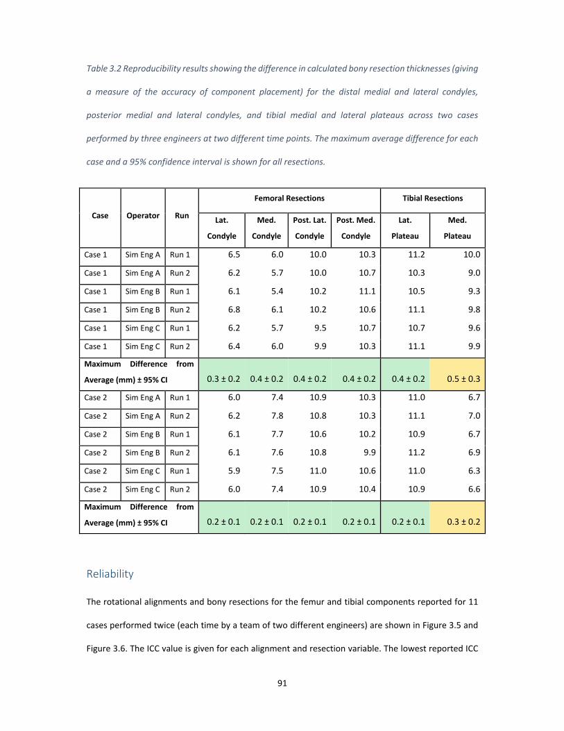
91

Table 3.2 Reproducibility results showing the difference in calculated bony resection thicknesses (giving

a measure of the accuracy of component placement) for the distal medial and lateral condyles,

posterior medial and lateral condyles, and tibial medial and lateral plateaus across two cases

performed by three engineers at two different time points. The maximum average difference for each

case and a 95% confidence interval is shown for all resections.

Case Operator Run

Femoral Resections Tibial Resections

Lat.

Condyle

Med.

Condyle

Post. Lat.

Condyle

Post. Med.

Condyle

Lat.

Plateau

Med.

Plateau

Case 1 Sim Eng A Run 1 6.5 6.0 10.0 10.3 11.2 10.0

Case 1 Sim Eng A Run 2 6.2 5.7 10.0 10.7 10.3 9.0

Case 1 Sim Eng B Run 1 6.1 5.4 10.2 11.1 10.5 9.3

Case 1 Sim Eng B Run 2 6.8 6.1 10.2 10.6 11.1 9.8

Case 1 Sim Eng C Run 1 6.2 5.7 9.5 10.7 10.7 9.6

Case 1 Sim Eng C Run 2 6.4 6.0 9.9 10.3 11.1 9.9


Average (mm) ± 95% CI 0.3 ± 0.2 0.4 ± 0.2 0.4 ± 0.2 0.4 ± 0.2 0.4 ± 0.2 0.5 ± 0.3

Case 2 Sim Eng A Run 1 6.0 7.4 10.9 10.3 11.0 6.7

Case 2 Sim Eng A Run 2 6.2 7.8 10.8 10.3 11.1 7.0

Case 2 Sim Eng B Run 1 6.1 7.7 10.6 10.2 10.9 6.7

Case 2 Sim Eng B Run 2 6.1 7.6 10.8 9.9 11.2 6.9

Case 2 Sim Eng C Run 1 5.9 7.5 11.0 10.6 11.0 6.3

Case 2 Sim Eng C Run 2 6.0 7.4 10.9 10.4 10.9 6.6


Average (mm) ± 95% CI 0.2 ± 0.1 0.2 ± 0.1 0.2 ± 0.1 0.2 ± 0.1 0.2 ± 0.1 0.3 ± 0.2

Reliability

The rotational alignments and bony resections for the femur and tibial components reported for 11

cases performed twice (each time by a team of two different engineers) are shown in Figure 3.5 and

Figure 3.6. The ICC value is given for each alignment and resection variable. The lowest reported ICC

92

variable is for femoral axial rotation, with an ICC of 0.93. These values are all above 0.9, indicating that

across all rotations and resections in both the femur and tibia, the protocol reports excellent reliability.

Figure 3.5. Reliability testing for femur and tibia placement showing the coronal, axial and sagittal

rotation reported by the method across 11 cases performed by two engineers, followed by two

additional engineers reviewing the placement. The ICC for each rotation in each component is reported.

All values are greater than 0.9 indicating excellent reliability.

93

Discussion

The maximum component alignment differences from the mean within this study are low compared

to previous literature and provide a confidence interval up to 10 fold narrower when compared to

protocols in which individual CT slices were investigated [300, 301, 304, 310], or only post‐operative

CT scans were available [311, 312]. The maximum error of < 1⁰ is similar to protocols using more

advanced techniques, such a computational edge detection, however these studies did not include

ICC coefficients, so an assessment of the repeatability was not possible [313]. The highest deviation

from the mean was the tibial IE rotation at 0.9⁰ and 0.7⁰ for the two cases, with a confidence interval

of 0.6⁰ and 0.4⁰ respectively. These values represent an 8 fold improvement in accuracy compared to

previous attempts to measure tibial rotation [314]. Previous attempts have reported difficulty in

measuring tibial IE rotation due to the variability in the landmarks required to define a useful axis

[315]. By combining the pre‐op and post‐op CT, the landmarks that define the AP axis can be identified

more easily than using post‐op CTs alone. Although there may still be some debate over which

landmarks are the most appropriate, this method allows points to be defined that accurately

reproduce an anatomic axis across multiple subjects. The origin of all axes may be redefined based on

future literature if needed.

The resulting resection level measures of the femur and tibia also show high reproducibility, with the

highest deviation seen for the medial tibial plateau resection at 0.5 mm and 0.3 mm between the two

cases and confidence intervals of 0.6⁰ and 0.4⁰, respectively. The magnitude of the error here,

however, is only slightly above the other resections, indicating that there may not be a systematic

reason for reduced accuracy when placing this component. Previous attempts have been made to

investigate the effect on TKA outcome arising from resection levels. These studies have mainly

focussed on the femur, particularly the posterior condylar offset [290, 316, 317]. These techniques

however have primarily relied upon fluoroscopic images, and planar x‐rays which were discussed

previously to be inaccurate, limiting the reliability of such studies.

94

Figure 3.6. Reliability testing for femur and tibia bony resections reported by the method across 11

cases performed by two engineers, followed by two additional engineers reviewing the placement. The

ICC for each rotation in each component is reported. are greater than 0.9 indicating excellent reliability.

Across both femoral and tibial component alignments and bony resections, this 3D pre‐operative

registration process shows excelled reliability, in which all ICC values report greater than 0.93. The

lowest reported ICC value of 0.93, resulting from the femoral axial IE rotation measure, is primarily

due to the difficulty of post‐operative registration of the femur component. The posterior condyles,

which dominate the axial rotation positioning, of the APEX implant used in this study are thicker than

the distal condyles (11 mm vs 9 mm) and tibial tray (~3 mm). As such, the CT flare is greater in these

regions, reducing the accuracy of the registration. The ICC values reported here are consistently similar

95

to or higher than other post‐operative analysis techniques [289, 304, 318] indicating this method is

not only accurate, but suitable for routine post‐processing by multiple users.

The high reproducibility and reliability of calculating both component alignment and bony resections

performed by surgeons, can lead to a better understanding of the influences of component alignment

and component placement. Current literature has thoroughly reviewed the influence of component

malalignment and poor patient outcomes [185, 319, 320]. Missing from all of these analyses however,

is an understanding of the patient’s preoperative anatomy, leading Hadi et al. [185] to conclude that

there is a dubious link between component malalignment and patient outcomes. From this post‐

operative analysis, we can begin to determine how the bony resections and the combination of

component placement and alignment influence outcome on a patient specific level in greater detail.

For example, the use of reliable bone resection measures from pre‐operative bones may provide

insight into the change of a patient’s soft tissue profile post‐surgery. From the pre‐operative CT scans,

comparative ligament lengths and change in length resulting from component alignment and

placement can be investigated from landmarked attachment sites. CT scans in this analysis however,

are performed in a non‐functional supine position, such that the distance between ligament

attachment sites may not be representative of the functional length of the ligament. Functional

imaging may be introduced to this workflow in future to this issue without a change in post‐processing

techniques.

The proposed 3D registration process for post‐operative analysis involves additional pre‐operative CT

imaging compared to other processes [288, 300]. Though this increases x‐ray exposure to the patient,

pre‐operative planning, generally requiring a CT scan, is becoming the standard of care for TKA [305],

such that the pre‐operative scans are not for post‐operative analysis alone. The protocol used here is

a low dose CT, with radiation exposure less than the typical yearly background radiation and similar

to protocols currently in use [288]. All patient movement identified in pre‐operative scans occurred in

the mid femur and mid tibia regions, indicating that protocols which did not include the mid femur

96

and tibia sections would report inaccurate component placement. The resulting error in component

position if these scans were used is the subject of further study.

Manual translation and rotation of the pre‐operative bones and component geometries into the post‐

operative CT scan is reasonably labour intensive, requiring on average 60 minutes to complete, before

the registration is quality control checked by a second engineer with additional experience. Further

refinement of the proposed post‐operative analysis process could include the use of an automated

registration method. A preliminary automated registration process using the Iterative Closest Point

method (ICP) [312] was performed on these cases. The registration time was observed to reduce to

approximately 2 minutes, from which the results were then fine‐tuned by one engineer and quality

control checked by a second engineer, representing a 30‐fold decrease in time. Further development

of the ICP method to optimise parameters around fitting regions of interest, reliability, and time for

analysis may allow accurate post‐operative analysis to be part of routine care and is the subject of

future studies.

Joint infection and component loosening are a cause of dissatisfaction and revision surgery. Joint

infection can be identified by swelling of the joint and pathology reports, however these are not

always conclusive. Combining component position as determined using the AURORA protocol with

SPECT imaging could identify bone metabolism associated with infection or component movement

[321]. Although current methods integrating SPECT imaging with CT do not improve the accuracy of

determining component placement, such methods may be used to augment a pre‐operative and post‐

operative CT 3D reconstruction to add metabolic activity.

The proposed post‐operative 3D registration method described here has some limitations. The current

time taken for this analysis as mentioned is approximately 60 minutes, this represents a high

engineering burden, and must be reduced to improve use in routine analysis. Commercially, TKA

component geometry varies between medical device manufacturers, forming a significant part of their

IP portfolio, as such, the component geometries must be obtained from the implant companies, which

97

may be difficult – limiting the generalisability of this technique to engineering firms with a close

relationship with implant companies. The reproducibility analysis performed here utilises 2 cases

processed at multiple time points by multiple engineers of equal training. To better understand the

reproducibility, particularly when processing outlier or severely pathological anatomy, a greater

number of cases should be analysed. Furthermore, this method requires pre‐op and post‐op CT. Even

though low dose CT is used for this method, there is still additional radiation and cost associated.

Other methods to assess component position such as bi‐planar x‐rays followed by 2D to 3D

registration offer a number of advantages over a CT, such as providing long leg assessments in a

functional state [322]. Such techniques however, may require fluoroscopic agents [323], may only

capture the region around the knee, and are performed on apparatus less widely available than

traditional x‐ray or CT machines, limiting its use [313].

Conclusion

Component alignment has been of great interest in total knee arthroplasty, however the focus has

previously been on achieved component alignment and identification of malalignment without regard

for the component placement or pre‐operative anatomy. The method presented here uses a low dose

CT scan to analyse the position and rotation of all components in 3D space, with comparison to the

pre‐operative anatomy, allowing surgical changes to the joint to be determined. The method shows

excellent reliability and reproducibility by removing sources of error that are typically associated with

post‐operative total knee arthroplasty analysis. Routine use of this analysis in TKA as well as other

joint replacement procedures will allow surgeons and engineers to better understand the effect of

component alignment as well as placement on outcome.

98

Chapter 4

A Technique for Kinematic Validation of a Low‐cost Subject

Specific TKR Model Derived from CT Scan

This chapter was submitted to journal Recent Advances in Arthroplasty

Willy Theodore; Joseph Little; Edgar A Wakelin; Justin Roe; Darryl D’lima; Mark Taylor; Brad Miles

99

Introduction

Total Knee Arthroplasty (TKA) is a highly successful surgical intervention that relieves pain and

improves the quality of life for osteoarthritis sufferers. Despite low revision rates, as many as 20% of

recipients remain dissatisfied with long term pain after surgery [141, 324, 325]. Component alignment

[326‐328] as well as patient specific anatomical variation [306, 329, 330] has been shown to alter the

kinematics and performance of the knee. Knee kinematics post‐TKA therefore, are a product of

complex interactions between the component design, component alignment, and patient specific

anatomic characteristics [140, 331, 332]. Understanding these complex interactions pre‐ and intra‐

operatively can help surgeons better plan surgery to achieve optimal outcomes.

Techniques such as ex‐vivo force‐controlled mechanical simulators [333‐336], video fluoroscopy [337]

and gait labs [338] have been used to study knee kinematics under simulated and real dynamic

activities. This process however is expensive and inefficient to iterate experiments over a wide variety

of variables (i.e. alignment and position of each component, variable anatomy etc.). Furthermore, ex‐

vivo testing is limited to cadaver specimens and therefore has limited applicability to be used as a tool

to study complex interactions pre‐operatively. Computational modelling however, is a scalable

alternative [339] that allows the study of both patient and surgical factors and their interactions on

knee kinematics.

In Chapter 2, we developed a knee computational model that replicates Oxford Knee Rig (OKR) deep

knee bend and was able to demonstrate the model capability in demonstrating kinematic differences

with different implant positions on the same subject. It was later realized that there was inconsistency

in registration technique used to transform computational model and experimental reference frame

in the first computational model validation. In previous chapter, we demonstrated a registration

technique to obtain accurate 3D implant position using pre‐operative and post‐operative CT. The

technique developed will be utilized in this chapter. It was also realized in the first model validation

100

that inconsistent landmark definition was used to compare the experimental kinematics and

simulated kinematics.

Previous model development that replicates OKR deep knee bend validation studies have compared

simulated kinematics against kinematics recorded in an experiment knee simulator with definition

described in the Grood and Suntay coordinate system [244, 246, 261, 340]. However, the landmarks

used to create the experimental kinematics were not identical to the landmarks used to create the

simulated kinematics. For example, Colwell et al [246] digitized bony attachments during the

experiment to calculate the experimental coordinate system but the simulated kinematics coordinate

system was created using scaled bony attachment sites. This resulted in fundamental difference in

kinematics definition. Furthermore, a previous study by Victor et al [305] reported that there is high

variability in anatomical feature localisation or landmarking, particularly from post‐operative CT

where metal flares present. Therefore, if only post‐op CT is used to define the cadaver computational

model, there is a high chance the anatomical axes digitized may not represent the true axes.

More recent studies have reported improved kinematics comparison technique however it is still

unclear whether the landmarks used in creating both coordinate system were identical [250‐252].

Kansas research group in their computational model studies [217, 341] dissected the knee specimen

after experiment and register the experimental digitized landmark points to the CT model using rigid

body fixtures. This method has a risk of unwanted movement of the fixtures during experiment

particularly after cutting and dissecting the bones which may introduce different relative landmark

position at different stages of experiment. Kia et al [342] and Vanheule et al [343] used different

workflow in their technique. They attached rigid markers onto the specimen bone before radiographic

imaging, allowing the rigid markers identifiable during image segmentation. The rigid markers were

also digitized in experiment to allow registration between the two reference frames. Registration

between experiment and computational model was done on identified features of the rigid markers.

101

In this study, we present a series of registration technique that transform experimental outputs from

a mechanical simulator to computational model reference frame in which the only digitization points

are from the implanted components. This ensures identical landmark definitions are used when

comparing model‐predicted and experiment kinematics, eliminating a source of error identified in

previous validation procedures. Further objective of this work was to use the described method to

validate a CT‐based subject‐specific computational model that incorporates literature‐based soft

tissue properties. The model was developed to have sufficient complexity to achieve accuracy in

kinematics when compared against experimental data while limiting invasive data capture to improve

clinical utility.

Method

Cadaveric Testing

Ten fresh‐frozen human cadaver knees underwent pre‐operative CT scans. TKA was then performed

on each of the cadaver knees with fixed‐bearing, ultracongruent (with PCL sacrificed), TKA

components (GMK, Medacta, Switzerland), after which a post‐operative CT was obtained.

A surgical navigation system (Stryker Navigation 4.0 Research Version, Kalamazoo, Michigan, USA) was

used to record kinematics throughout a deep knee bend. The accuracy of the Stryker navigation

system is 1° and 2mm [344]. Navigation arrays were attached to the femur, tibia and patella. The

implant geometry surface (IGS) of each component were then digitized, allowing the position of the

implants and bone to be mapped relative to the navigation arrays respectively. Figure 4.1 shows the

overview of experiment steps in a flow chart.

102

Figure 4.1. Overview of experiment procedure.

Each cadaver was mounted in a dynamic, quadriceps‐driven, closed‐kinetic‐chain knee simulator

based on the OKR design, as previously described [276]. Steel rods were cemented into the femoral

and tibial medullary canals, fixing the bones to the testing apparatus. The femoral rod was attached

with a lateral offset of 5° from the hip joint to reproduce the average anatomic valgus in the femoral

shaft [276]. The ankle joint was fixed rigidly to prevent translation, but the rotational degrees of

freedom were left unconstrained. The hip joint was positioned directly vertical to the ankle joint and

allowed to translate vertically, as well as rotate in flexion‐extension and varus‐valgus. A vertical load

was applied through the hip joint to generate a peak knee‐flexion moment of approximately 40 Nm,

similar to that reported for stair climbing after TKA [246]. The attached navigation arrays were tracked

using the navigation unit during the second half of the deep knee bend cycle, i.e during extension.

103

Computational model

A knee computational model (KCM), with subject specific inputs derived from a CT scan only and

designed to replicate the experimental mechanical simulator, was developed in rigid body modelling

software, ADAMS (MSC, California, US), as described in [345]. Image processing and segmentation was

performed on both pre‐op and post‐op CT’s taken for each cadaver using ScanIP (Simpleware, Exeter,

UK). The native geometry of the femur, tibia and patella were generated and anatomic landmarks

were recorded from the pre‐op CT on all bones to define local and global axes, as well as soft tissue

attachments, similar to those defined by Theodore et al [345], in which anatomic morphology and CT

pixel intensity were used to inform landmark positions. The pre‐operative bones and implanted TKA

CAD geometries were then registered to the post‐operative CT to obtain the relative position of the

prostheses to the bones using +CAD (Simpleware, Exeter, UK). This method was described in Chapter

3. The transformation matrix for each registered pre‐operative bone was then used to re‐position the

pre‐operative landmarks in the post‐operative reference frame, allowing accurate post‐operative

landmarking unaffected by metal component flare in the CT. Transformed pre‐operative bone

geometries, transformed landmarks and registered components were exported from +CAD into the

KCM to generate a patient specific computational model, an example of which is shown in Figure 4.2.

The computational model assumes contact for the femoral component, tibia component, patella

button and resected patella bone. Although the femur and tibia segmented bone are technically not

used in the model, they are needed to define the anatomical landmarks and registration between

post‐op and pre‐op CT. Furthermore, having the patient specific bones in the model can help visualise

the bony axes relative to other axes.

104

Figure 4.2. (Left) The patient specific anatomy and implant position were determined from CT imaging.

(Right) A schematic of KCM undergoing a deep knee bend. A vertical load was applied to the hip joint

and the hip joint was positioned directly vertical to the ankle joint. The ankle joint was fixed rigidly in

translation but has 3 degrees of rotational freedom.

The model includes the lateral collateral ligament (LCL), medial collateral ligament (MCL), patella

tendon, quadriceps tendon and posterior knee capsule. The LCL was modeled with a single fibre

bundle and the MCL was modeled with anterior and posterior bundles. The posterior capsule and

quadriceps tendon were generated with origin and insertion points dictated by relevant landmark

positions. The posterior cruciate ligament (PCL) was not included in the model because the tibia insert

implanted required resection of the PCL.

All ligaments were modelled as non‐linear springs according to the equations shown in Equation 4.,

where f is the axial force sustained by the ligament, k is the stiffness parameter, ε is the instantaneous

ligament strain and 2εl is the threshold strain which dictates the change from the non‐linear to linear

regions [67]. The unstrained ligament lengths (free length) were calculated using a reference strain

105

method by defining the ligament strain when the knee is at full extension according to Equation 4.2,

where 𝜀 is the ligament strain at full extension, lr is the length of the ligament at full extension and l0

is the ligament free length. The free length is then used to calculate ε in Equation 4.2. The reference

strain and ligament stiffness values were obtained from previous studies [68, 257, 278] and are shown

in Table 4.1.

The quadriceps tendon inserts in the midline of the superior patella and originates from the greater

trochanter. The patellar tendon originates at the inferior apex of the patella and inserts at the medial

third of the tibial tubercle. The patellar and quadriceps tendons force‐length relationships were based

on literature [346]. Contact was modelled between the: tibial insert and femoral component; femoral

and patellar component; quadriceps tendon and femoral component; and between patellar tendon

and tibial insert. All components were modelled as rigid bodies with kinematic and compliant

constraints, using a penalty‐based contact between components.

Equation 4.1. Mathematical description of ligament behaviour. Where f is the ligament force, ε is

ligament strain, εl the threshold strain at which the stress/strain behaviour of the ligament changes,

and k is the spring constant.

Equation 4.2. Method of calculating reference ligament strain

𝜀 𝑙 𝑙

𝑙

106

Table 4.1. Details of ligament properties used in simulation. [68, 257, 278]

Ligament/tendon Stiffness (N) Reference strain at full extension

Anterior MCL 2750 ‐0.06

Posterior MCL 2750 0.03

LCL 2000 0.05

The model was initialized in extension with a vertical load applied at the hip centre equal to that

applied experimentally. During initialization of the model, all components were allowed to settle into

contact, and ligaments were pre‐strained. A deep knee bend was then simulated in which the

rotational and translational boundary conditions matched those of the OKR. A proportional–integral–

derivative (PID) controller was used to generate the reactive quadriceps force required to achieve

extension. The kinematics were recorded during a deep knee bend between full extension and 90°

flexion. All component and bone positions are described using a three‐dimensional cylindrical

description of motion, as described by Grood and Suntay [347].

Kinematics comparison and validation protocol

Figure 4.3 describes the steps taken to compare experimental and model‐predicted kinematics. TKA

CAD geometries were registered to best match the experimentally digitized IGS, allowing the digitized

implant surface to be modelled as a whole component. The CAD geometries were registered to the

implanted component position as observed in the post‐operative CT during KCM generation.

Experimental data were then transformed to the post‐op CT frame of reference maintaining the

relative position of the experimental femur and patella CAD geometry to the tibia CAD geometry by

normalizing the position of the tibia tray to that observed in the post‐op CT.

Previously transformed pre‐op CT anatomical landmarks were then duplicated and re‐transformed

accordingly to the respective positions of the experimental components. This gives 2 sets of registered

107

components and landmarks for each specimen. The first set forms the subject specific model with

anatomical landmarks from the pre‐op CT and component positions as measured from the post‐op

CT. The second set is the virtualized experimental data extracted from the navigation system

transformed to the post‐op CT reference frame. Therefore, a single set of anatomical landmarks, first

generated from the pre‐op CT only, define identical axes in the same relative position against all

components in both the model and experimental data.

The positional data recorded by the navigation system during testing describes the relative kinematics

of the tibia and patella against the femur. This data was applied to the digitized landmarks and

components to recreate the motion recorded experimentally. The kinematics were then computed

using the transformed anatomical landmarks using the Grood and Suntay definition, thus generating

a set of Virtualised Experimental Kinematics (VEK) with identical definitions to the KCM.

To compare the overall difference between the VEK and KCM predicted kinematics, the root‐mean‐

square (RMS) difference of each specimen was calculated between flexion angles of full extension and

108

90°. The average absolute difference at 10° intervals was also calculated, giving a measure of variability

throughout regions of the flexion cycle.

Figure 4.3. Generation of VEK and computational model kinematics comparison. Implanted TKA CAD

geometries registered to both post‐op CT and implant geometry surface (IGS) reference frame.

Experimental data were transformed to the computational model reference frame using the

transformation matrix sequence of the registered CAD geometries. Experimental data were firstly

transformed to the CAD geometry reference frame using the inverse of the component registration

transformation, then transformed to knee computational model using the transformation matrix from

CAD geometry to post‐op CT reference frame. Transformed experimental tibia CAD geometry was

then normalized against the post‐op CT tibia tray. Relative positional experimental data were then

applied to femur and patella against the normalized tibia.

109

Results

Experimental data from specimen 1 and 5 were not captured correctly and excluded from analysis. All

deep knee bend simulations required less than 3 minutes computational time to complete on a

standard performance workstation (i7‐ 4.00 GHz, 32GB RAM). Comparison of the model predicted

subject specific tibiofemoral and patellofemoral kinematics with the VEK for a representative

specimen (specimen 6) is shown in Figure 4.4. In general, the KCM was able to capture the trend and

magnitude of translation and rotation across all measures.

The tibiofemoral and patellofemoral RMS differences between the KCM and VEK for each specimen

between full extension and 90° flexion are presented in Table 4.2 and Table 4.3 respectively. RMS

differences for all tibiofemoral kinematic measures show the KCM has good agreement with VEK, with

a maximum RMS difference reported for tibiofemoral internal‐external (IE) rotation of 2.11°.

Tibiofemoral varus‐valgus (VV) rotational kinematics show the lowest difference with an average RMS

of 0.50°, followed by IE rotation with an average RMS of 1.44°. Component translational RMS

differences show superior‐inferior (SI) shift is reported most accurately with an RMS of 0.53 mm,

followed by medial‐lateral (ML) and anterior‐posterior (AP) shift with an RMS of 1.22 mm and 1.74

mm respectively. The average tibiofemoral RMS difference in flexion‐extension (FE) is 7.50°, which can

be attributed to the large magnitude of the flexion values and gives similar results to the other axes

when considered as a relative difference. Patellofemoral ML translation RMS was the lowest with a

value of 0.87°, followed by AP shift with an RMS of 1.73 mm. IE rotation reports an RMS difference of

3.41°. Patellofemoral FE and SI RMS were similar to tibiofemoral flexion RMS with a difference of 6.62°

and 5.59 mm respectively.

110

Figure 4.4. Comparison of tibiofemoral VEK and model‐predicted kinematics for single representative

specimen (specimen 6).

111

Table 4.2. Tibiofemoral (TF) KCM kinematics RMS difference compared to the VEK.

Specimen Tibiofemoral kinematics RMS

TF_VV (°) TF_IE (°) TF_ML (mm) TF_AP (mm) TF_SI (mm)

2 0.47 1.13 1.10 1.95 0.58

3 0.72 0.61 1.52 1.84 0.19

4 0.46 1.97 1.38 1.98 0.70

6 0.62 1.18 0.60 1.07 0.46

7 0.24 1.32 1.44 2.43 1.00

8 0.38 1.88 1.10 1.35 0.31

9 0.43 1.36 1.02 2.17 0.50

10 0.69 2.11 1.61 1.14 0.52

Average 0.50 1.44 1.22 1.74 0.53

Standard deviation 0.17 0.51 0.33 0.50 0.25

Max RMS 0.72 2.11 1.61 2.43 1.00

Table 4.3. Patellofemoral (PF) KCM kinematics RMS difference compared to the VEK.

Specimen Patellofemoral Kinematics RMS

PF_FE (°) PF_IE (°) PF_ML (mm) PF_AP (mm) PF_SI (mm)

2 12.82 6.24 0.23 4.48 4.91

3 4.48 4.53 1.60 1.74 7.26

4 7.66 5.04 1.06 2.34 8.50

6 4.30 1.11 1.00 0.61 2.11

7 2.04 1.85 0.80 0.81 5.22

8 8.12 2.24 0.30 1.46 3.08

9 4.93 2.09 1.29 0.59 4.31

10 8.58 4.17 0.70 1.82 9.33

Average 6.62 3.41 0.87 1.73 5.59

Standard deviation 3.37 1.83 0.47 1.28 2.56

Max RMS 12.82 6.24 1.60 4.48 9.33

The average absolute difference between the KCM results and VEK between 0° ‐ 90° flexion for

tibiofemoral kinematics are less than 2 mm or 2° for all clinically relevant kinematic measures, shown

as the bold lines in Figure 4.5A. Tibial VV are the most accurately predicted kinematics with an average

absolute difference of less than 1°. IE rotation and AP shift have greater differences, reaching 1.33°

and 1.97 mm respectively. The patellofemoral average absolute difference in kinematics from 0° ‐ 90°

flexion is shown in

112

Figure 4.5B. ML shift and IE rotation are best modelled by the KCM with an average absolute difference

of less than 1 mm and 4° respectively at all flexion angles. FE rotation and SI shift exhibit low absolute

differences at low flexion angles (of 3.61° and 2.46 mm respectively). Differences in these measures

increase from 50° flexion to a maximum of 8.34° and 7.87 mm respectively.

113

Figure 4.5. Bold lines show the average absolute difference between the KCM kinematics and VEK from

0 and 90° flexion. Shaded region represents 1 standard deviation. Varus‐valgus = green, Internal‐

external rotation = blue, Anterior‐posterior shift = red.

114

Figure 4.6 Example images of IGS data (dots) with registered component geometries to the Femur (A),

tibia tray (B), patella button (C) and whole knee (D). (D) and (E) showed an example of where the femur

penetrates the tibia insert in the motion generated by VEK. This could indicate registration inaccuracy

or data capture error that caused the components are not articulating on the respective surfaces in

VEK.

Accuracy in registering CAD geometries against the experimental data was investigated by calculating

the error between the nearest point of the component geometries and the IGS points. A typical

example of the registered implants can be seen in Figure 4.6. The average error between the femur,

tibia and patella prostheses are 0.39 standard deviation (SD) 0.41 mm, 0.15 SD 0.16 mm and 0.17 SD

0.17 mm respectively. Figure 4.6E shows penetration of the femur and tibia tray during flexion of 1.7

mm.

115

Discussion

This study describes a model validation technique that allow experimental and model‐predicted

kinematics to be compared using a single reference frame originating from a pre‐operative CT scan.

The consistent RMS differences between specimen indicate that the technique used to generate this

model captures sufficient patient specificity to replicate individualized kinematics. Previous reported

studies have compared experimental kinematics that were computed with anatomical landmarks

probed during testing against model‐predicted kinematics that were defined with anatomical

landmarks identified from 3D imaging [217, 244, 246, 250‐252, 261, 340‐343]. These studies however,

as discussed in the introduction, may suffer from inconsistencies of landmark placement leading to

inconsistency of kinematic definition as source of error.

The method developed involved a series of registration points, from pre‐op CT to post‐op CT, CAD to

post‐op CT and CAD to digitized Implant Geometry Surface (IGS). Using sequence of transformation

matrix, experimental recorded positional data was aligned to computational model reference frame.

This created a secondary model to view the digitized IGS with overlaid CAD file in its relative position

from one to another as recorded experimentally. When recorded positional data applied to the model,

visualization of the components movement during experiment can be reviewed and its kinematics can

be computed, termed Virtualised Experimental Kinematics (VEK). Other than the ability to compare

experimental and model‐predicted kinematics in a consistent kinematics definition, VEK can also be

used to visually inspect whether the experimental kinematics behaved as expected. This can help with

troubleshooting if there were mistake in post‐processing the data. For example, penetration between

components seen during the playback of VEK could indicate registration inaccuracy or data capture

error. This allows earlier source of error detection before experimental kinematics even compared

with computational model results for validation. This example was experienced in this study and

shown in Figure 4.6. Individual component registration results showed less than 0.5mm difference.

However, during VEK playback, 1.7mm amount of penetration was observed between posterior

116

condyles and tibia insert in flexion, suggesting there is other source of error other than registration.

In summary, VEK can be used to perform initial validation of a computational model against

experimental setup before cadaver specimen is used. This would eliminate the source of error to the

model development or transform math itself. This will be useful before real validation is performed

using cadaver specimen where other source of error may arise

Apart from modelling and kinematic definition errors, validation results may also be affected by

experimental data capture error. The infrared cameras used in the navigation system have intrinsic

measurement error. The navigation arrays were assumed to be rigidly fixed to the bone but could

have unintentionally moved during the experiment. Human error in digitizing, such as probes

capturing points when not contacting the articular surface, combined with movement of the

navigation arrays can affect the registration of the implant CAD geometries. Each of these sources of

error will propagate throughout each calculation when generating the VEK. All mechanical simulators

have limitations [216], and when coupled with experimental procedure setup, the cumulative

probability of unintentional errors increase.

Knee kinematics post‐TKA are a product of complex interactions between the component design,

component alignment, and patient specific anatomic characteristics [140, 331, 332]. Computational

modelling is a scalable technology to study the complex interactions of these factors and can help

surgeons better plan surgery to achieve optimal outcomes. However, such models need to balance

clinical practicality with the complexity required to distinguish individual subjects. Further objective

of this study was to use described technique to validate a CT‐based subject‐specific computational

model that incorporates literature‐based soft tissue properties. Based on previous literature, 3° is an

acceptable threshold of component alignment accuracy for longevity and function [198, 348].

Assuming linear effect, that would translate as tolerance of 3° and 3mm in kinematics. Therefore, 3°

or 3mm would be considered a good threshold value when comparing the simulated kinematics

117

against the experimental data based on clinical impact for tibio‐femoral kinematics. Patella‐femoral

kinematics are more difficult to quantify as the patellofemoral kinematics is less quantifiable clinically.

The Knee Computational Model (KCM) in this study was derived from subject‐specific CT scans only,

and literature‐based values were used for the soft tissue representation. Good agreement was found

in trend and magnitude between model‐predicted and experimental kinematics in all 8 specimens

using the method described. The kinematic differences observed in this study were comparable to

previous studies [217, 222, 274, 343], particularly for tibiofemoral (TF) kinematics (within 3° and

3mm). Patellofemoral (PF) kinematics RMS difference was slightly higher in our model than previously

reported by Baldwin et al, [217] which could be attributed to the simplification of the extensor

mechanism in the model. The extensor mechanism was modelled with single point insertions of the

quadriceps tendon and patella tendon, without retinaculum tissue or other medial and lateral

structures. These simplifications appear to not affect predictions in ML shift and IE rotation (given the

relatively lower RMS differences) but may explain some of the differences in PF flexion. The

simplification, however, was justified for computational efficiency, given that TF and PF ML shift and

IE rotation are clinically more relevant. The KCM in this study completed a single deep knee bend

within a few minutes, an efficiency that was not seen in more complex models [217, 250, 251, 341,

342, 349].

There are a number of limitations to this study. Firstly, there could have been unintentional errors

during cadaveric testing. Data used for the method described was based on previously collected

experimental data. The model‐predicted kinematics could have been compared to experimental data

with sequential data collection and registration errors due to availability of data. Error propagation

such as this prevents differences between the KCM and VEK from being solely attributed to modelling

errors. A more controlled experimental set‐up that focuses on accurate digitization and controlled

data collection specific for registration method described will help differentiate modelling error from

experimental error and will be the subject of future work.

118

The KCM utilised a simplified model to represent soft tissue properties. Previously published validated

computational knee models have conducted experimental studies to calibrate subject specific

ligament properties. Baldwin et al.[217, 341], Ewing et al.[251], and Mootanah et al. [250] performed

passive laxity testing on cadaver specimens to determine characteristic VV and IE resistance. Inclusion

of subject specific ligament characteristics may improve model accuracy, however, capturing patient

specific ligament data is invasive and cannot be obtained in a clinical setting – preventing any such

model from clinical use.

Model accuracy obtained from these studies, therefore, will not necessarily translate to subjects in

which invasive soft tissue data is not available. A recent study by Beidokhti et al suggested that

although subject specific modelled ligaments improved contact accuracy, when joint kinematics are

of most interest, multi spring elements like those modelled here are the most efficient in terms of

combining modelling accuracy with computational efficiency [66]. Similar findings were also reported

by Pianigiani et al [350]. They studied effect of material properties on native knee where menisci still

present. They reported effects of material properties on kinematics are much less significant

compared to contact stresses, which is expected when soft tissue cartilage and menisci are present.

Our study simulates post‐op model where the articular surface is replaced with implant components.

KCM in the present study was able to distinguish individual specimen kinematic characteristics well in

early and mid‐flexion but not so well in deep flexion, when the soft tissue envelope is more active.

Future development of the model is needed to include non‐invasive techniques to obtain patient

specific ligament properties. Recent studies have proposed of utilising stress X‐rays to quantify

ligament characteristics [351, 352]. Investigation is needed to assess the feasibility and clinical

applicability to use functional X‐rays as a surrogate to derive soft tissue properties in a computational

model.

Other limitations to this study relate to the implant components investigated. Ultra‐congruent PCL

sacrificing prostheses were used. The increased congruency of these implants compared to, for

119

example, cruciate retaining (CR) implants, reduces the relative role of the ligaments in generating

patient specific kinematics. A greater range of patient specific kinematics would be expected from a

deep knee bend using CR implants. An experiment comparing CR implants with this simulation may

lead to greater simulation errors due to the use of literature values for the soft tissue profile.

Other limitation was that the initial position of the leg in the model was not normalised to the same

loaded initial position as the cadaveric testing. Baldwin et al. highlighted a similar source of error in

their study [217]. Difficulty in tuning the initial loaded position was attributed to the experiment data

capture technique. Differences in starting position can introduce an absolute offset of the kinematics

between the two data sets which may have been reflected in patellofemoral flexion and superior‐

inferior translation. Despite these challenges, the model demonstrated good agreement with both

tibiofemoral and patellofemoral VEK in all eight cadaver specimens under the conditions tested here.

Conclusions

In this study, a validation technique that allow experimental and model‐predicted kinematics to be

compared with identical landmark and kinematic definitions was presented. Due to experimental

error propagation, model validation studies need to place careful consideration on experimental

procedure to prevent compound errors from masking the accuracy of computational models. Using

the method described, a relatively simplified knee computational model was able to achieve good

kinematic agreement while maintaining computational efficiency. Further developments of this model

and evaluation against supporting clinical data may lead to utilisation of computational modelling as

part of computer assisted surgical planning for TKA.

120

Chapter 5

Use of Stressed Radiographs to Characterise Multiplanar Knee

Laxity

A version of this chapter has been submitted to multiple conferences

Australian Orthopaedic Association, Cairns, October 2016 ‐ Non‐functional Radiology is Unable to

Predict Deformity Correctability in Total Knee Arthroplasty (Podium Presentation)

International Society of Arthroscopy, Shanghai, June 2017 ‐ Patient Specific Planning Incorporating

Ligament Laxity (Poster)

European Knee Society, London, April 2017 ‐ Functional Radiography As A Means Of Integrating

Joint Correctability Into Pre‐Planning Workflows (Special E Poster)

121

Introduction

Computational modelling can be used to evaluate various surgical and anatomical parameters and its

effect to TKA biomechanical behaviour prior to the surgery [215, 216]. The accuracy of subject‐specific

computational models is dependent on anatomical geometry, material properties, and boundary

conditions [353]. In previous chapter, we presented a validation method that allow same anatomical

geometry and boundary conditions to be compared between a computational model and

experimental data. However, ligament parameters in the developed computational model have not

been corroborated against subject‐specific ligament characteristics. Literature reported ligament

properties were used instead. Ligament properties can have strong effect on simulated kinematics

[278, 354, 355].

Determination of subject‐specific ligament properties remains a challenge. Various researchers have

attempted to evaluate subject‐specific ligament properties. These studies include inverse dynamics

modelling of gait lab with instrumented implants [356] or experimental methods using a load sensor

to collect soft tissue laxity envelope and tracker to collect displacement/kinematic data [217, 250, 251,

357]. The kinematic data needs to be synchronised with the load data and specimen‐specific ligament

properties were estimated by optimizing to the force‐displacement response of the knee [217, 250,

251]. This technique is usually performed on cadaver specimen with load sensor and trackers to record

movement of the knee. These methods require a lot of resources to collect and invasive when trackers

are used. This technique can be suitable for developing a computational model when a single validated

subject model is used for its context of use, however its scalability potential limits the practicality

needed for computational model used as part of surgical planning on subject specific level. This

chapter is going to investigate the use of stress radiographs to quantify subject’s knee laxity as a

surrogate for displacement and applied load data for subject’s ligament properties determination

study in the next chapter.

122

Numerous studies have attempted to quantify knee laxity using instrumented in vivo assessments,

such as arthrometry. These assessments typically divided into 2 types, clinical arthrometry and stress

radiography. Clinical arthrometry is usually performed by applying load to the joint in combination

with mechanical displacement measurements whereas stress radiograph uses combination of a

mechanically imposed load with simultaneous radiograph imaging. Laxity is measured as the angle or

displacement change within the constraints of the soft tissues when an external force is applied to the

joint [358‐360]. Laxity depends on the shape of the involved bony surfaces, the mechanical behaviour

of the joint’s soft tissue structures and contributions from other supporting structures [361].

Stress radiography is a widely used clinical tool to evaluate the knee ligament laxity [362]. Previous

studies have used stress radiography to evaluate anterior‐posterior knee laxity [363, 364]. Okazaki et

al [365] studied the medial and lateral knee laxity profile in extension and flexion on healthy knees.

Ishii [366] examined the correlation of non‐weight bearing tibiofemoral angle to varus valgus laxity on

120 knees undergoing Total Knee Arthroplasty (TKA). And Tsukeoka et al [360] used stress radiograph

to evaluate knee laxity after TKA surgery.

In these studies, stress radiographs were taken with the knee at specific flexion with load applied in

the direction of laxity assessment. There are several techniques to evaluate the stress radiographs but

typically the radiographs were evaluated by identifying bony landmarks on the planar radiographs.

Skeletal displacement were determined by the distance between identified bony landmarks or line

drawn across bony landmarks. James et al [362] conducted a systematic review on stress radiograph

and reported excellent reliability was reported by most studies. Jackman et al [364] reported

intraobserver interclass correlation coefficient (ICC) of 0.973 and interobserver ICC of 0.955 when

using 2D stress radiograph measurements to evaluate posterior knee laxity. Schulz et al [367] also

reported similar ICC, 0.95 for intraobserver and 0.91 for interobserver. Although stress radiography

provides great reliability, its accuracy can be influenced by several important components [364],

particularly precise x‐ray beam direction, rotation of the limb or coupled rotation. 2D measurements

123

done on the planar radiograph is prone to error when the x‐ray beam is not perpendicular to the

radiograph plate and the error can be compounded with rotation of the limb. Moreover, 2D stress

radiograph measurement technique only allows assessing single plane laxity. Knee laxity must be

assessed in multiple Degree of Freedom (DOF) in order to fully capture the complexity of the joint

structures and the interplay between ligaments [368].

In recent years, 3D‐2D image registration has become one of the enabling technologies for image‐

guided interventions [369]. The goal of the registration technique is to quantify the geometric

transformation which spatially aligns the 2D projection of a 3D volume and a 2D image [370]. 3D

volume is typically obtained using computed tomography (CT) or magnetic resonance imaging, while

the 2D image obtained from single X‐ray or a frame of in‐vivo fluoroscopy. This technique has been

applied to quantify joint kinematics in native [371‐373] and replaced knees [374, 375] and pathological

knees with anterior cruciate ligament deficiency [376]. To our knowledge, there have been no studies

of using this technique to quantify multiplanar 3D knee laxity measured with stress radiograph.

The ability to quantify pre‐operative knee laxity using clinically ready tool can help further research in

determining subject’s ligament properties. Therefore, the main objective of this study was to quantify

multiplanar knee laxity from stress radiograph using 3D‐2D technique. Secondary objective was to

compare knee laxity assessed from stress radiograph to intra‐operative laxity data assessed by

orthopaedic surgeon using computer navigation system.

Method

Patient selection

Fifty‐five TKA candidates were selected consecutively for this study, providing data on 58 knees (3

bilaterals). In all patients, the preoperative diagnosis was osteoarthritis. Twenty‐four males (43%) and

31 females (56%) with a mean age of 68 (range 49‐84) were included. Each patient received supine

124

long leg CT scans, standing radiographs and a series of stress radiographs preoperatively. All TKA’s

were performed by a single surgeon at single centre.

Stress radiograph acquisition

Stress radiographs were acquired using a mechanical Telos stress device (Metax, Hungen‐

Obbornhofen, Germany) to assess anterior‐posterior laxity and abduction‐adduction (varus‐valgus)

laxity. The Telos device is equipped with a screw threaded shaft that permits a force to be applied

gradually while the load is displayed on a digital readout. Telos stress device has accuracy

measurement of ±1daN. In the anterior‐posterior (AP) laxity test, the force was applied to the anterior

proximal tibia at the level of tibial tubercle when the patient was in lateral decubitus position with the

knee in 20° and 90° flexion. These flexion angles were selected to quantify the laxity data in extension

and flexion. Four stress X‐rays will be collected at each flexion angle. In varus‐valgus (VV) laxity test,

the force was applied at the level of the tibial tubercle with the patient lying supine with the knee in

20° and 90° flexion, see Figure 5.1. In both laxity tests, the force applied was increased in incrementally

to a maximum of 150 N or until the patient indicated that they were uncomfortable with the stress

and lateral X‐ray was captured while the knee was held in the stressed position. The flexion was

measured by radiographer using goniometer. Assessment at 20° flexion is considered as extension and

90° flexion as flexion. Due to miscommunication with imaging centre in the early study, a group of

patients received varus‐valgus stress radiograph at 45° flexion instead of 90°. These two are grouped

into flexion assessment group.

125

Figure 5.1. example of stress radiograph position for varus stress and anterior draw test (taken from TELOS instructions for use).

Registration technique

Acquired CT scan was segmented to generate 3D models of the patient’s lower limb and bony

landmarks were identified to create anatomical reference frames using ScanIP (Simpleware). Figure

5.2 shows the bony landmarks used to define femur and tibia reference frame. 3D‐2D registration was

performed using Mimics (Materialize, Leuven, Belgium) to transform the generated 3D bone models

from CT reference frame to the bone position evident in the stress radiograph. The distance of the

tube‐to‐cassette assumed to be 1.5m for all X‐rays for consistency. As the 3D model being

manipulated, the projected 2D silhouette was overlaid to the X‐ray. This process was iterated manually

until the projected 3D silhouette matches with the silhouette of the X‐ray. The femur and tibia were

registered independently but their respective position in space was checked by other qualified

engineer for quality assurance and interference before finalising the registration. The in and out‐plane

position of femur and tibia relative to each other was also reviewed to ensure the femur condyles are

sitting on top of tibia plateau in a sensible medial‐lateral position. At the time of processing, no

quantifiable accuracy measure was available in Mimics when comparing the silhouette. Therefore, a

reviewer is needed to check the first registration

After passing quality check, the bone models were exported for each registered stress radiograph. The

femur and tibia 3D model were combined into a single 3D model for each registered position. The

126

femur bones from each position were then normalised to the femur position in CT reference frame

while maintaining the tibia‐to‐femur relative registered position. Figure 5.3 shows schematic of the

registration steps taken. The normalisation of the femur allowed for quality check for registered

position and 3D visual comparison of stress radiographs knee alignment.

Figure 5.2.bony landmarks used to define femur and tibia reference frame. Femoral head centre and ankle centre are not shown here.

CT scan tibia bone model was then aligned to each tibia registered position using Iterative Closest

Point (ICP) alignment method in Powershape (Autodesk, California, United States). Since the tibia 3D

models are identical but in different position, the alignment should result with no deviation between

the models. The output of the alignment was transformation matrix of tibia bone model in CT

reference frame to the registered stress radiograph position. This transformation matrix was applied

to the tibia landmarks coordinates defined from CT scan so that knee alignment at each registered

radiograph can be quantified. Grood and Suntay [377] convention was used to describe the knee

alignment, giving 3D position of tibia relative to femur.

Mechanical axis of femur was defined by a line drawn from femur centre to hip centre whereas ankle

centre and mid‐point between PCL‐insertion and tubercle landmark (tibia centre) defined the

127

mechanical axis of tibia. The line connecting the epicondyles (transepicondylar axis) defined the ML

axis of femur and femur anterior‐posterior (AP) axis is perpendicular to mechanical axis and ML axis.

The AP axis of tibia was defined by PCL insertion to tubercle line and ML axis is perpendicular to

mechanical axis and AP axis. Varus/valgus knee alignment was defined as the angle between femur

mechanical and tibia mechanical axis projected to femur coronal plane and internal/external (IE)

rotation was defined as the angle between femur transepicondylar axis and tibia AP axis projected to

tibia axial plane. AP position was defined as the distance between mid‐point of transepicondylar axis

and tibia centre projected to tibia sagittal plane. These measurements were measured for each stress

radiograph. A verification study of described method can be found in Appendix B.

Figure 5.3. Flowchart of registration steps. (A) Stressed radiographs were taken. (B) CT scan was

segmented and landmarked. (C) Segmented bone models exported and 3D‐2D registered against stress

radiographs in Mimics (Materialize, Leuven, Belgium). Registered femur bone models were normalised

to CT reference frame while maintaining tibia‐femur relationship from registered position. (D) CT scan

tibia bone model was then aligned to each tibia registered position using Iterative Closest Point (ICP)

128

alignment method in Powershape (Autodesk, California, United States), giving transformation matrix

that applied to tibia landmarks in CT scan reference frame. This gives a set of femur and tibia

landmarks that describe knee alignment in each stress radiograph.

To describe the interobserver reliability, the registration technique was conducted on 6 stress

radiographs by 2 qualified engineers. Each case was reviewed by a third engineer, with refinement of

bones registration made by the reviewing engineer if necessary. The intraclass correlation coefficient

(ICC) was calculated for registered bone position (flexion, varus/valgus, internal/external,

anterior/posterior). An ICC value of 1 shows perfect reliability, values greater than 0.9 indicates an

excellent result, 0.81 to 0.9 is very good, 0.76 to 0.80 is good, 0.5 to 0.75 is moderate and <0.50 is

considered to show poor reliability [308, 309].

Intra‐operative laxity data

Each patient received TKA by one surgeon performed with Navigation System (OMNIlife Science,

Raynham, USA) with nominal accuracy up to 1mm and 1° [378]. The knee was exposed, and infrared

trackers were attached on femur and tibia. The centres of the femur, knee, and ankle were registered

to create mechanical axes by joining these centres. Subsequently, other anatomical landmarks are

registered to create anatomical reference frames of the femur and tibia. The navigation system

provides real time information about the 3D bone position and orientation of the femur and tibia by

corresponding pinned infrared trackers, allowing joint kinematics to be tracked and stored. At the

beginning of the surgery, laxity assessment was performed throughout flexion arc prior to osteophyte

removal. The surgeon then removed osteophytes and laxity was assessed again as another data

capture. This procedure was part of surgeon’s routine surgical workflow. Sufficient force was applied

by surgeon onto the knee to recruit the appropriate ligaments during assessment. The flexion and

varus‐valgus angles were recorded as the laxity assessment was performed. Navigation system used

in this study did not record internal‐external alignment during laxity assessment. At the end of the

surgery, the navigation report was saved and transcribed for use.

129

Results

Of 55 patients enrolled, 48 knees have complete stress radiographs (extension and flexion), 10 knees

have partial complete stress radiographs (extension only) due to radiographer’s confusion with the

imaging protocol. 25 of flexion VV laxity test was completed at 45° flexion. 52 intra‐operative

Navigation data was recorded. None of the patients had evidence of trauma, infection, tumour or any

congenital disorder.

The mean coronal (varus‐valgus) leg alignment in CT and standing radiographs were 5.0° varus (SD

3.9°, ranging from 7.7° valgus to 11.6° varus) and 6.0° varus (SD 4.9°, ranging from 12.8° valgus to 13.1°

varus) respectively. The CT coronal alignment is strongly correlated with standing radiographs (r = 0.96

and p<0.05). There were 46 (79.3%) varus, 3 (5.2%) valgus and 9 (15.5%) neutral knees when ±3° is

used as the varus‐valgus alignment threshold.

Accuracy and Reliability

The accuracy of this method was 0.6mm for in‐plane translation, 1.8mm for out‐of‐plane translation

and 0.7° for rotations. Similar accuracy was reported by Matsuki et al [371] (0.5mm for in‐plane

rotation, 1.6mm for out‐plane, and 0.5° for rotations). Table 5.1 shows the ICC value for each

measurement. The lowest reported ICC variable is for IE rotation, with an ICC of 0.92. All ICC values

are above 0.9, indicating excellent reliability.

Table 5.1. Reliability testing for 3D‐2D registration. All ICC values are greater than 0.9 indicating excellent reliability.

Flexion VV IE AP

ICC 0.99 0.95 0.92 0.98

130

Registered Stress Radiograph

The load applied during VV laxity test was converted to a measurement of torque in coronal plane

using the moment arm distance of the TELOS stress device. Table 5.2 shows the average load applied

on each laxity test. The overall average load applied for VV laxity test was 10.2Nm ±3.5Nm with the

load applied at flexion is slightly lower than at extension. AP laxity applied load overall averaged at

126.7N ± 39.2N with similar average in both extension and flexion. Posterior laxity test showed lower

average than anterior laxity test.

Figure 5.4 shows examples of registered CT bone model to stress radiograph. Table 5.3 shows the

average knee alignment and translation position from each laxity test. The mean knee alignment of

varus test in extension and flexion were 6.7° and 6.6° respectively, which was approximately 1.6° more

than the knee alignment in CT scan. The mean knee alignment of valgus test in both extension and

flexion showed a positive varus alignment, suggesting medial tightness was present that prevents the

knee to be corrected to or over mechanical alignment (0°) under valgus load. The valgus test knee

alignment is approximately 1.9° less than the knee alignment in CT scan. Both anterior and posterior

test average AP position is larger in extension than flexion, indicating the femur sits more anteriorly

relative to the tibia during AP loading in extension. AP laxity test in flexion showed the most

interpatient variation with standard deviation of 5mm.

131

Figure 5.4. A representative of registered CT bone model to varus test and posterior test stress

radiograph. Varus alignment is positive and AP position is positive when mid‐point of transepicondylar

axis sits anterior to the tibia centre projected to tibia sagittal plane.

Table 5.2. Magnitude of loads applied to each laxity test.

Load applied Extension (Nm) Flexion (Nm) Extension (N) Flexion (N)

Varus Valgus Varus Valgus Anterior Posterior Anterior Posterior

AVERAGE 10.2 11.0 9.7 10.1 130.2 119.3 132.4 124.9

STD.DEV 3.4 2.9 4.0 3.5 38.6 43.1 33.2 41.8

MIN 2.0 2.0 1.0 3.0 20.0 20.0 20.0 10

MAX 13.0 13.0 13.0 13.0 150.0 150.0 150.0 150

Table 5.3. Knee alignment and translation position measured from 3D‐2D registered stress

radiographs.

Coronal alignment on CT (°)

Extension (°) Flexion (°) Extension (mm) Flexion (mm)

Varus Valgus Varus Valgus Anterior Posterior Anterior Posterior

AVERAGE 5.0 6.7 2.7 6.6 3.6 6.4 12.1 3.5 1.5

STD.DEV 3.9 3.7 4.3 3.7 4.4 4.5 4.7 5.1 5.4

MIN ‐7.7 ‐5.1 ‐10.7 ‐3.7 ‐11.0 ‐5.7 1.0 ‐8.7 ‐8.9

MAX 11.6 13.5 10.6 12.1 11.9 14.6 21.1 14.7 15.3

Primary Laxity

Primary laxity is defined as laxity in the same plane as the load applied in. VV laxity is the range

measurement from varus to valgus stress radiograph and AP laxity is the range measurement from

anterior to posterior stress radiograph. Extension and flexion VV laxity resulted in average of 4.0° (SD

2.4°, ranging from 0.2° to 10.1°) and 3.0° (SD, 2.4°, ranging from 0.1° to 8.8°) respectively. Extension

and flexion AP laxity resulted in average of 6.1mm (SD 3.9mm, ranging from 0.2 to 16.2mm) and

6.0mm (SD 4.4mm, ranging from 0.3 to 21.1mm). Histograms and density plot of the laxity are shown

in Figure 5.5Error! Reference source not found.. The density plot shows the laxity distribution and the

VV laxity in extension concentrated at around 5° while VV laxity in flexion concentrated at 2°. The VV

laxity in flexion has shorter tail, indicating not many high laxity values. AP laxity showed similar average

132

value in both extension and flexion; The density plot shows the AP laxity concentrated at 5mm in

extension and 6mm in flexion.

Intra‐operative Laxity VS Stress Radiograph Laxity

The Navigation VV laxity data at 20° and 90° flexion were compared to laxity data from stress

radiograph using Bland Altman plots, shown in Figure 5.6Error! Reference source not found.. The plots

show the mean difference and limit of agreements (LoA), which defined as the mean difference ± 1.96

SD of differences. The plots show there is a bias between the two methods to measure VV laxity, with

stress radiograph laxity tends to be tighter than intra‐operative assessment. This trend was observed

on both before and after osteophyte removal laxity. The mean difference for laxity in extension was

4.6° (LoA were between ‐0.3° and 9.5°) prior to osteophyte removal and 5.2° (LoA were between 0.42°

and 10.7°) for after. Similarly, the mean difference of stress radiograph with prior osteophyte removal

laxity in flexion was 2.6° (LoA were between ‐4.1° and 9.3°) and for after was 2.8° (LoA were between

‐3.0° and 8.6°).

This difference could be due to patient’s tolerance to pain during loading of stress radiograph. Figure

5.7 shows a boxplot of laxity range and categorisation of average applied load magnitude. A

statistically significant correlation between magnitude of load applied and VV laxity range was found

for extension (0.33, p = 0.01) but not for flexion (0.13, P = 0.38). This indicates that low load may not

be the only factor that contribute to the tighter laxity measured from stress radiograph.

133

Figure 5.5. VV and AP laxity measured from 3D‐2D registered stress radiographs.

Secondary Laxity

Secondary laxity is defined as laxity in any other plane than the load is applied in. Secondary laxity

could be the other factor contributing to the Navigation‐stress radiograph laxity difference.

Unfortunately, the Navigation system used in this study only report the VV alignment during laxity

assessment so secondary laxity from the two methods cannot be compared. A graphical

0

1

2

3

4

5

6

7

Extension Flexion

VV Laxity (°)

0

1

2

3

4

5

6

7

8

9

10

11

Extension Flexion

AP Laxity (mm)

134

representation of the relationship between VV primary laxity and internal‐external (IE) secondary

laxity from stress radiograph is presented in Figure 5.8. There are 24 and 29 datapoints where the IE

laxity is larger than the VV laxity in extension and flexion respectively. As shown in the plots, the

Navigation‐stress radiograph laxity difference tends to get larger when the secondary laxity is larger

than the primary laxity.

Figure 5.6. Bland Altman plots of VV laxity measured by Navigation system and stress radiographs.

Discussion

This study demonstrated a technique to measure multiplanar knee laxity using 3D‐2D registration

against stress radiograph. This technique showed distinct interpatient laxity profiles under varus‐

valgus and anterior‐posterior laxity test. The accuracy of 3D‐2D registration method was similar to

135

previous study [371]. Excellent reliability was observed and is comparable to other stress radiography

studies [364, 367].

Freisinger et al [379] attempted to systematically review the available literature to assess VV laxity

and osteoarthritis patients but concluded that meta‐analysis was not possible due to heterogeneity

of the subject populations and differences in laxity measurement devices, applied loading, and laxity

definitions. Even though direct comparison of laxity measured in this study couldn’t be made, there

were few relevant studies found. Ishii et al [366] performed stress radiograph to assess VV laxity in

extension on 120 TKA candidate knees. They reported a mean varus test knee alignment of 8° and

mean valgus test knee alignment of 0°. The alignment was measured as the angle between line drawn

on femur distal condyle and line drawn on tibia plateau on captured coronal Xray. In the present study,

knee alignment of varus and valgus test in extension were 6.7° and 2.7° respectively. Even though,

stress radiograph was used to assess the laxity, different measurement techniques and definitions

were used between the two studies. Similar technique to Ishii was used by Okazaki et al [365]. They

reported knee alignment of 4.9° for varus and 2.4° for valgus test in extension, and 4.8° for varus and

1.7° for valgus test in flexion. Creaby et al [380] in separate study reported VV laxity of 17.7° (knee

alignment is 8.5° varus for varus test and 9.2° valgus for valgus test). They assessed the laxity using

custom dynamometer (modified Kin‐Com) with VV angulation measured directly from the device.

Sharma et al [381] compared AP and VV laxity between healthy and osteoarthritis patients. They found

osteoarthritis patients had AP laxity of 6mm and VV laxity of 4.5°. In the present study, the AP laxity

and VV laxity were 6.1mm and 4.0° respectively in extension. Therefore, the laxity values measured

in this study are within the bounds of previously reported in the literature.

136

Figure 5.7. Box plots with scatter points of laxity range across categorisation of average applied load

magnitude in extension and flexion (high >10Nm, medium is between 7Nm and 10Nm, and low is

<7Nm).

The secondary objective of this study was to compare the stress radiograph laxity to intra‐operative

laxity assessment measured by Navigation system. Figure 5.6 shows that there is a bias between the

two methods to measure VV laxity, with stress radiograph laxity tends to be tighter than intra‐

operative assessment. This can be attributed to different reference frame definition used in

Navigation system to calculate knee alignment, and the patient’s pain tolerance during stress

radiograph assessment leading to low load applied that resulted in incomplete true laxity assessment.

This was shown in Figure 5.7 where high load seems to lead to higher laxity, particularly in extension.

The imaging protocol instructed radiographer to gradually increase the load to maximum of 150N or

until the patient indicated that they were uncomfortable with the stress. However, it was observed in

few occasions that older patients were afraid of the pain feeling which led the radiographer limit the

load applied early. This might have some effects on the laxity observed. The high load in flexion not

137

translated to higher VV laxity could be due to bigger coupled motion in response to applied load in

flexion.

Other factors include muscle activity in resisting the motion, secondary laxity and un‐controlled

applied stress by surgeon during intra‐operative assessment. Tsukeoka et al [360] evaluated knee

laxity without and under anaesthesia and reported laxity significantly increased under anaesthesia

with 23% of patients’ laxity changed by more than 3°. Other studies by Zhang et al [382, 383] showed

that passive resistance moments increased linearly with increasing knee valgus and varus angles.

Mean difference for laxity was 4.6° in extension and 2.6° in flexion. Some of the patients in this study

could have unconsciously resisted the motion as the load being applied during stress radiograph

assessment. On the other hand, surgeons applied load for laxity assessment could also contributed to

the mean difference. No load reading was used intra‐operatively and the maximum load applied was

subjective.

Figure 5.8. Relationship of VV primary laxity and IE secondary laxity in extension and flexion shaded by

the Navigation‐stress radiograph laxity difference. The black line represents y=x line as a reference line

to indicate which patient has larger IE laxity than VV laxity.

Secondary laxity or coupled motions could be the other factor contributing to the Navigation‐stress

radiograph laxity difference. Figure 5.8Error! Reference source not found. shows that knees which

had larger secondary IE laxity than VV laxity had an increased Navigation‐stress radiograph laxity

138

difference to those that had lower IE laxity. The plots also show the secondary laxity increased from

extension to flexion. The average IE laxity for the knees above the reference line is 3.6° ± 3.6° in

extension and 6.6° ± 5.3° in flexion. This observation was similar to Gladnick et al [384] findings, the

coupled motion of IE increases towards flexion in response to applied varus and valgus load. The

increased secondary IE laxity in flexion could be related to screw home mechanism of the knee, where

the popliteal muscle contracts as the knee flexes, causing the femur to rotate externally [13, 14].The

ability to identify and measure coupled motions in the knee is one of the advantages of the presented

method. Only IE coupled motion was discussed in this study as it was the most relevance when

comparing VV laxity.

There were several limitations in this study. Firstly, the flexion angle of the knee was not accurately

controlled during stress radiograph. Radiographer visually flexed the knee to the desired angle and

briefly checked with goniometer. However, the measurement depends on where the arms of the

goniometer were placed, and it could be difficult to determine for patients with high BMI. Secondly,

the knee was not constrained during VV loading in flexion which could lead to femur rotation. This

could have contributed to the larger IE coupled motion in flexion. Kobayashi et al [385] used a rubber

band to fix the femur to prevent the rotation of a femur.

Other limitation in this study relate to the 3D bone model was manually registered to the Xray.

Although verification and reliability study were performed, this technique relies on the operator to be

trained and careful in registering the 3D model. Other studies used a version of automated matching

algorithm to optimize the 3D‐2D registration [371, 386]. In this study, the registered Xray was checked

by other qualified engineer for quality assurance before finalising the registration. Navigation system

used only record VV angulation. This limits the comparison of coupled motion of laxity assessment.

Finally, intra‐operative digitized bony landmarks could be different to the landmarks identified from

CT scan, resulting in inconsistency knee alignment measurement definition.

139

Stress radiograph in combination with 3D‐2D registration technique showed to be a suitable method

to evaluate multiplanar knee laxity non‐invasively. The method described preserves the bony

landmarks definition to be used to calculate knee alignment in different position. Measured laxity

from stress radiograph shown to be different from laxity measured intra‐operatively. Patient

consciousness during assessment, pain tolerance and coupled motions in response to the applied load

seem to affect the laxity measured. Stress radiograph and pain level perhaps could be a good indicator

of what the post‐operative laxity target should be for individual patient.

The ability to quantify patient’s knee laxity in 6 DOF non‐invasively enables next development phase

of knee computational modelling. Quantified 3D knee position with applied load can be used as a

surrogate to corroborate displacement and load relationship of the knee in computational modelling

to determine subject specific ligament characteristics.

140

Chapter 6

Estimation of Subject Specific Ligament Properties from Non‐

Invasive Laxity Data

This chapter was published as extended abstract at CAOS 2017, 17th Annual Meeting of the

International Society for Computer Assisted Orthopaedic Surgery

Theodore W, Little J, Liu D, Bare J, Dickison D, Taylor M, Miles B, “A novel method for defining ligament

characteristics in subject specific dynamic surgical planning”

141

Introduction

Computational modelling is a scalable technique that allows the study of both patient and surgical

factors and their interactions on knee dynamics. Development of knee computational model is a

continual challenge. Often, the details in published models varied considerably, including the number

and complexity of included structures, material behaviour, or the use of generic versus subject‐specific

representations of bone and ligament parameters [387]. Regardless of the complexity, subject specific

information has been identified as important inputs to knee models [66, 387, 388]. At the same time,

a low‐cost computational model is needed in order to realise the use of such tool to optimise joint

dynamics as part of TKA surgical planning. In previous chapter, we presented a non‐invasive 3D‐2D

registration technique used to characterise knee laxity in 3D captured from stress radiograph. This

method preserves the bony landmarks definition used to calculate knee alignment in different

position. This chapter presents a technique to corroborate the quantified 3D knee laxity position and

load relationship to determine subject specific ligament characteristics.

Previous computational studies have attempted subject specific ligament characteristics evaluation

by optimizing load‐displacement response of the knee. Baldwin et al [217] subjected cadaver knees to

passive laxity assessment using an instrumented prosthetic foot. Tibiofemoral ligament properties

were optimized to fit the experimental data. Similarly, Ewing et al [251] measured knee load‐

displacement relationship using a custom navigation system and stability device. Mootanah et al [250]

in their study used robot actuator to move the cadaver specimen from extension to flexion. The

ligament properties were adjusted iteratively until the model kinematics closely matched those in‐

vitro.

Three cadaver specimens were assessed, and ligament stiffness and reference strain were optimized

in Baldwin et al [217] study. Optimized ligament reference strain varied from ‐4% to 4% and RMS error

less than 1.8mm and 2.2° were achieved when the optimized computational model kinematics

142

compared to in‐vitro kinematics. Meanwhile, Ewing et al [251] evaluated seven cadaveric specimens

and reported a wide variability of reference strain, up to 40% reference strain between specimens.

Their study showed RMS error of 3.5° when optimized ligament properties were used. Mootanah et

al [250] validated their model by measuring intra‐articular force and pressure measurements. They

used different ligament properties for different knee flexion and achieved up to 6% error compared

to in‐vitro recorded compartmental loads.

Even though these studies showed good model validation with optimized ligament properties, the

assessments process were invasive. These methods can be suitable for developing a computational

model that only use single or few subjects as its representative. However, these methods are not

scalable for computational model used on subject specific level in clinical setting. Additionally, these

studies have only measured in‐vitro ligament properties. In‐vivo properties may be different with the

ligaments becoming stiffer after death [389].

Kang et al [351] introduced a method to evaluate in‐vivo ligament properties using a probabilistic

approach accompanied with laxity test under Computed Tomography (CT) scan. CT and stress device,

TELOS, were used to record the Anterior‐Posterior (AP) drawer laxity test in extension and flexion. The

ligament stiffness and reference strain were optimized to minimize the difference between the

movement of the knee in the model and stress radiographs. In their follow up study, Kang et al [352]

compared the model kinematics to those observed from laxity test under CT and reported differences

up to 2mm. However, only use 1 healthy knee subject was used in the study and multiple CT were

used to capture the laxity test which increased amount of radiation exposure to the subject.

The main objective of this study was to present a novel method that use clinically attained knee laxity

data as surrogate for load‐displacement relationship to determine subject specific ligament free

length. Knee laxity data was obtained from stressed radiograph and virtualised using 3D‐2D

registration. Reference strain from optimized ligaments free length were compared to previous

reported studies. Secondary objective was to compare the computational model outputs of ligaments

143

generic reference strain and optimized reference strain using knee computational model developed

in chapter 4.

Method

Knee Laxity Data

In this study, the knee laxity data of nine randomly selected TKA candidates from chapter 5 were

obtained. Each subject received supine long leg CT scans, standing radiographs and a series of pre‐

operative stress radiographs (varus, valgus, anterior, posterior test). Nine subjects were chosen as a

proof of concept of the technique described. In this study, only varus and valgus stress radiographs

were used to optimize Lateral Collateral Ligament (LCL) and Medial Collateral Ligament (MCL)

properties.

The pre‐operative CT scans and stressed radiographs were processed using the method detailed in

Chapter 5. In brief, the CT scans were segmented using ScanIP software (Simpleware) and bony

anatomical points, including ligament attachment sites were landmarked. 3D‐2D registrations were

performed in Mimics (Materialize, Leuven, Belgium) using the segmented femur and tibia against the

radiographs to determine knee alignment for each stress radiograph. Registered femur bone models

were normalised to CT reference frame while maintaining tibia‐femur relationship from registered

position. The tibia in CT reference frame is registered to each of the registered tibia is calculated. The

transformation matrix is used to transform the anatomical landmarks taken in the CT reference frame

to the registered positions to determine the knee alignment for each stress radiograph. Femur and

tibia mechanical axis were determined from anatomical landmarks and were used to calculate the

knee alignment. Refer to Error! Reference source not found.3 in Chapter 5 for detailed description.

144

Tibio‐femoral Knee Laxity Model

Subject specific rigid body models were created in multibody dynamics simulation software, ADAMS

(MSc) for pre‐operative native tibio‐femoral joint. The model includes patient reconstructed bony

geometries, anatomical landmarks and ligaments (LCL and MCL). The LCL was considered to be a single

fibre bundle and the MCL was considered to consist of anterior and posterior bundles. The bony axes

and ligament attachment points were determined as described in Chapter 4. Each ligament was

modelled as 1D non‐linear spring elements, shown in Equation (1) Where 𝑘 is the stiffness parameter

obtained from the literature [257] (2000N and 2750N for LCL and MCL respectively), 𝑙𝑓𝑟𝑒𝑒 is the free

length of the ligament, and 𝜀 is the spring parameter assumed to be 0.03 [61].

The free length is defined as the length of the ligament when it first becomes taut. Reference strain

was defined as the strain in the ligament when the leg is in a neutral position, which in this study is

defined with the leg in full extension in CT scan. Thus, reference length is the ligament length when

the leg is in full extension in CT scan.

145

Most previous studies used the reference strain to determine ligament free length. This will be

referred as reference strain method in this study. In this method, the free length is calculated using

Equation (2) in which the reference strain is adopted from literature or derived from other sources.

Galbusera et al [67] published a review on ligament models and properties used previous

computational modelling studies. The study showed most previous computational studies referenced

at least some form of literature values for ligament parameters, often from Blankevoort et al [62],

Rahman et al [68], or Wisman et al [61]. The reference strain from these studies are shown in Table

6.1.

This study does not use reference strain method, rather the ligament free length is derived from

known ligament forces at known positions. Although the subject specific ligament attachment sites

were identified from CT, the ligament length was modelled as 3D distance between the insertion and

origin attachments. We introduced another factor, flexion factor (ff) in the strain calculation formula,

Equation (3), to account for the effect of bone wrapping of the ligament. The parameter is used to

lengthen or shorten the strain based on the knee flexion angle. Equation (3) is also used to calculate

the reference strain once the ligament free length is derived. The ligament length is calculated as 3D

distance between attachment points.

All components were modelled as rigid bodies using a penalty‐based contact between components.

The pre‐operative native model was virtually positioned to the stress radiograph positions to simulate

the boundary conditions when the knee is stressed. The model was allowed to translate superior‐

inferiorly while maintaining the knee alignment during simulation to induce contact between distal

femur and proximal tibia. See Figure 6.1 (A) and (B).

146

Figure 6.1. Flowchart of steps. (A) 3D position of native femur and tibia obtained from 3D‐2D

registration against stress radiographs. (B) Subject specific pre‐operative native tibio‐femoral knee

model created. The model replicates the knee positions measured in stress radiographs. Measured

laxity load applied, and ligament free lengths were optimized. (C) Implant components were positioned

in mechanical alignment on segmented bones. (D) Subject specific post‐operative knee computational

model created to simulate deep knee bend. Simulation was run with generic and optimized ligament

properties.

Ligament Parameters Optimization

Initially, a nominal load of 100N is applied on each ligament and then perturbed by 5N sequentially,

giving a set of ligament force‐joint load sensitivities. A surrogate model at each stressed position is

created by combining these sensitivities with the 3D insertion‐origin ligament length at that particular

stressed position and the known force‐strain‐displacement relationships from Equation (1). This

surrogate model is to calculate joint loads for a given ligament parameters during optimization.

147

The objective function, Equation (4), of the optimization was to minimise the resultant internal joint

load discrepancy on the knee measured in stress radiographs and the simulated internal joint load.

Equation (5) calculated the difference between the resultant internal joint load on the knee measured

in stress radiographs and the simulated internal joint load for each stress radiograph position.

Parameter optimisation was performed using gradient descent method in Python. 𝑙𝑓𝑟𝑒𝑒 and 𝑓𝑓 were

the optimization parameters. The initial values for 𝑙𝑓𝑟𝑒𝑒 were determined using the reference strains

method taken from literature [68] (expressed as percent strain). The values are shown in Table 6.1.

Initial value of 0 was used for 𝑓𝑓. By design, 𝑓𝑓 is a function of flexion and therefore it is more

dominant for resolving load discrepancy in flexion.

Valgus stress radiograph in extension and flexion was used for Anterior MCL (antMCL) and Posterior

MCL (postMCL) and varus stress radiograph in extension and flexion were used for LCL. A post‐

operative TKA knee model was constructed for each subject as described in next sub‐section. Subject

specific reference strains were then calculated using Equation (3) at 0° flexion with the optimised

ligament parameters and compared to reported reference strains from previous studies.

Knee Computational Model

This study used the low‐cost knee computational model developed in Chapter 4. Refer to that chapter

for detailed description of the model development. After the subject’s CT was segmented and

landmarked, Total Knee Arthroplasty (TKA) implant components were positioned relative to subject’s

bone to create a subject specific post‐operative TKA knee model. A fixed bearing, cruciate‐retaining,

symmetrical femoral and tibial condyle multi‐radius implant design (Apex CR; OMNIlife science, East

Taunton, MA, USA) was used. The implants were aligned to the respective bone mechanical axis.

148

The knee computational model was setup to simulate deep knee bend to replicate experimental

mechanical simulator, Oxford Knee Rig. Two simulations were run for each subject. The first simulation

group was run with LCL and MCL 𝑙𝑓𝑟𝑒𝑒 derived using reference strain method and generic literature

values [68]. Equation (2) was used to calculate the strain for first simulation. Second simulation group

was run with optimized LCL and MCL 𝑙𝑓𝑟𝑒𝑒 and 𝑓𝑓. Equation (3) was used to the calculate the strain.

Two posterior Cruciate Ligament (PCL) bundles were included in both simulations. Their stiffness and

reference strain were adopted from literature [68, 257], anterior bundle stiffness 9000N and reference

strain 0.4%, posterior bundle stiffness 9000N and reference strain 8%. The kinematics outputs of

ligaments generic reference strain and optimized reference strain model was compared. Paired T‐test

and F‐test was used to compare the mean and variance between the 2 groups.

Results

Optimized Reference Strains

The mean coronal alignment in CT was 3.9° varus, ranging from 7.7° valgus to 8.8° varus. Each subject

had a varus valgus laxity calculated from the stress radiographs taken. The mean varus valgus laxity

range in extension and flexion were 4.7° (SD, 2.9°) and 3.9° (SD, 3.0°) respectively.

Subject specific reference strains determined from optimized ligament parameters are summarised in

Table 6.1. There was a wide variation in the optimized reference strain values between subjects and

ligaments. The LCL ligament showed the greatest variation in reference strain, with a range of 39%

strain between subjects. Then followed by antMCL with a range of 37% strain and the least variation,

postMCL, with a range of 19% strain between subjects. Standard deviations of optimized reference

strains were similar to Ewing et al [251] findings. Table 6.2 shows the Pearson’s correlation of

optimized reference strain against coronal alignment and laxity measured. LCL and postMCL showed

strong and statistically significant correlation against coronal alignment but only postMCL showed

strong and statistically significant correlation against laxity measured.

149

Table 6.3 shows the 𝑙𝑓𝑟𝑒𝑒 calculated using the 2 methods, reference strain method with adopted

literature value [68] and optimized lengths. LCL showed the highest 𝑙𝑓𝑟𝑒𝑒 variation in both generic

and optimized groups while both antMCL and postMCL showed similar variation. 𝑙𝑓𝑟𝑒𝑒 average

difference between generic and optimized group for antMCL and postMCL were 4.0 ± 4.7mm (t‐test

significance, µ <0.05) and ‐3.1 ± 2.9 mm (µ <0.05) respectively; meanwhile LCL difference was ‐4.2 ±

6.2mm (µ = 0.08) and not significant between the two groups.

Table 6.1. Optimized reference strains (as % strain); reference strains reported in previous studies;

Coronal alignment in CT scan and varus valgus laxity in extension and flexion (Varus angle is positive).

LCL (%)

antMCL (%)

postMCL (%)

Coronal alignment in

CT (°)

Varus valgus laxity range

extension (°) flexion (°)

Wismans et al., 1980 [61] 5 ‐3 5

Blankevoort et al., 1991 [62]

‐5 4 3

Rahman et al., 1998 [68] 5 ‐6 3

Average from Ewing et al (7 specimens)

‐2 ± 15 ‐11 ± 14 ‐8 ± 8

Average from Baldwin et al (3 specimens)

‐1 ± 4 0 ± 3 1 ± 4

Subject 1 ‐3 26 ‐4 4.7 5.2 8.8

Subject 2 ‐1 8 ‐4 8.8 1.1 1.1

Subject 3 ‐5 10 2 8.5 1.9 1.1

Subject 4 ‐8 ‐4 ‐3 3.8 5.7 2.8

Subject 5 ‐5 3 3 5.3 0.8 1.0

Subject 6 ‐5 ‐6 ‐7 5.2 6.9 4.0

Subject 7 ‐13 0 1 7.0 9.3 3.8

Subject 8 9 0 ‐1 ‐0.2 6.0 4.0

Subject 9 26 ‐11 ‐16 ‐7.7 5.6 8.6

Average ± std ‐1 ± 12 3 ± 11 ‐3 ± 6 3.9 ± 5.1 4.7 ± 2.9 3.9 ± 3.0

150

Table 6.2 Pearson’s correlation for optimized reference strain against knee coronal alignment and

laxity. a Denotes significant correlation from 0 to P <.05

Optimized reference strain

Alignment in CT (°)

Laxity extension (°)

Laxity flexion (°)

LCL ‐0.88a ‐0.03 0.54

antMCL 0.51 ‐0.33 0.08

postMCL 0.74a ‐0.25 ‐0.69a

Table 6.3. 𝑙𝑓𝑟𝑒𝑒 measured with reference strain method with adopted literature values [68] and

optimized 𝑙𝑓𝑟𝑒𝑒. Units is in mm.

Subject Generic Optimized

LCL antMCL postMCL LCL antMCL postMCL

1 59.7 55.8 57.2 64.5 41.8 61.1

2 58.6 43.2 44.9 62.4 37.3 48.0

3 64.2 49.9 51.6 71.3 42.5 51.9

4 62.4 52.1 53.7 71.7 51.1 56.8

5 51.9 44.2 46.1 57.8 40.2 46.0

6 69.7 52.1 53.6 76.9 52.2 59.3

7 52.9 40.8 43.1 63.8 38.4 44.0

8 69.7 49.5 51.1 66.9 46.4 52.9

9 50.8 40.3 42.9 42.1 42.1 52.1

Average 60.0 47.6 49.4 64.2 43.6 52.5

Std 7.2 5.6 5.2 10.1 5.3 5.9

Kinematics Outputs

Strain of each ligament was measured throughout flexion of the knee computational model. Figure

6.2 shows box plots of strain of the 2 simulation groups at 0°, 30°, 60°, 90° flexion. PostMCL showed

statistically significant mean difference and variation throughout flexion whereas MCL showed

significant mean difference in extension only but significant variation difference throughout flexion.

On the other hand, LCL showed no significance in mean difference but significant variation difference

in almost all flexion increment between the 2 groups. PostMCL of optimized ligament properties had

151

opposite trend to the generic ligament properties group, ligament measured distance shorten as

flexion increases.

Figure 6.2. Box plots of strain at 4 flexion increments. Dashed line represents mean of the strain at that

flexion. Scatter points represent outliers. µ = significance of T‐test, 𝜎 = significance of F‐test.

Figure 6.3 shows the kinematics outputs for each subject and Error! Reference source not found.

shows the box plots of the kinematics with mean difference and variation difference significance.

There was no significant difference in mean for internal‐external (IE) rotation and patella tilt

kinematics. However, IE rotation of group 2 showed significantly higher variation in early flexion.

Femoral rollback showed significant mean difference at 30° flexion but then the 2 groups converged

towards flexion. No significant difference for both mean and variation for varus valgus between the 2

groups. But there were few outliers on group 2 where the knee is in high varus in early flexion. These

were subjects 1, 2 and 7 where the optimized antMCL free length is significantly shorter than LCL or

in other words when the antMCL has significantly higher reference strain than LCL. The high varus in

152

early flexion characteristics of these subjects were due to the LCL ligament force was not high enough

to balance the antMCL ligament force.

Figure 6.3. Line plots of simulated kinematics. Transparent lines represent each subject kinematics and

dark solid line represents mean of the simulated group kinematics. Internal‐rotation is measured in

femur reference frame. Positive internal rotation represent tibia is internally rotated relative to femur.

153

Figure 6.4. Box plots of kinematics at 4 flexion increments. Dashed line represents mean of the strain

at that flexion. Scatter points represent outliers. µ = significance of T‐test, 𝜎 = significance of F‐test.

Only femoral rollback in early flexion showed significant mean difference between the 2 simulation

groups while only Internal‐External (IE) rotation showed significant variation difference in early flexion.

Discussion

Computational modelling can be used to evaluate various surgical and anatomical parameters and its

effect to TKA biomechanical behaviour prior to the surgery [215, 216]. Knee extension is usually

considered as the reference state from which different motions can be simulated. In this state, the

ligaments are strained and therefore already sustaining a load [66, 67]. Previous computational

studies often use this as reference state to measure the ligament free length, known as reference

strain method [278]. Although there are studies which have performed experimental test to

determine ligament properties, most studies are still referencing old studies for ligament spring model

154

properties. This could be due to the complexity of experimental protocols and variability between

different subjects, particularly the age of donor and/or pathologies that might have affected ligament

mechanical behaviour [67]. However, several computational model studies have attempted subject

specific ligament characteristics evaluation by optimizing load‐displacement response of the knee

[217, 250, 251, 351].

The objectives of this study were to: 1) present a method to determine subject specific ligament free

length using non‐invasive attainable clinical data, 2) determine reference strain from optimized free

lengths and compare to previous studies, 3) compare the computational model outputs of optimized

free lengths to the free lengths obtained using reference strain method.

In summary, this study demonstrated a technique to characterise in‐vivo subject specific ligament

properties using non‐invasive attainable clinical data, knee laxity from stress radiographs, as surrogate

of the load‐displacement response of the knee. Statistically significant difference was found between

optimized and generic free lengths for antMCL and postMCL but not LCL. Our findings show that

generic reference strain values reported in literature [61, 62, 68] differ significantly from numerically

obtained reference strain. Furthermore, there was a wide variation in reference strains between

subjects and ligaments, with variations ranging from 19% to 39% strain. However, from computational

model outputs comparison, subject specific ligament properties did not show statistically significant

difference in the observed measures.

Standard deviations or variations of optimized referenced strains in this study show similar

characteristics to Ewing et al study [251]. However, compared to Baldwin et al [217] findings, our

optimized reference strain has larger variations. Differences were seen in the average reference strain

values found, particularly for MCL ligaments. This could perhaps due to subjects used in the study.

Baldwin et al [217] and Ewing et al [251] used cadaver specimens which introduced possibility of the

ligaments becoming stiffer after death [389]. Additionally, it was not described if the specimens used

in their study had osteoarthritis. Subjects in this study were TKA candidates who had end‐stage

155

osteoarthritis. Therefore, knees assessed in this study have severe bony deformity and osteophytes

present. The severe bony deformity can cause instability of the knee which may result in slack ligament

[366, 381]. However, the presence of abundant osteophytes in addition to severe bony deformity may

cause joint contracture on the deformed side which may result in tighter ligament on one side [390‐

392]. This was observed in this study, with the antMCL ligament on average has higher reference strain

than the LCL, particularly for high varus knee. Moreover, the 3D model used in Ewing et al study was

developed by scaling of reference values from previous studies without using 3D reconstruction

method based on the medical image. The individual subject’s ligament attachment points may not

agree with scaled points. The attachment points in this study were taken from subject’s CT scan.

Calculated reference strain for each specimen in this study fall within a physiologically possible range

but do exhibit a larger standard deviation than some previous experimental studies that directly

measured ligament properties [60, 393]. This large deviation could be due to the variability of subjects’

anatomy and measured joint laxity. Large variation in knee joint laxity was seen between subjects and

from Table 6.2, it appears that there is no strong relationship between subject’s laxity, coronal

alignment and ligaments reference strain. This suggest the ligaments characteristics vary widely

between subjects and non‐functional imaging is insufficient to determine their characteristics.

Figure 6.2 shows strain comparison of the ligaments throughout deep knee flexion. Both antMCL and

LCL strain calculated using optimized ligament parameters showed similar characteristics to the strains

calculated using reference strain method. However, strain of optimized postMCL parameters showed

opposite trend to the generic ligament model; it decreases as flexion increases. This means the 3D

ligament insertion‐origin distance of the postMCL ligament gets shorten relative to the free length in

flexion. This could be due to the coupled motion in response to applied varus and valgus load as

observed from Chapter 5. It was shown in Chapter 5 that coupled motion of Internal‐external (IE) laxity

increases towards flexion. In this study, the femur is on average 10° externally rotated relative to the

tibia in flexion stress radiograph. The postMCL insertion‐origin length increases when the femur is in

156

high external position, which led the postMCL free length to increase during optimization to satisfy

the load boundary condition. However, as seen in Figure 6.3, the IE rotation during deep knee bend

simulation was not as high as the stressed position and therefore the postMCL insertion‐origin length

calculated is shorter than the optimized free length and resulted in negative strain value. Moreover,

the femur rolls back towards flexion which helps shorten the postMCL insertion‐origin distance.

Even though the mean and variance of ligaments strains were shown to be different in most flexion

increments, there was no statistically significant difference in mean and variance of kinematics

between the 2 simulation groups. One possible explanation is that the implant geometry used in this

study has relatively higher congruency between the femur component and tibia insert compared to

other contemporary knee implant designs [394]. Other explanation is that deep knee bend simulated

in this study does not differentiate enough to pick up the sensitivity of the change in ligament

parameters. The computational model replicated Oxford Knee Rig (OKR) mechanical simulator which

prescribed the deep knee bend motion that constraint the hip joint to translate vertically with respect

to the ankle [246, 276, 395].

However, kinematics range reported in this study are comparable to previous computational studies

simulating OKR deep knee bend [261, 336, 396]. Ishikawa et al [261] IE rotation and rollback range

from extension to flexion was approximately 6° and 10mm respectively. D’lima et al [396] showed IE

rotation and varus‐valgus angulation range of approximately 8° and 3° respectively. It was the

intention of TKA procedure to improve stability of the knee after surgery and therefore the implant

geometry has high contribution to the resultant kinematics [98‐100]. As demonstrated in Patil et al

[276, 336] and D’lima et al [396] studies, implanted knees kinematics progression, particularly IE

rotation, were more linear from extension to flexion compared to native knees.

On the other hand, there were few varus kinematics outliers when optimised ligament properties

were used. This was observed in subjects 1, 2 and 7 where the optimized antMCL free length is

significantly shorter than LCL. The ligament parameters were optimized using native tibio‐femoral

157

knee model but the deep knee bend kinematics was simulated with post‐operative knee model where

the implant components positioned at mechanical alignment. Mechanical alignment is achieved by

aligning the femur and tibia components against the respective mechanical axis in coronal plane and

resecting bone to match implant thickness. Often, the components in this position may not align with

the native joint line. This resulted in the bone resection of one side will be less than the component

thickness, more significantly so when the native joint line is in high varus or valgus. In other words,

the components thickness replaces more than what was resected, adding more material on the knee,

which will stretch the ligament when the femur is in contact with the tibia. The high varus kinematics

of subjects 1, 2 and 7 could be explained by this phenomenon. A combination of short antMCL free

length, high pre‐operative varus knee deformity, and mechanically aligned planned components

stretched the antMCL ligaments such that the high ligament force was not balanced by the LCL

ligament force.

The results of the current study need to be seen within the light of the following limitations. Firstly,

no meniscus was modelled in the native tibio‐femoral knee model used for ligament optimization. This

may affect the contact force calculated in the simulation during optimization as one of meniscus’s

functions is to distribute the loads experienced by the knee. Kang et al [397] developed a method to

probabilistically determine meniscal horn attachment properties using combination of MRI scan at

different flexion angles. The current model is developed with CT scan as inputs and meniscus is not

visible in CT. Part of future work is to adapt the model for magnetic resonance imaging (MRI) and

include meniscus in the model.

Secondly, the optimisation was performed only on 2 parameters. Ligaments of the knee are among

the most complicated structures to simulate. Most computational models simplified the ligament

attachment areas as a single point to minimise computing cost and therefore limits the effective line

of action movement of the ligament force in the model. Practicality is a critical factor for a

computational model to be used as surgical planning tool and thus the justification of the

158

simplification. In this study, a variable was introduced to consider the wrapping behaviour of the

ligament and it is varied based on flexion angle. Several studies have reported the sensitivity of

ligament attachment sites and its effects to simulated kinematics [350, 354, 398]. Further work is to

improve the mechanical role of the 1D non‐linear spring by implementing the ability to simulate the

movement of the force line of action, particularly in the anterior‐posterior direction. With further

development, this movement could be characterized with 1‐2 additional parameters and solved for in

a similar manner as for free length and flexion factor.

Thirdly, only collateral ligaments were investigated in this study. Further work will incorporate the

Anterior‐Posterior stress radiograph laxity data to determine the cruciate ligament parameters.

Multiple bundle ligaments should also be investigated. Other limitation in this study relate to the laxity

assessment performed when subject is conscious. This could have affected the true laxity

measurement. However, data used in this study reflects actual clinical measurements from TKA

candidate. To our knowledge, previous studies used either cadaveric specimen or healthy volunteer

data to determine subject specific ligament characteristics. Despite that, if multiple laxity

measurements are conducted, the total radiation exposure may become problematic. Therefore, an

effort to establish which laxity measurements provide the most useful information should be made to

reduce the number of measurements. Another limitation is that only one implant design was

evaluated in this study. Other less conforming implant system may have larger impact on simulated

kinematics.

Computational model holds great potential to help understand the complex interactions between

implant component design, component alignment, and subject specific anatomic characteristics. We

demonstrated a proof‐of‐concept technique to incorporate subject specific ligament properties

obtained from non‐invasive clinical data to a low‐cost computational model. Our findings showed that

the estimated ligament characteristics for each subject were distinctly different from one another and

from the generic reported values. There were no strong relationships between the subject’s long leg

159

alignment, laxity and soft tissue characteristics. Further study should evaluate other implant designs

and the combination effect of subject specific ligament properties, implant component design and

component alignments.

160

Chapter 7

Discussion

161

The knee is one of the most complex joints in the body, it has the important function of providing

support and mobility during standing and gait. It has a role in almost all daily activities and hence,

susceptible to failure particularly degenerative joint diseases like osteoarthritis.

Total Knee Arthroplasty (TKA) is considered to be the last solution for end stage osteoarthritis. TKA is

a successful surgery when longevity is used as surgery outcome metrics. However, in contemporary

TKA, implant survivorship is no longer the only outcome metrics as it does not indicate whether patient

is satisfied with the results from the surgery. Multiple studies have shown about 15‐20% of TKA

recipients are dissatisfied [141, 143, 154, 179]. Patient satisfaction is known to be a complex

multifactorial issue [142, 143, 183, 399]. Patient expectation [143, 400, 401], functional [402, 403],

pain relief [142, 404], experience of healthcare delivery [405] is only few of the factors. Many studies

have attempted to correlate or predicts patient’s satisfaction, but no consensus has been reached yet

[186, 406‐409]. It could be due to the lack of standardisation and validity of adequate outcome

measures that makes it difficult to determine which elements before, during and after surgery; and

throughout the rehabilitation process that affect the outcomes of TKA.

On the other hand, healthcare cost nowadays is expensive and is increasing as reported by many

institutions and government bodies [410‐413]. An episode of TKA involves multiple healthcare

providers and each one of them have associated cost. For example, TKA episode of care starts with

patient visits general practitioner (GP) about their discomfort or pain. Then GP will refer patient to

specialist if they deem patient is an appropriate TKA candidate. An Orthopaedic specialist will then

consult the patient and booked for surgery or refer to other specialists if they are not a suitable

candidate. Patient may be referred to pre‐habilitation physiotherapy before surgery. In surgery, there

are options of implant system and delivery system technology (e.g. Navigation system) for

Orthopaedic surgeon to choose from and their cost varies according to the setup between hospitals

and implant providers. After surgery, the patient often will be referred to rehabilitation program

either within the hospital or in a physiotherapy clinic. Above is a high‐level summary of a typical

162

patient journey in TKA. There are other intricacies in the journey that were not mentioned. However,

the above example illustrates there are many options in how to treat patients while there is no

concrete evidence that each patient will be satisfied if they are prescribed with the same pathway.

This suggests the cost of a TKA episode can be reduced with appropriate selection for each patient.

Therefore, different solutions need to be explored to help clinicians triage patients, helping them to

make decision on what resources need to be spent on a patient.

Surgical planning is one key aspect that can help clinicians better choose options for surgery. With the

evolution of patient centred care, technological advances in hardware and software, there is an

opportunity to combine clinical and biomechanical data collected prior, during and after surgery with

computational modelling to improve patient management from surgical planning to rehabilitation

programs and, as a consequence, the overall clinical outcome for each individual patient. Currently,

most of knee surgical planning has done by assessing the pre‐operative long leg alignment or joint line

angle and component placement. Surgical delivery using patient specific instrument (PSI) involves

planning of intended implant system to fit with patient’s bone in terms of placement and size. This

planning helps surgeon to be aware of extreme or unusual anatomical deformity pre‐operatively and

helps them prepare the surgery accordingly. Even though this kind of planning is valuable, static

alignment may not differentiate enough as previous studies showed no consensus on the clinical

outcomes of different alignment philosophies. As discussed in Chapter 1, joint dynamics may be more

relevant to clinical outcomes than component placement alone. However, studies have not shown

identifiable, reproducible relationships between joint dynamics clinical outcomes, indicating that

clinical outcome of TKA is a product of complex interactions between surgical and patient factors.

Surgical factors can be attributed to interactions between the component design, component

alignment, and patient specific anatomic characteristics.

Computational modelling is a scalable technique compared to other functional techniques and allows

the study of both surgical and patient factors impact on joint dynamics following TKA. Previously,

163

computational models have extensively been used as pre‐clinical evaluation for implant design

performance [215, 216]. For use in clinical setting, the application of computational modelling needs

to consider following considerations:

Practicality in clinical setting. i.e. computational model needs to be low‐cost (minimal

patient specific data input and computing power needed to obtain simulation results within

few minutes).

The model needs to be able to provide information in matter of minutes not hours.

Inputs to the model are clinically attainable.

The application of computational modelling cannot be scaled if the process of attaining the

model inputs is complicated or requires information not routinely collected as the standard

of care.

Have the relevant complexity to represent the intended reality.

Generate a model to truly represent entire system would be too complex and for which

there would be insufficient data to be formulated in a useful way. A model should be able to

predict the behaviour of its intention, at least in a comparative or relative way, even if not

absolutely.

This is summarised in Figure 7.1. A balance needs to be found between the right quadrants for a

computational model to be used in clinical setting. This thesis aimed to provide a series of studies

towards the development of a low‐cost knee computational model that intended to be used as part

of surgical planning tool to help clinicians triage patient treatments.

164

Figure 7.1. Complexity vs practicality matrix for computational model. (Replicated from Chapter 1)

Summary of Key Results

Chapter 2 presented the development of a low‐cost computational model of the knee replicating a


kinematically aligned components on the same subject. The model only used CT scan as inputs. Patient

specific bone geometry and soft tissue attachments were obtained from CT scan. Ligament

parameters were initially obtained from literature review and adjusted based on experimental

validation performed with a cadaver study. Twenty TKA candidate’s pre‐op CT were processed and

Cruciate Retaining (CR) components were positioned to mechanical alignment and kinematic

alignment for each patient. Kinematic alignment group showed more kinematic variation than

mechanical alignment group. Our findings were comparable to previous reported simulation studies

and the simulated kinematics for kinematic alignment group shared some similar characteristics with

in‐vivo study.

165

The knee computational model developed was validated by comparing kinematics obtained from in‐

vitro cadaver study. After re‐reviewing the validation steps taken, it was realised there was

inconsistency in registration technique used to transform the experimental outputs to the

computational model reference frame. It was also realized in the first model validation that

inconsistent landmark definition was used to compare the experimental kinematics and simulated

kinematics. Upon reviewing previous validation studies, it is unclear whether the earlier

computational model works had fully considered this aspect. This might affect the validated ligament

parameters derived and simulated kinematics results. Therefore, Chapter 3 and 4 focused on

technique to perform accurate registration between reference frames at different steps of the

validation process. Chapter 2 was intended to show that a simplified low‐cost model could show

clinically relevant differences on kinematics for different component alignment. This chapter sets the

basis of the theory for technically complex and clinically practical computational model.

Chapter 3 described a new technique to measure post‐operative component position from CT by

registering segmented pre‐operative CT bones and implant geometries to post‐operative CT reference

frame. The technique showed excellent reliability and reproducibility with the maximum component

alignment differences from the mean within this study are low compared to previous literature. Our

results also showed a confidence interval up to 10‐fold narrower when compared to previous

protocols used to quantify component position. This technique allows us to analyse the position and

rotation of all components in 3D space with comparison to pre‐operative anatomy, allowing us to

maintain accurate attachment ligament landmarks obtained from pre‐operative CT. If only post‐

operative CT is used, the landmarking could be inaccurate due to the metal flare visible on the CT,

particularly surrounding the implants. The method developed in this chapter can also be used to

quantify post‐operative 3D component position for clinical use, with comparison to the pre‐operative

anatomy, allowing surgical changes to the joint to be determined.

166

Subsequently, using similar technique, Chapter 4 described a series of registration technique that

transform cadaver experimental outputs from a mechanical simulator to computational model

reference frame which allows identical landmark definition to be used for kinematics comparison.

Implant geometries were registered to best match the experimentally digitized implant articular

surface. Recorded experimental data was sequentially transformed to the computational model

reference frame using the implant geometries default reference frame as the common reference

frame. This process allows us to recreate the motion recorded experimentally using the same bony

landmarks definition, generating a set of Virtualised Experimental Kinematics (VEK). At the same time,

this enable us to overlay the VEK onto the computational model to visually inspect whether the

experimental kinematics behaved as expected. This is useful to help identify whether the differences

seen between model and experimental come from following sources:

registration process,

experimental data capture error or

modelling of the computational model

Chapter 4 also demonstrated that a low‐cost knee computational model with sufficient complexity

was able to achieve accuracy in kinematics when compared against experimental data. This has high

potential for clinical use. The model used CT imaging data only as its input and ligaments were

modelled using literature‐based values. This fulfils the factor “Inputs to the model is clinically

attainable” in realising the application of computational modelling in clinical setting. The model

completed a deep knee bend cycle within few minutes, which fulfils the “practicality in clinical setting”

factor. Good agreement was found in trend and magnitude between model‐predicted and

experimental kinematics in all 8 specimens. The kinematic differences observed in this study were

comparable to previous studies, particularly for tibiofemoral (TF) kinematics. This demonstrates the

model fulfils the factor “have the relevant complexity to represent the intended reality” which in this

context the intended reality is deep knee bend from mechanical simulator. However, even though the

167

computational model in this study was able to distinguish individual specimen kinematic

characteristics well in early and mid‐flexion, the kinematics comparison in flexion was not that good.

This could be due the simplification of the model and generic ligament parameters used.

Therefore, it was realised there is a need to include subject specific ligament properties into the

developed model. However, the method to collect data needed to consider the practicality and

attainability factor to maintain the efficiency needed for clinical use. Chapter 5 investigated the use of

stress radiograph to attain load‐displacement relationship of the knee non‐invasively. The chapter

focused on 3D‐2D registration technique to quantify subject’s knee laxity and compared the laxity to

what was measured intra‐operatively. The results showed there was distinct interpatient laxity

profiles under varus‐valgus and anterior‐posterior laxity test. The described technique showed

excellent reliability and was comparable to other stress radiography studies. Other advantages of the

technique were the ability to quantify coupled motion and minimise the projection error as compared

to laxity quantified from 2D measurement on the planar radiograph. Additionally, this method

preserves the bony landmarks definition that were used to calculate knee alignment in different stress

radiograph position.

However, the measured laxity from stress radiograph was shown to be different from laxity measured

intra‐operatively. Patient consciousness during assessment, pain tolerance and coupled motions in

response to the applied load seem to affect the laxity measured. This difference does not mean the

stress radiograph is not clinically relevant. In fact, this could be a useful combination data of in‐vivo

laxity and patient’s pain tolerance level as part of surgical planning. Despite of this difference, Chapter

5 demonstrated the ability to quantify patient’s knee laxity in 6 DOF non‐invasively to enable the next

development phase of knee computational modelling.

Subsequently, Chapter 6 presents a technique to corroborate the quantified 3D knee laxity position

and load relationship to determine subject specific ligament characteristics while maintaining the

efficiency of the computational model. Ligament free lengths and flexion factor, a factor introduced

168

to include the wrapping behaviour of the ligament, were optimized for the displacement‐load

relationship observed from stress radiographs. Statistically significant difference was found between

optimized and generic free lengths for antMCL and postMCL but not LCL. Furthermore, with optimized

ligament parameters, there was a wide variation in reference strains between subjects and ligaments,

with variations ranging from 19% to 39% strain. This highlights that the estimated ligament

characteristics for each subject were distinctly different from one another and from the generic

reported values. There were no strong direct relationships between the subject’s long leg alignment,

laxity and soft tissue characteristics.

However, from TKA computational model outputs comparison, subject specific ligament properties

did not show statistically significant difference in the observed kinematics measures. There were

distinct differences in early flexion Internal‐External (IE) motion but these were not statistically

significant. This could be due to the implant system used in this study; It has relatively higher

congruency between the femur component and tibia insert compared to other contemporary knee

implant designs. The higher congruency suggests that this implant geometry has higher contribution

in the resultant knee kinematics than the soft tissue, especially when the soft tissues are under normal

tension. Another possible explanation is that the simulated deep knee bend is not sensitive to

perturbations in the ligament parameters. However, the simulated kinematics characteristics were

similar to previous computational studies simulating deep knee bend motion.

This thesis so far has presented a series of studies towards the development of a knee computational

model that aimed to be used as part of surgical planning tool to help clinicians triage patient

treatments. After Chapter 6, it was concluded that further study is needed to evaluate other implant

designs and the overall combination effect of subject specific ligament properties, implant component

design and component alignments to the developed model.

On a separate note, kinetics also affects kinematics [414]. The computational model developed in this

thesis simulates closed‐kinetic‐chain boundary conditions with the hip and ankle joint constrained in

169

the vertical motion. The external forces applied on each subject’s computational model is the same as

per the boundary condition described for Oxford Knee Rig. This normalisation is one of the benefits in

the simplified model such that less patient specific inputs are needed for the simulation. Kinetics

output quadriceps force is included but others are not emphasized. It also needs to be acknowledged

that no instruments were available at the time of cadaver lab testing to measure internal joint forces

and therefore validation against internal forces could not be performed. Despite that, the

computational model developed in this thesis has demonstrated the balance between complexity and

practicality for clinical use when assessing kinematics.

The validated computational model is intended to be used as comparative tool between subjects and

therefore it was justified to focus on comparing relative kinematics outputs between subjects so that

relative kinematic differences attributed to implant component design, position and anatomic

characteristics can be compared. The computational model outputs are also intended to be used in

conjunction with other clinical data, like Patient Reported Outcomes and surgeon clinical assessment.

In this final chapter, examples of applications of the current model will be discussed.

Development of TKR computational model with balanced technical

complexity and clinical practicality

This section of the thesis aims to discuss the experience and knowledge learnt from developing a low‐

cost computational model. As shown in Figure 7.2Figure 7., a computational model needs to have the

balance in the right quadrants to be able to be used in clinical setting. Firstly, to achieve this, there

were compromises that needed to be made. One of the compromises was the standardisation of the

model loading and boundary conditions, i.e. deep knee bend motion as per Oxford Knee Rig (OKR)

mechanical simulator. Each patient specific knee model is simulated with same external forces to

recreate the deep knee bend motion. There are about 50,000 TKA procedures performed in Australia

in 2017 alone. If gait lab or a special lab is needed to obtain model inputs, the adoption of such

170

application will be hindered by the scalability of the process. Secondly, currently only CT scan is used

as the model input. Even though CT scan imaging is readily available in most areas, some countries,

like US, charge extra fee to patients. MRI scans can be used but, from my experience, it took much

longer to process MRI compared to CT.

Regardless of the complexity of the model developed, all models still need to be validated to ensure

its outputs agree with the its intended use. The main lesson learnt in this thesis study is that reference

frame definition is very important for computational model validation. This was realised at the end of

Chapter 2 and consequently Chapter 3 and 4 attempted to address the reference frame inconsistency.

With further thought, the reference frame is a 3‐way problem, shown in Figure 7.2.

Figure 7.2. Illustration of reference frame used for each environment. In in‐vitro environment, the

physical rig position is recorded by a tracker (motion capture) system. Movement of the components

were measured relatively to each other using rigid body markers attached. In in‐silico environment, CT

or imaging inputs are transformed to the biomechanical model reference frame. The kinematics

measurement definition in‐silico need to be relevant and interpretable by clinicians in‐vivo. The blue

arrow depicts the transformation that happen in the same environment and green allow depicts the

transformation between environment. Development of computational modelling need to pay attention

to the definition of the reference frames used in each environment and ensure the data transformed

in each environment is still relevant to one another.

Reference frame transformation from in‐vitro to in‐silico is often overlooked. In Chapter 4, we

highlighted this challenge and attempted to address it by generating VEK to ensure identical reference

frame definition is used when comparing in‐silico to in‐vitro data. In Chapter 3, a technique was

171

developed to perform transformation of bony landmarks from pre‐operative CT to post‐operative CT

to ensure identical and accurate landmarks definition are used to generate the knee computational

model within the in‐silico environment.

During this thesis, a collaboration with Cleveland Clinic and Scripps Biomechanics lab were established

for the validation studies. During the collaboration, it became apparent that the Biomechanics lab

experts also encounter same challenges and consistency of reference frame definition was often

overlooked in their previous in‐silico to in‐vitro comparison. I consider this is one of the most difficult

challenge in validating computational model, especially if experts from different domains are not

involved with the work from other domain experts. For example, biomechanics lab operator won’t

necessarily know reference axes and kinematics definition developed in the computational model and

vice versa. Recently, an abstract was accepted to Orthopaedic Research Society conference 2019

[415] with collaboration with Cleveland Clinic Biomechanics lab in utilising our registration method

developed in Chapter 4 to identify the differences between recorded kinematics reported by testing

rig positional sensor and motion capture system.

Even though we attempted to create identical reference frame for in‐silico and in‐vitro comparison in

Chapter 4, there were still limitations. One in particular was the initial starting position of the knee

components experimentally were not recreated in the computational model. This was due to the

cadaver study was done prior to the development of the registration method. For future studies,

following are suggestions from things we learnt in conducting cadaver experiment for computational

model comparison.

Plan and document lab protocol thoroughly. This will help in making sure data collected during

the lab aligns with what needed.

Digitize implant articular surface with respect to rigid body marker.

172

Have the processed pre‐operative CT data ready. Register the digitized articular surface to the

pre‐operative CT reference frame using same technique described in Chapter 4 to ensure good

registration can be made from the data collected. If not, recollect the data.

After mechanical simulator is run, register the recorded data again to generate VEK. Review

the VEK and ensure that the virtualised experimental data behaves as expected, e.g. no

penetration is seen between components. If there is penetration, identify the potential

sources of error. Doing this early will help filter the sources of differences when comparing

the computational model outputs to experimental outputs as any differences between the

two after experimental study is due to the modelling technique.

Lastly, ensure starting position of the mechanical simulator is captured. To achieve the best

representation of the position, a 3D reverse engineering scanner can be used. The scanner

can capture the physical rig in 3D format and then respective computational model

components can be registered (using surface‐to‐surface) to best match the captured 3D data.

This allows recreation of the physical rig starting position in in‐silico reference frame.

On the other hand, transformation of in‐silico to in‐vivo reference frame is also important. Many

clinicians may not follow the technical description of kinematics used in‐silico. Grood and Suntay

kinematics description is the most widely adopted definition in knee computational modelling. Even

though the description sounds logical from technical and mathematical perspective, it may still not

fully translate to in‐vivo description, particularly for patello‐femoral kinematics. Future studies should

consider this factor when the outputs of computational model is used in clinical setting.

The use patient specific ligament properties when developing a model should also be considered.

However, the method used to capture patient ligament characteristics during development have to

be reproducible clinically. The potential of using stress radiograph as surrogate of the load‐

displacement response of the knee has been demonstrated. Future study should include validation of

Chapter 5 and 6 technique in cadaver study.

173

Implant geometry also plays an important role in the simulated kinematics results. Contemporary knee

implant designs have different level of constraints, such as cruciate retaining (CR), posterior‐stabilising

(PS) or medial pivot knees. Morra et al [394] in their study compared the constraint level of knee

implant models from various implant manufacturers and they showed great variations among designs.

This thesis showed it is possible to develop a knee computational model that have balance complexity

and practicality for clinical use. There were compromises need to be made in the model, but the model

can still be useful as long as the outputs are reproducible and represent the context of use. A model

should be able to predict the behaviour of its intention, at least in a comparative or relative way, even

if not absolutely.

Clinical application of current model

The validated model developed in this thesis has been used in post‐operative and pre‐operative

context to evaluate the relative difference of joint dynamics between patients. The application of this

thesis has been used in 360KneeSystems*, whose vision is to improve the clinical outcomes of TKA

patients using holistic approach towards patient centered care pathway. One aspect is surgical

planning. Instead of static surgical planning, they provide dynamic surgical plans that utilize the model

developed in this thesis. *Author is an employee of 360KneeSystems.

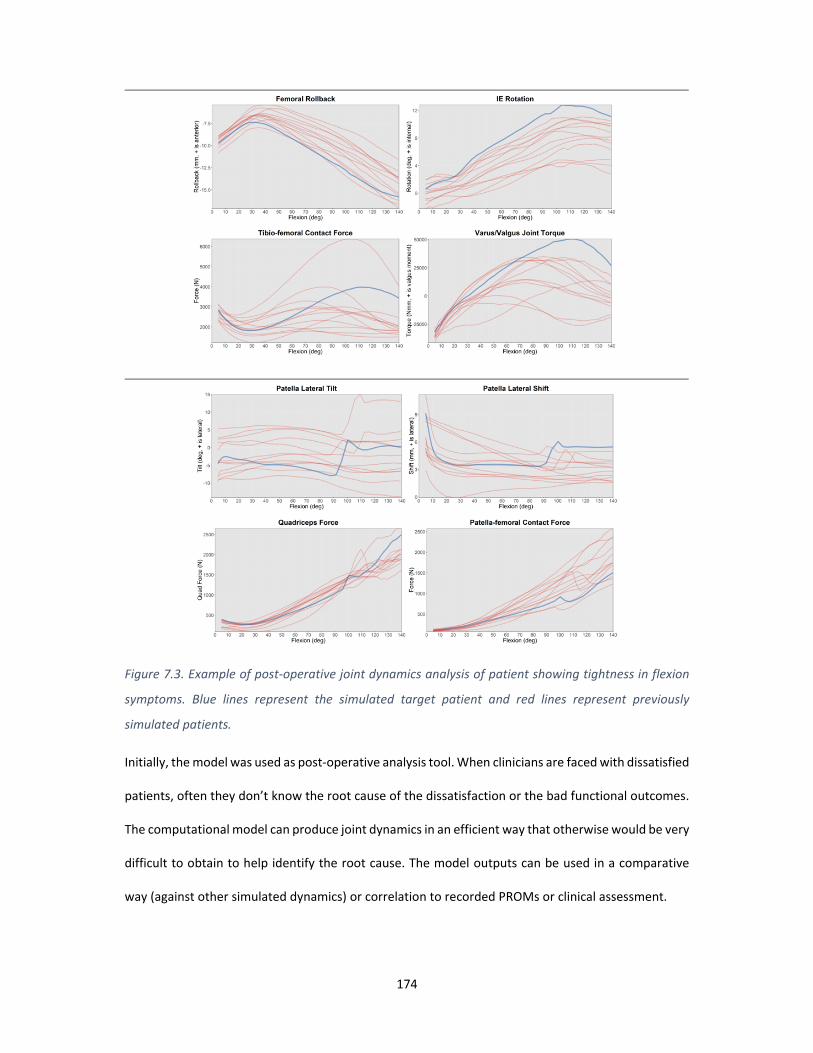
174

Figure 7.3. Example of post‐operative joint dynamics analysis of patient showing tightness in flexion

symptoms. Blue lines represent the simulated target patient and red lines represent previously

simulated patients.

Initially, the model was used as post‐operative analysis tool. When clinicians are faced with dissatisfied

patients, often they don’t know the root cause of the dissatisfaction or the bad functional outcomes.

The computational model can produce joint dynamics in an efficient way that otherwise would be very

difficult to obtain to help identify the root cause. The model outputs can be used in a comparative

way (against other simulated dynamics) or correlation to recorded PROMs or clinical assessment.

175

Figure 7.3 shows an example of a post‐operative dynamics analysis. From clinical assessment, patient

presented with tightness in flexion. The surgeon was uncertain what caused the tightness and

requested a dynamics analysis. From post‐operative CT, the implanted components were measured

as shown in the top picture. Both femur and tibia components were measured to be internally rotated,

but the coronal angle is within 3° relative to mechanical alignment. The computational model

predicted the tibia to be continuously internally rotated relative to the femur as flexion increases

resulting in higher tibio‐femoral IE mismatch. Consequently, higher varus‐valgus joint torque

difference is seen in flexion. The predicted dynamics also showed relatively higher tibio‐femoral

contact force compared to previously simulated patients, which is a surrogate measure of tightness in

the joint (resultant high reaction force between tibia and femur indicating joint is tight). This was in

accordance with the observed clinical assessment. Another observation was that the model showed a

sudden jump of patella tilt in deep flexion, indicating patella fell in the femoral groove which could be

due to the small size implants implanted. However, this observation was not seen clinically. Surgeon

used the simulated dynamics information as adjunct to what they observed clinically and finally

decided not to revise the patient as the potential gain vs effort of revising was not worthwhile. Instead,

they referred the patient to physiotherapy to improve the balance in flexion. If the surgeon was to

revise the knee, the model could also be used to model different tibia component alignment and

compare the resultant dynamics. In this analysis, only patient CT scan was used as inputs. Image

segmentation and landmarking was performed so that the computational model can be generated.

The surgeon’s clinical assessment was then compared to predicted dynamics outputs. This process

took approximately 3 hours (from CT segmentation to produce simulation results).

With sufficient number of post‐operative simulated dynamics and corresponding PROMs, correlation

between the dynamics characteristics that led to good outcomes as measured by PROMs could be

made. The correlation work is outside of this thesis main body. However, Twiggs et al [169], colleagues

at 360KneeSystems recently published a study where they found a few predicted dynamics

176

characteristics were significantly correlated to post‐operative PROMs. This work extends the

application of the current developed model further to pre‐operative context.

Figure 7.4 illustrates how computational modelling can be used pre‐operatively as part of surgical

planning. If we know which dynamics characteristics led to good clinical outcomes, the factors

affecting to the dynamics outcomes can be predicted. We know the patient specific anatomy from

imaging data, implant geometry from implant manufacturer and component alignment can be

virtually planned at different positions.

Figure 7.4. Illustration of application of computational model in surgical planning. If correlation of

dynamics outcome to clinical outcomes is known, i.e. what dynamics characteristics correlate to happy

patients, we can find the best component alignment to achieve the desired dynamics with

computational modelling given the known component geometry and patient specific anatomy factors.

One example of the application of the correlation found is to present the predicted dynamics

characteristics associated with post‐operative PROMs with a score using penalty function. This

summarises the predicted dynamics results in an easy interpretable format for clinicians. The score

represents whether the predicted dynamics is associated with good or bad post‐operative PROMS

based on the correlation analysis. Figure 7.5 shows an example of the application in pre‐operative

177

surgical planning. In this example, the tibia Internal‐External (IE) rotation and slope are iterated in the

computational model. Each corner of the plot represents a predicted dynamics result with specified

component position and geometry. The higher percentage score means the predicted dynamics is

associated with good post‐operative PROMs score and low score associated with bad post‐operative

PROMs. The score is highlighted with colour status (green associates with high percentage score while

red associates with low percentage score) so it is easily interpretable which component position and

geometry predicted dynamics result is associated with good and bad post‐operative PROMs.

Additionally, this analysis provides comparison of relative sensitivity of patient specific predicted

dynamics to component position and geometry. The right plots of Figure 7.5 shows the predicted

dynamics in each corner is associated with good post‐operative PROMs regardless of tibia component

position range and geometry selected. This implied the predicted dynamics of the specific patient is

not sensitive to tibia component position and geometry. Whereas, left plots of Figure 7.5 shows good

and bad post‐operative PROMs association. The plots show the predicted dynamics is associated with

good outcomes when the congruent tibial insert geometry is used and placed at high tibia slope. These

analyses are not intended to directly predict the patient’s post‐operative clinical outcome but as

adjunct information to surgeons so that they are better informed before the surgery and can make

appropriate assessment during surgery.

178

Figure 7.5. Predicted dynamics is presented as a score associated with post‐operative PROMs based on

the correlation analysis. The score is highlighted with colour status (green associates with high

percentage score while red associates with low percentage score). Left side plots show the predicted

dynamics is associated with good post‐operative PROMs when congruent tibia insert is used and placed

at high slope. Whereas the right‐side plots show the predicted dynamics in all selected tibia geometry

and position are associated with good post‐operative PROMs. These analyses are used as adjunct

information for surgeons to help them better plan the surgery and plan appropriate assessments for

implant selection.

Above example shows the variation of tibia component placement only. Occasionally, there are cases

where the predicted dynamics of all selected tibia component geometries and positions are associated

with bad post‐operative PROMs, i.e. red colour plots in all corners. In that instance, variations of the

femur component can be made to study which combination of femur, tibia and patella component

placement will result in good PROMs association. Surgeons are then better informed and can plan

appropriate assessments to make decision thoroughly intra‐operatively. There were examples where

the computational model results suggested to anteriorise the femur components by few millimetres

to reduce the tibio‐femoral tightness in flexion, which matched with surgeon findings intra‐

operatively.

Another application of studies conducted in this thesis was the attempt to predict the optimal femur

cuts to achieve joint gaps balance for gap balancing surgical technique. Quantification of 3D knee laxity

using technique described in Chapter 5 can provide more information to clinician pre‐operatively of

179

whether the knee is correctable to mechanical alignment. If the knee does not cross the neutral

mechanical alignment during varus‐valgus stress assessment, it is considered the knee is not

correctable and may need component alignment other than mechanical alignment to achieve balance.

Additionally, using the ligament parameters optimization technique described in Chapter 6, we can

measure the joint gaps of the knee under specific tension for gap balancing surgical technique. Gap

balancing require resecting the tibia bone first. Then, a tensioner is inserted to the joint to assess the

gaps in extension and flexion. The aim of the technique is to achieve equal gap in extension and flexion.

With the known ligament parameters to simulate the soft tissue tightness, the model can simulate

what femur cuts needed to achieve the joint gaps balance in extension and flexion. An example of the

concept report is shown in Figure 7.6.

Figure 7.6. A concept of ligament laxity report that utilises stress radiograph data to predict the joint

gaps for gap balancing surgical technique. The ligament parameters were optimized as per Chapter 6,

180

then used in a separate computational model to predict the optimal femur cuts to achieve a joint gap

balance in extension and flexion.

The knee computational model developed in this thesis has been used to analyse approximately 1,800

post‐operative CT’s. Meanwhile, the dynamic surgical planning has been provided for over 3,000 TKA.

This highlights the high utility of the model developed, with the capacity to simulate a large volume

cases in clinical setting. Undoubtably, not every single analysis had shown direct correlations to the

intra‐operative observation, but this is on‐going work. Part of the development work is data collection.

Patients are being followed up at 12 months for PROMs and post‐operative CT. This provides a

complete loop of data that bridges the pre‐operative, intra‐operative and post‐operative

environments. The data collected is a combination of physics, clinical and knowledge data; simulated

dynamics and PROMS or other clinical assessments. Overtime, this data may be the key to show a

reproducible relationship between joint dynamics and clinical outcomes.

Further application to help managing patient clinical outcomes

The continual collection of physics, clinical and knowledge data have large potential to develop a

successful patient centred care pathway. One extension from this study is to use Machine Learning to

further explore the correlations of joint dynamics and PROMs. Machine Learning techniques such as

supervised learning or un‐supervised learning can be used to study and learn the complex

relationships between soft tissue laxity, anatomical morphology, disease stage, joint dynamics and

PROMs. This will further enhance the current dynamics surgical planning.

Patient expectation is one of the key factors to the un‐met satisfaction [401]. Using similar concept,

Machine Learning can be used to predict patient satisfaction score based on their current pre‐

operative state and expectations. Further extension of physics and knowledge data is perhaps to

derive patient’s optimal dynamics characteristics based on their expectations (e.g. what activity they

would like to be able to do after TKA), and then plan the component position accordingly to achieve

181

the targeted dynamics. Then the desired dynamics is communicated to physiotherapist so that they

can tailor the rehabilitation program to support the patient’s needs.

Intra‐operative delivery technology also plays an important role in patient centred care pathway. The

surgeons need to be able to achieve the planned surgical plan. Use of Navigation system is increasing

in TKA procedures and is becoming more accessible to most hospitals. Ideally, surgical planning is

integrated with intra‐operative delivery technology so that if surgeon deviates from the initial plan,

the surgical planning tool can update the information and re‐calculate what component position

adjustments need to be made to still achieve the targeted joint dynamics, i.e. re‐run simulation in

intra‐operative setting. Current simulation takes few minutes to complete and one of the next

development pathways is to enable the model to complete a simulation under a minute. Further

application is to use Navigation system to collect the knee laxity data intra‐operatively and if the model

is efficient enough, ligament parameters optimization can be done at that time. Hence, it is important

to keep a balance of the model complexity so that it can be efficiently integrated to clinical setting.

This thesis started the focus in surgical planning in the patient centred care pathway and hopefully

can expand its application to other areas.

Use of Computational model as medical device

There are many developed knee computational models published in literature but not many of them

are used as medical device. This could be due to lack of guidance from regulatory bodies in how they

would assess software as a medical device, particularly software that provides in‐silico analysis.

Additionally, there are variations on regulatory requirements from different regulatory bodies, for

example Australia Therapeutic Goods Administration (TGA) accepts a medical device that has CE

marking while United States Food and Drug Administration (FDA) and Japan Pharmaceuticals and

Medical Devices Agency (PMDA) do not. Even though each regulatory body purpose is to control,

supervise and regulate medical devices, they have different specifics on their requirements. However,

182

regulatory bodies in the past few years have been aligning their requirements and moving towards

Medical Device Single Audit Program (MDSAP) which will allow medical device manufactures to be

audited once for compliance with the standard and regulatory requirements of up to five different

medical device markets: Australia, Brazil, Canada, Japan and the United States [416].

The other reason for lack of guidance is that medical devices traditionally have been mainly hardware

medical devices and regulatory safety and efficacy assessment is different from software devices.

There is software approved as medical devices but not many that are specific to computational

modelling technology. They are mainly used either in manufacturing or maintenance of a medical

device or software that resides in a medical device, e.g. Navigation system or Electromyograph

equipment. Hence, the assessment process for in‐silico software is vague. However recently, FDA in

collaboration with medical device developers, regulatory agencies and research institutions have

published new guidance to provide a framework to communicate computational modelling

verification and validation efforts. This guidance is published as “V&V 40 Verification and Validation

in Computational Modelling of Medical Devices” [417]. This guidance outlines recommendations on

key aspects of verification and validations steps so that the consistency and predictability of the

medical device review of computational modelling studies by FDA reviewers can be improved. The

guidance highlighted the first important factor is the “Context of Use” of the computational model.

The Context of Use sets the expectation on how the computational model is going to be used as well

as provide an overview for risks associated with the use. The level of credibility of the computational

model during verification and validation phase is then determined by the Context of Use and risks

identified. Overall, this is a good step from regulatory bodies to standardise the review process for in‐

silico software as medical device and this will enable the adoption of computational modelling as

medical device.

Realising TKA computational model for clinical use

183

The knee model developed and validated in Chapter 4 has obtained CE marking and TGA approval as

medical device. A brief summary on the process taken to achieve the regulatory approval will be

described. First, a medical device company need to have a Quality Management System (QMS) to

manufacture and distribute a medical device. Depending on the classification of the medical device,

there are different level of compliance on QMS needed. Typically, the QMS needs to comply with ISO

13485 standard, for CE marking and TGA, or 21 CFR Part 820 for FDA. In this case, 360 Knee systems

comply with ISO 13485. Then, the safety classification of the intended medical device was determined.

Based on the classification, level of documentation and testing is determined. For CE marking, a

checklist is used to scope the requirements needed to fulfil the regulatory bodies. The checklist is

called “Essential principal checklist”. The checklist outlines the areas the reviewer will assess, such as

verification, validation, requirements of the medical device, traceability between requirements and

testing, risk assessment and labelling. CE marking also require clinical evaluation to be performed to

ensure there is sufficient clinical evidence to confirm compliance with relevant essential requirements

for safety and performance of the device [418].

Within 360 Knee Systems, my role includes the computational model development and medical device

registration. I played a significant role in producing the documentation and evidence for the medical

device certification of the knee computational model. The software requirements and software design

specifications of the knee computational model was documented. Verification of the computational

model was conducted through cadaver lab experiment, as described in chapter 2, 3 and 4. Clinical

evaluation included surgeons’ expert feedback on the relevance of the predicted joint dynamics to

intra‐operative observation. Post‐operative data collection was also part of the clinical evaluation to

monitor the performance and relevance of the medical device. In summary, the main body of this

thesis was aimed at development of knee computational model as medical device as oppose to pure

research tool. Even though there are simplifications and limitations in the current model, the model

developed have been successfully gained approval and used as medical device and has the required

balance to be used as part of surgical planning.

184

As a thought exercise, what would be required to make changes to the current approved knee

computational model? For example, include a new implant system or simulate other activity or update

methodology used in creating the knee model. These changes can be categorised as minor and major

change.

For minor change, where no new risk introduced or context of use remains the same, technical

documents of the medical device, such as software requirements or software specifications need to

be updated for traceability purposes and testing need to be performed. Since it is minor change,

testing can be against benchmark cases to ensure the updated model produce same predicted

dynamics to the validated version. Benchmark cases can be the cadaver data used for validation. New

version release needs to be documented as part of QMS requirements. Re‐submission for regulatory

approval is not needed as no change in intended use and no new risk introduced.

For major change, where new significant risks are introduced or context of use is updated, the version

change involves more steps. Firstly, the new risks or updated context of use need to be identified and

assessed. These need to be assessed against the essential requirement checklist and any gaps need to

be determined introduced by the change request. Determine and document the new requirements

needed for the change. Testing coverage need to be assessed for the new requirements. If cadaver

testing is required because the current testing coverage is insufficient to cover the new functions or

features, define the scope of the new verification testing and reporting structure against V&V40

guidelines.

Re‐establish the verification and validation goals based on the updated context of use and risks. For

effective outcomes, ensure the testing is planned sufficiently. There are different levels of testing that

need to be performed. On the low level, software testing needs to be performed to ensure that new

features or functions introduced works as intended. Then, experimental testing such as cadaver

testing can be used to verify the computational model outputs. The cadaver testing needs to be

planned with suggestions described earlier. Finally, the updated model needs to be validated to ensure

185

outputs of the updated model are clinically relevant for its context of use. Clinical evaluation protocol

needs to be updated and ensure the reporting structure meets the regulatory requirements.

Once required testing for the proposed changes have been completed, documentation needs to be

updated for regulatory submission. Major change on registered medical device needs to be reported

to regulatory bodies in jurisdiction where the changes are going to be released on. For example,

regulatory body for CE mark will have to review the updated documentation and clinical evaluation.

For FDA, the reviewers will go through the change rationale to determine whether the medical device

is suitable for special 510k or require a new 510k application. Special 510k is a type of 510k application

that do not go through all review process as standard 510k process.

Concluding remarks

This thesis presented a series of studies towards the development of a low‐cost computational model

that aimed to be used as part of surgical planning tool to help clinicians triage patient treatments.

Consistent definitions of reference frames when validating a computational model need to be

emphasized to ensure no accuracy loss in data translation. Limitations were highlighted on the

validation steps but had outlined suggestions for future studies to avoid the mistakes that occurred.

Patient specific ligament characteristics were also shown to be important. Further work needs to

scope the validation of the optimization technique described and explore the combination effects of

patient specific ligament characteristics, implant geometry and component placements in the model.

The current model has been used as part of a medical device to compare the relative difference of

joint dynamics between patients. Regulatory bodies are catching up in this field and has recently

worked on standardizing verification and validation framework. Future work in realising

computational model as medical device need to align the development strategy against the guidance

to ensure successful regulatory application.

186

There are still a proportion of TKA patients who are dissatisfied. With increasing healthcare cost,

advances in patient centred care is important to help clinicians choose the best and most efficient

treatment plans for individual patient. This thesis started that journey with surgical planning that

utilises computational modelling technology to enhance patient outcomes.

187

Appendices

Appendix A ‐ First Computational Model Experimental Validation

Figure 2.7. Validation process of the developed computational model

10 Cadaveric knees (4 left/right pairs).

The knees were mounted in a dynamic, quadriceps‐driven, closed‐kinetic‐chain knee simulator based on the Oxford Knee Rig (OKR), as previously described in [276]. (See figure to

right)

TKR performed GMK components (Medacta, Switzerland).

Femoral, tibial and patella arrays were tracked by Stryker Navigation during closed‐kinetic‐

chain knee extension.

Fiducial markers (bone screws) attached to femur, tibia and patella and probed with

Stryker Navigation.

Post‐op CT used to build subject specific computational models (described in the

methods of the paper) with implants positions determined from CT by registering the implant

CAD models. (See figure on the left)

Experiment tibiofemoral and patellofemoral kinematics were compared to predicted model

kinematics.

Navigation arrays

Fiducial markers

Tibia component registration

Femur component registration

Navigation arrays attached to femur, tibia and patella (Stryker Navigation 4.0 Research Version, Kalamazoo, Michigan, US).

Segmented fiducials paired with probed fiducial points and used to virtually describe

the experimental tibiofemoral and patellofemoral movement during closed‐

kinetic‐chain knee extension.

188

Determination of Ligament stiffness

The stiffness coefficients of the PCL, LCL and MCL were initially adapted from previous studies [276].

They were then fined tuned so that the parameters can be used to achieve good correlations between

the experimental and predicted model kinematics for each cadaver subject. Tuned stiffness for

anterior MCL was 1.7 104 N, posterior MCL was 3.7 104 N, LCL was 6.4 104N, anterior PCL was 1.2

104 N and posterior PCL was 1.1 104 N.

Comparison of experimental and predicted model kinematics

For tibiofemoral kinematics, observations were made for tibiofemoral varus/valgus (Varus),

tibiofemoral axial rotation (IE Rotation), posterior translation of the mid‐point of the transepicondylar

line (Rollback), and medial and lateral flexion facet centre (FFC) where anterior position was relative

to the centre of the tibia plateau (Medial FFC AP & Lateral FFC AP). Correlations between the

experimental validation (test) and the simulation (model) for tibiofemoral kinematics are shown in

Figure 2.8 and the mean for each specimen, standard deviation and Pearson correlation coefficient (r)

are shown in Table 2.

189

(a) (b)

(c) (d)

(e)

Figure 2.8 Correlations for tibiofemoral kinematics (a) varus‐valgus; (b) IE rotation; (c) femoral

rollback; (d) medial FFC AP position; and (e) lateral FFC AP position

190

Table 2.1 Experimental validation and test mean (± standard deviation) and Pearson linear correlation

coefficient (r) for tibiofemoral kinematics

10° 45° 90°

Test Model r Test Model r Test Model r

Varus

‐2.01

± 2.51

‐2.30 ±

2.56 0.94

‐1.47

± 2.93

‐1.55 ±

2.95 0.99

0.05 ±

2.62

‐0.15 ±

2.46 0.97

IE Rotation

‐3.35

± 2.73

‐3.81 ±

3.74 0.76

‐2.49

± 2.15

‐3.11 ±

2.84 0.82

‐3.42 ±

4.34

‐3.27 ±

4.24 0.88

Rollback

‐6.82

± 2.64

‐7.51 ±

1.52 0.98

‐7.00

± 2.79

‐6.89 ±

2.05 0.88

‐8.29 ±

2.55

‐6.82 ±

2.86 0.95

Medial FFC

AP

‐7.17

± 3.56

‐8.10 ±

2.90 0.85

‐4.85

± 3.78

‐5.05 ±

3.43 0.96

‐4.31 ±

4.34

‐2.80 ±

4.10 0.97

Lateral FFC

AP

‐9.59

± 2.80

‐10.07

± 1.98 0.85

‐8.98

± 2.80

‐8.62 ±

1.95 0.73

‐8.23 ±

2.44

‐6.77 ±

2.40 0.88

For patellofemoral kinematics, observations were made for lateral translation of the patella (lateral

shift) and IE rotation about the patella centreline (patella tilt). Both measures were relative to a

coordinate system embedded in the femur. There were some linear trends for 10° and 45° however

less so for 90° particularly for patella tilt. Correlations between the experimental validation (test) and

the simulation (model) for patellofemoral kinematics are shown in Figure 2.9 and the mean for each

specimen, standard deviation and Pearson correlation coefficient (r) are shown in Table 2.2.

191

(a)

(b)

Figure 2.9 Correlations for patellofemoral kinematics (a) patella lateral shift and (b) patella tilt

Table 2.2. Experimental validation and test mean (± standard deviation) and Pearson linear correlation

coefficient (r) for patellofemoral kinematics

10° 45° 90°

Test Model r Test Model r Test Model r

Patella lateral

shift

3.16 ±

2.59

2.99 ±

2.01

0.95 1.82 ±

2.68

1.68 ±

1.82

0.93 2.71 ±

3.65

1.80 ±

1.93

0.67

Patella tilt 5.49 ±

6.33

5.87 ±

3.29

0.79 9.63 ±

6.13

6.97 ±

3.64

0.87 5.89 ±

5.87

3.73 ±

2.74

0.38

192

Appendix B ‐ Verification of 3D‐2D Registration technique using

Sawbone Model

In order to determine the accuracy of described 3D‐2D registration and the methods used to calculate

knee alignment, a sawbone model was constructed to allow manipulation to specific flexion angle.

The model contains full length of the femur, tibia and fibula, interconnected by 4 stretchable ligaments

representing the anterior & posterior cruciate ligaments and the medial & lateral collateral ligaments.

The sawbone was taken for CT scan and segmentation and landmarking was performed on the scan.

The sawbone chosen for the purpose of this study is made up on two types of material – a dense foam

shell to represent the cortical bone and a highly porous interconnected structure to represent the

cancellous bone. While the density of these materials is significantly lower than that of human bone,

the density of the sawbone model is sufficient to visible under x‐ray.

A mechanical frame was constructed to hold the sawbone model at specific flexion angle. 6mm holes

were drilled into the dense, cortical and porous, cancellous bones, a steel nut is inserted through to

lock the 6 degrees of freedom, see Figure 5.9. Mechanical frame constructed to hold the sawbone at

different flexion anglesError! Reference source not found.. Holes are drilled into both the fixation rig

and the sawbone model in order to achieve the following positions:

Extension

Midflexion

Flexion (90°)

193

Figure 5.9. Mechanical frame constructed to hold the sawbone at different flexion angles

The sawbone was then taken for lateral and anterior‐posterior (AP) X‐ray for each of the flexion

position. Figure 5.10. Example of AP and lateral X‐ray taken for sawbone model at 90° flexion. shows

example of when the sawbone’s X‐ray was taken.

Figure 5.10. Example of AP and lateral X‐ray taken for sawbone model at 90° flexion.

3D‐2D registration technique described in Method section was performed to determine the knee

alignment of the sawbone position. Figure 5.11 shows the 3D‐2D registration screenshots.

A handheld 3D scanner, HandyScan (Creaform Inc, Quebec, Canada) was used to capture the surface

geometry of the sawbone at each specified flexion angle. Output of this scan was 3D model of the

194

femur and tibia in space. A resolution of 0.6mm is used in the scanning process. With the sawbone in

place, the anterior and posterior surfaces of the bones cannot be captured in a single scan. Thus,

multiple scans are taken so that the anterior and posterior surfaces can be stitched to form a 3D model

using processing software part of the handheld device, VX elements (Creaform Inc, Quebec, Canada).

Figure 5.12 shows an example of the scanning and stitching process of the handheld device.

Segmented CT scan 3D model was aligned to the generated 3D surface model of the sawbone at each

specified flexion position using Iterative Closest Point (ICP) alignment method in Powershape

(Autodesk, California, United States). The knee alignment of this registration is considered to be the

benchmark because surface‐to‐surface registration is more deterministic than 3D‐2D registration

method, especially when the surface compared are identical. Following similar steps described in

Method section, once the CT bone models were registered to scanned position, the landmarks

determined from CT were transformed using the bone models’ transformation matrix. The knee

alignment is then described using Grood and Suntay convention.

Knee alignment derived using 3D‐2D registration technique was compared to the knee alignment

derived using surface‐to‐surface registration.

195

ExtensionAP Mid‐FlexionAP FlexionAP

Extension Lateral Mid‐Flexion Lateral Flexion Lateral

Figure 5.11. screenshots of 3D‐2D registration of the sawbone at each flexion angle for AP and lateral

X‐ray.

196

Figure 5.12. HandyScan captured surface geometry of femur. Left and centre: Align tool in VX Elements

to stich two meshes together. Right: merged mesh showing missing features and surfaces filled.

Results

Verification of 3D‐2D registration techniques was conducted by comparing data obtained from 3D

scans with alignment calculations from geometry registered using 3D‐2D x‐ray registration.

Table 5.4: Alignment information calculated from 3D scan in fixed positions.

Table 5.5: Alignment information calculated from X‐ray registration of both anterior posterior (AP) and

lateral x‐rays.

Position FE VV IE ML AP SI

Extension 2.4 6.7 0.8 5.5 12.3 ‐43.1

Flexion 101.6 4.3 ‐3.1 7.4 14.5 ‐43.0

Mid‐Flexion 67.9 7.9 ‐7.3 1.6 13.9 ‐43.8

Position Direction of X‐ray FE VV IE ML AP SI

Extension AP 4.2 7.1 2.0 6.9 18.4 ‐42.7

Lateral 2.8 6.6 1.9 5.8 12.6 ‐43.3

Flexion AP 104.9 4.2 ‐2.0 7.6 12.0 ‐44.8

Lateral 101.6 4.6 ‐2.5 5.0 13.5 ‐43.8

Mid‐

Flexion

AP 64.4 7.2 ‐6.7 1.4 12.8 ‐43.8

Lateral 67.7 7.3 ‐7.0 4.3 14.4 ‐43.6

197

Table 5.6: Comparison of the 6 degrees of freedom in terms of alignment between the 3D scan method

and the x‐ray registration method.

Figure 5.13. Verification of the 3D‐2D Registration and post‐processing

From Table 5.6Table 5. and Figure 5.1, it can be seen that the greatest variation in all x‐rays is the

anterior and posterior position in the Extension AP X‐ray. AP X‐rays showed the greatest deviation in

the anterior‐posterior direction and lateral x‐rays showed the greatest deviation in the medial lateral

direction.

0.0

0.5

1.0

1.5

2.0

2.5

Difference in alignmen

t calculation

Extension Flexion Mid Flexion

Mean Accuracy of X‐ray Registration

AP

Lateral

Differences FE VV IE ML AP SI

Extension_AP 1.8 0.4 1.2 1.4 6.1 0.5

Extension_L 0.4 0.1 1.1 0.3 0.2 0.2

Flexion_AP 3.4 0.2 1.1 0.2 2.5 1.8

Flexion_L 0.1 0.3 0.6 2.4 1.0 0.8

MidFlexion_AP 3.5 0.7 0.6 0.2 1.1 0.0

MidFlexion_L 0.2 0.6 0.4 2.7 0.5 0.2

Average 1.6 0.4 0.8 1.2 1.9 0.6

Average exclude AP Xrays

0.2 0.3 0.7 1.8 0.6 0.4

198

It was anticipated that the greatest degree of variation will be the translational degree of freedom

that is perpendicular to the x‐ray plate (in and out‐plane). i.e. for AP x‐rays, translation in the AP

direction will be the most difficult to define. The difference in translation about this axis is subjective

given that the effects of magnification do not clearly show even when the geometry is translated by

several millimetres towards or away from the x‐ray. Largest difference in registered AP X‐ray was

6.4mm for AP position and for lateral X‐ray was 2.7mm for ML position.

This study showed that the overall accuracy for method described (both types of x‐rays). AP Xrays

were found to be less accurate for flexion angle and AP measurements due to the out‐of‐plane motion.

Only lateral AP Xrays were used in this study and when AP Xrays were excluded, the accuracy of this

method was 0.6mm for in‐plane translation, 1.8mm for out‐of‐plane translation and 0.7° for rotations.

The relative registered position between femur and tibia need to be reviewed closely for absurdity to

minimise in‐plane translational distance error.

199

Appendix C – Validation of ScanIP Software Measurements

As described in Chapter 3, ScanIP is an FDA approved medical software specifically designed to process

medical imaging and registration of 3D models. It is important to ensure the software outputs are

correct in order to interpret the analysis accurately. The test protocol and report described below is

part of 360KneeSystems technical file for their surgical planning medical device. Permissions have

been granted by 360KneeSystems to only describe the protocol and report as summary.

Test Protocol

A CT calibration phantom with known geometry was used in the test. The calibration phantom

contains radiopaque screws at specified location with known measurements. Figure 13.7 below shows

the calibration phantom engineering drawings with known measurements. The physical calibration

phantom was sent to 3 different radiology centres to be CT scanned. The CT scan of the calibration

phantom from each centre was segmented and landmarked using ScanIP. Figure 3.8 shows an example

of the segmented and landmarked calibration phantom screws. The landmarked measurements were

then compared to the engineering drawings for comparison. The acceptance criteria of the ScanIP

outputs is to be within 1mm and 0.7° from the reference measurements.

200

Figure 13.7. Engineering drawing of CT calibration phantom used to validate ScanIP software measurements.

Figure 3.814. Example of the segmented and landmarked calibration phantom

201

Results

Measurement deviations of processed CT calibration phantom scanned at each radiology centre were

shown in Figure 3.9 and Figure 3.10. As can be seen from the graphs, all measurements from ScanIP

were under the set maximum acceptance level and therefore we can be confident that ScanIP

measurement outputs are reliable.

Figure 3.9. Distance measurements deviation between processed CT calibration phantom against engineering drawing. All measurements are within acceptance criteria (1mm).

0

0.1

0.2

0.3

0.4

0.5

0.6

0.7

0.8

0.9

1

1.1

1.2

0 5 10 15 20 25

Deviation From eng. drawing (m

m)

Observation Number

CT Scanner Models & Measurements ‐ (mm)

Mater Imaging PRP Dee Why Castlereagh Imaging

Maximum Acceptance Level

202

Figure 3.1015. Angular measurements deviation between processed CT calibration phantom against engineering drawing. All measurements are within acceptance criteria (0.7°).

0

0.1

0.2

0.3

0.4

0.5

0.6

0.7

0.8

0 1 2 3 4 5 6Deviation From Laser Scan

(degrees)

Observation Number

CT Scanner Models & Measurements ‐degrees

Mater Imaging PRP Dee Why Castlereagh Imaging

Maximum Acceptance Level

203

References

[1] "National Joint Replacement Registry Annual Report," Australian Orthopaedic Association,Adelaide2017.

[2] R. B. Bourne, B. M. Chesworth, A. M. Davis, N. N. Mahomed, and K. D. J. Charron, "Patientsatisfaction after total knee arthroplasty: Who is satisfied and who is not?," ClinicalOrthopaedics and Related Research, 2010.

[3] W. Muller, The Knee ‐ Form, Function, and Ligament Reconstruction. Springer, 1982.[4] G. R. T. Scuderi, A. J., The Knee. SG: World Scientific, 2010.[5] H. Gray, Anatomy of the Human body 20th edition. Philadelphia: Lea & Febiger, 1918.[6] A. M. Amendola, S.; Menetrey, J.; Bellemans, J., The Knee Joint: Surgical Techniques and

Strategies. Springer, 2012.[7] E. Thienpont, Improving Accuracy in Knee Arthroplasty. New Delhi: Jaypee, 2012.[8] E. Y. Chao, E. V. Neluheni, R. W. Hsu, and D. Paley, "Biomechanics of malalignment," Orthop

Clin North Am, vol. 25, no. 3, pp. 379‐386, 1994.[9] D. Paley, J. E. Herzenberg, K. Tetsworth, J. McKie, and A. Bhave, "Deformity planning for frontal

and sagittal plane corrective osteotomies," Orthop Clin North Am, vol. 25, no. 3, pp. 425‐465,1994.

[10] J. Bellemans, W. Colyn, H. Vandenneucker, and J. Victor, "The Chitranjan Ranawat award: isneutral mechanical alignment normal for all patients? The concept of constitutional varus,"Clinical orthopaedics and related research, vol. 470, no. 1, pp. 45‐53, 2012.

[11] A. Escalante, M. J. Lichtenstein, R. Dhanda, J. E. Cornell, and H. P. Hazuda, "Determinants ofhip and knee flexion range: results from the San Antonio Longitudinal Study of Aging," (in eng),Arthritis Care Res, vol. 12, no. 1, pp. 8‐18, 1999.

[12] K. E. Roach and T. P. Miles, "Normal hip and knee active range of motion: the relationship toage," (in eng), Physical Therapy, vol. 71, no. 9, pp. 656‐665, 1991.

[13] M. A. Strickland, M. Browne, and M. Taylor, "Could passive knee laxity be related to active gaitmechanics? An exploratory computational biomechanical study using probabilistic methods,"Computer Methods in Biomechanics and Biomedical Engineering, vol. 12, no. 6, pp. 709‐720,2009.

[14] L. G. Hallen and O. Lindahl, "The "screw‐home" movement in the knee‐joint," (in eng), ActaOrthop Scand, vol. 37, no. 1, pp. 97‐106, 1966.

[15] V. Pinskerova et al., "Does the femur roll‐back with flexion?," J Bone Joint Surg Br, vol. 86, no.6, pp. 925‐931, 2004.

[16] S. A. Banks, G. D. Markovich, and W. A. Hodge, "In vivo kinematics of cruciate‐retaining and ‐substituting knee arthroplasties," (in eng), J Arthroplasty, vol. 12, no. 3, pp. 297‐304, 1997.

[17] J. B. Stiehl, D. A. Dennis, R. D. Komistek, and H. S. Crane, "In vivo determination of condylarlift‐off and screw‐home in a mobile‐bearing total knee arthroplasty," (in eng), J Arthroplasty,vol. 14, no. 3, pp. 293‐299, 1999.

[18] D. A. Dennis, R. D. Komistek, J. B. Stiehl, S. A. Walker, and K. N. Dennis, "Range of motion aftertotal knee arthroplasty. The effect of implant design and weight‐bearing conditions," Journalof Arthroplasty, vol. 13, pp. 748‐752, 1998.

[19] C. W. Clary, C. K. Fitzpatrick, L. P. Maletsky, and P. J. Rullkoetter, "The influence of total kneearthroplasty geometry on mid‐flexion stability: an experimental and finite element study," (ineng), J Biomech, vol. 46, no. 7, pp. 1351‐7, Apr 26 2013.

[20] G. Yildirim, P. S. Walker, and J. Boyer, "Total knees designed for normal kinematics evaluatedin an up‐and‐down crouching machine," (in eng), J Orthop Res, vol. 27, no. 8, pp. 1022‐7, Aug2009.

[21] R. Shenoy, P. S. Pastides, and D. Nathwani, "(iii) Biomechanics of the knee and TKR,"Orthopaedics and Trauma, vol. 27, no. 6, pp. 364‐371, 2013.

204

[22] M. A. R. Freeman and V. Pinskerova, "The movement of the normal tibio‐femoral joint," (in eng), Journal of Biomechanics, vol. 38, no. 2, pp. 197‐208, 2005.

[23] J. Victor, L. Labey, P. Wong, B. Innocenti, and J. Bellemans, "The influence of muscle load on tibiofemoral knee kinematics," (in eng), J Orthop Res, vol. 28, no. 4, pp. 419‐28, Apr 2010.

[24] H. Iwaki, V. Pinskerova, and M. A. Freeman, "Tibiofemoral movement 1: the shapes and relative movements of the femur and tibia in the unloaded cadaver knee," (in eng), J Bone Joint Surg Br, vol. 82, no. 8, pp. 1189‐95, Nov 2000.

[25] J. S. Li, A. Hosseini, L. Cancre, N. Ryan, H. E. Rubash, and G. Li, "Kinematic characteristics of the tibiofemoral joint during a step‐up activity," (in eng), Gait Posture, vol. 38, no. 4, pp. 712‐6, Sep 2013.

[26] E. Most, J. Axe, H. Rubash, and G. Li, "Sensitivity of the knee joint kinematics calculation to selection of flexion axes," (in eng), J Biomech, vol. 37, no. 11, pp. 1743‐8, Nov 2004.

[27] E. S. Grood and W. J. Suntay, "A joint coordinate system for the clinical description of three‐dimensional motions: application to the knee," J Biomech Eng, vol. 105, no. 2, pp. 136‐144, 1983.

[28] B. J. Fregly, W. G. Sawyer, M. K. Harman, and S. A. Banks, "Computational wear prediction of a total knee replacement from in vivo kinematics," J Biomech, vol. 38, no. 2, pp. 305‐314, 2005.

[29] J. Morrison, "The mechanics of the knee joint in relation to normal walking," Journal of Biomechanics, vol. 3, pp. 51‐61, 1970.

[30] T. P. Andriacchi, G. B. Andersson, R. W. Fermier, D. Stern, and J. O. Galante, "A study of lower‐limb mechanics during stair‐climbing," (in eng), Journal of Bone and Joint Surgery [Am], vol. 62, no. 5, pp. 749‐757, 1980.

[31] G. Bergmann, F. Graichen, and A. Rohlmann, "Hip joint loading during walking and running, measured in two patients," (in eng), J Biomech, vol. 26, no. 8, pp. 969‐990, 1993.

[32] S. J. G. Taylor, J. S. Perry, J. M. Meswania, N. Donaldson, P. S. Walker, and S. R. Cannon, "Telemetry of forces from proximal femoral replacements and relevance to fixation," Journal of Biomechanics, vol. 30, pp. 225‐234, 1997.

[33] S. J. Taylor and P. S. Walker, "Forces and moments telemetered from two distal femoral replacements during various activities," J Biomech, vol. 34, no. 7, pp. 839‐848, 2001.

[34] K. R. Kaufman, N. Kovacevic, S. E. Irby, and C. W. Colwell, "Instrumented implant for measuring tibiofemoral forces," J Biomech, vol. 29, no. 5, pp. 667‐671, 1996.

[35] I. Kutzner et al., "Loading of the knee joint during activities of daily living measured in vivo in five subjects," Journal of Biomechanics, vol. 43, no. 11, pp. 2164‐2173, 2010.

[36] D. D. D'Lima, S. Patil, N. Steklov, S. Chien, and Colwell C.W, Jr., "In vivo knee moments and shear after total knee arthroplasty," Journal of Biomechanics, vol. 40, pp. S11‐S17, 2007.

[37] D. D. D'Lima, S. Patil, N. Steklov, J. E. Slamin, and C. W. Colwell Jr, "Tibial forces measured in vivo after total knee arthroplasty," J Arthroplasty, vol. 21, no. 2, pp. 255‐262, 2006.

[38] D. T. Reilly and M. Martens, "Experimental Analysis of the Quadriceps Muscle Force and Patello‐Femoral Joint Reaction Force for Various Activities," Acta Orthopaedica Scandinavica, vol. 43, no. 2, pp. 126‐137, 1972/01/01 1972.

[39] K. B. Shelburne, M. R. Torry, and M. G. Pandy, "Muscle, ligament, and joint‐contact forces at the knee during walking," (in eng), Med Sci Sports Exerc, vol. 37, no. 11, pp. 1948‐56, Nov 2005.

[40] D. E. Toutoungi, T. W. Lu, A. Leardini, F. Catani, and J. J. O'Connor, "Cruciate ligament forces in the human knee during rehabilitation exercises," (in eng), Clin Biomech (Bristol, Avon), vol. 15, no. 3, pp. 176‐87, Mar 2000.

[41] J. M. B. Jacquelin Perry, "Gait Analysis: Normal and Pathological Function," Journal of Sports Science & Medicine, vol. 9, no. 2, pp. 353‐353, 2010.

[42] "Kinematics of the knee during gait." [43] W. R. Taylor, M. O. Heller, G. Bergmann, and G. N. Duda, "Tibio‐femoral loading during human

gait and stair climbing," J Orthop Res, vol. 22, no. 3, pp. 625‐632, 2004.

205

[44] P. A. Costigan, K. J. Deluzio, and U. P. Wyss, "Knee and hip kinetics during normal stair climbing," Gait & Posture, vol. 16, no. 1, pp. 31‐37, 2002.

[45] V. Pinskerova, K. M. Samuelson, J. Stammers, K. Maruthainar, A. Sosna, and M. A. Freeman, "The knee in full flexion: an anatomical study," J Bone Joint Surg Br, vol. 91, no. 6, pp. 830‐834, 2009.

[46] M. A. R. Freeman and V. Pinskerova, "The movement of the knee studied by magnetic resonance imaging," (in eng), Clinical Orthopaedics and Related Research, no. 410, pp. 35‐43, 2003.

[47] K. M. Varadarajan, R. E. Harry, T. Johnson, and G. Li, "Can in vitro systems capture the characteristic differences between the flexion‐extension kinematics of the healthy and TKA knee?," Med Eng Phys, vol. 31, no. 8, pp. 899‐906, 2009.

[48] G. Li, T. W. Rudy, M. Sakane, A. Kanamori, C. B. Ma, and S. L. Woo, "The importance of quadriceps and hamstring muscle loading on knee kinematics and in‐situ forces in the ACL," (in eng), J Biomech, vol. 32, no. 4, pp. 395‐400, Apr 1999.

[49] M. L. Zimny, M. Schutte, and E. Dabezies, "Mechanoreceptors in the human anterior cruciate ligament," (in eng), Anat Rec, vol. 214, no. 2, pp. 204‐9, Feb 1986.

[50] R. A. Schultz, D. C. Miller, C. S. Kerr, and L. Micheli, "Mechanoreceptors in human cruciate ligaments. A histological study," (in eng), J Bone Joint Surg Am, vol. 66, no. 7, pp. 1072‐6, Sep 1984.

[51] M. J. Schutte, E. J. Dabezies, M. L. Zimny, and L. T. Happel, "Neural anatomy of the human anterior cruciate ligament," (in eng), J Bone Joint Surg Am, vol. 69, no. 2, pp. 243‐7, Feb 1987.

[52] Z. Halata, C. Wagner, and K. I. Baumann, "Sensory nerve endings in the anterior cruciate ligament (Lig. cruciatum anterius) of sheep," (in eng), Anat Rec, vol. 254, no. 1, pp. 13‐21, Jan 1999.

[53] B. Fromm and W. Kummer, "Nerve supply of anterior cruciate ligaments and of cryopreserved anterior cruciate ligament allografts: a new method for the differentiation of the nervous tissues," (in eng), Knee Surg Sports Traumatol Arthrosc, vol. 2, no. 2, pp. 118‐22, 1994.

[54] G. Limbert, "Finite element modelling of biological connective soft tissues: Applications to the ligaments of the human knee," University of Southampton, 2001.

[55] A. Viidik, "A rheological model for uncalcified parallel‐fibred collagenous tissue," (in eng), J Biomech, vol. 1, no. 1, pp. 3‐11, 1968.

[56] M. Abrahams, "Mechanical behavior of tendon in vitro," Medical & Biological Engineering, vol. 5, no. 433, 1967.

[57] E. S. Butler Grood and F. R. D. L. Noyes, "Biomechanics of ligaments and tendons," Exercise and Sport Sciences Reviews, vol. 6: 125, 1978.

[58] T. J. Momersteeg, L. Blankevoort, R. Huiskes, J. G. Kooloos, J. M. Kauer, and J. C. Hendriks, "The effect of variable relative insertion orientation of human knee bone‐ligament‐bone complexes on the tensile stiffness," (in eng), Journal of Biomechanics, vol. 28, no. 6, pp. 745‐752, 1995.

[59] T. J. Mommersteeg, L. Blankevoort, R. Huiskes, J. G. Kooloos, and J. M. Kauer, "Characterization of the mechanical behavior of human knee ligaments: a numerical‐experimental approach," J Biomech, vol. 29, no. 2, pp. 151‐160, 1996.

[60] P. S. Trent, P. S. Walker, and B. Wolf, "Ligament length patterns, strength, and rotational axes of the knee joint," (in eng), Clin Orthop Relat Res, no. 117, pp. 263‐70, Jun 1976.

[61] J. Wismans, F. Veldpaus, J. Janssen, A. Huson, and P. Struben, "A three‐dimensional mathematical model of the knee‐joint," Journal of Biomechanics, vol. 13, pp. 9‐9.

[62] L. Blankevoort and R. Huiskes, "Ligament‐bone interaction in a three‐dimensional model of the knee," J Biomech Eng, vol. 113, no. 3, pp. 263‐269, 1991.

[63] D. L. Butler, E. S. Grood, F. R. Noyes, R. F. Zernicke, and K. Brackett, "Effects of structure and strain measurement technique on the material properties of young human tendons and fascia," (in eng), J Biomech, vol. 17, no. 8, pp. 579‐96, 1984.

206

[64] A. Race and A. A. Amis, "The mechanical properties of the two bundles of the human posterior cruciate ligament," J Biomech, vol. 27, no. 1, pp. 13‐24, 1994.

[65] M. Freutel, H. Schmidt, L. Durselen, A. Ignatius, and F. Galbusera, "Finite element modeling of soft tissues: material models, tissue interaction and challenges," (in eng), Clin Biomech (Bristol, Avon), vol. 29, no. 4, pp. 363‐72, Apr 2014.

[66] H. Naghibi Beidokhti, D. Janssen, S. van de Groes, J. Hazrati, T. Van den Boogaard, and N. Verdonschot, "The influence of ligament modelling strategies on the predictive capability of finite element models of the human knee joint," J Biomech, vol. 65, pp. 1‐11, Dec 8 2017.

[67] F. Galbusera et al., "Material models and properties in the finite element analysis of knee ligaments: a literature review," Front Bioeng Biotechnol, vol. 2, p. 54, 2014.

[68] E. M. Abdel‐Rahman and M. S. Hefzy, "Three‐dimensional dynamic behaviour of the human knee joint under impact loading," Medical Engineering & Physics, vol. 20, no. 4, pp. 276‐290, 1998.

[69] V. K. Srikanth, J. L. Fryer, G. Zhai, T. M. Winzenberg, D. Hosmer, and G. Jones, "A meta‐analysis of sex differences prevalence, incidence and severity of osteoarthritis," (in eng), Osteoarthritis Cartilage, vol. 13, no. 9, pp. 769‐81, Sep 2005.

[70] V. Silverwood, M. Blagojevic‐Bucknall, C. Jinks, J. L. Jordan, J. Protheroe, and K. P. Jordan, "Current evidence on risk factors for knee osteoarthritis in older adults: a systematic review and meta‐analysis," (in eng), Osteoarthritis Cartilage, vol. 23, no. 4, pp. 507‐15, Apr 2015.

[71] J. A. C. van Tunen et al., "Association of osteoarthritis risk factors with knee and hip pain in a population‐based sample of 29‐59 year olds in Denmark: a cross‐sectional analysis," (in eng), BMC Musculoskelet Disord, vol. 19, no. 1, p. 300, Aug 21 2018.

[72] P. Suri, D. C. Morgenroth, and D. J. Hunter, "Epidemiology of osteoarthritis and associated comorbidities," (in eng), Pm r, vol. 4, no. 5 Suppl, pp. S10‐9, 2012.

[73] J. R. Bellemans, Michael D; Victor, Jan M.K., Total Knee Arthroplasty, 1 ed. (A Guide to Get Better Performance). Springer‐Verlag Berlin Heidelberg, 2005.

[74] "Swedish Knee Arthoplasty Register: Annual Report 2008," Department of Orthopaedics, University Hospital in Lund, Sweden2008, Available: http://internal‐pdf//Swedish knee arthroplasty report 2008Engl_1.1‐2509343488/Swedish knee arthroplasty report 2008Engl_1.1.pdf.

[75] M. J. Walton, A. E. Weale, and J. H. Newman, "The progression of arthritis following lateral unicompartmental knee replacement," The Knee, vol. 13, no. 5, pp. 374‐377, 2006.

[76] P. V. Papas, F. D. Cushner, and G. R. Scuderi, "The History of Total Knee Arthroplasty," Techniques in Orthopaedics, vol. 33, no. 1, pp. 2‐6, 2018.

[77] U. N. J. Registry, "National Joint Registry for England, Wales, Northern Ireland and the Isle of Man," 2018.

[78] L. University, "Swedish Knee Arthroplasty Registry," 2018. [79] B. C. Carr and T. Goswami, "Knee implants ‐ Review of models and biomechanics," Materials

& Design, vol. 30, no. 2, pp. 398‐413, 2009. [80] P. Ducheyne, A. Kagan 2nd, and J. A. Lacey, "Failure of total knee arthroplasty due to loosening

and deformation of the tibial component," (in eng), J Bone Joint Surg Am, vol. 60, no. 3, pp. 384‐391, 1978.

[81] S. M. Kurtz, H. A. Gawel, and J. D. Patel, "History and systematic review of wear and osteolysis outcomes for first‐generation highly crosslinked polyethylene," (in eng), Clin Orthop Relat Res, vol. 469, no. 8, pp. 2262‐2277, 2011.

[82] D. D. D. T. L. Amendola M. Fosco, "History of Condylar Total Knee Arthroplasty," Interchopen, 2012.

[83] S. D. Reinitz, B. H. Currier, D. W. Van Citters, R. A. Levine, and J. P. Collier, "Oxidation and other property changes of retrieved sequentially annealed UHMWPE acetabular and tibial bearings," J Biomed Mater Res B Appl Biomater, 2014.

207

[84] S. Joglekar, T. J. Gioe, P. Yoon, and M. H. Schwartz, "Gait analysis comparison of cruciateretaining and substituting TKA following PCL sacrifice," (in eng), Knee, vol. 19, no. 4, pp. 279‐85, Aug 2012.

[85] B. S. Parsley, M. A. Conditt, R. Bertolusso, and P. C. Noble, "Posterior cruciate ligamentsubstitution is not essential for excellent postoperative outcomes in total knee arthroplasty,"(in eng), J Arthroplasty, vol. 21, no. 6 Suppl 2, pp. 127‐31, Sep 2006.

[86] C. L. Peters, P. Mulkey, J. Erickson, M. B. Anderson, and C. E. Pelt, "Comparison of total kneearthroplasty with highly congruent anterior‐stabilized bearings versus a cruciate‐retainingdesign," (in eng), Clin Orthop Relat Res, vol. 472, no. 1, pp. 175‐80, Jan 2014.

[87] U. G. Longo et al., "Outcomes of Posterior‐Stabilized Compared with Cruciate‐Retaining TotalKnee Arthroplasty," (in eng), J Knee Surg, vol. 31, no. 4, pp. 321‐340, Apr 2018.

[88] M. S. Kuster and G. W. Stachowiak, "Factors affecting polyethylene wear in total kneearthroplasty," (in eng), Orthopedics, vol. 25, no. 2 Suppl, pp. s235‐42, 2002.

[89] Y. H. Kim, S. H. Yoon, and J. S. Kim, "The long‐term results of simultaneous fixed‐bearing andmobile‐bearing total knee replacements performed in the same patient," (in eng), J Bone JointSurg Br, vol. 89, no. 10, pp. 1317‐1323, 2007.

[90] M. W. Pagnano and R. M. Menghini, "Rotating platform knees: an emerging clinical standard:in opposition," (in eng), J Arthroplasty, vol. 21, no. 4 Suppl 1, pp. 37‐39, 2006.

[91] C. L. Barnes, J. D. Blaha, D. DeBoer, P. Stemniski, R. Obert, and M. Carroll, "Assessment of amedial pivot total knee arthroplasty design in a cadaveric knee extension test model," JArthroplasty, vol. 27, no. 8, pp. 1460‐1468 e1, 2012.

[92] J. D. Blaha, "A medial pivot geometry," (in eng), Orthopedics, vol. 25, no. 9, pp. 963‐964, 2002.[93] A. M. Hollister, S. Jatana, A. K. Singh, W. W. Sullivan, and A. G. Lupichuk, "The axes of rotation

of the knee," (in eng), Clin Orthop Relat Res, no. 290, pp. 259‐268, 1993.[94] N. Shimizu, T. Tomita, T. Yamazaki, H. Yoshikawa, and K. Sugamoto, "In Vivo Movement of

Femoral Flexion Axis of a Single‐Radius Total Knee Arthroplasty," J Arthroplasty, 2013.[95] A. R. Jo, E. K. Song, K. B. Lee, H. Y. Seo, S. K. Kim, and J. K. Seon, "A Comparison of Stability and

Clinical Outcomes in Single‐Radius Versus Multi‐Radius Femoral Design for Total KneeArthroplasty," J Arthroplasty, 2014.

[96] J. Palmer, K. Sloan, and G. Clark, "Functional outcomes comparing Triathlon versus Duracontotal knee arthroplasty: does the Triathlon outperform its predecessor?," Int Orthop, vol. 38,no. 7, pp. 1375‐1378, 2014.

[97] S. Ostermeier and C. Stukenborg‐Colsman, "Quadriceps force after TKA with femoral singleradius," (in eng), Acta Orthop, vol. 82, no. 3, pp. 339‐343, 2011.

[98] H. Wang, K. J. Simpson, M. S. Ferrara, S. Chamnongkich, T. Kinsey, and O. M. Mahoney,"Biomechanical differences exhibited during sit‐to‐stand between total knee arthroplastydesigns of varying radii," (in eng), J Arthroplasty, vol. 21, no. 8, pp. 1193‐1199, 2006.

[99] J. E. Stoddard, D. J. Deehan, A. M. Bull, A. W. McCaskie, and A. A. Amis, "The kinematics andstability of single‐radius versus multi‐radius femoral components related to mid‐rangeinstability after TKA," J Orthop Res, vol. 31, no. 1, pp. 53‐58, 2013.

[100] J. Y. Jenny et al., "Single‐radius, multidirectional total knee replacement," Knee Surg SportsTraumatol Arthrosc, vol. 21, no. 12, pp. 2764‐2769, 2013.

[101] O. Kessler, L. Durselen, S. Banks, H. Mannel, and F. Marin, "Sagittal curvature of total kneereplacements predicts in vivo kinematics," Clin Biomech (Bristol, Avon), vol. 22, no. 1, pp. 52‐58, 2007.

[102] E. E. Pakos, E. E. Ntzani, and T. A. Trikalinos, "Patellar resurfacing in total knee arthroplasty. Ameta‐analysis," J Bone Joint Surg Am, vol. 87, no. 7, pp. 1438‐1445, 2005.

[103] R. S. Nizard et al., "A meta‐analysis of patellar replacement in total knee arthroplasty," ClinOrthop Relat Res, no. 432, pp. 196‐203, 2005.

[104] M. C. Forster, "Patellar resurfacing in total knee arthroplasty for osteoarthritis: a systematicreview," Knee, vol. 11, no. 6, pp. 427‐430, 2004.

208

[105] S. Li, Y. Chen, W. Su, J. Zhao, S. He, and X. Luo, "Systematic review of patellar resurfacing in total knee arthroplasty," Int Orthop, vol. 35, no. 3, pp. 305‐316, 2011.

[106] V. Metsna, S. Vorobjov, and A. Märtson, "Prevalence of anterior knee pain among patients following total knee arthroplasty with nonreplaced patella: A retrospective study of 1778 knees," Medicina, no. 0.

[107] M. Agrawal, V. Jain, V. P. Yadav, and V. Bhardwaj, "Patellar resurfacing in total knee arthroplasty," Journal of Clinical Orthopaedics and Trauma, vol. 2, no. 2, pp. 77‐81, 2011.

[108] O. S. Schindler, "Basic kinematics and biomechanics of the patellofemoral joint part 2: the patella in total knee arthroplasty," (in eng), Acta Orthop Belg, vol. 78, no. 1, pp. 11‐29, 2012.

[109] V. Y. Ng, J. H. DeClaire, K. R. Berend, B. C. Gulick, and A. V. Lombardi, Jr., "Improved accuracy of alignment with patient‐specific positioning guides compared with manual instrumentation in TKA," (in eng), Clin Orthop Relat Res, vol. 470, no. 1, pp. 99‐107, Jan 2012.

[110] S. K. Chauhan, R. G. Scott, W. Breidahl, and R. J. Beaver, "Computer‐assisted knee arthroplasty versus a conventional jig‐based technique. A randomised, prospective trial," J Bone Joint Surg Br, vol. 86, no. 3, pp. 372‐377, 2004.

[111] J. M. Sikorski and S. Chauhan, "Computer‐assisted orthopaedic surgery: do we need CAOS?," J Bone Joint Surg Br, vol. 85, no. 3, pp. 319‐323, 2003.

[112] K. Bauwens et al., "Navigated total knee replacement. A meta‐analysis," J Bone Joint Surg Am, vol. 89, no. 2, pp. 261‐269, 2007.

[113] J. Cip, M. Widemschek, M. Luegmair, M. B. Sheinkop, T. Benesch, and A. Martin, "Conventional Versus Computer‐Assisted Technique for Total Knee Arthroplasty: A Minimum of 5‐Year Follow‐up of 200 Patients in a Prospective Randomized Comparative Trial," J Arthroplasty, 2014.

[114] G. R. Scuderi, M. Fallaha, V. Masse, P. Lavigne, L. P. Amiot, and M. J. Berthiaume, "Total knee arthroplasty with a novel navigation system within the surgical field," (in eng), Orthop Clin North Am, vol. 45, no. 2, pp. 167‐173, 2014.

[115] J. B. Mason, T. K. Fehring, R. Estok, D. Banel, and K. Fahrbach, "Meta‐analysis of alignment outcomes in computer‐assisted total knee arthroplasty surgery," J Arthroplasty, vol. 22, no. 8, pp. 1097‐1106, 2007.

[116] T. Calliess, M. Ettinger, and H. Windhagen, "[Computer‐assisted systems in total knee arthroplasty. Useful aid or only additional costs]," (in ger), Orthopade, vol. 43, no. 6, pp. 529‐533, 2014.

[117] W. P. Barrett, J. B. Mason, J. T. Moskal, D. F. Dalury, A. Oliashirazi, and D. A. Fisher, "Comparison of radiographic alignment of imageless computer‐assisted surgery vs conventional instrumentation in primary total knee arthroplasty," J Arthroplasty, vol. 26, no. 8, pp. 1273‐1284 e1, 2011.

[118] C. P. Christensen, A. H. Stewart, and C. A. Jacobs, "Soft tissue releases affect the femoral component rotation necessary to create a balanced flexion gap during total knee arthroplasty," J Arthroplasty, vol. 28, no. 9, pp. 1528‐1532, 2013.

[119] B. D. Springer, S. Parratte, and M. P. Abdel, "Measured resection versus gap balancing for total knee arthroplasty," (in eng), Clin Orthop Relat Res, vol. 472, no. 7, pp. 2016‐2022, 2014.

[120] R. A. Berger, L. S. Crossett, J. J. Jacobs, and H. E. Rubash, "Malrotation causing patellofemoral complications after total knee arthroplasty," Clin Orthop Relat Res, no. 356, pp. 144‐153, 1998.

[121] J. G. Boldt, J. B. Stiehl, J. Hodler, M. Zanetti, and U. Munzinger, "Femoral component rotation and arthrofibrosis following mobile‐bearing total knee arthroplasty," Int Orthop, vol. 30, no. 5, pp. 420‐425, 2006.

[122] J. Romero, T. Stahelin, C. Binkert, C. Pfirrmann, J. Hodler, and O. Kessler, "The clinical consequences of flexion gap asymmetry in total knee arthroplasty," J Arthroplasty, vol. 22, no. 2, pp. 235‐240, 2007.

209

[123] A. M. Merican, K. M. Ghosh, F. Iranpour, D. J. Deehan, and A. A. Amis, "The effect of femoral component rotation on the kinematics of the tibiofemoral and patellofemoral joints after total knee arthroplasty," Knee Surg Sports Traumatol Arthrosc, vol. 19, no. 9, pp. 1479‐1487, 2011.

[124] D. Tigani, G. Sabbioni, R. Ben Ayad, M. Filanti, N. Rani, and N. Del Piccolo, "Comparison between two computer‐assisted total knee arthroplasty: gap‐balancing versus measured resection technique," (in eng), Knee Surg Sports Traumatol Arthrosc, vol. 18, no. 10, pp. 1304‐1310, 2010.

[125] R. A. Berger, H. E. Rubash, M. J. Seel, W. H. Thompson, and L. S. Crossett, "Determining the rotational alignment of the femoral component in total knee arthroplasty using the epicondylar axis," Clinical orthopaedics and related research, vol. 286, no. 286, pp. 40‐47, 1993.

[126] D. A. Dennis, R. D. Komistek, R. H. Kim, and A. Sharma, "Gap balancing versus measured resection technique for total knee arthroplasty," (in eng), Clin Orthop Relat Res, vol. 468, no. 1, pp. 102‐107, 2010.

[127] L. A. Whiteside and J. Arima, "The anteroposterior axis for femoral rotational alignment in valgus total knee arthroplasty," Clin Orthop Relat Res, no. 321, pp. 168‐172, 1995.

[128] P. L. Poilvache, J. N. Insall, G. R. Scuderi, and D. E. Font‐Rodriguez, "Rotational landmarks and sizing of the distal femur in total knee arthroplasty," Clinical orthopaedics and related research, no. 331, pp. 35‐46, 1996.

[129] R. S. Laskin, "Flexion space configuration in total knee arthroplasty," J Arthroplasty, vol. 10, no. 5, pp. 657‐660, 1995.

[130] J. B. Stiehl and D. A. Heck, "How Precise Is Computer‐navigated Gap Assessment in TKA?," (in Eng), Clin Orthop Relat Res, 2014.

[131] B. K. Daines and D. A. Dennis, "Gap balancing vs. measured resection technique in total knee arthroplasty," (in eng), Clin Orthop Surg, vol. 6, no. 1, pp. 1‐8, 2014.

[132] T. Matsumoto, H. Muratsu, S. Kubo, T. Matsushita, M. Kurosaka, and R. Kuroda, "Soft tissue tension in cruciate‐retaining and posterior‐stabilized total knee arthroplasty," J Arthroplasty, vol. 26, no. 5, pp. 788‐795, 2011.

[133] K. Nagai, H. Muratsu, T. Matsumoto, H. Miya, R. Kuroda, and M. Kurosaka, "Soft tissue balance changes depending on joint distraction force in total knee arthroplasty," J Arthroplasty, vol. 29, no. 3, pp. 520‐524, 2014.

[134] J. R. Yoon, H. I. Jeong, K. J. Oh, and J. H. Yang, "In vivo gap analysis in various knee flexion angles during navigation‐assisted total knee arthroplasty," (in eng), J Arthroplasty, vol. 28, no. 10, pp. 1796‐1800, 2013.

[135] T. Classen, A. Wegner, R. D. Muller, and M. Von Knoch, "Femoral component rotation and Laurin angle after total knee arthroplasty," Acta Orthop Belg, vol. 76, no. 1, pp. 69‐73, 2010.

[136] Y. S. Anouchi, L. A. Whiteside, A. D. Kaiser, and M. T. Milliano, "The effects of axial rotational alignment of the femoral component on knee stability and patellar tracking in total knee arthroplasty demonstrated on autopsy specimens," Clin Orthop Relat Res, no. 287, pp. 170‐177, 1993.

[137] T. J. Gioe, K. K. Killeen, K. Grimm, S. Mehle, and K. Scheltema, "Why are total knee replacements revised?: analysis of early revision in a community knee implant registry," Clin Orthop Relat Res, no. 428, pp. 100‐106, 2004.

[138] P. F. Sharkey, W. J. Hozack, R. H. Rothman, S. Shastri, and S. M. Jacoby, "Insall Award paper. Why are total knee arthroplasties failing today?," Clin Orthop Relat Res, no. 404, pp. 7‐13, 2002.

[139] "National Joint Registry for England, Wales, Northern Island and the Isle of Man Joint Registry," United Kingdom2018.

[140] P. F. Sharkey, P. M. Lichstein, C. Shen, A. T. Tokarski, and J. Parvizi, "Why are total knee arthroplasties failing today—has anything changed after 10 years?," The Journal of arthroplasty, vol. 29, no. 9, pp. 1774‐1778, 2014.

210

[141] A. D. Beswick, V. Wylde, R. Gooberman‐Hill, A. Blom, and P. Dieppe, "What proportion of patients report long‐term pain after total hip or knee replacement for osteoarthritis? A systematic review of Prospective studies in unselected patients," BMJ Open, vol. 2, no. 1, 2012.

[142] P. Baker, J. Van der Meulen, J. Lewsey, and P. Gregg, "The role of pain and function in determining patient satisfaction after total knee replacement," Bone & Joint Journal, vol. 89, no. 7, pp. 893‐900, 2007.

[143] R. B. Bourne, B. M. Chesworth, A. M. Davis, N. N. Mahomed, and K. D. J. Charron, "Patient satisfaction after total knee arthroplasty: who is satisfied and who is not?," 2009.

[144] J. Hutt, V. Massé, M. Lavigne, and P. A. Vendittoli, "Functional joint line obliquity after kinematic total knee arthroplasty," International Orthopaedics, 2016.

[145] C. Rivière et al., "Mechanical alignment technique for TKA: Are there intrinsic technical limitations?," Orthopaedics and Traumatology: Surgery and Research, vol. 103, no. 7, pp. 1057‐1067, 2017.

[146] C. Rivière et al., "Alignment options for total knee arthroplasty: A systematic review," Orthopaedics and Traumatology: Surgery and Research, vol. 103, no. 7, pp. 1047‐1056, 2017.

[147] A. Rothwell, A. Henwood, and T. Hobbs, New Zealand Orthopaedic Association the New Zealand Joint Registry Twelve Year Report January 1999 To December 2010. 2010.

[148] N. N. Mahomed et al., "The importance of patient expectations in predicting functional outcomes after total joint arthroplasty," (in eng), J Rheumatol, vol. 29, no. 6, pp. 1273‐9, Jun 2002.

[149] D. C. Albrecht and A. Ottersbach, "Retrospective 5‐Year Analysis of Revision Rate and Functional Outcome of TKA With and Without Patella Implant," Orthopedics, vol. 39, no. 3, pp. S31‐S35, 2016.

[150] J. W. Goodfellow, J. J. O'Connor, and D. W. Murray, "A critique of revision rate as an outcome measure: RE‐INTERPRETATION OF KNEE JOINT REGISTRY DATA," Journal of Bone and Joint Surgery ‐ British Volume, vol. 92‐B, no. 12, pp. 1628‐1631, 2010.

[151] C. Pabinger, D. Benjamin Lumenta, D. Cupak, A. Berghold, and G. Labek, "Quality of outcome data in knee arthroplasty Comparison of registry data and worldwide non‐registry studies from 4 decades," Acta Orthopaedica, vol. 86, no. 1, pp. 58‐62, 2015.

[152] S. W. Young, J. Mutu‐Grigg, C. M. Frampton, and J. Cullen, "Does Speed Matter? Revision Rates and Functional Outcomes in TKA in Relation to Duration of Surgery," Journal of Arthroplasty, vol. 29, pp. 1473‐1477.e1, 2014.

[153] A. J. Price et al., "Are pain and function better measures of outcome than revision rates after TKR in the younger patient?," (in English), Knee, vol. 17, no. 3, pp. 196‐199, 2010.

[154] Y. J. Choi and H. J. Ra, "Patient Satisfaction after Total Knee Arthroplasty," (in eng), Knee Surg Relat Res, vol. 28, no. 1, pp. 1‐15, Mar 2016.

[155] K. Gromov, M. Korchi, M. G. Thomsen, H. Husted, and A. Troelsen, "What is the optimal alignment of the tibial and femoral com‐ ponents in knee arthroplasty? An overview of the literature," Acta Orthopaedica, vol. 85, no. 5, pp. 480‐487, 2014.

[156] H. J. T. A. M. Huijbregts, R. J. K. Khan, E. Sorensen, D. P. Fick, and S. Haebich, "Patient‐specific instrumentation does not improve radiographic alignment or clinical outcomes after total knee arthroplasty: A meta‐analysis," Acta Orthopaedica, vol. 87, no. 4, pp. 386‐394, 2016.

[157] Y. Niki, S. Kobayashi, T. Nagura, K. Udagawa, and K. Harato, "Joint Line Modification in Kinematically Aligned Total Knee Arthroplasty Improves Functional Activity but Not Patient Satisfaction," in Journal of Arthroplasty vol. 33, ed, 2018, pp. 2125‐2130.

[158] M. P. Abdel et al., "No benefit of patient‐specific instrumentation in TKA on functional and gait outcomes: a randomized clinical trial," Clin Orthop Relat Res, vol. 472, no. 8, pp. 2468‐76, Aug 2014.

211

[159] N. D. Clement, A. D. Duckworth, S. P. MacKenzie, Y. X. Nie, and C. H. Tiemessen, "Medium‐term results of Oxford phase‐3 medial unicompartmental knee arthroplasty," Journal of orthopaedic surgery (Hong Kong), vol. 20, pp. 157‐61, 2012.

[160] T. Lording, S. Lustig, and P. Neyret, "Coronal alignment after total knee arthroplasty," Knee EFORT open reviews, vol. 1, no. 1, pp. 12‐17, 2016.

[161] A. J. Nedopil, A. K. Singh, S. M. Howell, and M. L. Hull, "Primary Arthroplasty Does Calipered Kinematically Aligned TKA Restore Native Left to Right Symmetry of the Lower Limb and Improve Function?," 2018.

[162] S. O'Brien, D. Bennett, E. Doran, and D. E. Beverland, "Comparison of hip and knee arthroplasty outcomes at early and intermediate follow‐up," Orthopedics, vol. 32, no. 3, pp. 168‐168, 2009.

[163] A. V. Wiik, A. Aqil, S. Tankard, A. A. Amis, and J. P. Cobb, "Downhill walking gait pattern discriminates between types of knee arthroplasty: improved physiological knee functionality in UKA versus TKA," Knee Surgery, Sports Traumatology, Arthroscopy, vol. 23, no. 6, pp. 1748‐1755, 2015.

[164] M. Christen, E. Aghayev, and B. Christen, "Short‐term functional versus patient‐reported outcome of the bicruciate stabilized total knee arthroplasty: prospective consecutive case series," BMC musculoskeletal disorders, vol. 15, pp. 435‐435, 2014.

[165] J. R. B. Hutt, M. A. LeBlanc, V. Massé, M. Lavigne, and P. A. Vendittoli, "Kinematic TKA using navigation: Surgical technique and initial results," Orthopaedics and Traumatology: Surgery and Research, vol. 102, no. 1, pp. 99‐104, 2016.

[166] R. C. Mather et al., "Cost‐Effectiveness Analysis of Early Reconstruction Versus Rehabilitation and Delayed Reconstruction for Anterior Cruciate Ligament Tears," The American journal of sports medicine, vol. 42, no. 7, pp. 1583‐1591, 2014.

[167] M. Moutzouri, P. Tsoumpos, E. Billis, A. Papoutsidakis, and J. Gliatis, "Cross‐cultural translation and validation of the Greek version of the Knee Injury and Osteoarthritis Outcome Score (KOOS) in patients with total knee replacement," Disability and rehabilitation, pp. 1‐7, 2014.

[168] D. L. Riddle and W. A. Jiranek, "Knee osteoarthritis radiographic progression and associations with pain and function prior to knee arthroplasty: a multicenter comparative cohort study," Osteoarthritis and cartilage / OARS, Osteoarthritis Research Society, 2014.

[169] J. G. Twiggs et al., "Patient‐Specific Simulated Dynamics After Total Knee Arthroplasty Correlate With Patient‐Reported Outcomes," The Journal of Arthroplasty, 2018.

[170] H. B. Waterson, N. D. Clement, K. S. Eyres, V. I. Mandalia, and A. D. Toms, "The early outcome of kinematic versus mechanical alignment in total knee arthroplasty: A PROSPECTIVE RANDOMISED CONTROL TRIAL," Bone and Joint Journal, vol. 98‐B, no. 10, pp. 1360‐1368, 2016.

[171] P. Ornetti, J. F. F. Maillefert, D. Laroche, C. Morisset, M. Dougados, and L. Gossec, "Gait analysis as a quantifiable outcome measure in hip or knee osteoarthritis: A systematic review," Joint Bone Spine, vol. 77, pp. 421‐425, 2010.

[172] G. Varadi et al., "Randomized clinical trial evaluating transdermal Ibuprofen for moderate to severe knee osteoarthritis," Pain physician, vol. 16, no. 6, pp. E749‐62.

[173] U. Lindemann et al., "Gait analysis and WOMAC are complementary in assessing functional outcome in total hip replacement," Clin Rehabil, vol. 20, pp. 413‐420, 2006.

[174] S. S. Mahmood, S. S. Mukka, S. Crnalic, and A. S. Sayed‐Noor, "The Influence of Leg Length Discrepancy after Total Hip Arthroplasty on Function and Quality of Life: A Prospective Cohort Study," The Journal of Arthroplasty, vol. 30, no. 9, pp. 1638‐1642, 2015.

[175] H. G. Dossett, G. J. Swartz, N. A. Estrada, G. W. LeFevre, and B. G. Kwasman, "Kinematically Versus Mechanically Aligned Total Knee Arthroplasty," Orthopedics, vol. 35, no. 2, pp. e160‐9, 2012.

212

[176] T. K. Fehring, S. Odum, W. L. Griffin, and J. B. Mason, "Outcome comparison of partial and fullcomponent revision TKA," Clinical orthopaedics and related research, vol. 440, pp. 131‐134,2005.

[177] L. M. Longstaff, K. Sloan, N. Stamp, M. Scaddan, and R. Beaver, "Good Alignment After TotalKnee Arthroplasty Leads to Faster Rehabilitation and Better Function," Journal of Arthroplasty,vol. 24, no. 4, pp. 570‐578, 2009.

[178] L. Vanlommel, J. Vanlommel, S. Claes, and J. Bellemans, "Slight undercorrection following totalknee arthroplasty results in superior clinical outcomes in varus knees," Knee surgery, sportstraumatology, arthroscopy : official journal of the ESSKA, vol. 21, no. 10, pp. 2325‐30, 2013.

[179] O. Robertsson, M. Dunbar, T. Pehrsson, K. Knutson, and L. Lidgren, "Patient satisfaction afterknee arthroplasty: a report on 27,372 knees operated on between 1981 and 1995 in Sweden,"(in eng), Acta Orthop Scand, vol. 71, no. 3, pp. 262‐267, 2000.

[180] J. Kim, C. L. Nelson, and P. A. Lotke, "Stiffness after total knee arthroplasty. Prevalence of thecomplication and outcomes of revision," J Bone Joint Surg Am, vol. 86‐A, no. 7, pp. 1479‐1484,2004.

[181] P. N. Baker et al., "The effect of surgical factors on early patient‐reported outcome measures(PROMS) following total knee replacement," J Bone Joint Surg Br, vol. 94, no. 8, pp. 1058‐1066,2012.

[182] A. Judge et al., "Predictors of outcomes of total knee replacement surgery," Rheumatology(Oxford), vol. 51, no. 10, pp. 1804‐1813, 2012.

[183] C. E. H. Scott, W. M. Oliver, D. MacDonald, F. A. Wade, M. Moran, and S. J. Breusch, "Predictingdissatisfaction following total knee arthroplasty in patients under 55 years of age," The Bone& Joint Journal, vol. 98‐B, no. 12, pp. 1625‐1634, 2016.

[184] E. Losina and J. N. Katz, "Total knee replacement: pursuit of the paramount result," (in eng),Rheumatology (Oxford), vol. 51, no. 10, pp. 1735‐1736, 2012.

[185] M. Hadi, T. Barlow, I. Ahmed, M. Dunbar, P. McCulloch, and D. Griffin, "Does malalignmentaffect patient reported outcomes following total knee arthroplasty: a systematic review of theliterature," (in eng), Springerplus, vol. 5, no. 1, p. 1201, 2016.

[186] D. P. Williams et al., "Early postoperative predictors of satisfaction following total kneearthroplasty," (in eng), Knee, vol. 20, no. 6, pp. 442‐6, Dec 2013.

[187] D. F. Hamilton et al., "Making the Oxford Hip and Knee Scores meaningful at the patient levelthrough normative scoring and registry data," (in eng), Bone Joint Res, vol. 4, no. 8, pp. 137‐44, Aug 2015.

[188] P. N. Ramkumar, J. D. Harris, and P. C. Noble, "Patient‐reported outcome measures after totalknee arthroplasty: a systematic review," (in eng), Bone Joint Res, vol. 4, no. 7, pp. 120‐7, Jul2015.

[189] S. A. Bolink, B. Grimm, and I. C. Heyligers, "Patient‐reported outcome measures versus inertialperformance‐based outcome measures: A prospective study in patients undergoing primarytotal knee arthroplasty," (in eng), Knee, vol. 22, no. 6, pp. 618‐23, Dec 2015.

[190] P. Baker, P. Cowling, S. Kurtz, S. Jameson, P. Gregg, and D. Deehan, "Reason for revisioninfluences early patient outcomes after aseptic knee revision," (in eng), Clin Orthop Relat Res,vol. 470, no. 8, pp. 2244‐52, Aug 2012.

[191] S. Lyman, Y. Y. Lee, P. D. Franklin, W. Li, M. B. Cross, and D. E. Padgett, "Validation of the KOOS,JR: A Short‐form Knee Arthroplasty Outcomes Survey," (in eng), Clin Orthop Relat Res, vol.474, no. 6, pp. 1461‐71, Jun 2016.

[192] A. M. Almaawi, J. R. B. Hutt, V. Masse, M. Lavigne, and P. A. Vendittoli, "The Impact ofMechanical and Restricted Kinematic Alignment on Knee Anatomy in Total KneeArthroplasty," Journal of Arthroplasty, vol. 32, no. 7, pp. 2133‐2140, 2017.

[193] R. S. Jeffery, R. W. Morris, and R. A. Denham, "Coronal alignment after total kneereplacement," J Bone Joint Surg Br, vol. 73, no. 5, pp. 709‐714, 1991.

213

[194] M. A. Ritter, M. E. Berend, J. B. Meding, E. M. Keating, P. M. Faris, and B. M. Crites, "Long‐term followup of anatomic graduated components posterior cruciate‐retaining total knee replacement," Clin Orthop Relat Res, no. 388, pp. 51‐57, 2001.

[195] F. W. Werner, D. C. Ayers, L. P. Maletsky, and P. J. Rullkoetter, "The effect of valgus/varus malalignment on load distribution in total knee replacements," J Biomech, vol. 38, no. 2, pp. 349‐355, 2005.

[196] S. W. Young, M. L. Walker, A. Bayan, T. Briant‐Evans, P. Pavlou, and B. Farrington, "The Chitranjan S. Ranawat Award: No Difference in 2‐year Functional Outcomes Using Kinematic versus Mechanical Alignment in TKA: A Randomized Controlled Clinical Trial," Clinical Orthopaedics and Related Research, vol. 475, no. 1, pp. 9‐20, 2017.

[197] A. Bonnefoy‐Mazure, S. Armand, Y. Sagawa, D. Suvà, H. Miozzari, and K. Turcot, "Knee Kinematic and Clinical Outcomes Evolution Before, 3 Months, and 1 Year After Total Knee Arthroplasty," Journal of Arthroplasty, vol. 32, no. 3, pp. 793‐800, 2017.

[198] P. F. Choong, M. M. Dowsey, and J. D. Stoney, "Does accurate anatomical alignment result in better function and quality of life? Comparing conventional and computer‐assisted total knee arthroplasty," J Arthroplasty, vol. 24, no. 4, pp. 560‐569, 2009.

[199] R. A. Magnussen, F. Weppe, G. Demey, E. Servien, and S. Lustig, "Residual varus alignment does not compromise results of TKAs in patients with preoperative varus," Clinical Orthopaedics and Related Research, vol. 469, no. 12, pp. 3443‐3450, 2011.

[200] C. Planckaert, G. Larose, P. Ranger, M. Lacelle, A. Fuentes, and N. Hagemeister, "Total knee arthroplasty with unexplained pain: new insights from kinematics," Archives of Orthopaedic and Trauma Surgery, vol. 138, no. 4, pp. 553‐561, 2018.

[201] L. Sosdian et al., "Longitudinal changes in knee kinematics and moments following knee arthroplasty: A systematic review," Knee, vol. 21, no. 6, pp. 994‐1008, 2014.

[202] S. M. Howell, S. J. Howell, K. T. Kuznik, J. Cohen, and M. L. Hull, "Does a kinematically aligned total knee arthroplasty restore function without failure regardless of alignment category? Knee," Clinical Orthopaedics and Related Research, vol. 471, no. 3, pp. 1000‐1007, 2013.

[203] C. Riviere, S. Lazic, L. Villet, Y. Wiart, S. M. Allwood, and J. Cobb, "Kinematic alignment technique for total hip and knee arthroplasty: The personalized implant positioning surgery," EFORT Open Rev, vol. 3, no. 3, pp. 98‐105, 2018.

[204] T. Takahashi, J. Ansari, and H. Pandit, "Kinematically Aligned Total Knee Arthroplasty or Mechanically Aligned Total Knee Arthroplasty," The Journal of Knee Surgery, 2018.

[205] H. G. Dossett, N. A. Estrada, G. J. Swartz, G. W. LeFevre, and B. G. Kwasman, "A randomised controlled trial of kinematically and mechanically aligned total knee replacements: two‐year clinical results," (in eng), Bone Joint J, vol. 96‐b, no. 7, pp. 907‐13, Jul 2014.

[206] M. E. Berend et al., "Tibial component failure mechanisms in total knee arthroplasty," Clinical Orthopaedics and Related Research, no. 428, pp. 26‐34, 2004.

[207] N. M. Brown et al., "Total knee arthroplasty has higher postoperative morbidity than unicompartmental knee arthroplasty: A multicenter analysis," Journal of Arthroplasty, vol. 27, pp. 86‐90, 2012.

[208] J. J. Cherian, B. H. Kapadia, S. Banerjee, J. J. Jauregui, K. Issa, and M. A. Mont, "Mechanical, anatomical, and kinematic axis in TKA: Concepts and practical applications," vol. 7, pp. 89‐95.

[209] R. L. Barrack, T. Schrader, A. J. Bertot, M. W. Wolfe, and L. Myers, "Component rotation and anterior knee pain after total knee arthroplasty," (in eng), Clin Orthop Relat Res, no. 392, pp. 46‐55, Nov 2001.

[210] C. K. Fitzpatrick, R. H. Kim, A. A. Ali, L. M. Smoger, and P. J. Rullkoetter, "Effects of resection thickness on mechanics of resurfaced patellae," Journal of Biomechanics, vol. 46, no. 9, pp. 1568‐1575, 2013.

[211] C. K. Fitzpatrick and P. J. Rullkoetter, "Influence of patellofemoral articular geometry and material on mechanics of the unresurfaced patella," Journal of Biomechanics, vol. 45, no. 11, pp. 1909‐1915, 2012.

214

[212] T. R. Abo‐Alhol et al., "Patellar mechanics during simulated kneeling in the natural andimplanted knee."

[213] C. K. Fitzpatrick, M. A. Baldwin, C. W. Clary, A. Wright, P. J. Laz, and P. J. Rullkoetter,"Identifying alignment parameters affecting implanted patellofemoral mechanics," Journal ofOrthopaedic Research, vol. 30, no. 7, pp. 1167‐1175, 2012.

[214] A. Keshmiri et al., "The influence of component alignment on patellar kinematics in total kneearthroplasty An in vivo study using a navigation system," Acta Orthopaedica, vol. 86, no. 4, pp.444‐450, 2015.

[215] P. S. Walker, "The design and pre‐clinical evaluation of knee replacements for osteoarthritis,"Journal of Biomechanics, vol. 48, no. 5, pp. 742‐749, 2015.

[216] P. J. Rullkoetter, C. K. Fitzpatrick, and C. W. Clary, "How can we use computational modelingto improve total knee arthroplasty? Modeling stability and mobility in the implanted knee,"Journal of the American Academy of Orthopaedic Surgeons, vol. 25, no. February, pp. S33‐S39,2017.

[217] M. A. Baldwin, C. W. Clary, C. K. Fitzpatrick, J. S. Deacy, L. P. Maletsky, and P. J. Rullkoetter,"Dynamic finite element knee simulation for evaluation of knee replacement mechanics," JBiomech, vol. 45, no. 3, pp. 474‐483, 2012.

[218] E. Chen, R. E. Ellis, J. T. Bryant, and J. F. Rudan, "A computational model of postoperative kneekinematics," (in eng), Med Image Anal, vol. 5, no. 4, pp. 317‐330, 2001.

[219] E. Otten, "Inverse and forward dynamics: models of multi‐body systems," (in eng), Philos TransR Soc Lond B Biol Sci, vol. 358, no. 1437, pp. 1493‐500, Sep 29 2003.

[220] M. G. Pandy, "Computer modeling and simulation of human movement," Annu Rev BiomedEng, vol. 3, pp. 245‐273, 2001.

[221] T. R. Abo‐Alhol et al., "Patellar mechanics during simulated kneeling in the natural andimplanted knee," J Biomech, vol. 47, no. 5, pp. 1045‐51, Mar 21 2014.

[222] A. A. Ali, M. D. Harris, S. Shalhoub, L. P. Maletsky, P. J. Rullkoetter, and K. B. Shelburne,"Combined measurement and modeling of specimen‐specific knee mechanics for healthy andACL‐deficient conditions," Journal of Biomechanics, vol. 57, pp. 117‐124, 2017.

[223] T. M. Guess, G. Thiagarajan, M. Kia, and M. Mishra, "A subject specific multibody model of theknee with menisci," Medical Engineering & Physics, vol. 32, no. 5, pp. 505‐515, 2010.

[224] M. Kazemi, Y. Dabiri, and L. P. Li, "Recent advances in computational mechanics of the humanknee joint," vol. 2013, ed: Hindawi, 2013, pp. 718423‐718423.

[225] K. Manal and T. S. Buchanan, "An Electromyogram‐Driven Musculoskeletal Model of the Kneeto Predict in Vivo Joint Contact Forces During Normal and Novel Gait Patterns," Journal ofBiomechanical Engineering, vol. 135, no. 2, pp. 021014‐021014, 2013.

[226] H. N. Beidokhti, D. Janssen, M. Khoshgoftar, A. Sprengers, E. Semih Perdahcioglu, and N.Verdonschot, "A comparison between dynamic implicit and explicit finite element simulationsof the native knee joint," Medical Engineering and Physics, vol. 38, pp. 1123‐1130, 2016.

[227] D. L. Robinson et al., "Mechanical properties of normal and osteoarthritic human articularcartilage," 2016.

[228] J. Yao, P. D. Funkenbusch, J. Snibbe, M. Maloney, and A. L. Lerner, "Sensitivities of MedialMeniscal Motion and Deformation to Material Properties of Articular Cartilage, Meniscus andMeniscal Attachments Using Design of Experiments Methods," Journal of BiomechanicalEngineering, vol. 128, no. 3, pp. 399‐399, 2005.

[229] W. Mesfar and A. Shirazi‐Adl, "Biomechanics of changes in ACL and PCL material properties orprestrains in flexion under muscle force‐implications in ligament reconstruction," (in eng),Comput Methods Biomech Biomed Engin, vol. 9, no. 4, pp. 201‐209, 2006.

[230] H. Atmaca, C. C. Kesemenli, K. Memişoǧlu, A. Özkan, and Y. Celik, "Changes in the loading oftibial articular cartilage following medial meniscectomy: A finite element analysis study," KneeSurgery, Sports Traumatology, Arthroscopy, vol. 21, no. 12, pp. 2667‐2673, 2013.

215

[231] E. Peña, B. Calvo, M. A. Martinez, D. Palanca, and M. Doblaré, "Why lateral meniscectomy is more dangerous than medial meniscectomy. A finite element study," Journal of Orthopaedic Research, vol. 24, no. 5, pp. 1001‐1010, 2006.

[232] C. T. Arsene and B. Gabrys, "Probabilistic finite element predictions of the human lower limb model in total knee replacement," Med Eng Phys, vol. 35, no. 8, pp. 1116‐1132, 2013.

[233] B. J. Fregly, S. A. Banks, D. D. D'Lima, and C. W. Colwell Jr, "Sensitivity of knee replacement contact calculations to kinematic measurement errors," (in eng), J Orthop Res, vol. 26, no. 9, pp. 1173‐1179, 2008.

[234] J. Halloran, A. J. Petrella, and P. J. Rullkoetter, "Explicit finite element modelling of total knee replacement mechanics," Journal of Biomechanics, vol. 38, pp. 323‐331, 2005.

[235] H. J. Lundberg, K. C. Foucher, T. P. Andriacchi, and M. A. Wimmer, "Direct comparison of measured and calculated total knee replacement force envelopes during walking in the presence of normal and abnormal gait patterns," J Biomech, vol. 45, no. 6, pp. 990‐996, 2012.

[236] R. Willing and I. Y. Kim, "The development, calibration and validation of a numerical total knee replacement kinematics simulator considering laxity and unconstrained flexion motions," (in Eng), Comput Methods Biomech Biomed Engin, pp. 1‐9, 2011.

[237] L. Blankevoort, J. H. Kuiper, R. Huiskes, and H. J. Grootenboer, "Articular contact in a three‐dimensional model of the knee," Journal of Biomechanics, vol. 24, no. 11, pp. 1019‐1031, 1991.

[238] D. L. Butler, M. D. Kay, and D. C. Stouffer, "Comparison of material properties in fascicle‐bone units from human patellar tendon and knee ligaments," (in eng), J Biomech, vol. 19, no. 6, pp. 425‐32, 1986.

[239] S. Martelli, R. E. Ellis, M. Marcacci, and S. Zaffagnini, "Total knee arthroplasty kinematics: Computer simulation and intraoperative evaluation," Journal of Arthroplasty, Article vol. 13, no. 2, pp. 145‐155, 1998.

[240] A. Jilani, A. Shirazi‐Adl, and M. Z. Bendjaballah, "Biomechanics of human tibio‐femoral joint in axial rotation," Knee, Article vol. 4, no. 4, pp. 203‐213, 1997.

[241] M. S. Hefzy and T. D. V. Cooke, "Review of knee models: 1996 update," Applied Mechanics Reviews, Article vol. 49, no. 10, pp. S187‐S193, 1996.

[242] T. M. Guess and L. P. Maletsky, "Computational modelling of a total knee prosthetic loaded in a dynamic knee simulator," Med Eng Phys, vol. 27, no. 5, pp. 357‐367, 2005.

[243] D. D. D'Lima, S. Patil, N. Steklov, and C. W. Colwell Jr, "An ABJS Best Paper: Dynamic intraoperative ligament balancing for total knee arthroplasty," (in eng), Clinical Orthopaedics and Related Research, vol. 463, pp. 208‐212, 2007.

[244] H. Mizu‐Uchi, C. W. Colwell, Jr., S. Fukagawa, S. Matsuda, Y. Iwamoto, and D. D. D'Lima, "The importance of bony impingement in restricting flexion after total knee arthroplasty: computer simulation model with clinical correlation," (in eng), J Arthroplasty, vol. 27, no. 9, pp. 1710‐6, Oct 2012.

[245] W. M. Mihalko and J. L. Williams, "Computer modeling to predict effects of implant malpositioning during TKA," Orthopedics, vol. 33, no. 10 Suppl, pp. 71‐75, 2010.

[246] C. W. Colwell Jr, P. C. Chen, and D. D'Lima, "Extensor malalignment arising from femoral component malrotation in knee arthroplasty: effect of rotating‐bearing," (in eng), Clin Biomech (Bristol, Avon), vol. 26, no. 1, pp. 52‐57, 2011.

[247] W. M. Mihalko, D. J. Conner, R. Benner, and J. L. Williams, "How does TKA kinematics vary with transverse plane alignment changes in a contemporary implant?," Clin Orthop Relat Res, vol. 470, no. 1, pp. 186‐192, 2012.

[248] S. Okamoto, H. Mizu‐Uchi, K. Okazaki, S. Hamai, H. Nakahara, and Y. Iwamoto, "Effect of Tibial Posterior Slope on Knee Kinematics, Quadriceps Force, and Patellofemoral Contact Force After Posterior‐Stabilized Total Knee Arthroplasty," The Journal of Arthroplasty, vol. 30, pp. 1439‐1443, 2015.

216

[249] S. Nakamura et al., "Superior‐inferior position of patellar component affects patellofemoral kinematics and contact forces in computer simulation," Clinical Biomechanics, vol. 45, pp. 19‐24, 2017.

[250] R. Mootanah et al., "Development and validation of a computational model of the knee joint for the evaluation of surgical treatments for osteoarthritis," Comput Methods Biomech Biomed Engin, vol. 17, no. 13, pp. 1502‐17, 2014.

[251] J. A. Ewing et al., "Estimating patient‐specific soft‐tissue properties in a TKA knee," J Orthop Res, vol. 34, no. 3, pp. 435‐43, Mar 2016.

[252] M. Woiczinski, A. Steinbruck, P. Weber, P. E. Muller, V. Jansson, and C. Schroder, "Development and validation of a weight‐bearing finite element model for total knee replacement," Comput Methods Biomech Biomed Engin, vol. 19, no. 10, pp. 1033‐45, 2016.

[253] V. Vanheule et al., "Evaluation of pre dicte d knee function for component malrotation in total knee arthroplasty," Medical Engineering and Physics, vol. 40, pp. 56‐64, 2017.

[254] B. J. Fregly et al., "Grand challenge competition to predict in vivo knee loads," (in eng), J Orthop Res, vol. 30, no. 4, pp. 503‐513, 2012.

[255] P. Gerus et al., "Subject‐specific knee joint geometry improves predictions of medial tibiofemoral contact forces," (in eng), J Biomech, vol. 46, no. 16, pp. 2778‐86, Nov 15 2013.

[256] S. Kuriyama, M. Ishikawa, S. Nakamura, M. Furu, H. Ito, and S. Matsuda, "Posterior tibial slope and femoral sizing affect posterior cruciate ligament tension in posterior cruciate‐retaining total knee arthroplasty," (in eng), Clin Biomech (Bristol, Avon), vol. 30, no. 7, pp. 676‐81, Aug 2015.

[257] G. Li, J. Gil, A. Kanamori, and S. Woo, "A validated three‐dimensional computational model of a human knee joint," TRANSACTIONS‐AMERICAN SOCIETY OF MECHANICAL ENGINEERS JOURNAL OF BIOMECHANICAL ENGINEERING, vol. 121, no. 6, pp. 657‐662, 1999.

[258] L. Blankevoort and R. Huiskes, "Validation of a three‐dimensional model of the knee," (in eng), Journal of Biomechanics, vol. 29, no. 7, pp. 955‐961, 1996.

[259] T. L. Donahue, M. L. Hull, M. M. Rashid, and C. R. Jacobs, "A finite element model of the human knee joint for the study of tibio‐femoral contact," (in eng), J Biomech Eng, vol. 124, no. 3, pp. 273‐280, 2002.

[260] Y. Song, R. E. Debski, V. Musahl, M. Thomas, and S. L. Woo, "A three‐dimensional finite element model of the human anterior cruciate ligament: a computational analysis with experimental validation," (in eng), J Biomech, vol. 37, no. 3, pp. 383‐90, Mar 2004.

[261] M. Ishikawa, S. Kuriyama, H. Ito, M. Furu, S. Nakamura, and S. Matsuda, "Kinematic alignment produces near‐normal knee motion but increases contact stress after total knee arthroplasty: A case study on a single implant design," 2015.

[262] J. M. Weiss et al., "What functional activities are important to patients with knee replacements?," Clinical Orthopaedics and Related Research, vol. 404, pp. 172‐188, 2002.

[263] S. M. Howell, K. Kuznik, M. L. Hull, and R. A. Siston, "Results of an initial experience with custom‐fit positioning total knee arthroplasty in a series of 48 patients," Orthopedics, vol. 31, no. 9, pp. 857‐863, 2008.

[264] R. Padua, E. Ceccarelli, R. Bondi, A. Campi, and L. Padua, "Range of motion correlates with patient perception of TKA outcome," (in eng), Clin Orthop Relat Res, vol. 460, pp. 174‐7, Jul 2007.

[265] D. M. Fang, M. A. Ritter, and K. E. Davis, "Coronal alignment in total knee arthroplasty: just how important is it?," (in eng), J Arthroplasty, vol. 24, no. 6 Suppl, pp. 39‐43, Sep 2009.

[266] J. M. Sikorski, "Alignment in total knee replacement," (in eng), J Bone Joint Surg Br, vol. 90, no. 9, pp. 1121‐7, Sep 2008.

[267] S. Parratte, M. W. Pagnano, R. T. Trousdale, and D. J. Berry, "Effect of postoperative mechanical axis alignment on the fifteen‐year survival of modern, cemented total knee replacements," J Bone Joint Surg Am, vol. 92, no. 12, pp. 2143‐2149, 2010.

217

[268] S. M. Howell, S. J. Howell, and M. L. Hull, "Assessment of the radii of the medial and lateral femoral condyles in varus and valgus knees with osteoarthritis," (in eng), J Bone Joint Surg Am, vol. 92, no. 1, pp. 98‐104, Jan 2010.

[269] R. J. D. Howell S M, Hull M L. , "Kinematic Alignment in Total Knee Arthroplasty. Definition,

History, Principle, Surgical Technique, and Results of an Alignment Option for TKA.," Arthropaedia 2014;1:44‐53., 2014.

[270] B. A. Klatt, N. Goyal, M. S. Austin, and W. J. Hozack, "Custom‐fit total knee arthroplasty (OtisKnee) results in malalignment," Journal of Arthroplasty, vol. 23, no. 1, pp. 26‐29, 2008.

[271] S. M. Howell, S. Papadopoulos, K. T. Kuznik, and M. L. Hull, "Accurate alignment and high function after kinematically aligned TKA performed with generic instruments," (in eng), Knee Surg Sports Traumatol Arthrosc, vol. 21, no. 10, pp. 2271‐80, Oct 2013.

[272] T. M. Guess and L. P. Maletsky, "Computational modeling of a dynamic knee simulator for reproduction of knee loading," J Biomech Eng, vol. 127, no. 7, pp. 1216‐1221, 2005.

[273] J. P. Halloran, A. J. Petrella, and P. J. Rullkoetter, "Explicit finite element modeling of total knee replacement mechanics," J Biomech, vol. 38, no. 2, pp. 323‐331, 2005.

[274] J. P. Halloran, C. W. Clary, L. P. Maletsky, M. Taylor, A. J. Petrella, and P. J. Rullkoetter, "Verification of Predicted Knee Replacement Kinematics During Simulated Gait in the Kansas Knee Simulator," Journal of Biomechanical Engineering, vol. 132, no. 8, pp. 81010‐81010, 2010.

[275] C. K. Fitzpatrick, R. D. Komistek, and P. J. Rullkoetter, "Developing simulations to reproduce in vivo fluoroscopy kinematics in total knee replacement patients," J Biomech, vol. 47, no. 10, pp. 2398‐2405, 2014.

[276] S. Patil, C. W. Colwell Jr, K. A. Ezzet, and D. D. D'Lima, "Can normal knee kinematics be restored with unicompartmental knee replacement?," (in eng), Journal of Bone and Joint Surgery [Am], vol. 87, no. 2, pp. 332‐338, 2005.

[277] W. a. S. G. Scott, "Insall and Scott Surgery of the Knee: Expert Consult (5th Edition)," Elsevier Health Sciences, 2011.

[278] K. H. Bloemker, T. M. Guess, L. Maletsky, and K. Dodd, "Computational knee ligament modeling using experimentally determined zero‐load lengths," (in eng), Open Biomed Eng J, vol. 6, pp. 33‐41, 2012.

[279] C. K. Fitzpatrick and P. J. Rullkoetter, "Estimating total knee replacement joint load ratios from kinematics," (in eng), J Biomech, vol. 47, no. 12, pp. 3003‐11, Sep 22 2014.

[280] C. K. Fitzpatrick, M. A. Baldwin, C. W. Clary, L. P. Maletsky, and P. J. Rullkoetter, "Evaluating knee replacement mechanics during ADL with PID‐controlled dynamic finite element analysis," (in eng), Comput Methods Biomech Biomed Engin, vol. 17, no. 4, pp. 360‐9, 2014.

[281] D. Nam, K. M. Lin, S. M. Howell, and M. L. Hull, "Femoral bone and cartilage wear is predictable at 0 degrees and 90 degrees in the osteoarthritic knee treated with total knee arthroplasty," (in eng), Knee Surg Sports Traumatol Arthrosc, vol. 22, no. 12, pp. 2975‐81, Dec 2014.

[282] H. M. Ji, J. Han, D. S. Jin, H. Seo, and Y. Y. Won, "Kinematically aligned TKA can align knee joint line to horizontal," (in eng), Knee Surg Sports Traumatol Arthrosc, vol. 24, no. 8, pp. 2436‐41, Aug 2016.

[283] K. Kobayashi, M. Sakamoto, A. Hosseini, H. E. Rubash, and G. Li, "In‐vivo patellar tendon kinematics during weight‐bearing deep knee flexion," (in eng), J Orthop Res, vol. 30, no. 10, pp. 1596‐603, Oct 2012.

[284] M. Abdel, S. Oussedik, S. Parratte, S. Lustig, and F. Haddad, "Coronal alignment in total knee replacement: historical review, contemporary analysis, and future direction," Bone Joint J, vol. 96, no. 7, pp. 857‐862, 2014.

[285] A. S. Panni et al., "Tibial internal rotation negatively affects clinical outcomes in total knee arthroplasty: a systematic review," Knee Surgery, Sports Traumatology, Arthroscopy, journal article vol. 26, no. 6, pp. 1636‐1644, June 01 2018.

218

[286] Y.‐H. Kim, J.‐W. Park, J.‐S. Kim, and S.‐D. Park, "The relationship between the survival of totalknee arthroplasty and postoperative coronal, sagittal and rotational alignment of kneeprosthesis," International Orthopaedics, journal article vol. 38, no. 2, pp. 379‐385, February01 2014.

[287] K. Carroll, A. Patel, A. Carli, M. Cross, S. Jerabek, and D. Mayman, "DOES RESTORATION OFJOINT LINE OBLIQUITY, TIBIAL VARUS, AND CORONAL ALIGNMENT IMPROVE EARLY CLINICALOUTCOMES IN TKA?," Bone Joint J, vol. 98, no. SUPP 9, pp. 27‐27, 2016.

[288] J. Henckel et al., "Very low‐dose computed tomography for planning and outcomemeasurement in knee replacement," Bone & Joint Journal, vol. 88, no. 11, pp. 1513‐1518,2006.

[289] M. Hirschmann, P. Konala, F. Amsler, F. Iranpour, N. Friederich, and J. Cobb, "The position andorientation of total knee replacement components: a comparison of conventionalradiographs, transverse 2D‐CT slices and 3D‐CT reconstruction," J Bone Joint Surg Br, vol. 93,no. 5, pp. 629‐633, 2011.

[290] J. Bellemans, S. Banks, J. Victor, H. Vandenneucker, and A. Moemans, "Fluoroscopic analysisof the kinematics of deep flexion in total knee arthroplasty. Influence of posterior condylaroffset," (in eng), Journal of Bone and Joint Surgery [Br], vol. 84, no. 1, pp. 50‐53, 2002.

[291] A. Malviya, E. Lingard, D. Weir, and D. Deehan, "Predicting range of movement after kneereplacement: the importance of posterior condylar offset and tibial slope," Knee Surgery,Sports Traumatology, Arthroscopy, vol. 17, no. 5, pp. 491‐498, 2009.

[292] N. Clement, D. MacDonald, D. Hamilton, and R. Burnett, "Posterior condylar offset is anindependent predictor of functional outcome after revision total knee arthroplasty," Bone &joint research, vol. 6, no. 3, pp. 172‐178, 2017.

[293] J. W. Martin and L. A. Whiteside, "The influence of joint line position on knee stability aftercondylar knee arthroplasty," Clinical orthopaedics and related research, no. 259, pp. 146‐156,1990.

[294] P. F. Partington, J. Sawhney, C. H. Rorabeck, R. L. Barrack, and J. Moore, "Joint line restorationafter revision total knee arthroplasty," Clinical orthopaedics and related research, no. 367, pp.165‐171, 1999.

[295] B. C. Bengs and R. D. Scott, "The effect of patellar thickness on intraoperative knee flexion andpatellar tracking in total knee arthroplasty," The Journal of arthroplasty, vol. 21, no. 5, pp. 650‐655, 2006.

[296] T. L. Petersen and G. A. Engh, "Radiographic assessment of knee alignment after total kneearthroplasty," The Journal of arthroplasty, vol. 3, no. 1, pp. 67‐72, 1988.

[297] J. Petterwood, M. M. Dowsey, D. Rodda, and P. F. Choong, "The immediate post‐operativeradiograph is an unreliable measure of coronal plane alignment in total knee replacement,"Frontiers in surgery, vol. 1, 2014.

[298] A. Park, J. B. Stambough, R. M. Nunley, R. L. Barrack, and D. Nam, "The inadequacy of shortknee radiographs in evaluating coronal alignment after total knee arthroplasty," The Journalof arthroplasty, vol. 31, no. 4, pp. 878‐882, 2016.

[299] T. Holme, J. Henckel, J. Cobb, and A. Hart, "Quantification of the difference between 3D CTand plain radiograph for measurement of the position of medial unicompartmental kneereplacements," The Knee, vol. 18, no. 5, pp. 300‐305, 2011.

[300] S. Chauhan, G. Clark, S. Lloyd, R. Scott, W. Breidahl, and J. Sikorski, "Computer‐assisted totalknee replacement a controlled cadaver study using a multi‐parameter quantitative CTassessment of alignment (The Perth CT Protocol)," Journal of Bone & Joint Surgery, BritishVolume, vol. 86, no. 6, pp. 818‐823, 2004.

[301] L. M. Jazrawi, L. Birdzell, F. J. Kummer, and P. E. Di Cesare, "The accuracy of computedtomography for determining femoral and tibial total knee arthroplasty component rotation,"The Journal of arthroplasty, vol. 15, no. 6, pp. 761‐766, 2000.

219

[302] G. Matziolis, D. Krocker, U. Weiss, S. Tohtz, and C. Perka, "A prospective, randomized study of computer‐assisted and conventional total knee arthroplasty: three‐dimensional evaluation of implant alignment and rotation," JBJS, vol. 89, no. 2, pp. 236‐243, 2007.

[303] H. Mizu‐Uchi, S. Matsuda, H. Miura, K. Okazaki, Y. Akasaki, and Y. Iwamoto, "The evaluation of post‐operative alignment in total knee replacement using a CT‐based navigation system," Bone & Joint Journal, vol. 90, no. 8, pp. 1025‐1031, 2008.

[304] B. Konigsberg, R. Hess, C. Hartman, L. Smith, and K. L. Garvin, "Inter‐and intraobserver reliability of two‐dimensional CT scan for total knee arthroplasty component malrotation," Clinical Orthopaedics and Related Research®, vol. 472, no. 1, pp. 212‐217, 2014.

[305] J. Victor, D. Van Doninck, L. Labey, B. Innocenti, P. M. Parizel, and J. Bellemans, "How precise can bony landmarks be determined on a CT scan of the knee?," The Knee, vol. 16, no. 5, pp. 358‐65, 2009.

[306] J. G. Twiggs et al., "Patient Variation Limits Use of Fixed References for Femoral Rotation Component Alignment in Total Knee Arthroplasty," Journal of Arthroplasty, vol. 33, no. 1, pp. 67‐74, 2018.

[307] N. Saltybaeva, M. E. Jafari, M. Hupfer, and W. A. Kalender, "Estimates of effective dose for CT scans of the lower extremities," Radiology, vol. 273, no. 1, pp. 153‐159, 2014.

[308] S. Walter, M. Eliasziw, and A. Donner, "Sample size and optimal designs for reliability studies," Statistics in medicine, vol. 17, no. 1, pp. 101‐110, 1998.

[309] L. G. Portney and M. P. Watkins, Foundations of clinical research: applications to practice. Prentice Hall, 2000.

[310] R. B. Abu‐Rajab, A. H. Deakin, M. Kandasami, J. McGlynn, F. Picard, and A. W. Kinninmonth, "Hip–Knee–Ankle Radiographs Are More Appropriate for Assessment of Post‐Operative Mechanical Alignment of Total Knee Arthroplasties than Standard AP Knee Radiographs," The Journal of arthroplasty, vol. 30, no. 4, pp. 695‐700, 2015.

[311] M. T. Hirschmann et al., "A novel standardized algorithm for evaluating patients with painful total knee arthroplasty using combined single photon emission tomography and conventional computerized tomography," Knee surgery, sports traumatology, arthroscopy, vol. 18, no. 7, pp. 939‐944, 2010.

[312] L. Hu, X. Xu, L. Wang, N. Guo, and F. Xie, "3D registration method based on scattered point cloud from B‐model ultrasound image," in International Conference on Innovative Optical Health Science, 2017, vol. 10245, p. 102450C: International Society for Optics and Photonics.

[313] Y. Kim, K.‐I. Kim, J. hyeok Choi, and K. Lee, "Novel methods for 3D postoperative analysis of total knee arthroplasty using 2D–3D image registration," Clinical Biomechanics, vol. 26, no. 4, pp. 384‐391, 2011.

[314] T. J. Heyse, J. B. Stiehl, and C. O. Tibesku, "Measuring tibial component rotation of TKA in MRI: what is reproducible?," The Knee, vol. 22, no. 6, pp. 604‐608, 2015.

[315] R. A. Siston, S. B. Goodman, J. J. Patel, S. L. Delp, and N. J. Giori, "The high variability of tibial rotational alignment in total knee arthroplasty," Clinical Orthopaedics and Related Research, no. 452, pp. 65‐69, 2006.

[316] W. Wang, B. Yue, J. Wang, H. Bedair, H. Rubash, and G. Li, "Posterior Condyle Offset and Maximum Knee Flexion Following a Cruciate Retaining Total Knee Arthroplasty," The journal of knee surgery, 2018.

[317] R. M. Degen, J. Matz, M. G. Teeter, B. A. Lanting, J. L. Howard, and R. W. McCalden, "Does Posterior Condylar Offset Affect Clinical Results following Total Knee Arthroplasty?," The journal of knee surgery, 2017.

[318] A. van Houten, N. Kosse, M. Wessels, and A. Wymenga, "Measurement techniques to determine tibial rotation after total knee arthroplasty are less accurate than we think," The Knee, 2018.

[319] K. P. Valkering, S. J. Breugem, M. P. Van den Bekerom, W. E. Tuinebreijer, and R. C. van Geenen, "Effect of rotational alignment on outcome of total knee arthroplasty: A systematic

220

review of the literature and correlation analysis," Acta orthopaedica, vol. 86, no. 4, pp. 432‐439, 2015.

[320] P.‐J. Vandekerckhove, B. Lanting, J. Bellemans, J. Victor, and S. MacDonald, "The current role of coronal plane alignment in total knee arthroplasty in a preoperative varus aligned population: an evidence based review," Acta Orthop Belg, vol. 82, no. 1, pp. 129‐142, 2016.

[321] H. Rasch, A. L. Falkowski, F. Forrer, J. Henckel, and M. T. Hirschmann, "4D‐SPECT/CT in orthopaedics: a new method of combined quantitative volumetric 3D analysis of SPECT/CT tracer uptake and component position measurements in patients after total knee arthroplasty," Skeletal radiology, vol. 42, no. 9, pp. 1215‐1223, 2013.

[322] A. Zeighami et al., "Tibio‐femoral joint contact in healthy and osteoarthritic knees during quasi‐static squat: A bi‐planar X‐ray analysis," Journal of biomechanics, vol. 53, pp. 178‐184, 2017.

[323] J. M. Scarvell, M. R. Pickering, and P. N. Smith, "New registration algorithm for determining 3D knee kinematics using CT and single‐plane fluoroscopy with improved out‐of‐plane translation accuracy," Journal of Orthopaedic Research, vol. 28, no. 3, pp. 334‐340, 2010.

[324] E. C. Rodriguez‐Merchan, "Patient dissatisfaction after total knee arthroplasty for advanced painful osteoarthritis of the knee," International Journal of Orthopaedics, vol. 3, no. 2, pp. 519‐524, 2016.

[325] R. B. Bourne, B. M. Chesworth, A. M. Davis, N. N. Mahomed, and K. D. Charron, "Patient satisfaction after total knee arthroplasty: who is satisfied and who is not?," Clinical Orthopaedics and Related Research®, vol. 468, no. 1, pp. 57‐63, 2010.

[326] M. K. Harman, S. A. Banks, S. Kirschner, and J. Lützner, "Prosthesis alignment affects axial rotation motion after total knee replacement: a prospective in vivo study combining computed tomography and fluoroscopic evaluations," BMC musculoskeletal disorders, vol. 13, no. 1, p. 206, 2012.

[327] B. C. Carr and T. Goswami, "Knee implants–Review of models and biomechanics," Materials & Design, vol. 30, no. 2, pp. 398‐413, 2009.

[328] F. W. Werner, D. C. Ayers, L. P. Maletsky, and P. J. Rullkoetter, "The effect of valgus/varus malalignment on load distribution in total knee replacements," Journal of biomechanics, vol. 38, no. 2, pp. 349‐355, 2005.

[329] J. Bellemans, S. Banks, J. Victor, H. Vandenneucker, and A. Moemans, "Fluoroscopic analysis of the kinematics of deep flexion in total knee arthroplasty: influence of posterior condylar offset," The Journal of bone and joint surgery. British volume, vol. 84, no. 1, pp. 50‐53, 2002.

[330] E. E. Hutter, J. F. Granger, M. D. Beal, and R. A. Siston, "Is there a gold standard for TKA tibial component rotational alignment?," Clinical Orthopaedics and Related Research®, vol. 471, no. 5, pp. 1646‐1653, 2013.

[331] M. Dunbar, G. Richardson, and O. Robertsson, "I can’t get no satisfaction after my total knee replacement," Bone Joint J, vol. 95, no. 11 Supple A, pp. 148‐152, 2013.

[332] H. D. Clarke and J. G. Hentz, "Restoration of femoral anatomy in TKA with unisex and gender‐specific components," Clinical orthopaedics and related research, vol. 466, no. 11, pp. 2711‐2716, 2008.

[333] S. Shalhoub, F. Fitzwater, M. Dickinson, C. Clary, and L. Maletsky, "QUANTIFYING THE CHANGE IN TIBIOFEMORAL KINEMATICS BETWEEN PRIMARY AND REVISION TOTAL KNEE ARTHROPLASTY INSERTS," Bone Joint J, vol. 99, no. SUPP 5, pp. 145‐145, 2017.

[334] B. M. Hillberry, "Simulating dynamic activities using a five‐axis knee simulator," 2005. [335] K. M. Varadarajan, R. E. Harry, T. Johnson, and G. Li, "Can in vitro systems capture the

characteristic differences between the flexion–extension kinematics of the healthy and TKA knee?," Medical engineering & physics, vol. 31, no. 8, pp. 899‐906, 2009.

[336] S. Patil, A. Bunn, W. D. Bugbee, C. W. Colwell, and D. D. D'Lima, "Patient‐specific implants with custom cutting blocks better approximate natural knee kinematics than standard TKA without custom cutting blocks," The Knee, vol. 22, pp. 624‐629, 2015.

221

[337] S. Nakamura, H. Ito, H. Yoshitomi, S. Kuriyama, R. D. Komistek, and S. Matsuda, "Analysis of the flexion gap on in vivo knee kinematics using fluoroscopy," The Journal of arthroplasty, vol. 30, no. 7, pp. 1237‐1242, 2015.

[338] R. D. Komistek, T. R. Kane, M. Mahfouz, J. A. Ochoa, and D. A. Dennis, "Knee mechanics: a review of past and present techniques to determine in vivo loads," Journal of biomechanics, vol. 38, no. 2, pp. 215‐228, 2005.

[339] H. Haider, P. Walker, J. DesJardins, and G. Blunn, "Effects of patient and surgical alignment variables on kinematics in TKR simulation under force‐control," in Wear of Articulating Surfaces: Understanding Joint Simulation: ASTM International, 2006.

[340] S. Kuriyama, M. Ishikawa, S. Nakamura, M. Furu, H. Ito, and S. Matsuda, "No condylar lift‐off occurs because of excessive lateral soft tissue laxity in neutrally aligned total knee arthroplasty: a computer simulation study," Knee Surgery, Sports Traumatology, Arthroscopy, vol. 24, no. 8, pp. 2517‐2524, 2016.

[341] M. A. Baldwin, C. Clary, L. P. Maletsky, and P. J. Rullkoetter, "Verification of predicted specimen‐specific natural and implanted patellofemoral kinematics during simulated deep knee bend," Journal of Biomechanics, vol. 42, no. 14, pp. 2341‐2348, 2009.

[342] M. Kia et al., "A Multibody Knee Model Corroborates Subject‐Specific Experimental Measurements of Low Ligament Forces and Kinematic Coupling During Passive Flexion," Journal of biomechanical engineering, vol. 138, no. 5, p. 051010, 2016.

[343] V. Vanheule et al., "Evaluation of predicted knee function for component malrotation in total knee arthroplasty," Medical engineering & physics, vol. 40, pp. 56‐64, 2017.

[344] FDA, "Stryker Navigation Regulatory Approvals," FDAOct, 2016. [345] W. Theodore et al., "Variability in static alignment and kinematics for kinematically aligned

TKA," (in eng), Knee, vol. 24, no. 4, pp. 733‐744, Aug 2017. [346] S. J. Piazza and S. L. Delp, "Three‐dimensional dynamic simulation of total knee replacement

motion during a step‐up task," Journal of biomechanical engineering, vol. 123, no. 6, pp. 599‐606, 2001.

[347] E. S. Grood and W. J. Suntay, "A joint coordinate system for the clinical description of three‐dimensional motions: application to the knee," Journal of biomechanical engineering, vol. 105, p. 136, 1983.

[348] T. Bonner, W. Eardley, P. Patterson, and P. Gregg, "The effect of post‐operative mechanical axis alignment on the survival of primary total knee replacements after a follow‐up of 15 years," The Journal of bone and joint surgery. British volume, vol. 93, no. 9, pp. 1217‐1222, 2011.

[349] C. K. Fitzpatrick, C. Maag, C. W. Clary, A. Metcalfe, J. Langhorn, and P. J. Rullkoetter, "Validation of a new computational 6‐DOF knee simulator during dynamic activities," J Biomech, vol. 49, no. 14, pp. 3177‐3184, Oct 03 2016.

[350] S. Pianigiani, D. Croce, M. D'Aiuto, W. Pascale, and B. Innocenti, "Sensitivity analysis of the material properties of different soft‐tissues: implications for a subject‐specific knee arthroplasty," (in eng), Muscles Ligaments Tendons J, vol. 7, no. 4, pp. 546‐557, Oct‐Dec 2017.

[351] K.‐T. Kang, S.‐H. Kim, J. Son, Y. H. Lee, and H.‐J. Chun, "Computational model‐based probabilistic analysis of in vivo material properties for ligament stiffness using the laxity test and computed tomography," Journal of Materials Science: Materials in Medicine, vol. 27, no. 12, p. 183, 2016.

[352] K.‐T. Kang, S.‐H. Kim, J. Son, Y. H. Lee, and Y.‐G. Koh, "Validation of a computational knee joint model using an alignment method for the knee laxity test and computed tomography," Bio‐medical materials and engineering, vol. 28, no. 4, pp. 417‐429, 2017.

[353] R. E. Carey, L. Zheng, A. K. Aiyangar, C. D. Harner, and X. Zhang, "Subject‐specific finite element modeling of the tibiofemoral joint based on CT, magnetic resonance imaging and dynamic stereo‐radiography data in vivo," (in eng), J Biomech Eng, vol. 136, no. 4, Apr 2014.

222

[354] L. Bertozzi, R. Stagni, S. Fantozzi, and A. Cappello, "Knee model sensitivity to cruciate ligaments parameters: a stability simulation study for a living subject," J Biomech, vol. 40 Suppl 1, pp. S38‐44, 2007.

[355] M. Kia et al., "A Multibody Knee Model Corroborates Subject‐Specific Experimental Measurements of Low Ligament Forces and Kinematic Coupling During Passive Flexion," (in eng), J Biomech Eng, vol. 138, no. 5, p. 051010, May 2016.

[356] C. R. Smith, M. F. Vignos, R. L. Lenhart, J. Kaiser, and D. G. Thelen, "The Influence of Component Alignment and Ligament Properties on Tibiofemoral Contact Forces in Total Knee Replacement," (in eng), J Biomech Eng, vol. 138, no. 2, p. 021017, Feb 2016.

[357] A. A. Ali et al., "Validation of predicted patellofemoral mechanics in a finite element model of the healthy and cruciate‐deficient knee," (in eng), J Biomech, vol. 49, no. 2, pp. 302‐9, Jan 25 2016.

[358] Y. Matsuda, Y. Ishii, H. Noguchi, and R. Ishii, "Varus‐valgus balance and range of movement after total knee arthroplasty," (in eng), J Bone Joint Surg Br, vol. 87, no. 6, pp. 804‐8, Jun 2005.

[359] H. Sekiya, K. Takatoku, H. Takada, H. Sasanuma, and N. Sugimoto, "Postoperative lateral ligamentous laxity diminishes with time after TKA in the varus knee," (in eng), Clin Orthop Relat Res, vol. 467, no. 6, pp. 1582‐6, Jun 2009.

[360] T. Tsukeoka and Y. Tsuneizumi, "Varus and valgus stress tests after total knee arthroplasty with and without anesthesia," (in eng), Arch Orthop Trauma Surg, vol. 136, no. 3, pp. 407‐11, Mar 2016.

[361] J. C. Kupper, B. Loitz‐Ramage, D. T. Corr, D. A. Hart, and J. L. Ronsky, "Measuring knee joint laxity: a review of applicable models and the need for new approaches to minimize variability," Clin Biomech (Bristol, Avon), vol. 22, no. 1, pp. 1‐13, 2007.

[362] E. W. James, B. T. Williams, and R. F. LaPrade, "Stress radiography for the diagnosis of knee ligament injuries: a systematic review," (in eng), Clin Orthop Relat Res, vol. 472, no. 9, pp. 2644‐57, Sep 2014.

[363] K. Jacobsen, "Stress radiographical measurement of the anteroposterior, medial and lateral stability of the knee joint," (in eng), Acta Orthop Scand, vol. 47, no. 3, pp. 335‐4, Jun 1976.

[364] T. Jackman, R. F. LaPrade, T. Pontinen, and P. A. Lender, "Intraobserver and interobserver reliability of the kneeling technique of stress radiography for the evaluation of posterior knee laxity," (in eng), Am J Sports Med, vol. 36, no. 8, pp. 1571‐6, Aug 2008.

[365] K. Okazaki et al., "Asymmetry of mediolateral laxity of the normal knee," (in eng), J Orthop Sci, vol. 11, no. 3, pp. 264‐6, May 2006.

[366] Y. Ishii, H. Noguchi, Y. Matsuda, H. Kiga, M. Takeda, and S. Toyabe, "Preoperative laxity in osteoarthritis patients undergoing total knee arthroplasty," (in eng), Int Orthop, vol. 33, no. 1, pp. 105‐9, Feb 2009.

[367] M. S. Schulz, K. Russe, G. Lampakis, and M. J. Strobel, "Reliability of stress radiography for evaluation of posterior knee laxity," (in eng), Am J Sports Med, vol. 33, no. 4, pp. 502‐6, Apr 2005.

[368] M. T. Hirschmann and W. Muller, "Complex function of the knee joint: the current understanding of the knee," (in eng), Knee Surg Sports Traumatol Arthrosc, vol. 23, no. 10, pp. 2780‐8, Oct 2015.

[369] P. Markelj, D. Tomazevic, B. Likar, and F. Pernus, "A review of 3D/2D registration methods for image‐guided interventions," Med Image Anal, vol. 16, no. 3, pp. 642‐661, 2012.

[370] M. N. Haque, M. R. Pickering, A. Al Muhit, M. R. Frater, J. M. Scarvell, and P. N. Smith, "A fast and robust technique for 3D–2D registration of CT to single plane X‐ray fluoroscopy," Computer Methods in Biomechanics and Biomedical Engineering: Imaging & Visualization, vol. 2, no. 2, pp. 76‐89, 2014/04/03 2014.

[371] K. Matsuki, K. O. Matsuki, T. Kenmoku, S. Yamaguchi, T. Sasho, and S. A. Banks, "In vivo kinematics of early‐stage osteoarthritic knees during pivot and squat activities," (in eng), Gait Posture, vol. 58, pp. 214‐219, Oct 2017.

223

[372] R. D. Komistek, D. A. Dennis, and M. Mahfouz, "In vivo fluoroscopic analysis of the normal human knee," (in eng), Clinical Orthopaedics and Related Research, no. 410, pp. 69‐81, 2003.

[373] T. A. Moro‐oka et al., "Dynamic activity dependence of in vivo normal knee kinematics," (in eng), J Orthop Res, vol. 26, no. 4, pp. 428‐434, 2008.

[374] S. A. Banks and W. A. Hodge, "Accurate measurement of three‐dimensional knee replacement kinematics using single‐plane fluoroscopy," (in eng), IEEE Trans Biomed Eng, vol. 43, no. 6, pp. 638‐49, Jun 1996.

[375] M. R. Mahfouz, W. A. Hoff, R. D. Komistek, and D. A. Dennis, "A robust method for registration of three‐dimensional knee implant models to two‐dimensional fluoroscopy images," (in eng), IEEE Trans Med Imaging, vol. 22, no. 12, pp. 1561‐1574, 2003.

[376] S. Yamaguchi, K. Gamada, T. Sasho, H. Kato, M. Sonoda, and S. A. Banks, "In vivo kinematics of anterior cruciate ligament deficient knees during pivot and squat activities," (in Eng), Clin Biomech (Bristol, Avon), 2008.

[377] "<grood and suntay 1983 ‐ A joint coordinate system for the clinical description of three dimensional motions.pdf>."

[378] P. SA, "ART KNEE Software ‐ Instructions for Use," OmniLifeScience2014. [379] G. M. Freisinger, L. C. Schmitt, A. B. Wanamaker, R. A. Siston, and A. M. W. Chaudhari,

"Tibiofemoral Osteoarthritis and Varus‐Valgus Laxity," (in eng), J Knee Surg, vol. 30, no. 5, pp. 440‐451, Jun 2017.

[380] M. W. Creaby et al., "Varus‐valgus laxity and passive stiffness in medial knee osteoarthritis," (in eng), Arthritis Care Res (Hoboken), vol. 62, no. 9, pp. 1237‐43, Sep 2010.

[381] L. Sharma et al., "Laxity in healthy and osteoarthritic knees," (in eng), Arthritis Rheum, vol. 42, no. 5, pp. 861‐70, May 1999.

[382] L. Q. Zhang, D. Xu, G. Wang, and R. W. Hendrix, "Muscle strength in knee varus and valgus," (in eng), Med Sci Sports Exerc, vol. 33, no. 7, pp. 1194‐9, Jul 2001.

[383] F. M. Griffin, J. N. Insall, and G. R. Scuderi, "Accuracy of soft tissue balancing in total knee arthroplasty," (in eng), J Arthroplasty, vol. 15, no. 8, pp. 970‐3, Dec 2000.

[384] B. P. Gladnick et al., "Primary and coupled motions of the native knee in response to applied varus and valgus load," (in eng), Knee, vol. 23, no. 3, pp. 387‐92, Jun 2016.

[385] T. Kobayashi, M. Suzuki, T. Sasho, K. Nakagawa, Y. Tsuneizumi, and K. Takahashi, "Lateral laxity in flexion increases the postoperative flexion angle in cruciate‐retaining total knee arthroplasty," (in eng), J Arthroplasty, vol. 27, no. 2, pp. 260‐5, Feb 2012.

[386] T. A. Moro‐oka et al., "Can magnetic resonance imaging‐derived bone models be used for accurate motion measurement with single‐plane three‐dimensional shape registration?," (in eng), J Orthop Res, vol. 25, no. 7, pp. 867‐72, Jul 2007.

[387] M. D. Harris et al., "A Combined Experimental and Computational Approach to Subject‐Specific Analysis of Knee Joint Laxity," Journal of Biomechanical Engineering, vol. 138, no. 8, pp. 081004‐081004, 2016.

[388] J. D. Roth, S. M. Howell, and M. L. Hull, "Native knee laxities at 0, 45, and 90 of flexion and their relationship to the goal of the gap‐balancing alignment method of total knee arthroplasty," JBJS, vol. 97, no. 20, pp. 1678‐1684, 2015.

[389] J. M. Dorlot, M. Ait Ba Sidi, G. M. Tremblay, and G. Drouin, "Load elongation behavior of the canine anterior cruciate ligament," (in eng), J Biomech Eng, vol. 102, no. 3, p. 190, Aug 1980.

[390] J. Bellemans, H. Vandenneucker, J. Vanlauwe, and J. Victor, "The influence of coronal plane deformity on mediolateral ligament status: an observational study in varus knees," (in eng), Knee Surg Sports Traumatol Arthrosc, vol. 18, no. 2, pp. 152‐6, Feb 2010.

[391] W. L.A., "TECHNIQUES FOR MANAGING FLEXION CONTRACTURES," Orthopaedic Proceedings, vol. 100‐B, no. SUPP_10, pp. 128‐128, 2018.

[392] K. Wong, G. Trudel, and O. Laneuville, "Noninflammatory Joint Contractures Arising from Immobility: Animal Models to Future Treatments," BioMed Research International, vol. 2015, p. 6, 2015, Art. no. 848290.

224

[393] K. M. Quapp and J. A. Weiss, "Material characterization of human medial collateral ligament,"(in eng), J Biomech Eng, vol. 120, no. 6, pp. 757‐63, Dec 1998.

[394] E. A. Morra, Rosca, M., Greenwald, J., Greenwald, A. S., "The Influence of Contemporary KneeDesign on High Flexion II: A Kinematic Comparison with the Normal Knee," presented at theOrthopaedic Research Laboratories, 2009.

[395] A. Zavatsky, "A kinematic‐freedom analysis of a flexed‐knee‐stance testing rig," Journal ofbiomechanics, vol. 30, no. 3, pp. 277‐280, 1997.

[396] D. D. D'Lima, M. Trice, A. G. Urquhart, and C. W. Colwell Jr, "Comparison between thekinematics of fixed and rotating bearing knee prostheses," (in eng), Clin Orthop Relat Res, no.380, pp. 151‐157, 2000.

[397] K. T. Kang, S. H. Kim, J. Son, Y. H. Lee, and H. J. Chun, "Probabilistic Approach for Determiningthe Material Properties of Meniscal Attachments In Vivo Using Magnetic Resonance Imagingand a Finite Element Model," (in eng), J Comput Biol, vol. 22, no. 12, pp. 1097‐107, Dec 2015.

[398] N. A. Morton, L. P. Maletsky, S. Pal, and P. J. Laz, "Effect of variability in anatomical landmarklocation on knee kinematic description," J Orthop Res, vol. 25, no. 9, pp. 1221‐1230, 2007.

[399] P. N. Baker, S. Rushton, S. S. Jameson, M. Reed, P. Gregg, and D. J. Deechan, "Patientsatisfaction with total knee replacement cannot be predicted from pre‐operative variablesalone," The Bone and Joint Journal, vol. 95, no. B, pp. 1359‐65, 2013.

[400] P. C. Noble, M. A. Conditt, K. F. Cook, and K. B. Mathis, "The John Insall Award: Patientexpectations affect satisfaction with total knee arthroplasty," Clinical Orthopaedics andRelated Research (1976‐2007), vol. 452, pp. 35‐43, 2006.

[401] C. E. Scott, K. E. Bugler, N. D. Clement, D. MacDonald, C. R. Howie, and L. C. Biant, "Patientexpectations of arthroplasty of the hip and knee," (in eng), J Bone Joint Surg Br, vol. 94, no. 7,pp. 974‐81, Jul 2012.

[402] P. F. M. C. Michelle M. Dowsey, "Predictors of Pain and Function Following Total JointReplacement, Arthroplasty," Available: https://www.intechopen.com/books/arthroplasty‐update/predictors‐of‐pain‐and‐function‐following‐total‐joint‐replacement

[403] Y. Jiang, M. T. Sanchez‐Santos, A. D. Judge, D. W. Murray, and N. K. Arden, "Predictors ofPatient‐Reported Pain and Functional Outcomes Over 10 Years After Primary Total KneeArthroplasty: A Prospective Cohort Study," (in eng), J Arthroplasty, vol. 32, no. 1, pp. 92‐100.e2, Jan 2017.

[404] C. E. Scott, C. R. Howie, D. MacDonald, and L. C. Biant, "Predicting dissatisfaction followingtotal knee replacement: a prospective study of 1217 patients," (in eng), J Bone Joint Surg Br,vol. 92, no. 9, pp. 1253‐8, Sep 2010.

[405] D. F. Hamilton et al., "What determines patient satisfaction with surgery? A prospectivecohort study of 4709 patients following total joint replacement," (in eng), BMJ Open, vol. 3,no. 4, 2013.

[406] S. Van Onsem, C. Van Der Straeten, N. Arnout, P. Deprez, G. Van Damme, and J. Victor, "A NewPrediction Model for Patient Satisfaction After Total Knee Arthroplasty," (in eng), JArthroplasty, vol. 31, no. 12, pp. 2660‐2667.e1, Dec 2016.

[407] J. Blackburn, A. Qureshi, R. Amirfeyz, and G. Bannister, "Does preoperative anxiety anddepression predict satisfaction after total knee replacement?," (in eng), Knee, vol. 19, no. 5,pp. 522‐4, Oct 2012.

[408] T. Barlow, M. Dunbar, A. Sprowson, N. Parsons, and D. Griffin, "Development of an outcomeprediction tool for patients considering a total knee replacement‐‐the Knee OutcomePrediction Study (KOPS)," (in eng), BMC Musculoskelet Disord, vol. 15, p. 451, Dec 23 2014.

[409] E. Lungu, F. Desmeules, C. E. Dionne, É. L. Belzile, and P.‐A. Vendittoli, "Prediction of pooroutcomes six months following total knee arthroplasty in patients awaiting surgery," BMCMusculoskeletal Disorders, journal article vol. 15, no. 1, p. 299, September 08 2014.

225

[410] C. a. HHS, "NHE Fact Sheet," Center for Medicare & Medicaid Services2019, Available:https://www.cms.gov/research‐statistics‐data‐and‐systems/statistics‐trends‐and‐reports/nationalhealthexpenddata/nhe‐fact‐sheet.html, Accessed on: Mar‐2019.

[411] M. o. H.‐P. D. MP, "Rising cost of Good Health," ed, 2014.[412] OECD. (2018, March). Health Spending. Available: https://data.oecd.org/healthres/health‐

spending.htm[413] A. I. o. H. a. Welfare, "Health Expenditure Australia 2015‐16," 2017, Available:

https://www.aihw.gov.au/getmedia/3a34cf2c‐c715‐43a8‐be44‐0cf53349fd9d/20592.pdf.aspx?inline=true.

[414] S. Pianigiani, L. Labey, W. Pascale, and B. Innocenti, "Knee kinetics and kinematics: What arethe effects of TKA malconfigurations?," (in eng), Knee Surg Sports Traumatol Arthrosc, vol. 24,no. 8, pp. 2415‐21, Aug 2016.

[415] R. C. Q. S. C. M. G. T. N. J. L. W. Theodore, "Reducing Kinematic Data Uncertainty DuringMechanical Testing of Orthopaedic Implants: The Benefits and Pitfalls of Auxiliary MotionCapture Systems," in Orthopaedic Research Society, Austin, Texas, 2019.

[416] I.‐I. M. D. R. Forum. (2019, March). Medical device single audit program (MDSAP). Available:http://www.imdrf.org/workitems/wi‐mdsap.asp

[417] ASME. (2019, March). V&V 40 Verification and Validation in Computational Modelling ofMedical Devices. Available:https://cstools.asme.org/csconnect/CommitteePages.cfm?Committee=100108782

[418] Emergo. (2019, March). MEDDEV 2.7.1 rev 4 and Clinical Evaluation Reports (CER) for MedicalDevices. Available: https://www.emergobyul.com/services/europe/clinical‐evaluation‐report

Realisation of the Use of Computational Model as Part of ...

Documents

Transcript of Realisation of the Use of Computational Model as Part of ...