Real-Time Smoke Simulation on the...
48
Eulerian Smoke Simulation on the GPU MSc Computer Animation and Visual Effects Master Thesis Nikolaos Verigakis N.C.C.A Bournemouth University August 19, 2011
Transcript of Real-Time Smoke Simulation on the...

Eulerian Smoke Simulation on the GPUMSc Computer Animation and Visual Effects
Master Thesis
Nikolaos Verigakis
N.C.C.A Bournemouth UniversityAugust 19, 2011

Contents
1 Introduction 6
1.1 Computer animation system requirements . . . . . . . . . . . . 61.2 Goal and objectives . . . . . . . . . . . . . . . . . . . . . . . . . 6
2 Fluid simulation 8
2.1 Fluid motion . . . . . . . . . . . . . . . . . . . . . . . . . . . . . 82.1.1 Fluids . . . . . . . . . . . . . . . . . . . . . . . . . . . . . 82.1.2 Fluid flow . . . . . . . . . . . . . . . . . . . . . . . . . . . 8
2.2 Mathematical description of flow . . . . . . . . . . . . . . . . . . 92.2.1 Terms in the Navier-Stokes equations . . . . . . . . . . . 10
2.2.1.1 Differential operators . . . . . . . . . . . . . . . 122.2.2 The Euler equations . . . . . . . . . . . . . . . . . . . . . 12
2.3 Solving the Euler equations . . . . . . . . . . . . . . . . . . . . . 132.3.1 Discretizing the fluid . . . . . . . . . . . . . . . . . . . . . 142.3.2 Numerical simulation . . . . . . . . . . . . . . . . . . . . 152.3.3 Helmholtz-Hodge decomposition theorem . . . . . . . . . 152.3.4 Solving the Poisson pressure equation . . . . . . . . . . . 17
2.3.4.1 Iterative methods . . . . . . . . . . . . . . . . . 182.3.5 Boundary conditions . . . . . . . . . . . . . . . . . . . . . 18
2.4 Solving for additional scalar fields . . . . . . . . . . . . . . . . . . 19
3 Previous work 21
3.1 Fluid solvers in computer animation . . . . . . . . . . . . . . . . 213.1.1 Foster and Metaxas (1996) . . . . . . . . . . . . . . . . . 213.1.2 Stam (1999) . . . . . . . . . . . . . . . . . . . . . . . . . . 213.1.3 Fedkiw et al. (2001) . . . . . . . . . . . . . . . . . . . . . 22
3.2 GPU implementations . . . . . . . . . . . . . . . . . . . . . . . . 233.2.1 Harris (2004) . . . . . . . . . . . . . . . . . . . . . . . . . 233.2.2 Crane et al. (2007) . . . . . . . . . . . . . . . . . . . . . . 243.2.3 Rideout (2011) . . . . . . . . . . . . . . . . . . . . . . . . 24
4 Implementation 26
4.1 OpenCL overview . . . . . . . . . . . . . . . . . . . . . . . . . . . 264.1.1 Execution model . . . . . . . . . . . . . . . . . . . . . . . 26
1

CONTENTS 2
4.1.2 Memory model . . . . . . . . . . . . . . . . . . . . . . . . 274.1.3 OpenCL / OpenGL interoperation . . . . . . . . . . . . . 284.1.4 Compute engine . . . . . . . . . . . . . . . . . . . . . . . 28
4.2 Memory objects . . . . . . . . . . . . . . . . . . . . . . . . . . . . 284.2.1 Textures and buffers . . . . . . . . . . . . . . . . . . . . . 28
4.2.1.1 Texture image unit stack . . . . . . . . . . . . . 294.2.2 Ping-pong volumes . . . . . . . . . . . . . . . . . . . . . . 29
4.3 The gas solver . . . . . . . . . . . . . . . . . . . . . . . . . . . . . 304.3.1 Advection . . . . . . . . . . . . . . . . . . . . . . . . . . . 304.3.2 Buoyancy application . . . . . . . . . . . . . . . . . . . . 304.3.3 Impulse application . . . . . . . . . . . . . . . . . . . . . 314.3.4 Adding obstacles . . . . . . . . . . . . . . . . . . . . . . . 314.3.5 Pressure projection . . . . . . . . . . . . . . . . . . . . . . 31
4.3.5.1 Divergence computation . . . . . . . . . . . . . . 324.3.5.2 Pressure gradient subtraction . . . . . . . . . . . 344.3.5.3 Poisson solver . . . . . . . . . . . . . . . . . . . 34
4.3.6 Adding turbulence . . . . . . . . . . . . . . . . . . . . . . 344.4 Real-time rendering . . . . . . . . . . . . . . . . . . . . . . . . . 34
4.4.1 The marching cubes algorithm . . . . . . . . . . . . . . . 344.4.1.1 Surface shading . . . . . . . . . . . . . . . . . . 384.4.1.2 GPU marching cubes . . . . . . . . . . . . . . . 38
4.4.2 Volume slice rendering . . . . . . . . . . . . . . . . . . . . 394.5 Application structure . . . . . . . . . . . . . . . . . . . . . . . . . 39
5 Conclusion 41
5.1 Results . . . . . . . . . . . . . . . . . . . . . . . . . . . . . . . . . 415.2 Efficiency . . . . . . . . . . . . . . . . . . . . . . . . . . . . . . . 415.3 Known issues . . . . . . . . . . . . . . . . . . . . . . . . . . . . . 415.4 Future work . . . . . . . . . . . . . . . . . . . . . . . . . . . . . . 44
6 Bibliography 45

List of Figures
2.1 A uniform laminar stream of smoke passing through a perforatedplate. Instability of the shear layers leads to turbulent flow down-stream. Photograph taken from (Van Dyke, 1988). . . . . . . . . 9
2.2 A vector field plot. Figure modified from (Weisstein, 2011). . . . 112.3 A visual representation of a scalar field. Figure taken from (Biały,
2010). . . . . . . . . . . . . . . . . . . . . . . . . . . . . . . . . . 112.4 A sphere of material discretized using Eulerian and Lagrangian
methods. Figure modified from (Wicke et al., 2007). . . . . . . . 142.5 A cell-centered grid. Figure taken from (Stam, 1999). . . . . . . 142.6 The velocity field can become divergent-free when the pressure
gradient is subtracted. Figure taken from (Stam, 2003). . . . . . 162.7 Each step of the simulation produces a vector field w. At the
last step, field w2 is projected to a divergent-free space using thepressure projection method. Figure modified from (Stam, 1999). 17
2.8 Decomposition of the sparse matrix A. L: the low-triangular part,D, the diagonal, and U: the upper-triangular part. Figure modi-fied from (Noury et al., 2011). . . . . . . . . . . . . . . . . . . . 19
3.1 The semi-Lagrangian advection method. Figure taken from (Har-ris, 2004). . . . . . . . . . . . . . . . . . . . . . . . . . . . . . . . 22
3.2 Voxelization of complex geometry. The collision and velocity tex-ture maps are displayed on the right. Figure taken from (Craneet al., 2007). . . . . . . . . . . . . . . . . . . . . . . . . . . . . . 24
3.3 The application diagram of Rideout’s implementation. Figuretaken from (Rideout, 2010). . . . . . . . . . . . . . . . . . . . . . 25
4.1 A 2D NDrange displaying all the possible work-item coordinatecategorizations, G: global coordinates, W: work-group coordi-nates, L: local coordinates. Figure taken from (Munshi et al.,2011). . . . . . . . . . . . . . . . . . . . . . . . . . . . . . . . . . 27
4.2 The application memory objects. . . . . . . . . . . . . . . . . . . 294.3 Iso-surface voxelization for a sphere surface. The obstacle object
contains an instance of the simulation boundary. . . . . . . . . . 31
3

LIST OF FIGURES 4
4.4 A 3D stencil, used for the calculation of central differences. Thered cell represents the current cell. Figure modified from (Nouryet al, 2011). . . . . . . . . . . . . . . . . . . . . . . . . . . . . . . 32
4.5 The marching cubes cases. Figure taken from (Favreau, 2006). . 374.6 Cube edge and vertex indices. Figure taken from (Lorensen and
Cline, 1987). . . . . . . . . . . . . . . . . . . . . . . . . . . . . . 374.7 A slice of the velocity field rendered a 2D plane. The vector
values are biased and clamped to the range [0,1]. . . . . . . . . . 394.8 The application class diagram. . . . . . . . . . . . . . . . . . . . 40
5.1 A 32x32x32 grid example simulation. . . . . . . . . . . . . . . . . 425.2 Smoke interacting with a sphere. . . . . . . . . . . . . . . . . . . 425.3 Smoke interacting with a torus. . . . . . . . . . . . . . . . . . . . 435.4 Interesting fluid motion can be achieved using the periodic noise
function. The figures show an example smoke simulation usingthe standard noise function, the sine driven function, the cosinedriven function and the tangent driven function. . . . . . . . . . 43
5.5 Two example simulations at a resolution of 64x64x64. The rightpicture was produced with the use of the periodic noise method. 44
Abstract
The realistic simulation of smoke motion has always been a popular demand inthe visual effects industry. However, systems that implemented this fluid be-havior have been predominately non-interactive, high-quality offline renderingsystems. The purpose of this thesis has been to provide an efficient and inter-active tool for the realistic simulation of smoke. A fast and efficient method forreal-time Eulerian smoke simulation on the GPU is presented. The implementedapplication uses an OpenCL gas solver, along with a real-time iso-surface ex-traction method for the rendering of the fluid.
5
Chapter 1
Introduction
Realistic smoke effects have always been a popular demand in the visual effectsindustry (Stam, 1999). Being a moving unit by definition, smoke enriches anyscenery, even a standstill landscape. The more realistically smoke is rendered,the more sight-attracting it becomes. Therefore, it is very important to rendersmoke as carefully and meticulously as it could be, in order to get its full valuein the visual scenery.
The motion of smoke can be observed in many places in everyday life (e.g.,the billowing smoke of a cigarette, or the fumes from an exhaustion pipe) andhence, the viewers have certain expectations of what they see in a movie. Smokeis a type of fluid, and the realistic simulation of fluid motion has started tointerest the computer graphics community since the 1980’s. However, the studyof fluids and fluid dynamics has a much longer history (Griebel et al., 1997).
1.1 Computer animation system requirements
In computer animation applications, the appearance and the motion of thefluids are of great importance; physical accuracy plays a subsidiary role whichsometimes is even irrelevant. Moreover, it is essential to the animator who isusing the application to get interactive feedback and control on the simulation.In other words, it is important to the user to have the ability to tamper withthe simulation, despite physical inaccuracies that may occur. Real-time resultscan significantly enhance an animation production pipeline as it speeds-up thelook-development of the fluid effect.
1.2 Goal and objectives
The purpose of this thesis is to try to provide computer animators with a reliableand easy to handle tool, which will enable them to create realistic scenes withthe use of smoke simulation. The basic requirements of the application are thefollowing:
6

CHAPTER 1. INTRODUCTION 7
• Interactive feedback.
• Control over the simulation.
• High resolution simulations.

Chapter 2
Fluid simulation
This chapter serves as a brief introduction to fluid dynamics and fluid simula-tion. Firstly, fluid flow is defined along with a suitable mathematical model.Subsequently, some fundamental concepts of numerical simulation will be es-tablished, in order to finally construct a practical framework for the simulationof smoke.
2.1 Fluid motion
2.1.1 FluidsFluids, by definition are substances which cannot resist shear stress when atrest (Griebel et al., 1997). They pose little resistance to deformation and arecharacterized by their ability to take the shape of their container. Fluids can becategorized in two basic types: gases (e.g., smoke, air) and liquids (e.g., water,oil)1. They can also be distinguished as either compressible or incompressible,in respect to whether their volume remains constant over time. However, incomputer animation it is very common to assume an incompressible and ho-mogeneous fluid (Harris, 2004). The incompressibility condition implies thatthe fluid’s volume doesn’t change or, more specifically, that the volume of anysub-region remains constant over time. Additionally, the homogeneity of thefluid denotes that its density is constant in space. As a result, the density ofthe fluid remains constant in both time and space. It must be noted, however,that this simplifying assumption does not constrain the realistic simulation ofany type of fluid.
2.1.2 Fluid flowFluid flow describes the motion of fluids. This motion is created by both inter-actions between fluid particles and by those between the fluid and solid objects
1Plasmas and plastic solids are also fluids; however, they are of a lesser importance in thefield of computer animation.
8
CHAPTER 2. FLUID SIMULATION 9
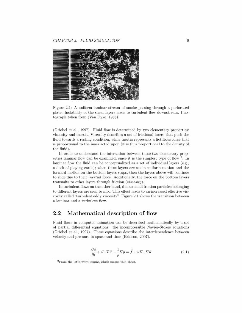
Figure 2.1: A uniform laminar stream of smoke passing through a perforatedplate. Instability of the shear layers leads to turbulent flow downstream. Pho-tograph taken from (Van Dyke, 1988).
(Griebel et al., 1997). Fluid flow is determined by two elementary properties:viscosity and inertia. Viscosity describes a set of frictional forces that push thefluid towards a resting condition, while inertia represents a fictitious force thatis proportional to the mass acted upon (it is thus proportional to the density ofthe fluid).
In order to understand the interaction between these two elementary prop-erties laminar flow can be examined, since it is the simplest type of flow 2. Inlaminar flow the fluid can be conceptualized as a set of individual layers (e.g.,a deck of playing cards); when these layers are set in uniform motion and theforward motion on the bottom layers stops, then the layers above will continueto slide due to their inertial force. Additionally, the force on the bottom layerstransmits to other layers through friction (viscosity).
In turbulent flows on the other hand, due to small friction particles belongingto different layers are seen to mix. This effect leads to an increased effective vis-cosity called “turbulent eddy viscosity”. Figure 2.1 shows the transition betweena laminar and a turbulent flow.
2.2 Mathematical description of flow
Fluid flows in computer animation can be described mathematically by a setof partial differential equations: the incompressible Navier-Stokes equations(Griebel et al., 1997). These equations describe the interdependence betweenvelocity and pressure in space and time (Bridson, 2007).
∂u
∂t+ u ·∇u+
1
ρ∇p = f + ν∇ ·∇u (2.1)
2From the latin word lamina which means thin sheet.

CHAPTER 2. FLUID SIMULATION 10
∇ · u = 0 (2.2)
Equation 2.1 is the momentum equation. It actually represents Newton’ssecond law, according to which a body of mass subject to a net force undergoesacceleration (F = ma). In simple terms, this equation describes the accelera-tion of the fluid due to forces acting upon it. The momentum equation standsactually for 3 equations in a wrapped up form, because the fluid’s velocity u
is a vector quantity. With some minor rearrangements, equation 2.1 can berewritten as follows:
∂u
∂t= −u ·∇u− 1
ρ∇p+ ν∇ ·∇u+ fx
∂v
∂t= −u ·∇v − 1
ρ∇p+ ν∇ ·∇v + fy
∂w
∂t= −u ·∇w − 1
ρ∇p+ ν∇ ·∇w + fz
Equation 2.2 is the continuity equation. This equation enforces the pre-viously mentioned incompressibility condition. Thus, the momentum and con-tinuity equations describe the motion of an incompressible and homogeneousfluid.
The incompressible Navier-Stokes equations at first sight may appear com-plicated. However, when the role of all individual terms in the formulas becomesclear then the actual meaning of these equations is fully revealed and it can beeasily comprehended. In the following sub-section the equation terms will bedissected into their elementary components.
2.2.1 Terms in the Navier-Stokes equationsThe most significant quantity which characterizes the state of the fluid at anyspecific time is its velocity u (Harris, 2004). The velocity of the fluid is rep-resented as a vector field u : R3 → R3. A vector field is a map that assignsa vector-valued function u(x) for every position x = (x, y, z), in a subset of aCartesian space. A vector field can be visually represented by assign each pointin the field an arrow pointing to a vector direction (e.g., see figure 2.2).
The symbol p represents the pressure of the fluid and signifies the force perunit area that the fluid exercises on its surroundings (and itself) (Bridson, 2008).Pressure builds up in the fluid when force is applied, as fluid molecules in thevicinity of the force push on those that lie farther away (Harris, 2004). The

CHAPTER 2. FLUID SIMULATION 11
Figure 2.2: A vector field plot. Figure modified from (Weisstein, 2011).
Figure 2.3: A visual representation of a scalar field. Figure taken from (Biały,2010).
pressure of the fluid is a scalar field; i.e., a map p : R3 → R that assigns eachpoint x in the Cartesian space a scalar-valued function p (x). A scalar field canbe visually represented by mapping the intensity of the field to a colour value(e.g., see figure 2.3).
The greek letter ρ in equation 2.1 represents the constant density of the fluid.For water, ρ is approximately 1000 kg/m3, and for air it is about 1.3 kg/m3
(Bridson, 2008). The greek letter ν in the momentum equation represents thefluid’s kinematic viscosity (a viscous acceleration). Finally, the vector quantityf represents any external forces that act upon the fluid.

CHAPTER 2. FLUID SIMULATION 12
2.2.1.1 Differential operators
The Nabla (or del) operator ∇ in equations 2.1 and 2.2 has three differentapplications: the gradient, the divergence and the Laplacian operators (Harris,2004).
The gradient of a scalar field is a vector of partial derivatives of the scalarfield (Bridson, 2008) (see equation 2.3). The gradient points in the directionof steepest descent, so the negative pressure gradient points away from high-pressure regions, towards low-pressure regions. Thus, the pressure gradientrepresents the imbalance in pressure or how high pressure regions push on lower-pressure regions.
∇p =
∂p
∂x,∂p
∂y,∂p
∂z
(2.3)
The divergence operator is the sum of partial derivatives of a vector field(it can only be applied to vector fields) and its output is a scalar quantity (seeequation 2.4). Divergence’s physical significance is the rate at which “density”exits a given region of space. Thus, in the absence of creation or destruction ofmatter, the density within a region of space can change only by flowing into orout of that region.
∇ · u =∂u
∂x+
∂v
∂y+
∂w
∂z(2.4)
The Laplacian is the divergence of the gradient. It measures how far lies aquantity from the average around it. As a result, the Laplacian of the velocityfield once integrated over the fluid volume provides a viscous force. In vectorfields the Laplacian is applied on every component separately (see equations 2.5to 2.7).
∇ ·∇u = ∇2u =
∂2u
∂x2+
∂2u
∂y2+
∂2u
∂z2(2.5)
∇ ·∇v = ∇2v =
∂2v
∂x2+
∂2v
∂y2+
∂2v
∂z2(2.6)
∇ ·∇w = ∇2w =
∂2w
∂x2+
∂2w
∂y2+
∂2w
∂z2(2.7)
2.2.2 The Euler equationsIn the turbulent flow of smoke, viscosity does not play a significant role, that iswhy it is possible to drop it completely. The incompressible Navier-Stokes equa-tions without the viscosity term are called the incompressible Euler equationsand they describe incompressible, inviscid fluids (Bridson, 2008) (see equations2.8 and 2.9).

CHAPTER 2. FLUID SIMULATION 13
∂u
∂t= −u ·∇u− 1
ρ∇p+ f (2.8)
∇ · u = 0 (2.9)
From now on and until the conclusion of this thesis the Euler equations willbe assumed as the employed mathematical model of fluid flow.
2.3 Solving the Euler equations
The Euler equations cannot be solved analytically for every physical configura-tion (Harris, 2004). However, numerical integration techniques can be used tosolve these equations incrementally, by discretizing the fluid domain.
There are two distinct approaches to discretize a physics problem in orderto numerically simulate it: the Lagrangian and the Eulerian approach (Wickeet al., 2007). Lagrangian methods discretize the material, and thus the simu-lation elements move with it. In fluid simulation particle based discretizationsare used, so that each particle has a position x and a velocity u. Each particleof the discretization represents a part of the fluid, so mass loss due to numer-ical error is not an issue. Moreover, moving boundaries and free surfaces areeasy to control, since the discretization moves along with the fluid. However,Lagrangian methods are not accurate in dealing with spatial derivatives on anunstructured particle cloud (Bridson, 2008). A popular Lagrangian method incomputer graphics is the Smooth Particle Hydrodynamics method.
Eulerian methods discretize the space in which the fluid moves and thus thefluid moves through the simulation elements, which are fixed in space. Thesimulation domain is divided into a set of volume elements called voxels. Thediscretization of space does not depend on the fluid and for this reason largedeformations such as those occurring in fluid motion can be managed efficiently.Eulerian methods are more robust in numerically approximating the spatialderivatives of the Euler equations. However, since the discretization of thesimulation domain does not change with the fluid’s shape, interface trackingand moving boundaries can be troublesome. Also, mass loss is possible to occur,due to numerical dissipation and as a result it may lead to an incorrect viscousforce. Figure 2.4 shows a comparison between the Eulerian and the Lagrangianmethods.
Hybrid methods that combine the two approaches also exist. In such meth-ods, particles can be advected through the velocity field and measurements canbe made on each particle. For example, smoke concentration can be measuredfor each particle in the simulation.
In this thesis the Eulerian approach has been selected for the discretizationof the fluid domain, due to the numerical accuracy that it offers.

CHAPTER 2. FLUID SIMULATION 14
Figure 2.4: A sphere of material discretized using Eulerian and Lagrangianmethods. Figure modified from (Wicke et al., 2007).
Figure 2.5: A cell-centered grid. Figure taken from (Stam, 1999).
2.3.1 Discretizing the fluidIn the Euler discretization, the vector and scalar-valued functions must bemapped onto a parameterized space, usually a Cartesian grid (Stam, 1999).The simplest structure that can be employed is a collocated (cell-centered) grid.In such a discretization, both vector and scalar fields are sampled at the centerof each cell (see figure 2.5).
Using this method all the differential operations can be approximated usingfinite differences. The central differences for each one of the differential opera-tors is described bellow3:
Gradient:
(∇p)i,,j,k =pi+1,j,k − pi−1,j,k
2δx,pi,j+1,k − pi,j−1,k
2δy,pi,j,k+1 − pi,j,k−1
2δz
Divergence:
(∇ · u)i,j,k =ui+1,j,k − ui−1,j,k
2δx+
vi,j+1,k − vi,j−1,k
2δy+
wi,j,k+1 − wi,j,k−1
2δz
3The subscripts i,j,k represent a cell’s position in the grid.

CHAPTER 2. FLUID SIMULATION 15
Laplacian:
∇2
ui,j,k
=ui+1,j,k − 2ui,j,k + ui−1,j,k
(δx)2+ui,j+1,k − 2ui,j,k + ui,j−1,k
(δy)2+ui,j,k+1 − 2ui,j,k + ui,j,k−1
(δz)2
∇2
vi,j,k
=vi+1,j,k − 2vi,j,k + vi−1,j,k
(δx)2+vi,j+1,k − 2vi,j,k + vi,j−1,k
(δy)2+vi,j,k+1 − 2vi,j,k + vi,j,k−1
(δz)2
∇2
wi,j,k
=wi+1,j,k − 2wi,j,k + wi−1,j,k
(δx)2+wi,j+1,k − 2wi,j,k + wi,j−1,k
(δy)2+wi,j,k+1 − 2wi,j,k + wi,j,k−1
(δz)2
2.3.2 Numerical simulationIn the field of computational fluid dynamics there are many methods to dis-cretize the Euler equations. In computer animation the method of splitting isthe most commonly used (Bridson 2008), (Crane et. al. 2007), (Harris, 2004).In this method each equation is split up into its component parts and each partis solved separately, one at a time (Bridson 2008). Thus, the simulation is di-vided in steps (or modules) and the output of the first step becomes the input ofthe second and so forth. It should be noted that the order of the steps is crucialfor the correct functioning of the simulation. The basic simulation pipeline isdescribed bellow:
Advection step:
∂u
∂t+ u ·∇u = 0
External forces step:
∂u
∂t= f
Pressure step:
∂u
∂t+
1
ρ∇p = 0 : ∇ · u = 0
However, it is still not apparent how these modules can be solved. Thefollowing subsection will describe a decomposition of the equations that willlead to a form that is compliant to a numerical solution.
2.3.3 Helmholtz-Hodge decomposition theoremAny vector can be represented as a sum of basis vector components (Harris,2004). For example, a vector u = (u, v, w) can be represented as u = ui+vj+wk,

CHAPTER 2. FLUID SIMULATION 16
Figure 2.6: The velocity field can become divergent-free when the pressuregradient is subtracted. Figure taken from (Stam, 2003).
where i, j and k are unit basis vectors that are aligned on the axis of a Cartesianspace. In the same way a vector field can be represented as a sum of vectorfields. In a region of space D with a differentiable boundary ∂D, and normaldirection n, the Helmholtz-Hodge theorem states that a vector field w on D canbe uniquely represented as:
w = u+∇p (2.10)
Where u is a divergence-free vector field, parallel to ∂D (u · n = 0 on ∂D).Thus, the theorem states that any vector field is the sum of a mass conserving
(divergent-free) field and the gradient of a scalar field. This result allows thedefinition of an operator P which projects the divergent velocity field w onto itsdivergence free part (u = P w) (Stam, 1999). The operator is defined implicitlyby applying the divergence operator on both sides of equation 2.10.
∇ · w = ∇2p
A solution to this equation, which is often called the Poisson-pressure equa-tion, can be used to compute the divergent free velocity field by subtracting thepressure gradient from the divergent velocity field (see figure 2.6):
u = P w = w −∇p
Using the projection operator P , the Euler equations can be rewritten asfollows4:
∂u
∂t= P
− (u ·∇) u+ ν∇2
u+ f
(2.11)
The solution of equation 2.11, over a single time step, can be defined as anoperator S(u) that takes the current velocity field u as its parameter (Harris,2004). S(u) is defined as the composition of three operators: A(u) for the
4Pu = u andP∇p = 0

CHAPTER 2. FLUID SIMULATION 17
Figure 2.7: Each step of the simulation produces a vector field w. At the laststep, field w2 is projected to a divergent-free space using the pressure projectionmethod. Figure modified from (Stam, 1999).
advection step, F for the external force application step, and P for the pressureprojection step (the operators are applied from right to left):
S (u) = P F A (u) (2.12)
The output of every operator is the new state of the velocity field. When thevelocity field reaches step 2, it will most probably be divergent. The pressureprojection operator projects the divergent velocity field to its divergent free part(figure 2.7 provides a visualization of this procedure, where every velocity fieldw corresponds to a step of the simulation).
2.3.4 Solving the Poisson pressure equationThe Poisson equation on a 3-dimensional domain Ω with a differentiable bound-ary ∂Ω follows the form (Noury et al., 2011):
∇2p = −f on Ω ⊂ R3 (2.13)
Where p signifies the solution of the Poisson equation and f is known. Inmost cases, equation 2.13 has no close-form solution for any given right-handside f and domain Ω. For this reason, a discretization scheme can be used andan approximation of the solution p can be sought in a finite-dimensional space.A very popular discretization method is the finite-volume method, where theaverage of p is approximated over a set of mesh cells that cover Ω. This meshis comprised by a set T of non-overlapping cells Ci:
Ω =
i∈TCi, Ci ∩ Cj = ∅, ∀i = j ∈ T

CHAPTER 2. FLUID SIMULATION 18
Using this discretization in 3 dimensions the Poisson equation in cell Ci,j,k
can be written as5:
6pi,j,k − pi−1,j,k − pi+1,j,k − pi,j−1,k − pi,j+1,k − pi,j,k−1 − pi,j,k+1 = −h2fi,j,k
(2.14)Or, in matrix form:
Ap = f (2.15)
Where A ∈ R3x3 represents a sparse matrix, p ∈ R3 represents the vectorthat contains the cell averages and f represents the right-hand side of equation2.14.
2.3.4.1 Iterative methods
The sparse matrix A displays two properties that make it invertible with aunique solution: it is symmetric and positive definite:
p = A−1
f
For small grid dimensions, this matrix can be inverted using a direct method(e.g., Gaussian elimination), however, such methods have many drawbacks: theyhave a O
N3
complexity, and require a lot of memory for storing the inverse
matrix (which is usually full) (Noury et al., 2011). For this reason iterativemethods can be used instead. In such methods an approximation of the Poissonsolution can be found using preconditioned iterations:
vα+1 =I − P
−1Avα + P
−1f (2.16)
Where, vα and vα+1 are the approximate solutions at iteration α and α+ 1respectively, and P represents a preconditioned in the linear system Ap = f .
The various available iterative solvers use different preconditioners. How-ever, in most cases, these preconditioners are constructed by decomposing thesparse matrix A into three components: L : the lower-triangular part of the ma-trix, D : the matrix diagonal, and U : the upper-triangular part of the matrix(see figure 2.8).
2.3.5 Boundary conditionsIn the Eulerian discretization scheme that has been used, the fluid is movinginside a 3D cube. However, so far its behavior on the boundaries has not beendefined. The simplest boundary condition for the velocity field is the no-stickcondition 6 (Bridson, 2008). For a static obstacle the condition specifies thatthe normal component of velocity must be zero at the boundary:
5Where h is the size of the uniform grid cells.6It applies to inviscid fluids.

CHAPTER 2. FLUID SIMULATION 19
Figure 2.8: Decomposition of the sparse matrix A. L: the low-triangular part,D, the diagonal, and U: the upper-triangular part. Figure modified from (Nouryet al., 2011).
u · n = 0
For, dynamic obstacles, however, the no-stick condition specifies that thenormal component of the fluid velocity must be equal to the normal componentof the obstacle velocity:
u · n = uobst · n
Using this condition the fluid is free to slip along the tangential direction ofthe obstacle.
A common boundary condition for the pressure field is the pure Neumanncondition where: ∂p
∂n = 0, for x ∈ ∂Ω (Harris, 2004). This means, that the rateof change of pressure along its normal component, must equal to zero at theboundary.
2.4 Solving for additional scalar fields
The main application of a fluid solver in computer animation is to use thevelocity field to move objects in a realistic fashion (Stam, 1999). In smokesimulation it is required to move smoke particles according to the velocity field.However, it is very computationally expensive to keep track of every particle.For this reason, the smoke particles can be replaced by a continuous densityfunction. This function stores the concentration of smoke particles in every cellof the grid.

CHAPTER 2. FLUID SIMULATION 20
Additional scalar fields can also be advected. A general formula that de-scribes the evolution of a quantity in the velocity field is described in equation2.17:
∂q
∂t= − (u ·∇) q + S (2.17)
In this equation q defines any quantity that is represented as a scalar fieldand S defines any sources that increase the amount of this quantity.

Chapter 3
Previous work
This chapter will describe previous works on fluid simulation in the field ofcomputer animation. The examination of these previous implementations hasbeen arranged in chronological order, as each new work has been influenced byprevious models.
3.1 Fluid solvers in computer animation
Before describing the research on GPU smoke solvers, it is crucial to examinethe structure of some well known fluid solver designed for computer animationapplications. For this reason, a short introduction will follow that will describeCPU models that have been implemented.
3.1.1 Foster and Metaxas (1996)Foster and Metaxas (Foster and Metaxas, 1996) developed one of the first meth-ods in computer animation that numerically solves the incompressible Navier-Stokes equations1. They used an explicit finite difference approximation of theequations that could be solved using an explicit Eulerian scheme. However,their method was not stable for any arbitrary time-step and that is why theyimposed the following constraint on the velocity field:
1 > max[uδt
δx, v
δt
δy, w
δt
δz]
3.1.2 Stam (1999)Stam (Stam, 1999) was the first to introduce an unconditionally stable methodfor simulating fluids. He used implicit integration schemes in every simulation
1Previous methods used procedural turbulence techniques that produced a pseudo-fluidmovement (Stam, 1999).
21

CHAPTER 3. PREVIOUS WORK 22
Figure 3.1: The semi-Lagrangian advection method. Figure taken from (Harris,2004).
step2 and hence large time-steps could be used, without compromising the sta-bility of the solver. The most important feature of his proposed solver was theadvection scheme; the so-called semi-Lagrangian advection, where the methodof characteristics is used to solve the partial differential equations. In simpleterms, the semi-Lagrangian advection method updates the velocity (or, indeed,any other scalar field) at a grid point xi,j,k by tracing back in time a source valuefrom the grid. To intuitively understand this, the advection can be thought ofas a Lagrangian process where particles move through the velocity field. At anytime t a particle can be moved from position xi,j,k, using the negative velocityui,j,k (t) (the velocity at grid position xi,j,k ). Using the negative velocity, willmove the particle in its position one time-step ago. However, the particle willmost likely end up in a position in-between grid cells or even outside the grid.In order to find an approximate value from that position, trilinear interpolationcan be used on the closest neighboring cells. The resulting value will then beused as the updated value in position xi,j,k. Figure 3.1 describes this process.
Although this advection scheme is unconditionally stable, it introduces nu-merical dissipation to the simulation (Bridson, 2008). In order to overcome thisproblem, higher accuracy interpolation schemes can be used.
3.1.3 Fedkiw et al. (2001)Fedkiw et al. (Fedkiw et al., 2001) described a method for the visual simulationof smoke. Their solver has many similarities with Stam’s method; however,in order to simulate the movement of the smoke particles, they have added a
2With the only exception of the force application step, where explicit integration can besafely used.
CHAPTER 3. PREVIOUS WORK 23
temperature and a density field. Both these fields affect the evolution of thevelocity field: dense smoke has a tendency to fall downwards, because of gravity,while hot smoke tends to rise, due to buoyant forces. In order to accommodatethese interactions, they used a simple model, where a buoyant force proportionalto the smoke velocity and temperature is added to the velocity field:
fbuoy = −αρz + β(T − Tamb)z (3.1)
Where ρ represents density, T represents temperature, Tamb represents theambient temperature of the air, z is the buoyancy direction and α and β aretwo positive constants.
3.2 GPU implementations
In this section three GPU based smoke solvers will be described.
3.2.1 Harris (2004)Harris (Harris, 2004) described one of the first GPU methods for stable fluidsimulation on the GPU. His 2D solver follows the method proposed by Stam.For the representation of the simulation fields 2D textures are used and the sim-ulation kernels run on fragment programs. Every simulation step is preformedby rendering a 2D quad and executing the appropriate fragment program. Thefragment programs that are used by the solver are described below:
• Advect: this program performs the semi-Lagrangian advection step.
• Diffuse: this program is responsible for the viscous diffusion step. How-ever, as stated before, this step can be skipped in smoke simulation.
• Apply force: in this module, force is applied to the velocity field.
• Divergence: this program calculates the divergence of the velocity field.The divergence field is used in the Poisson solver, in order to perform thepressure projection step.
• Jacobi: this program uses the Jacobi iteration method to solve the Pois-son equations.
• Subtract gradient: this kernel calculates the pressure gradient usingfinite differences, and it subtracts it from the velocity field. This is thepart of the simulation where the incompressibility condition is enforced.
• Boundary: the simulation boundary values are stored in 4 line primi-tives. These primitives hold values for both the velocity and the pressureboundary conditions.

CHAPTER 3. PREVIOUS WORK 24
Figure 3.2: Voxelization of complex geometry. The collision and velocity texturemaps are displayed on the right. Figure taken from (Crane et al., 2007).
3.2.2 Crane et al. (2007)Crane et al. (Crane et al., 2007) expanded Harris’ method and introduced amore advanced solver that can be used in any rasterization-based renderingparadigm. One of the new features that they introduced to their model was thehandling of dynamic obstacles. They use a voxelization scheme, where everygeometry can be mapped to a voxel map. They store two separate texturemaps for this operations: one for the collision data (where a voxel is markedeither as occupied or as free) and one for the velocity data (where the obstaclevelocity data are stored on the object’s boundary) (see figure 3.2). This methodfacilitates the enforcement of the no-stick boundary conditions and thus allowsthe fluid to flow around a moving obstacle.
3.2.3 Rideout (2011)Rideout (Rideout, 2011) created a solver that is based on the two previousimplementations. It uses frame-buffer operations for the execution of the sim-ulation programs, and every field is represented as a 3D texture. The solveralso features an impulse application step where smoke density and temperatureare introduced to the simulation. The managing of both boundary and obstacleconditions is handled using voxel maps (similar to the approach of Crane et al.)so all the simulations collision and velocity data are stored in one texture. Thepipeline of this application is displayed in figure 3.3:

CHAPTER 3. PREVIOUS WORK 25
Figure 3.3: The application diagram of Rideout’s implementation. Figure takenfrom (Rideout, 2010).

Chapter 4
Implementation
In this chapter the implemented smoke simulation application is described.Firstly, the OpenCL standard will be discussed and subsequently the designand implementation of the application will be analyzed.
4.1 OpenCL overview
OpenCL is an open standard for programming in heterogeneous systems, that is,systems comprised of multiple parallel processing units (referred to as devicesin the OpenCL lingo) like multicore CPUs and GPUs (Noury et al., 2011),(Munshi et al., 2011). The OpenCL pipeline can be divided into two distinctparts. In the first part, a CPU based host runs OpenCL API commands thatcreate memory objects on the devices, manage the execution of parallel programsand control the interactions between host and devices (in the same way thatthe OpenGL/GLSL pipeline works) (Noury et al., 2011). In the second part,parallel programs (called compute kernels) written in the OpenCL C languageare executed on the devices (in the same way as shader programs).
4.1.1 Execution modelWhen the host issues a kernel execution command, the OpenCL runtime systemgenerates an integer index space (Munshi et al., 2011). This space can have anN-dimension range of values and thus it is referred to as the kernel NDRange.The compute kernel is executed once for each point in the NDRange. Eachthread of the executing kernel is called a work-item and is uniquely identifiedby its index space coordinates. These coordinates constitute the global ID ofthe work-item.
The NDRange is divided into groups of work-times; these thread rangesare called work-groups. Every work-group has an ID in the NDRange and everywork-item in the group has a local ID defining its local coordinates. This divisionscheme is described in figure 4.1.
26

CHAPTER 4. IMPLEMENTATION 27
Figure 4.1: A 2D NDrange displaying all the possible work-item coordinatecategorizations, G: global coordinates, W: work-group coordinates, L: local co-ordinates. Figure taken from (Munshi et al., 2011).
4.1.2 Memory modelOpenCL specifies two kinds of memory objects: buffer objects and image ob-jects. Buffers are contiguous blocks of memory indexed by 1D coordinates andcomposed of any available OpenCL data type (int, float, half, double, int2, int3,int4, float2, ...) (Noury et al., 2011). Any data structure can be mapped ontoa buffer and its data can be accessed through pointers (Munshi et al., 2011).
Images have many similarities with OpenGL textures: they both supportan automatic caching mechanism and their data are accessed through samplerobjects (Noury et al., 2011). Samplers can filter the image data using multilinearinterpolation, and, furthermore, they allow the configuration of out of boundaccess behavior.
In addition to the memory object types, the OpenCL memory model specifies5 regions, where data can be allocated (Munshi et al., 2011):
• Host memory: this region is exclusively visible by the host. It is usedfor interactions between the host and OpenCL objects.
• Global memory: this region gives access to reading and writing opera-tions to all the work-items in every work-group. Global memory connectsthe host and the employed devices by enqueuing reading and writing op-erations. It has a large scale capacity, but it also has high latency.
• Constant memory: it represents a region of global memory that staysconstant through a kernel execution (similar to a shader uniform). Datastored in constant memory can only be read by the compute kernels.
CHAPTER 4. IMPLEMENTATION 28
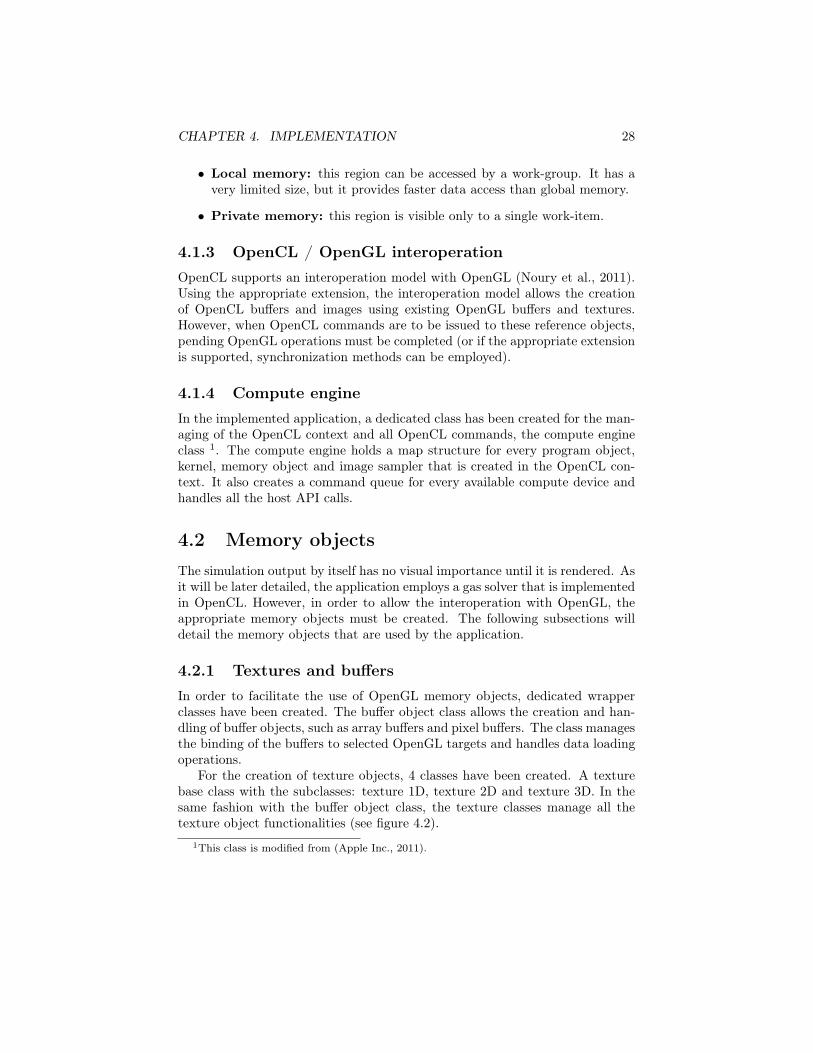
• Local memory: this region can be accessed by a work-group. It has avery limited size, but it provides faster data access than global memory.
• Private memory: this region is visible only to a single work-item.
4.1.3 OpenCL / OpenGL interoperationOpenCL supports an interoperation model with OpenGL (Noury et al., 2011).Using the appropriate extension, the interoperation model allows the creationof OpenCL buffers and images using existing OpenGL buffers and textures.However, when OpenCL commands are to be issued to these reference objects,pending OpenGL operations must be completed (or if the appropriate extensionis supported, synchronization methods can be employed).
4.1.4 Compute engineIn the implemented application, a dedicated class has been created for the man-aging of the OpenCL context and all OpenCL commands, the compute engineclass 1. The compute engine holds a map structure for every program object,kernel, memory object and image sampler that is created in the OpenCL con-text. It also creates a command queue for every available compute device andhandles all the host API calls.
4.2 Memory objects
The simulation output by itself has no visual importance until it is rendered. Asit will be later detailed, the application employs a gas solver that is implementedin OpenCL. However, in order to allow the interoperation with OpenGL, theappropriate memory objects must be created. The following subsections willdetail the memory objects that are used by the application.
4.2.1 Textures and buffersIn order to facilitate the use of OpenGL memory objects, dedicated wrapperclasses have been created. The buffer object class allows the creation and han-dling of buffer objects, such as array buffers and pixel buffers. The class managesthe binding of the buffers to selected OpenGL targets and handles data loadingoperations.
For the creation of texture objects, 4 classes have been created. A texturebase class with the subclasses: texture 1D, texture 2D and texture 3D. In thesame fashion with the buffer object class, the texture classes manage all thetexture object functionalities (see figure 4.2).
1This class is modified from (Apple Inc., 2011).

CHAPTER 4. IMPLEMENTATION 29
Figure 4.2: The application memory objects.
4.2.1.1 Texture image unit stack
When a texture object is created, it must be attached to a texture image unit.The number of the available image units depends on the GPU capabilities andthe OpenGL implementation. Although it is possible to attach two or moretextures on the same unit, when these textures are used in the same shaderonly one of them will be sampled (and it is undefined which one). In order tofacilitate the creation of textures in a rendering context,2 a utility class has beencreated: the texture image unit stack. It is a stack structure that stores all theavailable texture image units and returns the next available unit.
4.2.2 Ping-pong volumesTexture objects can be ideal candidates for the representation of the simulationfields. They internally support trilinear interpolation and allow configurableout of bounds behavior, features which are fundamental in the gas solver func-tionality. However, currently most OpenCL implementations do not supportin-kernel writing operation on 3D images. For this reason, a turnaround can beemployed in order to overcome this restriction. A referenced pixel buffer object(PBO) can be used as the writing target in the compute kernels: at the end ofeach solver cycle, the PBO data can be uploaded to a 3D texture by enqueuing acopy command. Although the copy command adds overhead to the application,it still remains a GPU located operation, so the simulation data never actuallyleave the GPU. In order to accommodate for these reading and writing opera-tions, a ping-pong volume class has been created. It is a volume object that usesa PBO for all writing operations and a 3D texture for all reading operations. Ituses a swap method for the uploading of the PBO data to the texture. In thisway, the benefits of 3D texture data access in OpenCL are preserved by addingan extra step to the data writing operation. In order to reference the OpenGLmemory objects of the volume, two references must be created in OpenCL: a3D image reference and a buffer reference.
2A context where multiple shaders share a common set of resources.

CHAPTER 4. IMPLEMENTATION 30
Algorithm 4.1 The advection kernel.
// check f o r ob s t a c l e s and boundaryIF ( c e l l [ i , j , k ] == SOLID) THEN
f i e l d [ i , j , k ] = 0 ;EXIT
// f i nd c e l l c oo rd ina t e s "back in time"[ i0 , j0 , k0 ] = [ i , j , k ] − dt ∗ V[ i , j , k ] ;
f i e l d [ i , j , k ] = d i s s i p a t i onFac t o r ∗ V[ i0 , j0 , k0 ] ;
Algorithm 4.2 The buoyancy application kernel.
IF (T[ i , j , k ] > ambientTemperature ) THEN
V[ i , j , k ] += (dt ∗ (T[ i , j , k ] − ambientTemperature )∗ buoyancyLi ft − D[ i , j , k ] ∗ gasWeight
) ∗ buoyancyDirect ion ;
4.3 The gas solver
This section will detail all the different modules of the implemented gas solver.
4.3.1 AdvectionThe advection kernel performs semi-Lagrangian advection on the velocity, tem-perature and density fields. In order to find the coordinates of the particle onetime-step back, forward Euler integration is used. Algorithm listing 4.1 displaysthe pseudocode of the kernel where cell[i,j,k] corresponds to a grid position atpoint (i,j,k), field[i,j,k] corresponds to any field value at the current position andV stands for the current velocity.
4.3.2 Buoyancy applicationThe buoyancy application kernel is responsible for the buoyant force that makesdense smoke sink and hot smoke rise. The buoyant force is applied to cells wherethe temperature is greater than the ambient temperature. Algorithm listing 4.2displays the pseudocode of the kernel, where T represents the temperature fieldand D represents the density field.

CHAPTER 4. IMPLEMENTATION 31
Algorithm 4.3 The impulse application kernel.
IF ( c e l [ i , j , k ] == INSIDE−SPLAT−REGION) THEN
D[ i , j , k ] = densityAmount ;T[ i , j , k ] = temperatureAmount ;
Figure 4.3: Iso-surface voxelization for a sphere surface. The obstacle objectcontains an instance of the simulation boundary.
4.3.3 Impulse applicationThe impulse application kernel acts as a source for temperature and smokedensity. The sources are added using a Gaussian splat; that is, cells that areinside the splat radius will be assigned a specified amount of temperature anddensity. Algorithm listing 4.3 displays the kernel pseudocode:
4.3.4 Adding obstaclesObstacles are added into the simulation, using implicit surfaces. In order tovoxelize the surfaces, an implicit surface is sampled on the simulation grid; if acell contains an iso-value that is less than zero, then this cell is marked as solid.In order to merge the boundary checks with the obstacle collision detection,every obstacle object contains an instance of the simulation boundary (see figure4.3). The gas solver also supports the use of dynamic obstacles; however, movingobstacles have not yet been implemented in the application and all obstacles areassumed to be stopped with zero velocity (the boundary is also considered anobstacle with zero velocity).
4.3.5 Pressure projectionIn the pressure projection step, the differentiation operators of the incompress-ible Euler equations are approximated using central differences. In order to
CHAPTER 4. IMPLEMENTATION 32
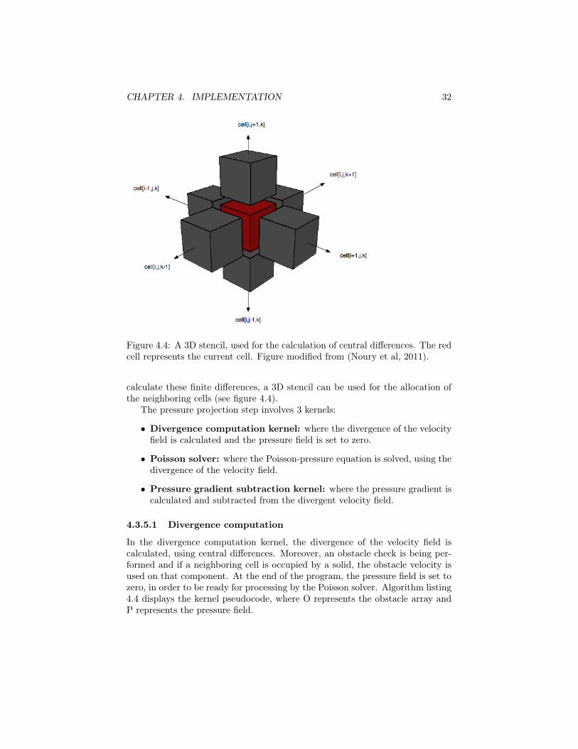
Figure 4.4: A 3D stencil, used for the calculation of central differences. The redcell represents the current cell. Figure modified from (Noury et al, 2011).
calculate these finite differences, a 3D stencil can be used for the allocation ofthe neighboring cells (see figure 4.4).
The pressure projection step involves 3 kernels:
• Divergence computation kernel: where the divergence of the velocityfield is calculated and the pressure field is set to zero.
• Poisson solver: where the Poisson-pressure equation is solved, using thedivergence of the velocity field.
• Pressure gradient subtraction kernel: where the pressure gradient iscalculated and subtracted from the divergent velocity field.
4.3.5.1 Divergence computation
In the divergence computation kernel, the divergence of the velocity field iscalculated, using central differences. Moreover, an obstacle check is being per-formed and if a neighboring cell is occupied by a solid, the obstacle velocity isused on that component. At the end of the program, the pressure field is set tozero, in order to be ready for processing by the Poisson solver. Algorithm listing4.4 displays the kernel pseudocode, where O represents the obstacle array andP represents the pressure field.

CHAPTER 4. IMPLEMENTATION 33
Algorithm 4.4 The divergence computation kernel.
// f i nd v e l o c i t y s t e n c i l (up , down , r i ght , l e f t , f r on t and back )Vu = V[ i , j +1,k ] ;Vd = V[ i , j −1,k ] ;Vr = V[ i +1, j , k ] ;Vl = V[ i −1, j , k ] ;Vf = V[ i , j , k+1] ;Vb = V[ i , j , k−1] ;
// f i nd ob s t a c l e s t e n c i lOu = O[ i , j +1,k ] ;Od = O[ i , j −1,k ] ;Or = O[ i +1, j , k ] ;Ol = O[ i −1, j , k ] ;Of = O[ i , j , k+1] ;Ob = O[ i , j , k−1] ;
// i f c e l l i s s o l i d use ob s t a c l e v e l o c i t yIF (Ou == SOLID) THEN vU = oU ; IF (Od == SOLID) THEN vD = oD; IF (Or == SOLID) THEN vR = oR ; IF (Ol == SOLID) THEN vL = oL ; IF (Of == SOLID) THEN vF = oF ; IF (Ob == SOLID) THEN vB = oB ;
// compute d ive rgence f i e l dd ive rgence [ i , j , k ] = (Vr . x − Vl . x + Vu. y − Vd. y + Vf . z − Vb. z ) / 2∗ c e l l S i z e ;P [ i , j , k ] = 0 ;

CHAPTER 4. IMPLEMENTATION 34
4.3.5.2 Pressure gradient subtraction
The pressure gradient subtraction kernel calculates the pressure gradient andsubtracts it from the velocity field. It also sets the boundary conditions by usingthe neighboring pressure on solid cells, and by enforcing the no-stick condition.Algorithm listing 4.5 displays the pseudocode of the kernel.
4.3.5.3 Poisson solver
A common iterative method for the solution of the Poisson-pressure equationis the Jacobi iteration method (Noury et al., 2011). This method can be par-allelized easily on a GPU implementation and has been used by Harris, Craneet al. and Rideout (Rideout, 2011), (Crane et al., 2007), (Harris, 2004). TheJacobi method uses the diagonal of the sparse matrix A (see equation 2.15) asits preconditioner Pj = D. Thus, equation 2.16 can be written as 3:
vα+1 =
I − 1
6A
vα +
1
6f (4.1)
Equation 4.1 can be easily translated into a compute kernel (see algorithmlisting 4.6).
4.3.6 Adding turbulenceThe solvers allows additional control over the simulation by adding proceduralnoise to the velocity field. The periodic noise function adds randomness tothe buoyancy direction and allows the configuration of a trigonometric drivingfunction (sine, cosine, and tangent functions). This method provides additionalcontrol over the fluid motion and enhances the smoke detail.
4.4 Real-time rendering
The most interesting output in the smoke simulation is its density field. In thissection, two volume rendering technique that produce a visual output of thesimulation data will be described.
4.4.1 The marching cubes algorithmThe marching cubes algorithm was originally developed for the visualizationof medical data (mainly data from MRI or CT scans) (Lorensen and Cline,1987). However, it can also be used for the visualization of any scalar field.The algorithm performs a polygonization operation on constant density data,which are represented in the form of a 3D array. The algorithm progresses inthe following steps:
3In a 3D Laplace matrix the diagonal is equal to 6, thus, D−1 = 16 I (Noury et al., 2011).

CHAPTER 4. IMPLEMENTATION 35
Algorithm 4.5 The pressure gradient subtraction kernel.
IF ( c e l l [ i , j , k ] == SOLID) THEN
V[ i , j , k ] = OBSTACLE VELOCITY;EXIT
// f i nd pr e s su r e s t e n c i lPu = P[ i , j +1,k ] ;Pd = P[ i , j −1,k ] ;Pr = P[ i +1, j , k ] ;Pl = P[ i −1, j , k ] ;Pf = P[ i , j , k+1] ;Pb = P[ i , j , k−1] ;
// f i nd ob s t a c l e s t e n c i lOu = O[ i , j +1,k ] ;Od = O[ i , j −1,k ] ;Or = O[ i +1, j , k ] ;Ol = O[ i −1, j , k ] ;Of = O[ i , j , k+1] ;Ob = O[ i , j , k−1] ;
// use cente r p r e s su r e f o r s o l i d c e l l sVobstac le = ( 0 , 0 , 0 ) ;Vmask = ( 1 , 1 , 1 ) ;
IF (Ou == SOLID) THEN Pu = P[ i , j , k ] ; Vobstac le . y = Ou. z ; Vmask . y = 0 ; IF (Od == SOLID) THEN Pd = P[ i , j , k ] ; Vobstac le . y = Od. z ; Vmask . y = 0 ; IF (Or == SOLID) THEN Pr = P[ i , j , k ] ; Vobstac le . x = Or . y ; Vmask . x = 0 ; IF (Ol == SOLID) THEN Pl = P[ i , j , k ] ; Vobstac le . x = Ol . y ; Vmask . x = 0 ; IF (Of == SOLID) THEN Pf = P[ i , j , k ] ; Vobstac le . z = Of . x ; Vmask . z = 0 ; IF (Ob == SOLID) THEN Pb = P[ i , j , k ] ; Vobstac le . z = Ob. x ; Vmask . z = 0 ;
// en f o r c e the no−s t i c k boundary cond i t i onVold = V[ i , j , k ] ;g rad i ent = (Pr − Pl , Pu − Pd , Pf − Pb) ∗ g rad i en tSca l e ;Vnew = Vold − grad i ent ;V[ i , j , k ] = (Vmask ∗ Vnew) + Vobstac le ;

CHAPTER 4. IMPLEMENTATION 36
Algorithm 4.6 The Poisson solver kernel.
// f i nd pr e s su r e s t e n c i lPu = P[ i , j +1,k ] ;Pd = P[ i , j −1,k ] ;Pr = P[ i +1, j , k ] ;Pl = P[ i −1, j , k ] ;Pf = P[ i , j , k+1] ;Pb = P[ i , j , k−1] ;
P [ i , j , k ] = ( Pl + Pr + Pd + Pu + Pf + Pb − (h∗h) ∗ f [ i , j , k ] ) / 6 ;
1. The scalar field is being examined in respect to a user-defined thresholdvalue. When implicit surface modeling is considered, this value should be0, so that it defines the points that lie on the surface.
2. The finite volume of the discretization is comprised of cubes that form agrid structure. For every cube, a set of vertices that are intersected bythe surface are calculated. These vertices are calculated on the edges ofeach cube. The exact position of a vertex is configured through a linearinterpolation scheme which follows the sampled values. This calculationis performed with the use of an edge look-up table.
3. For the actual triangulation of the vertices, a triangulation look-up tableis used (Bourke, 1994). This table defines the sequence of the verticesin a manner that can be rendered by a graphics API (usually counterclockwise).
4. Finally, the normals for each vertex are computed by calculating the sur-face gradient at each cube corner and by linearly interpolating betweenthese gradient values.
Due to the fact that a cube has 8 vertices, there are totally 28 = 256 waysby which a surface can intersect a cube. However, because of two symmetricalproperties of the topology of the cube these cases can be reduced to 14 uniquepatterns. These patterns are depicted in figure 4.5:
The class of each cube can be represented using a single byte. The byte isinitialized with 0 and for each vertex that satisfies the threshold condition (aniso value in the case of implicit surfaces) we assign a 1. The numbering of thevertices and the edges of each cube are depicted in figure 4.6.
The edges that are intersected by the surface can be determined by calcu-lating the class (index) of the cube. In order to find the exact position of everytriangle vertex, a linear interpolation can be performed with two weights: eachweight corresponds to the sampled value at the two vertices that belong to anintersected edge. The intersected edges are determined by an edge, look-uptable. The edge table returns a 12 bit number for every cube class (256 cells),

CHAPTER 4. IMPLEMENTATION 37
Figure 4.5: The marching cubes cases. Figure taken from (Favreau, 2006).
Figure 4.6: Cube edge and vertex indices. Figure taken from (Lorensen andCline, 1987).
CHAPTER 4. IMPLEMENTATION 38
each bit corresponds to an edge; its value is zero, if the edge is not intersectedby the iso-surface, and one, if the edge is intersected by the iso-surface (Bourke,1994).
The triangulation table holds the sequence of vertex indices. It is a 2D tablewhich has 256 rows (one for each cube class) and 16 rows, since the maximumnumber of produced triangles is 5. The last row marks the end of a trianglesequence (for the classes that produce 5 triangles).
4.4.1.1 Surface shading
The last part of the marching cubes algorithm calculates a normal for eachvertex. The normal vector is required if any BRDF (Bidirectional ReflectanceDistribution Function) model is to be used. One of the most common methodsto compute the iso-surface normals is to use the gradient of the field function,which is actually the normal of the surface (Bloomenthal, 2001), (Nielson et al.,2002) (see equation 4.2).
N (x, y, z) = ∇F (x, y, z) =
∂F
∂x(x, y, z) ,
∂F
∂y(x, y, z) ,
∂F
∂z(x, y, z)
(4.2)
Consequently, a numerical differentiation method can be employed for theapproximation of the spatial derivatives. This calculation must be performedfor every cube’s vertex and the normal for every triangle vertex can be foundthrough interpolation along the cube edges.
4.4.1.2 GPU marching cubes
Programmable geometry shaders are a relatively new addition to the graphicspipeline. They take place after vertex processing and before viewport clipping(Wright et al., 2010). Unlike vertex and fragment (or pixel) shaders, where eachprocessing cycle accesses only one unit (vertex or fragment), geometry shadershave access to whole primitives (e.g, lines, triangles). Geometry shaders canperform a certain amount of tessellation (their capabilities are not immense,however) by producing new geometry and they can also discard geometry.
One of the first implementations of the marching cubes algorithm was pre-sented in SIGGRAPH 2006 by Tariq (Tariq, 2006) (for DirectX10). A similarapproach has been also demonstrated by Crassin (Crassin, 2007) (for openGL).
The VolumeMesher class encapsulates all the functionality that is requiredfor the rendering of a scalar field, using the GPU marching cubes algorithm 4.The look-up tables and the density field are stored in textures and only the gridcell centers are uploaded to the vertex processor. Apart from the configuration
4It also supports the dividing cubes algorithm, which renders the whole voxel cubes thatare occupied by the field.
CHAPTER 4. IMPLEMENTATION 39
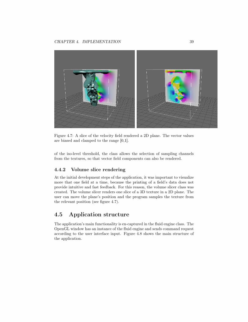
Figure 4.7: A slice of the velocity field rendered a 2D plane. The vector valuesare biased and clamped to the range [0,1].
of the iso-level threshold, the class allows the selection of sampling channelsfrom the textures, so that vector field components can also be rendered.
4.4.2 Volume slice renderingAt the initial development steps of the application, it was important to visualizemore that one field at a time, because the printing of a field’s data does notprovide intuitive and fast feedback. For this reason, the volume slicer class wascreated. The volume slicer renders one slice of a 3D texture in a 2D plane. Theuser can move the plane’s position and the program samples the texture fromthe relevant position (see figure 4.7).
4.5 Application structure
The application’s main functionality is en-captured in the fluid engine class. TheOpenGL window has an instance of the fluid engine and sends command requestaccording to the user interface input. Figure 4.8 shows the main structure ofthe application.
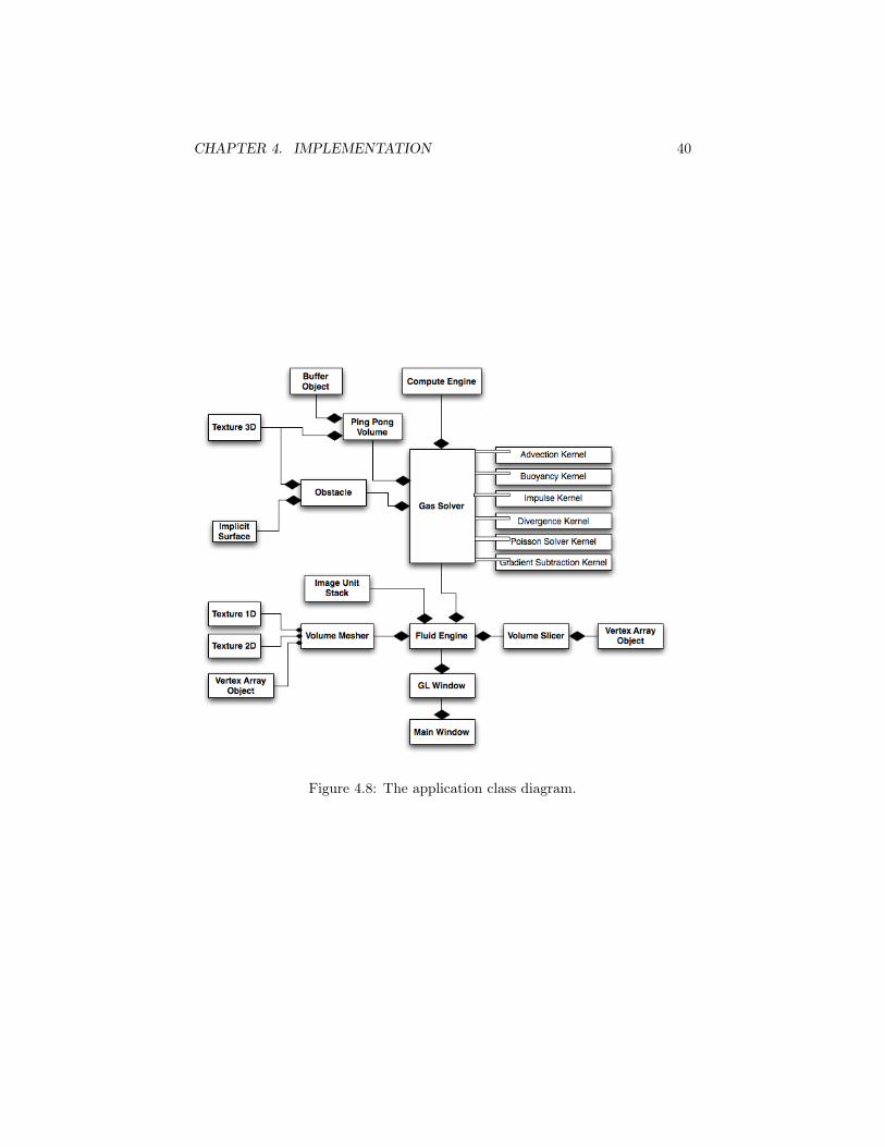
CHAPTER 4. IMPLEMENTATION 40
Figure 4.8: The application class diagram.

Chapter 5
Conclusion
In this last chapter the outcomes of the proposed application are discussed,pinpointing issues that were encountered.
5.1 Results
The solver can produce interactive and realistic smoke flow at a resolution of32x32x32. Figure 5.1 demonstrates an example simulation at this resolution:
Implicit surface obstacles can be used in order to sculp the smoke accordingto their shape. Figures 5.2 and 5.3 show interactions of smoke with staticobstacles.
Interesting results can be attained when noise is introduced to the velocityfield. Figure 5.4 exhibits a turbulent buoyant force that is driven by a trigono-metric function (pure noise, sine, cosine and tangent functions respectively).
A grid resolution of 64x64x64 produces especially detailed results. Figure5.5 shows two example smoke simulations at that resolution.
5.2 Efficiency
The application was developed on a Macbook pro using an NVIDIA GeForce320M, with 256 MB of virtual memory. Although the speed of the applicationwas not extraordinary high, it could still provide real time interaction with thesystem. Table 5.1 demonstrates the average frames per second for 4 differentgrid resolutions.
5.3 Known issues
One problem that has not been resolved in the final implementation is relatedwith the advection step. The advected fluids display a slight tendency to followthe vector (-1,-1,-1). A solution to this problem could be a more accurate
41

CHAPTER 5. CONCLUSION 42
Figure 5.1: A 32x32x32 grid example simulation.
Figure 5.2: Smoke interacting with a sphere.
Grid resolution FPS8x8x8 38
16x16x16 2032x32x32 764x64x64 3
Table 5.1: The application speed on different grid resolutions.

CHAPTER 5. CONCLUSION 43
Figure 5.3: Smoke interacting with a torus.
Figure 5.4: Interesting fluid motion can be achieved using the periodic noisefunction. The figures show an example smoke simulation using the standardnoise function, the sine driven function, the cosine driven function and thetangent driven function.

CHAPTER 5. CONCLUSION 44
Figure 5.5: Two example simulations at a resolution of 64x64x64. The rightpicture was produced with the use of the periodic noise method.
advection scheme, such as the MacCormack method. However, this deviation isnot always visible and it dissolves if the external forces are strong enough.
Another issue that is apparent in the application is the polygonal represen-tation of the fluid. Even though the mesh is accurate and it is rendered fast, theoutcome does not look like a gaseous fluid; it rather appears more like a plasticsolid (like clay). However, the focus of this thesis has been placed more on thesimulation process than on photorealistic rendering.
5.4 Future work
Future work might concentrate on the implementation of a GPU ray-caster,so that the generated smoke may look more like a gaseous fluid. Additionally,it would be interesting, if a faster Poisson solver could be implemented (forexample, a multi-grid solver).

Chapter 6
Bibliography
1. Apple Inc., 2006. OpenCL procedural grass and terrain example. Cuper-tino: Apple Inc.. Available from: http://developer.apple.com [Accessed25 May 2011].
2. Biały, S., 2010. Scalar field [figure]. http://en.wikipedia.org. Availablefrom: http://upload.wikimedia.org/wikipedia/en/f/fe/Scalarfield.jpg [Ac-cessed 30 May 2011].
3. Bloomenthal, J., 2001. Implicit surfaces. In: Henderson, H., ed., Encyclo-pedia of Computer Science and Technology. New York, NY, USA: MarcelDekker, Inc..
4. Bourke, P., 1994. Polygonising a scalar field. Cupertino: http://paulbourke.netAvailable from: http://paulbourke.net/geometry/polygonise [Accessed 1April 2011].
5. Bridson, R., 2008. Fluid simulation for computer graphics. Natick, MA,USA: A K Peters.
6. Bridson, R. and Muller-Fischer, M., 2007. Fluid simulation: SIGGRAPH2007 course notes. ACM SIGGRAPH.
7. Crane, K., Llamas, I., and Tariq, S., 2007. Real-time simulation andrendering of 3D fluids. In Nguyen, H., editor, GPU Gems 3. Indiana, IN,USA: Addison-Wesley Professional.
8. Crassin, C., 2007. OpenGL geometry shader marching cubes. http://paulbourke.netAvailable from: http://paulbourke.net/geometry/polygonise [Accessed 1April 2011].
9. Favreau, J., M., 2006. Marching cubes cases [figure]. http://commons.wikimedia.org.Available from: http://en.wikipedia.org/wiki/File:MarchingCubes.svg [Ac-cessed 3 April 2011].
45
CHAPTER 6. BIBLIOGRAPHY 46
10. Fedkiw, R., Jos, S., and Henrik, J., 2001. Visual simulation of smoke. InSIGGRAPH ’01: Proceedings of the 28th annual conference on computergraphics and interactive techniques, pages 15–22. ACM.
11. Foster, N., and Metaxas, D., 1996. Realistic animation of liquids. Graph-ical models and image processing, 58(5).
12. Griebel, M., Dornsheifer, T., and Neunhoeffer, T., 1997. Numerical Sim-ulation in Fluid Dynamics: A Practical Introduction. (Monographs onMathematical Modeling and Computation). SIAM: Society for Industrialand Applied Mathematics.
13. Harris, M. J., 2004. Fast fluid dynamics simulation on the GPU. In R.Fernando, ed., GPU Gems: Programming Techniques, Tips and Tricks forReal- Time Graphics, pages 637–665. Indiana, IN, USA: Addison-WesleyProfessional.
14. Lorensen W. E., and Cline, H. E., 1987. Marching cubes: A high resolution3D surface construction algorithm. ACM Siggraph Computer Graphics,21(4) : 163– 169.
15. Munshi, A., Gaster, B., Mattson, T., Fung, J., and Ginsburg, D., 2011.OpenCL programming guide. Addison-Wesley Professional.
16. Nielson, G. M., Huang, A., and Sylvester, S., 2002. Approximating nor-mals for marching cubes applied to locally supported isosurfaces. VIS2002. IEEE, pages 459–466.
17. Noury, S., Boivin, S., and Le Maitre, O, 2011. A fast Poisson solver forOpenCL using Multigrid methods. In Engel, W., ed., GPU Pro 2. A KPeters.
18. Rideout, P., 2010. Simple fluid simulation. http://prideout.net/blog/.Available from: http://prideout.net/blog/?p=58 [Accessed 28 May 2011].
19. Rideout, P., 2011. 3D Eulerian grid. http://prideout.net/blog/. Availablefrom: http://prideout.net/blog/?p=66 [Accessed 28 May 2011].
20. Stam, J., 1999. Stable fluids. In Proceedings of the 26th annual conferenceon Computer graphics and interactive techniques, SIGGRAPH ’99, pages121– 128, New York, NY, USA: ACM, Press/Addison–Wesley PublishingCo.
21. Stam, J., 2003. Real-time fluid dynamics for games. In Proceedings ofthe Game Developer Conference, pages 1–17.
22. Tariq, T., 2006. DirectX10 Effects. In SIGGRAPH 2006, page 626. Word-ware Publishing.
23. Van Dyke, M., 1988. Album of Fluid Motion. Parabolic Press, Inc., 4thedition.
CHAPTER 6. BIBLIOGRAPHY 47
24. Weisstein, E. W., 2011. Vector field plot. MathWorld - A Wolfram web re-source. Available from: http://140.177.205.23/VectorField.html [Accessed1 June 2011].
25. Wicke, M., Keiser, R., and Gross, M., 2007. Fluid simulation. In Gross,M. and Pfister, H., eds., Point-based graphics. Morgan Kaufmann.
26. Wright, R. S. , Haemel, N. , Sellers, G., and Lipchak, B., 2010. OpenGLSuperBible: Comprehensive Tutorial and Reference. Addison-Wesley Pro-fessional, 5th edition.