
Real-time scheduling of dataflow graphs - TEL
165
HAL Id: tel-00945453 https://tel.archives-ouvertes.fr/tel-00945453 Submitted on 12 Feb 2014 HAL is a multi-disciplinary open access archive for the deposit and dissemination of sci- entific research documents, whether they are pub- lished or not. The documents may come from teaching and research institutions in France or abroad, or from public or private research centers. L’archive ouverte pluridisciplinaire HAL, est destinée au dépôt et à la diffusion de documents scientifiques de niveau recherche, publiés ou non, émanant des établissements d’enseignement et de recherche français ou étrangers, des laboratoires publics ou privés. Real-time scheduling of dataflow graphs Adnan Bouakaz To cite this version: Adnan Bouakaz. Real-time scheduling of dataflow graphs. Other [cs.OH]. Université Rennes 1, 2013. English. NNT : 2013REN1S103. tel-00945453
Transcript of Real-time scheduling of dataflow graphs - TEL
HAL Id: tel-00945453https://tel.archives-ouvertes.fr/tel-00945453
Submitted on 12 Feb 2014
HAL is a multi-disciplinary open accessarchive for the deposit and dissemination of sci-entific research documents, whether they are pub-lished or not. The documents may come fromteaching and research institutions in France orabroad, or from public or private research centers.
L’archive ouverte pluridisciplinaire HAL, estdestinée au dépôt et à la diffusion de documentsscientifiques de niveau recherche, publiés ou non,émanant des établissements d’enseignement et derecherche français ou étrangers, des laboratoirespublics ou privés.
Real-time scheduling of dataflow graphsAdnan Bouakaz
To cite this version:Adnan Bouakaz. Real-time scheduling of dataflow graphs. Other [cs.OH]. Université Rennes 1, 2013.English. �NNT : 2013REN1S103�. �tel-00945453�

ANNÉE 2013
THÈSE / UNIVERSITÉ DE RENNES 1sous le sceau de l’Université Européenne de Bretagne
pour le grade de
DOCTEUR DE L’UNIVERSITÉ DE RENNES 1
Mention : Informatique
École doctorale Matisse
présentée par
Adnan BOUAKAZ
préparée à l’unité de recherche IRISA – UMR6074Institut de Recherche en Informatique et Systèmes Aléatoires
ISTIC
Real-timescheduling ofdataflow graphs
Thèse soutenue à Rennesle 27 novembre 2013
devant le jury composé de :
Isabelle PUAUTProfesseur à l’Université de Rennes 1 / Présidente
Robert DE SIMONEDirecteur de recherche INRIA / Rapporteur
Sander STUIJKProf. adjoint à Eindhoven University of Tech. / Rapporteur
Frank SINGHOFFProfesseur à l’Université de Brest / Examinateur
Eric JENNResponsable de projet à Thalès Avionique Toulouse /Examinateur
Jean-Pierre TALPINDirecteur de recherche INRIA / Directeur de thèse
Jan VITEKProfesseur à Purdue University / Co-directeur de thèse

Acknowledgements
First, I would like to greatly thank all the members of my dissertation committee. Iwish to thank Isabelle PUAUT, professor of University of Rennes 1, for her acceptanceto be president of the committee and for being my master’s advisor.
I would like to thank Robert de SIMONE, INRIA research director, and Sander Stuijk,assistant professor of Eindhoven University of Technology, for accepting to review andevaluate this thesis. I am also very thankful for Frank SINGHOFF, professor of Universityof Bretagne Occidentale, and Eric JENN, project manager of THALES Avionics, foraccepting to be the examiners of my thesis defense.
This thesis would not be possible without the guidance of my thesis advisors, Jean-
Pierre TALPIN, INRIA research director, and Jan VITEK, professor of Purdue University.I would like to thank them for accepting me as a Ph.D. student, for their continuousinterest and encouragements, and for always pushing for results. I wish to thank Thierry
GAUTIER, INRIA researcher, for his help preparing the final thesis manuscript andpresentation.
I would like to thank my colleagues within the ESPRESSO team at IRISA laboratoryfor sharing the good ambiance during my stay at IRISA. I wish to thank Alěs Plšek forhis contribution to my successful visit to Purdue University.
Finally, I am deeply thankful to my parents for their endless love and support, tomy brothers, sisters, and their families. I wish to thank Mohamed-Elarbi DJEBBAR, forhis support and encouragement, and all my friends at Rennes, among others, Abdallah,Mehdi, Rabie, Youcef, Mohammed, Mouaad, Nadjib, and Hamza.
to my parents . . .


Contents
Introduction 3
Résumé en français 7
1 Design and Verification 111.1 Generalities . . . . . . . . . . . . . . . . . . . . . . . . . . . . . . . . . . 111.2 Dataflow models of computation . . . . . . . . . . . . . . . . . . . . . . 13
1.2.1 Kahn process networks . . . . . . . . . . . . . . . . . . . . . . . . 141.2.2 Bounded execution of KPNs . . . . . . . . . . . . . . . . . . . . . 151.2.3 Dataflow process networks . . . . . . . . . . . . . . . . . . . . . . 171.2.4 Specific dataflow graph models . . . . . . . . . . . . . . . . . . . 181.2.5 Dataflow synchronous model . . . . . . . . . . . . . . . . . . . . 21
1.3 Static analysis of (C|H)SDF graphs . . . . . . . . . . . . . . . . . . . . . 261.3.1 Reachability analysis . . . . . . . . . . . . . . . . . . . . . . . . . 261.3.2 Timing analysis . . . . . . . . . . . . . . . . . . . . . . . . . . . . 291.3.3 Memory analysis . . . . . . . . . . . . . . . . . . . . . . . . . . . 33
1.4 Real-time scheduling . . . . . . . . . . . . . . . . . . . . . . . . . . . . . 351.4.1 System models and terminology . . . . . . . . . . . . . . . . . . . 361.4.2 EDF schedulability analysis . . . . . . . . . . . . . . . . . . . . . 391.4.3 Fixed-priority schedulability analysis . . . . . . . . . . . . . . . . 431.4.4 Symbolic schedulability analysis . . . . . . . . . . . . . . . . . . . 451.4.5 Real-time scheduling of dataflow graphs . . . . . . . . . . . . . . 47
1.5 Real-time calculus . . . . . . . . . . . . . . . . . . . . . . . . . . . . . . 481.6 Conclusion . . . . . . . . . . . . . . . . . . . . . . . . . . . . . . . . . . . 49
2 Abstract schedules 512.1 Priority-driven operational semantics . . . . . . . . . . . . . . . . . . . . 522.2 Activation-related schedules . . . . . . . . . . . . . . . . . . . . . . . . . 53
2.2.1 Activation relations . . . . . . . . . . . . . . . . . . . . . . . . . . 532.2.2 Consistency . . . . . . . . . . . . . . . . . . . . . . . . . . . . . . 552.2.3 Overflow analysis . . . . . . . . . . . . . . . . . . . . . . . . . . . 632.2.4 Underflow analysis . . . . . . . . . . . . . . . . . . . . . . . . . . 65
2.3 Affine schedules . . . . . . . . . . . . . . . . . . . . . . . . . . . . . . . . 672.3.1 Affine relations . . . . . . . . . . . . . . . . . . . . . . . . . . . . 68
1

2 Contents
2.3.2 Consistency . . . . . . . . . . . . . . . . . . . . . . . . . . . . . . 702.3.3 Fixed-priority schedules . . . . . . . . . . . . . . . . . . . . . . . 722.3.4 EDF schedules . . . . . . . . . . . . . . . . . . . . . . . . . . . . 76
2.4 Specific cases . . . . . . . . . . . . . . . . . . . . . . . . . . . . . . . . . 782.4.1 Ultimately cyclo-static dataflow graphs . . . . . . . . . . . . . . . 792.4.2 Multichannels . . . . . . . . . . . . . . . . . . . . . . . . . . . . . 812.4.3 Shared storage space . . . . . . . . . . . . . . . . . . . . . . . . . 822.4.4 FRStream . . . . . . . . . . . . . . . . . . . . . . . . . . . . . . . 83
2.5 Conclusion . . . . . . . . . . . . . . . . . . . . . . . . . . . . . . . . . . . 86
3 Symbolic schedulability analysis 873.1 General conditions . . . . . . . . . . . . . . . . . . . . . . . . . . . . . . 873.2 Fixed-priority scheduling . . . . . . . . . . . . . . . . . . . . . . . . . . . 90
3.2.1 Priority assignment . . . . . . . . . . . . . . . . . . . . . . . . . . 913.2.2 Uniprocessor scheduling . . . . . . . . . . . . . . . . . . . . . . . 973.2.3 Multiprocessor scheduling . . . . . . . . . . . . . . . . . . . . . . 101
3.3 EDF scheduling . . . . . . . . . . . . . . . . . . . . . . . . . . . . . . . . 1023.3.1 Deadlines adjustment . . . . . . . . . . . . . . . . . . . . . . . . 1023.3.2 Uniprocessor scheduling . . . . . . . . . . . . . . . . . . . . . . . 1063.3.3 Multiprocessor scheduling . . . . . . . . . . . . . . . . . . . . . . 109
3.4 Conclusion . . . . . . . . . . . . . . . . . . . . . . . . . . . . . . . . . . . 112
4 Experimental validation 1134.1 Performance comparison: ADFG vs DARTS . . . . . . . . . . . . . . . . 113
4.1.1 Throughput . . . . . . . . . . . . . . . . . . . . . . . . . . . . . . 1154.1.2 Buffering requirements . . . . . . . . . . . . . . . . . . . . . . . . 118
4.2 Symbolic schedulability analysis . . . . . . . . . . . . . . . . . . . . . . . 1214.2.1 EDF scheduling . . . . . . . . . . . . . . . . . . . . . . . . . . . . 1224.2.2 Fixed-priority scheduling . . . . . . . . . . . . . . . . . . . . . . . 125
4.3 Application: Design of SCJ/L1 systems . . . . . . . . . . . . . . . . . . 1274.3.1 Concurrency model of SCJ/L1 . . . . . . . . . . . . . . . . . . . 1284.3.2 Dataflow design model . . . . . . . . . . . . . . . . . . . . . . . . 129
4.4 Conclusion . . . . . . . . . . . . . . . . . . . . . . . . . . . . . . . . . . . 131
Conclusion 133
Bibliography 150
A Sets, orders, and sequences 151
List of Figures 157

Introduction
Embedded systems are everywhere: homes, cars, airplanes, phones, etc. Every time wetake a picture, watch TV, or answer the phone, we are interacting with an embeddedsystem. The number of embedded systems in our daily lives is growing ceaselessly. Amodern heart pacemaker is an example of so-called safety-critical embedded systems,a term that refers to systems whose failure might endanger human life or cause anunacceptable damage. A heart pacemaker is also a real-time embedded system, a termthat refers to systems which must perform their functions in time frames dictated bythe environment.
Embedded systems design requires approaches taking into account non-functionalrequirements regarding optimal use of resources (e.g. memory, energy, time, etc.) whileensuring safety and robustness. Therefore, design approaches should use as much aspossible formal models of computation to describe the behavior of the system, formalanalysis to check safety properties, and automatic synthesis to produce “correct byconstruction” implementations. Many models of computation for embedded systemsdesign have been proposed in the past decades. Most of them have to deal with timeand concurrency. Among these models, the dataflow and the periodic task models arevery popular.
Dataflow models of computation Dataflow models are characterized by a data-drivenstyle of control; data are processed while flowing through a network of computationnodes. There are three major variants of dataflow models in the literature, namely,Kahn process networks, dataflow process networks, and dataflow synchronous languages.These models are widely used to design stream-based systems. The Turing-completenessof Kahn and dataflow process networks has motivated the research community to pro-pose less expressive but decidable dataflow models such as synchronous and cyclo-staticdataflow graphs. In these models, a system is described by a directed graph wherecomputation nodes (called actors) communicate only through one-to-one FIFO buffers.Each time an actor executes (or fires), it consumes a predefined (either constant orcyclically changing) number of tokens from its input channels and produces a prede-fined number of tokens on its output channels. These two models are used in the signaland stream processing community due to the following reasons:
Expressiveness : They are expressive enough to model most of digital signal processingalgorithms (e.g. FFT, H.263 decoder, etc.).
3

4 Introduction
Decidability : The questions of boundedness (i.e. whether the system can be executedwith bounded buffers) and liveness (i.e. whether each actor can fire infinitely often)are decidable. Furthermore, static-periodic schedules (i.e. infinite repetitions of firingsequences of actors) can be easily constructed.
Powerful tools : Many tools (e.g. SDF3, Ptolemy) propose algorithms for static-periodic scheduling of dataflow graphs considering many optimization problems: bufferminimization, throughput maximization, code size minimization, etc.
Real-time scheduling The major drawback of static-periodic schedules (or cyclic ex-ecutives) is their inflexibility and difficult maintainability. Therefore, new schedulingtechniques have been proposed; e.g. fixed-priority scheduling, earliest-deadline firstscheduling, etc. Their underlying model of computation consists of a set of (periodic,sporadic, or aperiodic) independent and concurrent real-time tasks. Each task is char-acterized by a deadline that must be met by all invocations (called jobs) of that task.The real-time research community has proposed a set of algorithms (called schedulabilitytests) to verify before the costly implementation phase whether tasks will meet theirdeadlines or not.
Nowadays real-time embedded systems are so complex that real-time operating sys-tems are used to manage hardware resources and host real-time tasks. Most of real-timeoperating systems implement a bunch of priority-driven scheduling algorithms (as dead-line monotonic and earliest-deadline first scheduling policies). In parallel with the rapidincrease in software complexity, demands for increasing processor performance have mo-tivated using multiprocessor platforms for real-time embedded applications. While notas mature as uniprocessor scheduling theory, multiprocessor scheduling theory startsproviding us with very interesting schedulability tests.
Problem statement
Real-time scheduling
of periodic task setsStatic-periodic
scheduling of dataflow
graphsReal-time
scheduling
of dataflow
graphs
Figure 1: Real-time scheduling of dataflow graphs.
The key properties of any real-time safety-critical system are functional determinism(i.e. for the same sequence of inputs, the system always produces the same sequence ofoutputs) and temporal predictability (i.e. tasks meet their deadlines even in the worst-casescenario). Besides of all the above mentioned advantages of dataflow graphs, functionaldeterminism is an inherent property of this model of computation. This is why we argue
Introduction 5
that dataflow graphs are suitable for designing safety-critical systems. Thus, the inputof our synthesis technique is a dataflow graph specification.
Since real-time operating systems are used in most recent real-time systems, wemust ask the following question: how to generate a set of independent real-time tasks (orprecisely a periodic task set) from a dataflow specification? As depicted in Figure 1, we referto this problem as real-time scheduling of dataflow graphs. Many properties (from bothcommunities) should be satisfied for correct implementations. The most important onesare boundedness, data dependencies, and schedulability on a given architecture.
Contributions
In this thesis, we propose a method to generate implementations of dataflow graphspecifications on systems equipped with a real-time scheduler (as in real-time operatingsystems or real-time Java virtual machines). Each actor is mapped to a periodic taskwith the appropriate scheduling and timing parameters (e.g. periods, priorities, firststart times). The approach consists of two steps:
Abstract scheduling
An abstract schedule is a set of timeless scheduling constraints (e.g. relation between thespeeds of two actors or between their first start times, the priority ordering, etc.). Theschedule must ensure the following property: communication buffers are overflow andunderflow-free; i.e. an actor never attempts to read from an empty channel or write toa full one. The appropriate buffer sizes and number of initial tokens are computed inaccordance with that property.
Since each actor is implemented as an independent thread, the code size minimiza-tion problem is no longer an issue. Only the buffer minimization problem is consid-ered at this step. Furthermore, the abstract schedule construction is entirely code andmachine-independent; i.e. we do not consider neither the implementation code of ac-tors nor their worst-case execution times on the target machine. Though (theoreticallyspeaking) time-dependent techniques are more accurate, the smallest change in exe-cution times (either by changing the target architecture or the implementation code)requires reconstruction of the schedule. To sum up the first step, this thesis makes thefollowing contributions:
- We propose a general framework that uses only infinite integer sequences to describeabstract priority-driven schedules. The necessary conditions for overflow/underflow-free and consistent schedules are also presented.
- Regrading real-time scheduling of dataflow graphs, a specific class of abstract sched-ules (called affine schedules) is presented together with an ILP (Integer Linear pro-gramming) formalization of the problem.
- We also present the ultimately cyclo-static dataflow model (a generalization of thecyclo-static dataflow model) and FRStream (a simple synchronous language).
6 Introduction
Symbolic schedulability analysis
Each real-time task must be characterized with some timing parameters (e.g. periods,first start times, deadlines). However, abstract scheduling does not attribute any timingproperties to actors. Thus, the symbolic schedulability analysis consists in defining thescheduling parameters that: respect the abstract scheduling constraints, ensure theschedulability for a given scheduling algorithm and a given architecture, and optimizea cost function (e.g. maximize the throughput, minimize the buffering requirements,minimize the energy consumption, etc.).
This thesis presents several symbolic schedulability analyses regarding the earliest-deadline first and fixed-priority scheduling policies. Both uniprocessor and homogeneousmultiprocessor scheduling are considered. Though the thesis focuses more on schedul-ing of connected dataflow graphs, we have also presented few symbolic schedulabilityalgorithms for disconnected dataflow graphs.
Thesis overview
This thesis is organized as follows.
Chapter 1 first introduces the three major varieties of dataflow models of compu-tation. We only present the most important properties regarding their semantics andexpressiveness. The second part briefly reviews the existing results about static-periodicscheduling of synchronous and cyclo-static dataflow graphs. Finally, the real-timescheduling theory is briefly introduced together with the very few existing results aboutparametric schedulability analysis. All the mathematical concepts used in this chapterare introduced in Appendix A.
Chapter 2 presents the abstract scheduling step. Again, all needed mathematicalconcepts and notations about sequences can be found in Appendix A. This chapterfirst describes activation-related schedules (i.e. the general framework) and then affineschedules with more details on the overflow and underflow analyses w.r.t. earliest-deadline first and fixed-priority scheduling policies. The chapter ends with notes aboutsome specific cases.
Chapter 3 presents the symbolic schedulability analysis step. Two performance met-rics are considered: buffer minimization and throughput maximization. Furthermore,two scheduling policies are addressed: earliest-deadline first and fixed-priority schedul-ing policies for both uniprocessor and multiprocessor systems.
Chapter 4 presents the results obtained by the scheduling algorithms on a set ofreal-life stream processing applications and randomly generated dataflow graphs w.r.t.buffer minimization and throughput maximization. It also briefly presents how to usethe affine scheduling technique to automatically generate safety-critical Java Level 1applications from a dataflow specification.
Finally, we end this thesis with some conclusions and perspectives for future work.

Résumé en français
Les systèmes embarqués sont omniprésents dans l’industrie comme dans la vie quoti-dienne. Ils sont qualifiés de critiques si une défaillance peut mettre en péril la vie humaineou conduire à des conséquences inacceptables. Ils sont aussi qualifiés de temps-réel si leurcorrection ne dépend pas uniquement des résultats logiques mais aussi de l’instant où cesrésultats ont été produits. Les méthodes de conception de tels systèmes doivent utiliser,autant que possible, des modèles formels pour représenter le comportement du système,afin d’assurer, parmi d’autres propriétés, le déterminisme fonctionnel et la prévisibilitétemporelle.
Les graphes « flot de données », grâce à leur déterminisme fonctionnel inhérent, sonttrès répandus pour modéliser les systèmes embarqués de traitement de flux. Dans cemodèle de calcul, un système est décrit par un graphe orienté, où les nœuds de calcul(ou acteurs) communiquent entre eux à travers des buffers FIFO. Un acteur est activélorsqu’il y a des données suffisantes sur ses entrées. Une fois qu’il est actionné, l’acteurconsomme (resp. produit) un nombre prédéfini de données (ou jetons) à partir de ses en-trées (resp. sur ses sorties). L’ordonnancement statique et périodique des graphes flot dedonnées a été largement étudié surtout pour deux modèles particuliers : SDF et CSDF.Le problème consiste à identifier des séquences périodiques infinies d’actionnement desacteurs qui aboutissent à des exécutions complètes et à buffers bornés. Le problème estabordé sous des angles différents : maximisation de débit, minimisation des tailles desbuffers, etc. Cependant, les ordonnancements statiques sont trop rigides et difficile àmaintenir.
Aujourd’hui, les systèmes embarqués temps-réel sont très complexes, au point qu’ilsont recours à des systèmes d’exploitation temps-réel (RTOS) pour gérer les tâchesconcurrentes et les ressources critiques. La plupart des RTOS implémentent des straté-gies d’ordonnancement temps-réel dynamique ; par exemple, RM, EDF, etc. Le modèlede calcul sous-jacent consiste en un ensemble de tâches périodiques (ou non) indé-pendantes ; chaque tâche est caractérisée par des paramètres d’ordonnancement (ex. :période, échéance, priorité, etc.). La théorie de l’ordonnancement temps-réel fournit denombreux tests d’ordonnançabilité pour déterminer avant la phase d’implémentation,et pour une architecture et une stratégie d’ordonnancement données, si les tâches vontrespecter leurs échéances.
Il est intéressant de pouvoir modéliser les systèmes embarqués par des graphes flotde données et en même temps d’être capable d’implémenter les acteurs par des tâchestemps-réel indépendantes ordonnançables par un RTOS. Cette thèse aborde le problème
7

8 Résumé en français
d’ordonnancement temps-réel dynamique des graphes flot de données. Le problème n’estpas anodin et il est résolu en deux étapes : la construction d’un ordonnancement affineabstrait et l’analyse symbolique d’ordonnançabilité.
Ordonnancement abstrait
Un ordonnancement abstrait des acteurs est construit dans une première étape. Ilconsiste en un ensemble de contraintes d’ordonnancement non temporelles ; plus préci-sément, un ensemble de relations entre les horloges abstraites d’activation des tâches.La figure 2.(a) représente un graphe flot de données composé de deux acteurs, p1 et p2,et d’un buffer e = (p1, p2, x, y) de taille δ(e) et qui contient initialement θ(e) jetons.Les fonctions x, y : N>0 → N indiquent les taux de production et de consommation dubuffer e ; durant le je actionnement du producteur p1, le nombre de jetons produits sure est égal à x(j). Les taux de production et de consommation sont constants dans lemodèle SDF et périodiques dans le modèle CSDF. Dans cette thèse, on traite de typesde taux plus expressifs comme par exemple les taux ultimement périodiques.
Figure 2 – (a) un graphe flot de données et (b) une relation d’activation.
Chaque acteur pi est associé à une horloge d’activation pi qui indique combiend’instances de pi sont activées à un moment donné. Puisque cette première étape neprend pas en compte le temps physique, nous sommes intéressés uniquement par l’ordrelogique des activations d’où la notion de relation d’activation. La figure 2.(b) représenteune relation d’activation entre les acteurs p1 et p2. La relation montre clairement l’ordrelogique des activations ; par exemple, la première activation de p2 est précédée pardeux activations de p1. Cependant, ça ne veut dire pas que la première instance dep2 (dénotée par p2[1]) ne commence son exécution que lorsque p1[2] s’acheva. Celadépend de la stratégie d’ordonnancement et d’autres paramètres (par ex. priorités).Une relation d’activation peut être exprimée à l’aide de deux séquences infinies d’entiers.La construction d’un ordonnancement abstrait consiste à calculer toutes les relationsd’activation entre les acteurs adjacents de façon à satisfaire les conditions suivantes.
Analyse des overflows : Un overflow se produit lorsqu’une tâche (i.e. un acteur) tented’écrire des jetons sur un buffer plein. Pour éliminer ce type d’exception, il faut garantirque le nombre de jetons accumulés dans chaque buffer à chaque instant est inférieur ou
égal à la taille du buffer. Si ⊕x(j) =j∑
i=1x(i), alors l’analyse des overflows pour un buffer
e = (pi, pk, x, y) peut être décrite par l’équation suivante :
∀j ∈ N>0 : θ(e) +⊕x(j)−⊕y(j′) ≤ δ(e) (1)

Résumé en français 9
de telle sorte que pk[j′] est la dernière instance de pk qui certainement lit ses entréesà partir de e avant que pi[j] ne commence l’écriture de ses résultats sur le buffer. Lecalcul de j′ dépend de la relation d’activation entre pi and pk mais aussi de la stratégied’ordonnancement. Ce calcul ne doit pas prendre en compte le temps physique (par ex.le temps d’exécution pire-cas des tâches) mais plutôt les scénarios pire-cas des overflows.
Analyse des underflows : Un underflow se produit lorsqu’une tâche tente de lire à partird’un buffer vide. Il faut donc garantir que le nombre de jetons accumulés dans chaquebuffer à chaque instant est supérieur ou égal à zéro. Formellement, il faut assurer que
∀j ∈ N>0 : θ(e) +⊕x(j′)−⊕y(j) ≥ 0 (2)
de telle sorte que pi[j′] est la dernière instance de pi qui écrit tous ses résultats sur eavant que pk[j] ne commence la lecture de ses entrées à partir du buffer.
Consistance : Si le graphe flot de données ne contient pas de cycles non orientés, alorschaque relation d’activation peut être calculée séparément des autres relations en utili-sant les équations 1 et 2. Cependant, s’il y a des cycles non orientés dans le graphe, ilfaut assurer la cohérence des relations calculées afin d’éviter les problèmes de causalité.La figure 3 représente un ordonnancement abstrait inconsistant qui contient des pro-blèmes de causalité. En effet, on peut déduire à partir de la relation d’activation entrep1 et p2 et de la relation entre p2 et p3 que la 4e activation de p3 précède strictement la2e activation de p1. Par contre et partant de la relation entre p3 et p1, la 2e activationde p1 précède strictement la 2e activation de p3.
Figure 3 – Un ordonnancent abstrait inconsistant.
La première partie du chapitre 1 présente en détails l’approche d’ordonnancementabstrait pour des relations d’activation arbitraires. Néanmoins, nous sommes plutôtintéressés par des ordonnancements périodiques ; d’où l’introduction de la notion derelation d’activation affine. Une relation affine entre pi et pk est décrite par trois pa-ramètres (n, ϕ, d) tels que toutes les d activations de pi il y a n activations de pk (i.e.n et d encodent la relation entre les vitesses des deux tâches) tandis que le paramètreϕ encode la différence entre les phases de pi et pk. La figure 4 représente une relationd’activation affine de paramètres (4, 2, 3).
Figure 4 – Une relation d’activation affine de paramètres (4, 2, 3).
Nous présentons dans la deuxième partie du chapitre 1 une méthode pour calculerles ordonnancements abstraits et affines des graphes dont les taux de production et de

10 Résumé en français
consommation sont ultimement périodiques. Cette méthode se base sur la programma-tion linéaire en nombres entiers et a comme objectif la minimisation de la somme totaledes tailles des buffers. Par ailleurs, deux stratégies d’ordonnancement sont considérées :EDF et ordonnancement à priorités fixes.
Analyse symbolique d’ordonnançabilité
Chaque acteur pi est assigné à une tâche temps-réel périodique caractérisée par untemps d’exécution pire-cas Ci, une période πi, une phase ri, une échéance di, une priorité(dans le cas d’ordonnancement à priorités fixes), et le processeur sur lequel elle s’exécute(dans le cas d’ordonnancement multiprocesseur partitionné). L’ordonnancement abstraitdécrit les relations entre les paramètres des tâches mais il ne calcule pas les valeurs de cesparamètres. L’analyse symbolique d’ordonnançabilité consiste à calculer ces paramètresde telle façon à :
- Respecter l’ordonnancement abstrait : Si la relation affine entre deux acteurs pi et pk estde paramètres (n, ϕ, d), alors les caractéristiques temporelles des deux tâches doiventsatisfaire les deux contraintes suivantes qui assurent que les activations d’un acteur sontséparées par une période constante.
dπi = nπk rk − ri =ϕ
nπi
- Optimiser les performances : Dans cette thèse, on considère deux métriques de mesure deperformance des systèmes embarqués temps-réel : le débit (ou de manière équivalente, lefacteur d’utilisation du processeur U =
∑
pi
Ciπi
) et la somme totale des tailles des buffers.
Malheureusement, la maximisation du débit est en conflit avec la minimisation des taillesdes buffers. Les paramètres qui influencent principalement ces performances sont : lespériodes, les priorités dans le cas d’ordonnancement à priorités fixes, les échéances dansle cas d’ordonnancement EDF, et l’allocation des processeurs dans le cas d’ordonnan-cement multiprocesseur partitionné. Nous proposons plusieurs techniques d’affectationdes priorités et d’adaptation des échéances pour optimiser les performances.
- Assurer l’ordonnançabilité : On ne peut pas appliquer directement les tests standardsd’ordonnançabilité car les paramètres temporels des tâches (principalement les périodes)sont inconnus. C’est pourquoi on a modifié ces tests afin de pouvoir calculer les para-mètres temporels des tâches pour lesquelles le système est ordonnançable sur une ar-chitecture et pour une stratégie d’ordonnancement données. Nous proposons plusieursalgorithmes ; à titre d’exemple, SQPA pour l’ordonnancement EDF monoprocesseur,SRTA pour l’ordonnancement monoprocesseur à priorités fixes, SQPA-FFDBF pour l’or-donnancement EDF multiprocesseur global, etc.
Pour conclure, nous montrons l’efficacité de notre approche en utilisant des graphesissus de cas réels, ainsi que des graphes générés aléatoirement. Nous proposons aussiun flot de conception des applications Java pour les systèmes critiques (SCJ), basé surl’approche décrite précédemment.

Chapter 1
Design and Verification
Contents
1.1 Generalities . . . . . . . . . . . . . . . . . . . . . . . . . . . . . 11
1.2 Dataflow models of computation . . . . . . . . . . . . . . . . 13
1.2.1 Kahn process networks . . . . . . . . . . . . . . . . . . . . . . 14
1.2.2 Bounded execution of KPNs . . . . . . . . . . . . . . . . . . . 15
1.2.3 Dataflow process networks . . . . . . . . . . . . . . . . . . . . 17
1.2.4 Specific dataflow graph models . . . . . . . . . . . . . . . . . 18
1.2.5 Dataflow synchronous model . . . . . . . . . . . . . . . . . . 21
1.3 Static analysis of (C|H)SDF graphs . . . . . . . . . . . . . . 26
1.3.1 Reachability analysis . . . . . . . . . . . . . . . . . . . . . . . 26
1.3.2 Timing analysis . . . . . . . . . . . . . . . . . . . . . . . . . . 29
1.3.3 Memory analysis . . . . . . . . . . . . . . . . . . . . . . . . . 33
1.4 Real-time scheduling . . . . . . . . . . . . . . . . . . . . . . . 35
1.4.1 System models and terminology . . . . . . . . . . . . . . . . . 36
1.4.2 EDF schedulability analysis . . . . . . . . . . . . . . . . . . . 39
1.4.3 Fixed-priority schedulability analysis . . . . . . . . . . . . . . 43
1.4.4 Symbolic schedulability analysis . . . . . . . . . . . . . . . . 45
1.4.5 Real-time scheduling of dataflow graphs . . . . . . . . . . . . 47
1.5 Real-time calculus . . . . . . . . . . . . . . . . . . . . . . . . . 48
1.6 Conclusion . . . . . . . . . . . . . . . . . . . . . . . . . . . . . 49
1.1 Generalities
This introductory section presents general notions about some types of computer-basedsystems starting from the most general to the most specific.
11

12 Design and Verification
Embedded systems
Embedded systems are ubiquitous in our daily lives. They are present in many in-dustries, including transportation, telecommunication, defense, and aerospace. Theyhave changed the way we communicate, the way we conduct business - in short, ourinventions are changing who we are.
What are embedded systems? There are several definitions in the literature [97,125, 78] that may agree with our vision. We believe that an embedded system isone that integrates software with hardware to accomplish a dedicated function that issubject to physical constraints. Such constraints are arising from either the behavioralrequirements (e.g. throughput, deadlines, etc.) or the implementation requirements(e.g. memory, power, processor speed) of the system.
Separate design of software and hardware does not work for embedded systems wheretechniques from both fields should be combined into a new approach that should notonly meet physical constraints but also reduce the development cost and the time tomarket.
Reactive systems
A reactive system is a system that maintains a permanent interaction with its envi-ronment [94]. Unlike interactive systems (e.g. database management systems) whichinteract at their own speed with users or with other programs, reactive systems aresubject to some reaction constraints represented in the way the external environmentdictates the rhythm at which they must react. Reactive systems may enjoy functionaldeterminism. This key property means that for a given sequence of inputs, a systemwill always produce the same sequence of outputs.
All reactive systems are embedded systems; however, not all embedded systems arereactive systems. For example, proactive systems (e.g. autonomous intelligent cruisecontrol) extend reactive systems with more autonomy and advanced capabilities - theyanticipate and take care of dynamically occurring (not necessarily a priori predicted)situations.
Depending on how reactive systems acquire inputs, they can be either event-drivenor sampled systems. An event-driven system waits for a stimulus to react. So, if itsresponse time is too long, it may miss some subsequent events. On the other hand,a sampled system requires its inputs at equidistant time instants according to somephysical requirements. Examples of sampled systems are flight control systems andreal-time signal processing systems. In this thesis, we are mainly interested in sampledsystems.
Real-time systems
Real-time systems are reactive systems for which the correct behavior depends not onlyon the outputs but also on the time at which the results are produced. A real-time taskis usually characterized by a deadline before which the task must complete its execution.It is said to be hard if missing the deadline may cause catastrophic consequences; while

Dataflow models of computation 13
it is said to be soft if missing the deadline is not catastrophic but the the result becomesless valuable - e.g. it decreases the quality of a video game. Finally, the task is said tobe firm if a late response is worthless.
Real-time computing is not just fast computing or matter of good average case per-formance, since these cannot guarantee that the system will always meet its deadlinesin the worst-case scenario. Real-time computing should rather be a predictable comput-ing [51]. The need for predictability should not be confused with the need for temporaldeterminism where the response times of the system can be determined for each possiblestate of the system and set of the inputs.
Safety-critical systems
A safety-critical system is a system whose failure may cause serious injury to people,loss of human life, significant property damage, or large environmental harm. Flightcontrol systems, railway signaling systems, robotic surgery machines, or nuclear reactorcontrol systems naturally come to mind. But, something simple as traffic lights canalso be considered as safety-critical since giving green lights to both directions at across road could cause human death.
Many disciplines are involved in safety-critical systems design [111]: domain engi-neering, embedded systems engineering, safety engineering, reliability engineering, etc.Unlike reliability engineering which is concerned with failures and failure rate reduction,the primary concern of safety engineering is the management of hazards, i.e. identify-ing, analyzing, and controlling hazards throughout the life cycle of a system in order toprevent or reduce accidents. In a domain such as avionics, a system is designed to haveat most 10−9 accidents per hour.
All safety-critical systems are real-time systems because they must respond, as re-quired by the safety analysis, to a fault by the fault tolerance time which is the lengthof time after which the fault leads to an accident [72].
1.2 Dataflow models of computation
It is easier to explain the concept of “model of computation” by giving some examplesrather than to search for a precise essential definition. State machines, timed Petri nets,synchronous models, Kahn process networks, and communicating sequential processesare typical examples of models of computation. A model of computation consists of aset of laws that govern the interaction of components in a design. It usually definesthe following elements [113]- ontology: what is a component? epistemology: whatknowledge do components share? protocols: how do components communicate? lexicon:what do components communicate?
A model of computation for embedded real-time systems should deal with concur-rency and time. A classification of models of computation according to their timingabstraction can be found in [99]. They can be continuous-time, discrete-time, syn-chronous, or untimed models.

14 Design and Verification
Dataflow models of computation are characterized by a data-driven style of control;data are processed while flowing through a network of computation nodes. Therefore,communication and parallelism are very exposed. Dataflow programming languagescan be traced back to the 70’s with a great advancement in the underlying models ofcomputation and visual editors since then [102].
In this chapter, we will present the three major variants of dataflow models in theliterature, namely, Kahn process networks [105], Dennis dataflow [70], and synchronouslanguages [21, 94]. Mathematical notations and definitions used in this chapter can befound in Appendix A.
1.2.1 Kahn process networks
A Kahn process network (KPN) is a collection of concurrent processes that communicateonly through unidirectional first-in, first-out (FIFO) channels. A process is a determin-istic sequential program that executes, possibly forever, in its own thread of control. Itcannot test for the presence or absence of data (also called tokens) on a given inputchannel. Therefore, a process will block if it attempts to read from an empty channel.Communications in KPNs are asynchronous; i.e. the sender of the token needs not towait for the receiver to be ready to receive it. Furthermore, writing to a channel is anon-blocking operation since channels are assumed to be unbounded.
KPNs are deterministic; i.e. the history of tokens produced on channels does notdepend on either the execution order or the communication latencies. Gilles Kahn hadprovided an elegant mathematical proof of determinism using a denotational framework[105].
A Denotational semantics
A denotational semantics explains what input/output relation a KPN computes. AKahn process is a continuous functional mapping from input streams into output streams.A stream or a history of a channel is the sequence of tokens communicated along thatchannel. It can be the input (and the output) of at most one process. The basic patternsof deterministic composition of processes are described in [115].
Every continuous process is monotone but not vice versa. Monotonicity of a processmeans that the process needs not to wait for all its inputs to start computing outputs,but it can do that iteratively. Thus, monotonicity implies a notion of causality sincefuture inputs concern only future outputs. Furthermore, continuity prevents a processfrom waiting forever before sending some outputs.
Let {s1, . . . , sN} be the set of streams of the network; and let {f1, . . . , fN} be theset of terms built out of processes such that for each stream si, we have that si =fi(s1, . . . , sN ). If we take S to be equal to the N -tuple [s1, . . . , sN ] ∈ AN , then thenetwork can simply be described as S = F (S) with F : AN −→ AN . It is worthmentioning that feedback loops, which can be used to model local states, fit naturallyin this description framework.
The denotational semantics of the KPN is the solution of the equation system S =

Dataflow models of computation 15
F (S). Therefore, it is only a matter of computing a least fixed point solution. SinceKahn processes are continuous over cpos, there is a unique least fixed point solution; i.e.the network is deterministic. According to the least fixed point theorem for monotonefunctions on cpos, the minimum solution of the system can be iteratively computedby Sj+1 = F (Sj) till stabilization such that S0 consists of the initial streams of thenetwork.
B Operational semantics
Despite its mathematical beauty, the denotational semantics is not suitable for reasoningabout implementation related aspects such as buffer sizes and potential deadlocks. Inthe past decades, several operational semantics of KPNs were given, for instance, in theform of labeled transition systems [81], I/O automata [133], or concurrent transitionsystems [177]. Like it had been proved, the behavior of a KPN according to theseoperational semantics corresponds to the least fixed-point solution given by Kahn. Thisequivalence is referred to as the Kahn principle.
C Limitations of determinism
A Kahn process network models a functional deterministic system; however, it is widelyaccepted that there are many systems that require non-determinism such as resourcemanagement systems. KPNs are unsuitable for handling asynchronous events or dealingwith timing properties. To model such behaviors, one has to extend the model withadditional features that may break the property of determinism.
Non-determinism can be added to KPNs by any of the following methods describedin [118]: (1) allowing a process to test inputs for emptiness; a solution that was adoptedin [69, 136], (2) allowing multi-writer channels and/or multi-reader channels, (3) allow-ing shared variables; a solution that was used in [107], and (4) allowing a process to beinternally non-deterministic.
The non-deterministic merge is essential for modeling reactive systems. Its behaviorconsists in moving tokens whenever they arrive on any of its two inputs to its uniqueoutput. Hence, the output sequence depends on the arrival times of the input tokens.This merge process is not a Kahn process since it has to be either non-monotone orunfair [47].
1.2.2 Bounded execution of KPNs
Kahn process networks are deterministic; i.e. the order in which the processes execute,assuming a fair scheduler, does not affect the final result. Fairness states that in aninfinite execution, a ready process must not be postponed forever. Even if KPNs onlyallow modeling of functional deterministic systems, they are a very expressive model.In fact, they are Turing-complete.
Due to Turing-completeness, some interesting properties of KPNs are undecidable[48]. For instance, the boundedness of an arbitrary KPN, i.e. whether it can be executedwith bounded internal channels or not, is undecidable. Another undecidable problem is

16 Design and Verification
deadlock-freedom which states that, whatever the input sequences, the KPN will neverdeadlock. Indeed, the halting problem of Turing machines, known to be undecidable,can be reduced to these problems.
The KPN model is not amenable to compile-time scheduling since it is not possible,in the general case, to decide boundedness in finite time. Thus, it is necessary to resortto the dynamic scheduling which has infinite time to find a bounded memory solution, ifany. The behavior of a dynamically scheduled network must conform to its denotationalsemantics. Authors of [150, 16, 81] have defined some requirements, described below,for correct schedulers.
A Correctness criteria
A scheduler is correct with respect to Kahn semantics if and only if every execution thescheduler may produce is sound, complete, and bounded whenever it is possible.
Soundness An execution is sound if and only if the produced tokens are not differentfrom the formal ones. So, if s is the actual stream produced on a given channel ands# is the corresponding formal stream predicted by the denotational semantics, thens ⊑ s#.
Completeness Let s0 ⊑ s1 ⊑ · · · be the partial streams produced by the execution ona given channel such that any progress is done in finite time. The execution is completeif and only if s# =
⊔{s0, s1, . . .}.Boundedness An execution is bounded if and only if the number of accumulatedtokens on each internal channel does not exceed a bound. Following [150], a KPN isstrictly bounded if every complete execution of the network is bounded; it is bounded ifthere is at least one bounded execution; and it is unbounded if any execution requiresunbounded memory.
B Boundedness and artificial deadlocks
The assumption about unbounded channels is clearly unrealistic. Real implementationsbound channel capacities and impose blocking write operations; i.e. a process mayblock if it attempts to write on a full channel. This limitation of the model does notimpact its determinism. In fact, any arbitrary KPN can be easily transformed intoa strictly bounded network by adding a feedback channel for each internal channel.Before writing a token to an internal channel, a process must first read one token fromthe corresponding feedback channel. Dually, after reading a token from a channel, ithas to write one token on the feedback channel. This way, the size of the channel isbounded by the number of initial tokens in the feedback channel.
This new operational semantics could introduce artificial deadlocks. This is the casewhen a subset of processes are blocked in a deadlock cycle, with at least one processbeing blocked on writing to a full channel. Since it is impossible to compute chan-nel capacities at compile-time, one solution is to dynamically increase capacities whenartificial deadlocks occur. Thus, dynamic scheduling requires run-time detection and
Dataflow models of computation 17
resolution of artificial deadlocks. It has been proved in [81] that an artificial deadlockcannot be avoided by only changing the scheduling and without increasing some channelcapacities.
The dynamic scheduling strategy proposed by Parks [150] executes the KPN withinitially small channel capacities. If an artificial global deadlock occurs, then the sched-uler increases the capacity of the smallest channel and continues. Hence, if the KPNis bounded, then its execution will require a bounded memory. Geilen and Basten [81]have noticed that the strategy of Parks is not complete because it deals only with globaldeadlocks. Indeed, it gives priority to non-terminating execution over bounded execu-tion, and to bounded execution over complete execution. They proposed therefore adeadlock resolution algorithm, built upon the notion of chains of dependencies, thatalso handles artificial local deadlocks. This scheduling strategy is correct for effectiveKPNs where a produced token on an internal channel is ultimately consumed.
C Dynamic scheduling policies
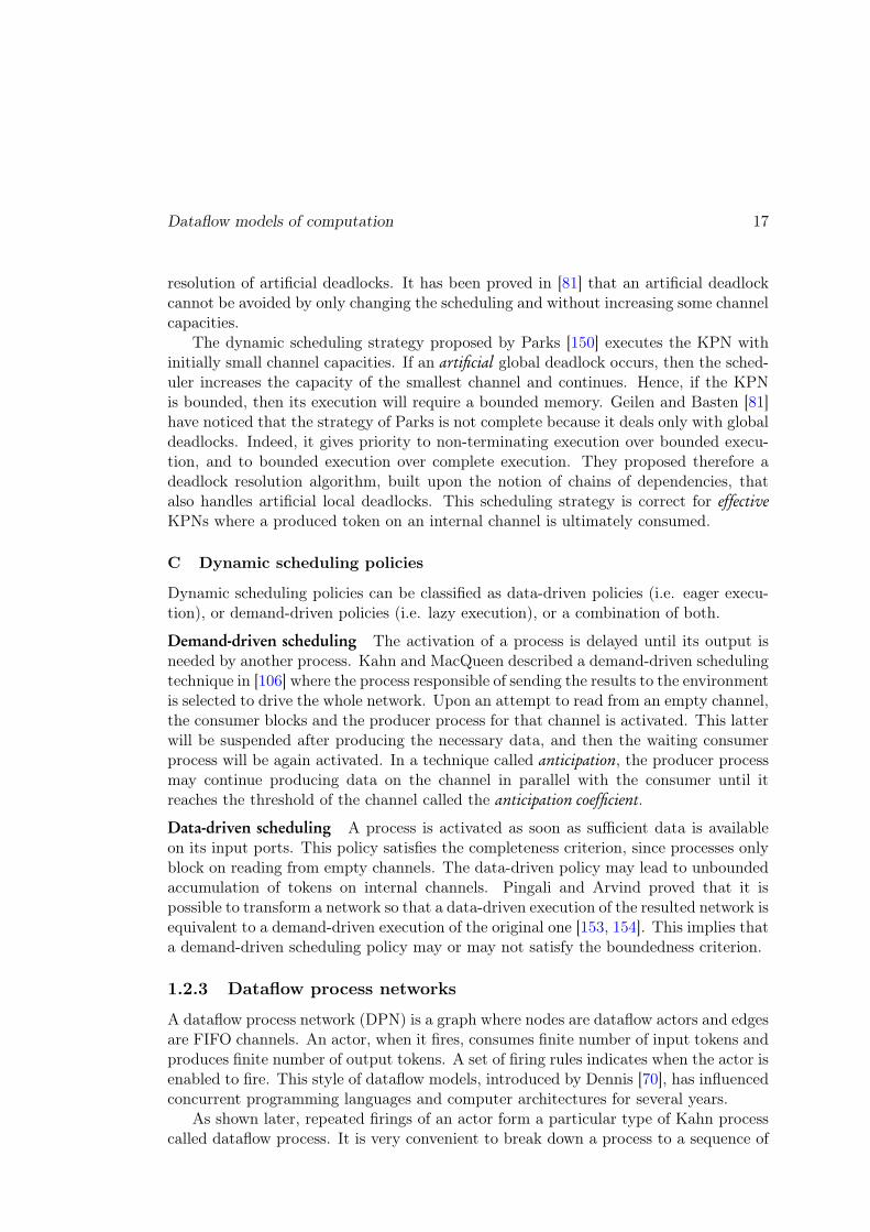
Dynamic scheduling policies can be classified as data-driven policies (i.e. eager execu-tion), or demand-driven policies (i.e. lazy execution), or a combination of both.
Demand-driven scheduling The activation of a process is delayed until its output isneeded by another process. Kahn and MacQueen described a demand-driven schedulingtechnique in [106] where the process responsible of sending the results to the environmentis selected to drive the whole network. Upon an attempt to read from an empty channel,the consumer blocks and the producer process for that channel is activated. This latterwill be suspended after producing the necessary data, and then the waiting consumerprocess will be again activated. In a technique called anticipation, the producer processmay continue producing data on the channel in parallel with the consumer until itreaches the threshold of the channel called the anticipation coefficient.
Data-driven scheduling A process is activated as soon as sufficient data is availableon its input ports. This policy satisfies the completeness criterion, since processes onlyblock on reading from empty channels. The data-driven policy may lead to unboundedaccumulation of tokens on internal channels. Pingali and Arvind proved that it ispossible to transform a network so that a data-driven execution of the resulted network isequivalent to a demand-driven execution of the original one [153, 154]. This implies thata demand-driven scheduling policy may or may not satisfy the boundedness criterion.
1.2.3 Dataflow process networks
A dataflow process network (DPN) is a graph where nodes are dataflow actors and edgesare FIFO channels. An actor, when it fires, consumes finite number of input tokens andproduces finite number of output tokens. A set of firing rules indicates when the actor isenabled to fire. This style of dataflow models, introduced by Dennis [70], has influencedconcurrent programming languages and computer architectures for several years.
As shown later, repeated firings of an actor form a particular type of Kahn processcalled dataflow process. It is very convenient to break down a process to a sequence of

18 Design and Verification
firings in order to enable efficient implementations and formal analyses. However, therelation between the Kahn’s denotational semantics and the operational data-drivensemantics of DPNs became clear only after the outstanding work of Lee and Parks[115, 150, 118].
Mathematically speaking, a dataflow actor with m input and n output channelsconsists of a firing function f : Am −→ An and a finite set R of firing rules. A firingrule is just an m-tuple that is “satisfied” if each sequence of the tuple is a prefix of thesequence of tokens accumulated in the corresponding input channel. In other words,it indicates what tokens must be available at the inputs for the actor to be enabled.The code of the firing function will be executed each time a rule is satisfied, and tokenswill be consumed as specified by that rule. Clearly at most one firing rule should besatisfied at each time in order to have a deterministic behavior of the actor. Therefore,for all r, r′ ∈ R, if r 6= r′, then r ⊔ r′ must not exist.
A set of firing rules is said to be sequential if it can be implemented as a sequenceof blocking read operations. Lee and Parks proposed in [118] a simple algorithm todecide whether a set of firing rules is sequential or not. Sequential firing rules area sufficient condition for a dataflow process to be continuous. Despite the fact thatnot every set of firing rules which satisfies the above mentioned condition about upperbounds is sequential, that condition is more restrictive than what is really necessary fora dataflow to be continuous. A weaker condition (commutative firing rules) is given in[115] which states that if the upper bound r ⊔ r′ exists, then the order in which thesetwo rules are used does not matter; i.e. f(r).f(r′) = f(r′).f(r) and r ⊓ r′ = ǫm. Unlikesequential firing rules, commutative rules enable compositionalilty; in the sense that thecomposition of two actors with commutative firing rules is an actor with commutativefiring rules.
Relation to KPNs
Each actor, with a function f and a set of firing rules R, is associated with a functionalF : [Am −→ An] −→ [Am −→ An] such that
∀g ∈ [Am −→ An] : ∀S ∈ Am : F (g)(S) =
{
f(r).g(S′) if ∃r ∈ R : S = r.S′
ǫm otherwise
As proved in [115], F is a continuous and closed function on the CPO ([Am −→An],⊑) and has therefore a least fixed-point that can be computed iteratively by ∀S ∈Am : g0(S) = ǫn ( g0 is trivially continuous) and gn+1 = F (gn). Clearly, if S = r1.r2. · · · ,then g0(S) = ǫn, g1(S) = f(r1), g2(S) = f(r1).f(r2), . . . In words, the dataflow process(i.e. the least fixed-point) is constructed by repeatedly firing the actor. This leastfixed-point is continuous and it is therefore a Kahn process.
1.2.4 Specific dataflow graph models
Due to Turing-completeness of dataflow graphs, their boundedness and static schedulingare generally undecidable. A bunch of restricted models that trade off expressiveness

Dataflow models of computation 19
for decidability have been developed over the past years. They can be classified intotwo main categories: static dataflow graphs [93] and dynamic dataflow graphs [29].
A Static dataflow graphs
Static dataflow models restrict actors so that on each port and at each firing, they pro-duce and consume a compile-time known number of tokens. These models are amenablefor construction of static schedules (with finite descriptions) that execute the graphs inbounded memory.
The synchronous dataflow (SDF) model [117] is widely used for embedded systemsdesign, especially for digital signal processing systems. In SDF, the production (orconsumption) rate of each port is constant; i.e. an actor produces (or consumes) a fixednumber of tokens on each port. If all the rates in the graph are equal to 1, then thegraph is said to be a homogeneous synchronous dataflow (HSDF) graph. HSDF graphsare equivalent to marked graphs [140] while SDF graphs are equivalent to weightedmarked graphs [187]. Both marked graphs and weighted marked graphs are subclassesof Petri nets, whose literature provides many useful theoretical results. Computationgraphs [109] are similar to SDF graphs; however, each channel is associated with athreshold that can be greater than its consumption rate. An actor can fire only if thenumber of accumulated tokens on each input channel exceeds its threshold. Cyclo-staticdataflow (CSDF) model [41] is a generalization of SDF where the number of produced(or consumed) tokens on a port may vary from one firing to another in a cyclic manner.
The SDF model assumes that both the producer and the consumer of a channelmanipulate the same data type. However, in multimedia applications, it is naturalto use composite data types such as video frames so that, for example, a node mayconsume or produce only a fraction of the frame each time. In the fractional ratedataflow (FRDF) model [146], an actor can produce (or consume) a fractional numberof tokens at each firing which leads generally to better buffering requirements comparedto the equivalent SDF graph. The FRDF model gives a statistical interpretation ofa fraction x
yassociated to a given port in case of atomic data types; i.e. the actor
produces (or consumes) x tokens each y firings but without assuming any knowledgeon the number of tokens produced (or consumed) each time. Therefore, the schedulingalgorithm should consider the worst-case scenarios.
More varieties of the SDF model, that tailor the model for specific needs, can befound in the literature. In the scalable synchronous dataflow model [160], the numberof produced (or consumed) tokens on a given port can be any integer multiple of thepredefined fixed rate of that port. So, all rates of an actor will be scaled by a scalefactor. The static analysis must determine the scale factor of each actor in a way thatcompromises between function call overheads and buffer sizes.
B Dynamic dataflow graphs
Some modern applications have production and consumption rates that can vary at runtime in ways that are not statically predictable. Dynamic models provide the required

20 Design and Verification
expressive power, but at cost of giving up powerful static optimization techniques orguarantees on compile-time bounded scheduling.
Boolean dataflow (BDF) model [48] is an extension of SDF that allows data-dependentproduction and consumption rates by adding two control actors called select and switch.The switch actor consumes one boolean token from its control input and one token fromthe data input, and then copies the data token to the first or second output port accord-ing to the value of the control token. The behavior of the select actor is dual to that ofthe switch actor; both of them combined may allow us to build if-then-else constructsand do-while loops. BDF model is Turing-complete [48]; hence, the questions of bound-edness and liveness are undecidable. Nevertheless, the static analysis is yet possible formany practical problems. A variant of the BDF model is the integer-controlled dataflow(IDF) model [49] in which we can model an actor that consumes an integer token andthen produces a number of tokens equal to that integer.
Scenario aware dataflow (SADF) model [188, 181] extends the SDF model withscenarios that capture different modes of operation and express hence the dynamism ofmodern streaming applications. Production and consumption rates and execution timesof actors may vary from one scenario to another. The SADF model distinguishes dataand control explicitly by using two kinds of actors: kernels for the data processing partsand detectors to handle dynamic transitions between scenarios. Furthermore, there aretwo kinds of channels: control channels which carry scenario-valued tokens and usualdata channels. Detectors contain discrete-time Markov chains to capture occurrencesof scenarios and allow hence for average-case performance analysis.
Parameterized synchronous dataflow (PSDF) [28] and schedulable parametric dataflow(SPDF) [76] models are examples of parameterized dataflow which is a meta-modelingapproach for integrating dynamic parameters (such as parametric rates) in models thathave a well-defined concept of iteration (e.g. SDF and CSDF). SPDF extends SDF withparametric rates that may change dynamically and it is therefore necessary to staticallycheck consistency and liveness for all possible values of the parameters. In addition tothe classical analyses of SDF, we have also to check whether dynamic update of param-eters is safe in terms of boundedness. This analysis is possible since parameters can beupdated only at the boundaries of (local) iterations.
C Comparison of models
Dataflow models can be compared with each other using three features [179]: expressive-ness and succinctness, analyzability and implementation efficiency. These features canbe illustrated by the following examples. BDF model is more expressive than the CSDFmodel since this latter does not allow modeling of data-dependent dynamic productionand consumption rates. The CSDF, SDF, HSDF models have the same expressiveness;any behavior that can be modeled with one of them can be modeled with the two othermodels. Nevertheless, the resulted graphs have different sizes with CSDF graphs be-ing the most succinct. Transformation of (C)SDF graphs into equivalent HSDF graphsuse an unfolding process that replicates each actor possibly an exponential number oftimes [175, 116, 41]. A transformation of CSDF graphs into SDF graphs such that

Dataflow models of computation 21
each CSDF actor is mapped to a single SDF actor was presented in [152]; however, thistransformation may create deadlocks, covers unnecessary computations, and exposesless parallelism.
HSDF model is more analyzable than the (C)SDF model in sense that existinganalysis algorithms for HSDF graphs have lower complexities than the correspondingalgorithms for (C)SDF graphs with the same number of nodes. Implementation ef-ficiency concerns the complexity of the scheduling problem and the code size of theresulting schedules. For example, scheduling of computation graphs is more complexthan scheduling of SDF graphs because of the threshold constraint on consumption.
1.2.5 Dataflow synchronous model
KPNs and Dataflow process networks are closely related, while dataflow synchronousmodels are quite different. There are a bunch of synchronous languages (e.g. SIG-
NAL [92], ESTEREL [24], LUSTRE [95], LUCID SYNCHRONE [54]) dedicated to reactivesystems design that rely on the same assumptions (the synchronous paradigm) [19, 20]:
1. Programs progress via an infinite sequence of reactions. The system is viewedthrough the chronology and simultaneity of the observed events, which constitute a logi-cal time, rather than the chronometric view of the execution progress. The synchronoushypothesis therefore assumes that computations and communications are instantaneous.This hypothesis is satisfied as long as a reaction to an input event is fast enough to pro-duce the output event before the acquisition of the next input events. The synchronyhypothesis simplifies the system design; however it implies that only bounded KPNscan be specified (by programming processes that act as bounded buffers).
2. Testing inputs for emptiness is allowed. Hence, decisions can be taken on thebasis of the absence of some events. Synchronous programs can have therefore a non-deterministic behavior.
3. Parallel composition is given by taking the pairwise conjunction of associatedreactions, whenever they are composable.
A Abstract clocks
The denotational semantics of both untimed models of computation (e.g. KPNs) andtimed models (e.g. dataflow synchronous model) can be expressed in a single denota-tional framework (“meta-model”): the tagged signal model [119]. The main objectivesof this model is to allow comparison of certain properties of several models of com-putation, and also to homogenize the terms used in different communities to meansometimes significantly different things (e.g. “signal”, “synchronous”). The basic idea ofthis framework is to couple streams (or sequences) with a tag system and consider hencesignals instead of untimed streams. The tag system, when specifying a system, shouldnot mark physical time but should instead reflect ordering introduced by causality. Thetag system presented in this section is tailored to the dataflow synchronous model.
Definition 1.1 (Tag system). A tag system is a complete partial order (T ,⊑). Itprovides a discrete time dimension that corresponds to logical instants according to

22 Design and Verification
which the presence and absence of events can be observed.
Definition 1.2 (Events, Signals). An event is a pair (t, a) ∈ T × A such that A isa value domain. A signal s is a partial function s : C ⇀ A with C a chain in T . Itassociates values with totally ordered observation points.
Definition 1.3 (Abstract clock). The abstract clock of a signal s : C ⇀ A is itsdomain of definition s = dom(s) ⊆ C.
Usual set operations and comparisons can be naturally applied on clocks. Relationsbetween clocks can be deduced from the different operations on signals (e.g. merge,select). The relational synchronous language SIGNAL allows explicit manipulation ofclocks. Table 1.1 shows the essential SIGNAL operators and what relations should relateclocks. Both the select and merge operators are not Kahn processes. Unlike LUSTRE
and ESTEREL, SIGNAL is a multi-clocked model; i.e. a master clock is not needed inthe system. Therefore, two signals may have totally unrelated abstract clocks; such asthe operands of the merge process.
Construct clock relations semanticsStepwise extensions
r = f(s1, . . . , sn)r = s1 = · · · = sn ∀t ∈ r : r(t) = f(s1(t), . . . , sn(t))
Delay
r = s$ init a0r = s
∀t ∈ r : r(t) ={
a0 if t =dr
s(t−) otherwise
t− and t are successive tags in rSelect
r = swhen br = s ∩ {t ∈ b|b(t) =true}
∀t ∈ r : r(t) = s(t)
Merge
r = s1 default s2r = s1 ∪ s2 ∀t ∈ r : r(t) =
{
s1(t) if t ∈ s1s2(t) otherwise
Table 1.1: SIGNAL elementary processes
Elementary relations can be combined to produce more sophisticated clock trans-formations. One important clock transformation is the affine transformation, describedin [168], and used extensively in this thesis. A subclass of affine relations between ab-stract clocks was used in [79] to address time requirements of streaming applications onmultiprocessor systems on chip.
Definition 1.4 (Affine transformation). An affine transformation of parameters (n, ϕ, d)applied to the clock s produces a clock r by inserting (n− 1) instants between any twosuccessive instants of s, and then counting on this fictional set each dth instant, startingwith the (ϕ+ 1)th instant.
B Quasi-synchrony and N-synchronous
Two signals s1 and s2 are said to be synchronous if and only if s1 = s2. Synchronousdataflow languages provide a type system, called clock calculus, that ensures that a signal

Dataflow models of computation 23
can be assigned only to another signal with the same clock (i.e. buffer-less communi-cation). This does not however mean that a signal cannot be delayed. Mitigation ofthis strong requirement has been the subject of some works motivated by the currentpractice in real-time systems development; especially real-time systems that consist ofa set of periodic threads which communicate asynchronously.
Quasi-synchrony is a composition mechanism of periodic threads that tolerates smalldrifts between thread’s release (i.e. activation) clocks [53]. If s and r are the activationclocks of two periodic threads, then their quasi-synchronous composition is such thatbetween two occurrences of s there are at most two occurrences of r, and conversely,between two occurrences of r there are at most two occurrences of s. This definitionwas refined in [96] to enable synchronous occurrences. If t1 and t2 are two successivetags in s, then |{t ∈ r|t1 ❁ t ⊑ t2}| ≤ 2; Conversely, if t1 and t2 are two successivetags in r, then |{t ∈ s|t1 ❁ t ⊑ t2}| ≤ 2. A stream between two quasi-synchronouslycomposed threads can be no more considered neither as an instantaneous (buffer-less)communication nor as a bounded FIFO; but rather as a shared variable. Hence, somevalues are lost if the sender is faster than the receiver and some values are duplicatedif the receiver is faster than the sender. This non-flow-preserving semantics was takenfurther in the Prelude compiler [149] as shown later.
In the N-synchronous paradigm [62], two signals can be assigned to each other aslong as a bounded communication is possible. Hence, the new synchronizability relationstates that two clocks s and r are synchronizable if and only if for all n ∈ N>0, the nth
tags of s and r are at bounded distance. Formally, ∀t′ ∈ s : |{t ∈ s|t ⊑ t′}| − |{t ∈r|t ⊑ t′}| is bounded. This model allows to specify any bounded KPN. Unlike thequasi-synchronous approach, communications in this model are flow-preserving.
C From synchrony to asynchrony
Although the synchronous hypothesis states that reactions are instantaneous, causalitydependencies dictate in which order signals are evaluated within a reaction. For in-stance, the presence of a signal must be decided before reading its value. A schizophreniccycle is one in which the presence of a signal depends on its value. More dependenciescan be deduced from elementary processes. For example, computing values of s1, . . . , snmust precede computing value of r = f(s1, . . . , sn). Synchronous languages provide thenecessary tools to check deadlock freedom; that is, there is no cycle in the dependenciesgraph.
Desynchronizing a signal to obtain an asynchronous communication consists in get-ting rid of the tags information and hence preserving only the stream. A synchronousprocess may take some decisions based on the absence of a signal; but it can no moretest the emptiness of an input in an asynchronous implementation. The question thatraises naturally is whether it is possible to resynchronize a desynchronized signal. Anendochronous process [19] is a process that can incrementally infer the status (pres-ence/absence) of all signals from already known and present signals. Therefore, anendochronous process should have a unique master clock so that all the other clocks aresubsets of it. Endochrony is undecidable in the general case [19]. An endochronous pro-

24 Design and Verification
cess is equivalent to a dataflow process with sequential set of firing rules; and it is hencea Kahn process. Weak endochrony [157] is a less restrictive condition than endochrony.A weakly endochronous process is equivalent to a dataflow process with commutativefiring rules. Similarly to composition properties of dataflow actors, the compositionof two endochronous processes is not in general an endochronous process; while thecomposition of two weakly endochronous processes results in a weakly endochronousprocess.
The compositional property of isochrony ensures that the synchronous compositionof (endochronous) processes is equivalent to their asynchronous composition. It is animportant property for designing globally asynchronous locally synchronous (GALS)architectures. Roughly speaking, a pair of processes is isochronous if every pair of theirreactions which agree on present common signals also agree on all common signals.
D Lucy-n
Lucy-n [134] is an extension of the synchronous language LUSTRE with an explicit bufferconstruct for programming networks of processes communicating through boundedbuffers. The synchronizability relation is the one defined by the N-synchronous paradigm.Lucy-n provides a clock calculus (defined as an inference type system) which can com-pute the necessary buffer sizes using a linear approximation of boolean clocks. Weillustrate the semantics of Lucy-n using a simple example (Listing 1.1). The clock ofeach signal is denoted by a binary sequence such that 1 represents presence and 0 rep-resents absence. The clock calculus handles only ultimately periodic clocks which aredenoted syntactically by u(v). The N-synchronous execution is presented in Table 1.2.
Listing 1.1: Example in Lucy-n.
let node example x=y where
rec a=x when (0 1)and b=x when (1 0 1)and y= a+ buffer(b)
example
when
when
Since the (+) operator is a stepwise operator, signals a and buffer(b) must havethe same clock 1ω on (0 1)ω. However, this program must be rejected because signal aand b are not synchronizable (as defined by the N-synchronous paradigm). Indeed, thedifference between the nth tags of a and b are not at a bounded distance when n tendsto infinity. So, the inserted buffer is unbounded.
Table 1.2: N-synchronous execution of Program 1.1.
signal flow clockx 2 5 1 0 3 2 1 1ω
a = x when (0 1) 5 0 2 1ω on (0 1)ω
b = x when (1 0 1) 2 1 0 2 1 1ω on (1 0 1)ω
buffer(b) 2 1 0 1ω on (0 1)ω
y 7 1 2 1ω on (0 1)ω

Dataflow models of computation 25
E Prelude
Prelude [149] is a real-time programming language build upon the synchronous languageLUSTRE. Listing 1.2 represents a simple example; while Table 1.3 shows its semantics.The difference between Prelude and the synchronous languages consists mainly in thetwo following points.
Listing 1.2: Example in Prelude.
node foo (x: rate(10,0) ) returns (y)var a,b;
let
(y, a) =Add (x, (1 fby b)∗2);
b = INC(a/2);tel
foo
INC
ADD
Table 1.3: Semantics of Program 1.2.
date 0 10 20 30 40 50 60x 3 2 4 1 0 6 2a 4 3 9 6 10 16 13a/2 4 9 10 13b 5 10 11 14
1 fby b 1 5 10 11(1 fby b)∗2 1 1 5 5 10 10 11
Real-time constraints: Real-time constraints represent environmental constraints andthey are specified either on node inputs and outputs (e.g. periods, phases, deadlines)or on nodes (worst-case execution time). In Listing 1.2, signal x has a period of 10and a first start time equals to zero. This implies that task ADD is a periodic taskwith a period equal to 10. The compiler checks the consistency of real-time constraints(e.g. inputs and outputs of a node have the same period) and earliest-deadline firstschedulability of the specification.
Communication patterns: Rate transition operators (e.g. ∗, /) handle transition be-tween nodes of different rates and hence enable the definition of user-provided commu-nication patterns. For example, in Listing 1.2, flow a is under-sampled using operator/2; which implies that node ADD is twice as fast as node INC. As in quasi-synchrony,communication is non-flow-preserving; i.e. when the producer is faster than the con-sumer, an adapter is added allowing some produced tokens to not be buffered; andwhen the consumer is faster, an adapter is added to allow for reading the same valueseveral times. Furthermore, communications are deterministic (i.e. not affected by theearliest-deadline first scheduling policy and preemption). To realize this objective somedeadlines are adjusted to enforce some precedences between jobs.

26 Design and Verification
1.3 Static analysis of (C|H)SDF graphs
The HSDF, SDF, and CSDF models have been used as the underlying models of severalDigital Signal Processing (DSP) programming environments, since they combine goodlevels of analyzability and expressivity. Indeed, properties such as boundedness andliveness are decidable. Furthermore, static-periodic scheduling of (C|H)SDF graphshas been the subject of an enormous number of works that have addressed the problemwith respect to different non-functional constraints: throughput, buffering, latency, codesize, etc. The proposed analyses abstract from the actual values of data that are beingcommunicated, and focus only on the non-functional properties such as the distributionof tokens over channels. This section presents some existing analyses; and it is by nomeans a complete in-depth survey.
Definition 1.5 (Static dataflow graph). A static dataflow graph is a directed graphG = (P,E) consisting of a finite set of actors P = {p1, . . . , pN} and a finite set of one-to-one edges (or channels) E. A channel e = (pi, pk, x, y) ∈ E connects the producer pito the consumer pk such that the production (resp. consumption) rate is given by theinfinite integer sequence x ∈ Nω (resp. y ∈ Nω). For instance, the jth firing of actor pi(denoted by pi[j]) writes x(j) tokens on channel e.
(H|C)SDF graphs are specific cases of static dataflow graphs. Each rate functionx is a constant sequence (i.e. x = aω with a ∈ N>0) in the SDF model, a periodicsequence (i.e. x = vω with v ∈ N∗ and ‖v‖ > 0) in the CSDF model, and equals to 1(i.e. x = 1ω) in the HSDF model. Figure 1.1 shows a SDF graph, and its transformationinto an equivalent HSDF graph, where a black dot on an edge represents an initial tokenin the channel.
(a) (b)
Figure 1.1: Example of (a) a cyclic SDF graph, and (b) its equivalent HSDF graph.
1.3.1 Reachability analysis
Since SDF graphs are equivalent to weighted marked graphs, many techniques from thePetri nets literature can be used to analyze them. A marking M (or channels state)is denoted by a vector whose ith component M(i) represents the number of tokens in

Static analysis of (C|H)SDF graphs 27
channel ei. The initial marking M0 contains for each channel e its number of initialtokens θ(e). Figure 1.2 represents the reachability graph of the SDF example (Figure1.1(a)) where states are markings and transitions are actor firings. The SDF exampleis strictly bounded since its reachability graph is finite. However, if we delete channele1, then the reachability graph is infinite since actor p1 is always enabled. This impliesthat the new SDF graph is not strictly bounded; but it is bounded since there exists atleast one complete execution with bounded channels.
A dataflow graph is live if it has executions in which all actors are fired infinitely.An immediate result of the functional determinism of CSDF graphs (i.e. the schedulingorder does not affect the results) is that if one execution deadlocks then all executionsdeadlock [84]. The reachability graph in Figure 1.2 is deadlock-free (i.e. ∀M : ∃pi ∈ P :pi is firable at M) and live (i.e. ∀pi : ∀M : ∃M ′ : the firing sequence that transforms Minto M ′ contains pi). If θ(e2) = 1, then the SDF graph is not live because [0 1 1]T
p3−→[2 1 0]T
deadlock−→ .
Figure 1.2: Reachability graph of the SDF example.
A Consistency
If a dataflow graph is not consistent, then its execution requires unbounded channelsor unbounded number of initial tokens to not deadlock. Only consistent graphs are ofinterest in this thesis. Consistency is a structural property that can be verified efficiently[17, 117, 41]. A (C|H)SDF graph can be described by a |E| × |P | topology matrix Γ
such that ∀ej = (pi, pk, vω1 , v
ω2 ) : Γj,i =
‖v1‖|v1| ,Γj,k = −‖v2‖
|v2| , and Γj,l = 0 for any otheractor pl.
For a graph to be consistent, a positive non-null integer solution of the balanceequation (Equation 1.1) must exist.
Γ~r = ~0 (1.1)
The minimal solution is called the repetition vector which determines the relative firingfrequencies of actors. The repetition vector of the SDF graph in Figure 1.1 is equal to[2 1 3]T.
The balance equation can be easily explained as follows. Let |σ|i be the number offirings of actor pi during a complete execution σ. The total number of produced tokens

28 Design and Verification
on channel e = (pi, pk, vω1 , v
ω2 ) converges to ‖v1‖
|v1| |σ|i while the number of consumed
tokens converges to ‖v2‖|v2| |σ|k. A necessary condition for e to be bounded is that
|σ|i|σ|k
=‖v2‖|v2|
|v1|‖v1‖
=~r(i)
~r(k)
Equation 1.1 ensures that cycles can satisfy this constraint. Any dataflow graph withoutundirected cycles is consistent.
B Graph iteration
An iteration is a sequence of actor firings that returns the graph into its initial marking.The firing sequence must contain k~r(i) firings of each actor pi with k ∈ N>0. Repeatingthe iteration infinitely results in a bounded and complete execution. For the reachabil-ity graph in Figure 1.2, the periodic sequence (p2 p3 p3 p3 p1 p1)
ω is such a boundedexecution. Not all bounded executions should be periodic. Indeed, the language recog-nized by the reachability graph in Figure 1.2 (considered as a Büchi automaton) is notperiodic.
The balance equation is a necessary but not sufficient condition for the existenceof an iteration. In fact, an iteration that returns the graph to its initial markingmay not exist. That depends essentially on the initial marking. If the graph is liveand consistent, then an iteration always exists [84]. One simple solution to test theexistence of an iteration is through simulated execution that consists in constructingthe reachability graph [117]. A second solution is to check that all maximal stronglyconnected components are deadlock-free [84]. The third solution consists in checkingthat the equivalent HSDF graph of any directed cycle in the CSDF graph is live [41]. Anecessary and sufficient condition for a single-rate (i.e. HSDF) graph to be live is thatevery directed cycle in it contains at least one initial token.
A sufficient and necessary condition for a cycle to be deadlock-free was presentedfor computation graphs in [109], and adapted for SDF graphs in [141]. A cycle {e2 =(p1, p2, a
ω1 , b
ω2 ), . . . , e1 = (pn, p1, a
ωn , b
ω1 )} deadlocks if and only if the following integer
program has a non-negative integer solution.
Γ~x ≤ ~B
where Γ is the topology matrix of the cycle and ~B is the vector such that ~B(i) =bi− θ(ei)−1. Assume that there is a non-negative integer solution ~x0. After firing eachactor pi as many times as indicated by ~x0(i), the number of tokens in channel ei willbe less or equal to θ(ei) + ~B(i) = bi − 1. This is a deadlocked state.
In the periodic schedule (p2 p3 p3 p3 p1 p1)ω, three instances of actor p3 are enabled
at the same time. Therefore, if there are enough processing units, the three firings canbe executed in parallel. This behavior is called auto-concurrency. To constrain theauto-concurrency of an actor p such that at most b firings of actor p can execute inparallel, we need to add a single-rate self-loop e = (p, p, 1ω, 1ω) such that θ(e) = b. InFigure 1.1, auto-concurrency of actors p1 and p3 is disabled in the HSDF graph.
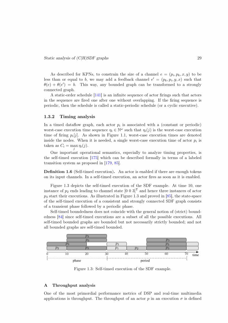
Static analysis of (C|H)SDF graphs 29
As described for KPNs, to constrain the size of a channel e = (pi, pk, x, y) to beless than or equal to b, we may add a feedback channel e′ = (pk, pi, y, x) such thatθ(e) + θ(e′) = b. This way, any bounded graph can be transformed to a stronglyconnected graph.
A static-order schedule [141] is an infinite sequence of actor firings such that actorsin the sequence are fired one after one without overlapping. If the firing sequence isperiodic, then the schedule is called a static-periodic schedule (or a cyclic executive).
1.3.2 Timing analysis
In a timed dataflow graph, each actor pi is associated with a (constant or periodic)worst-case execution time sequence ηi ∈ Nω such that ηi(j) is the worst-case executiontime of firing pi[j]. As shown in Figure 1.1, worst-case execution times are denotedinside the nodes. When it is needed, a single worst-case execution time of actor pi istaken as Ci = max
jηi(j).
One important operational semantics, especially to analyze timing properties, isthe self-timed execution [175] which can be described formally in terms of a labeledtransition system as proposed in [179, 85].
Definition 1.6 (Self-timed execution). An actor is enabled if there are enough tokenson its input channels. In a self-timed execution, an actor fires as soon as it is enabled.
Figure 1.3 depicts the self-timed execution of the SDF example. At time 10, oneinstance of p2 ends leading to channel state [0 0 3]T and hence three instances of actorp3 start their executions. As illustrated in Figure 1.3 and proved in [85], the state-spaceof the self-timed execution of a consistent and strongly connected SDF graph consistsof a transient phase followed by a periodic phase.
Self-timed boundedness does not coincide with the general notion of (strict) bound-edness [84] since self-timed executions are a subset of all the possible executions. Allself-timed bounded graphs are bounded but not necessarily strictly bounded; and notall bounded graphs are self-timed bounded.
time
periodphase
Figure 1.3: Self-timed execution of the SDF example.
A Throughput analysis
One of the most primordial performance metrics of DSP and real-time multimediaapplications is throughput. The throughput of an actor p in an execution σ is defined

30 Design and Verification
as the average number of firings of p in σ per unit of time; and it is denoted by Θ(p, σ).The maximum throughput of an actor p is obtained by the self-timed execution; and itis denoted simply by Θ(p). The self-timed throughput of an actor in a consistent andstrongly connected CSDF graph is bounded; However, if an actor is always enabled, thenits self-timed throughput tends to infinity. The self-timed throughput of a consistentand strongly connected graph G is defined as Θ(G) = Θ(pi)
~r(i) for an arbitrary pi ∈ P .Throughput analysis has been proposed in the literature either as a (symbolic)
state-space exploration [85, 84] or as a maximum cycle mean analysis [175]. In the firstapproach, the self-timed throughput is computed from the periodic phase of the self-timed execution constructed by a simulated execution. In the second approach, and asproved in [175], the self-timed throughput of the graph is equal to 1 over the maximumcycle mean (MCM) of the equivalent HSDF graph. The MCM of a HSDF graph G,assuming that ηi is a constant sequence for all pi ∈ P , is defined as
MCM(G) = maxcycle C∈G
∑
pi∈PCi
∑
e∈Cθ(e)
Efficient algorithms for computing MCM have been proposed in the literature [108,64]. However, transforming a CSDF graph into a HSDF graph can result in an expo-nential number of actors compared with the original graph. Because of this, and asillustrated by experimental evaluations [85], state-space exploration approach outper-forms the MCM-based approach.
Reduction techniques [80] may help to obtain smaller and hence more analyzableHSDF graphs. One proposed technique is to abstract a (H)SDF graph G with a smallerone G′ where actors with identical firing rates are ordered and represented as a singleactor. Authors proved that, following their transformation rules, the resulted graphG′ will have a conservative throughput; i.e. Θ(G′) ≤ Θ(G). A second technique wasa new transformation algorithm of SDF graphs into HSDF graphs that produces notnecessarily an equivalent image but only a conservative one. This technique relies on asymbolic state-space exploration (a Max-Plus model) limited to the phase and a periodof the self-timed execution. The resulted graph is at most quadratic in the number ofinitial tokens in the original graph.
As shown in [85, 68], the state-space exploration can be characterized by a Max-Plus algebra [7]. Let ti[j] be the start time of the jth firing of actor pi. In Max-Plusalgebra, ti[j] is expressed in terms of the start times of some preceding firings by meansof two operators: the maximum ⊕ (used in the role of addition) and the ordinaryaddition ⊗ (used in the role of multiplication). For the HSDF example (Figure 1.1(b)),t1,1[j] = (t1,2[j − 1]⊕ 10)⊕ (t3,1[j]⊗ 20)⊕ (t3,2[j]⊗ 20). The max-plus time system ofa SDF graph can be constructed without transforming the graph into an HSDF graph(see [68] for details). The set of sum-of-products equations can be encoded as a matrixequation
~tj = A~tj−1
Vector ~tj describes the start times of the jth firings of all actors; i.e. ∀pi : ~tj(i) = ti[j].

Static analysis of (C|H)SDF graphs 31
If ~t0 encodes the initial state, then ~tj = Aj~t0 describes the progress of the self-timedexecution over time. The eigenvalue λ (i.e. the solution of equation A~t = λ⊗~t ) equalsthe MCM of the graph; and thus the throughput of the graph is equal to 1
λ.
A parametric throughput analysis of SDF graphs is presented in [83] where actors’execution times can be parameters. The throughput is hence computed as functionof the parameters. Recalculation of throughput is then simply an evaluation of thisfunction for specific parameter values. This parametric analysis could be useful atdesign time to avoid recalculation of the throughput for each different configuration.
B Throughput in multiprocessor scheduling
The self-timed execution, under which a maximal throughput can be obtained, assumesthat there is an unlimited number of processing units. Multiprocessor scheduling ofdataflow graphs assumes a fixed number of processing units. It can be either dynamicor static [114, 175]. The partitioned static-order scheduling problem of dataflow graphsconsists in statically (and permanently) mapping actors onto a fixed number of pro-cessors {A1, . . . , AM} (the allocation step), constructing a static-order schedule of eachpartition Ai (the scheduling step), and determining exactly when each actor fires suchthat all data precedence constraints are met (across processors). This problem has beenextensively studied in the two past decades from multiple angles of view. Throughputmaximization was one of the most important optimization criteria. Existing solutionseither transform the graph into a HSDF graph [175, 176, 139] or compute mapping andscheduling directly on (C)SDF graphs [183, 42].
The achieved throughput depends on both allocation and scheduling. In most ap-proaches the two steps are performed separately as a bin-packing heuristic due to theNP-hardness of the scheduling problem. Firstly, the actors are ordered according tosome criterion. In [183], actors are ordered according to their impact on the through-put of the graph. As described before, the throughput of the graph is limited by itscritical path. To avoid graph transformation and MCM analysis, authors proposed anapproximate cost function to estimate the criticality of an actor pi.
cost(pi) = maxCycle C|pi∈C
∑
pk∈C~r(k) . avg(ηk)
∑
e∈Cθ(e)/e
avg(ηk) is the average execution time of actor pk on different processing units. Fora channel e = (p, q, x, vω), value e is equal to ‖v‖
|v| . After ordering the actors, thesecond step in the heuristic consists in binding actors, one after another, to processorsaccording to some objective function. In [183, 139], the objective was to balance theload of partitions. The load of a partition is estimated by the processor, memory, andconnection utilizations. Actors are then assigned to partitions with a first fit or best fitstrategy to achieve the desired objective.

32 Design and Verification
C Retiming technique
Besides the graph topology and execution times, the initial delay distribution maylimit the throughput. Retiming is a graph transformation technique for performanceoptimization (e.g. throughput maximization, minimizing memory usage, decreasingpower consumption, etc.) that redistributes the delays and does not affect neither thetopology nor the functionality of the graph [128, 199, 198, 191, 148, 122].
Figure 1.4(a) shows the SDF example with a different initial delay distribution(θ(e1) = 4, θ(e2) = 0, and θ(e3) = 2). We impose that during each period of the self-timed execution, every actor pi fires only ~r(i) times (we can model this constraint byadding a fictional actor as illustrated in Figure 1.4(a)). As can be deduced from theself-timed execution (Figure 1.4(c)), the self-timed throughput is equal to 1
60 . Afterretiming the graph (θ(e1) = 0, θ(e2) = 2, and θ(e3) = 1), the new self-timed throughputis equal to 1
40 (Figure 1.4(b)).
(a) CSDF graph
timeperiod
(b) Self-timed execution after retiming. Θ(G) = 1/40.
timeperiod
(c) Self-timed execution. Θ(G) = 1/60.
Figure 1.4: Retiming of a SDF graph.
Let G be a consistent and live SDF graph and ~z : P −→ Z be a transformation vectorsuch that the new retimed graph is obtained by firing each actor pi in the original graph~z(i) times. Hence, for very channel e = (pi, pk, v
ω1 , v
ω2 ), the new number of initial tokens
is θ′(e) = θ(e) + ‖v1‖~z(i)− ‖v2‖~z(k). The retiming vector in the previous example was[2 0 1]T. A retiming is legal if it results in nonnegative delay distribution. The retimedgraph will be then bounded and live. Most solutions search for an optimal legal retimingor a feasible one that satisfies some throughput constraints.
D Latency analysis
Another useful performance metric of interactive concurrent real-time applications islatency. Latency was defined in [175] for HSDF graphs and consistently generalized in

Static analysis of (C|H)SDF graphs 33
[86] to SDF graphs. It is measured for two actors pi and pk that are usually consideredas the input and output of the system. To measure the latency, two fictional actors p0and pN+1 will be added to the graph such that in each iteration of the graph (accordingto the repetition vector) these two actors fire only once (i.e. ~r(0) = ~r(N + 1) = 1).The fictional actors have null execution times (i.e. η0 = ηN+1 = 0ω) in order to notaffect the timing analysis. Two channels are added to the graph: e = (p0, pi, ~r(i)
ω, 1ω)and e′ = (pk, pN+1, 1
ω, ~r(k)ω) with θ(e) = θ(e′) = 0. The κ(j)th firing of pN+1 isthe firing that consumes some tokens whose construction involves the reading of sometokens produced by the jth firing of actor p0. Hence, the latency of actors pi and pk inan execution σ is given as
Lσi,k = maxj∈N>0
{tN+1[κ(j)]− t0[j]}
where ti[j] is the start time of firing pi[j]. The minimal latency is obtained by theself-timed execution. However, due to resource constraints, the self-timed executioncould not be possible. The worst minimal achievable latency is obtained for a singleprocessor.
1.3.3 Memory analysis
Memory analysis concerns the minimization of both code size and channel sizes. Memoryconstraints are strong non-functional requirements since the amount of on-chip memoryin embedded systems is severely limited due to several constraints (e.g. cost, powerconsumption, speed penalties, etc.).
A Code size minimization
Automatic code generation is an essential feature of any dataflow-based design environ-ment. One widely used code generation strategy in single-processor scheduling is calledthreading which inlines the code of actors in a static-periodic schedule. One objective ofsuch strategy is to minimize the resulted code size by using loops as efficient as possible.For the schedule (p2 p3 p3 p3 p1 p1)
ω of the SDF example, the generated code is shownin Listing 1.3.
Listing 1.3: Software synthesis from the SDF example.
while(true) do{
code of p2for(i=0;i<3;i++){ code of p3 }
for(i=0;i<2;i++){ code of p1 }
}
As shown in the reachability graph of the SDF example, there is an infinite numberof static-periodic schedules that may have different code sizes. Periodic schedules thatcan be described with a regular expression in which each actor appears only once, andhence have a minimal size, are called single appearance schedules [30, 33]. The previous

34 Design and Verification
example is a single appearance schedule that can be described with (p2(p3)3(p1)
2)ω. Ashas been proved, every consistent acyclic SDF graph has at least one single appearanceschedule. More results can be found in [32, 17, 31]. For instance, a SDF graph hasa single appearance schedule if and only if each strongly connected component has asingle appearance schedule. Furthermore, a consistent strongly connected SDF graphhas a single appearance schedule if and only if all its strongly connected subgraphs areloosely interdependent. As an illustration, the SDF example is loosely interdependentbecause it can be partitioned into two subsets A = {p2} and B = {p1, p3} such thatactors in subset A can fire, as many times as indicated by the repetition vector, beforeany firing of actors in subset B. If the delay distribution is such that ∀i : θ(ei) = 1, thenthe SDF example is not loosely interdependent; a single appearance schedule does nothence exist. Since a graph may have multiple single appearance schedules, selecting theone with the least buffering requirements was the choice of most solutions [143, 145].
B Buffer minimization
Minimizing buffer storage capacity has been the subject of several heuristics and exactapproaches in the last two decades. It consists in finding the smallest buffering require-ments that allow for a complete execution. The buffer minimization problem is knownto be NP-complete [17, 141] by reduction of the Feedback arc set problem to bufferminimization in HSDF graphs.
If channels are implemented as separated storage spaces (i.e. empty space in onechannel cannot be used to store tokens of other channels), then the buffer minimizationproblem consists in finding a schedule that minimizes
∑
e∈E(e)max
t{θt(e)} where θt(e) is
the number of tokens in channel e at time t and (e) is the size of a token (deduced fromthe data type). From the reachability graph of the SDF example and assuming that alltokens in the graph have the same size, the periodic schedule (p3 p2 p3 p1 p3 p1)
ω resultsin the smallest buffer size distribution [4 2 3]T. This distribution is indeed minimalbecause the lower bound of the size of a channel e = (pi, pk, a
ω, bω) in a SDF graphthat can be achieved by any valid schedule is given in [141] by a+ b− gcd(a, b) + θ(e)mod gcd(a, b) if 0 ≤ θ(e) ≤ a+ b−gcd(a, b), and by θ(e) otherwise. This first variationof the buffer minimization problem is considered, for instance, in [132, 91, 63, 1].
If memory is shared between buffers (i.e. all buffers share a single storage space),then the buffer minimization problem consists in finding the schedule that minimizesmaxt{∑e∈E
(e)θt(e)}. Unlike the previous variation, this latter approach, considered in
[142], must take into account the lifetime of tokens. Hybrid methods may combine thetwo variations as proposed in [147, 82]. In case the smallest buffer size distributionis not unique, scheduling algorithms choose either the distribution with the highestthroughput or the one with the smallest code size.
Another variation of the buffer minimization problem is to minimize the buffering re-quirements while satisfying a throughput constraint [194, 195, 18]. Indeed, the schedulewith minimal buffer sizes may have a throughput that does not satisfy timing con-straints. Figure 1.5 shows, for each total amount of buffering requirements, the buffer

Real-time scheduling 35
size distribution that gives the highest self-timed throughput. For example, if the totalstorage space is constrained to be at most 10, then there are two buffer size distributions([5 2 3]T and [4 2 4]T) which achieve the best self-timed throughput (0.014). Since theSDF example is strictly bounded, the maximal throughput that can be achieved witha bounded storage distribution is the one computed by the MCM analysis. The set ofall trade-offs between the distribution size and the throughput is called the Pareto spaceof throughput and storage trade-offs. A technique that compute either the exact or theapproximate Pareto space of (C)SDF graphs was presented in [184, 180].
Storage distribution size
Th
rou
gh
pu
t
Figure 1.5: Pareto space of the SDF example.
1.4 Real-time scheduling
The inflexibility and difficult maintainability of systems scheduled by cyclic executives(i.e. static-order schedules) led to the development of new real-time scheduling theoriessuch as priority-driven scheduling theory. Much effort has been devoted to identifymodels of systems, such as the periodic task system model of Lui and Layland [127],from the requirements encountered in the development of real-time systems. Besidesmodels, many theoretical results have been established to predict before the costlyimplementation phase whether the system will meet its timing requirements even in theworst-case scenarios.
Current models are much mature and general [165, 66, 51, 74]; they consist ofperiodic, sporadic, and aperiodic tasks (i.e. threads) with implicit deadlines (deadlinesequal to periods), constrained deadlines (deadlines less than or equal to periods), orarbitrary deadlines. More requirements are considered such as jitters, resource accessprotocols, precedence constraints, etc. However, some models are well understood thanothers. For instance, aperiodic tasks are less predictable than periodic and sporadictasks. In this section, we will consider a restricted but yet expressive task model thatcorresponds to our needs for a priority-driven scheduling of dataflow graphs.

36 Design and Verification
1.4.1 System models and terminology
A real-time system comprises a set of N tasks (a task set) P = {p1, p2, . . . , pN}, eachtask consists of an infinite or finite sequence of jobs (invocations, activations, or re-quests). The jth job of task pi is denoted by pi[j]. A job executes in a sequentialfashion and does not self-suspend. In addition, auto-concurrency is not allowed andtasks are independent and do not share any resources (except the processors of course)unless it is stated otherwise. A run-time scheduler (dispatcher or operating system)controls which job is executing at a given moment on a given processor.
Timing constraints are of a particular interest in real-time computing. In the pre-sented model of computation, timing constraints are expressed in terms of deadlines. IfRi[j] is the release (or arrival) time of job pi[j] and di is the relative deadline of task pi,then job pi[j] meets its timing constraint if its execution completes before the absolutedeadline Di[j] = Ri[j] + di. As we mentioned before, deadlines can be either hard orsoft.
Scheduling theory generally assumes three kinds of tasks, characterized by the arrivalpattern of their jobs.
• Periodic tasks. Jobs of a periodic task pi arrive at fixed intervals; i.e. ∀j ∈ N>0 :Ri[j+1] = Ri[j]+πi. The constant πi is called the period of the task. This arrivalpattern is thus time-driven. A periodic task pi is characterized by a worst-caseexecution time Ci, a hard deadline di, and a first release time (called phase oroffset) ri = Ri[1].
• Aperiodic tasks. Jobs of an aperiodic task arrive randomly, usually in response tosome external triggering event. This arrival pattern is thus event-driven. Besideshaving unknown interarrival time of requests, aperiodic tasks have unknown (orextremely large) worst-case execution times. Due to this unpredictability, aperi-odic tasks can have only soft deadlines.
• Sporadic tasks. A sporadic task pi has a fixed minimum interarrival time πi; i.e.∀j ∈ N>0 : Ri[j + 1] ≥ Ri[j] + πi. The worst-case behavior is usually consideredwhen analyzing sporadic tasks. Hence, they can be considered just as periodictasks.
A periodic task set, whose all tasks are periodic, can be classified either as synchronousor asynchronous. A task set is synchronous if there is some point in time at which alltasks arrive simultaneously (i.e. ∃t : ∀pi ∈ P : ∃j ∈ N>0 : Ri[j] = t); and asynchronousotherwise. Furthermore, it can be classified as an implicit task set (∀pi ∈ P : di = πi), asa constrained task set (∀pi ∈ P : di ≤ πi) , or as an arbitrary task set (∀pi ∈ P : di ≶ πi).A task set is also characterized by its utilization U =
∑
pi∈PUi with Ui =
Ciπi
, its density
µ =∑
pi∈Pµi with µi =
Cimin{di,πi} , and its hyperperiod H = lcm{πi|pi ∈ P}.
A task set is said to be feasible w.r.t. a given system if there is a scheduling algorithmunder which all the possible sequences of jobs that may be generated by the task setare scheduled on that system without missing any deadline. A scheduling algorithm is

Real-time scheduling 37
said to be optimal w.r.t. a system and a task model if it can schedule any feasible taskset that conforms to the task model.
A task set is said to be schedulable according to a given scheduling algorithm if allits tasks do never miss their deadlines under that algorithm. If all the task sets that arequalified as schedulable by a schedulability test w.r.t. a scheduling algorithm are in factschedulable, then the schedulability test is said to be sufficient. If all the task sets thatare deemed unschedulable by the test are in fact unschedulable, then the test is referredto as necessary. An exact schedulability test is one that is sufficient and necessary.
For implicit-deadline periodic task sets, the utilization bound (UB) UA of a schedulingalgorithm A is defined as the minimum utilization of any task set that is only just A-schedulable; i.e. any task set with U ≤ UA is A-schedulable.
A Uniprocessor scheduling algorithms
The scheduling algorithm selects, at each decision instant, a single job among all theactive jobs which are waiting for the processor in order to start or continue their exe-cutions. If there is no active job, the processor is said to be idle. Most of schedulingalgorithms do not idle the processor unless there is no active jobs; they are calledwork-conserving algorithms. One of the most important class of dynamic scheduling al-gorithms is the class of priority-driven scheduling policies. In priority-driven scheduling,each job pi[j] is assigned a priority ωi[j] ∈ N>0 according to some policy with 1 beingthe highest priority. At each decision instant, the scheduler chooses the active job withhighest priority to execute.
Based on the set of instants at which a scheduler must select an active job, algorithmscan be classified as preemptive, nonpreemptive, or cooperative.
• Preemptive. Tasks can be preempted by a higher priority task at any time. Hence,schedule decisions are taken when jobs complete, or when jobs arrive.
• Nonpreemptive. Once a task starts executing, it cannot be preempted. Hence,schedule decisions are taken when jobs complete, or when one or more new jobsarrive while the processor is idle.
• Cooperative. Tasks can only be preempted at specific points within their execution.
In the sequel, all the presented algorithms are fully-preemptive. Based on the pri-ority assignment strategy, scheduling algorithms can be furthermore classified as fixed-priority or dynamic-priority.
Fixed-priority scheduling In FP scheduling, all jobs of a task pi have the same fixedpriority wi. Priorities are assigned to tasks at compile-time and do not change once theapplication starts executing. Priorities can be assigned arbitrarily by the designer, oraccording to some priority assignment policy. Two well-known priority assignment poli-cies are the Rate Monotonic (RM) policy [127, 46] and the Deadline Monotonic (DM)

38 Design and Verification
policy [124]. In RM policy, tasks with shorter periods are associated with higher pri-orities; while in DM policy, tasks with shorter deadlines are assigned higher priorities.Clearly, for an implicit-deadline task set, the DM policy reduces to the RM policy.
For synchronous constrained periodic task sets, the DM policy is proven to be op-timal [127, 124] among all FP assignments. The complexity of ordering tasks accord-ing to DM policy is equal to O(N log2N). The DM policy is however not optimalfor asynchronous task sets [124]. The optimal priority assignment policy for asyn-chronous constrained periodic task sets was proposed in [4] and it has a complexity ofO(E(N2 + N)/2) where E represents the (non-polynomial) complexity of the schedu-lability test.
Dynamic-priority scheduling In dynamic-priority scheduling, algorithms deter-mine the priorities of each task at run-time. Two well-known methods of dynamicpriority assignment are the Earliest Deadline First (EDF) policy [127] and the Least LaxityFirst (LLF) policy [138]. In EDF policy, the job with the earliest absolute deadlineamong all active jobs is given the highest priority; while in LLF policy, the job withthe smallest laxity among all active jobs is given the highest priority. The laxity of ajob is the difference between its upcoming deadline and its (estimated) remaining com-putation time. Both EDF and LLF are proved to be optimal; however LLF has morecontext switching overhead than EDF. For this reason, most of the proposed theoreticalresults concern the EDF policy.
B Multiprocessor scheduling algorithms
Multiprocessor scheduling is a much more difficult problem than uniprocessor schedulingand only few of the results obtained for a single processor can be directly generalizedto the multiple processor case. Multiprocessor systems can be classified into threecategories [66]:
• Homogeneous. The system comprises M identical processors. A task has hence thesame rate of execution on all processors. The presented algorithms in this sectionare tailored to this architecture unless it is stated otherwise.
• Uniform. Processors may have different speeds. Hence, a processor of speed 2 willexecute all tasks at exactly twice the rate of a processor of speed 1.
• Heterogeneous. Processors are different. Some tasks may not be able to executeon some processors. Hence, the rate of execution of a task depends both on theprocessor and the task.
Besides the priority assignment problem described for uniprocessor scheduling, mul-tiprocessor scheduling has to solve an allocation problem: on which processor a taskshould execute at each instant. As a result of preemption, a task may migrate from oneprocessor to another. Based on migration, scheduling algorithms can be classified as:

Real-time scheduling 39
• Partitioned. Each task is permanently allocated to a processor and no migrationis permitted. Partitioned algorithms are hence not work-conserving; a processorcan be idle while some active tasks are waiting for another processor.
• Global. A single job can migrate to and execute on different processors.
The current state of the art favors the partitioned scheduling over the global onefor the following advantages of partitioned scheduling: (1) There is no penalty in termsof migration cost. (2) A task that overruns its time budget can only affect other taskson the same processor. (3) Once an allocation of tasks has been achieved, well-maturescheduling techniques for uniprocessor systems can be used. The main drawback ofpartitioned scheduling is that the allocation problem is analogous to the bin packingproblem which is known to be NP-hard. As stated for the multiprocessor static schedul-ing of dataflow graphs, most of solutions use some bin packing heuristics such as firstfit, next fit, best fit, and worst fit. Besides this reason, the recent advancement in mul-tiprocessor technology that reduces the migration penalties has rekindled the interestin global scheduling.
1.4.2 EDF schedulability analysis
This section reviews some existing EDF schedulability tests that will be used in thisthesis. In the sequel, we will focus more on periodic task sets with implicit or constraineddeadlines. One of the outstanding results about EDF it is its optimality for uniprocessorsystems. Unfortunately, EDF scheduling is not optimal for multiprocessor systems.
A Uniprocessor scheduling
Liu and Layland [127] proved that an implicit-deadline periodic task set is schedulableif and only if
U ≤ 1 (1.2)
The UB of the EDF policy UEDF is hence equal to 1. This is an exact test that hasa complexity of O(N). For arbitrary periodic task sets, the previous test is only anecessary test; while µ ≤ 1 is only a sufficient condition [131]. Devi [71] proposed asufficient schedulability test of arbitrary periodic task sets. Assuming that the task set{p1, . . . , pN} is arranged in order of non-decreasing relative deadlines, the task set isEDF-schedulable if
∀1 ≤ k ≤ N :
k∑
i=1
Ui +1
dk
k∑
i=1
(
πi −min{πi, di}πi
)
.Ci ≤ 1 (1.3)
This test is better than the density condition, but has a complexity of O(N logN)because it requires sorted task sets. An improved sufficient test that has a complexityof O(N2) was presented in [137].
Exact schedulability analysis of constrained periodic task sets is known to be Co-NP-hard [73]. In [123], it was noted that a periodic task set is schedulable if and only

40 Design and Verification
if all absolute deadlines in the interval [0, L] are met where L = maxpi∈P{ri} + 2H (recall
that H is the hyperperiod). The upper bound L is called a feasibility bound. This exacttest has however an exponential complexity.
A pseudo-polynomial-time algorithm based on the processor demand function hasbeen proposed for constrained periodic task systems. The processor demand functionfor a task pi is a function on time interval [t1, t2] that gives the amount of computationneeded by all jobs of pi that have both their arrival time and their deadlines within theinterval [t1, t2]; i.e. hi(t1, t2) =
∑
Ri[j]≥t1∧Di[j]≤t2Ci. The processor demand of the entire
task system is hence equal to h(t1, t2) =∑
pi∈Phi(t1, t2). A task set is EDF-schedulable
if and only if ∀t1, t2 : h(t1, t2) ≤ t2 − t1. Let us take h(t) to be the maximum processordemand over a contiguous interval of length t, hence hi(t), for synchronous task sets, isgiven as
hi(t) = max{0, 1 +⌊
t− diπi
⌋
} (1.4)
Theorem 1.1 ([14, 15]). A synchronous arbitrary periodic task set is EDF-schedulableif and only if U ≤ 1 and ∀t < L : h(t) ≤ t where L = max{d1, . . . , dN ,max
pi∈P{πi − di} U
1−U }.
This schedulability test is only sufficient for asynchronous task sets. A better feasi-bility bound for constrained systems was proposed in [159] as
L =
∑
pi∈P(πi − di)Ui
1− U (1.5)
Another feasibility bound is the length of the synchronous busy period [159]. The busyperiod starts when all tasks are released simultaneously at their maximum rate, andends by the first processor idle item. The length of the busy period can be computedby the following recurrence.
w0 =∑
pi∈PCi wm+1 =
∑
pi∈P
⌈
wm
πi
⌉
Ci (1.6)
When the recurrence stops (i.e. wm+1 = wm), then L = wm.The processor demand test (h(t) ≤ t) needs to be checked only at the absolute
deadlines in the interval [0, L] since the processor demand does not change from onepoint t1 to another point t2 unless there is at least one absolute deadline betweenthe two points. This testing set can be however very large. The Quick convergenceProcessor-demand Analysis (QPA) was proposed in [197, 196] in order to reduce thetesting set. Instead of checking all deadlines in the increasing order, the proposedalgorithm starts from the last deadline in the testing set and moves backward, skippingmany intermediate deadlines thanks to the following lemma, where d, d′, dm, and d∗
denote some absolute deadlines.

Real-time scheduling 41
Algorithm 1: QPA algorithm
t = dm;while h(t) ≤ t ∧ h(t) > min{d} do
if h(t) < t then t = h(t); else t = max{d|d < t};if h(t) ≤ min{d} then the task set is schedulable;else the task set is not schedulable;
Lemma 1.1 ([196]). For an unschedulable task set, if h(dm) ≤ dm, then d∗ < h(d∗) ≤d′, where dm = max{d| d ≤ L}, d∗ = max{d|0 < d < L∧h(d) > d}, and d′ = min{d|d >d∗}.
From Lemma 1.1, it is easy to deduce that ∀t ∈ [h(d∗), L] : h(t) ≤ t. Based on thisresult, Listing 1 represents the QPA algorithm (from [197]).
B Multiprocessor scheduling
Regardless of the scheduling algorithm, an implicit-deadline periodic task set is feasibleon M processors if and only if U ≤M and ∀pi ∈ P : Ui ≤ 1 [98]. A constrained periodictask set is feasible only if max
t{h(t)
t} ≤M [12].
For partitioned EDF scheduling, several heuristic allocation algorithms have beenproposed. Let (Vj)j=1..M be the set of M initially empty partitions (Vj consists of allthe tasks allocated to the jth processor) and let U j =
∑
pi∈VjUi be the utilization of
partition Vj . For an implicit-deadline task set and using a first fit allocation strategy,each task pi (tasks are ordered by decreasing utilization) is assigned to the first processorVj with enough capacity (i.e. {pi} ∪ Vj is EDF-schedulable on the jth processor; henceUi + U j ≤ 1). It has been shown in [129] that for any reasonable allocation algorithmthe UB of the scheduling algorithm is bounded by
M − (M − 1)U∗ ≤ UEDF ≤⌊
1U∗
⌋
M + 1⌊
1U∗
⌋
+ 1(1.7)
where U∗ = maxpi∈P{Ui}. EDF with a best fit allocation strategy can achieve the highest
UB.As for uniprocessor systems, the processor demand approach is usually used for par-
titioned EDF scheduling of constrained task sets. Such a technique has been proposedin [13]. Firstly tasks are arranged in non-decreasing order of their relative deadlines(i.e. a DM ordering). Task pi is assigned to the first partition Vj that satisfies
di −∑
pk∈Vjh∗k(di) ≥ Ci (1.8)
Where h∗i (t) is an upper bound of the processor demand hi(t). Simply, h∗i (t) = Ci +Ui(t − di) if t ≥ di, and 0 otherwise. This scheduling heuristic has a polynomial-timecomplexity.

42 Design and Verification
Concerning global EDF scheduling of implicit-deadline periodic task sets, the UBUEDF is equal to M − (M − 1)U∗ [88]. A constrained task set is schedulable if µ ≤M − (M − 1)µ∗ where µ∗ = max
pi∈P{µi}. A theoretical and experimental comparison
between global EDF schedulability tests can be found in [25]. One particular test,that will be used in this thesis, is the one based on the forced-forward demand boundfunction.
Theorem 1.2 ([25, 11]). A constrained periodic task set is schedulable if ∃γ : µ∗ ≤ γ <M−UM−1 − ǫ (with an arbitrary small ǫ) such that ∀t ≤ L : h(t, γ) ≤ t where
L =
∑
pi∈P
(πi−di)Ui
M−(M−1)γ−U and h(t, γ) = ffdbf(t,γ)M−(M−1)γ . We have that ffdbf (t, γ) =
∑
pi∈Pffdbfi(t, γ)
is the forced-forward demand bound function; and we have that: zi = (t mod πi) and
ffdbfi(t, γ) =
⌊
t
πi
⌋
Ci +
Ci if zi ≥ diCi − (di − zi)γ if di > zi ≥ di − Ci
γ
0 otherwise
It is sufficient to check the condition h(t, γ) ≤ t only at absolute deadlines in theinterval [0, L]. Furthermore, the QPA technique can be used to reduce the testing set.Listing 2 represents the QPA-FFDBF algorithm proposed in [25].
Algorithm 2: QPA-FFDBF algorithm
γ = µ∗;while γ < M−U
M−1 do
t = L;while min{d} < h(t, γ) ≤ t do
t = min{h(t, γ),max{d|d < t}};if h(t, γ) ≤ min{d} then return the task set is schedulable ;γ = γ + ǫ;
return the task set is unschedulable;
An experimental comparison of partitioned and global EDF scheduling techniquescan be found in [8].
C EDF with precedence constraints
In many hard-real time systems, communication among tasks should be deterministic.One approach to achieve this goal is to model communication requirements as prece-dence constraints. Let J1 and J2 be two jobs such that each job Ji has an absolutedeadline di, a release time ri, and worst-case execution time Ci. A precedence con-straint J1 → J2 implies that J2 starts executing only after J1 ends. An algorithm wasproposed in [58] that solves this problem (for uniprocessor systems) by transforming
Real-time scheduling 43
dependent jobs (i.e. adjusting their release times and deadlines) into new independentjobs such that EDF scheduling of the new set of jobs satisfies the precedence constraints.
Since J2 cannot start before the completion of J1, it is safe to change its release timeto be r2 = max{r2, r1+C1}. Note that if there is a precedence constraint J3 → J1, thenr1 must be adjusted before computing the new r2. The second step in the algorithm isto adjust the deadlines. Since J2 must start executing at most at d2 −C2 (otherwise itmisses its deadline), it is safe to adjust the deadline of J1 to be d1 = min{d1, d2 −C2}.This way, the new J2 will not preempt the new J1.
This transformation algorithm can be implemented in O(n). It also ensures that ifthe new job set is EDF-schedulable, then the original set under precedence constraintsis also EDF-schedulable.
1.4.3 Fixed-priority schedulability analysis
As with EDF policy, we will consider both uniprocessor and multiprocessor FP schedul-ing. We will assume that each task can have a distinguished priority.
A Uniprocessor scheduling
An implicit-deadline periodic task set is RM-schedulable if U ≤ URM = N( N√2 − 1)
[127]. This is only a sufficient schedulability test. The UB depends on the number oftasks in the system and we have that lim
N→∞URM = ln 2. A less pessimistic sufficient
test was presented in [37] asN∏
i=1(Ui + 1) ≤ 2. For constrained task sets µ ≤ URM is a
sufficient DM schedulability test.The exact schedulability test of synchronous constrained periodic task sets, regard-
less of the priority assignment policy, is based on the notion of worst-case response times[3, 103]. A task set is schedulable if and only if the worst-case response time Ri of eachtask pi is less than or equal to its deadline; i.e. ∀pi ∈ P : Ri ≤ di. The worst-caseresponse time Ri is the solution of the following recurrence.
R0i = Ci Rm+1
i = Ci +∑
wk<wi
⌈
Rmiπk
⌉
Ck (1.9)
The response time analysis (RTA) has a pseudo-polynomial complexity. Furtherimprovement can be achieved by reducing the number of iterations required to solve therecurrence equation [130, 67]. Efficient (polynomial time) computation of approximateresponse times can be desirable especially for online admission tests. Assume that Ri isbounded by Rli ≤ Ri ≤ Rui , then if ∀pi ∈ P : Rui ≤ di, then the task set is schedulable.Dually, if ∃pi ∈ P : Rli > di, then the task set is unschedulable. As noticed in [166], we
have that x ≤ ⌈x⌉ < x + 1. Thus, Rli =Ci
1−∑
wk<wi
Ukand Rui =
Ci+∑
wk<wi
Ck
1−∑
wk<wi
Uk. A better

44 Design and Verification
upper bound is proposed in [40] as
Rui =
Ci +∑
wk<wi
Ck(1− Uk)
1− ∑
wk<wi
Uk(1.10)
B Multiprocessor scheduling
The UB of any FP partitioning algorithm of implicit-deadline periodic task sets isupper bounded by M+1
M+1√2+1
[144]. An allocation strategy, that has a UB equal to
(M − 2)(1 − U∗) + 1 − ln 2, was proposed in [126]. It attempts to allocate tasks withharmonic periods (i.e. periods that are close to harmonics of each other) to the sameprocessor. Tasks on each processor are then RM-scheduled. In a first fit strategy, a taskpi (tasks ordered according to their RM priorities) is assigned to the first partition Vjthat satisfies Ui + U j ≤ URM . The UB of such strategy is equal to (M − 1)(
√2− 1) +
(N −M + 1)( N−M+1√2− 1) [126].
A partitioned DM scheduling algorithm of constrained periodic task sets is proposedin [75]. It orders tasks according to their DM priorities, and then assigns each task pito the first partition Vj that satisfies di −
∑
pk∈Vj(Ck + Ukdi) ≥ Ci. Notice that this
approximate condition is not just more than Rui ≤ di with Rui =
Ci+∑
pk∈Vj
Ck
1− ∑
pk∈Vj
Uk. However,
we have shown that there is a better upper bound. When a task is assigned to apartition, the worst-case response times of the already assigned tasks do not changebecause they have higher priorities than the new task.
The UB of any global fixed-priority scheduling algorithm of implicit-deadline tasksets, where priorities are defined as a scale-invariant function of tasks periods and worst-case execution times, is upper bounded by (
√2−1)M . The UB of global RM algorithm
is equal to M2 (1 − U∗) + U∗ [27]. Furthermore, any implicit-deadline task set with
U∗ ≤ M3M−2 and U ≤ M2
3M−1 is global RM-schedulable [2]. A sufficient response timeanalysis for global FP scheduling of constrained periodic task sets has been proposedin [26]. A task set is schedulable if ∀pi ∈ P : Ri ≤ di where Ri is an upper bound onthe response time of task pi computed by the following recurrence.
Ri = Ci +
⌊
1
M
∑
wk<wi
Ik(Ri)
⌋
(1.11)
Where Ik(Ri) is an upper bound on the interference due to task pk within the worst-caseresponse time of pi and which is computed as follows.
Ik(Ri) = min{Ri − Ci + 1, NkCk +min{Ck, Ri + dk − Ck −Nkπk}} (1.12)
Nk =
⌊
Ri + dk − Ckπk
⌋
(1.13)
More global FP schedulability tests can be found in [66].

Real-time scheduling 45
C Aperiodic servers
In this section, we will consider uniprocessor FP scheduling of systems that consist of aset of hard periodic tasks P and a set of soft aperiodic tasks P ′. Scheduling aperiodictasks based on their priorities may cause some lower priority hard tasks to miss theirdeadlines. One simple solution to prevent soft aperiodic tasks from interfering withhard periodic tasks is to execute them as background tasks; i.e. they execute only whenthere are no ready periodic jobs. However, this solution generally leads to long responsetime of aperiodic tasks. In the past decades, many techniques based on aperiodic servershave been devised to improve the average response time of soft aperiodic tasks; examplesof such techniques are: polling servers [121], deferrable servers [178], sporadic servers[174], priority exchange servers [173], etc. An aperiodic job executes as the capacityof its server is not exhausted, then it waits for the next replenishment of the servercapacity according to its replenishment period and strategy.
Assume that the system contains one server ps with a capacity Cs and a replenish-ment period πs. The server has generally the highest priority. One important propertyof polling, deferrable, and sporadic servers is that they can be considered just as spo-radic tasks (sometimes with jitters) in the response time analysis. Sporadic servers areoften considered the best because they achieve a higher processor utilization and canbe considered in the schedulability analysis just like sporadic tasks [174]. Bernat andBurns have shown that there is no big difference between the performance of a deferrableserver and a sporadic one [22]. They have also shown that a deferrable server can bealso considered in the schedulability analysis as a sporadic task with a jitter. Hence,the worst-case response time of a periodic task can be computed as
Ri = Ci +∑
wk<wi
⌈
Riπk
⌉
Ck + (1 +
⌈
Ri − Csπs
⌉
)Cs (1.14)
Parameters of servers that minimize the average response time are generally obtainedby simulation. Some selection criteria have been proposed in [22]. If the system containsmultiple servers, then a capacity sharing protocol like the one described in [23] mayincrease the responsiveness of aperiodic tasks.
1.4.4 Symbolic schedulability analysis
Designing real-time systems is a very complicated task due to the large number of pa-rameters to be considered by the designer such as: task priorities, deadlines, phases, etc.Parametric analysis is a powerful tool to explore the space of design parameters and findhence the optimal values or prune non-feasible solutions from the design space. Symbolic(or parametric) schedulability analysis consists in finding the schedulability region; i.e.the set of values of parameters for which the system is schedulable when using a specificscheduling policy. Optimization objectives, such as maximizing the processor utiliza-tion, can be further considered. Few works, compared to the standard schedulabilityanalysis, have addressed this problem and they target mainly FP scheduling for singleprocessor systems.

46 Design and Verification
In [35], symbolic FP schedulability analysis of constrained periodic task sets is con-sidered. Periods, deadlines, and priorities are assumed to have known values; whileworst-case execution times are considered as free variables. The proposed techniquecomputes the C-space such that the system is FP schedulable at each point (C1, . . . , CN )in that space. The C-space is constructed by deducing linear constraints on Ci usingLehoczky schedulability test [120]. A synchronous task set is schedulable if and only if
∧
i=1...N
∨
t∈Si
∑
wk≤wi
⌈
t
πk
⌉
Ck ≤ t (1.15)
where Si =⋃
wk≤wi{rπk|r = 1 . . .
⌈
πiπk
⌉
}. The schedulability region is therefore the union
of some convex regions; hence the performance optimization problem can be solvedusing convex optimization techniques.
Both periods and execution times are considered as parameters in the sensitivityanalysis proposed in [39, 34]. Assuming a FP scheduling policy with known priorities,the proposed analysis computes either the C-space (execution times are the only freevariables) or the f -space (periods are the only free variables). Construction of thef -space is very important in control systems domain, where control tasks are knownand their activation rates needed to be computed. For a given unschedulable taskset, the sensitivity analysis computes the minimal modifications on either periods orexecution times that bring the system into the schedulability region. The f -spaceis constructed by deducing constraints on πi using the schedulability test provided in[163, 38]. Assuming that tasks are ordered according to their priorities (i.e. ∀pi : wi = i),a task pi in a synchronous implicit-deadline periodic task set is FP-schedulable if andonly if ∃n1, . . . , ni−1 ∈ N>0 such that
Ci +∑
j<i
njCj ≤ πi ∧ ∀k < i : (nk − 1)πk ≤ Ci +∑
j<i
njCj ≤ nkπk (1.16)
The schedulability region of each task pi is the union of parallelepipeds, each one result-ing from a different selection of tuple (n1, . . . , ni−1). The schedulability region of thetask set is hence the intersection of the schedulability regions of all tasks. Given a costfunction F that provides a measure of the application performance, authors proposedan algorithm that searches for the periods that achieve the highest performance. How-ever, the function F (x) must be convex and ∀i : ∂F
∂πi≤ 0; i.e. an increase of any task’s
rate results in an improvement of the application performance. The algorithm startsby computing an admissible solution, then enumerating, using a branch and bound ap-proach, all the vertices in a direction indicated by the gradient of the cost function.Examples of cost functions are: maximization of the utilization U , minimization of the
energy given by∑
αie−βiπi , etc.
The previous approach was extended in [185] for task sets with jitters and dead-lines as free parameters. In [89], a method was provided to find the optimal priorityassignment (i.e. priorities are the only free variables) given the cost function and allthe timing characteristics.

Real-time scheduling 47
Symbolic model checking of parametric timed automata (PTA) has been recentlyused to perform symbolic schedulability analysis [60, 112, 185, 158, 77]. PTA extendtimed automata with parameters that can be used in guards and invariants. The basicidea of this approach is to model the schedulability problem using PTA, and then usingexisting model checking tools to compute the schedulability region. Thanks to theexpressivity of the PTA model, it is possible to perform parametric analysis on a largeclass of constraints. However, this expressivity comes at the price of a huge complexity.
1.4.5 Real-time scheduling of dataflow graphs
Using real-time scheduling policies to implement dataflow graphs has been the subject ofonly few works. Unlike in cyclic executives (i.e. static-periodic schedules), each actor ismapped to a periodic real-time task; hence the schedule is strictly periodic (as oppositeto static-periodic). One advantage of this scheduling approach is that existing real-timescheduling theories can be used to decide the schedulability of a dataflow specificationon a given architecture.
In [151], a system is described as a set of independent periodic tasks (with user-provided periods) that may communicate through sample-and-hold mechanisms thatdo not require synchronization. The periodic task set is scheduled according to a RMpolicy. Each task is modeled as a SDF graph where each actor is called a subtask.Subtasks within a task are executed according to a generated static-periodic schedulewhere a subtask cannot be preempted. Non-preemptive scheduling is known to beNP-hard in the strong sense even for single processor systems [101]. To handle non-preemption, authors have considered the processor as a shared resource and then usedexisting analysis for priority inheritance protocols.
Real-time scheduling of acyclic computation graphs (with a chain topology) wasstudied in [87]. The author did not however use a periodic task model but he hasused the Rate-Based Execution (RBE) model [100] where each task pi has four parameters(xi, yi, di, Ci) with xi is the number of execution of pi in an interval of length yi. Jobsare executed using a preemptive EDF scheduling policy. The schedulability analysisensures that any job pi[j] released at time ri[j] will finish before its absolute deadlineDi[j] given as
Di[j] =
{
ri[j] + di if 1 ≤ j ≤ ximax{ri[j] + di, Di[j − xi] + yi} if j > xi
The task set is schedulable if and only if ∀l > 0, l ≥ ∑
pi∈Pmax{0,
⌊
l−di+yiyi
⌋
xiCi}. So,
each actor in the computation graph is mapped to a task; and a task is activated onlywhen the number of accumulated tokens in a channel exceeds its threshold (i.e. a data-driven execution). The author assumes that both the parameter y of the first actor inthe chain and the relative deadlines are user provided. Hence, parameters x and y ofall the actors can be deduced using the repetition vector. The author also proposed ananalysis to compute the size of buffers.

48 Design and Verification
The scheduling approach proposed in [9, 10] is closely related to our work. In [9],authors have used the implicit-deadline periodic task model to implement acyclic weaklyconnected CSDF graphs. Firstly, periods are expressed in terms of the period of oneactor using the repetition vector; i.e. ~r(i)pi = ~r(j)pj . Then, the minimum period pmin
i
of each actor pi is computed (assuming unlimited processing units) as follows.
pmini =
H
~r(i)
maxpk∈P
Ck~r(k)
H
such that H = lcm{~r(1), . . . , ~r(N)} (1.17)
Secondly, the earliest start times of actors are computed according to the initial tokensin the channels. Knowing all the timing parameters and assuming unlimited resources,it is easy to compute the minimum buffer sizes. The last step in this approach consistsin using the utilization bound of any multiprocessor scheduling algorithm (i.e. using thetest µ ≤M) to compute the necessary number of processors. Authors have shown thatthis approach gives the self-time throughput of a class of graphs called matched inputoutput rates graphs. They are graphs satisfying max
pk∈PCk~r(k)modH = 0. In [10], authors
showed that the implicit-deadline task model does not give the minimum latency (i.e.a self-timed latency) for a class of graphs called unbalanced graphs. A balanced graphmust satisfy ∀pi, pk : ~r(i)Ci = ~r(k)Ck. Authors proposed a technique that constrainsthe deadlines to obtain a better latency.
1.5 Real-time calculus
Real-time calculus (RTC) [189, 56] is a specialization of network calculus [57] to thedomain of real-time and embedded systems. RTC is used for system-level performanceanalysis of stream processing systems with timing constraints. In RTC, event streamsand services offered by resources are modeled in a coherent way. For a given stream s,the number of arrived events in each time interval is lower bounded and upper boundedby two right-continuous, non-negative, subadditive functions sl and su, respectively; i.e.if s[t1, t2) is the number of arrived events in interval [t1, t2), then ∀t1 < t2 : s
l(t2− t1) ≤s[t1, t2) ≤ su(t2 − t1). Hence, sl(t) and su(t) can be considered as the minimum andmaximum number of events arriving within any interval of length t, respectively. Aperiodic event (e.g. release of a periodic task) of period π can be bounded by twostaircase functions of step width equal to π and height equal to 1. Similar representationscan be given to other event classes; e.g. sporadic events, periodic events with jitters,etc.
Similar to lower and upper arrival curves of event streams, a resource r can bedescribed by lower and upper service curves rl and ru, respectively. If r[t1, t2) denotesthe number of processing or communication units available from the resource over thetime interval [t1, t2), then ∀t1 < t2 : r
l(t2− t1) ≤ r[t1, t2) ≤ ru(t2− t1). Service curves ofa processor can be represented as lines. More complicated resources (e.g. time divisionmultiplex bus) can be considered in this framework.

Conclusion 49
Given the arrival curves of an event stream arriving at a resource, and the servicecurves offered by that resource, it is possible to compute the timing properties of theresulted stream and remaining resource capacity, as well as the maximum backlog anddelay experienced by the stream. If s is the resulted stream, then we have that
sl(t) = min{ inf0≤t1≤t
{supt2≥0{sl(t1 + t2)− ru(t2)}+ rl(t− t1)}, rl(t)} (1.18)
su(t) = min{supt2≥0{ inf0≤t1≤t2+t
{su(t1) + ru(t2 + t− t1)} − rl(t2)}, ru(t)} (1.19)
Furthermore, if r is the remaining service, then we have that
rl(t) = sup0≤t1≤t
{rl(t1)− su(t1)} ru(t) = max{ inft1≥t{ru(t1)− sl(t1)}, 0} (1.20)
The resulted stream can be processed by another resource and so on. When multipleevent enter a single resource, this latter is shared between streams according to a givenscheduling policy (e.g. fixed-priority, EDF, TDMA). Thus, arrival curves of the resultedstreams depend on what scheduling policy is used.
1.6 Conclusion
Through this section, we have presented a bunch of MOCs that are being used in real-time embedded system design. Three kinds of MOCs are presented: dataflow models,periodic real-time task models, and RTC. Dataflow models offer a simple design frame-work that guarantees functional determinism. The periodic task model offers theoriesthat ensure temporal predictability. RTC offers a general framework for approximateperformance analysis of embedded systems. Through a combination of all these models,this thesis presents a new real-time scheduling approach of dataflow graphs.

50 Design and Verification

Chapter 2
Abstract schedules
Contents
2.1 Priority-driven operational semantics . . . . . . . . . . . . . 52
2.2 Activation-related schedules . . . . . . . . . . . . . . . . . . . 53
2.2.1 Activation relations . . . . . . . . . . . . . . . . . . . . . . . 53
2.2.2 Consistency . . . . . . . . . . . . . . . . . . . . . . . . . . . . 55
2.2.3 Overflow analysis . . . . . . . . . . . . . . . . . . . . . . . . . 63
2.2.4 Underflow analysis . . . . . . . . . . . . . . . . . . . . . . . . 65
2.3 Affine schedules . . . . . . . . . . . . . . . . . . . . . . . . . . 67
2.3.1 Affine relations . . . . . . . . . . . . . . . . . . . . . . . . . . 68
2.3.2 Consistency . . . . . . . . . . . . . . . . . . . . . . . . . . . . 70
2.3.3 Fixed-priority schedules . . . . . . . . . . . . . . . . . . . . . 72
2.3.4 EDF schedules . . . . . . . . . . . . . . . . . . . . . . . . . . 76
2.4 Specific cases . . . . . . . . . . . . . . . . . . . . . . . . . . . . 78
2.4.1 Ultimately cyclo-static dataflow graphs . . . . . . . . . . . . 79
2.4.2 Multichannels . . . . . . . . . . . . . . . . . . . . . . . . . . . 81
2.4.3 Shared storage space . . . . . . . . . . . . . . . . . . . . . . . 82
2.4.4 FRStream . . . . . . . . . . . . . . . . . . . . . . . . . . . . . 83
2.5 Conclusion . . . . . . . . . . . . . . . . . . . . . . . . . . . . . 86
This chapter describes how to construct abstract priority-driven schedules of dataflowspecifications which respect the Kahn principle and hence guarantee functional deter-minism. An abstract schedule consists only of physical-time independent constraintscalled activation relations; and it is constructed in a machine-independent manner. In-deed, we do not consider neither the implementation code of the firing functions northeir worst-case execution times. Therefore, the presented scheduling method requiresonly an untimed dataflow graph and a real-time scheduling policy.
51

52 Abstract schedules
The optimization problem addressed in this chapter is memory usage minimization.Since each actor is implemented as a separated thread, code size is no longer an is-sue. Buffering requirements minimization is hence the only optimization problem toconsider. Most of existing buffer minimization techniques (mostly in static-periodicscheduling of (C)SDF graphs) are machine-dependent. Though (theoretically speaking)time-dependent techniques are more accurate, the smallest change in execution times(either by changing the target architecture or the implementation code) requires theschedule reconstruction.
We firstly describe what is a consistent and valid abstract schedule by using only avery simple mathematical concept: sequences. Then, we show how to construct (usinginteger linear programming) a specific class of abstract schedules called affine scheduleswith respect to EDF and fixed-priority scheduling policies.
2.1 Priority-driven operational semantics
In a data-driven semantics, an actor is enabled whenever there are enough tokens onits input ports. If channels are bounded, then an actor is enabled only if there areenough empty spaces on its output channels. The scheduler must maintain a list ofenabled actors and chooses among them which actors to fire depending on the availableresources.
In a clock-triggered semantics, an actor is enabled (or triggered) according to itsactivation clock. Hence, the list of enabled actors can be constructed much easily ina clock-triggered scheduling compared with a data-driven scheduling. Let G = (P,E)be a static-dataflow graph (see Definition 1.5, p. 26) that consists of N actors. Anactivation clock is defined as follows.
Definition 2.1 (Activation clock). Let (T ,⊑) be a tag system. An activation (releaseor dispatch) clock of an actor pi is a total function pi : C → N with C a chain in Tsuch that pi(t) indicates the number of released jobs of actor pi at tag t.
Example 2.1 (Self-timed example). Consider the self-timed execution in Figure 1.3(p. 29). The tag system is (N,≤); i.e. the system has a global discrete clock. Sincethe self-timed execution consists of a transient and a periodic phase, activation clockscan be described using ultimately periodic integer sequences. So, p1 = 030(2 039)ω,p2 = (1 039)ω, and p3 = 1 09(3 039)ω.
Let t1 and t2 be two tags in the chain C such that: (i) at least one job of pi isreleased at tag t1 (i.e. pi(t1) > 0); and (ii) t2 is the first successor of t1 at which a jobof pi is released (i.e. t2 = min{t|t > t1 ∧ pi(t) > 0}). In this thesis, we will assume that“all jobs of pi released at tag t1 complete their execution by tag t2”. Consequently, we will notconsider task sets with deadlines greater than periods.
In a priority-driven operational semantics, each actor pi is associated with an infiniteinteger sequence ωi ∈ Nω such that ωi(j) is the priority of the jth job of pi (denoted bypi[j]). We assume that 1 is the highest priority. At each instant t, the scheduler choosesamong all the enabled jobs the job with the highest priority. Preemption may occur if

Activation-related schedules 53
a job with a higher priority than the jobs being executed is enabled. In RM scheduling,each priority sequence is a constant infinite sequence. In EDF scheduling of periodictask sets, priorities of jobs depend on deadlines and phases of actors; priority sequencesare hence ultimately periodic. A simple procedure to compute priority sequences inEDF scheduling of periodic task sets (we assume that there is no dynamic admission ofnew tasks) is to order jobs in a hyperperiod by their deadlines and then assign priority1 to the job with the earliest deadline, and so on. Priority sequences can model fixedtask priority scheduling (e.g. RM), fixed job priority scheduling (e.g. EDF), but notdynamic job priority scheduling. For example, in Least Laxity First (LLF) scheduling,a single job may have different priorities at different moments.
If several jobs of an actor pi are released at the same tag, then we assume that“the released jobs read their required data and write their results on a given channel in the sameorder of activation”; i.e. job pi[j] cannot write any token on a given channel beforepi[j − 1] writes all its results on that channel; and pi[j] cannot read any token froma given channel before pi[j − 1] reads all its needed data from that channel. This isa requirement for a functionally deterministic execution of the dataflow graph. In theself-timed example, jobs p3[2], p3[3], and p3[4] execute in parallel with each other. Sincethe execution time of a job may depend on the data being processed, these three jobswrite their results in a non-deterministic order. Recall that if an actor contains somelocal state, then auto-concurrency must be disabled (by adding self-loops) to ensureproper state update.
In most of dataflow models, actors are assumed to read tokens before performingany computation and then write the results at the end. In our model of computation,we get rid of this constraint in order to give the programmer total freedom on how towrite the implementation code of firing functions.
In Kahn semantics of dataflow graphs, an actor blocks if it attempts to read from anempty channel. If channels are bounded, an actor also blocks if it attempts to write ona full channel. In our priority-driven operational semantics, an overflow exception occurswhen an actor attempts to write to a full channel; while an underflow exception occurswhen an actor attempts to read from an empty channel.
2.2 Activation-related schedules
An abstract schedule consists of a set of timeless (i.e. abstract) scheduling constraintscalled activation relations. This section presents the necessary conditions that mustbe satisfied in order to have a consistent (i.e. no causality problems) and valid (i.e.overflow/underflow-free communications) schedule.
2.2.1 Activation relations
Let pi, pk : C → N be two activation clocks defined on the same set of tags. An activationrelation is a concise abstract representation of the two clocks on the set {t|pi(t) >0 ∨ pk(t) > 0} ⊆ C; i.e., instants at which neither actors are released are neglected.This is a time abstraction that keeps only the relative positioning of activations. As

54 Abstract schedules
illustrated in Figure 2.1, the duration between releases (i.e. the original timing) doesnot matter. Hence, only the precedence relations between releases are preserved.
Figure 2.1: Time abstraction of the self-timed example.
Definition 2.2 (Activation relation). Two actors pi and pk are said to be activation-related if and only if the relative positioning of all their releases can be entirely defined;that is, ∀j, j′ ∈ N>0 : job pi[j] is released before, after, or at the same time with jobpk[j
′].
An activation relation can be described by two integer sequences si,k and sk,i suchthat si,k(j) indicates the number of releases of actor pi at the jth tag in the set {t|pi(t) >0 ∨ pk(t) > 0}. Hence, ∀j ∈ N>0 : si,k(j) + sk,i(j) > 0. We say then that pi and pk
are [si,k, sk,i]-activation-related (denoted by pi[si,k,sk,i]−→ pk); or equivalently pk and pi are
[sk,i, si,k]-activation-related.
Example 2.2. In the self-timed example, we have that p1[(0 2)ω ,(1 0)ω ]−→ p2
[(1 0)ω ,1(3 0)ω ]−→p3
[1(3 0)ω ,0(0 2)ω ]−→ p1.
Since we are interested only in fair and complete executions of live dataflow graphs,we impose the following property.
Property 2.1 (Activation relation). If [si,k, sk,i] is an activation relation, then
(i) si,k, sk,i ∈ Nω.
(ii) ∀j ∈ N>0 : si,k(j), sk,i(j) and ⊕si,k(j)−⊕sk,i(j) are bounded.
Hence, if pi and pk are activation-related, then both actors will fire infinitely often(liveness) and between every two releases of an actor there is a finite number of releases ofthe other actor (fairness). If auto-concurrency is disabled, then we have that si,k, sk,i ∈Bω.
Definition 2.3 (Strict predecessors and successors). sprdi,k : N>0 → N is an integerfunction such that pk[sprdi,k(j)] is the last job of pk which is released strictly before pi[j].Similarly, ssuci,k : N>0 → N is an integer function such that pk[ssuci,k(j)] is the first jobof pk which is released strictly after pi[j]. Both sprd and ssuc are monotone functions.
We have that job pi[j] is released at the tag number s−1i,k (j) in the set {t|pi(t) >
0 ∨ pk(t) > 0}. All jobs of pk released before that tag are strict predecessors of pi[j].Therefore, sprdi,k(j) = ⊕sk,i(s−1
i,k (j) − 1). Similarly, the first strict successor of pi[j]
is the first job of pk released at a tag greater than s−1i,k (j). Therefore, ssuci,k(j) =
⊕sk,i(s−1i,k (j)) + 1. By convention, we take sprdi,k(0) = 0 and ssuci,k(0) = 1.

Activation-related schedules 55
Definition 2.4 (Predecessors and successors). prdi,k : N>0 → N is an integer functionsuch that pk[prdi,k(j)] is the last job of pk which is released before or simultaneouslywith pi[j]. Similarly, suci,k : N>0 → N is an integer function such that pk[suci,k(j)] isthe first job of pk which is released after or simultaneously with pi[j]. Both prd and suc
are monotone functions.
We have that{
prdi,k(j) = ⊕sk,i(s−1i,k (j))
suci,k(j) = ⊕sk,i(s−1i,k (j)− 1) + 1
Let lsimi,k(j) = ⊕si,k(s−1i,k (j)). So, pi[lsimi,k(j)] is the last job of pi which is re-
leased simultaneously with pi[j] according to the activation relation [si,k, sk,i]. Dually,if fsimi,k(j) = ⊕si,k(s−1
i,k (j) − 1) + 1, then pi[fsimi,k(j)] is the first job of pi which isreleased simultaneously with pi[j] according to the activation relation [si,k, sk,i].
Example 2.3. In the self-timed example, we have that ∀j : sprd1,2(j) =⌈
j2
⌉
, ssuc1,3(j) =
3⌈
j2
⌉
+ 2, and lsim1,2(j) = 2⌈
j2
⌉
.
Lemma 2.1. ∀j ∈ N>0 : prdi,k(j) < j′ ⇔ prdi,k(j) < fsimk,i(j′) and suci,k(j) > j′ ⇔
suci,k(j) > lsimk,i(j′).
Definition 2.5 (Synchronous relation). Jobs pi[j] and pk[j′] are synchronous (i.e.
released at the same time) if and only if sprdi,k(j) < j′ < ssuci,k(j).
If pi[j] is released strictly before pk[j′], then we denote that by pi[j] < pk[j′]. If
both jobs are synchronous, we denote that by pi[j] = pk[j′]. Knowing functions sprdi,k
and ssuci,k is not enough to construct the relative positioning of releases of pi and pkunless si,k, sk,i ∈ Bω (i.e. auto-concurrency is disabled). In the self-timed example, wehave that sprd2,1(j) = 2(j − 1) and ssuc2,1(j) = 2j − 1, but, it is not possible to knowonly from these two functions that ∀j ∈ N>0 : p1[2j − 1] = p1[2j]. This means that ispossible to deduce sprdi,k and ssuci,k from [si,k, sk,i] but not vice versa.
Property 2.2. The synchronous relation is an equivalence relation; i.e. it is reflexive,symmetric, and transitive.
2.2.2 Consistency
Definition 2.6 (Graph of activation relations). The graph of activation relationsGr = (P,R) is an undirected graph where the set of vertices P represent actors and theset of edges R represent activation relations.
Recall that each activation relation can be reversed. Hence, each edge can be tra-versed in both directions. By convention, an undirected edge is annotated by an acti-vation relation [si,k, sk,i] such that i < k.
A walk in a graph G = (P,E) is an alternating sequence p1e1−→ p2 · · · em−→ pm+1 of
vertices and directed edges in P and E respectively so that ∀i : ei = (pi, pi+1). A walk

56 Abstract schedules
is called closed if p1 = pm+1. A path is a walk with no vertex and no edge repeated. Acycle (or simple cycle) is a closed path (i.e. the only repeated vertices are the first andthe last ones). For every walk ψ, we denote by ψ−1 the inverse walk that starts at thelast vertex of ψ and ends at the first vertex.
Let ψ = p1[s1,2,s2,1]−→ p2−→· · ·
[sm−1,m,sm,m−1]−→ pm be a walk in the graph of activationrelations. Functions sprdψ and ssucψ are the extensions of sprd and ssuc using transitivityrelation on walk ψ; i.e. ∀j ∈ N>0 : sprdψ(j) = (sprdm−1,m ◦ · · · ◦ sprd2,3 ◦ sprd1,2)(j) andssucψ(j) = (ssucm−1,m ◦ · · · ◦ ssuc2,3 ◦ ssuc1,2)(j). If Ψi,k is the set of all walks from pi topk in Gr, then we put sprdi→k(j) = max
ψ∈Ψi,k{sprdψ(j)} and ssuci→k(j) = min
ψ∈Ψi,k{ssucψ(j)}.
So, for instance, pk[sprdi→k(j)] is the last job of pk known from the activation relationsthat it is released strictly before pi[j]. Similarly, we define functions prdi→k and suci→k.
Example 2.4. In the self-timed example, we have that prd1,2(j) =⌈
j2
⌉
, prd2,3(j) =
3j − 2, and prd1,3(j) = 3⌈
j2
⌉
+ 1; hence, prd1,2,3(j) = 3⌈
j2
⌉
− 2 < prd1,3(j).
Suppose that we have P = {p1, p2, p3} and R = {p1[1ω ,1ω ]−→ p2, p2
[1ω ,1ω ]−→ p3, p3[1ω ,2ω ]−→
p1}. The set R is clearly non-consistent because according to the first and secondactivation relations ∀j ∈ N>0 : p1[j], p2[j] and p3[j] are synchronous while ∀pi : pi[j]and pi[j +1] are not synchronous. But according to the third relation, ∀j ∈ N>0 : p3[j]and p1[2j] are synchronous.
Property 2.3. The graph Gr is consistent only if for every actor pi, if [si,k, sk,i] and[si,k′ , sk′,i] are two activation relations in R, then ∀j ∈ N>0 : fsimi,k(j) = fsimi,k′(j) andlsimi,k(j) = lsimi,k′(j).
Property 2.3 means that all activation relations agree on which jobs of a given ac-tor are synchronous with each other. In the sequel, we will suppose that this trivialnecessary condition is satisfied. Hence, for sake of conciseness, fsimi(j) and lsimi(j) de-note fsimi,k(j) and lsimi,k(j) (∀k 6= i), respectively. When auto-concurrency is disabled,Property 2.3 is obviously satisfied since ∀pi, pk ∈ P : ∀j : fsimi,k(j) = lsimi,k(j) = j.
Proposition 2.1 (Consistency of a closed walk). A closed walk ψ = p1 → p2 → · · · →pm → p1 in the graph of activation relations is consistent if and only if
∀j ∈ N>0 :
{
prdψ(j) = lsim1(j) ∧ sucψ(j) = fsim1(j) if ψ[j] is true
prdψ(j) < fsim1(j) ∧ sucψ(j) > lsim1(j) otherwise(2.1)
where ψ[j] is true if and only if
p1[j] = p2[suc1,2(j)] = p3[suc1,2,3(j)] = · · · = pm[suc1,2,...,m(j)]
Proposition 2.1 ensures that there is no causality problems in the abstract schedule.Causality problems can occur only when there are cycles in the graph of activation

Activation-related schedules 57
relations. We have that prdψ(j) is the last job of p1 known (according to the closedwalk ψ) to be released before or simultaneously with job p1[j]. So, if ψ[j] is true,then prdψ(j) must be equal to the last job of p1 released simultaneously with p1[j] (i.e.lsim1(j)). If ψ[j] is false, then prdψ(j) must be less than j; but according to Lemma2.1, we have prdψ(j) < fsim1(j). A similar argument holds for sucψ(j).
Example 2.5 (Consistency). Let P = {p1, p2, p3} and the closed walk ψ = p1[3(2 1 0)ω ,0(3 0 2)ω ]−→
p2[0(3 0 2 0)ω ,2(1 2 0 1)ω ]−→ p3
[s3,1,s1,3]−→ p1. The first and second activation relations aredepicted in Figure 2.2(a). We use Proposition 2.1 to deduce the possible activationrelations between p3 and p1 such that ψ is consistent.
Let s′ denotes the sequence s where zeros are neglected. To satisfy Property 2.3,we must have s′1,3 = 3(2 1)ω and s′3,1 = 2(1 2 1)ω. Using Equation 2.1, we have thefollowing constraints.
(a) (b)
(c)
Figure 2.2: Illustration of Proposition 2.1.
prdψ(1) = prdψ(2) = prdψ(3) = 0 sucψ(1) = sucψ(2) = prdψ(3) > 1
prdψ(4) = prdψ(5) = 5 (ψ[5] is true) sucψ(4) = sucψ(5) = 4
prdψ(6) < 6 sucψ(6) > 6
prdψ(7) = prdψ(8) = 8 sucψ(7) = sucψ(8) = 7...
...
Hence,
prd3,1(3) = 5 suc3,1(3) = 4
prd3,1(7) = 8 suc3,1(6) > 6
prd3,1(11) = 11 suc3,1(7) = 7
prd3,1(15) = 14 suc3,1(10) > 9...
...

58 Abstract schedules
There is an infinite number of activation relations that satisfy the previous con-
straints; for instance, p3[0 2(1 0 2 1)ω ,3 0(2 1 0 0)ω ]−→ p1 (illustrated in Figure 2.2(b)) and
p3[2(1 2 1)ω ,3(2 1 0)ω ]−→ p1 (illustrated in Figure 2.2(c)).
Lemma 2.2. Let ψ1 = p1 → p2 → p3 → · · · → p1 and ψ2 = p2 → p3 → · · · → p1 → p2be two closed walks in Gr. If Equation 2.1 holds (only) for walk ψ1, then ∀j ∈ N>0 :ψ2[prd1,2(j)] is false =⇒ prd1,2(prdψ1
(j)) < prd1,2(j).
Proof:Let us consider all the three possible cases (illustrated in Figure 2.3).
Figure 2.3(a): If ψ1[j] is true, then prdψ1(j) = lsim1(j). Hence, prd1,2(prdψ1
(j)) =prd1,2(lsim1(j)) = prd1,2(j).
Figure 2.3(b): If ψ1[j] is false and ψ2[prd1,2(j)] is true, then prd1,2(prdψ1(j)) = prd1,2(j).
Figures 2.3(c) and 2.3(d): In both cases, ψ2[prd1,2(j)] is false. Suppose that prd1,2(prdψ1(j)) ≥
prd1,2(j). Since ψ1[j] is false, we have that prdψ1(j) < fsim1(j); and hence prd1,2(prdψ1
(j)) =prd1,2(j). This implies that prdψ1
(prdψ1(j)) = prdψ1
(j); hence, ψ1[prdψ1(j)] is true. But
ψ1[prdψ1(j)] cannot be true, otherwise ψ2[prd1,2(j)] will also be true. Contradiction.
(a) (b) (c) (d)
Figure 2.3: Illustration of Lemma 2.2.
In a similar way, we can prove that if ψ2[suc1,2(j)] is false, then suc1,2(sucψ1(j)) >
suc1,2(j).
Proposition 2.2. If Equation 2.1 holds for the closed walk ψ1 = p1 → p2 → · · · →pi → pi+1 → · · · → pm → p1, then it holds for any closed walk ψi = pi → pi+1 → · · · →pi−1 → pi for i = 1,m.
Proof:We prove that if Equation 2.1 holds for ψ1, then it holds for ψ2; and so it holds for
ψ3 and so on. We first have to prove the first part; i.e.
∀j′ ∈ N>0 :
{
prdψ2(j′) = lsim2(j
′) if ψ2[j′] is true
prdψ2(j′) < fsim2(j
′) otherwise
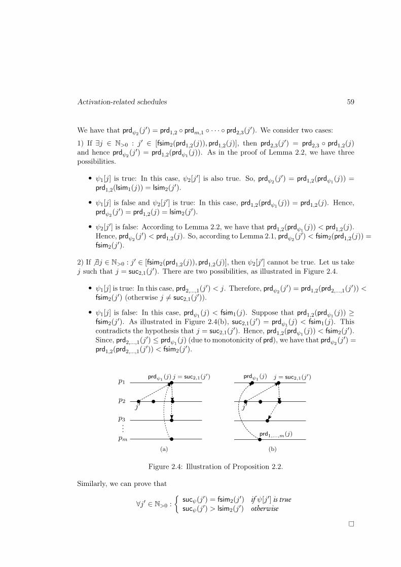
Activation-related schedules 59
We have that prdψ2(j′) = prd1,2 ◦ prdm,1 ◦ · · · ◦ prd2,3(j
′). We consider two cases:
1) If ∃j ∈ N>0 : j′ ∈ [fsim2(prd1,2(j)), prd1,2(j)], then prd2,3(j′) = prd2,3 ◦ prd1,2(j)
and hence prdψ2(j′) = prd1,2(prdψ1
(j)). As in the proof of Lemma 2.2, we have threepossibilities.
• ψ1[j] is true: In this case, ψ2[j′] is also true. So, prdψ2
(j′) = prd1,2(prdψ1(j)) =
prd1,2(lsim1(j)) = lsim2(j′).
• ψ1[j] is false and ψ2[j′] is true: In this case, prd1,2(prdψ1
(j)) = prd1,2(j). Hence,prdψ2
(j′) = prd1,2(j) = lsim2(j′).
• ψ2[j′] is false: According to Lemma 2.2, we have that prd1,2(prdψ1
(j)) < prd1,2(j).Hence, prdψ2
(j′) < prd1,2(j). So, according to Lemma 2.1, prdψ2(j′) < fsim2(prd1,2(j)) =
fsim2(j′).
2) If 6 ∃j ∈ N>0 : j′ ∈ [fsim2(prd1,2(j)), prd1,2(j)], then ψ2[j
′] cannot be true. Let us takej such that j = suc2,1(j
′). There are two possibilities, as illustrated in Figure 2.4.
• ψ1[j] is true: In this case, prd2,...,1(j′) < j. Therefore, prdψ2
(j′) = prd1,2(prd2,...,1(j′)) <
fsim2(j′) (otherwise j 6= suc2,1(j
′)).
• ψ1[j] is false: In this case, prdψ1(j) < fsim1(j). Suppose that prd1,2(prdψ1
(j)) ≥fsim2(j
′). As illustrated in Figure 2.4(b), suc2,1(j′) = prdψ1
(j) < fsim1(j). Thiscontradicts the hypothesis that j = suc2,1(j
′). Hence, prd1,2(prdψ1(j)) < fsim2(j
′).Since, prd2,...,1(j
′) ≤ prdψ1(j) (due to monotonicity of prd), we have that prdψ2
(j′) =prd1,2(prd2,...,1(j
′)) < fsim2(j′).
(a) (b)
Figure 2.4: Illustration of Proposition 2.2.
Similarly, we can prove that
∀j′ ∈ N>0 :
{
sucψ(j′) = fsim2(j
′) if ψ[j′] is truesucψ(j
′) > lsim2(j′) otherwise

60 Abstract schedules
Proposition 2.3. If Equation 2.1 holds for the closed walk ψ = p1 → p2 → · · · →pm → p1, then it holds for walk ψ′ = pm → pm−1 → · · · → p1 → pm.
Proof: Firstly, we prove that
∀j′ ∈ N>0 :
{
prdψ′(j′) = lsimm(j′) if ψ′[j′] is true
prdψ′(j′) < fsimm(j′) otherwise
There are two cases:
1) ψ′[j′] is true: As illustrated in Figure 2.5(a), if j = prdm,m−1,...,1(j′), then ψ[j] is also
true. Hence, prdψ′(j′) = prd1,m(j) = lsimm(j′).
2) ψ′[j′] is false: Let j = prdm,m−1,...,1(j′). we have that suc1,...,m(j) ≤ fsimm(j
′) andhence sucψ(j) ≤ sucm,1(j). Suppose that prdψ′(j′) ≥ fsimm(j
′) (i.e. the walk ψ′ isinconsistent). Hence, prd1,m(j) ≥ fsimm(j
′). This implies that sucm,1(j′) ≤ fsim1(j).
So, we have that sucψ(j) ≤ sucm,1(j′) ≤ fsim1(j) ≤ lsim1(j). This contradicts the
hypothesis that Equation 2.1 holds for walk ψ.Similarly, we can prove that
∀j′ ∈ N>0 :
{
sucψ′(j′) = fsimm(j′) if ψ′[j′] is true
sucψ′(j′) > lsimm(j′) otherwise
(a) (b)
Figure 2.5: Illustration of Proposition 2.3.
Composition
A cycle (or simple cycle) is a closed path; i.e. a closed walk with no repeated vertices(except the requisite repetition of the first and last vertices). For example, in Figure2.6, walks ψ = p1 → p2 → p1 and ψ′ = p2 → p3 → p4 → p5 → p2 are simple cycles;while walk ψ′′ = p1 → p2 → p3 → p4 → p5 → p2 → p1 is not a simple one. Every closedwalk can be expressed as the disjoint union of some simple cycles. For instance, ψ′′ isthe disjoint union of ψ and ψ′.

Activation-related schedules 61
Figure 2.6: Graph of activation relations.
Proposition 2.4 (Consistency of closed walks). A closed walk ψ is consistent if allsimple cycles composing ψ are consistent.
Proof:Let ψ = p1 → . . .→ p1. Suppose that pi appears more than once in ψ. Hence, ψ can
be decomposed as p1 → . . . → pi−1 → ψ′ → pi+1 → . . . → p1 such that ψ′ is the walkfrom the first occurrence of pi to the last one. Let us put ψ′′ = p1 → . . .→ pi → . . .→ p1(i.e. ψ′′ is obtained by removing the sub-walk ψ′ from ψ). We suppose that ψ′ andψ′′ are simple cycles, otherwise we have to further decompose them. We have that∀j ∈ N>0 : prdψ(j) = prdi,i+1,...,1(prdψ′(prd1,...,i−1,i(j))).
• ψ[j] is true: trivially, ψ′[prd1,...,i−1,i(j)] and ψ′′[j] are true. So, prdψ′(prd1,...,i−1,i(j)) =prd1,...,i−1,i(j). Hence, prdψ(j) = prdi,i+1,...,1(prd1,...,i−1,i(j)) = prdψ′′(j) = lsim1(j).
• ψ[j] is false: In this case, ψ′′[j] and ψ′[prd1,...,i−1,i(j)] cannot be both true. In caseψ′[prd1,...,i−1,i(j)] is true, we have that prdψ(j) = prdi,i+1,...,1(prdψ′(prd1,...,i−1,i(j))) =prdi,i+1,...,1(prd1,...,i−1,i(j)) = prdψ′′(j) < fsim1(j). In case ψ′′[j] is true, we havethat prdψ(j) = prdi,i+1,...,1(prdψ′(prd1,...,i−1,i(j))) < prdi,i+1,...,1(fsimi
(prd1,...,i−1,i(j))) = lsim1(j). The third case (i.e. when both ψ′[prd1,...,i−1,i(j)] andψ′′[j] are false) is straightforward.
Similarly, we can prove the second part of Equation 2.1.
Some simple cycles can also be expressed as the symmetric difference of some othersimple cycles. For instance, in Figure 2.6, we have that p1 → p2 → p3 → p4 → p1⊎p2 →p5 → p4 → p3 → p2 = p1 → p2 → p5 → p4 → p1.
Question 1 Let ψ,ψ′, ψ′′ be three simple cycles such that ψ = ψ′ ⊎ ψ′′. If ψ′ and ψ′′
are consistent, does this imply that ψ is also consistent?
Example 2.6 (Counterexample-Q1). In the general case, the answer to question 1
is no. The graph in Figure 2.6 is a counterexample where ψ′ = p1[(0 1 1)ω ,(1 0 0)ω ]−→
p2[(0 1)ω ,(1 0)ω ]−→ p3
[(0 1 0)ω ,(1 0 1)ω ]−→ p4[(1 0 0 1)ω ,(0 1 1 0)ω ]−→ p1 and ψ′′ = p2
[(0 1)ω ,(1 0)ω ]−→p5
[(0 0 1)ω ,(1 1 0)ω ]−→ p4[(1 0 1)ω ,(0 1 0)ω ]−→ p3
[(1 0)ω ,(0 1)ω ]−→ p2. Equation 2.1 holds for ψ′
(Figure 2.7(a)) and ψ′′ (Figure 2.7(b)) but not for ψ = ψ′ ⊎ψ′′ (Figure 2.7(c)). Indeed,prdψ(1) = 2.

62 Abstract schedules
Figure 2.7: Consistency of symmetric difference of simple cycles.
Question 2 Let ψ,ψ′, ψ′′ be three simple cycles such that ψ = ψ′ ⊎ ψ′′. If ψ isconsistent, does this imply that ψ′ and ψ′′ are also consistent?
Example 2.7 (Counterexample-Q2). In the general case, the answer to question 2 is
no. In Example 2.6, if we put p4[(1 0 1)ω ,(0 1 0)ω ]−→ p5 and p3
[(0 0 1)ω ,(1 1 0)ω ]−→ p4, thenEquation 2.1 holds for cycle ψ but not for ψ′.
Proposition 2.5 (Consistency of an abstract schedule). An abstract schedule is consis-tent if and only if every undirected cycle in the graph of activation relations is consistent.
Proof:Let Ψi,i be the set of all closed walks from pi to itself in Gr. If Equation 2.1 holds
for each walk in Ψi,i, then we will have that
∀j ∈ N>0 :
{
prdi→i(j) = lsimi(j) ∧ suci→i(j) = fsimi(j) if ∃ψ ∈ Ψi,i : ψ[j] is trueprdi→i(j) < fsimi(j) ∧ suci→i(j) > lsimi(j) otherwise
Hence, there will be no causality problems in the schedule. According to Proposition2.4 and the previous counterexamples, it is enough to check only the consistency of allthe simple cycles. According to propositions 2.2 and 2.3, it is enough to check only theconsistency of one cycle per undirected cycle in graph Gr.
Consistency of ultimately periodic schedules
Definition 2.7 (Ultimately periodic schedules). An activation relation [si,k, sk,i] is ul-timately periodic if si,k and sk,i are ultimately periodic sequences. An abstract scheduleis ultimately periodic if all its activation relations are ultimately periodic.
Hence, we can put si,k = ui,kvωi,k and sk,i = uk,iv
ωk,i such that |ui,k| = |uk,i| and
|vi,k| = |vk,i|. Example 2.2 is an ultimately periodic abstract schedule.
Proposition 2.6. A closed walk ψ = p1 → p2 → · · · → pm → p1 in an ultimatelyperiodic schedule is consistent only if
m∏
i=1
‖vi,k‖ =m∏
i=1
‖vk,i‖ (2.2)
Where k = i mod m+ 1 and ‖v‖ is the sum of elements of the finite integer sequencev.

Activation-related schedules 63
Proof:If Equation 2.1 holds for ψ, then we have that ∀j ∈ N>0 : prdψ(j) ≤ j and sucψ(j) ≥
j. Let k1 be the maximum integer for which ‖u1,2‖+k1‖v1,2‖ < fsim1(j). As illustratedin Figure 2.8, k1 is the number of instances of the positioning pattern before the instancethat contains the jth activation of p1. Since [s1,2, s2,1] is an ultimately periodic activationrelation, we have that prd1,2(j) ≥ j1 = ‖u2,1‖+ k1‖v2,1‖. Continuing the same process,k2 is the maximum integer for which ‖u2,3‖ + k2‖v2,3‖ < fsim2(j1) and so prd2,3(j1) ≥j2 = ‖u3,2‖+ k2‖v3,2‖. Hence, jm = ‖u1,m‖+ km‖v1,m‖ ≤ prdm,1(jm−1) ≤ j.
We denote by c any non important constant. We have that k1 = 1‖v1,2‖j + c, k2 =
‖v2,1‖‖v1,2‖‖v2,3‖j+c, . . . , km =
‖v2,1‖...‖vm,m−1‖‖v1,2‖...‖vm,1‖ j+c. Let us denote by
∏
ψ the product of ‖vi,k‖of all the activation relations on a walk ψ. So, prdψ(j) ≤ j implies that
∏ψ−1∏ψj + c ≤ j.
When j tends to infinity, the previous inequality has a solution only if∏
ψ−1 ≤∏
ψ.
Similarly and using the second part of Equation 2.1, we have that∏ψ−1∏ψj+c ≥ j. Thus,
∏
ψ−1 ≥∏
ψ.
positioning pattern
Figure 2.8: Illustration of Proposition 2.6.
Property 2.4. Let ψ, ψ′, and ψ′′ be three simple cycles such that ψ = ψ′ ⊎ ψ′′. IfEquation 2.8 holds for ψ′ and ψ′′, then it holds for ψ.
Proof:We prove the case where the set of edges in ψ′ that have opposites in ψ′′ forms a
contiguous path; however, the presented argument also holds for the general case. Letψ∗ = ψ′∩ψ′′ be such a contiguous path. Hence, we can put ψ′ = ψ1+ψ∗, ψ′′ = ψ2+ψ
−1∗ ,
and ψ = ψ1 + ψ2. Since Equation 2.8 holds for ψ′ and ψ′′, we have that∏
ψ1.∏
ψ∗=
∏
ψ−1
1
.∏
ψ−1∗
and∏
ψ2.∏
ψ−1∗
=∏
ψ−1
2
.∏
ψ∗. Hence,
∏
ψ1.∏
ψ2=
∏
ψ−1
1
.∏
ψ−1
2
.
2.2.3 Overflow analysis
An overflow exception occurs when an actor attempts to write to a full channel. Lete = (pi, pk, x, y) be a channel between the producer pi and the consumer pk. Theoverflow analysis ensures that the (over-approximated) number of accumulated tokensin channel e does not exceed its size δ(e) for every execution of the dataflow graph. The(over-approximated) number of accumulated tokens can be computed as follows.
• The number of produced tokens by job pi[j] is equal to x(j).

64 Abstract schedules
• The number of produced tokens before pi[j] writes any token is equal to ⊕x(j − 1)since we assume that the scheduling policy ensures, even with auto-concurrency, thatjobs of the producer write tokens in the same order of their activation. The numberof produced tokens until and including the jth job of pi is hence equal to ⊕x(j). Ifj = lsimi(j) (which is always the case if auto-concurrency is disabled), then ⊕x(j) =⊕(x⊗ si,k)(s−1
i,k (j)) = ⊕x(⊕si,k(s−1i,k (j))).
Definition 2.8 (Complete before). cbefi,k : N>0 → N is an integer function such thatpk[cbefi,k(j)] is the last job of pk which certainly reads all its needed tokens from channele before pi[j] writes any token on that channel. So, cbefi,k is a monotone function.
• The (under-approximated) number of consumed tokens before pi[j] writes any tokenon channel e is equal to ⊕y(cbefi,k(j)) since we assume that the scheduling policyensures, even with auto-concurrency, that jobs of the consumer consume tokens in thesame order of their activation. If cbefi,k(j) = lsimk(cbefi,k(j)), then ⊕y(cbefi,k(j)) =⊕(y ⊗ sk,i)(s−1
k,i (cbefi,k(j))) = ⊕y(⊕sk,i(s−1k,i (cbefi,k(j)))).
Function cbefi,k depends essentially on the scheduling policy, the physical timingparameters, and the implementation code of the firing functions. Since the abstractschedule consists of a set of timeless constraints, function cbefi,k could be only a safeapproximation that does not consider neither the timing nor the implementation code.
Example 2.8. Let us take e2 = (p1, p2, 1ω, 2ω) of the self-timed example (Figure 1.1,
p. 26). We have that cbef1,2(j) = sprd1,2(j) =⌈
j2
⌉
. Since actor p2 does not preempt
actor p1 or execute in parallel with it, function cbef1,2, as defined before, is accurate.Similarly, ∀j ≥ 2 : cbef2,3(j) = sprd2,3(j) gives the accurate values. However, since jobp2[1] executes in parallel with job p3[1], it is not safe to say that p3[1] reads the requireddata before p2[1] writes its results unless we assume that an actor reads tokens at thebeginning of firings and writes results at the end. A safe approximation for the overflowanalysis is one that over-approximates the number of accumulated tokens in channels,hence cbef2,3(1) = 0.
The (over-approximated) number of accumulated tokens on channel e when job pi[j]writes all its results can be given as
X(j) = θ(e) +⊕x(j)−⊕y(cbefi,k(j))
If the over-approximated number of accumulated tokens in the channel does notexceed the size of the channel δ(e) for all j ∈ N>0, then overflow exceptions will notoccur at run-time. Hence, the overflow analysis can be formulated as follows.
∀j ∈ N>0 : θ(e) +⊕x(j)−⊕y(cbefi,k(j)) ≤ δ(e) (2.3)
If ∀j ∈ N>0 : cbefi,k(j) = cbefi,k(lsimi(j)), then Equation 2.3 can be checked only forpoints where j = lsimi(j) since the maximum numbers of accumulated tokens happenat these points.

Activation-related schedules 65
Example 2.9. In the self-timed example and for e = (p1, p2, 1ω, 2ω), we have that
s2,1 ∈ Bω and cbef1,2(j) = cbef1,2(lsim1(j)). Thus, Equation 2.3 can be written as
∀j ∈ N>0 : θ(e) +⊕x(lsim1(j))−⊕y(cbef1,2(j)) ≤ δ(e)
We have that ∀j ∈ N>0 :
⊕x(j) = j; ⊕y(j) = 2j; cbef1,2(j) =⌈
j2
⌉
; lsim1(j) = 2⌈
j2
⌉
So,
X(j) = θ(e) + 2
⌈
j
2
⌉
− 2
⌈
j
2
⌉
= θ(e)
For θ(e) = 2, the overflow equation can be written as
∀j ∈ N>0 : δ(e) ≥ 2
The minimum safe size of channel e is hence equal to 2 (which is equal to the sizeobtained by the symbolic execution).
Boundedness
Channel e can be implemented as a bounded buffer if there are bounded constants θ(e)and δ(e) (with θ(e) ≤ δ(e)) that satisfy the overflow equation. From Equation 2.3, wehave that ⊕y(cbefi,k(j)) ≥ ⊕x(j) + θ(e) − δ(e). Since ⊕y is a monotone function, wehave that
cbefi,k(j) ≥ y−1(⊕x(j) + θ(e)− δ(e)) (2.4)
According to the second property of an activation relation (Property 2.1), there mustbe a finite number of firings of the consumer between every two firings of the producer.Hence, function cbefi,k should satisfy
∀j ∈ N>0 : cbefi,k(j)− cbefi,k(j − 1) is bounded (2.5)
Example 2.10 (SDF graphs). Let e = (p1, p2, aω, bω) be a channel in a SDF graph
where a, b ∈ N>0. We have that ⊕x(j) = aj, ⊕y(j) = bj, and y−1(j) =⌈
jb
⌉
. So,
cbef1,2(j) ≥⌈
abj + θ(e)−δ(e)
b
⌉
. For instance, if the activation relation and the scheduling
policy ensure that cbef1,2(j) = max{0,⌈
abj + θ(e)−δ(e)
b
⌉
}, then cbefi,k(j)− cbefi,k(j − 1)
is upper bounded by⌈
ab
⌉
.
2.2.4 Underflow analysis
The underflow analysis is dual to the overflow analysis. An underflow exception occurswhen an actor attempts to read from en empty channel. The underflow analysis ensuresthat the (under-approximated) number of accumulated tokens is always greater than

66 Abstract schedules
or equal to zero for every execution of the dataflow graph. The (under-approximated)number of accumulated tokens can be computed as follows.
• The number of consumed tokens by job pk[j] is equal to y(j).
• The number of consumed tokens before pk[j] reads any token is equal to ⊕y(j − 1).The number of consumed tokens until and including the jth job of pk is hence equal to⊕y(j). If j = lsimk(j), then ⊕y(j) = ⊕(y ⊗ sk,i(s−1
k,i (j)) = ⊕y(⊕sk,i(s−1k,i (j))).
• The (under-approximated) number of produced tokens before pk[j] reads any token onchannel e is equal to ⊕x(cbefk,i(j)). Function cbefk,i : N>0 → N is a monotone integerfunction such that pi[cbefk,i(j)] is the last job of pi which certainly writes all its results onchannel e before pk[j] reads any token from that channel. If cbefk,i(j) = lsimi(cbefk,i(j)),then ⊕x(cbefk,i(j)) = ⊕(x⊗ si,k)(s−1
i,k (cbefk,i(j))) = ⊕x(⊕si,k(s−1i,k (cbefk,i(j)))).
If the under-approximated number of accumulated tokens in the channel is greaterthan or equal to zero for all j ∈ N>0, then underflow exceptions will not occur at runtime. Hence, the underflow analysis can be formulated as follows.
∀j ∈ N>0 : θ(e) +⊕x(cbefk,i(j))−⊕y(j) ≥ 0 (2.6)
Example 2.11. Let us take channel e = (p2, p3, 3ω, 1ω) of the self-timed example. We
have that ∀j ≥ 2 : cbef3,2(j) = sprd3,2(j) =⌈
j−13
⌉
. Since it is not safe to say that p2[1]
writes its results before p3[1] reads any token, we must take cbef3,2(1) = 0. We havethat s2,3 ∈ Bω and cbef3,2(j) = cbef3,2(lsim3(j)). Thus, Equation 2.6 can be written as
∀j ∈ N>0 : Y (j) = θ(e) +⊕x(cbef3,2(j))−⊕y(lsim3(j)) ≥ 0
We have that
⊕x(j) = 3j; ⊕y(j) = j; lsim3(j) = 3⌈
j−13
⌉
+ 1; cbef3,2(j) =⌈
j−13
⌉
So,
Y (j) = θ(e) + 3
⌈
j − 1
3
⌉
− (3
⌈
j − 1
3
⌉
+ 1) = θ(e)− 1
The underflow equation can be written as
∀j ∈ N>0 : θ(e)− 1 ≥ 0
The minimum number of initial tokens on the channel that excludes underflow excep-tions is hence equal to 1.
Boundedness
Channel e can be implemented as a bounded buffer if there is a bounded constant θ(e)that satisfies the underflow equation. From Equation 2.6, we have that ⊕x(cbefk,i(j)) ≥⊕y(j)− θ(e). Since ⊕x is a monotone function, we have that
cbefk,i(j) ≥ x−1(⊕y(j)− θ(e)) (2.7)
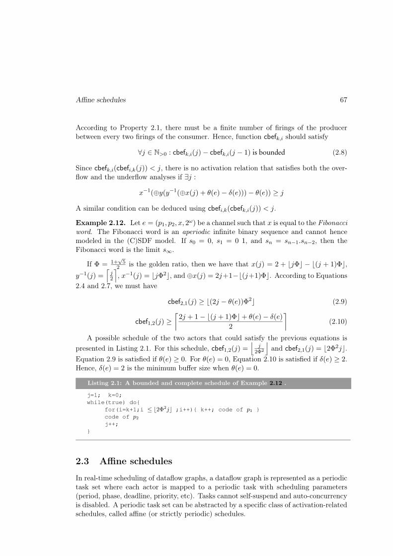
Affine schedules 67
According to Property 2.1, there must be a finite number of firings of the producerbetween every two firings of the consumer. Hence, function cbefk,i should satisfy
∀j ∈ N>0 : cbefk,i(j)− cbefk,i(j − 1) is bounded (2.8)
Since cbefk,i(cbefi,k(j)) < j, there is no activation relation that satisfies both the over-flow and the underflow analyses if ∃j :
x−1(⊕y(y−1(⊕x(j) + θ(e)− δ(e)))− θ(e)) ≥ j
A similar condition can be deduced using cbefi,k(cbefk,i(j)) < j.
Example 2.12. Let e = (p1, p2, x, 2ω) be a channel such that x is equal to the Fibonacci
word. The Fibonacci word is an aperiodic infinite binary sequence and cannot hencemodeled in the (C)SDF model. If s0 = 0, s1 = 0 1, and sn = sn−1.sn−2, then theFibonacci word is the limit s∞.
If Φ = 1+√5
2 is the golden ratio, then we have that x(j) = 2 + ⌊jΦ⌋ − ⌊(j + 1)Φ⌋,y−1(j) =
⌈
j2
⌉
, x−1(j) = ⌊jΦ2⌋, and ⊕x(j) = 2j+1−⌊(j+1)Φ⌋. According to Equations
2.4 and 2.7, we must have
cbef2,1(j) ≥ ⌊(2j − θ(e))Φ2⌋ (2.9)
cbef1,2(j) ≥⌈
2j + 1− ⌊(j + 1)Φ⌋+ θ(e)− δ(e)2
⌉
(2.10)
A possible schedule of the two actors that could satisfy the previous equations is
presented in Listing 2.1. For this schedule, cbef1,2(j) =⌊
j2Φ2
⌋
and cbef2,1(j) = ⌊2Φ2j⌋.Equation 2.9 is satisfied if θ(e) ≥ 0. For θ(e) = 0, Equation 2.10 is satisfied if δ(e) ≥ 2.Hence, δ(e) = 2 is the minimum buffer size when θ(e) = 0.
Listing 2.1: A bounded and complete schedule of Example 2.12 .
j=1; k=0;
while(true) do{
for(i=k+1;i ≤ ⌊2Φ2j⌋ ;i++){ k++; code of p1 }
code of p2j++;
}
2.3 Affine schedules
In real-time scheduling of dataflow graphs, a dataflow graph is represented as a periodictask set where each actor is mapped to a periodic task with scheduling parameters(period, phase, deadline, priority, etc). Tasks cannot self-suspend and auto-concurrencyis disabled. A periodic task set can be abstracted by a specific class of activation-relatedschedules, called affine (or strictly periodic) schedules.

68 Abstract schedules
2.3.1 Affine relations
Affine transformations of abstract clocks were introduced in [168] (Definition 1.4, p.22). In this section, we will approach them differently using ultimately periodic binarysequences. Activation clocks pi and pk are (n, ϕ, d)-affine-related, with n, d ∈ N>0 andϕ ∈ Z, if in case ϕ is positive (resp. negative), clock pi is obtained by counting eachnth instant on a referential abstract clock c starting from the first (resp. (−ϕ + 1)th)instant; while clock pk is obtained by counting each dth instant on c starting from the(ϕ+ 1)th (resp. first) instant. Hence, we have ∀j ∈ N>0 (j denotes the jth tag in c)
pi(j) =
{
1 if ∃t ∈ N : j = nt+max{1,−ϕ+ 1}0 otherwise
and
pk(j) =
{
1 if ∃t ∈ N : j = nt+max{1, ϕ+ 1}0 otherwise
Figure 2.9 represents a (3,−4, 5)-affine relation.
Figure 2.9: A (3,−4, 5)−affine relation.
Property 2.5. pi and pk are ultimately periodic binary sequences.
Proof : We have that ∀j ∈ N>0 : pi(j+nd
gcd{n,d}) = pi(j) and pk(j+ ndgcd{n,d}) = pk(j).
Therefore, there is a positioning pattern that repeats infinitely, as depicted in Fig-ure 2.9. It consists of d
gcd{n,d} activations of pi and ngcd{n,d} activations of pk. Thus,
parameters n and d of an affine relation encode the ratio between activation rates ofactors. For instance, a (1, ϕ, 2)-affine relation means that pi is twice as fast as actor pk.Parameter ϕ encodes the difference between the first start times of the two actors.
Property 2.6. If pi and pk are (n, ϕ, d)-affine-related, then pk and pi are (d,−ϕ, n)-affine-related.
In the sequel, ϕ is supposed to be positive (unless it is stated otherwise). Whenϕ is negative, it is sufficient to reverse the affine relation and then obtain the desiredproperty.
Property 2.7. An affine relation contains synchronous activations if and only ifgcd{n, d} divides ϕ.
Proof : If pi[j] = pk[j′], then pi(nj−n+1) = pk(dj
′−d+ϕ+1) = 1 and nj−dj′ = ϕ+n−d.We have two cases:(i) gcd{n, d}|ϕ: the diophantine equation n
gcd{n,d}j − dgcd{n,d}j
′ = ϕ+n−dgcd{n,d} have an in-
finite number of solutions. If the first synchronization occurs at (j1, j′1), then the lth

Affine schedules 69
synchronization occurs at (j1 +(l−1)d
gcd{n,d} , j′1 +
(l−1)ngcd{n,d}). Hence, there is exactly one syn-
chronization per positioning pattern instance.(ii) gcd{n, d} 6 |ϕ: Equation nj − dj′ = ϕ+ n− d has no solution.
Since we are not interested in tags where both clocks are absent, we define an affinerelation as an ultimately periodic activation relation [si,k = uiv
ωi , sk,i = ukv
ωk ]. We have
that (assuming that ϕ is positive)
• |ui| = |uk| =⌈
ϕn
⌉
; ∀j ≤ |ui| : ui(j) = 1 and uk(j) = 0.
• According to Property 2.7,
|vi| = |vk| =n+ d
gcd{n, d} −{
1 if gcd{n, d}|ϕ0 otherwise
• ‖vi‖ = dgcd{n,d} and ‖vk‖ = n
gcd{n,d} .
Example 2.13. For the affine relation in Figure 2.9, we have that si,k = 0(1 0 1 1 1 0 1)ω
and sk,i = 1(0 1 0 1 0 1 0)ω.
We have also that sprdi,k(j) = max{0,⌈
n(j−1)−ϕd
⌉
}, prdi,k(j) = max{0,⌊
n(j−1)−ϕd
⌋
+
1}, ssuci,k(j) = prdi,k(j) + 1, and suci,k(j) = sprdi,k(j) + 1. To obtain sprdk,i, prdk,i,ssuck,i, and suck,i, we need just to reverse the affine relation. Let ξ(j) be the number ofsynchronizations until and including pi[j], and pi[j1] be the first job of pi synchronizedwith a job of pk. So, we have that s−1
i,k (j) = j + prdi,k(j)− ξ(j) and
ξ(j) =
{
0 if gcd{n, d} 6 |ϕmax{0,
⌊
(j−j1) gcd{n,d}d
⌋
+ 1} otherwise
Canonical form
An infinite number of affine transformations can result in the same activation relation.For instance, (n, ϕ, d) and (cn, cϕ, cd) (where c is an integer constant) result in the sameactivation relation. A canonical form is therefore proposed in [167]. Let g = gcd{n, d}.So,
(i) g|ϕ: (n, ϕ, d) ≡ (ng, ϕg, dg).
(ii) g 6 |ϕ: (n, ϕ, d) ≡ (2ng, 2
[
ϕg
]
+ 1, 2dg).
The first case is obvious; the second case needs a proof. We present here a muchsimpler proof than the one presented in [167].
Proof: Let (n, ϕ, d) ≡ (n′, ϕ′, d′) with n′ = mng
and d′ = mdg
. We need to find theminimum integers m (m ≥ 1) and ϕ′ such that both affine transformations result in thesame activation relation; hence in the same sprdi,k and ssuci,k.

70 Abstract schedules
sprdi,k(j) =⌈
n′(j−1)−ϕ′
d′
⌉
=⌈
n(j−1)−ϕd
+ ϕd− gϕ′
md
⌉
. The two affine transformations
are equivalent only if⌈
n(j−1)−ϕd
⌉
=⌈
n(j−1)−ϕd
+ ϕd− gϕ′
md
⌉
. Let d0 ≥ 1 and d1 ≥ 1 be
the minimum integers such that d|n(j−1)−ϕ−d0 and d|n(j−1)−ϕ+d1, respectively.Note that d0 and d1 are greater or equal to 1 because the affine relation does not containany synchronous activations (since g 6 |ϕ). Hence, we must have −d0 < ϕ − g
mϕ′ ≤ d1.
Following the same process with ssuci,k, we should have the constraint −d0 ≤ ϕ− gmϕ′ <
d1. Therefore, ϕ−d1g
< ϕ′
m< ϕ+d0
g. So, we must have
ϕ−minjd1
g< ϕ′
m<
ϕ+minjd0
g. Since
minjd0 +min
jd1 = g, bounds
ϕ−minjd1
gand
ϕ+minjd0
gare two successive integers. Hence,
the minimum value of m is 2 and the minimum value of ϕ′ is 2[
ϕg
]
+ 1.
2.3.2 Consistency
An affine schedule consists of a set of affine relations. Let Gr be the graph of affinerelations.
Proposition 2.7. A closed walk p1(n1,ϕ1,d1)−→ p2 → · · · → pm
(nm,ϕm,dm)−→ p1 is consistentonly if
m∏
i=1
ni =m∏
i=1
di (2.11)
Proof: Since an affine schedule is also an ultimately periodic schedule, a closed walk in
Gr is consistent only if Proposition 2.8 is satisfied; i.e.m∏
i=1‖vi,k‖ =
m∏
i=1‖vk,i‖ with k = i
mod m+ 1. But, ‖vi,k‖ = digcd{ni,di} and ‖vk,i‖ = ni
gcd{ni,di} .
Proposition 2.8. A closed walk p1(n1,ϕ1,d1)−→ p2 → · · · → pm
(nm,ϕm,dm)−→ p1 is consistentif Equation 2.11 is satisfied and
m∑
i=1
(
i−1∏
j=1
dj)(
m∏
j=i+1
nj)ϕi = 0 (2.12)
Proof: Let us put Xm =m∏
i=1ni, Ym =
m∏
i=1di, and Zm =
m∑
i=1(i−1∏
j=1dj)(
m∏
j=i+1nj)ϕi. We have
two cases.(i) ψ[j] is true: In this case, prd1,2(j) =
X1j−Z1
Y1− X1
Y1+1, prd1,2,3(j) =
X2j−Z2
Y2− X2
Y2+1,
etc. Since Xm = Ym, we have that prdψ(j) = j − ZmYm
. According to Proposition 2.1,prdψ(j) = j; hence Zm = 0. Similar process can be done for sucψ.
(ii) ψ[j] is false: Since prdψ(j) < j − ZmYm
< sucψ(j), condition Zm = 0 is a sufficientcondition for consistency.

Affine schedules 71
Example 2.14. Proposition 2.8 is a sufficient but non-necessary condition for consis-
tency of a cycle. If p1(3,5,5)−→ p2
(4,−8,3)−→ p3(n3,ϕ3,d3)−→ p1, then according to Equations 2.11
and 2.12 we have that 4n3 = 5d3 and 4n3 = 3ϕ3. So, (n3, ϕ3, d3) ≡ (15k, 20k, 12k) fork ≥ 1. Since gcd{15k, 12k} 6 |20k, the canonical form is (10, 13, 8). However, Equation2.12 does not hold when (n3, ϕ3, d3) = (10, 13, 8). The affine schedule is also consistentwhen (n3, ϕ3, d3) = (10, 11, 8), as illustrated in Figure 2.10. Equation 2.12 does notalso hold in this case. All the affine transformations that are equivalent with (10, 11, 8)can be written as (5k, ϕ, 4k) with 5k < ϕ < 6k. All these affine transformations cannotsatisfy Equation 2.12.
Figure 2.10: A consistent affine schedule.
Property 2.8. Equation 2.12 is a necessary condition if the following equation systemadmits a solution.
Γ~x = ~ϕ (2.13)
where ~ϕ(i) = ϕi, and for every affine relation pi(ni,ϕi,di)−→ pk with k = (i mod m) + 1,
we have that Γi,i = ni and Γi,k = −di.
Proof: Firstly, if Equation 2.13 admits a solution, then it admits an infinite number ofsolutions since det(Γ) = Xm − Ym = 0. If ~x is a solution, then ∀i = 1,m : ni~x(i) −di~x(k) = ϕi such that k = (i mod m) + 1. Hence, prdi,k(~x(i) + 1) = suci,k(~x(i) + 1) =~x(k) + 1. So, pi[~x(i) + 1] = pk[~x(k) + 1]. Thus, ψ[~x(1) + 1] is true. According to theproof of Proposition 2.8, Zm must be equal to zero.
In real-time scheduling of dataflow graphs, we need to have a global referentialclock. Therefore, Proposition 2.8 must hold for every simple cycle in the graph of affinerelations.
Proposition 2.9. Let ψ, ψ′, ψ′′ be three simple cycles such that ψ = ψ′ ⊎ ψ′′ andψ′ ∪ ψ′′ forms a continuous path. If Proposition 2.8 holds for ψ′ and ψ′′, then it holdsfor ψ.
Proof: According to Property 2.4 and since an affine schedule is also an ultimatelyperiodic schedule, we have that Equation 2.11 holds for cycle ψ. Since the set of edgesin ψ′ that have opposites in ψ′′ forms a contiguous path, we can put ψ′ = ψ1+ψ∗, ψ′′ =ψ2 +ψ−1
∗ , and ψ = ψ1 +ψ2. To ease the notations, we illustrate the proof for Equation

72 Abstract schedules
2.12 on an example. Let ψ∗ = p2(n,ϕ,d)−→ p3
(n′,ϕ′,d′)−→ p4, ψ1 = p4(n4,ϕ4,d4)−→ p1
(n1,ϕ1,d1)−→ p2,
and ψ2 = p2(n2,ϕ2,d2)−→ p5
(n5,ϕ5,d5)−→ p4.So, we have that Zψ′ = n1ϕ4nn
′ + d4ϕ1nn′ + d4d1ϕn
′ + d4d1ϕ′d = 0 and Zψ′′ =
n5ϕ2d′d+d2ϕ5d
′d−d2d5ϕ′d−d2d5ϕn′ = 0. We then eliminate common terms: d2d5Zψ′+
d4d1Zψ′′ = n5d4d1ϕ2dd′ + d2d4d1ϕ5dd
′ + n1d2d5ϕ4nn′ + d4d2d5ϕ1nn
′ = 0. Using nn′
dd′=
d4d1n4n1
(Equation 2.11 on cycle ψ′), we obtaind2d5Zψ′+d4d1Zψ′′
dd′= Zψ = 0.
Generally, if Xψ is the product of parameters n of affine relations on walk ψ and Yψis the product of parameters d of affine relations on walk ψ, then
Yψ1Zψ′′ + Yψ2
Zψ′ = Yψ∗Zψ
Proposition 2.10 (Consistency of affine schedules). An affine schedule is consistent ifEquations 2.11 and 2.12 hold for every fundamental cycle in the graph of affine relations.
A fundamental cycle is an undirected cycle that is obtained when adding an edgeto the spanning tree (or the spanning forest if Gr is not connected) of the graph ofaffine relations. There is a one-to-one correspondence between fundamental cycles andedges not in the spanning tree. if Gr = (P,R) is connected, then there are |R| −N + 1fundamental cycles. Fundamental cycles form a basis for the cycle space; i.e. anyundirected cycle in the graph can be expressed as the symmetric difference of somefundamental cycles. According to Proposition 2.9, we need to check consistency of onlycycles in a cycle basis. Finding a cycle basis is a well-known problem in graph theory[110] that can be solved in polynomial time. Finding the minimum cycle basis (i.e. thetotal number of edges in the cycle basis is minimum) could be interesting to reduce thelength of constraints (i.e. Equation 2.12).
2.3.3 Fixed-priority schedules
In FP scheduling, each actor pi has a constant priority sequence ωi = (wi)ω. We assume
that each actor can have a distinguished priority. At each instant of the execution, a FPscheduler chooses the task with the highest priority among all activated tasks to executeon a given processor. In case of partitioned scheduling, each actor is permanentlyallocated to processor number νi; while in global scheduling, a job can migrate from oneprocessor to another. We will show in the next chapter how to compute the schedulingparameters wi and νi of each actor. In this section, we present how to compute aFP abstract schedule using Linear Integer Programming (ILP). The abstract scheduleconsists of an affine relation between every two adjacent (i.e. communicating) actors.The abstract schedule should exclude overflow and underflow exceptions.
A Overflow analysis
Let e = (pi, pk, x, y) be a channel between the (n, ϕ, d)-affine-related actors pi and pk.The affine relation is under the canonical form. Firstly, we need to compute function

Affine schedules 73
cbefi,k that corresponds to a FP scheduling policy without considering the physicaltiming. Figures 2.11 illustrates for all possible cases which last job of pk certainly readsall its needed tokens from channel e before pi[j] writes any token on that channel. Letj′ = prdi,k(j) and j′′ = cbefi,k(j).
(i) Partitioned scheduling:
a. wi < wk, νi = νk, and pi[j] 6= pk[j′]: When job pi[j] is released, it may be possible
that pk[j′] has not yet finished reading from channel e. In this case, pi[j] preemptspk[j
′] because pi has the highest priority and both jobs are allocated to the sameprocessor. Thus, we are only certain that pk[j′ − 1] has already finished. A safeapproximation is hence to put cbefi,k(j) = prdi,k(j)− 1.
b. wi < wk, νi = νk, and pi[j] = pk[j′]: jobs pi[j] and pk[j
′] are released simultane-ously to execute on the same processor. Thus, pi[j] will execute first because ithas the highest priority. Hence, cbefi,k(j) = prdi,k(j)− 1.
c. wi < wk, νi 6= νk, and pi[j] 6= pk[j′]: As in case (a), cbefi,k(j) = prdi,k(j)− 1.
d. wi < wk, νi 6= νk, and pi[j] = pk[j′]: As in case (b), cbefi,k(j) = prdi,k(j)− 1.
e. wi > wk, νi = νk, and pi[j] 6= pk[j′]: Since pk[j′] has a higher priority than pi[j]
and pk[j′] is released first, we are certain that pk[j′] ends before pi[j] starts writingany token. Hence, cbefi,k(j) = prdi,k(j).
f. wi > wk, νi = νk, and pi[j] = pk[j′]: As in the previous case, cbefi,k(j) = prdi,k(j).
g. wi > wk, νi 6= νk, and pi[j] 6= pk[j′]: Though pk[j
′] is released before pi[j] andpk[j
′] has the highest priority, we are not certain that pk[j′] completes readingfrom channel e before pi[j] starts writing. Indeed, pi[j] and pk[j
′] can execute inparallel with each other because they are allocated to different processors. A safeapproximation is hence cbefi,k(j) = prdi,k(j)− 1.
h. wi > wk, νi 6= νk, and pi[j] = pk[j′]: pi[j] can execute in parallel with pk[j
′].Thus, cbefi,k(j) = prdi,k(j)− 1.
Figure 2.11: Function cbefi,k: partitioned fixed-priority scheduling.

74 Abstract schedules
To sum up, it is certain that the last job of pk released before or simultaneously withpi[j], completes reading from channel e before pi[j] starts writing on e only if pk has ahigher priority than pi and both actors are allocated to the same processor. Therefore,
cbefi,k(j) =
{
max{0, prdi,k(j)− 1} if wi < wk ∨ νi 6= νkprdi,k(j) otherwise
(ii) Global scheduling: It is possible that there are enough resources to execute pi[j] andpk[j
′] in parallel with each other. Hence, a safe approximation is to take cbefi,k(j) =max{0, prdi,k(j)− 1}.
Channel e is overflow-free if Equation 2.3 is satisfied. Unfortunately, that equationis not a linear constraint. Similarly to real-time calculus, we approximate the numberof accumulated tokens by upper and lower bound curves. However, the curves are time-independent. If ⊕xu is the upper bound curve of ⊕x, ⊕yl is the lower bound curve of⊕y, and cbefli,k is the lower bound curve of cbefi,k, then the over-approximated numberof accumulated tokens is given as
Xu(j) = θ(e) +⊕xu(j)−⊕yl(cbefli,k(j))
In order to compute cbefli,k, we need to compute the lower bound of⌊
n(j−1)−ϕd
⌋
which could be taken as the linear bound ndj − ϕ+n+d−1
d. Since an actor produces
or consumes a finite number of tokens at each firing, the cumulative function of a ratefunction x can be linearly bounded. Suppose that we have ∀j ∈ N : ⊕xl(j) = axj+λ
lx ≤
⊕x(j) ≤ ⊕xu(j) = axj+λux with ax ∈ Q>0. If cbefi,k(j) = prdi,k(j)− 1, then we obtain
Xu(j) = (ax − ayn
d)j + θ(e) + λux − λly + ay
ϕ+ n+ d− 1
d
The number of accumulated tokens is bounded only if ax − ay nd = 0. Thus, theboundedness criterion is
n
d=axay
(2.14)
Since n and d can be deduced from the boundedness criterion, the overflow equationcan be written as a simple linear constraint
θ(e)− δ(e) + aydϕ ≤ λly − λux − ay
n+ d− 1
d(2.15)
where ϕ is the free integer variable. The size of the channel and the number of its initialtokens can be either predefined or free variables. If cbefi,k(j) = prdi,k(j), we obtain thefollowing linear constraint.
θ(e)− δ(e) + aydϕ ≤ λly − λux − ay
n− 1
d(2.16)

Affine schedules 75
B Underflow analysis
The underflow analysis is dual to the overflow analysis. We first need to computefunction cbefk,i that corresponds to a FP scheduling policy without considering thephysical timing. Figure 2.12 illustrates for some possible cases which last job of picertainly writes all its results on channel e before pk[j] reads any token from thatchannel.
Figure 2.12: Function cbefk,i: partitioned fixed-priority scheduling.
In partitioned scheduling, cbefk,i(j) = prdk,i(j) if wi < wk and νi = νk (cases (a)and (b)); and cbefk,i(j) = prdk,i(j) − 1 otherwise. In global scheduling, cbefk,i(j) =prdk,i(j)− 1 (cases (c) and (d)). The number of accumulated token in channel e can beunder-approximated as
Y l(j) = θ(e) +⊕xl(cbeflk,i(j))−⊕yu(j)
If cbefk,i(j) = prdk,i(j) − 1, then cbefk,i(j) can be linearly lower bounded by dnj +
ϕ−n−d+1n
. Hence,
Y l(j) = (axd
n− ay)j + θ(e) + λlx − λuy + ax
ϕ− n− d+ 1
n
But, ax dn − ay = 0 (the boundedness criterion). Therefore, the underflow equation canbe written as the following linear constraint.
θ(e) +aydϕ ≥ λuy − λlx + ay
n+ d− 1
d(2.17)
When cbefk,i(j) = prdk,i(j), the linear underflow constraint is given as.
θ(e) +aydϕ ≥ λuy − λlx + ay
d− 1
d(2.18)
If we combine the overflow equation with the underflow equation, then we cancompute an approximate size of the channel as illustrated in Table 2.1 where λ =(λuy +λ
ux)− (λly+λ
lx). These approximate sizes are useful when computing the schedul-
ing parameters. For instance, the gain in storage space that comes from switchingthe priorities of two actors allocated to the same processor is approximatively equal toay|d−nn |.

76 Abstract schedules
νi = νk νi 6= νkwi < wk λ+ ay
n+2d−2d
λ+ ay2n+2d−2
d
wi > wk λ+ ay2n+d−2
dλ+ ay
2n+2d−2d
Table 2.1: Approximate buffer sizes in fixed-priority scheduling.
C Algorithm
If the graph of affine relations is acyclic, then every affine relation can be computedindependently of the other relations. Parameters n and d can be deduced from theboundedness criterion; while parameter ϕ is computed (using an enumerative solutionor the approximate overflow and underflow equations) so that the total sum of sizes ofthe channels between pi and pk is minimized.
When the graph of affine relations is cyclic, consistency of the schedule must beconsidered. Firstly, we use Equation 2.14 to deduce parameters n and d of every affinerelation, then Equation 2.11 is applied on every fundamental cycle in Gr. To computethe parameters ϕ, we construct an integer linear program by applying overflow andunderflow linear constraints on channels; and Equation 2.12 on fundamental cycles.The objective function of the linear program is to minimize the buffering requirements.From the overflow and underflow equations, we can notice that lim
|ϕ|→+∞δ(e)|ϕ| =
ayd
. This
indicates that the best values of ϕ are in the neighborhood of 0.The number of initial tokens in channels could be insufficient and an underflow-free
affine schedule does not hence exist. It is also possible to not find an underflow-freeschedule because of the conservative approximation made in the overflow and underflowanalyses. One option is to not specify the numbers of initial tokens and so let thescheduling tool compute the appropriate values. Sizes obtained by the solution of thelinear program are a safe approximation of the actual sizes. Therefore, they may berecomputed after obtaining the affine relations. The minimum number of initial tokensis given by θ(e) = |min{0,min
j{⊕x(cbefk,i(j))−⊕y(j)}}| and the minimum size of the
channel is given by δ(e) = maxj{θ(e) +⊕x(j)−⊕y(cbefi,k(j))}.
As shown in the previous chapter, retiming techniques can be used to redistribute theinitial tokens in order to improve the throughput. If the production and consumptionrates are constant, then retiming can be easily expressed as linear constraints. If e =(pi, pk, a
ω, bω) and ~z is the retiming vector, then we have to add the linear constraintθ(e) = θ′(e) + a~z(i)− b~z(k) where θ′(e) is the user-provided number of initial tokens inthe channel.
2.3.4 EDF schedules
In EDF scheduling, the job with the earliest absolute deadline has the highest priority.If two jobs pi[j] and pk[j
′] have the same absolute deadlines, then the job which isreleased first gets the highest priority. However, if the two jobs are synchronous, thenwe use the actors’ ID to break the tie. In this section, we show how to compute the

Affine schedules 77
affine schedule when the dataflow graph is modeled as an implicit periodic task set. Wealso show the impact of the totally ordered communication strategy on the bufferingrequirements.
A Implicit task model
Each job p[j] has an absolute deadline that has the same tag as the next release p[j+1].Let e = (pi, pk, x, y) be a channel between two (n, ϕ, d)-affine-related actors. Regardingthe overflow analysis, we need to compute function cbefi,k that corresponds to the EDFscheduling of implicit task sets. Figures 2.13 illustrates for some possible cases whichlast job of pk certainly reads all its needed tokens from channel e before pi[j] writes anytoken on that channel. Let j′ = prdi,k(j) and j′′ = cbefi,k(j).
(i) Partitioned scheduling (νi = νk):
a,b. pi[j] 6= pk[j′] and pk[j′ + 1] ≤ pi[j + 1]: According to the EDF policy, pk[j′] has a
higher priority than pi[j]. Since pk[j′] is released before pi[j] and the two actorsare allocated to the same processor, pk[j′] will end before pi[j] starts executing.Hence, cbefi,k(j) = prdi,k(j).
c. pi[j] 6= pk[j′] and pi[j + 1] < pk[j
′ + 1]: job pk[j′] is released first; but it can be
preempted by pi[j] since this latter has the highest priority. Hence, it is safe totake cbefi,k(j) = prdi,k(j)− 1.
d. pi[j] = pk[j′] and pk[j
′ + 1] < pi[j + 1]: pk[j′] has a higher priority than pi[j].Therefore, cbefi,k(j) = prdi,k(j).
e. pi[j] = pk[j′] and pi[j + 1] = pk[j
′ + 1]: To break the tie, we need to look atthe actors’ ID. If ID(pk) < ID(pi), then cbefi,k(j) = prdi,k(j); else cbefi,k(j) =prdi,k(j)− 1.
f. pi[j] = pk[j′] and pi[j + 1] < pk[j
′ + 1]: job pi[j] has a higher priority than pk[j′].Hence, cbefi,k(j) = prdi,k(j)− 1.
(a) (b) (c)
(d) (e) (f)
Figure 2.13: Function cbefi,k: partitioned EDF scheduling, νi = νk.
There are only three cases in which cbefi,k(j) = prdi,k(j)− 1 (cases (c), (e), and (f))and which are possible only if d−n
gcd{n,d} ≥ 2 or if n = d ∧ ID(pi) < ID(pk).

78 Abstract schedules
(ii) Partitioned scheduling (νi 6= νk) or global scheduling: In these cases, priorities do notguarantee any precedences between jobs as shown in the FP scheduling. For instance,in Figure 2.13, case (a), jobs pk[j′] and pi[j] can execute in parallel with each other. So,for all possible cases, we have that cbefi,k(j) = prdi,k(j)− 1.
The underflow analysis is dual to the overflow analysis. For instance, if pk[j] = pi[j′],
νi = νk, and pk[j + 1] < pi[j′ + 1], then cbefk,i(j) = prdk,i(j) − 1. The overflow and
underflow linear equations can be computed as in the FP scheduling. Similarly, wecan deduce the approximate gain that comes from allocating two actors to the sameprocessor.
B Totally ordered communication
Consider the case when the producer pi and the consumer pk are all allocated to thesame processor. As illustrated in Figure 2.13 case (c), worst-case overflow and underflowscenarios are considered when there is a potential preemption. Besides reducing thecontext switching overhead, eliminating preemptions will definitely result in a moreaccurate analysis and hence less buffering requirements.
The totally ordered communication strategy between pi and pk is defined as follows.If pi[j] is released before pk[j
′], then pi[j] executes entirely before pk[j′]. Similarly,
if pk[j′] is released before pi[j], then pk[j′] executes entirely before pi[j]. In the next
chapter, we will describe how to implement this communication strategy without usinglock-based synchronization mechanisms.
For the overflow analysis, we will have cbefi,k(j) = prdi,k(j) in cases (a,b,c,d) ofFigure 2.13 and cbefi,k(j) = prdi,k(j) − 1 in case (f). We need to look at actors’ ID tobreak the tie in case (e). The difference between the implicit task model and the totallyordered communication strategy lies in case (c); i.e. when d−n
gcd{n,d} ≥ 2. In this case,the linear overflow and underflow equations are
λuy − λlx + ayd− 1
d≤ θ(e) + ay
dϕ ≤ δ(e) + λly − λux − ay
n
d
Compared to the implicit task model, the approximate gain on buffering require-ments is hence equal to ay
d−1d
. Similarly, if n−dgcd{n,d} ≥ 2, then the consumer may
preempt the producer. The approximate gain that comes from the totally orderedcommunication will be equal to ax n−1
n.
One important question about the totally ordered communication strategy is whetherimposing scheduling precedences may create deadlocked cycles. The answer is no be-cause we enforce a scheduling precedence from pi to pk only when n−d
gcd{n,d} ≥ 2. Thisproperty cannot be satisfied by all relations on a cycle.
2.4 Specific cases
In this section, we refine our technique for ultimately cyclo-static dataflow graphs. Wealso extend the approach to consider multichannels, shared storage space, synchronoussemantics, etc.

Specific cases 79
2.4.1 Ultimately cyclo-static dataflow graphs
Definition 2.9 (UCSDF graph). An ultimately cyclo-static dataflow (UCSDF) graphis a static dataflow graph where production and consumption rates are ultimately peri-odic.
Figure 2.14: An ultimately cyclo-static dataflow graph.
Figure 2.14 represents an UCSDF graph. It is not evident how to transform anUCSDF graph to an equivalent SDF graph without refactoring the code. Let us consider avery simple UCSDF graph G = ({p1, p2}, e = (p1, p2, x = u1v
ω1 , y = u2v
ω2 )). This graph
can be modeled as a (C)SDF graph only if there are two finite integers j1 ≥ |u1| andj2 ≥ |u2| such that θ(e) + ⊕x(j1) − ⊕y(j2) = 0. For example, if x = 3 0(2 1)ω, y =3(2 0 1)ω, and θ(e) = 2, then j1 = 2 and j2 = 2. This way the graph can be partitionedinto two disjoint (C)SDF graphs: a deadlocked graph and a live one, as illustrated inFigure 2.15. Note that actor p1[1] will fire only once (and hence corresponds to the firstjob of actor p1) because of the non-consistent self loop.
Figure 2.15: (a) An UCSDF graph and (b) its equivalent CSDF graph.
There are some problems in this transformation method: (1) The resulted graphis non-consistent, which hinders the use of analysis tools for (C)SDF graphs. (2) Wecannot disable auto-concurrency because this requires to add edges from the deadlockedsubgraph into the live one and hence turns this latter into a deadlocked graph. (3) TheUCSDF graph in Figure 2.14 cannot be transformed because it is not possible to findthree finite integers j1 ≥ 1, j2 ≥ 2, and j3 ≥ 1 that bring the marking to [0 0 0]T.
If Γ denotes the reachability graph in Figure 1.2 (p. 27), then the reachability graph

80 Abstract schedules
of the UCSDF example (Figure 2.14) is
000
p2−→
003
p3−→
101
p3−→
300
p1−→
040
p2−→ Γ
Therefore, there are an infinite number of live and bounded static schedules for theUCSDF example. All these schedules start with the prefix p2 p3 p3 p1 p2. Unlikein reachability graphs of (C)SDF graphs, it is possible that the initial marking of anUCSDF graph is not a home marking (i.e. there is no firing sequence that brings thegraph to its initial state).
Affine scheduling
Let x = uvω be an ultimately periodic rate function. So, ⊕x is a function that increasesby ‖v‖ every |v| steps. Therefore, the cumulative function can be linearly boundedby axj + λlx ≤ ⊕x ≤ axj + λux where ax = ‖v‖
|v| , λlx = min
0≤j≤|u|+|v|{⊕x(j) − ‖v‖
|v| j},
and λux = max0≤j≤|u|+|v|
{⊕x(j) − ‖v‖|v| j}. Figure 2.16 illustrates the linear bounds for x =
2 0 1(2 1 0 2)ω.
Figure 2.16: Linear bounds of ultimately periodic rates.
If e = (pi, pk, x = u1vω1 , y = u2v
ω2 ) is a channel between pi and pk, then the affine
relation between the two actors must satisfy the boundedness criterion
n
d=axay
=‖v1‖|v1|
|v2|‖v2‖
Question: Is there an affine schedule among all the possible static schedules of theUCSDF example?
Firstly, it is worth recalling that the positioning pattern in an affine relation alwaysconsists of d
gcd{n,d} activations of pi and ngcd{n,d} activations of pk whatever the parameter
ϕ. Using the boundedness criterion, we may have p1(2,ϕ1,4)−→ p2
(6,ϕ2,2)−→ p3(4,ϕ3,6)−→ p1. Let
us consider the static schedule p2 p3 p3 p1 p2(p2 p3 p3 p1 p3 p1)ω. By projecting this

Specific cases 81
schedule on each pair of the actors, we obtain the activation relations in Figure 2.17.Assuming an EDF scheduling policy with a totally ordered communication strategy ona single processor, we have to find the affine relations that give the same order of firingsas in the static schedule. So, the activation relation between p1 and p3 corresponds to
the affine relation p1(6,−7,4)−→ p3. However, there is no affine relation (by enumerating
values of ϕ1) that can give the same order of firings as in Figure 2.17.(a) because of theprefix. Therefore and for the same reason, there is no underflow-free affine schedule forthe chosen scheduling policy. This is why it is better to let the scheduling tool computethe appropriate numbers of initial tokens.
Figure 2.17: Activation relations of the schedule p2 p3 p3 p1 p2(p2 p3 p3 p1 p3 p1)ω.
2.4.2 Multichannels
Let e = (pi, pk, pl, x, y, z) be a channel that relates two producers pi and pk (allocatedto the same processor) to one consumer pl. We impose a totally ordered communicationstrategy between producers; i.e. a job of a producer cannot preempt a job of the otherproducer. This way, if the affine relation between pi and pk is predefined or if all thepossible values of the affine relation result in the same order of firings of the producers,then the producers write tokens on channel e in a deterministic way. We have hence adeterministic merge operator.
Like with simple channels, the number of accumulated tokens must be always smallerthan or equal to the size of the channel and greater than or equal to zero. The overflowanalysis can be written as
∀j ∈ N>0 : θ(e) +⊕x(j) +⊕y(cbefi,k(j))−⊕z(cbefi,l(j)) ≤ δ(e)∀j ∈ N>0 : θ(e) +⊕x(cbefk,i(j)) +⊕y(j)−⊕z(cbefk,l(j)) ≤ δ(e)
The number of accumulated tokens can be linearly over-approximated by considering⊕xu, ⊕yu, ⊕zl, cbefui,k, cbefuk,i, cbefli,l, and cbeflk,l. Dually, the underflow analysis canbe written as
∀j ∈ N>0 : θ(e) +⊕x(cbefl,i(j)) +⊕y(cbefl,k(j))−⊕z(j) ≥ 0
The number of accumulated tokens can be linearly under-approximated by considering
⊕xl, ⊕yl, ⊕zu, cbefll,i, and cbefll,k. If pi(n1,ϕ1,d1)−→ pk
(n2,ϕ2,d2)−→ pl(n3,ϕ3,d3)−→ pi, then the
boundedness criterion will be
az = axn3d3
+ ayd2n2
Similar analysis can be performed on channels with two consumers and one producer.This construct represents the deterministic select operator.
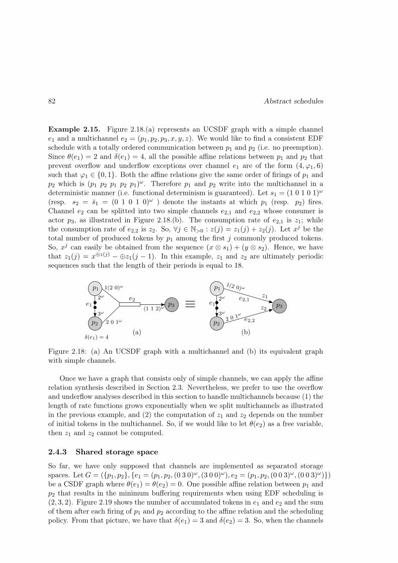
82 Abstract schedules
Example 2.15. Figure 2.18.(a) represents an UCSDF graph with a simple channele1 and a multichannel e2 = (p1, p2, p3, x, y, z). We would like to find a consistent EDFschedule with a totally ordered communication between p1 and p2 (i.e. no preemption).Since θ(e1) = 2 and δ(e1) = 4, all the possible affine relations between p1 and p2 thatprevent overflow and underflow exceptions over channel e1 are of the form (4, ϕ1, 6)such that ϕ1 ∈ {0, 1}. Both the affine relations give the same order of firings of p1 andp2 which is (p1 p2 p1 p2 p1)
ω. Therefore p1 and p2 write into the multichannel in adeterministic manner (i.e. functional determinism is guaranteed). Let s1 = (1 0 1 0 1)ω
(resp. s2 = s1 = (0 1 0 1 0)ω ) denote the instants at which p1 (resp. p2) fires.Channel e2 can be splitted into two simple channels e2,1 and e2,2 whose consumer isactor p3, as illustrated in Figure 2.18.(b). The consumption rate of e2,1 is z1; whilethe consumption rate of e2,2 is z2. So, ∀j ∈ N>0 : z(j) = z1(j) + z2(j). Let xj be thetotal number of produced tokens by p1 among the first j commonly produced tokens.So, xj can easily be obtained from the sequence (x ⊗ s1) + (y ⊗ s2). Hence, we havethat z1(j) = x⊕z(j) − ⊕z1(j − 1). In this example, z1 and z2 are ultimately periodicsequences such that the length of their periods is equal to 18.
Figure 2.18: (a) An UCSDF graph with a multichannel and (b) its equivalent graphwith simple channels.
Once we have a graph that consists only of simple channels, we can apply the affinerelation synthesis described in Section 2.3. Nevertheless, we prefer to use the overflowand underflow analyses described in this section to handle multichannels because (1) thelength of rate functions grows exponentially when we split multichannels as illustratedin the previous example, and (2) the computation of z1 and z2 depends on the numberof initial tokens in the multichannel. So, if we would like to let θ(e2) as a free variable,then z1 and z2 cannot be computed.
2.4.3 Shared storage space
So far, we have only supposed that channels are implemented as separated storagespaces. LetG = ({p1, p2}, {e1 = (p1, p2, (0 3 0)
ω, (3 0 0)ω), e2 = (p1, p2, (0 0 3)ω, (0 0 3)ω)})
be a CSDF graph where θ(e1) = θ(e2) = 0. One possible affine relation between p1 andp2 that results in the minimum buffering requirements when using EDF scheduling is(2, 3, 2). Figure 2.19 shows the number of accumulated tokens in e1 and e2 and the sumof them after each firing of p1 and p2 according to the affine relation and the schedulingpolicy. From that picture, we have that δ(e1) = 3 and δ(e2) = 3. So, when the channels

Specific cases 83
are implemented as separated buffers, the buffering requirements are equal to 6. But,we clearly notice that the sum of accumulated tokens in both channels at each instantof the execution is less or equal to 3. Hence, by implementing the two channels as ashared storage buffer, we can reduce the buffering requirements to 3.
Figure 2.19: Buffer minimization using a shared storage space.
Let e1 = (p1, p2, x1, y1) and e2 = (p3, p4, x2, y2) be two channels in the dataflowgraph. Without loss of generality, we suppose that they have the same data type. Wewould like to implement them as a single shared buffer b. The number of initial tokensin the shared buffer is θ(b) = θ(e1)+ θ(e2); while its size is δ(b) ≤ δ(e1)+ δ(e2). Firstly,to ensure functional determinism, we need to devise a read and write mechanism so thateach consumer pulls from the shared buffer only tokens written by its correspondingproducer. One simple solution is to tag produced tokens by the ID of the producer.
The underflow analysis does not change; i.e. we must always have that
∀j ∈ N>0 : θ(e1) +⊕x1(cbef2,1(j))−⊕y1(j) ≥ 0
∀j ∈ N>0 : θ(e2) +⊕x2(cbef4,3(j))−⊕y2(j) ≥ 0
However, the overflow equations for the two channels must be combined together.Let crbefi,k : N>0 −→ N be an integer function such that pk[crbefi,k(j)] is the last job ofpk that could write some of its results on channel e2 before or at the same time at whichpi[j] finishes writing its results on channel e1. The overflow analysis can be written as
∀j ∈ N>0 : θ(b) +⊕x1(j) +⊕x2(crbef1,3(j))−⊕y1(cbef1,2(j))−⊕y2(cbef1,4(j)) ≤ δ(b)
∀j ∈ N>0 : θ(b) +⊕x1(crbef3,1(j)) +⊕x2(j)−⊕y1(cbef3,2(j))−⊕y2(cbef3,4(j)) ≤ δ(b)In the previous example, we have that crbef1,1(j) = j and cbef1,2(j) = prd1,2(j) =
max{0, j − 2}. Hence, the overflow equation is
∀j ∈ N>0 : θ(b) +⊕x1(j) +⊕x2(j)−⊕y1(prd1,2(j))−⊕y2(prd1,2(j)) ≤ δ(b)
2.4.4 FRStream
In the same spirit of Lucy-n, we propose a simple synchronous language called FRStream
(FR from Firing Related) by expressing the synchronous semantics in our priority-driven semantics. In the synchronous paradigm, computations and communications
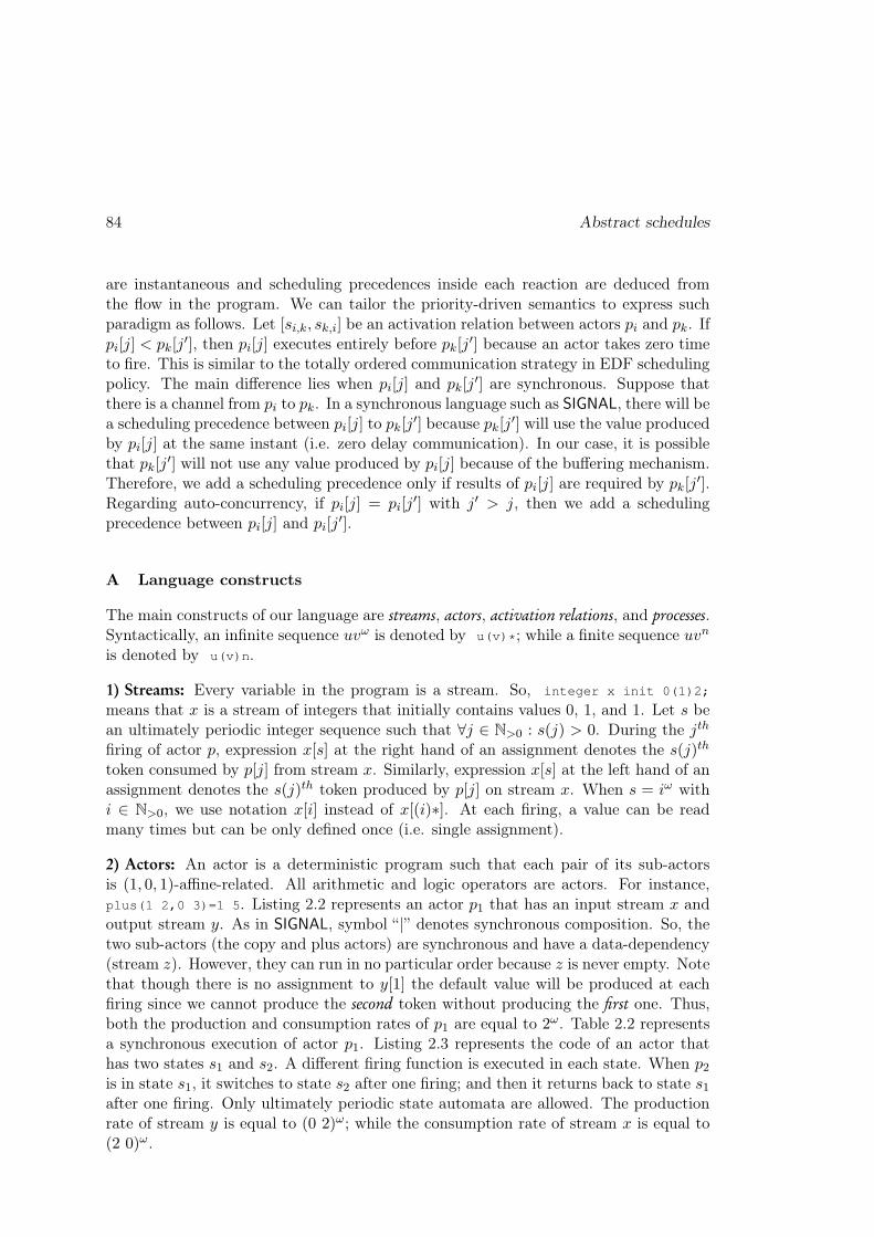
84 Abstract schedules
are instantaneous and scheduling precedences inside each reaction are deduced fromthe flow in the program. We can tailor the priority-driven semantics to express suchparadigm as follows. Let [si,k, sk,i] be an activation relation between actors pi and pk. Ifpi[j] < pk[j
′], then pi[j] executes entirely before pk[j′] because an actor takes zero timeto fire. This is similar to the totally ordered communication strategy in EDF schedulingpolicy. The main difference lies when pi[j] and pk[j
′] are synchronous. Suppose thatthere is a channel from pi to pk. In a synchronous language such as SIGNAL, there will bea scheduling precedence between pi[j] to pk[j′] because pk[j′] will use the value producedby pi[j] at the same instant (i.e. zero delay communication). In our case, it is possiblethat pk[j′] will not use any value produced by pi[j] because of the buffering mechanism.Therefore, we add a scheduling precedence only if results of pi[j] are required by pk[j′].Regarding auto-concurrency, if pi[j] = pi[j
′] with j′ > j, then we add a schedulingprecedence between pi[j] and pi[j′].
A Language constructs
The main constructs of our language are streams, actors, activation relations, and processes.Syntactically, an infinite sequence uvω is denoted by u(v)*; while a finite sequence uvn
is denoted by u(v)n.
1) Streams: Every variable in the program is a stream. So, integer x init 0(1)2;
means that x is a stream of integers that initially contains values 0, 1, and 1. Let s bean ultimately periodic integer sequence such that ∀j ∈ N>0 : s(j) > 0. During the jth
firing of actor p, expression x[s] at the right hand of an assignment denotes the s(j)th
token consumed by p[j] from stream x. Similarly, expression x[s] at the left hand of anassignment denotes the s(j)th token produced by p[j] on stream x. When s = iω withi ∈ N>0, we use notation x[i] instead of x[(i)∗]. At each firing, a value can be readmany times but can be only defined once (i.e. single assignment).
2) Actors: An actor is a deterministic program such that each pair of its sub-actorsis (1, 0, 1)-affine-related. All arithmetic and logic operators are actors. For instance,plus(1 2,0 3)=1 5. Listing 2.2 represents an actor p1 that has an input stream x andoutput stream y. As in SIGNAL, symbol “ |” denotes synchronous composition. So, thetwo sub-actors (the copy and plus actors) are synchronous and have a data-dependency(stream z). However, they can run in no particular order because z is never empty. Notethat though there is no assignment to y[1] the default value will be produced at eachfiring since we cannot produce the second token without producing the first one. Thus,both the production and consumption rates of p1 are equal to 2ω. Table 2.2 representsa synchronous execution of actor p1. Listing 2.3 represents the code of an actor thathas two states s1 and s2. A different firing function is executed in each state. When p2is in state s1, it switches to state s2 after one firing; and then it returns back to state s1after one firing. Only ultimately periodic state automata are allowed. The productionrate of stream y is equal to (0 2)ω; while the consumption rate of stream x is equal to(2 0)ω.

Specific cases 85
Listing 2.2: Actor p1.
actor P1(?real x; ! real y;)
real z init 4.0;
begin
state S1{
y[2]=plus(x[2],z[1]) |
z[1]=x[1]
}
transitions{ }
end
Listing 2.3: Actor p2.
actor P1(?real x; ! real y;)
real z;
begin
state S1{ z[1]=x[1] | z[2]=x[2] }
state S2{ y[2]=z[1] | y[1]=z[2] }
transitions{
S1 -- 1 ->> S2;
S2 -- 1 ->> S1; }
end
Table 2.2: A synchronous execution of actor p1.
firing 1 2 3x = 6 5 4 3 2 1 4 3 2 1 2 1 ǫ
z = 4 6 4 2y = ǫ 0 9 0 9 0 9 0 9 0 9 0 5
3) Activation relations: In a process, every two communicating actors (we assume thatinstances of the same actor have different names) are (1, 0, 1)-affine-related by default.To express a different activation relation between two actors p and q, we use eithernotation p,q=(n,phi,d); to express an affine relation or p,q=[s1,s2]; to express anultimately periodic activation relation.
4) Processes: A process is a multi-clocked composition of actors and processes. Listing2.4 is a process p that consists of the synchronous composition of two [(1 0)ω, (0 2)ω]-activation-related actors p1 and p2. Figure 2.20 represents a synchronous execution ofprocess p.
Listing 2.4: Process p.
process P()
real x init 0.0 1.0; real y;
(|
y=P1(x) | x=P2(y)
|)
where P1,P2=[(1 0)*,(0 2)*];
end
Figure 2.20: A synchronous execution of process p.
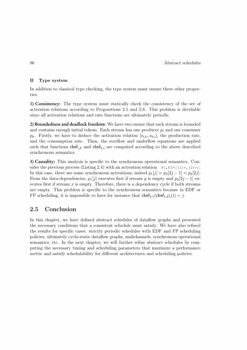
86 Abstract schedules
B Type system
In addition to classical type checking, the type system must ensure three other proper-ties.
1) Consistency: The type system must statically check the consistency of the set ofactivation relations according to Propositions 2.5 and 2.6. This problem is decidablesince all activation relations and rate functions are ultimately periodic.
2) Boundedness and deadlock freedom: We have two ensure that each stream is boundedand contains enough initial tokens. Each stream has one producer pi and one consumerpk. Firstly, we have to deduce the activation relation [si,k, sk,i], the production rate,and the consumption rate. Then, the overflow and underflow equations are appliedsuch that functions cbefi,k and cbefk,i are computed according to the above describedsynchronous semantics.
3) Causality: This analysis is specific to the synchronous operational semantics. Con-sider the previous process (Listing 2.4) with an activation relation P1,P2=[(1)*,(2)*].In this case, there are some synchronous activations; indeed p1[j] = p2[2j − 1] = p2[2j].From the data-dependencies, p1[j] executes first if stream y is empty and p2[2j − 1] ex-ecutes first if stream x is empty. Therefore, there is a dependency cycle if both streamsare empty. This problem is specific to the synchronous semantics because in EDF orFP scheduling, it is impossible to have for instance that cbef2,1(cbef1,2(j)) = j.
2.5 Conclusion
In this chapter, we have defined abstract schedules of dataflow graphs and presentedthe necessary conditions that a consistent schedule must satisfy. We have also refinedthe results for specific cases: strictly periodic schedules with EDF and FP schedulingpolicies, ultimately cyclo-static dataflow graphs, mulichannels, synchronous operationalsemantics, etc. In the next chapter, we will further refine abstract schedules by com-puting the necessary timing and scheduling parameters that maximize a performancemetric and satisfy schedulability for different architectures and scheduling policies.

Chapter 3
Symbolic schedulability analysis
Contents
3.1 General conditions . . . . . . . . . . . . . . . . . . . . . . . . . 87
3.2 Fixed-priority scheduling . . . . . . . . . . . . . . . . . . . . . 90
3.2.1 Priority assignment . . . . . . . . . . . . . . . . . . . . . . . 91
3.2.2 Uniprocessor scheduling . . . . . . . . . . . . . . . . . . . . . 97
3.2.3 Multiprocessor scheduling . . . . . . . . . . . . . . . . . . . . 101
3.3 EDF scheduling . . . . . . . . . . . . . . . . . . . . . . . . . . 102
3.3.1 Deadlines adjustment . . . . . . . . . . . . . . . . . . . . . . 102
3.3.2 Uniprocessor scheduling . . . . . . . . . . . . . . . . . . . . . 106
3.3.3 Multiprocessor scheduling . . . . . . . . . . . . . . . . . . . . 109
3.4 Conclusion . . . . . . . . . . . . . . . . . . . . . . . . . . . . . 112
In real-time scheduling of dataflow graphs, each actor is mapped to a real-time pe-riodic task. The necessary timing parameters that must be computed for each task are:periods, phases, and deadlines. More scheduling parameters could be needed as prior-ities of tasks in FP scheduling and processor allocation in partitioned multiprocessorscheduling. The computed scheduling parameters should respect the abstract schedule,ensure schedulability, and maximize a performance metric.
In the first section, we will present the general conditions that must be satisfiedwhatever the scheduling policy. Then, we present the symbolic schedulability analysisfor two scheduling policies: FP scheduling (Section 3.2) and EDF scheduling (Section3.3).
3.1 General conditions
Let G = (P,E) be a timed static dataflow graph and Gr be the computed affine schedule(or more precisely the graph of affine relations). In a timed dataflow graph, each actorpi is associated with a worst-case execution time sequence ηi ∈ Nω such that ηi[j] is
87

88 Symbolic schedulability analysis
the worst-case execution time of firing pi[j]. To fit the periodic task model, we takethe worst-case execution time of an actor pi as Ci = max
jηi[j]. So, each actor pi is
characterized by (πi, ri, di, Ci) such that πi is the period, ri is the phase, and di is therelative deadline. In FP scheduling, actor pi is permanently assigned the priority wi.The dataflow is to be scheduled on a many-core processor architecture that consists ofM ≥ 1 identical cores. In partitioned scheduling, actor pi is permanently allocated tocore number νi.
An affine relation is an abstract constraint that describes the relative positioningof activations of two actors without considering the physical duration between twoactivations. In the sequel, we will impose that the time interval between successiveactivations of an actor is constant since an actor will be mapped to a periodic task. Letpi and pk be two (n, ϕ, d)-affine-related actors. We have hence that
dπi = nπk (3.1)
rk − ri =ϕ
nπi (3.2)
So, the period and phase of pk can be expressed in terms of the period and phase ofpi; i.e. πk = d
nπi and rk = ri +
ϕnπi. But, timing parameters are non-negative integers.
Thus, πi must be a multiple of lcm{ ngcd{n,d} ,
ngcd{n,ϕ}} and ri must be greater or equal
to −ϕnπi. Similarly, if pi
(n,ϕ,d)−→ pk(n′,ϕ′,d′)−→ pl, then πl = dd′
nn′πi and rl = ri +ϕn′+ϕ′dnn′ πi.
• If the graph of affine relations is connected, then the period of each actor can beexpressed in terms of the period of an arbitrary actor. We can therefore put ∀pi ∈P : πi = αiT where αi ∈ Q>0 and T is a multiple of some integer B. We can also put∀pi ∈ P : ri = f+α′
iT such that f is the phase of the arbitrary actor (f must be greaterthan or equal to max
pi∈P{−α′
iT}). Furthermore, we have that U =∑
pi∈PCiπi
=∑
pi∈PCiαiT
= σT
.
Regardless of the scheduling policy, a necessary condition for schedulability is thatU ≤M . Hence, we have that
T ≥ σ
M(3.3)
For some real-time systems, frequencies of tasks must be higher than some minimalfrequencies under which safety is not ensured or the service quality is poor. The fre-quencies should also be lower than some maximal frequencies over which a device, forexample, may get damage. To better meet these requirements, we allow the designerto specify upper bounds and lower bounds on periods of actors. We will then have thefollowing condition.
T l ≤ T ≤ T u (3.4)
where T l, T u ∈ N>0. The schedulability region concerning the periods and phases isinitially defined by the following constraints: T l ≤ T ≤ T u, T = kB, and T ≥ σ
M. So,
T is the only free variable.
• If the graph of affine relations is disconnected, then we partition Gr to a set of L(maximal) connected graphs Gj = (Pj , Rj). Hence, the period and phase of each actor

General conditions 89
in a partition Pj can be expressed in terms of the period and phase of an arbitraryactor in that partition; i.e. ∀pi ∈ Pj : πi = αiTj and ri = fj + α′
iTj where Tj must bea multiple of Bj , T lj ≤ Tj ≤ T uj , and fj ≥ −α′
iTj . Let U j be the total contribution of
actors in Pj to the processor utilization factor. So, U j =∑
pi∈Pj
Ciπi
=σjTj
. A necessary
schedulability condition is therefore given as
L∑
j=1
σjTj≤M (3.5)
Regarding deadlines, we consider either implicit deadlines or constrained deadlines.The designer may like to impose deadlines. However, since periods are unknown, thedesigner has to specify deadlines in terms of periods; e.g. d1 = π1
2 − 3. Therefore, thedeadline of an actor pi can be expressed in terms of the period of an arbitrary actor inthe connected subgraph that contains pi. So, ∀pi ∈ Pj : di = βiTj − β′i where βi ∈ Q>0
and β′i ∈ N. Since deadlines are integers, βiTj must be an integer. Thus, factor Bj mustbe recomputed. We should also ensure that Ci ≤ di ≤ πi. So,
Ci ≤ βiTj − β′i ≤ αiTj (3.6)
Therefore, the bounds T lj and T uj should also be recomputed.
Regarding priority assignment and processor allocation, these scheduling parametersare required in the affine relation synthesis step and buffer sizes computation. But, inorder to compute them, we need to perform a symbolic schedulability analysis thatrequires performing affine scheduling. We break the cycle in the scheduling approachas follows. Priorities and processor allocation are needed in affine scheduling only tocompute parameters ϕ of affine relations since parameters n and d can be obtainedfrom the boundedness criterion. Parameters ϕ are needed in the symbolic schedulabilityanalysis only to compute phases of actors. But, most schedulability tests consider theworst-case arrival scenario when all actors arrive at the same time. Thus, we do not needparameters ϕ to perform the symbolic schedulability analysis. This slightly influencesthe computation of factors Bj .
Most real-life applications are modeled as connected dataflow graphs. Therefore, wewill focus more on the symbolic schedulability analysis of connected graphs. Obviously,symbolic schedulability analysis of disconnected graphs is more complicated.
Performance metrics
The design process of any embedded real-time system is driven by the objective ofproviding the best possible performance within the timing and resource constraints.Thus, we need to express the performance as a function of the design parameters (freevariables) and then exploring the schedulability region (i.e. the region of the parameterspace that corresponds to feasible designs) to find the best solution. So, if X is thevector of design parameters, S is the schedulability region, and F is the cost (reward or

90 Symbolic schedulability analysis
utility) function, then the symbolic schedulability analysis problem can be formulatedas
maxF (X)
Subject to X ∈ S(3.7)
Many practical cost functions exist such as energy consumption, throughput, la-tency, etc. Some of them could be in conflict with each other as the throughput andbuffering requirements of dataflow graphs. In the rest of this section, we will presentsome cost functions and the controlled parameters for each function. However, we willnot consider metrics that depend on the phases of actors such as the end-to-end latency.
Buffering requirements: As shown in the previous chapter, some scheduling parametersinfluence the buffer sizes computation. In partitioned scheduling, allocating two actorsto the same processor results in a smaller total sum of capacities of the channels be-tween them. In FP scheduling, switching priorities of two actors may improve sizesof buffers between them. In EDF scheduling, adjusting deadlines (to implement thetotally ordered communication strategy) may also reduce the buffering requirements.
Throughput: The throughput of an actor pi is the average number of firings of pi perunit of time and hence equals to its frequency 1
πi. If the graph of affine relations is
connected, then the throughput of the graph is equal to 1πi~r(i)
. The repetition vector ~rcan be easily obtained from parameters n and d of affine relations. Since πi = αiT andU = σ
T, maximizing the throughput is equivalent to maximizing the processor utilization
factor and so to minimizing T .If the graph of affine relations is disconnected (and so the dataflow graph is also
disconnected), the throughput of each connected subgraph Gj can always be expressedin terms of Tj . However, it is not clear how to define the throughput of the whole graph.We hence choose, as in the connected case, to maximize the processor utilization factor.
If T = [T1, . . . , TL] (a lightweight way to denote a vector), then we may considerany cost function F (T ). For most practical metrics, it is expected that the performanceof the system improves when tasks’ rates are increased. Therefore and as in [38], wemy consider cost functions such that ∇F ≤ 0 (i.e. ∀j : ∂F
∂Tj≤ 0). For example,
if F (T ) = U =L∑
j=1
σjTj
, then ∂F∂Tj
=−σjT 2j
≤ 0. Another example is the first order
approximation of the energy spent in a bubble control application which is given as∑
pi∈Paie
− biπi [164].
3.2 Fixed-priority scheduling
In this section, we present the symbolic FP schedulability analysis for uniprocessor andmultiprocessor systems. In each case, we describe the solution with respect to bufferminimization or processor utilization maximization.

Fixed-priority scheduling 91
3.2.1 Priority assignment
We will describe here how to compute the priority of each actor (without computingthe timing parameters) w.r.t. buffer minimization, processor utilization maximization,or a combination of the two metrics. Priorities are used in affine scheduling and theywill be used later to perform a symbolic response time analysis.
A Buffer minimization
Let Ei,k ⊆ E be the set of all channels between pi and pk (in both directions); and letbi,k be the total sum of approximate capacities of channels in Ei,k assuming that pi hasa higher priority than pk (i.e. wi < wk). Table 2.1 (p. 76) shows how to compute theapproximate size of a channel (column νi = νk). So, bi,k =
∑
e∈Ei,k(e)δ(e) such that
wi < wk. For each connected subgraph Gj = (Pj , Ej) in the graph of affine relations,we construct a weighted complete directed graph G′
j = (Pj , E′j) such that the weight of
edge ei,k = (pi, pk) ∈ E′j is equal to bi,k.
Hence, the problem of finding the priority assignment that reduces the bufferingrequirements is equivalent to the linear ordering problem (LOP) [135] which consists infinding an acyclic tournament in the graph G′
j such that the sum of weights of edges inthe tournament is minimal. A tournament is a subset of edges containing for every pairof nodes pi and pk either edge (pi, pk) or (pk, pi) but not both. For N actors, there areN ! different priority assignments (i.e. permutations). The LOP is NP-hard; howevermany exact and heuristic solutions had been proposed in the past decades [135].
The LOP can be formulated as a 0/1 integer linear program. A 0/1 variable xi,kstates whether edge (pi, pk) is present in the tournament or not.
min∑
i,k
bi,k xi,k
∀i < k : xi,k + xk,i = 1
∀i < j, i < k, j 6= k : xi,j + xj,k + xk,i ≤ 2
∀i, k : xi,k ∈ {0, 1}
Once the LOP is solved for every connected subgraph, actors within each subgraphcan be ordered according to the computed priorities. It does not matter how to order twoactors in different subgraphs because this will not influence the buffering requirements.
Example 3.1. Consider the UCSDF example in Figure 2.14 (p. 79) and assume that
all tokens have the same size. The affine relations in the graph are p1(2,ϕ1,4)−→ p2
(6,ϕ2,2)−→p3
(4,ϕ3,6)−→ p1. The graph of affine relations is connected and the constructed weightedgraph for LOP assignment is depicted in Figure 3.1. So, the best priority orderingis p2 p1 p3; while the worst priority ordering is p3 p1 p2 (which is the RM priorityassignment).

92 Symbolic schedulability analysis
Figure 3.1: Priority assignment problem expressed as a LOP.
B Utilization maximization
If deadlines are free parameters, then using implicit deadlines obviously results in thebest utilization. Let us consider the case where deadlines are implicit or user-imposed.In both cases, we have that ∀pi ∈ Pj : di = βiTj − β′i. As mentioned in Chapter 1, theDM priority assignment is optimal (for synchronous task sets). Therefore, it results inthe largest processor utilization. In case of equal deadlines, we break the tie using theactors’ ID. So, the (initial) schedulability region (or the T -space) can be partitionedinto a set of priority regions as illustrated by the following example.
Example 3.2. We add to the UCSDF example (Figure 2.14, p. 79) two actors p4and p5 and a channel e4 = (p4, p5, 4
ω, 1ω). We have hence an additional affine relation
p4(8,ϕ4,2)−→ p5 in graph Gr which is disconnected in this case. So, we have that π =
[T1, 2T1,23T1, T2,
T24 ]. Suppose that C = [65, 70, 95, 60, 55] and d = [π1 − 30, π22 ,
34π3 −
10, π45 , π5 − 60]. We have that U = 242.5T1
+ 280T2
. The initial T -space is hence defined byT1 ≥ 210, T2 ≥ 460, B1 = 6, B2 = 20, and U ≤ 1 (i.e. uniprocessor scheduling). Usinglinear equations di = dk, we can partition the T -space into a set of priority regions asillustrated in Figure 3.2. For instance region S1 corresponds to the DM priority orderingp3 p5 p4 p1 p2.
Definition 3.1 (Monotonicity of schedulability). FP schedulability is monotone overthe T -space if and only if given any two points T1 and T2 in the T -space such thatT1 ≤ T2 and the task set is FP schedulable at T1, then the task set is also FP schedulableat T2.
Property 3.1. Fixed-priority schedulability with predefined priorities is monotoneover the T -space.
Proof: We mean by “predefined” priorities the precomputed priorities that do notdepend on the values of Tj (e.g. the priorities computed for buffer minimization usingLOP assignment). To prove Property 3.1, we use the response time analysis. We have
that Ri = Ci +∑
wi<wk
⌈
Riπk
⌉
Ck. When periods are increased, priorities do not change;
hence, the solution of the recurrence (i.e. the worst-case response time) decreases.Furthermore, the deadline di gets larger since di = βiTj − β′i. So, if Ri was initially lessthan or equal to di, then this remains true when periods are increased.

Fixed-priority scheduling 93
250 300 350 400 450 5500
750
1000
1250
1500
Figure 3.2: Partitioning of the T -space into a set of DM priority regions.
Proposition 3.1. DM schedulability is monotone over the T -space.
Proof: Let T1 and T2 be two points in the T -space such that T1 ≤ T2 and the taskset is DM schedulable at point T1. We denote by πi and di the vectors of periods anddeadlines at point Ti, respectively. We have that π1 ≤ π2 and d1 ≤ d2. There are twocases:1. If T1 and T2 are in the same priority region, then the task set is also DM schedulableat point T2 according to Property 3.1.2. If T1 and T2 are in different priority regions, then we break the transformationfrom the first to the second point into successive swaps as illustrated by the followingexample.
Let π1 = (12, 30, 25, 24), d1 = (5, 20, 21, 24), π2 = (35, 32, 25, 25), and d2 = (27, 26, 21, 25).So, we have that d1 ≤ d2 and π1 ≤ π2. But, T1 and T2 are in different priority regionssince the DM priority ordering at T1 is p1 p2 p3 p4 while the DM priority ordering atpoint T2 is p3 p4 p2 p1. To get from the first permutation (or ordering) to the secondone, we need five swaps (see Figure 3.3).
Since the task set is DM schedulable at the first point, we have only to prove thatit remains DM schedulable after each swap. So, at each step, we switch only prioritiesof pi and pi+1 (assuming that actors are ordered by their priorities). According to theworst-response time computation, we have that
• ∀k > i+1 : Rk remains intact (Actually, Rk decreases if periods πj s.t. j < k areincreased). Hence, ∀k > i+ 1 : pk meets its deadline.
• ∀k < i or k = i+1: Rk decreases or remains intact (note that pi is excluded fromthe sum in the response time formula).

94 Symbolic schedulability analysis
DM
Figure 3.3: Transforming DM priority assignments.
• For pi, we have that Ri = Ci +⌈
Riπi+1
⌉
Ci+1 +∑
k<i
⌈
Riπk
⌉
Ck. Let R′i+1 and d′i+1
be the response time and deadline, respectively, of actor pi+1 before the swap.
So, we have that R′i+1 = Ci+1 +
⌈
R′
i+1
πi
⌉
Ci +∑
k<i
⌈
R′
i+1
πk
⌉
Ck. If we can prove that
Ri ≤ R′i+1, then we will have that Ri ≤ di because di ≥ d′i+1 ≥ R′
i+1.
Since R′i+1 is the fixed point of the response time formula, we have that R′
i+1 =
Ci+1 + aiCi +∑
k<i
akCk such that ∀k ≤ i : ak =⌈
R′
i+1
πk
⌉
∈ N>0. Let us solve the
recurrence for Ri starting from R0i = R′
i+1. So, R1i = Ci +
⌈
R′
i+1
πi+1
⌉
Ci+1 +∑
k<i
akCk.
But, R′i+1 ≤ πi+1 because the system is DM schedulable before the swap. Thus, R1
i =Ci + Ci+1 +
∑
k<i
akCk ≤ R′i+1. We have two cases, either R1
i = R′i+1 (the recurrence
stops) or R1i < R′
i+1. In the second case, we will continue until reaching a fixed pointwhich will be less than R′
i+1.
One direct result of Proposition 3.1 is that if a task is not DM schedulable at pointT2, then it is not DM schedulable at point T1.
C Buffering vs processor utilization
As in static-periodic scheduling of (C)SDF graphs [180], buffer minimization and through-put maximization are in conflict with each other. Indeed, we have shown in Example3.1 that the worst buffering requirements are obtained by the DM priority ordering.This observation can be simply explained as follows. Let pi and pk be two (n, ϕ, d)-affine-related actors with implicit deadlines and all channels between them are directedfrom pi to pk. We have that πk = d
nπi. If d > n, then pi will have a higher DM priority
than pk. But according to Table 2.1 (p. 76), pk must have a higher priority than pi inorder to achieve better buffer sizes.
Let O1 and O2 be two priority orderings (i.e. permutations). The swapping distancebetween O1 and O2 is the minimum number of transpositions of two adjacent elementsnecessary to transform permutation O1 into permutation O2. Each step in the swappingpath positively or negatively affects the buffering requirements and the throughput. Theimpact on buffer sizes can be approximately measured by equations in Table 2.1.

Fixed-priority scheduling 95
Example 3.3. Let us consider the dataflow graph in Figure 2.14 (p. 79). We addtwo actors p4 and p5 and two channels e4 = (p4, p5, 4
ω, 1ω) and e5 = (p5, p3, 1ω, 2ω).
So, π = [T, 2T, 23T,43T,
T3 ], C = [65, 70, 95, 60, 55] and U = 452.5
T. We take deadlines
as d = [π1 − 30, π22 ,34π3 − 10, π42 , π5 − 60]. So, the initial T -space is defined by B = 6
and T ≥ 452.5. Figure 3.4 represents the trade-off between processor utilization andapproximate buffering requirements for all the possible (5!) priority orderings. As onecould notice, many priority orderings can result in the same buffering requirements butin different processor utilizations. If we consider only Pareto points, then the bufferingrequirements and the throughput are proportional to each other.
Figure 3.4: Exploration of the priority orderings space: throughput vs buffering require-ments.
It will be useful if one can compute the (approximate) cost of a swap on the processorutilization without performing a symbolic schedulability analysis. Let O∗, π∗, U∗ bethe DM priority ordering, the period vector, and the processor utilization, respectively,obtained by the symbolic schedulability analysis. Hence, any priority ordering shouldresult in a processor utilization no greater than U∗. Figure 3.5 shows for every priorityordering O the precedence distance between O and O∗ and the corresponding decreasein processor utilization. The precedence distance between two permutations O and O∗
is defined as follows. Let sim(O,O∗) be equal to the number of times an actor pi ispreceded by an actor pk in both O and O∗. The precedence distance is hence equal to
N(N − 1)
2− sim(O,O∗)
If xi,k is the 0/1 variable that states whether actor pi has a higher priority in O∗
than pk or not, then the precedence distance is equal to N(N−1)2 −∑
i,k
xi,k xi,k. In the
ILP formulation, we could add a constraint that states that the precedence distanceis less than some threshold. From Figure 3.5, the decrease in the processor utilizationis roughly proportional to the precedence distance. However, the precedence metric is
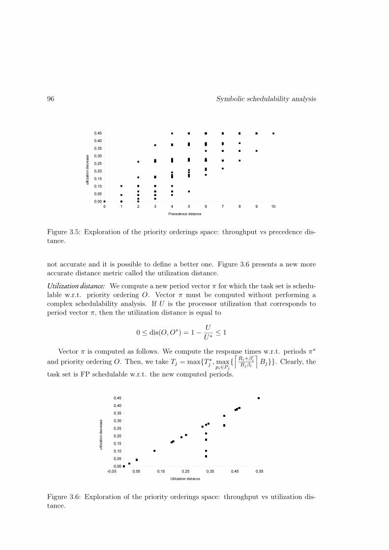
96 Symbolic schedulability analysis
Figure 3.5: Exploration of the priority orderings space: throughput vs precedence dis-tance.
not accurate and it is possible to define a better one. Figure 3.6 presents a new moreaccurate distance metric called the utilization distance.
Utilization distance: We compute a new period vector π for which the task set is schedu-lable w.r.t. priority ordering O. Vector π must be computed without performing acomplex schedulability analysis. If U is the processor utilization that corresponds toperiod vector π, then the utilization distance is equal to
0 ≤ dis(O,O∗) = 1− U
U∗ ≤ 1
Vector π is computed as follows. We compute the response times w.r.t. periods π∗
and priority ordering O. Then, we take Tj = max{T ∗j , max
pi∈Pj{⌈
Ri+β′
i
Bjβi
⌉
Bj}}. Clearly, the
task set is FP schedulable w.r.t. the new computed periods.
Figure 3.6: Exploration of the priority orderings space: throughput vs utilization dis-tance.

Fixed-priority scheduling 97
Heuristic: Many heuristics have beed developed to solve the linear order problem [135].We choose a simple local enumeration method. For a given ordering and a given windowof length W , the heuristic (Algorithm 3) arranges the elements in the window to getthe best buffering requirements and an utilization distance no greater than a thresholdu. We denote by b(O) the sum of approximate buffer sizes w.r.t. priority orderingO. The best ordering among a set of orderings is the one with the smallest bufferingrequirements. In case of tie, we choose the one with the smallest utilization distance.
Algorithm 3: Priority ordering heuristic
O = O∗;repeat
Oprev = O;for i=1, . . ., N-W+1 do
Find the best priority ordering O′ s.t. dis(O′, O∗) ≤ u by arrangingelements at positions i, i+1, . . . , i+W-1 in O;if b(O′) < b(O) or ( b(O′) = b(O) and dis(O′, O∗) < dis(O,O∗) ) then
O = O′;
until Oprev == O;
3.2.2 Uniprocessor scheduling
We firstly consider the simple case where the graph of affine relations is connected andthere is only one priority region (e.g. when deadlines are implicit, the LOP assignment,etc). The maximum throughput corresponds to the minimum value of T . For RMscheduling, we can use the utilization-based tests but they are too pessimistic. There-fore, we will use a symbolic RTA. In the first place, we reduce the space of feasiblevalues of T by using upper and lower bounds on worst-case response times. As shownin Chapter 1,
Rui =
Ci +∑
wk<wi
Ck(1− Uk)
1− ∑
wk<wi
Uk
Following a similar reasoning to that in [40], we can prove that if the system is schedu-lable, then
Rli =
Ci −∑
wk<wi
Ck(1− Uk)
1− ∑
wk<wi
Uk(3.8)
If ∃pi ∈ P : Rli > di, then the task system is unschedulable. We have that
Rli > di ⇔
βiT2 − (Ci + β′i +
∑
wk<wi
Ck(βiαk− 1))T −
∑
wk<wi
Ckαk
(Ck − β′i) < 0
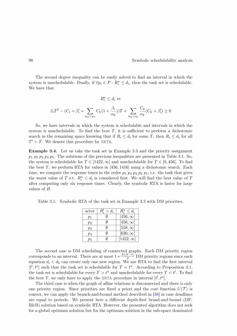
98 Symbolic schedulability analysis
The second degree inequality can be easily solved to find an interval in which thesystem is unschedulable. Dually, if ∀pi ∈ P : Rui ≤ di, then the task set is schedulable.We have that
Rui ≤ di ⇔
βiT2 − (Ci + β′i +
∑
wk<wi
Ck(1 +βiαk
))T +∑
wk<wi
Ckαk
(Ck + β′i) ≥ 0
So, we have intervals in which the system is schedulable and intervals in which thesystem is unschedulable. To find the best T , it is sufficient to perform a dichotomicsearch in the remaining space knowing that if Ri ≤ di for some T , then Ri ≤ di for allT ′ > T . We denote this procedure by SRTA.
Example 3.4. Let us take the task set in Example 3.3 and the priority assignmentp1 p2 p3 p4 p5. The solutions of the previous inequalities are presented in Table 3.1. So,the system is schedulable for T ∈ [1422,∞[ and unschedulable for T ∈ [0, 456[. To findthe best T , we perform RTA for values in [456, 1416] using a dichotomic search. Eachtime, we compute the response times in the order p5 p4 p3 p2 p1; i.e. the task that givesthe worst value of T s.t. Rui ≤ di is considered first. We will find the best value of Tafter computing only six response times. Clearly, the symbolic RTA is faster for largevalues of B.
Table 3.1: Symbolic RTA of the task set in Example 3.3 with DM priorities.
actor Rli > di Rui ≤ dip1 ∅ [456,∞[
p2 ∅ [456,∞[
p3 ∅ [558,∞[
p4 ∅ [630,∞[
p5 ∅ [1422,∞[
The second case is DM scheduling of connected graphs. Each DM priority regioncorresponds to an interval. There are at most 1+ N(N−1)
2 DM priority regions since eachequation di < dk can create only one new region. We use RTA to find the first interval[tl, tu] such that the task set is schedulable for T = tu. According to Proposition 3.1,the task set is schedulable for every T > tu and unschedulable for every T < tl. To findthe best T , we only have to apply the SRTA procedure in interval [tl, tu].
The third case is when the graph of affine relations is disconnected and there is onlyone priority region. Since priorities are fixed a priori and the cost function U(T ) isconvex, we can apply the branch-and-bound method described in [38] in case deadlinesare equal to periods. We present here a different depth-first brand-and-bound (DF-B&B) solution based on symbolic RTA. However, the presented algorithm does not seekfor a global optimum solution but for the optimum solution in the sub-space dominated

Fixed-priority scheduling 99
by a first admissible solution T fst (i.e. for all T in the sub-space, T ≤ T fst). To get theglobal optimum, we have to take T fst = T u. Algorithm 4 represents the pseudo-code ofthe search algorithm.
Algorithm 4: DF-B&B SRTA.
Procedure main() begin
T cur = T fst ;U cur = U(T fst);VisitTree(1);return T cur;
Procedure visitTree(i) begin
ki =PossibleValuesOf(Ti) ;for each t ∈ ki do
if not Feasible(T node) thenprune this node and nodes for remaining values in ki
else
if U(T node) < U cur then
T cur = T node ;U cur = U(T cur);
if i < L then VisitTree(i+1);
In order to explain the algorithm more clearly, we solve the problem in Example3.2 w.r.t. priority ordering p4 p2 p3 p1 p5. Since there are two weakly connectedcomponents, each point in the T -space has two components; i.e. T = [T1, T2]. Thestart point of the algorithm is a first admissible solution T fst (or simply T u, assumingthat the task is schedulable at point T u).
We may compute T fst using a linear relaxation of RTA as follows. Firstly, eachdeadline di = βiTj − β′i is under-approximated as d′i = ρiTj . So, we could simply
take ρi = βi − β′
i
T lj. Clearly, if the system is schedulable with the new deadlines, then
it is schedulable with the original ones. Furthermore, the system is schedulable if
∀pi : Rui =Ci+
∑
wk<wi
Ck
1− ∑
wk<wi
Uk≤ d′i. We solve this problem in R>0 as a linear program by
putting xj = 1Tj
while the objective function is to maximize the processor utilization.
If X = [x1, x2, . . .] is a solution of the linear program, then we take T fstj =
⌈
1xj Bj
⌉
Bj .
Linear programming has a lower time complexity than convex optimization used in[38]. Regarding the previous example, we have that d′ = [67T1, T1,
1942T1,
15T2,
1192T2].
The linear program can hence be written as

100 Symbolic schedulability analysis
max 242.5 x1 + 280 x2
242.5 x1 + 280 x2 ≤ 1 (U ≤ 1)
300 x2 ≤ 1 (Ru4 ≤ d′4)130 x1 + 60 x2 ≤ 1 (Ru2 ≤ d′2)10115 x1 + 1140 x2 ≤ 19 (Ru3 ≤ d′3)3095 x1 + 360 x2 ≤ 6 (Ru1 ≤ d′1)2667.5 x1 + 32400 x2 ≤ 11 (Ru5 ≤ d′5)
0 ≤ x1 ≤1
210; 0 ≤ x2 ≤
1
460
The solution of this program is T fst = [540, 5360] and U fst = 0.501. So, the T -spaceconsists of 13776 points to be checked. From this first admissible solution, the treestructure built by the invocation of visitTree is shown in Figure 3.7. At the first level,procedure PossibleValuesOf(T1) returns all possible values of T1 (denoted by k1) in[T l1, T
fst1 ] such that the system could be schedulable at each point T = [t ∈ k1, T2, . . .]; i.e.
the values of the other components in vector T are constant. Values of ki are obtained
by using test ∀pi : Rli =Ci−
∑
wk<wi
Ck(1−Uk)
1− ∑
wk<wi
Uk≤ di since the system is unschedulable if
∃pi : Rli > di. For the previous example, we have that k1 = [258, 540]. The nodes atthis level are processed in the decreasing order of T1. If the system is unschedulable ata given node, then the subtree whose root is that node will be pruned since, accordingto Property 3.1, reducing values of the other components (i.e. nodes in the subtree) willnot make the system schedulable. For the same raison, we have also to prune all thenodes for the remaining values of T1 in ki. In the example, the system is unschedulablefor T1 = 468 and so for all T1 ∈ [258, 468].
At level L, there is only one free variable, we can hence use SRTA instead of theenumeration to compute the best value of the last component TL.
Figure 3.7: Illustration of DF-B&B symbolic FP schedulability analysis.

Fixed-priority scheduling 101
The fourth and last case is DM scheduling of disconnected graphs. We use the pre-vious branch and bound technique but we have also to consider the DM priority regions.The first admissible solution can be obtained as in the previous case by considering anypriority ordering. Hence, T fst = [474, 2000] (the best solution for priority assignmentp4 p2 p3 p1 p5) is an admissible solution for the DM scheduling. Starting from this point,the space 210 ≤ T1 ≤ 474∧460 ≤ T2 ≤ 2000∧U ≤ 1 contains 9 DM priority regions (seeFigure 3.2). The DF-B&B algorithm can simply be applied on each region. However,this algorithm can be further improved; for instance, by considering Proposition 3.1.For example, Let T be the current node in the current DM priority region, and let T ′
be a node in an already processed region. If T ′ ≥ T and the system is unschedulable inT ′, then the current node can be immediately pruned.
3.2.3 Multiprocessor scheduling
Let us first address the symbolic partitioned scheduling problem. We consider onlyconnected dataflow graphs. Partitioned scheduling is known to be NP-hard; we usetherefore a best fit heuristic that consists in two steps:
1. Order actors by their decreasing priorities. We will consider only systems with aunique priority region (e.g. computed by the LOP priority assignment).
2. Assign each actor (in the previous order) to a processor according to the best fitstrategy.
Let (Vi)i=1,M be the initially empty M partitions (i.e. each partition correspondsto a processor). We allocate task pk, assuming that higher priority tasks are alreadyallocated, as follows. Let Ti be the optimal value (a point in the T -space) returned bythe symbolic response time analysis such that all partitions (Vj)j 6=i and Vi ∪ {pk} areschedulable each one on a single processor. Ti can be found by applying SRTA onlyon partition Vi ∪ {pk} (since partitions (Vj)j 6=i remain schedulable). We assign taskpk to partition Vi that results in the maximum processor utilization U(Ti). In caseof equality, we break the tie by favoring the partition with the minimum utilizationU i =
∑
pj∈Vi∪{pk}
Cjπj
and hence seek for balanced partitions.
ForN periodic tasks, we will apply the symbolic response time analysis N×M times.However, adding task pk to a partition Vi does not change the worst-case response timesof the already allocated tasks on Vi. Hence, if T ′ is the minimum value for which Viis schedulable (which is computed in the previous steps), then T = max{T ′,min{T |Rk ≤ dk}} is the minimum value for which {pk} ∪ Vi is schedulable. If we would like tospeed up more the allocation procedure, we may take T = max{T ′,min{T | Ruk ≤ dk}}as an approximate schedulability test.
Example 3.5. Let us consider the task set in Example 3.3 with priority assignmentp1 p2 p5 p4 p3 and M = 2. Initially, we have that V1 = ∅ and V2 = ∅. Task p1 isassigned directly to partition V1 and task p2 to partition V2; so, V1 = {p1}, V2 = {p2}.At this stage, we have T = 96 and U(T ) = 65
96 + 70192 = 1.041. When allocating task

102 Symbolic schedulability analysis
p5, we have two cases, either to assign the task to partition V1 or to partition V2.In the first case, p1 is already schedulable (for T ≥ 96). We have that T ≥ 96 andR5 = 55+
⌈
R5
T
⌉
65 ≤ d5 implies that T ≥ 540. In the second case, we have that T ≥ 96
and R5 = 55+⌈
R5
2T
⌉
70 ≤ d5 implies that T ≥ 555. So, the best case is to allocate p5 topartition V1 (so, T = 540 and U = 0.78).
This best-fit allocation strategy aims at maximizing the processor utilization. Asshown in the overflow and underflow analyses, the task allocation strategy affects thebuffer sizes computation. Hence, an allocation strategy that reduces the buffering re-quirements can be more suitable for systems with strong memory constraints. Forinstance, a task pk could be assigned to a partition so that the total sum of sizes ofchannels that connect pk to the already assigned tasks is minimized.
For global FP scheduling, we use the schedulability test proposed in [26] (Section1.4.3) assuming that there is a unique priority region. Again, we will consider onlyconnected dataflow graphs. The algorithm consists in arranging tasks by the decreasingorder of priorities. Then, for each task pk and starting from the solution found in theprevious step, we compute the best solution that satisfies Rk ≤ dk. So, we do not haveto check the schedulability of the already processed tasks (thanks to Lemma 3.1).
Lemma 3.1. If T ′ ≥ T , then the value of Rk at T ′ is smaller than its value at T .
Proof: Since Rk = Ck +
⌊
1M
∑
wi<wk
Ii(Rk)
⌋
, it is sufficient to prove that ∀L : Ii(L) is
smaller at T ′ than at T . Recall that Ii(L) is an upper bound on the interference of taskpi on task pk in an interval of length L. This interference is higher for small periodsand deadlines of pi. Hence, Ii(L) at point T ′ is smaller than Ii(L) at point T .
Example 3.6. We again consider the task set in Example 3.3 with priority assignmentp1 p2 p5 p4 p3 and M = 2. For actor p1, we have R1 = 65. Hence, T = 96. Foractor p2, we have that T ≥ 96 and T ≥ R2 = 70 +
⌊
12 min{R2 − 69,W1}
⌋
such thatW1 = N165 + min{65, R2 − T − 95−N1T} and N1 =
⌊
R2+T−95T
⌋
. Hence, T = 96, etc.
3.3 EDF scheduling
In this section, we present the symbolic EDF schedulability analysis of dataflow graphsfor uniprocessor and multiprocessor systems. We also describe the lock-free implemen-tation of the totally ordered communication strategy.
3.3.1 Deadlines adjustment
In FP scheduling, adjusting priorities of actors can be used to reduce the bufferingrequirements. Similarly, adjusting priorities of jobs in EDF scheduling could improve thebuffering requirements, as shown in the previous chapter. Let di[j], Ri[j] = ri+(j−1)πi,and Di[j] = Ri[j] + di[j] be the relative deadline, the release time, and the absolutedeadline of job pi[j], respectively. One way to ensure that job pi[j] has a higher priority
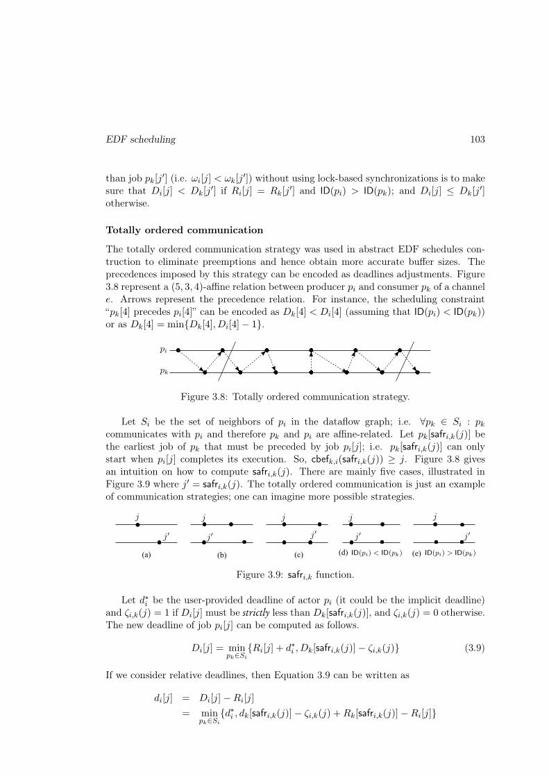
EDF scheduling 103
than job pk[j′] (i.e. ωi[j] < ωk[j′]) without using lock-based synchronizations is to make
sure that Di[j] < Dk[j′] if Ri[j] = Rk[j
′] and ID(pi) > ID(pk); and Di[j] ≤ Dk[j′]
otherwise.
Totally ordered communication
The totally ordered communication strategy was used in abstract EDF schedules con-truction to eliminate preemptions and hence obtain more accurate buffer sizes. Theprecedences imposed by this strategy can be encoded as deadlines adjustments. Figure3.8 represent a (5, 3, 4)-affine relation between producer pi and consumer pk of a channele. Arrows represent the precedence relation. For instance, the scheduling constraint“pk[4] precedes pi[4]” can be encoded as Dk[4] < Di[4] (assuming that ID(pi) < ID(pk))or as Dk[4] = min{Dk[4], Di[4]− 1}.
Figure 3.8: Totally ordered communication strategy.
Let Si be the set of neighbors of pi in the dataflow graph; i.e. ∀pk ∈ Si : pkcommunicates with pi and therefore pk and pi are affine-related. Let pk[safri,k(j)] bethe earliest job of pk that must be preceded by job pi[j]; i.e. pk[safri,k(j)] can onlystart when pi[j] completes its execution. So, cbefk,i(safri,k(j)) ≥ j. Figure 3.8 givesan intuition on how to compute safri,k(j). There are mainly five cases, illustrated inFigure 3.9 where j′ = safri,k(j). The totally ordered communication is just an exampleof communication strategies; one can imagine more possible strategies.
(a) (b) (c) (d) (e)
Figure 3.9: safri,k function.
Let d∗i be the user-provided deadline of actor pi (it could be the implicit deadline)and ζi,k(j) = 1 if Di[j] must be strictly less than Dk[safri,k(j)], and ζi,k(j) = 0 otherwise.The new deadline of job pi[j] can be computed as follows.
Di[j] = minpk∈Si
{Ri[j] + d∗i , Dk[safri,k(j)]− ζi,k(j)} (3.9)
If we consider relative deadlines, then Equation 3.9 can be written as
di[j] = Di[j]−Ri[j]= min
pk∈Si{d∗i , dk[safri,k(j)]− ζi,k(j) +Rk[safri,k(j)]−Ri[j]}

104 Symbolic schedulability analysis
It is worth mentioning that even if pi belongs to a cycle in the dataflow graph,Di[j] does not depend on itself. Therefore, it is possible to compute adjusted deadlinesusing simple propagation of new values. Furthermore, since each affine relation is anultimately periodic activation relation, the deadlines of jobs of each actor are ultimatelyperiodic.
Example 3.7. Consider the UCSDF graph in Figure 2.14 (p. 79) with affine relations
p1(1,1,2)−→ p2
(3,−1,1)−→ p3(2,−1,3)−→ p1. As shown in Figure 3.10, the hyperperiod of this
schedule consists of two activations of p1, one activation of p2, and three activations of p3.Deadlines computation will be limited to one hyperperiod. We have that π = [T, 2T, 23T ]and we suppose that the user-provided deadlines are d∗ = [π1 − 10, π22 , π3] and thatID(p1) < ID(p2) < ID(p3). The new deadlines are computed as follows.
Figure 3.10: Deadlines computation example.
d1[1] = min{d∗1, d3[1] +R3[1]−R1[1]} = T − 10d1[2] = min{d∗1, d2[1], d3[3] +R3[3]−R1[2]} = T − 10d1[3] = min{d∗1, d3[4] +R3[4]−R1[3]} = T − 10d2[1] = min{d∗2, d1[3] +R1[3]−R2[1], d3[3] +R3[3]−R2[1]} = min{T, 2T − 10}d3[1] = d∗3 =
23T
d3[2] = min{d∗3, d1[2]− 1, d2[1]− 1} = min{23T, T − 11}d3[3] = min{d∗3, d1[3] +R1[3]−R3[3]} = min{23T, 43T − 10}d3[4] = d∗3 =
23T
The possible deadline regions are depicted in Table 3.2. So, if C = [65, 70, 95], thenT ≥ 242.5
M. Hence, if M = 1, then ∀pi : di = d∗i .
Table 3.2: Deadline regions of Example 3.7.
T ∈ ]10, 15] ]15, 33] ]33,∞[
d1 (T − 10)ω (T − 10)ω (T − 10)ω
d2 (T )ω (T )ω (T )ω
d3 2
3T (T − 11 4
3T − 10 2
3T )ω 2
3T (T − 11 2
3T 2
3T )ω (23T )
ω
Approximate deadlines
Most of EDF schedulability tests assume that a task has a unique deadline. To fit inthis model, we may consider the following two simple solutions.
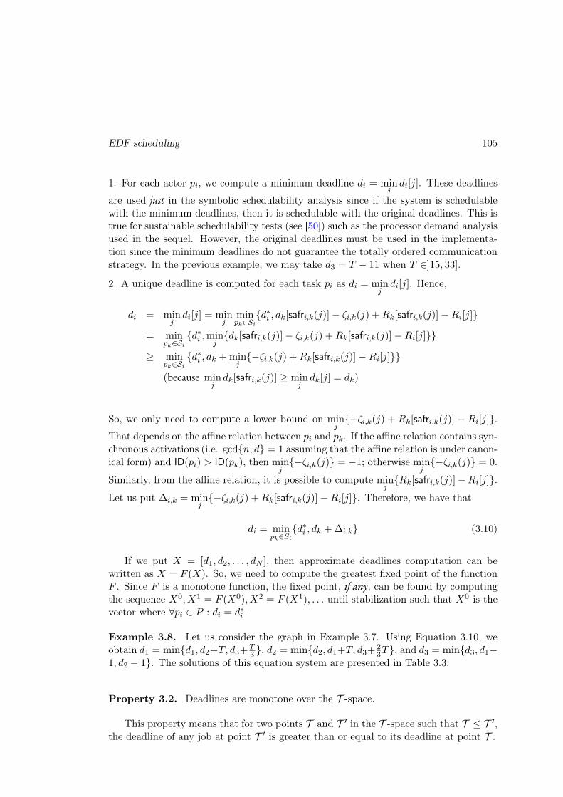
EDF scheduling 105
1. For each actor pi, we compute a minimum deadline di = minjdi[j]. These deadlines
are used just in the symbolic schedulability analysis since if the system is schedulablewith the minimum deadlines, then it is schedulable with the original deadlines. This istrue for sustainable schedulability tests (see [50]) such as the processor demand analysisused in the sequel. However, the original deadlines must be used in the implementa-tion since the minimum deadlines do not guarantee the totally ordered communicationstrategy. In the previous example, we may take d3 = T − 11 when T ∈]15, 33].2. A unique deadline is computed for each task pi as di = min
jdi[j]. Hence,
di = minjdi[j] = min
jminpk∈Si
{d∗i , dk[safri,k(j)]− ζi,k(j) +Rk[safri,k(j)]−Ri[j]}
= minpk∈Si
{d∗i ,minj{dk[safri,k(j)]− ζi,k(j) +Rk[safri,k(j)]−Ri[j]}}
≥ minpk∈Si
{d∗i , dk +minj{−ζi,k(j) +Rk[safri,k(j)]−Ri[j]}}
(because minjdk[safri,k(j)] ≥ min
jdk[j] = dk)
So, we only need to compute a lower bound on minj{−ζi,k(j) + Rk[safri,k(j)] − Ri[j]}.
That depends on the affine relation between pi and pk. If the affine relation contains syn-chronous activations (i.e. gcd{n, d} = 1 assuming that the affine relation is under canon-ical form) and ID(pi) > ID(pk), then min
j{−ζi,k(j)} = −1; otherwise min
j{−ζi,k(j)} = 0.
Similarly, from the affine relation, it is possible to compute minj{Rk[safri,k(j)]−Ri[j]}.
Let us put ∆i,k = minj{−ζi,k(j) +Rk[safri,k(j)]−Ri[j]}. Therefore, we have that
di = minpk∈Si
{d∗i , dk +∆i,k} (3.10)
If we put X = [d1, d2, . . . , dN ], then approximate deadlines computation can bewritten as X = F (X). So, we need to compute the greatest fixed point of the functionF . Since F is a monotone function, the fixed point, if any, can be found by computingthe sequence X0, X1 = F (X0), X2 = F (X1), . . . until stabilization such that X0 is thevector where ∀pi ∈ P : di = d∗i .
Example 3.8. Let us consider the graph in Example 3.7. Using Equation 3.10, weobtain d1 = min{d1, d2+T, d3+ T
3 }, d2 = min{d2, d1+T, d3+ 23T}, and d3 = min{d3, d1−
1, d2 − 1}. The solutions of this equation system are presented in Table 3.3.
Property 3.2. Deadlines are monotone over the T -space.
This property means that for two points T and T ′ in the T -space such that T ≤ T ′,the deadline of any job at point T ′ is greater than or equal to its deadline at point T .
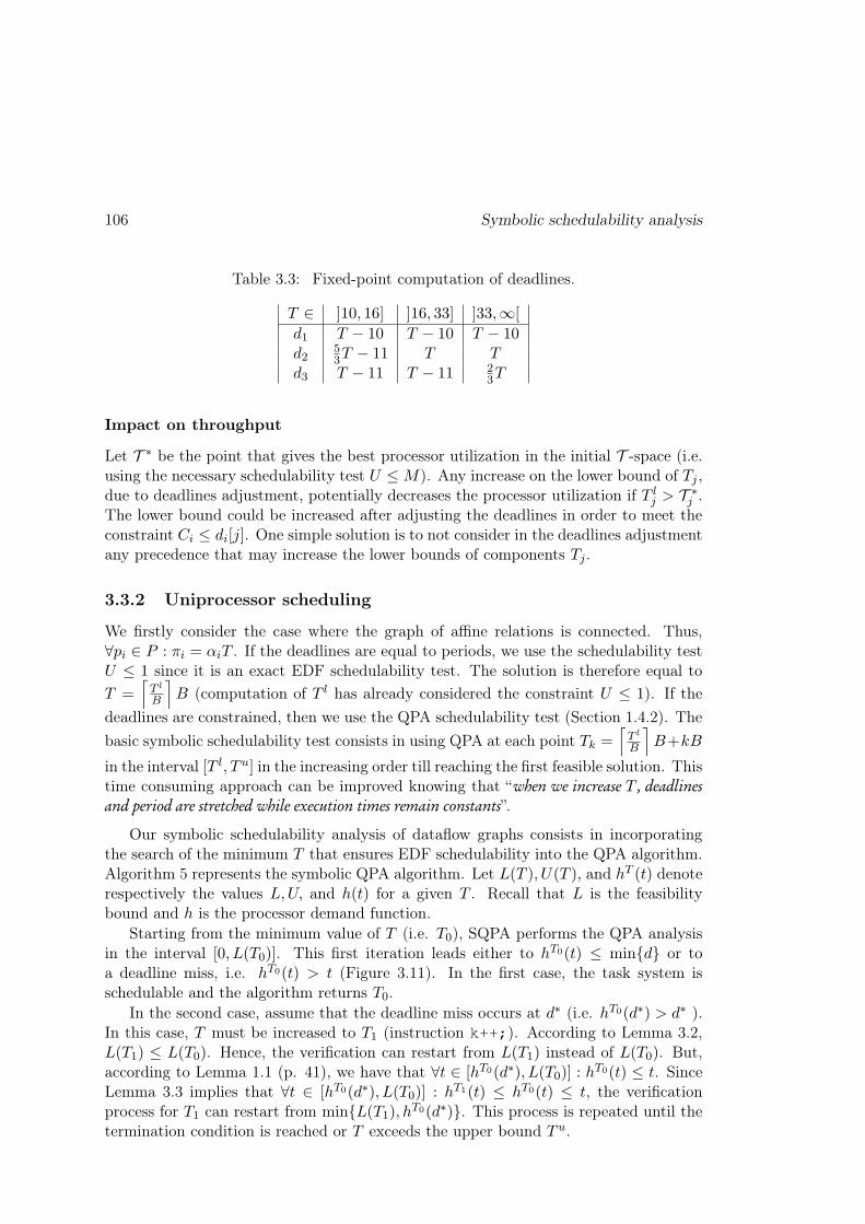
106 Symbolic schedulability analysis
Table 3.3: Fixed-point computation of deadlines.
T ∈ ]10, 16] ]16, 33] ]33,∞[
d1 T − 10 T − 10 T − 10d2
53T − 11 T T
d3 T − 11 T − 11 23T
Impact on throughput
Let T ∗ be the point that gives the best processor utilization in the initial T -space (i.e.using the necessary schedulability test U ≤M). Any increase on the lower bound of Tj ,due to deadlines adjustment, potentially decreases the processor utilization if T lj > T ∗
j .The lower bound could be increased after adjusting the deadlines in order to meet theconstraint Ci ≤ di[j]. One simple solution is to not consider in the deadlines adjustmentany precedence that may increase the lower bounds of components Tj .
3.3.2 Uniprocessor scheduling
We firstly consider the case where the graph of affine relations is connected. Thus,∀pi ∈ P : πi = αiT . If the deadlines are equal to periods, we use the schedulability testU ≤ 1 since it is an exact EDF schedulability test. The solution is therefore equal to
T =⌈
T l
B
⌉
B (computation of T l has already considered the constraint U ≤ 1). If the
deadlines are constrained, then we use the QPA schedulability test (Section 1.4.2). The
basic symbolic schedulability test consists in using QPA at each point Tk =⌈
T l
B
⌉
B+kB
in the interval [T l, T u] in the increasing order till reaching the first feasible solution. Thistime consuming approach can be improved knowing that “when we increase T , deadlinesand period are stretched while execution times remain constants”.
Our symbolic schedulability analysis of dataflow graphs consists in incorporatingthe search of the minimum T that ensures EDF schedulability into the QPA algorithm.Algorithm 5 represents the symbolic QPA algorithm. Let L(T ), U(T ), and hT (t) denoterespectively the values L,U, and h(t) for a given T . Recall that L is the feasibilitybound and h is the processor demand function.
Starting from the minimum value of T (i.e. T0), SQPA performs the QPA analysisin the interval [0, L(T0)]. This first iteration leads either to hT0(t) ≤ min{d} or toa deadline miss, i.e. hT0(t) > t (Figure 3.11). In the first case, the task system isschedulable and the algorithm returns T0.
In the second case, assume that the deadline miss occurs at d∗ (i.e. hT0(d∗) > d∗ ).In this case, T must be increased to T1 (instruction k++;). According to Lemma 3.2,L(T1) ≤ L(T0). Hence, the verification can restart from L(T1) instead of L(T0). But,according to Lemma 1.1 (p. 41), we have that ∀t ∈ [hT0(d∗), L(T0)] : hT0(t) ≤ t. SinceLemma 3.3 implies that ∀t ∈ [hT0(d∗), L(T0)] : hT1(t) ≤ hT0(t) ≤ t, the verificationprocess for T1 can restart from min{L(T1), hT0(d∗)}. This process is repeated until thetermination condition is reached or T exceeds the upper bound T u.

EDF scheduling 107
increase Tupdate
schedulable
Figure 3.11: Illustration of SQPA.
Algorithm 5: SQPA algorithm
k = 0; t = max{d|d ≤ L(Tk)};while h(t) > min{d} do
if h(t) < t then t = h(t);else if t == h(t) then t = max{d|d < t};else
k++;if Tk > T u then return task set not schedulable;t = min{hTk−1(t),max{d|d ≤ L(Tk)}};
return Tk;
Lemma 3.2. If T ≤ T ′, then L(T ) ≥ L(T ′).
Proof: We have that L is equal to synchronous busy period which can computed with
Lm+1 =∑
pi∈P
⌈
Lm
πi
⌉
Ci where L0 =∑
pi∈PCi. Clearly, ∀m : Lm(T ′) ≤ Lm(T ). Hence,
L(T ′) ≤ L(T ).
Lemma 3.3. If T ≤ T ′, then ∀t : hT (t) ≥ hT ′
(t).
Proof: We have that hT (t) =∑
pi∈PhTi (t) such that hTi (t) =
∑
Di[j]≤tCi. According to
Property 3.2, a given absolute deadline occurs earlier for T than for T ′. Therefore,∀l, hTi (t) ≥ hT
′
i (t).SQPA algorithm has a pseudo-polynomial complexity since it checks in the worst-
case scenario all the deadlines in interval [0, L(T0)] as a standard processor-demandanalysis may do.
Example 3.9. We take the same example as in Example 3.7 with C = [65, 70, 95]. Wehave that U = 242.5
T, T ≥ 243, and B = 3.
• T = 243, L = 485t = 476, h(t) = 390 t = 390, h(t) = 325t = 325, h(t) = 325 t = 324, h(t) = 325 (deadline miss; increase T )• T = 246, L = 485t = 325, h(t) = 230 t = 230, h(t) = 95 (return T = 246)

108 Symbolic schedulability analysis
So, the maximum processor utilization that can be achieved with the user-provideddeadlines is equal to U = 0.985.
The second case is when the graph of affine relations is disconnected. We proposea DF-B&B SQPA search algorithm (Algorithm 6). Procedure SQPA∗(T , t) performsQPA (i.e. testing h(t) ≤ t in backward manner) for a given value T starting frompoint min{t, L(T )}. It ends when there is a miss (i.e. this procedure does not increaseperiods) or if the system is schedulable at point T . When U(T ) > 1, the procedureindicates the miss immediately. To better explain the search algorithm, we consider thefollowing example.
Algorithm 6: DF-B&B SQPA.
Procedure main() begin
T cur = [T l1, . . . , TlL]; U
cur = 0;t = SQPA∗(T cur, L(T cur));if t > min{d} then VisitTree(T cur, t, 1);return T cur;
Procedure visitTree(T , t, j) begin
for i = j, j + 1, . . . ,L, . . . , j − 1 do
T node ← increase Ti in T ;if Ti > T ui or U(T node) ≤ U cur then prune this node;else
t = SQPA∗(T node, t) ;if t ≤ min{d} then T cur = T node; U cur = U(T node);
else VisitTree(T node, hTnode
(t), j mod L+ 1);
Example 3.10. Let us take the dataflow graph in Example 3.2 with C = [20, 30, 10, 15, 10]and d = [π1 − 30, π22 − 5, π3, π4 − 5, 45π5 − 10]. We have that π = [T1, 2T1,
23T1, T2,
T24 ].
We suppose that the initial T -space is defined by T1 ≥ 84, T2 ≥ 100, B1 = 12, B2 = 20,and U = 50
T1+ 55
T2≤ 1.
Figure 6 represents the results of the search algorithm where nodes are numberedin the order of appearance. Initially, we have that T cur = [102, 96] and U = 0. SinceU(T cur) > 1, procedure SQPA∗ indicates a miss immediately. From each node, weincrease either T1 or T2. The first node with U(T node) ≤ 1 is T node = [96, 120]. At thisnode, Procedure SQPA∗ returns a miss. As in SQPA, If d∗ is the missed deadline, thenthe verification will continue from min{L, h(d∗)} when periods are increased (h(d∗) isdenoted by t in Figure 3.12). The first encountered leaf is T = [120, 160] (i.e. thetask set is EDF-schedulable at this point), and U cur and T cur must be updated. Nodenumbered 12 is pruned because U([144, 120]) < U cur = 0.806.
However, this algorithm requires upper bounds T uj in order to have a finite searchspace. This is mainly to ensure that a point such T = [∞, T l2] or T = [T l1,∞] cannot
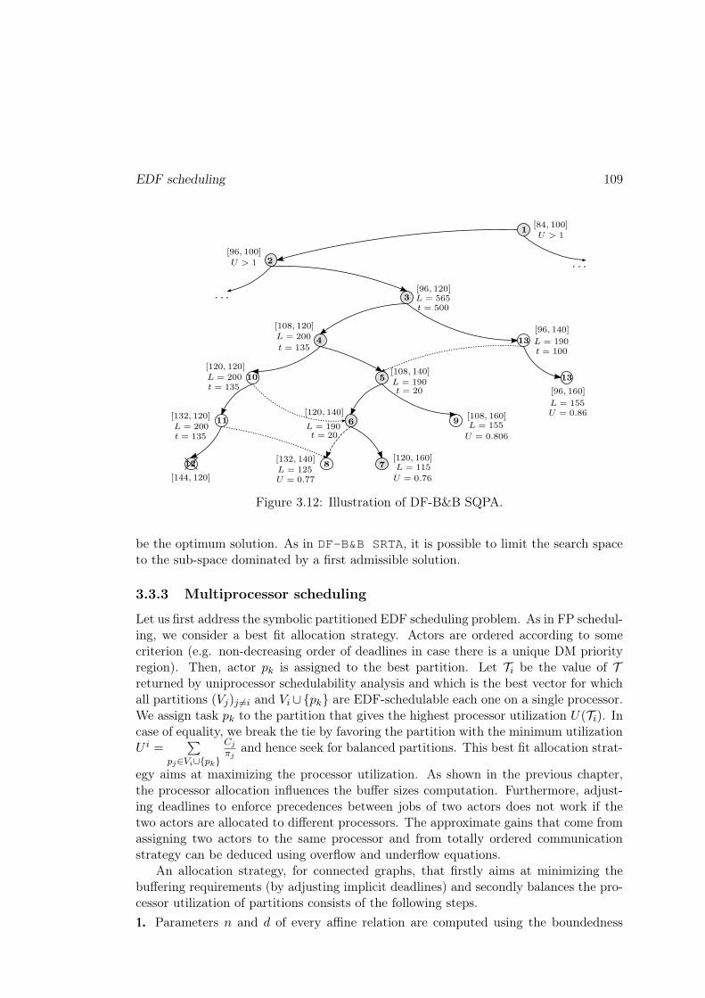
EDF scheduling 109
Figure 3.12: Illustration of DF-B&B SQPA.
be the optimum solution. As in DF-B&B SRTA, it is possible to limit the search spaceto the sub-space dominated by a first admissible solution.
3.3.3 Multiprocessor scheduling
Let us first address the symbolic partitioned EDF scheduling problem. As in FP schedul-ing, we consider a best fit allocation strategy. Actors are ordered according to somecriterion (e.g. non-decreasing order of deadlines in case there is a unique DM priorityregion). Then, actor pk is assigned to the best partition. Let Ti be the value of Treturned by uniprocessor schedulability analysis and which is the best vector for whichall partitions (Vj)j 6=i and Vi ∪{pk} are EDF-schedulable each one on a single processor.We assign task pk to the partition that gives the highest processor utilization U(Ti). Incase of equality, we break the tie by favoring the partition with the minimum utilizationU i =
∑
pj∈Vi∪{pk}
Cjπj
and hence seek for balanced partitions. This best fit allocation strat-
egy aims at maximizing the processor utilization. As shown in the previous chapter,the processor allocation influences the buffer sizes computation. Furthermore, adjust-ing deadlines to enforce precedences between jobs of two actors does not work if thetwo actors are allocated to different processors. The approximate gains that come fromassigning two actors to the same processor and from totally ordered communicationstrategy can be deduced using overflow and underflow equations.
An allocation strategy, for connected graphs, that firstly aims at minimizing thebuffering requirements (by adjusting implicit deadlines) and secondly balances the pro-cessor utilization of partitions consists of the following steps.
1. Parameters n and d of every affine relation are computed using the boundedness

110 Symbolic schedulability analysis
criterion. So, we have that ∀pi ∈ P : πi = αiT .
2. Let G = (V,E) be an undirected graph where nodes represent actors and edgesrepresent affine relations. Each node vi is associated with a weight that represents theutilization of actor pi; i.e. w(vi) = Ci
αi. The weight of edge ei,k = (vi, vk), denoted
by w(ei,k), is equal to zero if enforcing precedences between pi and pk may jeopardizethe processor utilization factor, and equal to the approximate gain that comes fromadjusting the deadlines otherwise.
3. The graph G should be partitioned into M balanced partitions (Vi)i=1,M ; thatis, ∀i, j : |w(Vi) − w(Vj)| is minimal such that w(Vi) =
∑
v∈Viw(v). Furthermore, the
partitioning must minimize the total weight of edges connecting different partitions. Thereason behind this requirement is that adjusting deadlines will not ensure precedencesbetween actors allocated to different processors. This M -partitioning problem is wellknown in graph theory; for instance, we use the SCOTCH tool [59] to solve the problem.
4. Once each actor is assigned to a processor, overflow and underflow analyses can beperformed to compute parameter ϕ of each affine relation.
5. Computation of symbolic deadlines of tasks in each partition.
6. The SQPA algorithm is then applied on each partition Vi. The algorithm will returnthe minimum value Ti that ensures EDF schedulability of the set Vi on a single processor.We need just to take T = max
i=1,MTi.
For global EDF scheduling of connected graphs, we will use the QPA-FFDBF schedu-lability test. But first, we propose an improvement of the schedulability test using thefollowing lemma.
Lemma 3.4. If γ1 < γ2 and ffdbf(t, γ1) ≥ (M−(M−1)γ1(M−1)γ2
)∑
pi∈PCi, then h(t, γ1) ≤ h(t, γ2).
Proof: Figure 3.13 depicts the forced-forward demand bound function for two values γ1and γ2 such that γ1 < γ2. As shown in that figure, we have clearly that ∀t : 0 ≤ ∆i(t) =ffdbfi(t, γ1) − ffdbfi(t, γ2) ≤ ∆i. Using basic geometry, we have that ∆i = Ci(1 − γ1
γ2).
So,
hi(t, γ2)− hi(t, γ1) =ffdbf
i(t, γ1)−∆i(t)
M − (M − 1)γ2− ffdbf
i(t, γ1)
M − (M − 1)γ1
Hence,
h(t, γ2)− h(t, γ1) =x
(M − (M − 1)γ2)(M − (M − 1)γ1)
s.t. x = (M − 1)(γ2− γ1) ffdbf(t, γ1)− (M − (M − 1)γ1)∑
pi∈P∆i(t). Therefore, if x ≥ 0;
i.e.
ffdbf(t, γ1) ≥M − (M − 1)γ1(M − 1)(γ2 − γ1)
∑
pi∈P∆i(t)
then h(t, γ1) ≤ h(t, γ2). But, ∀t : ∑
pi∈P∆i(t) ≤
∑
pi∈P∆i.

EDF scheduling 111
Figure 3.13: Illustration of ffdbf
Lemma 3.4 is used as follows. For a given γ1, if h(t, γ1) > t and ffdbf(t, γ1) ≥ F ∗ =
(M−(M−1)γ1(M−1)γ1
)∑
pi∈PCi, then it does not matter if we increase γ1 to γ2 since h(t, γ2) will
be also greater than t. Note that we used γ1 in the dominator of F ∗ instead of γ2.
Algorithm 7 represents the symbolic QPA-FFDBF algorithm for global EDF schedul-ing of connected graphs. Let γmin(T ), and γmax(T ) denote respectively γmin = µ∗, andγmax = M−U
M−1 for a given T . Let F ∗(γ) denote the value of F ∗ for a given value of γ. Ifh(t, γ) > t, then we have to increase either γ or T according to Lemma 3.4 and Theorem1.2 (p. 42). As for SQPA, we note the following results.
Lemma 3.5. If T ≤ T ′, then ∀t : hT (t, γ) ≥ hT ′
(t, γ).
Proof: We have that hT (t, γ) =
∑
pi∈P
ffdbf Ti (t,γ)
M−(M−1)γ . It is quite easy to prove that ffdbf T′
i (t, γ) ≤ffdbf Ti (t, γ). Indeed, periods and deadlines are larger at point T ′ than at point T . Youcan easily notice in Figure 3.13 that the value of the forced-forward demand boundfunction decreases when periods and deadlines are increased.
If d∗ is the first deadline for which hT (d∗, γ) > d∗, then we have that ∀t ∈ [hT (d∗, γ), L(T )] :hT
′
(t, γ) ≤ hT (l, γ) ≤ t. For given values Tk+1 and γ, we take Prev(γ) = hTk(d∗, γ).
Lemma 3.6. If T ≤ T ′, then L(T ) ≥ L(T ′).
Proof: If there is a unique deadline region and ∀pi : diπi is monotone over the T -space,
then L =
∑
pi∈P
(πi−di)Ui
M−(M−1)γ−U satisfies the property; otherwise L =
∑
pi∈P
Ci
M−(M−1)γ−U (from [11])satisfies the property.
Thanks to these observations, for a given value γ, it is not necessary to recheckdeadlines in the interval [L(T ′),Prev(γ)] when T is increased to T ′.
It is worth mentioning that computation of T l must consider the constraint µ∗ <M−UM−1 . If the graph of affine relation is disconnected, then a branch and bound techniquelike the one proposed for SQPA can be used with SQPA-FFDBF.

112 Symbolic schedulability analysis
Algorithm 7: SQPA-FFDBF algorithm
k = 0; γ = γmin(Tk); t = L(Tk);while h(t, γ) > min{d} do
if h(t, γ) ≤ t then t = min{h(t, γ),max{d|d < t}};else
if ffdbf(t, γ) ≥ F ∗(γ) ∨ γ + ǫ ≥ γmax(Tk) then
k++;if Tk > T u then return task set unschedulable;γ = γmin(Tk);
else γ = γ + ǫ;t = min{L(Tk),Prev(γ)};
return Tk;
Example 3.11. Let us consider the task set in Example 3.3: π = [T, 2T, 23T,43T,
T3 ],
C = [65, 70, 95, 60, 55], d = [π1 − 30, π22 ,34π3 − 10, π42 , π5 − 60], and U = 452.5
T. If
M = 2, then the initial T -space is defined by T ≥ 348 and B = 6. We have thatγmin(T ) = max{ 190
T−20 ,165
T−180} and γmax(T ) = 2 − 452.5T
. Constraint µ∗ < M−UM−1 implies
that T ≥ 384. We take ǫ = 0.002 and the initial value of γ is rounded up (e.g.0.6893→ 0.690) in order to pass by the same values of γ in the iterations.
✷ T = 384, γmin = 0.8088, γmax = 0.8216• γ = 0.810, L = 10504t = 10504, h(t, γ) = 10425.21 t = 10425, h(t, γ) = 10363.86 . . .t = 6584, h(t, γ) = 6584.03: miss.Increasing γ will not solve the problem since ffdbf (t, γ) = 7835.0 > F ∗ = 506.85. Hence,T must be increased.✷ T = 390, γmin = 0.7857, γmax = 0.8397• γ = 0.786, L = 2270t = 2265, h(t, γ) = 2173.49 . . . t = 751, h(t, γ) = 751.23: miss and ffdbf (t, γ) > F ∗....✷ T = 408, γmin = 0.7236, γmax = 0.8909
• γ = 0.724, L = 718: schedulable and UM
= 0.554
3.4 Conclusion
In this chapter, we have presented the necessary symbolic schedulability analyses ofabstract schedules that aim at either minimizing the buffering requirements or maxi-mizing the processor utilization. We have presented the symbolic schedulability analysisfor uniprocessor and multiprocessor systems with respect to two real-time schedulingpolicies: fixed-priority scheduling and earliest-deadline first scheduling.

Chapter 4
Experimental validation
Contents
4.1 Performance comparison: ADFG vs DARTS . . . . . . . . . . 113
4.1.1 Throughput . . . . . . . . . . . . . . . . . . . . . . . . . . . . 115
4.1.2 Buffering requirements . . . . . . . . . . . . . . . . . . . . . . 118
4.2 Symbolic schedulability analysis . . . . . . . . . . . . . . . . 121
4.2.1 EDF scheduling . . . . . . . . . . . . . . . . . . . . . . . . . . 122
4.2.2 Fixed-priority scheduling . . . . . . . . . . . . . . . . . . . . 125
4.3 Application: Design of SCJ/L1 systems . . . . . . . . . . . . 127
4.3.1 Concurrency model of SCJ/L1 . . . . . . . . . . . . . . . . . 128
4.3.2 Dataflow design model . . . . . . . . . . . . . . . . . . . . . . 129
4.4 Conclusion . . . . . . . . . . . . . . . . . . . . . . . . . . . . . 131
In this chapter, we present the results obtained by the scheduling algorithms on aset of real-life stream processing applications and randomly generated dataflow graphsw.r.t. buffer minimization and throughput maximization. Furthermore, we comparethe complexity of our symbolic schedulability analyses with that of basic enumerativesolutions. We refer to the implementation of our scheduling algorithms as the ADFG
tool. We will also briefly present a graphical editor for automatic synthesis of SCJ Level1 applications from UCDF graph specifications.
4.1 Performance comparison: ADFG vs DARTS
In a first place, we compare our scheduling tool (the ADFG tool) with the DARTS tool(an implementation of the scheduling approach presented in [9]). In the best of ourknowledge, DARTS is the only existing tool for real-time scheduling of (C)SDF graphs.However, it can handle only acyclic connected graphs. Therefore, we use the same acyclicbenchmarks (see Table 4.1) presented in more details in [9]. They are SDF and CSDFgraphs collected from many sources (the StreamIt benchmark [190], the SDF3 tool [182],
113

114 Experimental validation
Application #nodes #edges B σ Θ(G) Umax minBS
Serpent 120 128 1 129020 2.99× 10⁻⁴ 38.675 14249Fast Fourier transform (FFT) 17 16 1 141058 8.31× 10⁻⁵ 11.723 8192MPEG2 video 23 26 1 56737 1.30× 10⁻⁴ 7.387 6274Digital Radio Mondiale receiver 4 3 768 47207.8 1.24× 10⁻⁵ 2.927 2698Channel vocoder 55 70 1 1186025 2.81× 10⁻⁵ 33.409 2618Data Encryption Standard (DES) 53 60 1 18034 9.76× 10⁻⁴ 17.611 2564Discrete cosine transform (DCT) 8 7 1 121672 2.10× 10⁻⁵ 2.555 1792Satellite receiver 22 26 220 188.12 9.45× 10⁻⁴ 4.275 1542H.263 video decoder 4 3 1 1107.24 3.01× 10⁻⁶ 1.98 1189Filterbank for signal processing 85 99 1 364268 8.84× 10⁻⁵ 32.201 680Vocoder 114 146 1 25417 1.10× 10⁻⁴ 2.791 668Multi-channel beamformer 57 70 1 130033 1.97× 10⁻⁴ 25.617 254Bitonic Parallel Sorting 40 46 1 930 1.05× 10⁻² 9.789 151Software FM radio with equalizer 43 53 1 18828 6.97× 10⁻⁴ 13.129 57Heart pacemaker 4 3 320 611 3.12× 10⁻³ 1.909 42MP3 audio decoder 14 18 1 6105381 2.68× 10⁻⁷ 3.271 20Data modem 6 5 1 2.93 6.25× 10⁻² 2.937 16CD-to-DAT rate converter 6 5 80 16.36 8.50× 10⁻⁴ 4.227 5
Table 4.1: Real-life stream processing benchmarks.
and some research papers). The number of nodes in a graph is denoted by #nodes,the number of channels is denoted by #edges, the maximum throughput (i.e. theself-timed throughput) is denoted by Θ(G), while the minimum buffering requirementsthat can be obtained by a static-periodic schedule is denoted by minBS. The maximumthroughput and the minimum buffering requirements are computed after disabling auto-concurrency. Minimum buffering requirements are computed using the SDF3 tool. Thethroughput of an actor pi is taken as Θ(pi) = Θ(G)~r(i). Then, the maximum processorutilization is taken as Umax =
∑
pi∈PΘ(pi)Ci.
Definition 4.1. Let e = (pi, pk, u1vω1 , u2v
ω2 ) be a channel. Channel e is said to be a
matched I/O rates channel if ‖v1‖|v1| ≈
‖v2‖|v2| . It is said to be a perfectly matched I/O rates
channel if ‖v1‖|v1| = ‖v2‖
|v2| .
If all the channels in a graph are perfectly matched I/O rates channels, then fac-tor B (computed in the symbolic schedulability analysis) will be equal to 1. Most ofthe applications in Table 4.1 (except for MP3 decoder, cd2dat-csdf, Satellite,Receiver, and Pacemaker) consist of perfectly matched I/O rates channels. Thiskind of graphs does not allow us to demonstrate the reduction of buffering requirementsthat results from priority assignment or deadlines adjustment because of the followingobservation. According to Table 2.1, the approximate gain that comes from switchingthe priorities of the producer and the consumer is given as ‖v2‖
|v2|∣
∣
d−nn
∣
∣. But, this quantity

Performance comparison: ADFG vs DARTS 115
is very small in case of matched I/O rates channels (and null in case of perfectly matchedI/O channels) since d
n= ‖v1‖
|v1||v2|‖v2‖
. Similar observation holds for deadlines adjustment.To better measure the impact of our techniques, we will use a set of randomly generated(cyclic) connected SDF graphs. The graphs are generated by the SDF3 tool with thefollowing setting. Production and consumption rates follow a normal distribution witha mean equal to 5 and a variance equal to 4. Worst-case execution times follow a normaldistribution with a mean equal to 1000 and a variance equal to 300. The graphs aregenerated with different numbers of nodes (from 6 to 80) such that the average degreeof each node is 2.
In most of the experiments, we will assume implicit deadlines unless it is stated oth-erwise or the deadlines adjustment technique is used. We will show the results obtainedby some of the scheduling algorithms presented in the previous chapter. However, wewill focus more on uniprocessor scheduling algorithms.
4.1.1 Throughput
We consider here some of the scheduling algorithms that aim at maximizing the pro-cessor utilization regardless of the achieved buffering requirements. Let us first addressthe uniprocessor scheduling case.
Figure 4.1 shows the obtained results by the ADFG and DARTS tools in case of EDFand FP priority scheduling of the real-life benchmarks. Implicit deadlines are used inorder to achieve the highest throughput. Furthermore, the priority assignment policyfor FP scheduling is taken as the RM priority assignment. Clearly, our scheduling toolgives (by far) the best processor utilization in case of RM scheduling. This is because ourRM schedulability analysis is based on the accurate RTA; while the RM schedulabilityanalysis in the DARTS tool is based on the pessimistic utilization-based test.
!"!#$"!#%"!#&"!#'"!#("!#)"!#*"!#+"!#,"$"
!"#$"%&'
(()'
*+,-.'
/"0"12"#'
345%%"678089"#'
:,!'
:3)'
!5&"661&"'
;<.=>'9"089"#'
(16&"#?5%@'
78089"#'
A"5BC8#B"#'
A1&8%10!8#&'
(*/5918'
+50"B5@"#'
*+>'9"089"#'
*89"B'
09.95&D0E9C'
+#80"EE8#'FG61H5G8%'
-./012./" .-34512./" -./0136" .-345136"
Figure 4.1: Achieved throughput in EDF/RM uniprocessor scheduling.
In case of EDF scheduling, our tool slightly outperforms the DARTS tool. Thoughboth tools use the same exact utilization-based EDF schedulability test (U ≤ 1), theyproduce different utilizations due to the implementation details (and not because of the

116 Experimental validation
number of initial tokens in channels). The reason is that the DARTS tool first computesthe minimum periods assuming unlimited resources and then scales these periods sothat the task set fits on one processor.
Even in EDF scheduling, it is not always possible to achieve an utilization equalto 1. If the system is unschedulable for a given T , then the next value of T depends
on B (since T =⌈
T l
B
⌉
B + kB). This explains the low utilization achieved by the
cd2dat-csdf and Satellite applications for instance.Regarding constrained deadlines, the DARTS tool allows the user to specify dead-
lines of the form ∀pi ∈ P : di = fπi + (1 − f)Ci such that f ∈]0, 1]. Hence, all thedeadlines must be scaled with the same scale factor f . In our tool, the designer hasmore freedom on which deadlines he would like to constrain as di = aiπi − bi. In Sec-tions 2.3.3 and 2.3.4, we have shown how to compute function cbef in the overflow andunderflow analyses. In FP scheduling, user-imposed deadlines has no (direct) impact onthe computation of cbef. However, in EDF scheduling, user-provided deadlines may in-troduce different scheduling precedences than the one deduced from implicit deadlines.Therefore, they must be considered at the abstract schedule construction step.
Let us now address the multiprocessor scheduling case. One important question is“given a (global or partitioned) scheduling algorithm, what is the minimum number of processorsrequired to achieve the self-timed throughput ?”. A necessary schedulability condition is thatU = σ
T≤ M . But, T must be a multiple of some integer B. Therefore, if B ≥ σ,
then even if we increase the number of processors, we cannot reduce the lower boundon T (deduced from U ≤ M and T = kB). This is why in some cases (e.g. thesatellite application), it is impossible to achieve the self-timed throughput evenwith an unlimited number of processors.
In partitioned scheduling, the best processor utilization cannot exceed the one ob-tained when M = N . In this case, the best fit strategy allocates each actor to a differentprocessor. Let UM=N be the obtained utilization and let T l be the lower bound deducedonly from constraint Ci ≤ di. So,
UM=N =σ
⌈
T l
B
⌉
B
Depending on T l and B, value UM=N can or cannot be equal to the self-timed utiliza-tion.
Application #nodes #edges B σ Θ(G) Umax
nodes28 28 63 55125 5895372.96 1.22× 10⁻⁸ 6.938nodes34 34 64 5040 41300.90 4.90× 10⁻¹⁰ 4.138nodes56 56 95 58320 588329.26 3.03× 10⁻¹² 5.467
Table 4.2: Some randomly generated SDF graphs.
Table 4.2 shows the characteristics of some of the randomly generated SDF graphs.The throughput Θ(G) is obtained by the SDF3 tool (auto-concurrency disabled). Figure

Performance comparison: ADFG vs DARTS 117
Figure 4.2: Impact of number of processors on the throughput in BF-RM scheduling.
4.2 shows the processor utilization that can be achieved by the best fit partitioned RMalgorithm (BF-RM) for different numbers of processors. In BF-RM, actors with highutilization are considered first in case of tie. It is worth mentioning that an optimalmultiprocessor scheduling algorithm needs at least ⌈Umax⌉ processors to achieve theself-timed throughput (if it is possible). Clearly, BF-RM is not an optimal algorithmand needs more resources to achieve the maximum throughput. For instance, in case ofthe Serpent application, BF-RM requires 46 processors to achieve an utilization equalto 38.67.
Regarding partitioned EDF scheduling, we compare our best fit partitioned schedul-ing algorithm (BF-EDF) with the first fit partitioned scheduling algorithm of the DARTS
tool. Figure 4.3 shows the number of processors needed by both algorithms to achievethe self-timed throughput. As one could notice, our algorithm largely outperformsthe DARTS tool in all cases. This is due to the symbolic schedulability approach of
Figure 4.3: Comparison between BF-EDF and the first fit allocation strategy of DARTS.

118 Experimental validation
the DARTS tool and its first fit allocation strategy. We note that the ADFG tool hasobtained the optimum solution in many cases.
DARTS does not implement any global scheduling algorithm. Therefore, we willcompare our global and partitioned scheduling algorithms with each other; for instance,BF-EDF with FFDBF-SQPA. Since FFDBF-SQPA is especially designed for constrainedtask sets, we assume that ∀pi : di = 9
10πi. In this case, BF-EDF will apply SQPA
on each partition instead of the utilization-based test. Figure 4.4 shows the obtainedresults for some applications. In this figure, UM=N denotes the maximum utilizationwhich is obtained when dedicating a processor to each actor. Though the forced-forwarddemand analysis can be considered as one of the best global EDF schedulability analyses[25], this experiment attests the superiority of partitioned EDF schedulability tests overglobal EDF schedulability tests.
Figure 4.4: Comparison between BF-EDF and FFDBF-SQPA.
4.1.2 Buffering requirements
We consider here the presented scheduling techniques that aim at minimizing the buffer-ing requirements. But, we first compare our tool with the DARTS tool in order to have atleast a hint about the accuracy of our linear approximations and machine-independentbuffer sizes computation technique. Figure 4.5 represents the ratios of the obtainedbuffering requirements to the minimum buffering requirements (i.e. minBS). The ADFG
tool computes the buffer sizes for uniprocessor EDF scheduling of the benchmarks as-suming implicit deadlines. However, the DARTS tool computes buffer sizes under thefollowing hypotheses: (1) An actor consumes its required data at the beginning of afiring and writes all its results at the end. (2) Unlimited number of resources; hence,an actor reads tokens simultaneously with each release. Therefore, the computed buffersizes are not overflow-safe for uniprocessor scheduling since a consumer can be delayedbecause of limited resources.
Both tools manage to get the minimum buffering requirements for most of the ap-plications with perfectly matched I/O rates channels (e.g. FFT and Beamformer).However, for applications with mis-matched I/O rates channels (e.g. Satellite,

Performance comparison: ADFG vs DARTS 119
!"
!#$"
%"
%#$"
&"
&#$"
'"
!"#$"%&'
(()'*+,-.'
/"0"12"#'
345%%"678089"#'
:,!':3)'
!5&"661&"'
;<.=>'9"089"#'
(16&"#?5%@'
78089"#'
!"5BC8#B"#'
!1&8%10!8#&'
(*/5918'
+50"B5@"#'
*+>'9"089"#'
*89"B'
09.95&D0E9C'
/5F8E
'8C'?
GH"#
1%I'#"
JG1#"B
"%&E
'&8'
B1%
!!'
()*+," )(-."
Figure 4.5: Comparison between DARTS and ADFG in terms of buffering requirements.
Pacemaker), our tool largely outperforms the DARTS tool. In average, our tool im-proves the buffering requirements by 11% compared to the DARTS tool.
Let us now measure the improvement on buffering requirements that can be achievedby the totally ordered communication strategy in uniprocessor EDF scheduling. As wementioned before, this technique does not improve sizes of perfectly matched I/O rateschannels. Thus, we conduct our experiment on the set of randomly generated SDFgraphs. Figure 4.6 shows the improvement on the buffering requirements. We foundthat the totally ordered communication strategy improves the buffering requirements inaverage by 40% with a very low standard deviation (0.05). However, this improvementcomes at the price of a throughput decline with an average equal to 20.95% (Figure4.6). In 50% of the graphs, the deadlines adjustment improves the buffering require-ments without affecting the throughput. These are graphs with highly mis-matchedI/O channels. Indeed, when factor B is too large (compared to σ), adjusting deadlines
!"#
$!"#
%!"#
&!"#
'!"#
(!"#
)!"#
(# $!# $(# %!# %(# &!# &(# '!# '(# (!# ((# )!# )(# *!# *(# +!#
!"#$%&'()&*
+%,-$*
$'./012&341
,')5$62&'
$)
,-./0123# 456178592#
Figure 4.6: Impact of the totally ordered communication strategy on the bufferingrequirements.

120 Experimental validation
!"#
$!"#
%!"#
&!"#
'!"#
(!"#
)!"#
*!"#
+!"#
,!"#
$!!"#
(# $!# $(# %!# %(# &!# &(# '!# '(# (!# ((# )!# )(# *!# *(# +!#
!�
#$%&'()&*
+%,-$*
$'./"0
1&230
,')4$51&'
$)
-./01234# 5672896:3#
Figure 4.7: Impact of the LOP priority assignment on the buffering requirements andthe processor utilization.
does not influence the achievable throughput. Compromised solutions can be obtainedby excluding some precedences in the deadlines adjustment step.
Let us now address buffer minimization in fixed-priority scheduling. Figure 4.7shows the impact of the LOP priority assignment on buffering and processor utilizationcompared to the DM priority assignment. The average improvement is equal to 37.99%with a low standard deviation (0.07). This is a good improvement that comes at theprice of a throughput decline with an average equal to 48.31%. Thus, LOP priorityassignment can be used for systems with strong memory constraints. We should alsonote that LOP assignment does not decrease the throughput of 31.57% of the graphs.Those graphs are graphs whose factor B is too large (compared to σ) so that changingthe priorities does not affect the throughput.
In a second configuration, we investigate the constrained LOP priority assignment
!"#
$!"#
%!"#
&!"#
'!"#
(!"#
)!"#
*!"#
(# $!# $(# %!# %(# &!# &(# '!# '(# (!# ((# )!# )(# *!# *(# +!#
!"#$%&'()&*
+%,-$*
$'./012&341
,')5$62&'
$)
,-./0123# 456178592#
Figure 4.8: Impact of the constrained LOP priority assignment on the buffering require-ments and the processor utilization.

Symbolic schedulability analysis 121
which consists in constraining the precedence distance between the computed assign-ment and the DM priority assignment to not exceed a given threshold. Figure 4.8shows the impact of the constrained LOP priority assignment on buffering and proces-sor utilization for a threshold equal to N(N−1)
10 . We obtained a slightly less bufferingimprovement (average equal to 34.99%) but for less throughput decrease (average equalto 21.83%). Furthermore, the constrained LOP assignment does not decrease the uti-lization in 44.73% of the cases.
In the third configuration, we would like to find a priority assignment that improvesthe buffering requirements without decreasing the processor utilization (compared to theDM utilization) by more than 15%. Therefore, we use the utilization distance insteadof the precedence distance; and hence the heuristic presented in Algorithm 3 (p. 97).However, since the heuristic is based on a local enumeration, we do not expect to obtaina huge buffering improvement as the one obtained in the previous experiment (based onthe ILP exact solution). We take W = 7 (for an exact solution, we must take W = N)and a threshold u = 0.15. Figure 4.9 represents the obtained results. The averageimprovement in buffering requirements is equal to 8.60% (with a standard deviation of0.1). This is a meaningful improvement that comes at no price (a negligible averagethroughput decline of 1.13%). Furthermore, it is worth noticing that for N > 32, valueW = 7 is not large enough to have a good enumeration.
!"#
$"#
%!"#
%$"#
&!"#
&$"#
'!"#
'$"#
(!"#
($"#
$# %$# &$# '$# ($# $$# )$# *$#
!"#$%&'()&*
+%,-$*
$'./012&341
,')
5$62&'$)
7&3$),8).49:)9$.9)
+,-./012# 345067481#
Figure 4.9: Impact of the priority assignment with utilization distance on the bufferingrequirements and the processor utilization.
4.2 Symbolic schedulability analysis
In this section, we will compare the complexity of our symbolic schedulability algo-rithms with that of basic enumerative solutions using a huge set of randomly generatedtask sets. This comparison will also demonstrate that our algorithms compute the samesolutions as the basic enumerative algorithms. For a machine-independent comparison,we will compute in each time the number of checked absolute deadlines in EDF schedul-ing and the number of computed response times in FP scheduling. The task sets are

122 Experimental validation
generated as follows:
1. Connected graphs: For each task pi, we generate three parameters (Ci, αi, βi) suchthat πi = αiT and di = βiT . The UUniFast algorithm [36] is used to generateuniformly distributed Ci
αivalues. Worst-case execution times are uniformly distributed
in the interval [100, 1000]. Parameters αi and βi are uniformly generated by fixingthe value of factor B and the value of an experimental parameter D ∈]0, 1] so that∀pi : βi ∈ [Dαi, αi]. We will show the obtained results for different configurations ofN,B, and D.
1. Disconnected graphs: A disconnected graph consists of a set of connected components.Hence, we use the above mentioned method to generate L components and we then takethe union of these components. Let Nj be the number of actors in the jth component
(hence, N =L∑
j=1Nj). We generate the components such that ∀j : Nj =
NL ; while factors
Bj are uniformly distributed in a given interval.
4.2.1 EDF scheduling
Let us start with the SQPA algorithm (hence, connected graphs) to be compared with thefollowing basic algorithm: starting from k = 0; test condition h(t) ≤ t at each absolutedeadline t ∈ [0, L(Tk)]. If there is a deadline miss, then increment k. Repeat the sameprocess until reaching the first feasible task set. Figure 4.10 shows the obtained results.Each point in the diagram is the ratio of the average number of checked deadlines by theenumerative solution (for 2000 task sets) to the average number of checked deadlines bySQPA. For each configuration, we denote by E the average number of checked points pertask (obtained by the enumerative solution) to indicate the complexity of the problem.
The complexity of the symbolic schedulability problem increases inversely with fac-tor B. Indeed, if B has a small value, then the number of checked deadlines will belarge since each time a deadline is missed, T is increased only by a small quantity.
Figure 4.10: Performance of the SQPA algorithm.
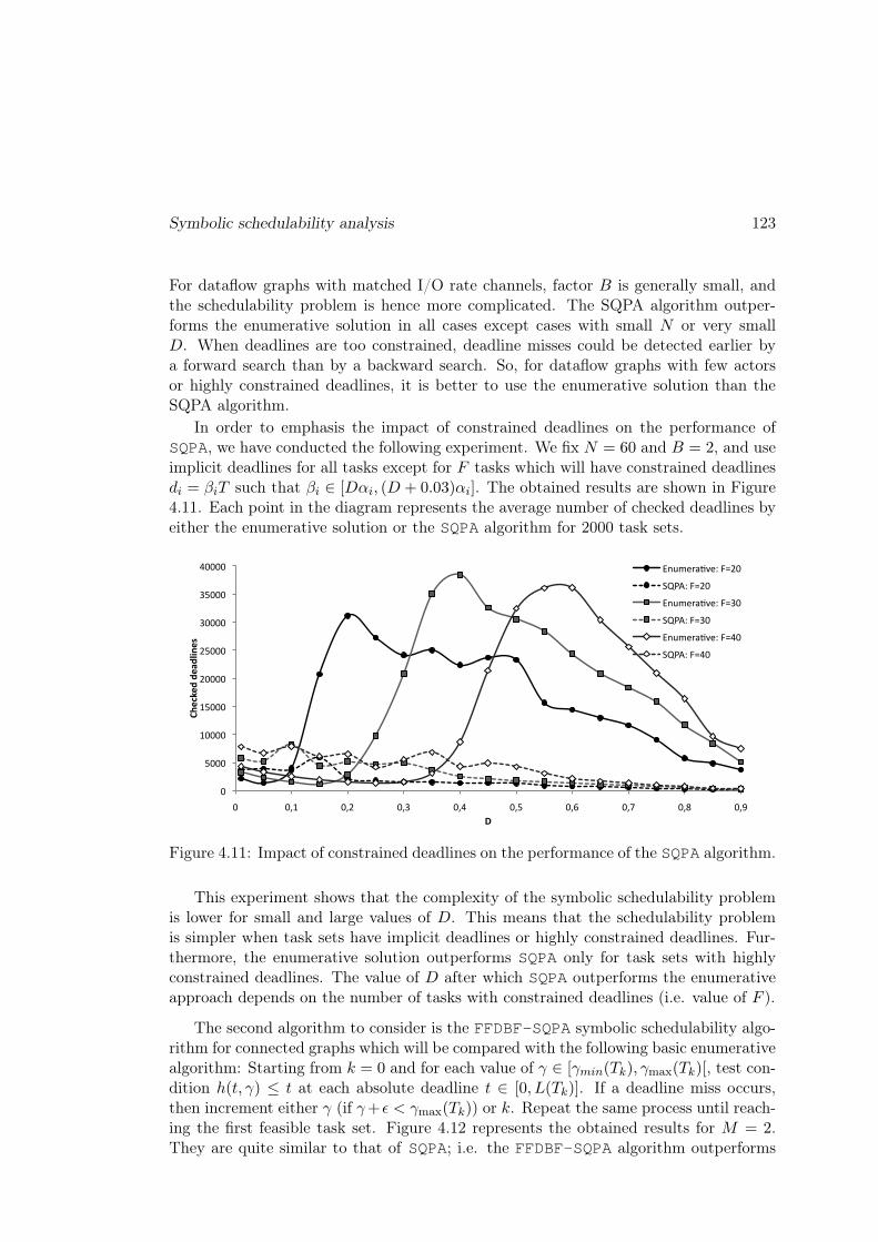
Symbolic schedulability analysis 123
For dataflow graphs with matched I/O rate channels, factor B is generally small, andthe schedulability problem is hence more complicated. The SQPA algorithm outper-forms the enumerative solution in all cases except cases with small N or very smallD. When deadlines are too constrained, deadline misses could be detected earlier bya forward search than by a backward search. So, for dataflow graphs with few actorsor highly constrained deadlines, it is better to use the enumerative solution than theSQPA algorithm.
In order to emphasis the impact of constrained deadlines on the performance ofSQPA, we have conducted the following experiment. We fix N = 60 and B = 2, and useimplicit deadlines for all tasks except for F tasks which will have constrained deadlinesdi = βiT such that βi ∈ [Dαi, (D + 0.03)αi]. The obtained results are shown in Figure4.11. Each point in the diagram represents the average number of checked deadlines byeither the enumerative solution or the SQPA algorithm for 2000 task sets.
!"
#!!!"
$!!!!"
$#!!!"
%!!!!"
%#!!!"
&!!!!"
&#!!!"
'!!!!"
!" !($" !(%" !(&" !('" !(#" !()" !(*" !(+" !(,"
!"#$%#&'&#
(&)*+
#,'
-'
-./01234516"78%!"
9:;<6"78%!"
-./01234516"78&!"
9:;<6"78&!"
-./01234516"78'!"
9:;<6"78'!"
Figure 4.11: Impact of constrained deadlines on the performance of the SQPA algorithm.
This experiment shows that the complexity of the symbolic schedulability problemis lower for small and large values of D. This means that the schedulability problemis simpler when task sets have implicit deadlines or highly constrained deadlines. Fur-thermore, the enumerative solution outperforms SQPA only for task sets with highlyconstrained deadlines. The value of D after which SQPA outperforms the enumerativeapproach depends on the number of tasks with constrained deadlines (i.e. value of F ).
The second algorithm to consider is the FFDBF-SQPA symbolic schedulability algo-rithm for connected graphs which will be compared with the following basic enumerativealgorithm: Starting from k = 0 and for each value of γ ∈ [γmin(Tk), γmax(Tk)[, test con-dition h(t, γ) ≤ t at each absolute deadline t ∈ [0, L(Tk)]. If a deadline miss occurs,then increment either γ (if γ+ǫ < γmax(Tk)) or k. Repeat the same process until reach-ing the first feasible task set. Figure 4.12 represents the obtained results for M = 2.They are quite similar to that of SQPA; i.e. the FFDBF-SQPA algorithm outperforms

124 Experimental validation
the enumerative approach for non-small values of N and D. We note that in case ofFFDBF-SQPA, parameter D has more impact than factor B on the complexity of theproblem.
!"
#"
$!"
$#"
%!"
%#"
&!"
&#"
#" $#" %#" &#" '#" ##" (#" )#" &#" +#"
!"#$%#&'&#
(&)*+
#,'
-*.#'/0'1(,%',#1,'
,-%."/-!0)."1-&!0$'" ,-&."/-!0%."1-$++0&"
,-$)#."/-!0(."1-'0+" ,-&!."/-!0!$."1-+(0%'"
Figure 4.12: Performance of the FFDBF-SQPA algorithm.
Let us now measure the impact of the number of processors on the performance ofthe FFDBF-SQPA algorithm. So, we fix N = 100 and B = 2 while we vary M from2 to 20. The obtained results for two values of D (D = 0.6 and D = 0.2) are shownin Figure 4.13. Each point in the diagram represents the average number of checkeddeadlines by either the enumerative solution or the FFDBF-SQPA algorithm for 2000task sets. Firstly, you may notice the drastic impact of parameter D on the numberof checked points (by comparing curves Enumerative: D=0.6 and Enumerative: D=0.2).This impact is almost constant over the entire range of number of processors (a factorof 1.6). Regarding the impact of parameter M on the performance of FFDBF-SQPA, wefound that the benefit (i.e. reduction of complexity in comparison with the enumerative
!"
#!!!"
$!!!"
%!!!"
&!!!"
'!!!"
(!!!"
)!!!"
$" &" (" *" #!" #$" #&" #(" #*" $!"
!"#$%#&'&#
(&)*+
#,'
-./0#1'23'412$#,,21,'
+,-./0123/4"56!7("88598:;<=>4"56!7("+,-./0123/4"56!7$"88598:;<=>4"56!7$"
Figure 4.13: Impact of the number of processors on the performance of the FFDBF-SQPAalgorithm.

Symbolic schedulability analysis 125
solution) is almost constant for D = 0.6 and monotonic for D = 0.2. Furthermore, thecomplexity of the schedulability problem decreases when adding more processors.
The last algorithm to consider is the DF-B&B SQPA algorithm (i.e. SQPA for dis-connected graphs). We generate disconnected graphs with L = 2, Bj ∈ [10, 20], andT uj = 10⌈σj⌉. The enumerative solution proceeds as follows: starting from T = T l,
test condition h(t) ≤ t at each absolute deadline in [0, L(T )]. If there is a miss, thenput T = getNext() and repeat the same process until reaching the first feasible taskset. Function getNext() returns the next unexplored point in the T -space that resultsin the maximum utilization. The huge overhead of this method is not considered inthe comparison. Figure 4.14 shows the obtained results. Each point in the diagram isthe ratio of the average number of checked deadlines by the enumerative solution (for100 task sets) to the average number of checked deadlines by DF-B&B SQPA. For eachconfiguration, we denote by E the average number of checked points per task (obtainedby the enumerative solution) to indicate the complexity of the problem. Again, thesymbolic schedulability problem is more complex for large values of D. Furthermore,DF-B&B SQPA outperforms the enumerative solution for non-small values of N and D.
!"
%!"
'!"
(!"
&!"
$!!"
$%!"
(" $%" $&" %'" &!" &(" '%" '&" #'" (!" ((" )%" )&" &'" +!" +("
!"#!$#%&%#
'%()*
#+&
,)-#&./&0'+$&+#0+&
,-%."/-!0)."1-&!+*(.*')$+"
,-%."/-!0&."1-$$($%.)*#&'"
Figure 4.14: Performance of the DF-B&B SQPA algorithm.
4.2.2 Fixed-priority scheduling
Let us first consider the SRTA algorithm (i.e. connected dataflow graphs) with fixedpriorities (i.e. a unique priority region). We assume that tasks have priorities in thesame order in which they were randomly generated. The obtained results are shown inFigure 4.15 where each point represents the ratio of the average number of computedresponse times by the enumerative solution (for 2000 task sets) to the average number ofcomputed response times by SRTA. The enumerative algorithm consists in the followingsteps: starting from k = 0, perform RTA. If the task set is not feasible, then incrementk and repeat the same process until reaching the first feasible task set. The differencebetween the performance of SRTA and the performance of the basic algorithm is quitehuge and unexpected. For instance, for N = 100, B = 2, and D = 0.7, SRTA requires

126 Experimental validation
the computation of only 13 response times while the basic approach requires to computemore than 224426 response times. In fact, for the four configurations, SRTA requires tocompute at most 13 response times.
!"
#!!!"
$!!!!"
$#!!!"
%!!!!"
%#!!!"
#" $#" %#" &#" '#" ##" (#" )#" *#" +#"
!"#$%
&'()*'+$",
+')-#'+)
./0')"1)&2+3)+'&+)
,-%."/-!0)."1-$#()0'%" ,-&."/-!0%."1-%$')0$("
,-$)#."/-!0(."1-%%0%#" ,-&!."/-!0!$."1-$!&'0("
Figure 4.15: Performance of the SRTA algorithm.
The second schedulability algorithm to address is the DF-B&B SRTA algorithm (i.e.SRTA for disconnected graphs). We follow the same approach, described in the previoussection, to generate disconnected graphs with L = 2, B ∈ [10, 20], and Tj = 100⌈σj⌉.The enumerative solution proceeds as follows: starting from T = T l, perform RTA. Ifthere is a deadline miss, then put T = getNext() and repeat the same process untilreaching the first feasible task set. Figure 4.16 presents the obtained results where eachpoint in the diagram represents the ratio of the average number of computed responsetimes by the enumerative solution (for 50 task sets) to the average number of computedresponse times by DF-B&B SRTA. The performance of the DF-B&B SRTA algorithm isnot as good as expected, especially in comparison with the performance of the SRTA
algorithm. Thus, the problem should be further researched to identify better algorithms.
!"
#"
$!"
$#"
%!"
%#"
&!"
&#"
'!"
'#"
#!"
(" $%" $)" %'" &!" &(" '%" ')" #'" (!" ((" *%" *)"
!"#$%
&'()*'+$",
+')-#'+)
./0')"1)&2+3)+'&+)
+,%-".,!/*-"0,%')!#/%)"
+,%-".,!/&-"0,(!(!!/%"
Figure 4.16: Performance of the DF-B&B SRTA algorithm.

Application: Design of SCJ/L1 systems 127
4.3 Application: Design of SCJ/L1 systems
In recent years, there has been a growing interest in using Java for safety-critical systemssuch as flight control systems, railway signaling systems, robotic surgery machines, etc.The high productivity of Java compared to low-level languages is one among multiplereasons that encourage efforts to develop Java environments for both high-end and low-end embedded devices. FijiVM, JamaicaVM, PERC, PERC Pico, KESO, and Muviumare examples of such environments. Much ongoing effort, mainly made by the JSR-302expert group, is focused on developing the Safety-Critical Java (SCJ) specification [104].SCJ is a subset of Java augmented by the Real-Time Specification for Java (RTSJ) [90]and intended to develop applications that are amenable to certification under safetycritical standards (such as DO-178B, Level A).
To better meet domain-specific safety requirements, the SCJ specification definesthree levels of compliance (Levels 0, 1, and 2), each with a different model of concurrency,each aiming at applications of specific criticality. By the time of writing, there are fewand incomplete implementations (only levels 0 and 1) of SCJ specification; for instanceoSCJ [156] implemented on top of FijiVM [155], SCJ implemented on top of HVM [169],and the prototype implementation of SCJ on the Java processor JOP [162]. We havechosen Level 1 because it is less restricted than Level 0 and more analyzable than Level2 not yet implemented. Indeed, SCJ/L0 supports only periodic handlers scheduledby a cyclic executive on a single processor; while SCJ/L2 has a much complicatedconcurrency model with nested missions, no-heap real-time threads, inter-processor jobmigration, self-suspension, etc.
In this section, we will focus on the concurrency model of SCJ/L1 rather than itsmemory model. SCJ/L1 relies entirely on periodic and aperiodic event handling. Eachhandler has its own server thread; this is however inconsistent with RTSJ in whicha many-to-one relationship between handlers and servers is allowed [193]. Handlerscommunicate through shared memory; concurrency therefore becomes an issue as theprogrammer has to deal with data races, priority inversion, and deadlocks. In orderto avoid data races, lock-based synchronization protocols are required though they areextremely complex and require pessimistic schedulability analyses.
Our objective is to propose a dataflow design model of SCJ/L1 applications (as anextension to the affine dataflow model) in which handlers communicate only throughlock-free channels. Using dataflow diagrams to model real-time Java applications isnot a new idea. Indeed, dataflow models of computation have been used in many real-time Java programming models such as Eventrons [170], Reflexes [171], Exotasks [6],StreamFlex [172], and Flexotasks [5]. The main goal of those restricted subsets of Java isto achieve lower latencies than what can be achieved by the real-time garbage collector.They attest the software engineering benefits of the dataflow model by offering somemodel-driven development capabilities such as automatic code generation. Some ofthem also provide type systems to ensure memory isolation; i.e. tasks can communicateonly through specific mechanisms such as buffers and transactional memory. The abovementioned issues have been already partially solved by the SCJ memory model [55] orthe SCJ annotation checker [186]. Those dataflow programming models lack however the

128 Experimental validation
necessary tools for computing buffer sizes and priority-driven scheduling parameters.
4.3.1 Concurrency model of SCJ/L1
A SCJ/L1 application consists of a set of missions executed in sequence; nested missionsare hence not allowed. The infrastructure MissionSequencer thread is responsibleof creating and terminating missions, one after another. As depicted in Figure 4.17, amission starts in an initialization phase during which schedulable objects (periodic andaperiodic event handlers) are created. Thus, the number and scheduling parameters(i.e. periods, phases, deadlines, priorities, etc.) of handlers are known at compile-time.Handlers are released during the mission execution phase such that periodic handlerreleases are time-triggered while aperiodic handler releases are event-triggered. SCJ/L1specification does not support sporadic releases; therefore, aperiodic handlers can haveonly soft deadlines since the assumptions necessary to check their schedulability arenot part of the profile. Each handler overrides the handleAsyncEvent() method toprovide the computational logic executed when the handler is released. This is somehowsimilar to firing functions of actors in dataflow graphs and hence justifies our choice of a dataflowdesign model.
Application.setup()
Mission.initialize() Execution Mission.cleanup()
Application.teardown()
MissionSequencer.getNextMission()
Figure 4.17: SCJ mission life cycle.
Periodic and aperiodic handlers are bound asynchronous event handlers; i.e. eachhandler is permanently bound to a single implementation thread. Each handler hasa fixed priority; and the set of handlers is executed in parallel with a full preemptivepriority-based scheduler. Handlers cannot self suspend and access to shared data iscontrolled by synchronized methods and statement blocks to avoid race conditions.The scheduler must implement the priority ceiling emulation protocol.
Scheduling aperiodic tasks based on their priorities may cause some lower priorityhard tasks to miss their deadlines. Among the proposed solutions, aperiodic servers havebeen devised to improve the average response time of soft aperiodic tasks; examplesof such techniques are: polling servers, deferrable servers, sporadic servers, priorityexchange servers, etc. See Section 1.4.3 for more details. The SCJ specification is silentabout using such approaches to execute aperiodic handlers although sporadic servers,for instance, are now supported by the POSIX standard P1003.1d. In the sequel, wepropose to use sporadic servers; nevertheless, the presented technique can be easilyadapted to consider polling servers or deferrable servers.
SCJ/L1 also supports multiprocessor implementations which require full partitionedscheduling (through the notion of Affinity Sets). Each handler can execute on a fixedprocessor with no migration (i.e. a partitioned FP scheduling).

Application: Design of SCJ/L1 systems 129
4.3.2 Dataflow design model
Since missions are independent, each mission will be separately designed as a dataflowgraph; while the mission sequencer can be modeled by a finite state machine. So,an actor in a dataflow graph represents a SCJ handler. The necessary user-providedinformation about a mission are illustrated in Figure 4.18.
Circle nodes represent periodic actors. The user must provide the worst-case exe-cution time of each actor and the production and consumption rates of FIFO channels(solid arrows between periodic actors). Those rates can be just a safe abstraction ofthe actual production and consumption rates that can be obtained by some static codeanalysis. A FIFO channel e will be simply implemented as a cyclic array E with a fixedsize s such that the instruction e.set(v) is implemented as {E[i]=v;i=(i+1)%s;}where i is a local index in the producer. Calls for the get() method are implementedin a similar way. The overflow and underflow analyses will ensure that there will beno need for synchronization protocols to access the arrays. Two non-communicatingperiodic actors can be linked together via an affine relation to relate their speeds toeach other. Actors p3 and p2 are (2, 0, 1)-affine-related which means that actor p2 istwice as fast as actor p3.
Figure 4.18: An ultimately cyclo-static dataflow graph with aperiodic actors.
Rectangle nodes represent aperiodic handlers. Actor p4 is an aperiodic handlerbound to a sporadic server thread which has a capacity equal to 75 and a replenishmentperiod equal to 540. Parameters of servers that minimize the average response times aregenerally obtained by simulation. Some selection criteria have been proposed in [22].Since there can be multiple servers in the system, a capacity sharing protocol like theone described in [23] may increase the responsiveness of aperiodic tasks.
Besides having unknown (or extremely large) worst-case execution times, aperiodictasks have unknown interarrival time of requests. Therefore, an aperiodic task cannotcommunicate with other tasks via simple FIFO channels. Indeed, these communicationsmay be unbounded or empty and hence block the other tasks for an indeterminate time.In our design model, an aperiodic task communicates with other (periodic or aperiodic)tasks through Cyclical Asynchronous Buffers (CAB) [61]. CABs offer bounded non-blocking communications. Tokens in a CAB are maintained until they are over-writtenby the producer. Hence, some produced tokens are lost if the producer is faster than theconsumer; and the consumer may read the same tokens several times if it is faster thanthe producer. This is not a problem in many control applications, where tasks requirefresh data rather than the complete stream. CABs were used in HARTIK system [52]and SimpleRTK. Sample-and-hold communication mechanisms are used in many designmodels; for instance in the Architecture Analysis and Design Language (AADL) [161]

130 Experimental validation
and the Prelude compiler [149]. Based on the parameters of the aperiodic servers boundto the aperiodic tasks, it is possible to compute the average sizes of CABs.
The user may provide further optional information: (1) Lower bounds and upperbounds on periods. (2) Constrained deadlines of tasks as fractions (less than one) ofperiods; otherwise deadlines are assumed to be implicit. (3) The number of identi-cal processors for multiprocessor implementations; otherwise uniprocessor scheduling isconsidered. (4) Buffer sizes and number of initial tokens in channels.
Implementation
The presented dataflow design model comes with a development tool integrated in theEclipse IDE for easing the development of SCJ/L1 applications and enforcing the restric-tions imposed by the design model. It consists of a GMF editor where applications aredesigned graphically and timing and buffering parameters can be synthesized. Indeed,affine scheduling is first applied on the dataflow subgraph that consists only of periodicactors. Then, symbolic FP schedulability analysis considers both periodic and aperiodicactors. Thanks to equations such as Equation 1.14 (p. 45), SRTA can be easily extendedto consider also sporadic servers. Through a model-to-text transformation, using Ac-celeo, the SCJ code for missions, interfaces of handlers, and the mission sequencer isautomatically generated in addition to the annotations needed by the memory checker.
Figure 4.19: Graphical editor for SCJ/L1 applications design.
Channels are implemented as cyclic arrays or CABs and a fixed amount of memoryis hence reused to store the infinite streams of tokens. Channels are instantiated inthe mission memory since event handlers execute in private memory areas and cancommunicate only through mission memory (or the immortal memory). For instance,

Conclusion 131
when a handler reads a token from a channel, it simply copies the token from the missionmemory to its private memory.
The user must provide the SCJ code of all the handleAsyncEvent() methods.We have integrated the SCJ memory checker in our tool so that potential danglingpointers can be highlighted at compile-time. A dangling pointer is a reference froman object allocated in a long-lived memory area (e.g. the immortal memory which isdestroyed only at the end of the application) to an object allocated in a short-livedmemory area (e.g. the private memory of a handler which is destroyed each time itsfiring function completes).
4.4 Conclusion
In this chapter, we have performed several experiments on either real-life benchmarks orrandomly generated graphs and task sets. We have compared our tool with the DARTS
tool and shown that our symbolic schedulability tests are generally more accurate.We have also shown the improvement on buffering requirements that can be achievedby the priority assignment and deadlines adjustment techniques. Furthermore, we haveshown that our symbolic schedulability tests are much faster than the basic enumerativesolutions in most cases. Finally, we have briefly present how to use the affine schedulingtechnique to automatically generate SCJ/L1 applications from a dataflow specification.

132 Experimental validation

Conclusion
The design of real-time safety-critical applications is getting more and more complexdue to the ever-increasing functional and nonfunctional requirements. This calls for newdesign flows that solve the specification, validation, and synthesis problems. Formalmodels must be used to describe the system, then formal analysis techniques explorethe design space to assess feasibility and find the optimal design before the costlyimplementation phase. Finally, automatic synthesis techniques should be used as muchas possible to generate correct by construction implementations.
Any design flow must ensure two key properties of a real-time safety-critical sys-tem, namely, functional determinism and temporal predictability. Dataflow models ofcomputation (e.g. SDF, CSDF, etc.) are widely used to design stream-based embeddedsystems thanks to their inherent functional determinism. Since the introduction of theSDF model, a considerable effort has been made to solve the static-periodic schedulingproblem; i.e. the construction of periodic infinite sequences of firings of actors thatresult in bounded, live, and complete executions. Ensuring boundedness and livenessis the essence of the proposed algorithms in addition to optimizing some nonfunctionalperformance metrics (e.g. buffer minimization, throughput maximization, code sizeminimization, etc.). We tried in Chapter 1 to present a survey of dataflow modelsof computation together with the existing algorithms for static-periodic scheduling of(C|H)SDF graphs.
Nowadays real-time embedded systems are so complex that real-time operating sys-tems are used to manage hardware resources and host real-time tasks. Most of real-timeoperating systems rely on priority-driven scheduling algorithms (e.g. RM, EDF, etc.)instead of static-periodic schedules (also called cyclic executives) because of the inflex-ibility and difficult maintainability of cyclic executives. Real-time scheduling theoryprovides the necessary schedulability tests to verify that all real-time tasks will meettheir deadlines even in the worst-case scenario. In Chapter 1, we have presented someof the schedulability tests regarding EDF and FP scheduling for uniprocessor and mul-tiprocessor architectures. The underlying model of computation was the periodic taskmodel which consists of a set of independent and concurrent real-time tasks.
This thesis has addressed the problem of implementing a dataflow specification asa set of independent real-time tasks to be executed on a system equipped with a real-time operating system [45, 43, 44]. This problem consists in mapping each actor inthe dataflow graph to a periodic real-time task with appropriate scheduling parameters(i.e. period, first start time, priority, processor allocation, etc.). Certainly, properties
133

134 Conclusion
such as boundedness and liveness must also be considered. Since reads and writesin the periodic task model are non-blocking operations, we have talked more aboutoverflow and underflow exceptions over communication channels. Real-time schedulingof dataflow graphs is not a trivial problem. We have solved it in two steps: abstractscheduling (Chapter 2) and symbolic schedulability analysis (Chapter 3). Let us recallthe contributions made at each step:
Abstract scheduling
1. Activation-related schedules are presented, together with the necessary conditionsfor boundedness, liveness, and consistency, as a general framework to describe schedulesof static dataflow graphs.
2. Affine relations are used to describe strictly periodic schedules. The objective ofthe ILP formalization of the problem was to minimize the buffering requirements in amachine-independent way.
3. We have also presented UCSDF (a generalization of CSDF), FRStream (a syn-chronous operational semantics for UCSDF graphs), multichannels, and how channelscan share the same storage space.
Symbolic real-time schedulability analysis
1. We have created a new application field for parametric schedulability theory.
2. We have presented many symbolic EDF schedulability analyses (e.g. SQPA, DF-B&BSQPA, FFDBF-SQPA, BF-EDF, etc.) that aim at maximizing the processor utilizationfactor. We have shown that our schedulability tests have a lower complexity than thebasic enumerative solutions. We have also presented a deadline adjustment technique(to encode scheduling precedences) that aims at minimizing the buffering requirements.
3. Finally, many symbolic FP schedulability tests are presented (e.g. SRTA, DF-B&BSRTA, etc.). We also presented some priority assignment strategies that aim at ei-ther minimizing the buffering requirements, maximizing the throughput, or finding acompromised solution.
In Chapter 4, we have shown that our tool (the ADFG tool) outperforms the onlyexisting tool for real-time scheduling of dataflow graphs (the DARTS tool). We have alsobriefly presented our graphical editor for automatic synthesis of SCJ Level 1 applicationsfrom UCDF graph specifications. Certainly, the synthesis flow relies on affine schedulingand symbolic FP schedulability analysis to transform the dataflow specification to a setof independent periodic SCJ handlers.
Perspectives
This thesis is one among the fewest studies that have addressed the real-time schedul-ing problem of dataflow graphs. However, it offers by no means complete or optimal
Conclusion 135
solutions. Several points need to be researched further; for example:
1. Expressive dataflow models: Though the abstract scheduling approach (Section 2.2)has been presented for arbitrary rate functions and activation relations, we have onlyimplemented a specific case where infinite integer sequences (used either to describeactivation relations or rate functions) were ultimately periodic. It will be very interestingto find more expressive classes of integer sequences that could be used as rate functionsand yet define an analyzable model.
2. Symbolic schedulability analysis: We have focused more on symbolic schedulabilityanalysis of connected graphs. The design parameter space could be further relaxedto consider: disconnected graphs, arbitrary deadlines, more priority assignment strate-gies, etc. More performance metrics should also be addressed as energy consumptionminimization. We believe that this research field is very large, complex, and not yetexplored.
3. Actor clustering: In the presented scheduling approach, each actor is mapped toa periodic real-time task. However, a large set of real-time tasks could result in anoticeable run-time overhead (due to context switching, scheduling decisions, etc.). Itmay be hence reasonable to map many actors to a single real-time task so that eachtask consists in a static schedule of its actors.
4. Design of SCJ\L1 applications: To enhance functional determinism, we would like todevelop an ownership type system, as the one presented in Reflexes, to ensure firstlythat actors are strongly isolated; i.e. objects allocated within an actor are encapsulatedunless they are full-immutable. This requirement ensures that the state of an actorcannot be altered by other actors. Typing rules such as “a non-private field must beeither a final primitive or a final reference to a full-immutable object” and “non-privatemethods of an actor do not change its state or leak references to mutable objects” mustbe checked statically. Besides isolation of actors, the type system must ensure thatactors can communicate only through buffers. Hence, “shared objects in the immortalor mission memory areas must be either final primitives or final references to full-immutable objects”. Our future work will also consider to develop a static analysisthat infers safe production and consumption rates from the user-provided SCJ code offiring functions and to connect our tool to existing worst-case execution time estimationtools.

136 Conclusion

Bibliography
[1] M. Adé, R. Lauwereins, and J. A. Peperstraete. Data memory minimization forsynchronous data flow graphs emulated on DSP-FPGA targets. In Proceedings ofthe 34th Annual Design Automation Conference, pages 64–69, 1997.
[2] B. Anderson, S. Baruah, and J. Jonsson. Static-priority scheduling on multipro-cessors. In Proceedings of the 22nd IEEE Real-Time Systems Symposium, pages 193–202,2001.
[3] N. Audsley, A. Burns, M. Richardson, K. Tindell, and A. J. Wellings. Applyingnew scheduling theory to static priority pre-emptive scheduling. Software Engineer-ing Journal, 8:284–292, 1993.
[4] N. C. Audsley. On priority assignment in fixed priority scheduling. Inf. Process.Lett., 79(1):39–44, 2001.
[5] J. Auerbach, D. F. Bacon, R. Guerraoui, J. H. Spring, and J. Vitek. Flexible taskgraphs: a unified restricted thread programming model for Java. SIGPLAN Not.,43(7):1–11, 2008.
[6] J. Auerbach, D. F. Bacon, D. T. Iercan, C. M. Kirsch, V. Rajan, H. Roeck,and R. Trummer. Java takes flight: time-portable real-time programming withExotasks. SIGPLAN Not., 42(7):51–62, 2007.
[7] F. Baccelli, G. Cohen, G. J. Oldsder, and J.-P. Quadrat. Synchronization andlinearity: an algebra for discrete event systems. Wiley, 1992.
[8] T. P. Baker. A comparison of global and partitioned EDF schedulability testsfor multiprocessors. In Proceedings of the International Conference on Real-Time andNetwork Systems, pages 119–130, 2006.
[9] M. Bamakhrama and T. Stefanov. Hard-real-time scheduling of data-dependenttasks in embedded streaming applications. In Proceedings of the 9th ACM Interna-tional Conference on Embedded Software, pages 195–204, 2011.
[10] M. A. Bamakhrama and T. Stefanov. Managing latency in embedded streamingapplications under hard-real-time scheduling. In Proceedings of the 8th IEEE/ACM/I-FIP International Conference on Hardware/Software Codesign and System Synthesis,pages 83–92, 2012.
[11] S. Baruah, V. Bonifaci, A. Marchetti-Spaccamela, and S. Stiller. Implementa-tion of speedup-optimal global EDF schedulability test. In Proceedings of the 21st
137

138 Bibliography
Euromicro Conference on Real-Time Systems, pages 259–268, 2009.
[12] S. Baruah and N. Fisher. The partitioned multiprocessor scheduling of sporadictask systems. In Proceedings of the 26th IEEE International Real-Time Systems Sympo-sium, pages 321–329, 2005.
[13] S. Baruah and N. Fisher. The partitioned multiprocessor scheduling of deadline-constrained sporadic task systems. IEEE Trans. Comput., 55(7):918–923, 2006.
[14] S. K. Baruah, R. R. Howell, and L. E. Rosier. Feasibility problems for recurringtasks on one processor. Theor. Comput. Sci., 118(1):3–20, 1993.
[15] S. K. Baruah, A. K. Mok, and L. E. Rosier. Preemptively scheduling hard-real-time sporadic tasks on one processor. In Proceedings of the 11th Real-Time SystemsSymposium, pages 182–190, 1990.
[16] T. Basten and J. Hoogerbrugg. Efficient execution of process networks. In Com-municating Process Architectures, pages 1–14, 2001.
[17] S. S. Battacharyya, E. A. Lee, and P. K. Murthy. Software synthesis from dataflowgraphs. Kluwer Academic Publishers, Norwell, MA, USA, 1996.
[18] M. Benazouz, O. Marchetti, A. M. Kordon, and P. Urard. A new approach for min-imizing buffer capacities with throughput constraint for embedded system design.In Proceedings of the 8th ACS/IEEE Conference on Computer Systems and Applications,pages 1–8, 2010.
[19] A. Benveniste, B. Caillaud, and P. Le Guernic. From synchrony to asynchrony.In Proceedings of the 10th International Conference on Concurrency Theory, pages 162–177, 1999.
[20] A. Benveniste, B. Caillaud, and P. Le Guernic. Compositionality in dataflowsynchronous languages: specification & distributed code generation. Informationand Computation, 163(1):125–171, 2000.
[21] A. Benveniste, P. Caspi, S. A. Edwards, N. Halbwachs, P. Le Guernic, andR. de Simone. The synchronous languages 12 years later. Proceedings of the IEEE,91(1):64–83, 2003.
[22] G. Bernat and A. Burns. New results on fixed priority aperiodic servers. InProceedings of the 20th IEEE Real-Time Systems Symposium, pages 68–78, 1999.
[23] G. Bernat and A. Burns. Multiple servers and capacity sharing for implementingflexible scheduling. Real-Time Syst., 22(1/2):49–75, 2002.
[24] G. Berry. The foundations of Esterel. In Proof, language, and interaction, pages425–454. MIT Press, Cambridge, MA, USA, 2000.
[25] M. Bertogna and S. Baruah. Tests for global EDF schedulability analysis. J. Syst.Archit., 57(5):487–497, 2011.
[26] M. Bertogna and M. Cirinei. Response-time analysis for globally scheduled sym-metric multiprocessor platforms. In Proceedings of the 28th IEEE International Real-Time Systems Symposium, pages 149–160, 2007.
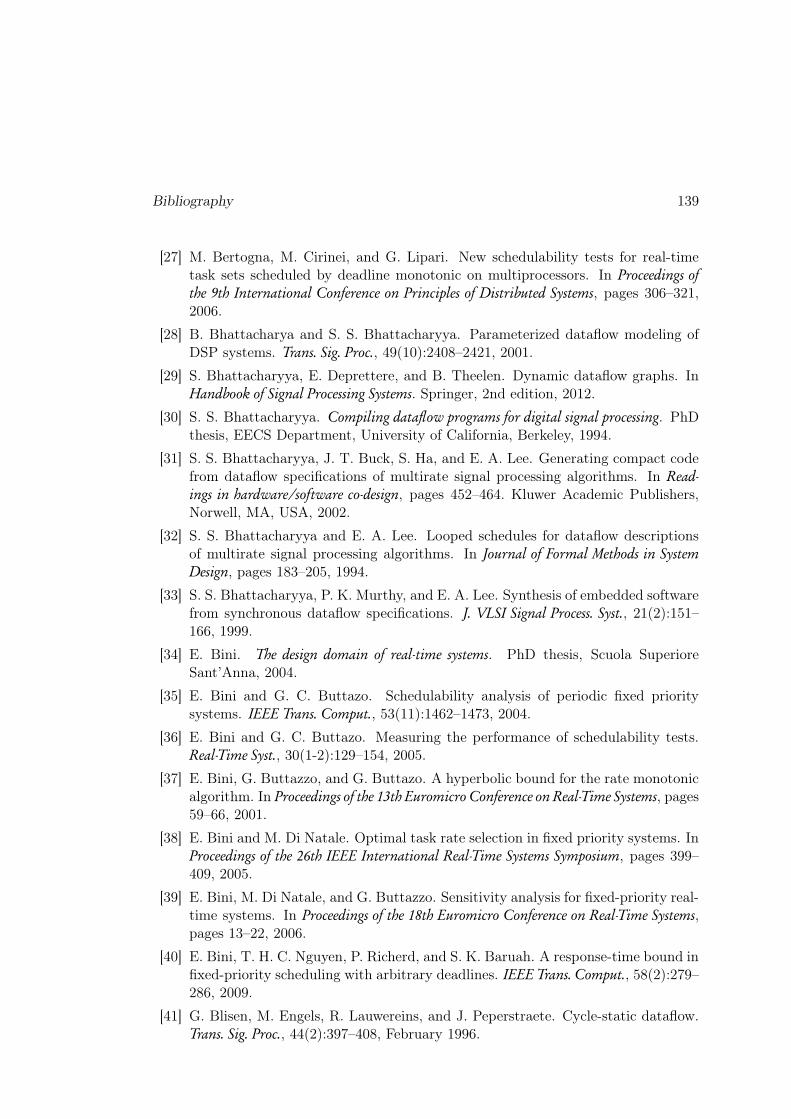
Bibliography 139
[27] M. Bertogna, M. Cirinei, and G. Lipari. New schedulability tests for real-timetask sets scheduled by deadline monotonic on multiprocessors. In Proceedings ofthe 9th International Conference on Principles of Distributed Systems, pages 306–321,2006.
[28] B. Bhattacharya and S. S. Bhattacharyya. Parameterized dataflow modeling ofDSP systems. Trans. Sig. Proc., 49(10):2408–2421, 2001.
[29] S. Bhattacharyya, E. Deprettere, and B. Theelen. Dynamic dataflow graphs. InHandbook of Signal Processing Systems. Springer, 2nd edition, 2012.
[30] S. S. Bhattacharyya. Compiling dataflow programs for digital signal processing. PhDthesis, EECS Department, University of California, Berkeley, 1994.
[31] S. S. Bhattacharyya, J. T. Buck, S. Ha, and E. A. Lee. Generating compact codefrom dataflow specifications of multirate signal processing algorithms. In Read-ings in hardware/software co-design, pages 452–464. Kluwer Academic Publishers,Norwell, MA, USA, 2002.
[32] S. S. Bhattacharyya and E. A. Lee. Looped schedules for dataflow descriptionsof multirate signal processing algorithms. In Journal of Formal Methods in SystemDesign, pages 183–205, 1994.
[33] S. S. Bhattacharyya, P. K. Murthy, and E. A. Lee. Synthesis of embedded softwarefrom synchronous dataflow specifications. J. VLSI Signal Process. Syst., 21(2):151–166, 1999.
[34] E. Bini. The design domain of real-time systems. PhD thesis, Scuola SuperioreSant’Anna, 2004.
[35] E. Bini and G. C. Buttazo. Schedulability analysis of periodic fixed prioritysystems. IEEE Trans. Comput., 53(11):1462–1473, 2004.
[36] E. Bini and G. C. Buttazo. Measuring the performance of schedulability tests.Real-Time Syst., 30(1-2):129–154, 2005.
[37] E. Bini, G. Buttazzo, and G. Buttazo. A hyperbolic bound for the rate monotonicalgorithm. In Proceedings of the 13th Euromicro Conference on Real-Time Systems, pages59–66, 2001.
[38] E. Bini and M. Di Natale. Optimal task rate selection in fixed priority systems. InProceedings of the 26th IEEE International Real-Time Systems Symposium, pages 399–409, 2005.
[39] E. Bini, M. Di Natale, and G. Buttazzo. Sensitivity analysis for fixed-priority real-time systems. In Proceedings of the 18th Euromicro Conference on Real-Time Systems,pages 13–22, 2006.
[40] E. Bini, T. H. C. Nguyen, P. Richerd, and S. K. Baruah. A response-time bound infixed-priority scheduling with arbitrary deadlines. IEEE Trans. Comput., 58(2):279–286, 2009.
[41] G. Blisen, M. Engels, R. Lauwereins, and J. Peperstraete. Cycle-static dataflow.Trans. Sig. Proc., 44(2):397–408, February 1996.

140 Bibliography
[42] A. Bonfietti, M. Lombardi, M. Milano, and L. Benini. Throughput constraintfor synchronous data flow graphs. In Proceedings of the 6th International Conferenceon Integration of AI and OR Techniques in Constraint Programming for CombinatorialOptimization Problems, pages 26–40, 2009.
[43] A. Bouakaz and J.-P. Talpin. Buffer minimization in earliest-deadline first schedul-ing of dataflow graphs. SIGPLAN Not., 48(5):133–142, 2013.
[44] A. Bouakaz and J.-P. Talpin. Design of safety-critical Java level 1 applicationsusing affine abstract clocks. In Proceedings of the 16th International Workshop onSoftware and Compilers for Embedded Systems, pages 58–67, 2013.
[45] A. Bouakaz, J.-P. Talpin, and J. Vitek. Affine data-flow graphs for the synthesisof hard real-time applications. In Proceedings of the 12th International Conference onApplication of Concurrency to System Design, pages 183–192, 2012.
[46] L. C. Briand and D. M. Roy. Meeting deadlines in hard real-time systems : the ratemonotonic approach. IEEE, 1999.
[47] J. D. Brock and W. B. Ackerman. Scenarios: a model of non-determinate compu-tation. In Proceedings of the International Colloquim on Formalization of ProgrammingConcepts, pages 252–259, 1981.
[48] J. T. Buck. Scheduling dynamic dataflow graphs with bounded memory using the tokenflow model. PhD thesis, EECS Department, University of California, Berkeley,1993.
[49] J. T. Buck. Static scheduling and code generation from dynamic dataflow graphswith integer-valued control systems. In Proceedings of the 28th Annual AsilomarConference on Signals, Systems, and Computers, pages 508–513, 1994.
[50] A. Burns and S. Baruah. Sustainability in real-time scheduling. Journal of ComputerScience and Engineering, 2(1):74–97, 2008.
[51] G. C. Buttazo. Hard real-time computing systems: predictable scheduling algorithms andapplications. Kluwer Academic Publishers, Norwell, MA, USA, 1997.
[52] G. Buttazzo and M. Di Natale. HARTIK: a hard real-time kernel for programmingrobot tasks with explicit time constraints and guaranteed execution. In Proceedingsof IEEE International Conference on Robotics and Automation, pages 404–409, 1993.
[53] P. Caspi, C. Mazuet, and N. R. Paligot. About the design of distributed controlsystems: the quasi-synchronous approach. In Proceedings of the 20th InternationalConference on Computer Safety, Reliability and Security, pages 215–226, 2001.
[54] P. Caspi and M. Pouzet. Synchronous Kahn networks. SIGPLAN NOT., 31(6):226–238, 1996.
[55] A. Cavalcanti, A. Wellings, and J. Woodcock. The safety-critical Java memorymodel: a formal account. In Proceedings of the 17th International Conference onFormal Methods, pages 246–261, 2011.
[56] S. Chakraborty, S. Kunzli, and L. Thiele. A general framework for analyzing prop-erties in platfrom-based embedded system designs. In Proceedings of the Conference

Bibliography 141
on Design, Automation and Test in Europe, pages 190–195, 2003.
[57] C.-S. Chang. Performance guarantees in communication networks. Springer-Verlag,2000.
[58] H. Chetto, M. Silly, and T. Bouchentouf. Dynamic scheduling of real-time tasksunder precedence constraints. Real-Time Syst., 2(3):181–194, 1990.
[59] C. Chevalier and F. Pellegrini. PT-Scotch: a tool for efficient parallel graphordering. Parallel Comput., 34(6-8):318–331, 2008.
[60] A. Cimatti, L. Palopoli, and Y. Ramadian. Symbolic computation of schedulabil-ity regions using parametric timed automata. In Proceedings of the 2008 Real-TimeSystems Symposium, pages 80–89, 2008.
[61] D. Clark. HIC: an operating system for hierarchies of servo loops. In Proceedings ofIEEE International Conference on Robotics and Automation, pages 1004–1009, 1989.
[62] A. Cohen, M. Duranton, C. Eisenbeis, C. Pagetti, F. Plateau, and M. Pouzet. N-synchronous Kahn networks: a relaxed model of synchrony for real-time systems.In Conference record of the 33rd ACM SIGPLAN-SIGACT Symposium on Principle ofProgramming languages, pages 180–193, 2006.
[63] M. Cubric and P. Panangaden. Minimal memory schedules for dataflow networks.In Proceedings of the 4th International Conference on Concurrency Theory, pages 368–383, 1993.
[64] A. Dasdan. Experimental analysis of the fastest optimum cycle ratio and meanalgorithms. ACM Trans. Des. Autom. Electron. Syst., 9(4):385–418, 2004.
[65] B. A. Davey and H. A. Priestley. Introduction to lattices and order. CambridgeUniversity Press, 2002.
[66] R. I. Davis and A. Burns. A survey of hard real-time scheduling for multiprocessorsystems. ACM Comput. Surv., 43(4):35:1–35:44, 2011.
[67] R. I. Davis, A. Zabos, and A. Burns. Efficient exact schedulability tests for fixedpriority real-time systems. IEEE Trans. Comput., 57(9):1261–1276, 2008.
[68] R. de Groote, J. Kuper, H. Broersma, and G. J. M. Smit. Max-plus algebraicthroughput analysis of synchronous dataflow graphs. In Proceedings of the 38thEuromicro Conference on Software Engineering and Advanced Applications, pages 29–38, 2012.
[69] E. A. de Kock, W. J. M. Smits, P. van der Wolf, J.-Y. Brunel, W. M. Kruijtzer,P. Lieverse, K. A. Vissers, and G. Essink. Yapi: application modeling for signalprocessing systems. In Proceedings of the 37th Annual Design Automation Conference,pages 402–405, 2000.
[70] J. B. Dennis. First version of a data flow procedure language. In ProgrammingSymposium: Proceedings, Colloque sur la programmation, pages 362–376, 1974.
[71] U. C. Devi. An improved schedulability test for uniprocessor periodic task systems.In Proceedings of the 15th Euromicro Conference on Real-Time Systems, pages 23–30,

142 Bibliography
2003.
[72] B. P. Douglass. Real-time agility: the harmony/ESW method for real-time and embeddedsystems development. Addison-Wesley Profissional, 1st edition, 2009.
[73] F. Eisenbrand and T. Rothvoß. EDF-schedulability of synchronous periodic tasksystems is coNP-hard. In Proceedings of the 21th Annual ACM-SIAM Symposium onDiscrete Algorithms, pages 1029–1034, 2010.
[74] C. J. Fidge. Real-time scheduling theory. Technical report, Software VerificationCenter, School of Information Technology, The Univerity of Queensland, April2002.
[75] N. Fisher, S. Baruah, and T. P. Baker. The partitioned scheduling of sporadictasks according to static-priorities. In Proceedings of the 18th Euromicro Conferenceon Real-Time Systems, pages 118–127, 2006.
[76] P. Fradet, A. Girault, and P. Poplavkoy. SPDF: a schedulable parametric data-flow MoC. In Design, Automation and Test in Europe Conference and Exhibition, pages769–774, 2012.
[77] L. Fribourg, R. Soulat, D. Lesens, and P. Moro. Robustness analysis for schedul-ing problems using the Inverse Method. In Proceedings of the 19th InternationalSymposium on Temporal Representation and Reasoning, pages 73–80, 2012.
[78] A. Gamatié. Designing embedded systems with the Signal programming language: syn-chronous, reactive specification. Springer Publisher Company, Inc., 2009.
[79] A. Gamatié. Design of streaming applications on MPSoCs using abstract clocks.In Design, Automation and Test in Europe Conference, pages 763–768, 2012.
[80] M. Geilen. Reduction techniques for synchronous dataflow graphs. In Proceedingsof the 46th Annual Design Automation Conference, pages 911–916, 2009.
[81] M. Geilen and T. Basten. Requirements on the execution of Kahn process net-works. In Proceedings of the 12th European Conference on Programming, pages 319–334, 2003.
[82] M. Geilen, T. Basten, and S. Stuijk. Minimizing buffer requirements of syn-chronous dataflow graphs with model checking. In Proceedings of the 42nd AnnualDesign Automation Conference, pages 819–824, 2005.
[83] A. H. Ghamarian, M. C. W. Geilen, T. Basten, and S. Stuikj. Parametric through-put analysis of synchronous data flow graphs. In Proceedings of the Conference onDesign, Automation and Test in Europe, pages 116–121, 2008.
[84] A. H. Ghamarian, M. C. W. Geilen, T. Basten, B. D. Theelen, M. R. Mousavi,and S. Stuikj. Liveness and boundedness of synchronous dataflow graphs. InProceedings of the Formal Methods in Computer Aided Design, pages 68–75, 2006.
[85] A. H. Ghamarian, M. C. W. Geilen, S. Stuikj, T. Basten, B. D. Theelen, M. R.Mousavi, A. J. M. Moonen, and M. J. G. Bekooij. Throughput analysis of syn-chronous data flow graphs. In Proceedings of the 6th International Conference onApplication of Concurrency to System Design, pages 25–36, 2006.

Bibliography 143
[86] A. H. Ghamarian, S. Stuikj, T. Basten, M. C. W. Geilen, and B. D. Theelen.Latency minimization for synchronous data flow graphs. In Proceedings of the 10thEuromicro Conference on Digital System Design Architectures, Methods and Tools, pages189–196, 2007.
[87] S. Goddard. Analyzing the real-time properties of a dataflow execution paradigmusing a synthetic aperture radar application. In Proceedings of the 3rd IEEE Real-Time Technology and Applications Symposium, pages 60–71, 1997.
[88] J. Goossens, S. Funk, and S. Baruah. Priority-driven scheduling of periodic tasksystems on multiprocessors. Real-Time Syst., 25(2-3):187–205, 2003.
[89] J. Goossens and P. Richard. Performance optimization for hard real-time fixedpriority tasks. In Proceedings of the 12th International Conference on Real-Time Systems,2004.
[90] J. Gosling and G. Bollella. The Real-Time Specification for Java. Addison-WesleyLongman Publishing Co., Inc., 2000.
[91] Z. Gu, M. Yuan, N. Guan, M. Lv, X. He, Q. Deng, and G. Yu. Static schedulingand software synthesis for dataflow graphs with symbolic model-checking. InProceedings of the 28th IEEE International Real-Time Systems Symposium, pages 353–364, 2007.
[92] P. L. Guernic, J.-P. Talpin, and J.-C. L. Lann. POLYCHRONY for system design.Journal of Circuits, Systems, and Computers, 12(3):261–304, 2003.
[93] S. Ha and H. Oh. Decidable dataflow models for signal processing: synchronousdataflow and its extensions. In Handbook of Signal Processing Systems. Springer, 2ndedition, 2012.
[94] N. Halbwachs. Synchronous programming of reactive systems. Springer-Verlag, Berlin,Heidelberg, 1993.
[95] N. Halbwachs, P. Caspi, P. Raymond, and D. Pilaud. The synchronous dataflowprogramming language LUSTRE. In Proceedings of the IEEE, pages 1305–1320,1991.
[96] N. Halbwachs and L. Mandel. Simulation and verification of asynchronous systemsby means of a synchronous model. In Proceedings of the 6th International Conferenceon Application of Concurrency to System Design, pages 3–14, 2006.
[97] T. A. Henzinger and J. Sifakis. The embedded systems challenge. In Proceedingsof the 14th International Conference on Formal Methods, pages 1–15, 2006.
[98] W. A. Horn. Some simple scheduling algorithms. Naval Research Logistics Quarterly,21(1):177–185, 1974.
[99] A. Jantsch and I. Sander. Models of computation and languages for embeddedsystem design. IEEE Proceedings on Computers and Digital Techniques, 152(2):114–129, March 2005.
[100] K. Jeffay and D. Bennett. A rate-based execution abstraction for multimediacomputing. In Proceedings of the 5th International Workshop on Network and Operating

144 Bibliography
System Support for Digital Audio and Video, pages 64–75, 1995.
[101] K. Jeffay, D. F. Stanat, and C. U. Martel. On non-preemptive scheduling of peri-odic and sporadic tasks. In Proceedings of the 12th IEEE Real-Time Systems Symposium,pages 129–139, 1991.
[102] W. M. Johnston, J. R. P. Hanna, and R. J. Millar. Advances in dataflow pro-gramming languages. ACM Comput. Surv., 36(1):1–34, March 2004.
[103] M. Joseph and P. K. Pandya. Finding response times in a real-time system.Comput. J., 29(5):390–395, 1986.
[104] JSR-302. Safety critical Java technology specification, 2010.
[105] G. Kahn. The semantics of a simple language for parallel programming. In IFIPCongress, pages 471–475, 1974.
[106] G. Kahn and D. B. MacQueen. Coroutines and networks of parallel processes. InIFIP Congress, pages 993–998, 1977.
[107] D. J. Kaplan. An introduction to the processing graph method. In Proceedingsof the 1997 International conference on Engineering of Computer-Based Systems, pages46–52, 1997.
[108] R. M. Karp. A characterization of the minimum cycle mean in a digraph. DiscreteMathematics, 23(3):309–311, 1978.
[109] R. M. Karp and R. E. Miller. Properties of a model for parallel computations: De-terminacy, termination, queueing. SIAM Journal of Applied Mathematics, 14(6):1390–1411, November 1966.
[110] T. Kavitha, C. Liebchen, K. Mehlhorn, D. Michail, R. Rizzi, T. Ueckerdt, andK. A. Zweig. Cycle bases in graphs characterization, algorithms, complexity, andapplications. Computer Science Review, 3(4):199–243, 2009.
[111] J. C. Knight. Safety critical systems: challenges and directions. In Proceedings ofthe 24th International Conference on Software Engineering, pages 547–550, 2002.
[112] T. T. H. Le, L. Palopoli, R. Passerone, and Y. Ramadian. Timed-automatabased schedulability analysis for distributed firm real-time systems: a case study.International Journal on Software Tools for Technology Transfer, 2012.
[113] E. A. Lee. Computing for embedded systems. In IEEE Instrumentation and Mea-surement Technology Conference, pages 1830–1837, 2001.
[114] E. A. Lee and S. Ha. Scheduling trategies for multiprocessor real-time DSP. InIEEE Global Telecommunication Conference and Exhibition. Communication Technol-ogy for the 1990s and Beyond, pages 1279–1283, 1989.
[115] E. A. Lee and E. Matsikoudis. The semantics of dataflow with firing. In G. Huet,G. Plotkin, J.-J. Lévy, and Y. Bertot, editors, From Semantics to Computer Science:Essays in Honour of Gilles Kahn, chapter 4, pages 71–94. Cambridge UniversityPress, 1 edition, 2009.
[116] E. A. Lee and D. G. Messerschmitt. Static scheduling of synchronous data flow

Bibliography 145
programs for digital signal processing. IEEE Trans. Comput., 36(1):24–35, 1987.
[117] E. A. Lee and D. G. Messerschmitt. Synchronous data flow. In Proceedings of theIEEE, pages 1235–1245, 1987.
[118] E. A. Lee and T. M. Parks. Dataflow process networks. In G. De Micheli, R. Ernst,and W. Wolf, editors, Readings in hardware/software co-design, pages 59–85. KluwerAcademic Publishers, Norwell, MA, USA, 2002.
[119] E. A. Lee and A. Sangiovanni-Vincentelli. A framework for comparing models ofcomputation. Trans. Comp.-Aided Des. Integ. Cir. Sys., 17(12):1217–1229, 2006.
[120] J. Lehoczky, L. Sha, and Y. Ding. The rate monotonic scheduling algorithm:exact characterization and average case behavior. In Proceedings of the 10th RealTime Systems Symposium, pages 166–171, 1989.
[121] J. P. Lehoczky, L. Sha, and J. K. Strosnider. Enhanced aperiodic responsivenessin hard real-time environments. In Proceedings of the 8th IEEE Real-Time SystemsSymposium, pages 261–270, 1987.
[122] C. Leiserson and J. Saxe. Retiming synchronous circuitry. Algorithmica, 6:5–35,1991.
[123] J. Y. T. Leung and M. L. Merrill. A note on preemptive scheduling of periodic,real-time tasks. Inf. Process. Lett., 11(3):115–118, 1980.
[124] J. Y. T. Leung and J. Whitehead. On the complexity of fixed-priority schedulingof periodic, real-time tasks. Performance Evaluation, 2(4):237–250, 1982.
[125] Q. Li and C. Yao. Real-time concepts for embedded systems. CMP Books, 2003.
[126] J. Liebeherr, A. Burchard, Y. Oh, and S. H. Son. New strategies for assigningreal-time tasks to multiprocessor systems. IEEE Trans. Comput., 44(12):1429–1442,1995.
[127] C. L. Liu and J. W. Layland. Scheduling algorithms for multiprogramming in ahard-real-time environment. J. ACM, 20(1):46–61, 1973.
[128] N. Liveris, C. Lin, J. Wang, H. Zhou, and P. Banerjee. Retiming for synchronousdata flow graphs. In Proceedings of the 2007 Asia and South Pacific Design AutomationConference, pages 480–485, 2007.
[129] J. M. López, J. L. Díaz, and D. F. García. Utilization bounds for EDF schedulingon real-time multiprocessor systems. Real-Time Syst., 28(1):39–68, 2004.
[130] W.-c. Lu, J.-W. Hsieh, W.-K. Shih, and T.-W. Kuo. A faster exact schedulabilityanalysis for fixed-priority scheduling. J. Syst. Softw., 79(12):1744–1753, 2006.
[131] J. W. S. Lui. Real-time systems. Prentice-Hall, 2000.
[132] W. Lui, Z. Gu, J. Xu, Y. Wang, and M. Yuan. An efficient technique for analysis ofminimal buffer requirements of synchronous dataflow graphs with model checking.In Proceedings of the 7th IEEE/ACM International Conference on Hardware/SoftwareCodesign and System Synthesis, pages 61–70, 2009.
[133] N. Lynch and E. W. Stark. A proof of the Kahn principle for input/output

146 Bibliography
automata. Inf. Comput., 82(1):81–92, July 1989.
[134] L. Mandel, F. Plateau, and M. Pouzet. Lucy-n : a n-Synchronous Extension ofLustre. In Proceedings of the 10th International Conference on Mathematics of ProgramConstruction, pages 288–309, 2010.
[135] R. Martí and G. Reinelt. The linear ordering problem. Exact and heuristic methods incombinatorial optimization. Berlin: Springer, 2011.
[136] A. J. Martin. The probe: an addition to communication primitives. Inf. Process.Lett., 20:125–130, 1985.
[137] A. Masrur, S. Drössler, and G. Färber. Improvements in polynomial-time feasi-bility testing for EDF. In Proceedings of the Conference on Design, Automation andTest in Europe, pages 1033–1038, 2008.
[138] A. K. Mok. Fundamental design problems of distributed systems for the hard real-timeenvironment. PhD thesis, Massachusetts Institute of Technology, Department ofElectrical Engineering and Computer Science, 1983.
[139] O. Moreira, J.-D. Mol, M. Bekooij, and J. v. Meerbergeb. Multiprocessor resourceallocation for hard-real-time streaming with a dynamic job-mix. In Proceedings ofthe 11th IEEE Real-Time and Embedded Technology and Applications Symposium, pages332–341, 2005.
[140] T. Murata. Circuit theoretic analysis and synthesis of marked graphs. IEEE Trans.on Circuits and Systems, pages 400–405, 1977.
[141] P. K. Murthy. Scheduling techniques for synchronous and multidimentional synchronousdataflow. PhD thesis, EECS Department, University of California, Berkeley, 1996.
[142] P. K. Murthy and S. S. Bhattacharyya. Shared memory implementations of syn-chronous dataflow specifications. In Proceedings of the Conference on Design, Automa-tion and Test in Europe, pages 404–410, 2000.
[143] P. K. Murthy, S. S. Bhattacharyya, and E. A. Lee. Joint minimization of codeand data for synchronous dataflow programs. Form. Methods Syst. Des., 11(1):41–70,1997.
[144] D.-I. Oh and T. P. Baker. Utilization bounds for N-processor rate monotonicscheduling with static processor assignment. Real-Time Syst., 15(2):183–192, 1998.
[145] H. Oh, N. Dutt, and S. Ha. Memory optimal single appearance schedule withdynamic loop count for synchronous dataflow graphs. In Proceedings of the 2006Conference on Asia South Pacific Design Automation, pages 497–502, 2006.
[146] H. Oh and S. Ha. Fractional rate dataflow model and efficient code synthesis formultimedia applications. SIGPLAN NOT., 37(7):12–17, 2002.
[147] H. Oh and S. Ha. Memory-optimized software synthesis from dataflow programgraphs with large size data samples. EURASIP J. Appl. Signal Process., 2003:514–529,2003.
[148] T. W. O’Neil and E. H. M. Sha. Retiming synchronous data-flow graphs to reduce

Bibliography 147
execution time. Trans. Sig. Proc., 49(10):2397–2407, 2001.
[149] C. Pagetti, J. Forget, F. Boniol, M. Cordovilla, and D. Lesens. Multi-task imple-mentation of multi-periodic synchronous programs. Discrete event dynamic systems,21(3):307–338, 2011.
[150] T. M. Parks. Bounded scheduling of process networks. PhD thesis, EECS Department,University of California, Berkeley, 1995.
[151] T. M. Parks and E. A. Lee. Non-preemptive real-time scheduling of dataflowsystems. In Proceedings of International Conference on Acoustics, Speech, and SignalProcessing, pages 3235–3238, 1995.
[152] T. M. Parks, J. L. Pino, and E. A. Lee. A comparison of synchronous and cycle-static dataflow. In Proceedings of the 29th Asilomar Conference on Signals, Systems andComputers (2-Volume Set), pages 204–210, 1995.
[153] K. Pingali and Arvind. Efficient demand-driven evaluation. part 1. ACM trans .Program. Lang . Syst ., 7(2):311–333, April 1985.
[154] K. Pingali and Arvind. Efficient demand-driven evaluation. part 2. ACM trans .Program. Lang . Syst ., 8(1):109–139, January 1986.
[155] F. Pizlo, L. Ziarek, and J. Vitek. Real time Java on resource-constrained platformswith Fiji VM. In Proceedings of the 7th International Workshop on Java Technologiesfor Real-Time and Embedded Systems, pages 110–119, 2009.
[156] A. Plsek, L. Zhao, V. H. Sahin, D. Tang, T. Kalibera, and J. Vitek. Develop-ing safety-critical Java applications with oSCJ/L0. In Proceedings of the 8th In-ternational Workshop on Java Technologies for Real-Time and Embedded Systems, pages95–101, 2010.
[157] D. Potop-Butucaru, B. Caillaud, and A. Benveniste. Concurrency in synchronoussystems. Form. Methods Syst. Des., 28(2):111–130, 2006.
[158] Y. Ramadian. Parametric real-time system feasibility analysis using parametric timedautomata. PhD thesis, Uiversità Degli Studi di Terento, 2012.
[159] I. Ripoll, A. Crespo, and A. K. Mok. Improvement in feasibility testing for real-time tasks. Real-Time Syst., 11(1):19–39, 1996.
[160] M. P. S. Ritz and H. Meyr. High level software synthesis for signal processing sys-tems. In Proceedings of the International Conference on Application-Specific Processors,pages 679–693, 1992.
[161] SAE Aerospace (Society of Automative Engineers). Aerospace standard AS5506A:Architecture analysis and design language (AADL). SAE AS5506A, 2009.
[162] M. Schoeberl and J. R. Rios. Safety-critical Java on a Java processor. In Proceedingsof the 10th International Workshop on Java Technologies for Real-Time and EmbeddedSystems, pages 54–61, 2012.
[163] D. Seto, J. P. Lehoczky, and L. Sha. Task period selection and schedulability inreal-time systems. In Proceedings of the IEEE Real-Time Systems Symposium, pages

148 Bibliography
188–198, 1998.
[164] D. Seto, J. P. Lehoczky, L. Sha, and K. G. Shin. On task schedulability in real-time control systems. In Proceedings of the 17th IEEE Real-Time Systems Symposium,pages 13–21, 1996.
[165] L. Sha, T. Abdelzaher, K.-E. Arzén, A. Cervin, T. Baker, A. Burns, G. But-tazzo, M. Caccamo, J. Lehoczky, and A. K. Mok. Real time scheduling theory: ahistorical perspective. Real-Time Syst., 28(2-3):101–155, 2004.
[166] M. Sjödin and H. Hansson. Improved response-time analysis calculations. InProceedings of the IEEE Real-Time Systems Symposium, pages 399–408, 1998.
[167] I. Smarandache and P. Le Guernic. A canonical form for affine relations in SIG-NAL. Technical report, INRIA, 1997.
[168] I. M. Smarandache, T. Gautier, and P. L. Guernic. Validation of mixed signal-alpha real-time systems through affine calculus on clock synchronisation con-straints. In Proceedings of the World Congress on Formal Methods in the Developmentof Computing Systems, volume 2, pages 1364–1383, 1999.
[169] H. Søndergaard, S. E. Korsholm, and A. P. Ravn. Safety-critical Java for low-end embedded platforms. In Proceedings of the 10th International Workshop on JavaTechnologies for Real-Time and Embedded Systems, pages 44–53, 2012.
[170] D. Spoonhower, J. Auerbach, D. F. Bacon, P. Cheng, and D. Grove. Eventrons: asafe programming construct for high-frequency hard real-time applications. SIG-PLAN Not., 41(6):283–294, 2006.
[171] J. H. Spring, F. Pizlo, R. Guerraoui, and J. Vitek. Reflexes: abstractions forhigly responsive systems. In Proceedings of the 3rd International Conference on VirtualExecution Environments, pages 191–201, 2007.
[172] J. H. Spring, J. Privat, R. Guerraoui, and J. Vitek. Streamflex: high-throuputstream programming in Java. In Proceedings of the 22nd Annual ACM SIGPLANConference on Object-Oriented Programming Systems and Applications, pages 211–228,2007.
[173] B. Sprunt, J. P. Lehoczky, and L. Sha. Exploiting unused periodic time foraperiodic service using the extended priority exchange algorithm. In Proceedingsof the 9th IEEE Real-Time Systems Symposium, pages 251–258, 1988.
[174] B. Sprunt, L. Sha, and J. Lehoczky. Aperiodic task scheduling for hard-real-timesystems. Real-Time Systems, 1(1):27–60, 1989.
[175] S. Sriram and S. S. Bhattacharyya. Embedded multiprocessors: scheduling and syn-chronization. Marcel Dekker, Inc., New York, NY, USA, 2000.
[176] S. Sriram and E. A. Lee. Determining the order of processor transactions instatically scheduled multiprocessors. J. VLSI Signal Process. Syst., 15(3):207–220,1997.
[177] E. W. Stark. Concurrent transition system semantics of process networks. In Pro-ceedings of the 14th ACM SIGACT-SIGPLAN Symposium on Principles of Programming
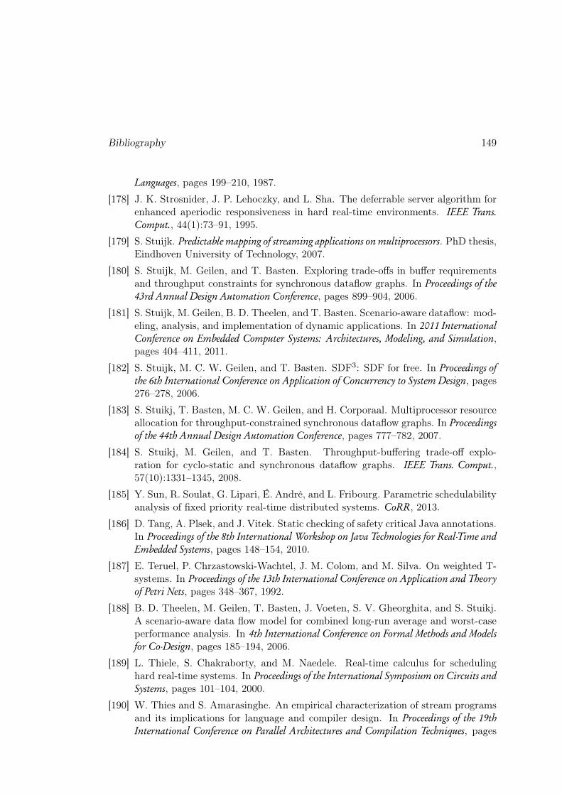
Bibliography 149
Languages, pages 199–210, 1987.
[178] J. K. Strosnider, J. P. Lehoczky, and L. Sha. The deferrable server algorithm forenhanced aperiodic responsiveness in hard real-time environments. IEEE Trans.Comput., 44(1):73–91, 1995.
[179] S. Stuijk. Predictable mapping of streaming applications on multiprocessors. PhD thesis,Eindhoven University of Technology, 2007.
[180] S. Stuijk, M. Geilen, and T. Basten. Exploring trade-offs in buffer requirementsand throughput constraints for synchronous dataflow graphs. In Proceedings of the43rd Annual Design Automation Conference, pages 899–904, 2006.
[181] S. Stuijk, M. Geilen, B. D. Theelen, and T. Basten. Scenario-aware dataflow: mod-eling, analysis, and implementation of dynamic applications. In 2011 InternationalConference on Embedded Computer Systems: Architectures, Modeling, and Simulation,pages 404–411, 2011.
[182] S. Stuijk, M. C. W. Geilen, and T. Basten. SDF3: SDF for free. In Proceedings ofthe 6th International Conference on Application of Concurrency to System Design, pages276–278, 2006.
[183] S. Stuikj, T. Basten, M. C. W. Geilen, and H. Corporaal. Multiprocessor resourceallocation for throughput-constrained synchronous dataflow graphs. In Proceedingsof the 44th Annual Design Automation Conference, pages 777–782, 2007.
[184] S. Stuikj, M. Geilen, and T. Basten. Throughput-buffering trade-off explo-ration for cyclo-static and synchronous dataflow graphs. IEEE Trans. Comput.,57(10):1331–1345, 2008.
[185] Y. Sun, R. Soulat, G. Lipari, É. André, and L. Fribourg. Parametric schedulabilityanalysis of fixed priority real-time distributed systems. CoRR, 2013.
[186] D. Tang, A. Plsek, and J. Vitek. Static checking of safety critical Java annotations.In Proceedings of the 8th International Workshop on Java Technologies for Real-Time andEmbedded Systems, pages 148–154, 2010.
[187] E. Teruel, P. Chrzastowski-Wachtel, J. M. Colom, and M. Silva. On weighted T-systems. In Proceedings of the 13th International Conference on Application and Theoryof Petri Nets, pages 348–367, 1992.
[188] B. D. Theelen, M. Geilen, T. Basten, J. Voeten, S. V. Gheorghita, and S. Stuikj.A scenario-aware data flow model for combined long-run average and worst-caseperformance analysis. In 4th International Conference on Formal Methods and Modelsfor Co-Design, pages 185–194, 2006.
[189] L. Thiele, S. Chakraborty, and M. Naedele. Real-time calculus for schedulinghard real-time systems. In Proceedings of the International Symposium on Circuits andSystems, pages 101–104, 2000.
[190] W. Thies and S. Amarasinghe. An empirical characterization of stream programsand its implications for language and compiler design. In Proceedings of the 19thInternational Conference on Parallel Architectures and Compilation Techniques, pages

150 Bibliography
365–376, 2010.
[191] S. R. V. Zivojnovic and H. Meyr. Optimizing DSP programs using multirateretiming transformation. In Proceedings of EUSIPCO Signal Processing, 1994.
[192] J. E. Vuillemin. On circuits and numbers. IEEE Trans. Comput., 43:868–879, 1994.
[193] A. Wellings and M. Kim. Asynchronous event handling and safety critical Java.In Proceedings of the 8th International Workshop on Java Technologies for Real-Time andEmbedded Systems, pages 53–62, 2010.
[194] M. Wiggers, M. Bekooij, P. Jansen, and G. Smit. Efficient computation of buffercapacities for multi-rate real-time systems with back-pressure. In Proceedings ofthe 4th International Conference on Hardware/Software Codesign and System Synthesis,pages 10–15, 2006.
[195] M. H. Wiggers, M. J. G. Bekooij, and G. J. M. Smit. Efficient computation ofbuffer capacities for cyclo-static dataflow graphs. In Proceedings of the 44th AnnualDesign Automation Conference, pages 658–663, 2007.
[196] F. Zhang and A. Burns. improvement to quick processor-demand analysis forEDF-scheduled real-time systems. In Proceedings of the 21st Euromicro Conferenceon Real-Time Systems, pages 76–86, 2009.
[197] F. Zhang and A. Burns. Schedulability analysis for real-time systems with EDFscheduling. IEEE Transactions on Computers, 58:1250–1258, 2009.
[198] X.-Y. Zhu, T. Basten, M. Geilen, and S. Stuikj. Efficient retiming of multirateDSP algorithms. IEEE Trans. on Computer-Aided Design of Integrated Circuits andSystems, 31(6):831–844, 2012.
[199] X.-Y. Zhu, M. Geilen, T. Basten, and S. Stuikj. Static rate-optimal scheduling ofmultirate DSP algorithms via retiming and unfolding. In Proceedings of 18th RealTime and Embedded Technology and Applications Symposium, pages 109–118, 2012.

Appendix A
Sets, orders, and sequences
This appendix introduces some basic mathematical concepts about ordered sets usedin describing the different dataflow models of computation. Most of definitions aretaken from the wonderful book of Davey and Priestly [65]. Furthermore, the appendixpresents the sequence domain and its properties.
A.1 Ordered sets
Definition A.1 (Poset). A partially ordered set (poset for short) is a pair (A,⊑) suchthat A is a set and ⊑ is a partial order relation on A (i.e. ⊑ is reflexive, antisymmetric,and transitive).
Definition A.2 (Maximal elements, the maximum). Let B be a subset of a poset(A,⊑). Then a ∈ B is a maximal element of B if a ⊑ b and b ∈ B imply a = b. The setof maximal elements of B is denoted by Max(B). The maximum element of B, if any,is max(B) ∈ B such that ∀a ∈ B : a ⊑max(B).
Dually, we can define the minimal elements and the minimum of a subset. Themaximum element of the poset, if any, is called the top element (denoted by ⊤A); whilethe minimum element, if any, is called the bottom element (denoted by ⊥A).
Definition A.3 (Upper bounds, the least upper bound). Let B be a subset of a poset(A,⊑). The set of upper bounds of B is Bu = {a ∈ A|∀b ∈ B : b ⊑ a}. The least upperbound of B, if any, is the minimum of Bu and it is denoted by
⊔
B.
Dually, we can define the set of lower bounds Bl and the greatest lower bounddB
of a subset B.
Definition A.4 (Join semi-lattice). A join semi-lattice (A,⊑,⊔) is a poset (A,⊑) suchthat any two elements a, b ∈ A have a least upper bound a ⊔ b (i.e.
⊔{a, b}).
Dually, we can define a meet semi-lattice. A lattice (A,⊑,⊔,⊓) is both a join semi-lattice and a meet semi-lattice.
151

152 Sets, orders, and sequences
Definition A.5 (complete lattice). A complete lattice (A,⊑,⊔,d) is a poset (A,⊑)such that any subset B ⊆ A has a least upper bound
⊔
B and a greatest lower bounddB in A.
Definition A.6 (Ascending chain condition). A chain B of a poset (A,⊑) is a subsetB ⊆ A such that ∀a, b ∈ B : (a ⊑ b) ∨ (b ⊑ a). The poset satisfies the ascendingchain condition (ACC) if and only if any infinite sequence a0 ⊑ a1 ⊑ . . . ⊑ an ⊑ . . . ofelements of A is not strictly increasing, that is ∃k ≥ 0 : ∀j ≥ k : ak = aj .
Definition A.7 (CPO). A complete partial order (CPO for short) (A,⊑,⊥A) is aposet (A,⊑) with a bottom ⊥A such that any increasing chain of A has a lower upperbound in A.
A.2 Fixed point theory
Definition A.8 (Monotone function). Let f ∈ A→ A be a (total) function on a poset(A,⊑,⊔,d). f is monotone if and only if ∀a, b ∈ A : a ⊑ b⇒ f(a) ⊑ f(b).
Definition A.9 (Fixed points). Consider f ∈ A→ A with (A,⊑) a poset, an elementa ∈ A is (1) a fixed point if and only if f(a) = a; (2) the greatest fixed point if and onlyif f(a) = a and ∀b : f(b) = b ⇒ b ⊑ a; (3) the least fixed point if and only f(a) = aand ∀b : f(b) = b⇒ a ⊑ b.
Theorem A.1 (Knaster-Tarski). A monotone function f ∈ A → A, with (A,⊑) acomplete lattice, has a least fixed point lfp(f) =
d{a ∈ A|f(a) ⊑ a}.
Definition A.10 (continuous function). Let (A,⊑,⊔) be a CPO. A function f ∈ A→A is continuous if and only if for every chain B ⊆ A, we have that
⊔
f(B) = f(⊔
B).
Lemma A.1 (CPO of continuous functions). For CPOs (A,⊑1) and (B,⊑2), let[A → B] be the set of all continuous total functions from A to B. ([A → B],⊑) is aCPO where ∀f, g ∈ [A→ B], we have that f ⊑ g ⇔ ∀a ∈ A : f(a) ⊑2 g(a).
Theorem A.2 (fixed point theorem for a continuous function on a CPO). Let f ∈A→ A be a continuous function on a CPO (A,⊑,⊥A). The least fixed point exists andequals
⊔
n≥0 fn(⊥A) such that fn+1 = fn ◦ f .
Theorem A.3 (fixed point theorem for a monotone function on a CPO). Every mono-tone function on a CPO has a least fixed point.
A.3 Sequences
Let A∞ be the set of finite or denumerably infinite sequences over a set A. A finitesequence s ∈ A∗ is a total function s : {1, . . . , n} → A for some natural number n suchthat s(i) is the ith element of the sequence. The number n is the length of the sequence,denoted by |s|. The empty sequence, which has a length equal to 0, is denoted by ǫ. The

Tuples 153
sequence s : N>0 → A is an infinite sequence of length equals ω where ∀i ∈ N : i < ω.The set of infinite sequences is denoted by Aω. Thus, A∞ = A∗ ∪Aω.
We often list the elements of a sequence s, writing a1 a2 . . . a|s| if s ∈ A∗, anda1 a2 . . . if s ∈ Aω. For two sequences s1 and s2, the sequence s1.s2 represents theirconcatenation.
Definition A.11 (Prefix order). A sequence s1 is a prefix of a sequence s2, and wewrite s1 ⊑ s2, if and only if it exists s3 such that s2 = s1.s3. We say then that s1provides an approximate information about s2. The relation ⊑ is a partial order onA∞.
(A∞,⊑) is a CPO. Indeed, the poset (A∞,⊑) has a bottom element ⊥ = ǫ. Fur-thermore, the lower upper bound of any finite non-empty chain is the greatest element,while the lower upper bound of any infinite chain s0 ⊑ s1 ⊑ . . . ⊑ sn ⊑ . . . is the infinitesequence s where s(i) equals sk(i) for any k such that |sk| ≥ i.
(A∞,⊑) is a meet semi-lattice since the greatest lower bound of any two sequencesis their longest common prefix. However, it is not a join semi-lattice (e.g. a1 a2 anda2 a1 do not have a lower upper bound).
A.3.1 Periodic sequences
An infinite constant sequence s = aω where a ∈ A is a sequence such that ∀i ∈ N>0 :s(i) = a. A periodic infinite sequence s = vω, where v is a finite non-empty sequence, isa sequence such that ∀i ∈ N>0 : s(i) = v(1 + (i− 1) mod |v|). An ultimately periodicsequence s = uvω, where u is a (possibly empty) finite sequence, is the concatenation ofa periodic sequence vω to a finite sequence u. Hence, ∀i ∈ N>0 : s(i) = u(i) if i ≤ |u|;and s(i) = v(1+(i−|u|−1) mod |v|) otherwise. So, every constant sequence is periodic(|v| = 1) and every periodic sequence is ultimately periodic (|u| = 0).
A.4 Tuples
An N -tuple S ∈ A∞1 × A∞
2 × · · · × A∞N is a collection of N sequences si ∈ A∞
i . Weoften list the sequences within a N -tuple, writing [s1, s2, . . . , sN ]. Thus, S(i) representsthe ith sequence of the tuple. For the sake of conciseness, the Cartesian product A∞
1 ×A∞
2 × · · · ×A∞N is denoted by AN .
We extend the prefix order to AN as the point-wise prefix order; i.e. if S1, S2 ∈ AN ,then S1 ⊑ S2 if and only if ∀i : S1(i) ⊑i S2(i). Since any direct product of CPOs is aCPO, then (AN ,⊑,⊥) is a CPO such that ⊥ = [ǫ1, . . . , ǫN ].
A.5 Real sequences
Arithmetic operations are extended to real sequences as follows. If s and r are two in-finite sequences or finite sequences with |s| = |r|, then ∀i : (s op r)(i) = s(i) op r(i).Furthermore, s ≤ r if and only if ∀i : s(i) ≤ r(i).

154 Sets, orders, and sequences
Definition A.12 (Cumulative functions). The cumulative function of a real sequences ∈ R∞ is the sequence ⊕s such that ∀i ∈ {1, . . . , |s|} : ⊕s(i) =
∑ij=1 s(j). By
convention, ⊕s(0) = 0.
The sum of all elements of a finite sequence v ∈ R∗, denoted by ‖v‖, is equal to⊕v(|v|).Definition A.13 (Inverse sequence). Let s ∈ N∞ be an integer sequence. The inversesequence s−1 ∈ N∞ is the sequence such that ∀j ≤ ‖s‖ : ⊕s(s−1(j) − 1) < j ≤⊕s(s−1(j)). For example, if s = 1 2 4, then s−1(5) = 3 because ⊕s(2) < 5 ≤ ⊕s(3).Definition A.14 (⊗ operator). Let s ∈ Rω and r ∈ Nω be two infinite sequences. The
sequence s⊗ r ∈ Rω is defined as follows. ∀i ∈ N>0 : (s⊗ r)(i) =r(i)∑
j=1s(j +⊕r(i− 1)).
The on operator of the synchronous language Lucy-n [134] is equivalent to the⊗ operator defined on binary sequences Bω; i.e. the set of infinite sequences overB = {0, 1}. The set of ultimately periodic binary sequences corresponds to the set of2-adic numbers [192]. Table A.1 illustrates the ⊗ operator.
Table A.1: Illustration of ⊗ operator.
i 1 2 3 4 5 6 . . .
s 2 3 1 8 6 2 . . .⊕s 2 5 6 14 20 22 . . .r 0 2 1 0 0 2 . . .⊕r 0 2 3 3 3 5 . . .s⊗ r 0 5 1 0 0 14 . . .⊕(s⊗ r) 0 5 6 6 6 20 . . .
Property A.1. ⊕(s⊗ r) = (⊕s) ◦ (⊕r).Proof: From Definition A.14, we note that ∀i : (s⊗ r)(i) = ⊕s(⊕r(i))−⊕s(⊕r(i− 1)).
Hence, ⊕(s⊗ r)(i) =i∑
j=1⊕s(⊕r(j))−
i∑
j=1⊕s(⊕r(j − 1)) = ⊕s(⊕r(i)).
Property A.2. The set of ultimately periodic integer sequences N is closed under the⊗ operation.
Proof: Let s = u1vω1 and r = u2v
ω2 be two ultimately periodic sequences. We have that
∀i > |u1| : ⊕s(i+ |v1|) = ⊕s(i) + ‖v1‖ and ∀i > |u2| : ⊕r(i+ |v2|) = ⊕r(i) + ‖v2‖. Letus put
β =|v1|
gcd(|v1|, ‖v2‖), α = β|v2| , and γ =
‖v2‖gcd(|v1|, ‖v2‖)
So, ∀i > |u2| : ⊕r(i+ α) = ⊕r(i) + β‖v2‖ = ⊕r(i) + |v1|γ. Thus, ∃i0 : ∀i ≥ i0, we havethat

Real sequences 155
(s⊗ r)(i+ α) = ⊕s(⊕r(i+ α))−⊕s(⊕r(i− 1 + α))
= ⊕s(⊕r(i) + γ|v1|)−⊕s(⊕r(i− 1) + γ|v1|)= ⊕s(⊕r(i)) + γ‖v1‖ − ⊕s(⊕r(i− 1))− γ‖v1‖= (s⊗ r)(i)
Therefore, u1vω1 ⊗ u2vω2 = uvω with |v| = α and ‖v‖ = γ‖v1‖.
Property A.3. (N ,⊗, 1ω) is a monoid.
Proof: 1) Closure. ∀s, r ∈ N : s⊗ r ∈ N (Property A.2).2) Identity element. ∀s ∈ N : s⊗ 1ω = 1ω ⊗ s = s.3) Associativity. ∀s, r, t ∈ N :
(s⊗ (r ⊗ t))(i) = ⊕s((⊕(r ⊗ t))(i))−⊕s((⊕(r ⊗ t))(i− 1))
= ⊕s(⊕r(⊕t(i)))−⊕s(⊕r(⊕t(i− 1))) ( Property A.1)
= (⊕(s⊗ r))(⊕t(i))− (⊕(s⊗ r))(⊕t(i− 1))
= ((s⊗ r)⊗ t)(i)

156 Sets, orders, and sequences
List of Figures
1 Real-time scheduling of dataflow graphs. . . . . . . . . . . . . . . . . . . 42 (a) un graphe flot de données et (b) une relation d’activation. . . . . . . 83 Un ordonnancent abstrait inconsistant. . . . . . . . . . . . . . . . . . . . 94 Une relation d’activation affine de paramètres (4, 2, 3). . . . . . . . . . . 9
1.1 Example of (a) a cyclic SDF graph, and (b) its equivalent HSDF graph. 261.2 Reachability graph of the SDF example. . . . . . . . . . . . . . . . . . . 271.3 Self-timed execution of the SDF example. . . . . . . . . . . . . . . . . . 291.4 Retiming of a SDF graph. . . . . . . . . . . . . . . . . . . . . . . . . . . 321.5 Pareto space of the SDF example. . . . . . . . . . . . . . . . . . . . . . . 35
2.1 Time abstraction of the self-timed example. . . . . . . . . . . . . . . . . 542.2 Illustration of Proposition 2.1. . . . . . . . . . . . . . . . . . . . . . . . 572.3 Illustration of Lemma 2.2. . . . . . . . . . . . . . . . . . . . . . . . . . 582.4 Illustration of Proposition 2.2. . . . . . . . . . . . . . . . . . . . . . . . 592.5 Illustration of Proposition 2.3. . . . . . . . . . . . . . . . . . . . . . . . 602.6 Graph of activation relations. . . . . . . . . . . . . . . . . . . . . . . . . 612.7 Consistency of symmetric difference of simple cycles. . . . . . . . . . . . 622.8 Illustration of Proposition 2.6. . . . . . . . . . . . . . . . . . . . . . . . . 632.9 A (3,−4, 5)−affine relation. . . . . . . . . . . . . . . . . . . . . . . . . . 682.10 A consistent affine schedule. . . . . . . . . . . . . . . . . . . . . . . . . 712.11 Function cbefi,k: partitioned fixed-priority scheduling. . . . . . . . . . . 732.12 Function cbefk,i: partitioned fixed-priority scheduling. . . . . . . . . . . 752.13 Function cbefi,k: partitioned EDF scheduling, νi = νk. . . . . . . . . . . 772.14 An ultimately cyclo-static dataflow graph. . . . . . . . . . . . . . . . . 792.15 (a) An UCSDF graph and (b) its equivalent CSDF graph. . . . . . . . . 792.16 Linear bounds of ultimately periodic rates. . . . . . . . . . . . . . . . . 802.17 Activation relations of the schedule p2 p3 p3 p1 p2(p2 p3 p3 p1 p3 p1)ω. . 812.18 (a) An UCSDF graph with a multichannel and (b) its equivalent graph
with simple channels. . . . . . . . . . . . . . . . . . . . . . . . . . . . . 822.19 Buffer minimization using a shared storage space. . . . . . . . . . . . . . 832.20 A synchronous execution of process p. . . . . . . . . . . . . . . . . . . . 85
3.1 Priority assignment problem expressed as a LOP. . . . . . . . . . . . . . 923.2 Partitioning of the T -space into a set of DM priority regions. . . . . . . 93
157

158 List of Figures
3.3 Transforming DM priority assignments. . . . . . . . . . . . . . . . . . . 943.4 Exploration of the priority orderings space: throughput vs buffering re-
quirements. . . . . . . . . . . . . . . . . . . . . . . . . . . . . . . . . . . 953.5 Exploration of the priority orderings space: throughput vs precedence
distance. . . . . . . . . . . . . . . . . . . . . . . . . . . . . . . . . . . . . 963.6 Exploration of the priority orderings space: throughput vs utilization
distance. . . . . . . . . . . . . . . . . . . . . . . . . . . . . . . . . . . . . 963.7 Illustration of DF-B&B symbolic FP schedulability analysis. . . . . . . . 1003.8 Totally ordered communication strategy. . . . . . . . . . . . . . . . . . . 1033.9 safri,k function. . . . . . . . . . . . . . . . . . . . . . . . . . . . . . . . . 1033.10 Deadlines computation example. . . . . . . . . . . . . . . . . . . . . . . 1043.11 Illustration of SQPA. . . . . . . . . . . . . . . . . . . . . . . . . . . . . . 1073.12 Illustration of DF-B&B SQPA. . . . . . . . . . . . . . . . . . . . . . . . 1093.13 Illustration of ffdbf . . . . . . . . . . . . . . . . . . . . . . . . . . . . . . 111
4.1 Achieved throughput in EDF/RM uniprocessor scheduling. . . . . . . . . 1154.2 Impact of number of processors on the throughput in BF-RM scheduling. 1174.3 Comparison between BF-EDF and the first fit allocation strategy of DARTS.1174.4 Comparison between BF-EDF and FFDBF-SQPA. . . . . . . . . . . . . . 1184.5 Comparison between DARTS and ADFG in terms of buffering requirements.1194.6 Impact of the totally ordered communication strategy on the buffering
requirements. . . . . . . . . . . . . . . . . . . . . . . . . . . . . . . . . . 1194.7 Impact of the LOP priority assignment on the buffering requirements and
the processor utilization. . . . . . . . . . . . . . . . . . . . . . . . . . . . 1204.8 Impact of the constrained LOP priority assignment on the buffering re-
quirements and the processor utilization. . . . . . . . . . . . . . . . . . . 1204.9 Impact of the priority assignment with utilization distance on the buffer-
ing requirements and the processor utilization. . . . . . . . . . . . . . . . 1214.10 Performance of the SQPA algorithm. . . . . . . . . . . . . . . . . . . . . 1224.11 Impact of constrained deadlines on the performance of the SQPA algorithm.1234.12 Performance of the FFDBF-SQPA algorithm. . . . . . . . . . . . . . . . . 1244.13 Impact of the number of processors on the performance of the FFDBF-SQPA
algorithm. . . . . . . . . . . . . . . . . . . . . . . . . . . . . . . . . . . . 1244.14 Performance of the DF-B&B SQPA algorithm. . . . . . . . . . . . . . . . 1254.15 Performance of the SRTA algorithm. . . . . . . . . . . . . . . . . . . . . 1264.16 Performance of the DF-B&B SRTA algorithm. . . . . . . . . . . . . . . . 1264.17 SCJ mission life cycle. . . . . . . . . . . . . . . . . . . . . . . . . . . . . 1284.18 An ultimately cyclo-static dataflow graph with aperiodic actors. . . . . . 1294.19 Graphical editor for SCJ/L1 applications design. . . . . . . . . . . . . . 130


Abstract
The ever-increasing functional and nonfunctional requirements in real-time safety-criticalembedded systems call for new design flows that solve the specification, validation, and syn-thesis problems. Ensuring key properties, such as functional determinism and temporal pre-dictability, has been the main objective of many embedded system design models. Dataflowmodels of computation (such as KPN, SDF, CSDF, etc.) are widely used to model stream-based embedded systems due to their inherent functional determinism. Since the introduc-tion of the (C)SDF model, a considerable effort has been made to solve the static-periodicscheduling problem. Ensuring boundedness and liveness is the essence of the proposed al-gorithms in addition to optimizing some nonfunctional performance metrics (e.g. bufferminimization, throughput maximization, etc.). However, nowadays real-time embeddedsystems are so complex that real-time operating systems are used to manage hardware re-sources and host real-time tasks. Most of real-time operating systems rely on priority-drivenscheduling algorithms (e.g. RM, EDF, etc.) instead of static schedules which are inflexibleand difficult to maintain. This thesis addresses the real-time scheduling problem of dataflowgraph specifications; i.e. transformation of the dataflow specification to a set of independentreal-time tasks w.r.t. a given priority-driven scheduling policy such that the following prop-erties are satisfied: (1) channels are bounded and overflow/underflow-free; (2) the task set isschedulable on a given uniprocessor (or multiprocessor) architecture. This problem requiresthe synthesis of scheduling parameters (e.g. periods, priorities, processor allocation, etc.)and channel capacities. Furthermore, the thesis considers two performance optimizationproblems: buffer minimization and throughput maximization.
Résumé
Les systèmes temps-réel critiques sont de plus en plus complexes, et les exigences fonction-nelles et non-fonctionnelles ne cessent plus de croître. Le flot de conception de tels sys-tèmes doit assurer, parmi d’autres propriétés, le déterminisme fonctionnel et la prévisibilitétemporelle. Le déterminisme fonctionnel est inhérent aux modèles de calcul flot de don-nées (ex. KPN, SDF, etc.) ; c’est pour cela qu’ils sont largement utilisés pour modéliserles systèmes embarqués de traitement de flux. Un effort considérable a été accompli pourrésoudre le problème d’ordonnancement statique périodique et à mémoire de communica-tion bornée des graphes flots de données. Cependant, les systèmes embarqués temps-réeloptent de plus en plus pour l’utilisation de systèmes d’exploitation temps-réel et de stratégiesd’ordonnancement dynamique pour gérer les tâches et les ressources critiques. Cette thèseaborde le problème d’ordonnancement temps-réel dynamique des graphes flot de données ; ceproblème consiste à assigner chaque acteur dans un graphe à une tâche temps-réel périodique(i.e. calcul des périodes, des phases, etc.) de façon à : (1) assurer l’ordonnançabilité des tâchessur une architecture et pour une stratégie d’ordonnancement (ex. RM, EDF) données ; (2)exclure statiquement les exceptions d’overflow et d’underflow sur les buffers de communica-tion ; et (3) optimiser les performances du système (ex. maximisation du débit, minimisationdes tailles des buffers).


![Efficient Scheduling of Arbitrary Task Graphs to Multiprocessors …ranger.uta.edu/~iahmad/journal-papers/[J16]Efficient... · 2002-10-23 · - 1 - Efficient Scheduling of Arbitrary](https://static.fdocuments.net/doc/165x107/5edac4a4fa3b3a5ad2169208/eficient-scheduling-of-arbitrary-task-graphs-to-multiprocessors-iahmadjournal-papersj16efficient.jpg)


![Real-time scheduling of dataflow graphs · Adnan Bouakaz. Real-time scheduling of dataflow graphs. Other [cs.OH]. Université Rennes 1, 2013. English. NNT: 2013REN1S103 . tel-00945453](https://static.fdocuments.net/doc/165x107/603c6d77a65f9240f444d911/real-time-scheduling-of-dataflow-graphs-adnan-bouakaz-real-time-scheduling-of-dataflow.jpg)
