Real time Monitoring and Forecasting of Ecological Processes
7
Real–time Monitoring and Forecasting of Ecological Processes J. Culiţă, A. Dumitraşcu, D. Ştefănoiu Automatic Control and Computers Faculty, “Politehnica” University of Bucharest, Romania (e-mails: [email protected] , [email protected] , [email protected] ) Abstract: The paper introduces a real-time monitoring and forecasting system for ecological phenomena. The process yields a collection of ecological parameters viewed as distributed time series, which are measured by means of wireless network of sensors. The acquired data are preliminary processed and modeled by using complex algorithms in view of prediction. There are three graphical user interfaces implemented within the monitoring and forecasting system: eko-View and eko-Greenhouse (which directly interacts with the process) and eko-Forecast (which estimates the future evolution of some ecological parameters). The monitoring system was effectively integrated in an industrial application dealing with automatic irrigation of a small greenhouse. The forecasting simulation results with real data and a comparative assessment of predictor performances are presented in the end. Keywords: real-time remote monitoring, forecasting, distributed control architecture, greenhouse control 1. INTRODUCTION Rapid climate changes and the negative impact of industry upon the environment require designing and employing of an automatic monitoring system of geographical areas. The general purpose of monitoring is to forecast the behavior of the ecological system in view of disaster anticipation or avoidance. The ecological phenomena could be evidenced either in an open space or in an enclosed space. Phenomena like correlation between temperature variation and humidity or heat and humidity transfer usually occur in a greenhouse. Especially in a microclimate, ambient temperature and humidity, dew point and solar radiation are quite correlated, which could improve their prediction accuracy. The soil parameters (moisture, temperature, water content, leaf wetness) are however less correlated. The paper mainly presents an ecological monitoring and forecasting system EcoMonFor, which allows mon itoring and for ecasting of multi-variable eco logical signals both in local and wider geographical regions. EcoMonFor was successfully integrated in a new application on remote monitoring and control of a small greenhouse (Dumitrascu, 2010). Basically, the application aim is the automatic watering of plants, when the ecological state requires it, in order to yield suitable growth of plants. The distributed monitoring and control architecture of the ecological process interconnects several subsystems (see figure 1). The first one is a wireless acquisition and monitoring subsystem structured on three hierarchical levels (Culita and Stefanoiu, 2010) and provided with three graphical user-friendly interfaces eKo- View, eko-Greenhouse and eko-Forecast. The second one is the automatic control subsystem made of PLCs and industrial communication networks. Finally, the irrigation subsystem consists of two water tanks, sensors and actuators. This article is not pointing to control design. Data monitoring and preparing in view of prediction, together with forecasting results are discussed here only. In our approach, the ecological signal prediction relies on numerical models that were previously implemented as FORWAVER, PARMA, PARMAX, KARMA predictors (Stefanoiu et al, 2008; Stefanoiu and Culita, 2010). It is expected that the forecasting experimental results to be quite accurate especially when the ecological parameter supplied by the greenhouse are correlated to each other. The paper is structured as follows. Section 2 introduces the distributed architecture for monitoring and control of the greenhouse. Section 3 presents the acquisition and preliminary processing of the ecological parameters provided by the greenhouse. The performances of prediction are shown within Section 4. A conclusion and the references list complete the article. 2. MONITORING AND CONTROL SYSTEM ARCHITECTURE OF THE GREENHOUSE The greenhouse consists of six plants which are located in two separated laboratory rooms in order to create different microclimates. The improper care of plants led to constructing an automatic irrigation system. Figure 1 depicts the distributed monitoring and control architecture of the greenhouse, which integrates: the automatic control system of irrigation (left side down), the irrigation system (left side up) and, most concerned, the ecological monitoring system EcoMonFor (right side). Constructively, EcoMonFor was separated in two components: a mobile part, referred to as EcoMonFor-M, figured inside the (red) ellipsis and a fixed part, namely EcoMonFor-F, represented in the right down corner. The mobile monitoring system is structured on three hierarchical levels as shown in the right upper side of figure 1:
Transcript of Real time Monitoring and Forecasting of Ecological Processes

Real–time Monitoring and Forecasting of Ecological Processes
J. Culiţă, A. Dumitraşcu, D. Ştefănoiu
Automatic Control and Computers Faculty, “Politehnica” University of Bucharest, Romania
(e-mails: [email protected], [email protected], [email protected])
Abstract: The paper introduces a real-time monitoring and forecasting system for ecological phenomena.
The process yields a collection of ecological parameters viewed as distributed time series, which are
measured by means of wireless network of sensors. The acquired data are preliminary processed and
modeled by using complex algorithms in view of prediction. There are three graphical user interfaces
implemented within the monitoring and forecasting system: eko-View and eko-Greenhouse (which
directly interacts with the process) and eko-Forecast (which estimates the future evolution of some
ecological parameters). The monitoring system was effectively integrated in an industrial application
dealing with automatic irrigation of a small greenhouse. The forecasting simulation results with real data
and a comparative assessment of predictor performances are presented in the end.
Keywords: real-time remote monitoring, forecasting, distributed control architecture, greenhouse control
1. INTRODUCTION
Rapid climate changes and the negative impact of industry
upon the environment require designing and employing of an
automatic monitoring system of geographical areas. The
general purpose of monitoring is to forecast the behavior of
the ecological system in view of disaster anticipation or
avoidance.
The ecological phenomena could be evidenced either in an
open space or in an enclosed space. Phenomena like
correlation between temperature variation and humidity or
heat and humidity transfer usually occur in a greenhouse.
Especially in a microclimate, ambient temperature and
humidity, dew point and solar radiation are quite correlated,
which could improve their prediction accuracy. The soil
parameters (moisture, temperature, water content, leaf
wetness) are however less correlated.
The paper mainly presents an ecological monitoring and
forecasting system EcoMonFor, which allows monitoring
and forecasting of multi-variable ecological signals both in
local and wider geographical regions. EcoMonFor was
successfully integrated in a new application on remote
monitoring and control of a small greenhouse (Dumitrascu,
2010). Basically, the application aim is the automatic
watering of plants, when the ecological state requires it, in
order to yield suitable growth of plants. The distributed
monitoring and control architecture of the ecological process
interconnects several subsystems (see figure 1). The first one
is a wireless acquisition and monitoring subsystem structured
on three hierarchical levels (Culita and Stefanoiu, 2010) and
provided with three graphical user-friendly interfaces eKo-
View, eko-Greenhouse and eko-Forecast. The second one is
the automatic control subsystem made of PLCs and industrial
communication networks. Finally, the irrigation subsystem
consists of two water tanks, sensors and actuators.
This article is not pointing to control design. Data monitoring
and preparing in view of prediction, together with forecasting
results are discussed here only. In our approach, the
ecological signal prediction relies on numerical models that
were previously implemented as FORWAVER, PARMA,
PARMAX, KARMA predictors (Stefanoiu et al, 2008;
Stefanoiu and Culita, 2010). It is expected that the forecasting
experimental results to be quite accurate especially when the
ecological parameter supplied by the greenhouse are
correlated to each other.
The paper is structured as follows. Section 2 introduces the
distributed architecture for monitoring and control of the
greenhouse. Section 3 presents the acquisition and
preliminary processing of the ecological parameters provided
by the greenhouse. The performances of prediction are shown
within Section 4. A conclusion and the references list
complete the article.
2. MONITORING AND CONTROL SYSTEM
ARCHITECTURE OF THE GREENHOUSE
The greenhouse consists of six plants which are located in
two separated laboratory rooms in order to create different
microclimates. The improper care of plants led to
constructing an automatic irrigation system. Figure 1 depicts
the distributed monitoring and control architecture of the
greenhouse, which integrates: the automatic control system of
irrigation (left side down), the irrigation system (left side up)
and, most concerned, the ecological monitoring system
EcoMonFor (right side).
Constructively, EcoMonFor was separated in two
components: a mobile part, referred to as EcoMonFor-M,
figured inside the (red) ellipsis and a fixed part, namely
EcoMonFor-F, represented in the right down corner. The
mobile monitoring system is structured on three hierarchical
levels as shown in the right upper side of figure 1:

Fig. 1. Architecture of the small greenhouse control system including EcoMonFor
the set of wireless eko-sensors; eko-Gateway – a centralizing
(kernel) equipment of the sensor network; a computer (or
laptop). The last two components are wirelessly connected to
Internet, in order to enable running remote applications.
Moreover, the computer fulfils the function of real-time video
supervision of the whole system through a coupled webcam.
EcoMonFor-M mostly is responsible for remote data
acquisition and monitoring, which means it could cover an
extended geographical area. It can be employed for a quick
prediction of the measured data, as well. The data collection
supplied by eko-Gateway module is sent to EcoMonFor-F
with the aim of high quality prediction of the ecological
phenomena. This strategy is suggested by the curved arrow in
the bottom of the image. The core of the fixed component
consists in a parallel computer with 16 processors. This is
connected via internet to an extensible computer network.
The central unit is hosting complex algorithms for modeling,
identification and forecasting of distributed ecological
signals: PARMA, PARMAX, KARMA and FORWAVER.
Both components of EcoMonFor are working on the
following strategy: first, the acquisition and the preliminary
processing of data are performed. Sometimes, data provided
by sensors are damaged and need to be enhanced. Some
operations are necessary to improve data (as shown within
the next section). The visual monitoring of the greenhouse
stands for the second step, which is executed in parallel with
the acquisition and is remotely performed by eko-Gateway.
Two web graphical user interfaces are implemented on the
computer connected to eko-Gateway. The first one, eko-
View, gives the user the ability to set and display the
configuration of the sensor network and then to start
monitoring and acquisition, from anywhere in the world.
Moreover, it is supplied with several facilities in handling
data (i.e. graphical display of interest data, exporting to
common programming environments, setting alerting rules).
The sensor configuration on the real case study will be
exemplified in the next section. The second web interface is
eKo-Greenhouse, as displayed by figure 2. This is more
oriented towards the irrigation application. Thus, its role is
helping the user to directly and remotely interact with the
greenhouse, via internet, by accessing the process parameters
and controlling the automatic irrigation system. Technically,
the main panel is based on Apache http server and it is
password protected. It was built using common Web
technologies: HTML, JavaScript, XML PHP. The interface
configuration displays four interesting zones: on the left side
above, the visual image of the process is permanently offered
by a webcam; beneath, the results of the last 10 commands to
the actuators are completely shown; at right, four selection
buttons are depicted for choosing a corresponding control
panel (i.e, commands to the control device PLC S7-300;
remote commands for manual control of actuators in the
irrigation process and information about the current status of
them; displaying and setting the ecological parameters by the
user; exporting data from eko-Gateway in a comprehensible
and useful format and saving them on external disk, for
subsequent processing).
The final step of the operating strategy of EcoMonFor system
corresponds to data modeling on prediction purpose. A
convivial graphical interface eKo-Forecast was implemented
in MATLAB programming language, in order to complete a
forecasting experiment (Culita and Stefanoiu, 2010).
Ball and filter
valve for manual
closing
NO electro-
valve
Water
supply
Float-type
locking element
Water
filter
Irrigation tank
maximum level
detection sensor
medium level
detection sensor
minimum level
detection sensor
PROFINET Bus
MPI Bus
Manual commands for
actuators
PLC inputs
Outp
uts
com
man
ds
to a
ctuat
ors
ASI Bus
Outp
uts
for
war
nin
g L
ED
Room 1
Wwireless
eko-nodes
NC electro-
valve
Soil moisture
sensors
Room 2
eko-radio base
eko-Gateway
USB cable
External HDD
maximum level
detection sensor
medium level
detection sensor
minimum level
detection sensor
Buffer tank
Web video
camera
4 quad processors
SUPERMICRO Superserver
Parallel Machine
1 dual core processor
ASSUS PC
Pump
OP 177B Scalance
X208
PLC S7-300

Fig. 2. The web interface eko-Greenhouse, yielding the remote control
It facilitates running PARMA, PARMAX, KARMA and
FORWAVER predictors within FORTIS (FORecasting of
TIme Series) simulator. The interface offers a graphical
illustration of the forecasting results. Although all predictors
can proceed on the same fixed or mobile component either,
the faster predictors of FORTIS (PARMA and FORWAVER)
are commonly hosted by the mobile entity and the slower
algorithms, PARMAX and KARMA, are usually executed on
the fixed component.
EcoMonFor system represents an additional part of the
irrigation application. One hand, it decides the irrigation
commands by acting through the sensor subsystem. On the
other hand it processes the measured data to forecast them.
3. DATA ACQUISITION AND PRELIMINARY
PROCESSING
As mentioned before, the greenhouse consists of 6 plants,
which are located in two different rooms. Each plant was
associated to a wireless node for acquisition and monitoring
purpose. The monitoring can be carried out by using eko-
View and eko-Greenhouse interfaces. Figure 3 illustrates the
main panel of eko-View interface. The plants are represented
by their photos. Every node is capable of transmitting data
from at most 4 sensors, while a sensor can measure 1-3
ecological parameters simultaneously (for example, there is a
singleton sensor for soil moisture and humidity or for
ambient humidity, temperature and dew point). Though, the
number of the ecological parameters differs for each sensor.
Figure 3 also shows the synoptic map of the monitored
ecological parameters associated to each acquisition node.
There have been used 21 sensors, which are transmitting data
for 33 ecological parameters, as it can be noticed from the
figure. As a major aim of monitoring, we are interested in
forecasting some ecological parameters of the greenhouse
and validating (testing) the correlations between them. In
order to send data to FORTIS simulator (in view of
prediction), the parameter values (of the same node) have to
be grouped in data blocks, according to their possible
correlations. For example, humidity is correlated to
temperature which, in its turn, is correlated to solar radiation.
It is rather difficult to presume that the soil parameters
coming from different plants are correlated each other, taking
into account that the plants lie in different locations. Each
block corresponds to a node and contains data from 3-4
acquisition channels. The name of such data block is an
identification code including: node identity (1-6); parameter
type (soil or ambient); the acronyms of the measured
parameters. For further processing (modeling and
forecasting), the data blocks need to be converted in
structures accepted by MATLAB programming environment.
Figure 3, as well as table 1, indicates all the observed
parameters of the small greenhouse. One can also see their
varying range and measurement units in table 1. Parameters
acronyms were set for data indexing and identification
purposes.
Table 1. Ecological parameters of sensors network.
Soil Leaves Ambient
Moisture (Mo)
0 ... 240 [cbar]
Leaf Wetness
(LeWe)
0 ... 1024 [CntS]
Humidity (Hu)
0 ... 100 [%]
Temperature (Te)
–40 ... +65 [°C]
Temperature (Te)
–40 ... +65 [°C]
Water Content
(WaCo)
0 ... 100 [%wfv]
Dew Point
(DwPo)
–10 ... 50 [°C]
Solar Radiation
(SoRa)
0 ... 1800 [W/m2]
The ecological sensors usually provide unsynchronized or
faulty data. Therefore, preliminary data processing is
necessary. A simple and intuitive method of obtaining
synchronized data is the hourly averaging technique.
Frequently, there could be missing data on different
acquisition channels at some instants. In this case, the
interpolation followed by re-sampling can return correct data.
First, for isolated missing information, linear interpolation is
enough, as it can be noticed from inspecting figure 4 (raw
data) and figure 5 (linear interpolated data). Next, for the
other lost data (that extends over an interval of sampling
instants), autoregressive interpolation (AR) seems to be quite
adequate (see results in figure 6). The AR model was
identified by applying Levinson-Durbin Algorithms
(Soderstrom and Stoica, 1989).
PLC command
Variables monitoring
Manual command
Export data
eko-Greenhouse
Time [s]
Variables
Command
Room 1
Room 2
Room 1
Room 2
Room 1
Room 2

Fig. 3. Synoptic map of the monitored ecological parameters inside the greenhouse
Fig. 4. Raw data for leaf wetness parameter
Fig. 5. Linear interpolated data for leaf wetness
Fig. 6. AR interpolation of data for leaf wetness
There also occurs over-sampling phenomena, which means
gathering much many samples than necessary. Here, an
under-sampling technique is applied (for example,
averaging). In our case, the data were averaged over
3-4 hours, especially for prediction, since the evolution of
ecological phenomena is rather slow. Unlike before, it hardly
happens that data contain important discrepancies
(deviations) on short time intervals. These errors are
eliminated by numerical filtering. One of the matching filters
is second type Cebyshev (Proakis and Manolakis, 1996). For
the ecological parameters this filter was indirectly applied
with the aim of a refined delimitation between the
deterministic and nondeterministic components of the
prediction model.
Soil Leaves
WaCo LeWe
Mo Te
Soil Ambient WaCo Hu
Mo Te
Te DwPo
SoRa
Soil Leaves WaCo LeWe
Mo Te
Soil Leaves Ambient
Mo LeWe Hu
Te Te
DwPo
Soil Leaves
WaCo LeWe
Mo Te
Soil Ambient
WaCo Hu
Mo Te
Te DwPo
SoRa
4. SIMULATION RESULTS
The automatic irrigation application intended to improve the
comfort and health of plants in the greenhouse, relatively to
the situation of inappropriate watering. For the automatic
control application, the parameters of interest are: soil
moisture (Mo) and soil water content (WaCo). However, both
parameters are correlated with soil temperature (Te).
Therefore soil Te is one of the parameters to be
predicted/monitored. Our simulations are focusing next on
this parameter only (although in correlation with the other
soil parameters).
The forecasting of greenhouse parameters is performed by
means of PARMA, PARMAX, KARMA and FORWAVER
predictors. A collection of 30 data blocks has been employed
to predict various parameters. The data blocks resulted from
combinations of soil or ambient parameters, as shown by the
synoptic map of figure 3. The PARMAX predictor was the
most employed since it has to be run several times for each
channel. In order to reduce the simulation time, the
EcoMonFor-F computer network was extended up to 16 PCs,
including the laptop of EcoMonFor-M. The ecological
phenomena usually act slowly. Therefore it is suitable to
predict values every 3-4 hours. The simulation time for
predictors varied between several minutes and several tens of
hours, depending on their complexity, the number of
analyzed ecological data and the modeling of stochastic
component. Each one of the 30 data files is associated to 16
graphics for every acquisition channel, coming from all four
predictors. There are 4 variations for a channel, which are
bond to a predictor performance: the original data (time
series) together with its optimal trend, the estimated white
noise on measuring horizon; the predicted values and the
prediction quality (Stefanoiu and Culita, 2010). Each
predicted value has a trusting probability defined by the
confidence tube. As the prediction instant goes away from the
measuring horizon, the tube becomes larger and larger. This
means the predicted values are less and less reliable.
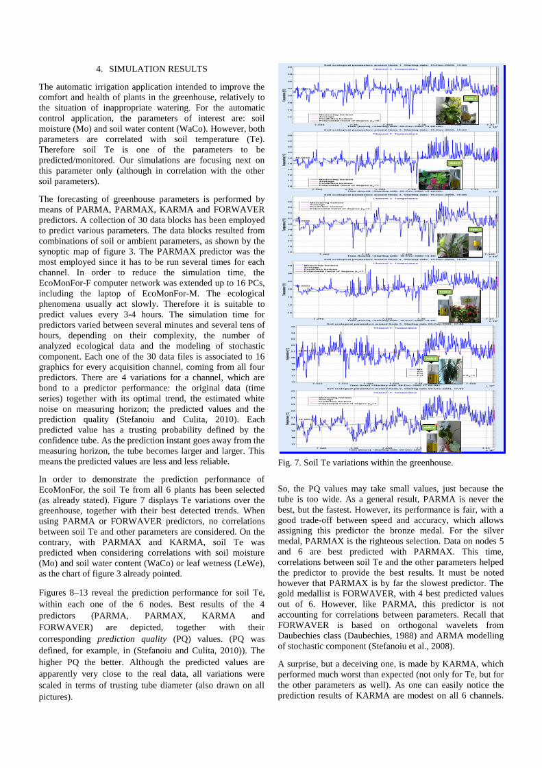
In order to demonstrate the prediction performance of
EcoMonFor, the soil Te from all 6 plants has been selected
(as already stated). Figure 7 displays Te variations over the
greenhouse, together with their best detected trends. When
using PARMA or FORWAVER predictors, no correlations
between soil Te and other parameters are considered. On the
contrary, with PARMAX and KARMA, soil Te was
predicted when considering correlations with soil moisture
(Mo) and soil water content (WaCo) or leaf wetness (LeWe),
as the chart of figure 3 already pointed.
Figures 8–13 reveal the prediction performance for soil Te,
within each one of the 6 nodes. Best results of the 4
predictors (PARMA, PARMAX, KARMA and
FORWAVER) are depicted, together with their
corresponding prediction quality (PQ) values. (PQ was
defined, for example, in (Stefanoiu and Culita, 2010)). The
higher PQ the better. Although the predicted values are
apparently very close to the real data, all variations were
scaled in terms of trusting tube diameter (also drawn on all
pictures).
Fig. 7. Soil Te variations within the greenhouse.
So, the PQ values may take small values, just because the
tube is too wide. As a general result, PARMA is never the
best, but the fastest. However, its performance is fair, with a
good trade-off between speed and accuracy, which allows
assigning this predictor the bronze medal. For the silver
medal, PARMAX is the righteous selection. Data on nodes 5
and 6 are best predicted with PARMAX. This time,
correlations between soil Te and the other parameters helped
the predictor to provide the best results. It must be noted
however that PARMAX is by far the slowest predictor. The
gold medallist is FORWAVER, with 4 best predicted values
out of 6. However, like PARMA, this predictor is not
accounting for correlations between parameters. Recall that
FORWAVER is based on orthogonal wavelets from
Daubechies class (Daubechies, 1988) and ARMA modelling
of stochastic component (Stefanoiu et al., 2008).
A surprise, but a deceiving one, is made by KARMA, which
performed much worst than expected (not only for Te, but for
the other parameters as well). As one can easily notice the
prediction results of KARMA are modest on all 6 channels.

A possible explanation resides in Kalman filter over-
sensitivity to the variation of internal states number. Just
removing or adding one single state can dramatically modify
the predicted values outside as well as inside the measure
horizon. The bronze-silver-gold classification is confirmed by
all tests, with different greenhouse parameters (although,
sometimes PARMAX is better than FORWAVER).
5. CONCLUSION
This article approached the problem of monitoring and
forecasting of small greenhouse parameters. In subsidiary, the
control system of greenhouse is also mentioned. The
monitoring system (namely, EcoMonFor) integrates three
user friendly interfaces eko-View, eko-Greenhouse and eko-
Forecast, which are implemented on a mobile or fixed web
computer. In order to model and predict the greenhouse
evolution, the measured parameters are collected in data
blocks depending on their correlation degree. Then, some
preliminary operations (interpolation, numerical filtering) are
applied for improving the quality of data. A comparative
study between four predictors performance (PARMA,
PARMAX, KARMA, FORWAVER) revealed that the best
accuracy of prediction is achieved by PARMAX; next come
PARMAX or PARMA, depending on the correlation degree
between the monitored ecological parameters.
REFERENCES
Dumitrascu, A. (2010). Contributions to industrial computer
networks in process control, PhD thesis, 218 pages,
“Politehnica” University of Bucharest.
Culita, J., Stefanoiu, D. (2010). FORTIS – An integrated
Simulator for Distributed Time Series Forecasting,
Industrial Simulation Conference ISC 2010, June 7-9,
2010, Budapest, Hungary, pp. 27-33.
Proakis, J.G., Manolakis, D.G. (1996). Digital Signal
Processing. Principles, Algorithms and Applications.,
third edition, Prentice Hall, Upper Saddle River, New
Jersey, USA.
Söderström, T., Stoica, P. (1989). System Identification,
Prentice Hall, London, U.K.
Stefanoiu, D., Culita, J. (2010). Multivariable Prediction of
Physical Data, PUB Scientific Bulletin, A Series, Vol. 72,
No. 1, pp. 95-102.
Stefanoiu, D., Culita, J., Ionescu, F. (2008). FORWAVER –
A Wavelet Based Predictor for Non Stationary Signals,
Industrial Simulation Conference ISC 2008, Lyon,
France, pp. 377-381.
Daubechies, I. (1988). Orthonormal Bases of Compactly
Supported Wavelets, Communications on Pure and
Applied Mathematics, No. XLI, pp. 909-996.
Fig. 8. Forecasting performance in node 1 (soil Te).
Fig. 9. Forecasting performance in node 2 (soil Te).
N1_Soil_WaCo.Mo.Te/PARMA: 65.65%
N1_Soil_WaCo.Mo.Te/PARMAX: 77.41%
N1_Soil_WaCo.Mo.Te/KARMA: 47.30%
N1_Soil_WaCo.Mo.Te/FORWAVER: 81.23%
N2_Soil_Mo.Te.LeWe/PARMA: 78.18%
N2_Soil_Mo.Te.LeWe/PARMAX: 77.49%
N2_Soil_Mo.Te.LeWe/KARMA: 57.46%
N2_Soil_Mo.Te.LeWe/FORWAVER: 79.34%
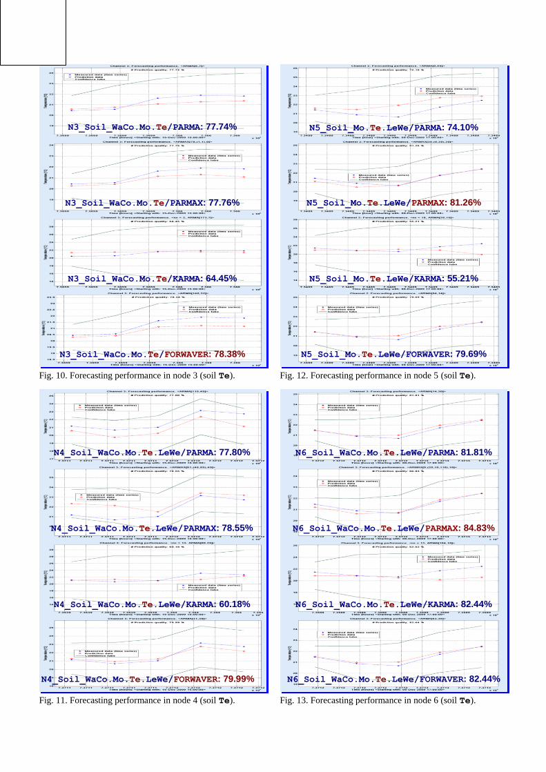
Fig. 10. Forecasting performance in node 3 (soil Te).
Fig. 11. Forecasting performance in node 4 (soil Te).
Fig. 12. Forecasting performance in node 5 (soil Te).
Fig. 13. Forecasting performance in node 6 (soil Te).
N3_Soil_WaCo.Mo.Te/PARMA: 77.74%
N3_Soil_WaCo.Mo.Te/PARMAX: 77.76%
N3_Soil_WaCo.Mo.Te/KARMA: 64.45%
N3_Soil_WaCo.Mo.Te/FORWAVER: 78.38%
N4_Soil_WaCo.Mo.Te.LeWe/PARMA: 77.80%
N4_Soil_WaCo.Mo.Te.LeWe/PARMAX: 78.55%
N4_Soil_WaCo.Mo.Te.LeWe/KARMA: 60.18%
N4_Soil_WaCo.Mo.Te.LeWe/FORWAVER: 79.99%
N5_Soil_Mo.Te.LeWe/FORWAVER: 79.69%
N5_Soil_Mo.Te.LeWe/PARMA: 74.10%
N5_Soil_Mo.Te.LeWe/PARMAX: 81.26%
N5_Soil_Mo.Te.LeWe/KARMA: 55.21%
N6_Soil_WaCo.Mo.Te.LeWe/PARMAX: 84.83%
N6_Soil_WaCo.Mo.Te.LeWe/PARMA: 81.81%
N6_Soil_WaCo.Mo.Te.LeWe/KARMA: 82.44%
N6_Soil_WaCo.Mo.Te.LeWe/FORWAVER: 82.44%