Real-time Kinematic Positioning: Background, Assessment ...

Real-time Kinematic Positioning:Background, Assessment and Forecasting

A thesis submitted to the faculty of the University of Minnesota by

John Jackson

In partial fulfillment of the requirements for the degree of Master of Science

Demoz Gebre-Egziabher

2018 July

Contents

List of Figures ii

List of Tables ii

1 Introduction 1

2 Background 4

2.1 Global Navigation Satellite Systems . . . . . . . . . . . . . . . . . . . . . . 4

2.1.1 Reference Frames . . . . . . . . . . . . . . . . . . . . . . . . . . . . . 5

2.1.2 GPS Signal Description . . . . . . . . . . . . . . . . . . . . . . . . . 5

2.2 Position and Time Determination with GNSS . . . . . . . . . . . . . . . . . 7

2.2.1 Pseudorange Observable . . . . . . . . . . . . . . . . . . . . . . . . . 8

2.2.2 Carrier Phase . . . . . . . . . . . . . . . . . . . . . . . . . . . . . . . 9

2.3 Data Formats . . . . . . . . . . . . . . . . . . . . . . . . . . . . . . . . . . . 11

2.3.1 Measurement Exchange Formats . . . . . . . . . . . . . . . . . . . . 11

2.3.2 Solution Exchange Formats . . . . . . . . . . . . . . . . . . . . . . . 12

2.4 Challenges of GNSS Navigation . . . . . . . . . . . . . . . . . . . . . . . . . 12

3 Assessment 15

3.1 Introduction . . . . . . . . . . . . . . . . . . . . . . . . . . . . . . . . . . . . 15

3.2 Performance Metrics . . . . . . . . . . . . . . . . . . . . . . . . . . . . . . . 16

3.2.1 RTK Accuracy . . . . . . . . . . . . . . . . . . . . . . . . . . . . . . 17

3.2.2 RTK Availability . . . . . . . . . . . . . . . . . . . . . . . . . . . . . 17

3.2.3 RTK Continuity . . . . . . . . . . . . . . . . . . . . . . . . . . . . . 17

3.2.4 Time to First RTK Fix . . . . . . . . . . . . . . . . . . . . . . . . . 17

3.3 Experiment Setup . . . . . . . . . . . . . . . . . . . . . . . . . . . . . . . . 17

3.3.1 PyRTK Data Collection Software . . . . . . . . . . . . . . . . . . . . 19

3.3.2 Static Test Considerations . . . . . . . . . . . . . . . . . . . . . . . . 19

3.3.3 Dynamic Test Considerations . . . . . . . . . . . . . . . . . . . . . . 19

3.4 Static Experiment Results . . . . . . . . . . . . . . . . . . . . . . . . . . . . 20

3.4.1 Accuracy for Static Tests . . . . . . . . . . . . . . . . . . . . . . . . 20

3.4.2 Availability for Static Tests . . . . . . . . . . . . . . . . . . . . . . . 29

3.4.3 Continuity for Static Tests . . . . . . . . . . . . . . . . . . . . . . . 32

3.4.4 Time to First RTK Fix . . . . . . . . . . . . . . . . . . . . . . . . . 32

3.5 Dynamic Experiment Results . . . . . . . . . . . . . . . . . . . . . . . . . . 33

i

3.5.1 Accuracy for Dynamic Tests . . . . . . . . . . . . . . . . . . . . . . . 33

3.5.2 Continuity for Dynamic Tests . . . . . . . . . . . . . . . . . . . . . . 37

3.5.3 Availability for Dynamic Tests . . . . . . . . . . . . . . . . . . . . . 39

3.6 Discussion . . . . . . . . . . . . . . . . . . . . . . . . . . . . . . . . . . . . . 40

3.7 Conclusion . . . . . . . . . . . . . . . . . . . . . . . . . . . . . . . . . . . . 42

4 Forecasting 43

4.1 Introduction . . . . . . . . . . . . . . . . . . . . . . . . . . . . . . . . . . . . 43

4.2 Related Work . . . . . . . . . . . . . . . . . . . . . . . . . . . . . . . . . . . 45

4.3 Neural Network Background . . . . . . . . . . . . . . . . . . . . . . . . . . . 46

4.3.1 Recurrent Neural Networks . . . . . . . . . . . . . . . . . . . . . . . 47

4.4 Methodology . . . . . . . . . . . . . . . . . . . . . . . . . . . . . . . . . . . 48

4.4.1 Experimental Data . . . . . . . . . . . . . . . . . . . . . . . . . . . . 48

4.4.2 Forecaster Topology . . . . . . . . . . . . . . . . . . . . . . . . . . . 50

4.4.3 General Approach . . . . . . . . . . . . . . . . . . . . . . . . . . . . 51

4.5 Experiments . . . . . . . . . . . . . . . . . . . . . . . . . . . . . . . . . . . . 52

4.5.1 Direct Measurement Forecasts . . . . . . . . . . . . . . . . . . . . . 54

4.5.2 Delta Measurement Forecast . . . . . . . . . . . . . . . . . . . . . . 57

4.5.3 Improving the Delta Method Forecasts . . . . . . . . . . . . . . . . . 58

4.6 Assessing RNN Measurement Predictions . . . . . . . . . . . . . . . . . . . 64

4.6.1 Calculating the Position Solution . . . . . . . . . . . . . . . . . . . . 65

4.7 Future Work . . . . . . . . . . . . . . . . . . . . . . . . . . . . . . . . . . . 68

5 Conclusion 69

Bibliography 70

A Appendix 75

ii

List of Figures

1.1 Army deputy Lt. Col. Paul Weber wearing an early GPS receiver. . . . . . 3

1.2 Simple illustration of the RTK positioning problem with a reference receiver

and a rover receiver. . . . . . . . . . . . . . . . . . . . . . . . . . . . . . . . 3

2.1 Illustration of the GPS signal structure from carrier wave to code phase to

navigation data wave. . . . . . . . . . . . . . . . . . . . . . . . . . . . . . . 6

2.2 Example NMEA navigation solution string from a GPS receiver. . . . . . . 12

3.1 Map of the Minnesota Continuously Operating Reference Station (MnCORS)

network. . . . . . . . . . . . . . . . . . . . . . . . . . . . . . . . . . . . . . . 21

3.2 Illustration of the experimental setup. . . . . . . . . . . . . . . . . . . . . . 22

3.3 The hardware setup showing the low-cost receivers in a protective container. 22

3.4 Horizontal position accuracy CDF from static testing at the rural location

using the multifrequency antenna. . . . . . . . . . . . . . . . . . . . . . . . 23

3.5 Horizontal position accuracy CDF from static testing at the rural location

using the patch antenna. . . . . . . . . . . . . . . . . . . . . . . . . . . . . . 24

3.6 Horizontal position accuracy CDF from static testing at the suburban loca-

tion using the multifrequency antenna. . . . . . . . . . . . . . . . . . . . . . 25

3.7 Horizontal position accuracy CDF from static testing at the suburban loca-

tion using the patch antenna. . . . . . . . . . . . . . . . . . . . . . . . . . . 26

3.8 Horizontal position accuracy CDF from static testing at the urban location


3.9 Horizontal position accuracy CDF from static testing at the urban location

using the patch antenna. . . . . . . . . . . . . . . . . . . . . . . . . . . . . . 28

3.10 RTK availability for static testing in the rural environment. . . . . . . . . . 29

3.11 RTK availability for static testing in the suburban environment. . . . . . . 30

3.12 RTK availability for static testing in the urban environment. . . . . . . . . 31

3.13 Horizontal position accuracy CDF from dynamic testing on the rural route


3.14 Horizontal position accuracy CDF from dynamic testing on the overhead

bridges route using the multifrequency antenna. . . . . . . . . . . . . . . . . 35

3.15 Horizontal position accuracy CDF from dynamic testing on the urban route


iii

3.16 Piksi Multi RTK fixed-integer loss of lock while traveling under a bridge on

the overhead bridges route. . . . . . . . . . . . . . . . . . . . . . . . . . . . 37

3.17 Eclipse P307 RTK fixed-integer loss of lock while traveling under a bridge on

the overhead bridges route. . . . . . . . . . . . . . . . . . . . . . . . . . . . 38

3.18 RTK availability from dynamic testing for each route using the multifre-

quency antenna. . . . . . . . . . . . . . . . . . . . . . . . . . . . . . . . . . 39

4.1 Overview of forecasting architecture. . . . . . . . . . . . . . . . . . . . . . . 44

4.2 Illustration of a single neuron. . . . . . . . . . . . . . . . . . . . . . . . . . . 46

4.3 Illustration of a 2-layer, fully-connected neural network. . . . . . . . . . . . 46

4.4 Graphic illustrating general recurrent neural network architecture. . . . . . 47

4.5 L1 carrier-phase measurements for each satellite on March 14th, 18:00 to

18:59 UTC. . . . . . . . . . . . . . . . . . . . . . . . . . . . . . . . . . . . . 49

4.6 L1 carrier-phase measurements for each satellite on March 15th, 18:00 to

18:59 UTC. . . . . . . . . . . . . . . . . . . . . . . . . . . . . . . . . . . . . 50

4.7 The network topology used for all experiments. . . . . . . . . . . . . . . . . 53

4.8 Forecast of L1 carrier-phase measurements 600 seconds out using the direct

one-day method for each GPS satellite. . . . . . . . . . . . . . . . . . . . . . 55

4.9 Forecast of L1 carrier-phase measurements 600 seconds out using the direct

two-day method for each GPS satellite. . . . . . . . . . . . . . . . . . . . . 56

4.10 Forecast of L1 carrier-phase measurements 600 seconds out using the delta









mean-reduction method for each GPS satellite. . . . . . . . . . . . . . . . . 61


mean-reduction method for each GPS satellite. . . . . . . . . . . . . . . . . 62


mean-reduction, carrier-phase only method for each GPS satellite. . . . . . 62


mean-reduction, carrier-phase only method for each GPS satellite. . . . . . 63

4.18 NED position errors w.r.t. the original solution up to falling out of RTK mode. 66

iv

4.19 NED position errors w.r.t. the original solution up to one minute after fore-

casting begins. . . . . . . . . . . . . . . . . . . . . . . . . . . . . . . . . . . 67

A.1 Location of the TURKEY MN037 marker used for static testing. . . . . . . 75

A.2 Location of the UNIVERSITY1934 marker used for static testing. . . . . . 76

A.3 Location of the SCHREIBER marker used for static testing. . . . . . . . . . 77

A.4 The bridges route for dynamic data collection. . . . . . . . . . . . . . . . . 78

A.5 The urban route for dynamic data collection. . . . . . . . . . . . . . . . . . 79

A.6 Absolute prediction error for the direct 1-day method. . . . . . . . . . . . . 80

A.7 Absolute prediction error for the direct 2-day method. . . . . . . . . . . . . 80

A.8 Absolute prediction error for the delta 1-day method. . . . . . . . . . . . . 81

A.9 Absolute prediction error for the delta 2-day method. . . . . . . . . . . . . 81

A.10 Absolute prediction error for the delta mean-reduction method. . . . . . . . 82

A.11 Absolute prediction error for the delta mean-reduction, carrier-only method. 82

v

List of Tables

2.1 GPS carrier frequency information . . . . . . . . . . . . . . . . . . . . . . . 7

2.2 Summary of RINEX file types and uses. . . . . . . . . . . . . . . . . . . . . 12

2.3 Dissection of the NMEA string above. . . . . . . . . . . . . . . . . . . . . . 13

2.4 Possible values for the GGA fix type. . . . . . . . . . . . . . . . . . . . . . . . 13

3.1 Summary of the performance metrics used for receiver evaluation. . . . . . . 16

3.2 Summary of the receivers used for this assessment. . . . . . . . . . . . . . . 18

3.3 RTK Losses per RTK Minute in the rural, suburban and urban environments

from static testing. . . . . . . . . . . . . . . . . . . . . . . . . . . . . . . . . 32

3.4 RTK Reacquisition Time in the rural, suburban and urban environments

from static testing. . . . . . . . . . . . . . . . . . . . . . . . . . . . . . . . . 33

3.5 Time to Initialize RTK Fixed-Integer solution and hold for 10 subsequent

seconds in the rural, suburban and urban environments from static testing. 33

3.6 Firmware loaded on each receiver used in this assessment. . . . . . . . . . . 42

4.1 Parameters used for all networks in this study. . . . . . . . . . . . . . . . . 51

4.2 Summary of the forecasting experiments carried out. . . . . . . . . . . . . . 54

4.3 Prediction error for each experiment at different forecasting horizons. . . . . 64

vi

Abstract

This thesis presents an introduction and work performed related to real-time kinematic

(RTK) positioning. RTK positioning is a differential positioning method that uses signals

from global navigation satellite systems (GNSS). Position solutions using RTK methods

have a nominal accuracy on the order of centimeters and are available in real-time, making

them useful for such applications as autonomous vehicles and mobile robotics, driver-assist

technologies, and precise geospatial data collection. First, a background on positioning using

GNSS and RTK methods is presented. Next, an assessment of low-cost RTK receivers for

the Minnesota Department of Transportation is described. Several low-cost RTK-capable

receivers were assessed using metrics related to accuracy, availability, continuity and ini-

tialization in different environments during static and dynamic tests. The low-cost mul-

tifrequency receiver tested performed more consistently than the single-frequency low-cost

receivers, especially for the dynamic tests. Of the low-cost single frequency receivers, there

is a wide range in performance metrics. In addition, a multi-thousand dollar receiver was

tested and outperformed all of the low-cost receivers in all environments. Finally, a fore-

casting method using recurrent neural networks is explored to increase the robustness of

RTK positioning. The methodology presented here was unable to create a reliable RTK

solution, but suggestions are offered for future work. The goal of this thesis is to familiarize

the reader with the basic premise of RTK positioning and educate them on the capabilities

of low-cost receivers.

vii

Acknowledgments

I would like to extend my deepest gratitude towards my advisor, Professor Demoz Gebre-

Egziabher, for his encouragement and guidance. Were it not for our chance encounter on

the East River Road, I would not be writing this thesis.

A big thank you to Professor Linares and Professor Donath for serving on my thesis com-

mittee.

I am very grateful for the help of Brian Davis, Research Fellow from the Intelligent Vehicles

Laboratory, who also worked on the assessment.

To those in Akerman 309, I could not have done it without you.

Of course, I am nothing without my family, friends and Roch – I love you all.

viii

1. Introduction

Navigation is an endeavor that enables us to explore the Earth, travel to the surface of the

moon, and reach beyond our solar system. It also helps us to find our way around in a new

city. Humans are far from the first creatures to perform navigation or the determination

of one’s position. Migrating salmon are thought to be born with a “magnetic map” for

finding a particular feeding ground [1]. Dung beetles seem to use the gradient of the milky

way to maintain their heading [2]. There is evidence that honeybees use polarized sunlight

to determine directions to sources of food and communicate with other bees [3]. These

fascinating examples show that navigation is a natural phenomenon.

As humans, we are limited in our natural sensing capabilities. Thus tools and technolo-

gies have been developed over time to assist our navigation. A major achievement in the

technological advancement of navigation are Global Navigation Satellite Systems (GNSS),

satellite constellations that enable world-wide position and time determination. The first

such constellation was the Global Positioning System (GPS) developed by the US Air Force

and Department of Defense in the 1970s [4]. Today, several countries and coalitions have

their own GNSS and regional systems, such as Russia, India and the European Union [5].

The growing abundance of independent GNSS systems has given rise to multiconstellation

GNSS navigation.

GNSS navigation has revolutionized many facets of life and will keep doing so as the

technology advances and becomes more accessible. Having a reliable system for position

and time determination has brought about personal navigation in our pockets [6], assistance

for plow drivers in adverse visual conditions [7], guided munitions that minimize collateral

damage [8], and the synchronization of utility grids and financial transactions on a global

scale [9]. Small satellites like CubeSats frequently use GNSS for on-orbit position and time

determination [10]. All of this and more is due to the open availability of GNSS.

Prior to the year 2000, the GPS constellation included a debilitating feature called Se-

lective Availability (SA) in the civilian access signal [11]. When switched on, it inserted

artificial noise into the signal. This caused the variance of calculated positions to be on the

order of hundreds of meters. Using modern receivers and antennas, a typical uncorrected

position solution has an accuracy on the order of meters. In the 1980s, Counselman et al.

showed that the carrier wave of the GPS signal could be used for centimeter-level position-

ing [12]. Using the carrier wave is especially challenging because of its ambiguous nature.

Two methods for centimeter-level positioning from the carrier wave are differential carrier-

phase positioning and precise-point positioning. Differential carrier-phase positioning uses

measurements from a nearby receiver to calculate a precise relative solution. Precise-point

1

positioning uses high-precision information about the satellites to calculate a precise abso-

lute solution.

This thesis is concerned with the relative navigation algorithm called real-time kine-

matic (RTK) positioning, which is a subset of differential carrier-phase positioning. RTK

positioning requires a rover receiver and a reference receiver within the vicinity of the rover.

RTK positioning can produce position solutions in real time with a high accuracy (2 cen-

timeters, nominally) relative to the reference receiver. If the reference receiver’s position

is known with respect to the Earth, then the rover’s RTK position solution is an absolute

position solution.

Early GNSS receivers were large, bulky devices that limited their wide adoption, as seen

in Figure 1.1. With the proliferation of microelectronics, many fully-fledged receivers are

now smaller than a credit card. Along with their size, the cost of receivers (and antennas)

has fallen as well. As a result, low-cost ($500 or less) RTK receivers have been offered

on the market over the past several years. As new receivers are released and old ones are

obsolesced, understanding the capabilities and limitations of low-cost RTK receivers will

require diligence. The first work performed for this thesis evaluated the performance of

five low-cost and one mid-cost receiver for the Minnesota Department of Transportation

(MnDOT).

Calculating an RTK position solution requires periodic measurements from a reference

receiver. One common method is using a continuously operating reference station (CORS)

network [14]. A CORS network is made up of anywhere from a few to hundreds of GNSS

receivers dispersed throughout a geographic area. These receivers are connected to a central

server via the internet, and the server sends users GNSS measurements for RTK naviga-

tion. The measurements may be from the closest reference station, or by interpolating

the reference stations within the network to generate virtual measurements. The second

work performed for this thesis investigated using a recurrent neural network (RNN) for

forecasting CORS measurements in case connection to the CORS network is lost.

In the next chapter, a brief background of GNSS and signals is introduced. The reader

is walked through the architecture of GNSS to see how the signal is utilized. In Chapter

3, an assessment of low-cost RTK receivers is discussed. In Chapter 4, work towards using

recurrent neural networks is discussed to augment RTK positioning functionality.

2

Figure 1.1: Army deputy Lt. Col. Paul Weberwearing an early GPS receiver [13].

Figure 1.2: Simple illustration of the RTK po-sitioning problem with a reference receiver anda rover receiver.

3

2. Background

2.1 Global Navigation Satellite Systems

Global navigation satellite system (GNSS) is a term for a satellite constellation that facili-

tates positioning and timing in the global reference frame. There are several GNSS operated

by different governments, and there are a handful of Regional Navigation Satellite Systems

(RNSS) that provide navigation services in certain localities.

The Global Positioning System (GPS) is the GNSS constellation managed by the United

States Air Force and Department of Defense. Its conception and initial development took

place in the 1970s and 1980s with the first generation of GPS satellites known as NAVSTAR.

Advancements in technology have resulted in new generations of satellites known as GPS

II and GPS III satellites. The last GPS II satellites were deployed in 2016, and the initial

block of GPS III satellites may launch in 2018 [15], [16].

GNSS constellations beyond GPS and their respective countries of operation are [5]:

• BeiDou - People’s Republic of China

• Galileo - European Union

• Global Navigation Satellite System (GLONASS) - Russian Federation

Regional navigation satellite systems available or in development include:

• Quasi-Zenith Satellite System (QZSS) - Japan

• Indian Regional Satellite System (NAVIC) - India

Each GNSS constellation is programmatically divided into three segments; the space

segment, the ground segment and the user segment [17]. The space segment consists of all

the satellite vehicles. Satellite vehicles transmit signals that the user segment can use to

navigate. The most critical component of a GNSS satellite is the onboard clock. A stable

clock is critical to generate consistent signals that are synchronized with all other vehicles

in the constellation. The ground segment is a network of ground stations that track and

communicate with the space segment. The role of the ground segment is to update the

orbital and clock parameters of each satellite and to monitor the status and health of each

vehicle. The user segment is made up of the millions receivers and antennas that is use a

constellation to perform navigation.

For the GPS constellation, there are nominally 24 satellites in operation at all times.

The satellites are orbit the Earth in one of six orbital planes. Each satellite occupies one

4

of 24 slots, with four slots in each orbital plane. The orbital planes are defined such that

a receiver-antenna pair will see a minimum of four satellites anywhere on Earth. A few of

the orbital slots are expandable, meaning they can accommodate a second satellite. Thus

there are 27 specified slots for satellites. For redundant satellites, there are no specific slots

[17].

Receivers that are capable of using two or more GNSS constellations are called multi-

constellation receivers. Receivers that use more than one constellation have more satellites

to utilize, resulting in more information at their disposal.

2.1.1 Reference Frames

Position and time solutions are calculated within the context of a reference frame. A frame

is absolute if it is inertial i.e. a non-accelerating frame. For example, the reference frames

based on the center of the Earth are absolute if the rotation and orbit of the Earth are

irrelevant to the navigation problem at hand. GNSS position solutions are expressed in

terms of an Earth-centered, Earth-fixed frame. The parameters defining the characteristics

of the Earth are defined by global coordinate systems.

The World Geodetic System 1984 (WGS84) is a standard that governs a worldwide

reference frame for geospatial applications including the GPS constellation. It identifies

four parameters regarding the Earth: its semi-major axis, its flattening factor, its angular

velocity, and the geocentric gravitational constant [18]. The GLONASS constellation uses a

different standard called PZ-90, and the EU developed a derivative of WGS84 for GALILEO

[19]. Such global reference frames have been defined and revisited to make GNSS viable

everywhere.

The position solution can be expressed in polar form with latitude, longitude and altitude

from the Earth’s surface, or in Cartesian form using the distance offsets from the center

of the Earth. The time solution is expressed relative to a point in the past, called an

epoch. The GPS Epoch is midnight on January 1, 1980 universal time (UT) and offset by

16 seconds from universal coordinated time (UTC)[20].

2.1.2 GPS Signal Description

The structure of the GPS signal description is introduced to familiarize the reader with

GNSS signals in general. Refer to each constellation’s standards document for differences

specific to the constellation.

The GPS signal is transmitted from each satellite in the constellation. There are three

layers to the signal: the carrier wave, the code data, and the navigation data. The three

components are multiplexed to create the final waveform. The signal structure is illustrated

5

in Figure 2.1.

The purpose of the signal is to provide enough information for a receiver to determine

its position on Earth. The complete description of parameters that describe the orbits of

each satellite is called the ephemeris. A receiver that is performing a cold start, or has

no prior knowledge of the orbits of the satellites, needs more time to calculate a position

solution than a receiver that is performing a hot start or a warm start. In a hot start, a

receiver has very recent information that is seconds old, whereas a warm start may have

satellite orbit information that is minutes old.

Figure 2.1: Illustration of the GPS signal structure from carrier wave to code phase to navigationdata wave [11].

The basis of the GPS signal is the carrier wave. The carrier wave is a right-handed,

circular polarized electromagnetic wave. GPS satellites broadcast signals based on carrier

waves with different frequencies summarized in Table 2.1. Receivers that are capable of pro-

cessing two signals with different carrier wave frequencies are called dual-frequency receivers

(or multifrequency receivers).

The code data consists of a binary sequence of 1023 chips (bits) called the pseudo-

random noise (PRN) sequence. It is a repeating, known sequence whose power spectrum is

similar to white noise. Its purpose is to allow every satellite to broadcast signals with the

same frequency while still being discernible from one another. The code data is repeated

once per millisecond, meaning each chip is about 1 microsecond long. This results in each

chip having a width (wavelength) of 300 meters.

The navigation data is a binary message that contains information of satellite ephemeris,

a reduced-precision ephemeris called an almanac, and other pertinent satellite information.

The navigation data has a lower bitrate of 50 bits per second, with the satellite ephemeris

6

and clock parameters repeated every thirty seconds. These three components are used to

build the GPS signal that will be transmitted using the carrier wave as the basis. The

code data and the navigation data are combined and modulated onto the carrier wave using

binary phase shift keying (BPSK).

It should be noted that this process is relevant only to the GPS constellation and other

constellations that transmit using CDMA (code division multiplexing access). GLONASS

uses a different architecture called FDMA (frequency division multiplexing access) that

allocates a channel for each satellite centered around a carrier frequency, though its new

vehicles have a CDMA frequency [5].

Table 2.1: GPS carrier frequency information

Designation Freq. (MHz) Purpose

L1 1575.42Course-acquisition code used for general naviga-tion and timing for all users.

L2 1227.60 General navigation and timing for all users.L3 1381.05 Nuclear detonation detection device health.L5 1176.45 Safety of life positioning and timing.

To take measurements of the observables mentioned previously, a receiver needs to

acquire GNSS signals using an antenna and extract the ephemeris from the navigation

data. The acquisition of a signal is done via an autocorrelation process using the measured

signal and a receiver-generated signal. The code phase measurement is the time offset of

the receiver-generated signal and the measured signal and can be expressed as tu− tn where

tu and tn are the biased times of receiving and transmitting. The code phase will be used

to create the pseudorange observable.

2.2 Position and Time Determination with GNSS

In the following sections, much has been drawn from [11]. The author suggests referring

this text for more detail.

The GNSS navigation problem is concerned with determining four states – the X, Y and

Z positions with respect to an Earth-fixed frame and time with respect to the respective

GNSS time. Four states requires range measurements from a minimum of four independent

satellite vehicles. Let rnu be the true geometric range between the user receiver u and

satellite n at some arbitrary time. This is expressed as

rnu =√

(xn −X)2 + (yn − Y )2 + (zn − Z)2 (2.1)

where {xn, yn, zn} is the position of the satellite’s transmitting antenna, and {X,Y, Z} is

7

the position of the antenna feeding the receiver. Having measurements from three satellites

will provide enough information to determine the unknown position state variables. A

fourth measurement is required to determine the GNSS time, and this is calculated using

clock data from the navigation message.

The true range rnu cannot be directly measured. Rather, there are two observables that

contain the true range along with bias, corruption and error terms. These observables are

the pseudorange and carrier phase observables. Subsequent sections will introduce models

for these observables and the error terms corrupting them.

2.2.1 Pseudorange Observable

The pseudorange is a biased observable that contains the true range and errors due to the

ionosphere, troposphere, satellite and receiver clock biases, and other unmodelled errors. It

is calculated by multiplying the code phase by the speed of light or

ρnu = c(tu − tn) (2.2)

where the subscript u refers to those variables pertaining to the receiver, and the superscript

n pertains to the satellite in question. A typical pseudorange measurement model is

ρnu = rnu + T + I + c(δtu − δtn) + εnu (2.3)

where r is the true range between receiver u and satellite n, T is the troposhperic delay,

I is the ionospheric delay, δtu and δtn are the clock errors of the receiver and satellite

respectively, c is the speed of light in a vacuum, and ε represents unmodelled errors.

One significant source of unmodelled errors are due to signal multipath. Multipath

errors are due to a signal taking multiple paths to the antenna. Often times multipath is

caused by structures near the antenna reflect and attenuate the signal. Additional sources

of unmodelled error are noise due to receiver electronics and unmodelled signal propagation

effects.

Navigation with Pseudorange

When at least four pseudorange measurements have been made, the above navigation equa-

tions can be solved. When there are more than four measurements available, the problem

is over-constrained. A typical strategy is to use a least-squares approach to minimize the

residual error. The optimization problem can be formulated as

minr,δt||r + cδt− ρ||2 (2.4)

8

This problem is iterated as the receiver collects future measurements. The position

output frequency can vary receiver to receiver, with typical output rates ranging from 0.1

Hz to up to 100 Hz for tactical grade receivers.

2.2.2 Carrier Phase

The carrier phase is a biased, ambiguous observable that has a finer resolution than the

code phase. A single carrier cycle has a length on the order of centimeters, determined by

the wavelength equation:

λ =c

f(2.5)

where c is the speed of light in a vacuum, and f is the frequency of concern. Thus, the

wavelength of the GPS L1 (1575.42 Hz) carrier wave is about 19 centimeters compared to

the 300 meter length of a single code cycle.

The carrier phase observable Φ is the difference between the phases of the receiver-

generated carrier signal and the measured carrier signal from a satellite. A simple measure-

ment model for the measured carrier phase is

Φnu = λ−1[rnu + IΦ + TΦ] +

c

λ(δtu − δtn) +N + εnΦ,u (2.6)

where λ is the wavelength of the carrier wave, r is the true range, T is the troposhperic

delay, I is the ionospheric advance, δtu and δtn are the clock errors of the receiver and

satellite respectively, c is the speed of light, N is the integer number of wavelength cycles

between the user and the satellite, and ε are unmodelled errors.

Differential Carrier Phase Positioning

Consider a GNSS receiver in the field that is receiving observations from a reference receiver.

The subscript u denotes the user or rover receiver, and the subscript r specifies quantities

related to the reference receiver. Consider two carrier phase measurements from the rover

and reference receivers, expressed as

Φku = λ−1[rku + IΦ + TΦ] +

c

λ(δtu − δtsk) +Nk

u + εΦ,u (2.7)

and

Φ1r = λ−1[rkr + IΦ + TΦ] +

c

λ(δtr − δtsk) +Nk

r + εΦ,r (2.8)

where the superscript k refers to the kth satellite vehicle number. Some of the errors can be

differenced out by subtracting these two measurements. This is called the single difference

9

denoted by ∆Φkur or Φk

ur. The single-difference is then

∆Φkur = λ−1[rkur + IΦ,ur + TΦ,ur] +

c

λδtur +Nk

ur + εΦ,ur (2.9)

where each of the parameters above with subscript ur is the difference between the respective

user receiver and reference receiver term. A single term has disappeared altogether – the

satellite clock bias δtsk has been differenced out due to its independence from the receivers.

Assumptions on the distance between the user receiver and reference receiver (called

the baseline) can allow more terms to be removed. If the baseline is short enough, the

atmospheric effects can be assumed to be the same for both receivers and smaller than the

remaining error sources. Explicitly, IΦ,ur = 0 and TΦ,ur = 0. The final single-difference

result is

∆Φkur = λ−1rkur +

c

λδtur +Nk

ur + εΦ,ur (2.10)

which is narrowing down the hunt for the true geometric range.

With the single difference in mind, one can perform a second differencing using two

single differences from two different satellite vehicles. Let k and l be the kth and lth satellite

vehicles. The double difference, commonly Φklur, ∆Φkl

ur or ∇∆Φklur is the difference between

the single differences of satellite vehicles k and l (at the same epoch).

∇∆Φklur = ∆Φk

ur −∆Φlur (2.11)

Similar to how the single difference removed the satellite clock bias term, the double

difference removes the receiver bias term since the receiver clock bias is the same between

two measurements of different satellites at the same epoch. Following the same notation as

Equation 2.10,

∇∆Φklur = λ−1rklur +Nkl

ur + εklΦ,ur (2.12)

where the terms are now the double-differenced values. This leaves three parameters left –

r, the true range between the antenna and the satellite; N , the integer number of carrier

cycles between the antenna phase-center and the satellite’s transmitting antenna; and ε,

which accounts for all other error sources.

Similar to the pseudorange residual formulation, a least-squares approach can be used

to find the best integers N to minimize the residual error. Reformulating the problem in

set form,

min ||y −Gδx−AN ||2 (2.13)

where y are the differences between the measured and computed double differences, G is

the observation matrix related to the double-differences, δx is the initial position estimate

10

error, N contains the double-differenced integer ambiguities in vector form, and A is a

stack of identity matrices whose size depends on the number of epochs being considered.

The most popular method for integer ambiguity resolution is based on the Least-squares

AMBiguity Decorrelation Adjustment (LAMBDA) method introduced in the early 1990s

[21].

Once the integer ambiguities are found, the position estimate can be created in the

same manner as the pseudorange. Instead of being accurate on the meter-level, the posi-

tion estimate of the differential carrier-phase position will have a nominal accuracy on the

centimeter-level, assuming the correct integers have been found.

2.3 Data Formats

In GNSS navigation, it’s necessary to transfer data between devices and sensors and archive

data for later use. For RTK navigation, data must travel in real time between receivers.

The most popular data protocols necessary for different functions will be discussed in this

section.

2.3.1 Measurement Exchange Formats

It’s necessary to transfer measurements from one receiver to another to perform differential

positioning. Measurement exchange protocols move data from one user to another, either

in real-time or in post-processing.

RINEX

RINEX is the Receiver INdependent EXchange format, an ASCII-based standard that is

used for data post-processing and archiving [22]. As it’s formatted in ASCII, it is human

readable. The RINEX header contains information regarding the dataset, including the

coordinates for reference receivers, the start- and stop-times of the record, the satellite

vehicles present in the record, and the observable types present in the record. RINEX can

incorporate data from all GNSS constellations. There are several types of RINEX file types,

summarized in Table 2.2. As the file extension is arbitrary, some organizations will append

the current year to observation files i.e. .o17.

RTCM

The RTCM protocol is named after its creator and maintainer, the Radio Technical Commis-

sion for Maritime Services [23]. RTCM is a binary protocol used to exchange measurements

between receivers in real-time. The most-recent version of the RTCM protocol specifies

11

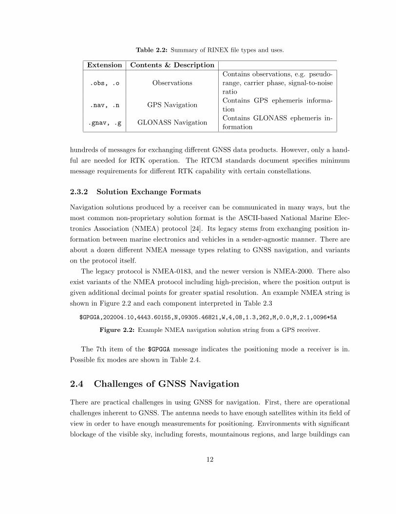
Table 2.2: Summary of RINEX file types and uses.

Extension Contents & Description

.obs, .o ObservationsContains observations, e.g. pseudo-range, carrier phase, signal-to-noiseratio

.nav, .n GPS NavigationContains GPS ephemeris informa-tion

.gnav, .g GLONASS NavigationContains GLONASS ephemeris in-formation

hundreds of messages for exchanging different GNSS data products. However, only a hand-

ful are needed for RTK operation. The RTCM standards document specifies minimum

message requirements for different RTK capability with certain constellations.

2.3.2 Solution Exchange Formats

Navigation solutions produced by a receiver can be communicated in many ways, but the

most common non-proprietary solution format is the ASCII-based National Marine Elec-

tronics Association (NMEA) protocol [24]. Its legacy stems from exchanging position in-

formation between marine electronics and vehicles in a sender-agnostic manner. There are

about a dozen different NMEA message types relating to GNSS navigation, and variants

on the protocol itself.

The legacy protocol is NMEA-0183, and the newer version is NMEA-2000. There also

exist variants of the NMEA protocol including high-precision, where the position output is

given additional decimal points for greater spatial resolution. An example NMEA string is

shown in Figure 2.2 and each component interpreted in Table 2.3

$GPGGA,202004.10,4443.60155,N,09305.46821,W,4,08,1.3,262,M,0.0,M,2.1,0096*5A

Figure 2.2: Example NMEA navigation solution string from a GPS receiver.

The 7th item of the $GPGGA message indicates the positioning mode a receiver is in.

Possible fix modes are shown in Table 2.4.

2.4 Challenges of GNSS Navigation

There are practical challenges in using GNSS for navigation. First, there are operational

challenges inherent to GNSS. The antenna needs to have enough satellites within its field of

view in order to have enough measurements for positioning. Environments with significant

blockage of the visible sky, including forests, mountainous regions, and large buildings can

12

Table 2.3: Dissection of the NMEA string above.

Item Portion Meaning

1 $GPGGA NMEA Header. GP means GPS-only, GGA is fix information.2 202004.10 GPS Time Of Day (20:20:04.10 UTC)3 4443.60155 Signless Latitude (44.4436015512 degrees)4 N Latitude North/South Indicator5 09305.46821 Signless Longitude (93.054682140 degrees)6 W Longitude East/West Indicator7 4 Fix Type (4 is RTK Fixed-Integer)8 08 Number of Satellites Used For Solution9 1.3 Horizontal Dilution of Precision10 262 Altitude of Antenna Above Sea-Level11 M Units of Altitude (Meters)12 0.0 Separation of Mean Sea Level and WG84 Geoid13 M Units of Separation (Meters)14 2.1 Age of Differential Corrections (seconds)15 0096 Reference Station ID16 *5A Checksum for Message Integrity

Table 2.4: Possible values for the GGA fix type.

Fix Type Solution Mode Description

0 No Fix Insufficient measurements to create a fix.1 2D Fix Horizontal position fix.2 3D Fix Horizontal and vertical position fix.3 DGPS Fix Differential pseudorange position solution.4 RTK Fixed-Integer Fixed-integer position solution.5 RTK Floating-Point Floating-point position solution.

prohibit GNSS operation. An active area of research involves ubiquitous navigation in urban

canyons using novel multipath detection and mitigation methods [25] and navigation using

other signal sources such as cellular or WiFi networks (also called signal-of-opportunity

navigation) [26].

There is also the risk of intentional interference that will prevent navigation. GNSS

interference detection and mitigation has motivated the continued development of GNSS

with more advanced cryptographic protections.

Other challenges for implementing GNSS navigation are the size and cost of the necessary

hardware and software. There are a wide variety of GNSS receivers, antennas, accessories,

and software solutions that range from the enterprise to the open-source options. Receivers

that can perform standard positioning are widely available and embedded in many consumer

devices, and RTK-capable receivers have been used in surveying equipment and specialized

autonomous vehicles since the late 1990s. Such specialized receivers come with a price tag in

13

excess of $10,000 and have proven reliability. Over the past several years, low-cost ($500 or

less) RTK-capable receivers have been introduced to the navigation marketplace. However,

these receivers are released and go obsolete quickly, leaving questions about their reliability

and performance in navigation applications. This growth of low-cost, RTK-capable GNSS

receivers prompted the assessment that is described in the next chapter.

14

3. Assessment

3.1 Introduction

As discussed previously, the implementation of RTK GNSS receivers has significant chal-

lenges and rewards. RTK operation requires a steady, constant stream of data from another

receiver and solving the integer ambiguity problem is no small feat. Once the problem is

solved, position solutions with centimeter level accuracy are realized and applications re-

quiring such accuracy are enabled. Historically, receivers capable of generating an RTK

solution that is both accurate and reliable were costly (in excess of $10,000) making them

unsuitable for cost-sensitive applications requiring high accuracy positioning. Additionally,

many early RTK corrections sources were proprietary and accessible with paid subscriptions

limited to certain hardware. Such is the case with the John Deere RTK network (which

only works with John Deere affiliated receivers) [27].

A CORS network is a number of stationary GNSS receivers distributed across a geo-

graphic area that provide RTK-enabling data on a continuous basis. The primary method

for accessing a CORS network is the internet using the NTRIP (Networked RTK over Inter-

net Protocol) architecture [28]. Recently, more receivers have built-in NTRIP support and

many clients are available for accessing data. The Minnesota Continuously Operating Refer-

ence Station (MnCORS) network operated by the Minnesota Department of Transportation

(MnDOT) is a service available to the public free of charge [29].

Recently, GNSS equipment manufacturers have started advertising inexpensive (less

than $1,000) RTK-capable receivers that can use Continuously Operating Reference Station

(CORS) networks. The cost of these receivers is much lower than traditional receivers. The

assessment described in this chapter was motivated by the unknown performance of low-

cost, RTK-capable GNSS receivers using a CORS network.

The first motivation for this assessment was to aid in the development and evolution of

the Minnesota Continuously Operating Reference Station (MnCORS) network operated by

the Minnesota Department of Transportation (MnDOT). A map of the MnCORS network

is shown in Figure 3.1. If new RTK-capable receivers can provide centimeter-level accuracy

inexpensively, it may lead to a surge in the user base demanding access to the MnCORS

network.

The second motivation for this work stems from on-vehicle applications. Autonomous

vehicles and other intelligent transportation systems are one consumer of GNSS systems

requiring positioning at the centimeter level [30]. For example, one application is using

GNSS paired with high-accuracy maps to determine a vehicle’s relative position within the

15

road geometry. This method is particularly useful when navigating in environments where

weather may degrade the performance of other sensors such as in a blizzard. Ensuring

system performance in these environments drives the need for GNSS-based solutions that

can increase system robustness and reliability. If low cost receivers can provide sufficient

performance, this may enable a level of ubiquity not currently feasible for automated vehicle

applications.

Next, the performance metrics that governed this assessment are discussed. These

metrics cover most aspects of receiver performance as it relates to reliable navigation, though

not all.

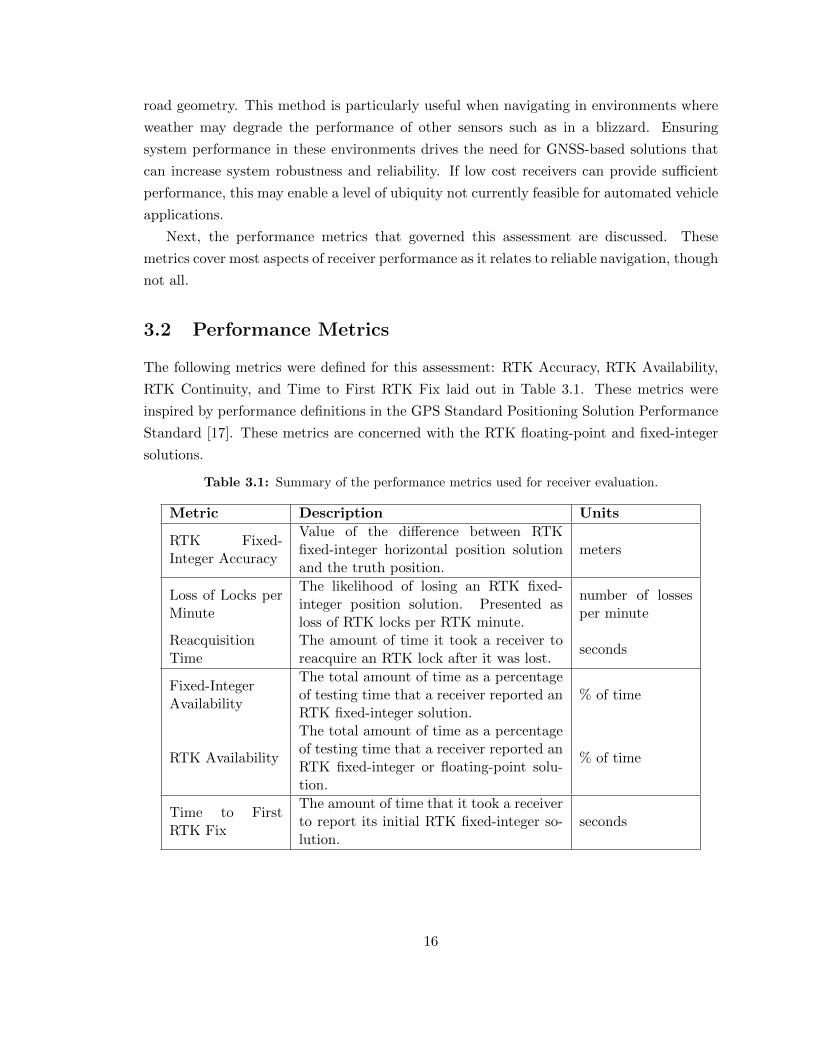
3.2 Performance Metrics

The following metrics were defined for this assessment: RTK Accuracy, RTK Availability,

RTK Continuity, and Time to First RTK Fix laid out in Table 3.1. These metrics were

inspired by performance definitions in the GPS Standard Positioning Solution Performance

Standard [17]. These metrics are concerned with the RTK floating-point and fixed-integer

solutions.

Table 3.1: Summary of the performance metrics used for receiver evaluation.

Metric Description Units

RTK Fixed-Integer Accuracy

Value of the difference between RTKfixed-integer horizontal position solutionand the truth position.

meters

Loss of Locks perMinute

The likelihood of losing an RTK fixed-integer position solution. Presented asloss of RTK locks per RTK minute.

number of lossesper minute

ReacquisitionTime

The amount of time it took a receiver toreacquire an RTK lock after it was lost.

seconds

Fixed-IntegerAvailability

The total amount of time as a percentageof testing time that a receiver reported anRTK fixed-integer solution.

% of time

RTK Availability

The total amount of time as a percentageof testing time that a receiver reported anRTK fixed-integer or floating-point solu-tion.

% of time

Time to FirstRTK Fix

The amount of time that it took a receiverto report its initial RTK fixed-integer so-lution.

seconds

16

3.2.1 RTK Accuracy

In general, GNSS accuracy is defined as the difference of the calculated position error and

the truth position that is exceeded only 5% of the time in the absence of system errors [11].

Stated another way, this is the 95th percentile of the position errors. The RTK Fixed-Integer

Accuracy is calculated using the difference between a receiver’s RTK position solution and

a truth position. After an ensemble of position solutions are collected, the position errors

are used to create an empirical cumulative distribution function.

3.2.2 RTK Availability

The RTK Availability is defined as the total amount of time that a receiver spends in RTK

mode, broken down into fixed-integer and floating-point modes. An ideal receiver would

have a fixed-integer availability close to 100%.

3.2.3 RTK Continuity

The formal definition of continuity is the likelihood of a detected but unscheduled navigation

function interruption after an operation has been initiated [17]. Once a receiver has com-

puted an RTK fixed-integer solution, it may lose the solution and fall back to floating-point

mode.

Two values are used for the RTK Continuity metric. The first is Loss of Locks per

Minute, which is the number of times a receiver falls out of RTK fixed-integer mode divided

by the total amount of time it spent in RTK fixed-integer mode. The second is Reacquisition

Time, which is the time it took a receiver to reacquire the fixed-integer solution after losing

it.

3.2.4 Time to First RTK Fix

The time to first fix (TTFF) is a performance metric of receiver initialization. It is the

amount of time that it takes to report a solution from a cold start (no knowledge left over

from its previous operational state). The Time to First RTK Fix is the amount of time a

receiver takes to report its initial RTK fixed-integer solution.

3.3 Experiment Setup

The key criteria for selecting a receiver was a price of ∼$500 or less and advertised RTK

positioning capability using a CORS network. The selected receivers are not representative

of all possible choices. Table 3.2 provides an overview of all the receivers. The Hemisphere

Eclipse P307 was included at the request of MnDOT due to the agency’s ongoing use of the

17

receiver. Though it is a mid-range receiver in terms of cost (greater than $1000), it is still

a more affordable option compared to the most expensive receivers.

Two antennas were used: a multifrequency antenna and a single-frequency patch an-

tenna. The multifrequency antenna was a Navcom ANT-3001R antenna with an LNA gain

of 39 dB [31]. The patch antenna was an ANN-MS L1-only antenna with an LNA gain of

29 dB [32].

The receivers were connected to a single antenna through a GPS Technologies ALDCV1x8

signal splitter. They were connected to a laptop computer via USB that ran the data col-

lection software. The data collection software was a custom application built in Python.

RTK corrections data was provided by the MnCORS network. This service was accessed

over the internet by connecting the laptop to a cellular modem. Figure 3.2 shows a diagram

of the experimental setup.

The receiver output were National Marine Electronics Association (NMEA) strings, a

human-readable format used for reporting GNSS solutions. The type-GGA string contains

the latitude, longitude, position-fix type and other relevant information about the GPS

fix of the receiver [24]. Position errors were calculated using the Navpy [33] and Pynmea2

[34] Python packages. The RTK solutions were computed on the receiver and not in post-

processing.

The initial position calculated by a receiver was sent to the MnCORS network. The

MnCORS network uses the Virtual Reference Station (VRS) method to generate measure-

ments from a virtual base station near the initial position. The typical distance of the

virtual station the receiver, or baseline length, is a few meters [35]. MnCORS provides

GPS and GLONASS L1/L2 observations at a rate of 1 Hz. After a receiver calculated a

new position solution, it was sent to the MnCORS network again and the cycle repeated.

Table 3.2: Summary of the receivers used for this assessment.

Receiver Bands GNSS Price

Swift Piksi Multi L1/L2 GPS

<∼$500NVS TechnologiesNV08C-RTK

L1 GPS + GLO

Emlid Reach L1 GPS + GLOu-blox NEO-M8P L1 GPS + GLOSkytraq S2525F8-RTK

L1 GPS + GLO

HemisphereEclipse P307

L1/L2 GPS + GLO >$1000

18

3.3.1 PyRTK Data Collection Software

To run each receiver and respective MnCORS connections simultaneously, an application

was written in Python. A user specifies receivers and USB devices in XML files. An inter-

face was developed to communicate the navigation state of each receivers, basic diagnostic

information, and a field to specify the amount of time to collect data for. After pressing

the Start button, the program would begin to search for each receiver’s USB device name.

One low-cost receiver, the Skytraq S2525F8-RTK, used a separate input and output

USB port for sending and receiving data. However, the USB devices were identical from

a software perspective, so a serial watchdog was used to determine which port was which

when the experiment began. The first serial port to send out NMEA strings was considered

the output port and the other the input port. The software is stored in a GitHub repository

at [36].

3.3.2 Static Test Considerations

Static testing was conducted using geodetic monuments as truth positions. The antenna

was mounted on a constant-height tripod placed over the monument. Three monuments,

named TURKEY MN037, UNIVERSITY1934 and SCHREIBER, were chosen to best reflect

the qualitative characteristics of rural, suburban and urban settings respectively. The rural

marker was located near farmland at UMore Park, the UNIVERSITY1934 marker was on

the University of Minnesota, Twin Cities campus, and the SCHREIBER marker was located

northwest of the University of Minnesota. Figures showing the location of these markers are

available in the Appendix. They were found using MnDOT’s interactive geodetic monument

viewer [37]. The chosen test sites were a compromise in the availability of markers and

desired features. All static data was collected in 25-minute-long sessions on 17 days over

4 months. The data was collected roughly at the same time of day, though it was not a

priority to have the same satellites in view.

3.3.3 Dynamic Test Considerations

The dynamic tests were conducted using a vehicle outfitted with the Navcom ANT-3001R

multifrequency antenna. A Navcom SF-3050 receiver was used to provide truth positions

to calculate receiver accuracy. The Navcom was chosen due to its favorable operating

characteristics. It has an RTK RMS accuracy of 1 cm + 1 ppm, a quick RTK initialization

time, and is designed for dynamic applications [38]. The ANN-MS patch antenna was

omitted from the dynamic testing because of its incompatibility with the SF-3050 receiver.

Three routes were chosen for the dynamic testing to represent different environments.

The urban route ran through downtown St. Paul and Minneapolis through the Lowry Hill

19

tunnel along interstate 94. The rural route followed Neal Ave. South from Hudson Rd.

South to 122nd Ave. South in Woodbury, MN. The last route was a highway with overhead

bridges that ran from Neal Ave. South along I-94 to 122nd Ave. South via highway US 10.

At the beginning of each data collection session, the vehicle was idled for five minutes for the

receivers to initialize. Each route took about 20 minutes to drive and was repeated traveling

in the opposite direction e.g. northbound and southbound. Each route was repeated six

times. A map of each route is available in the Appendix.

3.4 Static Experiment Results

3.4.1 Accuracy for Static Tests

Accuracy is presented as an empirical cumulative distribution function (CDF) between the

50th and 95th percentiles for the multifrequency and patch antennas. CDFs are a useful

for understanding the probability distribution of a random variable, and receiver accuracy

is often cited with respect to a certain percentile e.g. 50-percent accuracy [39].

Accuracy CDFs from the rural location are seen in Figure 3.4 and Figure 3.5. The

results in the rural environment can be considered the best-case scenario. All of the low-

cost receivers have 5 cm accuracy up to the 75th percentile while using the multifrequency

antenna. The Eclipse P307 and Piksi Multi maintain 5 cm accuracy or better up to the

95th percentile using the multifrequency antenna. Using the patch antenna, the Eclipse

P307, Reach, and NEO-M8P maintain 5 cm accuracy up to the 95th percentile. This is the

only experiment where the Reach and NEO-M8P did not exhibit accuracy degradation.

In Figure 3.4, a large jump in the error magnitude can be seen for a couple of receivers

after the 68th percentile. This large jump is approximately the wavelength of a single L1

GPS cycle, 19 centimeters. These accuracy degradations are likely due to the receivers

using an incorrect integer to calculate the position solution. This behavior can be seen in

many other figures, and highlights the effects of choosing incorrect integers.

Accuracy CDFs from the suburban location are presented in Figure 3.6 and Figure 3.7.

Using the multifrequency antenna, only the Eclipse P307 maintains centimeter-level accu-

racy up to the 95th percentile. Only the Reach and Eclipse P307 maintain centimeter-level

accuracy up to the 95th percentile using the patch antenna.

Accuracy CDFs from the urban location are presented in Figure 3.8 and Figure 3.9. Us-

ing the multifrequency antenna, only the Reach and Eclipse P307 maintains centimeter-level

accuracy up to the 95th percentile. Using the patch antenna, many receivers exhibit accu-

racy degradation well before the 50th percentile, evident by the Piksi Multi, S2525F8-RTK

and NV08C-RTK receivers in Figure 3.9. Only the Eclipse P307 maintained centimeter-level

accuracy up to the 95th percentile.

20

Figure 3.1: Map of the Minnesota Continuously Operating Reference Station (MnCORS) network.

21

Figure 3.2: Illustration of the experimental setup.

Figure 3.3: The hardware setup showing the low-cost receivers in a protective container.

22

Figure 3.4: Horizontal position accuracy CDF from static testing at the rural location using themultifrequency antenna.

23

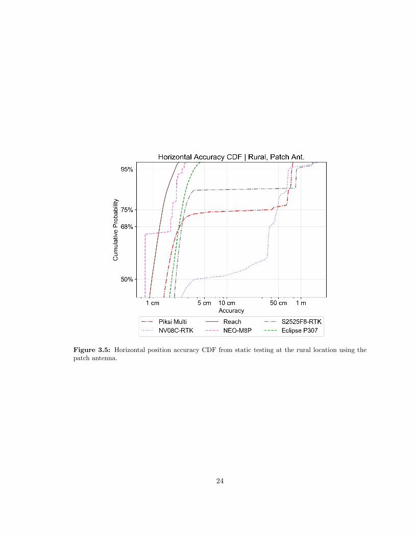
Figure 3.5: Horizontal position accuracy CDF from static testing at the rural location using thepatch antenna.

24

Figure 3.6: Horizontal position accuracy CDF from static testing at the suburban location usingthe multifrequency antenna.

25

Figure 3.7: Horizontal position accuracy CDF from static testing at the suburban location usingthe patch antenna.

26

Figure 3.8: Horizontal position accuracy CDF from static testing at the urban location using themultifrequency antenna.

27

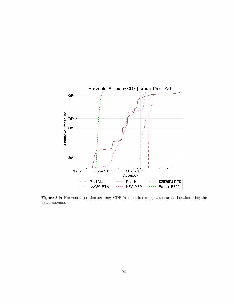
Figure 3.9: Horizontal position accuracy CDF from static testing at the urban location using thepatch antenna.

28

3.4.2 Availability for Static Tests

The total percentage of time that a receiver spent in RTK fixed-integer or floating-point

mode are shown in Figure 3.10, Figure 3.11 and Figure 3.12 for each environment. Nearly

all the receivers spent more time in RTK fixed-integer mode in the rural location regardless

of antenna choice. The worst availability was observed in the urban environment.

The antenna had a clear effect on the availability of the multifrequency receivers, the

Eclipse P307 and the Piksi Multi. Using the multifrequency antenna, both receivers reported

an RTK fixed-integer position more than 95% of the time. However, the availability drops

off when the patch antenna was used.

This relationship was less prominent for the single-frequency receivers. In the rural

environment, the RTK availability for the single-frequency receivers is nearly the same re-

gardless of antenna. In the suburban and urban environments, the multifrequency antenna

more often results in a higher RTK availability. This could be a result of the build qual-

ity, the higher signal gain, or phase-center stability characteristics of the multifrequency

antenna.

Figure 3.10: RTK availability for static testing in the rural environment. The darker color denotesfixed-integer mode and the lighter color floating-point mode.

29

Figure 3.11: RTK availability for static testing in the suburban environment. The darker colordenotes fixed-integer mode and the lighter color floating-point mode.

30

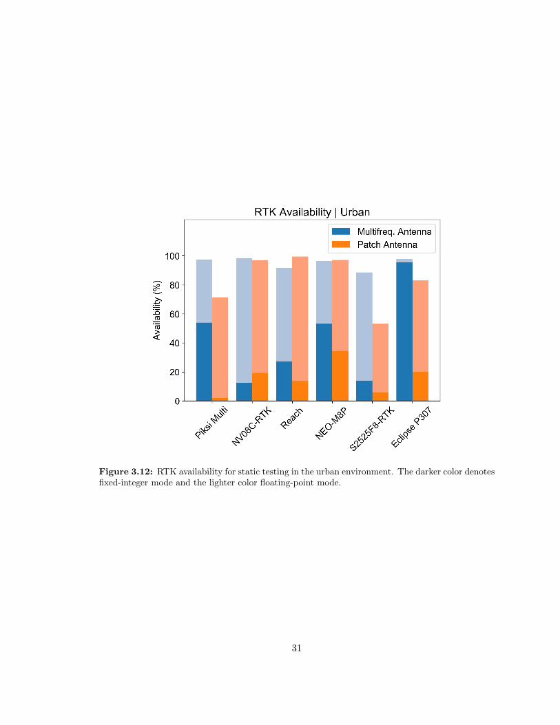
Figure 3.12: RTK availability for static testing in the urban environment. The darker color denotesfixed-integer mode and the lighter color floating-point mode.

31

3.4.3 Continuity for Static Tests

The receivers’ loss of lock averages are shown in Table 3.3. Except for the NV08C-RTK

and S2525F8-RTK, there was a dependence on environment and the average number of

losses. In the rural environment, a receiver was less likely to lose an RTK lock. Using

the multifrequency antenna, a receiver was less likely to experience a loss of lock. The

S2525F8-RTK and NV08C-RTK were prone to higher RTK fixed-integer lock losses in all

environments.

The average times to reacquire the RTK fixed-integer solution are shown in Table 3.4.

Using the patch antenna resulted in some cases where RTK fixed-integer was lost and reac-

quisition did not take place within the experimental time of 25 minutes, such as the Eclipse

P307 in the rural and urban environments. This is not to say that it would not reacquire

the RTK fixed-integer solution ever. In the rural environment, the multifrequency antenna

usually led to quicker RTK reacquisition times. In the other environments, there is no clear

relationship between antenna quality and the RTK reacquisition time. Curiously, the Piksi

Multi reported a reacquisition time greater than 800 seconds in the suburban environment

using the multifrequency antenna. It reported an RTK fixed-integer reacquisition time in

only two of the tests using the multifrequency antenna and is likely related to its robustness

in operating in challenging environments.

Table 3.3: RTK Losses per RTK Minute in the (R)ural, (S)uburban and (U)rban environmentsfrom static testing.

ReceiverMultifreq. Antenna Patch AntennaR S U R S U

Piksi Multi 0.03 0.03 0.11 0.04 0.93 0.86NV08C-RTK 0.73 11.04 11.66 13.74 1.95 2.27Reach 0.07 4.43 1.55 0.13 10.53 2.18NEO-M8P 0.03 0.86 0.48 0.09 1.02 3.79S2525F8-RTK 8.24 7.4 9.22 0.72 4.68 0.16

Eclipse P307 0.09 0.03 0.03 0.02 0.11 0.04

3.4.4 Time to First RTK Fix

The average times to first RTK fix are shown in Table 3.5. The time to acquire an RTK

solution is dependent on the quality of the received signals (which is affected by propagation

errors as well as antenna phase center motion), whether or not the receiver is multifrequency,

and the algorithms built into the firmware.

Unsurprisingly, there is a clear benefit to using the multifrequency antenna with the

multifrequency receivers. By using two or more frequencies, a receiver has double or greater

32

Table 3.4: RTK Reacquisition Time (seconds) in the (R)ural, (S)uburban and (U)rban environ-ments from static testing.


Piksi Multi 8 853 150 410 110 *NV08C-RTK 13 19 22 18 29 10Reach 74 84 202 161 20 97NEO-M8P 66 233 194 74 351 211S2525F8-RTK 299 172 210 262 197 624

Eclipse P307 4 18 31 * 812 *

the information at hand which makes RTK initialization quicker. This benefit is lost when

using the single-frequency patch antenna.

Table 3.5: Time (seconds) to Initialize RTK Fixed-Integer solution and hold for 10 subsequentseconds in the (R)ural, (S)uburban and (U)rban environments from static testing.


Piksi Multi 76 260 491 411 311 827NV08C-RTK 551 290 445 294 697 170Reach 465 332 643 393 226 366NEO-M8P 307 337 407 294 537 356S2525F8-RTK 901 1887 936 684 913 1528

Eclipse P307 52 61 62 607 749 818

3.5 Dynamic Experiment Results

In the figures that follow each bar color represents a different location (left to right): red

for the rural route, brown for the bridges route, and purple for the urban route.

3.5.1 Accuracy for Dynamic Tests

The horizontal accuracy CDFs of the fixed-integer solutions are shown in Figure 3.13,

Figure 3.14, and Figure 3.15 for each environment. The multifrequency receivers maintained

an accuracy of 16 cm (95%) or better on all routes. The Reach maintained accuracies of

2 cm (95%) on the suburban and urban routes and NEO-M8P had an accuracy of 15 cm

(95%) on the bridges route. At the 50th and 68th percentiles, the accuracy of most receivers

is 10 cm or better. Up to the 95th percentile, many receivers errors diverge towards 1+

meters.

33

Figure 3.13: Horizontal position accuracy CDF from dynamic testing on the rural route using themultifrequency antenna.

34

Figure 3.14: Horizontal position accuracy CDF from dynamic testing on the overhead bridgesroute using the multifrequency antenna.

35

Figure 3.15: Horizontal position accuracy CDF from dynamic testing on the urban route usingthe multifrequency antenna.

36

3.5.2 Continuity for Dynamic Tests

The route with bridges running along US-10 in St. Paul was specifically chosen to explore

the RTK fixed-integer loss and reacquisition time when traveling under bridges. The only

receivers that had an RTK fixed-integer lock consistent enough to evaluate the effects of

bridges were the Piksi Multi and Eclipse P307. These receivers have the same mean loss of

RTK instances in the bridges route.

There was no distinction made in the data between a loss of RTK due to bridges or a

different cause e.g. a hauling truck or a retaining wall. However, Figure 3.16 and Figure 3.17

show a portion of the bridge route where the test vehicle drove under a bridge. The Eclipse

P307 fell into an RTK floating-point solution almost immediately, then reacquired the RTK

fixed-integer solution 19 seconds later. The Piksi Multi completely lost its RTK solution

after traveling under a bridge and took about 41 seconds to reacquire an RTK fixed-integer

solution.

Figure 3.16: Piksi Multi RTK fixed-integer loss of lock while traveling under a bridge on theoverhead bridges route. RTK fixed-integer (green), RTK floating-point (orange), standard positionfix (red).

37

Figure 3.17: Eclipse P307 RTK fixed-integer loss of lock while traveling under a bridge on theoverhead bridges route. RTK fixed-integer (green), RTK floating-point (orange), standard positionfix (red).

38

3.5.3 Availability for Dynamic Tests

The RTK availability for each receiver is shown in Figure 3.18. The availability of the RTK

fixed-integer solution was much lower for all receivers in the dynamic case than the static

case. The single-frequency receiver with the best fixed-integer availability of 27% was the

NEO-M8P on the rural route. When both RTK fixed-integer and floating-point solutions

were considered, all the receivers perform similarly. The Piksi Multi and Eclipse P307 had

similar RTK fixed-integer availability on all routes. The multifrequency receivers overall

had a higher availability, with the worst-case of the Piksi Multi in the urban environment

outperforming all of the single-frequency receivers.

Figure 3.18: RTK availability from dynamic testing for each route using the multifrequency an-tenna. The darker color denotes fixed-integer mode and the lighter color floating-point mode.

39

3.6 Discussion

Of the low-cost receivers tested, the Piksi Multi exhibited the best performance while using

the multifrequency antenna. It had consistent accuracy and higher availability in all envi-

ronments during static and dynamic testing. The NEO-M8P and Reach receivers performed

similarly during most tests, static and dynamic, with some exceptions. The NV08C-RTK

and S2525F8-RTK displayed the worst metrics in both from both the static and dynamic

tests in all environments.

Even the Piksi Multi fell short of the performance of the mid-range Eclipse P307 that had

unparalleled consistency in all environments during the static and dynamic tests. However,

this advantage is limited only to when the Eclipse P307 is using the multifrequency antenna,

as its metrics degrade substantially using the patch antenna. This highlights the importance

of using a multifrequency antenna with a multifrequency-capable receiver.

The single-frequency, L1-only low-cost receivers excelled with respect to one metric but

performed poorly relative to others. Though a few had CDF curves that were stable up to

the 90th percentile, they were marred by their poor availability and continuity character-

istics especially in the suburban and urban environments. The following observations are

made about the single frequency receivers evaluated in this work:

1. They all achieved centimeter-level accuracy (95%) during static tests in the rural

environment.

2. The metrics did not heavily depend on the use of the L1-only or L1/L2 antenna.

3. All metrics degraded when testing in the urban and suburban environments.

4. When not in fixed-integer mode, they spent most of their time in floating-point mode.

5. Absolute fixed-integer availability fell during dynamic tests, but relative availability

was consistent.

During the static tests, the low-cost receivers had nominal performance in the rural

environment where there was minimal signal interference. Three of the five low-cost receivers

had a horizontal RTK fixed-integer position accuracy of 2.6 cm (95%) or better while the

other two had sub-meter accuracy. In the rural environment, the L1-only receivers had

lower RTK availability and initialization times compared to the multifrequency receivers.

The Emlid Reach and u-blox NEO-M8P maintained a sub-5cm accuracy (95%) accuracy

in the rural environment using the patch antenna. Per Table 3.3, both had stable RTK

fixed-integer solutions with loss-lock averages of less than 0.2 lock losses per RTK-minute.

Both receivers had similar RTK fixed-integer availability metrics seen in Figure 3.10.

40

The suburban and urban environments had a negative impact on the RTK fixed-integer

accuracy of the low-cost receivers. These are environments replete with interference that

introduce error into the measured signals, as expected. These challenges are minimized in

the open-sky, rural environment. Methods exist for multipath detection and mitigation [40]

and are employed by some receivers such as the Eclipse P307, which maintained centimeter-

level accuracy metrics across all testing environments. The effects are evident in Figure 3.8

and Figure 3.9. Using the multifrequency antenna, most receivers have 5 cm accuracy up to

the 60th percentile until errors become more pronounced. Using the patch antenna, most

receivers have accuracy values worse than 10 cm at the 50th percentile.

The multifrequency Piksi Multi displayed the same shortcomings (degraded accuracy,

worse availability) in the suburban and urban environments during static testing. In the

rural environment, it had an availability above 95% and a stable CDF curve that paralleled

the Eclipse P307. Using the multifrequency antenna, it had a very stable RTK fixed integer

solution with an average of 0.03 fixed-integer losses per minute in the rural and suburban

environments and 0.11 losses per minute in the urban environment.

During the dynamic tests, the L1-only receivers had low RTK fixed-integer availability

and continuity. Although the absolute RTK fixed-integer availability was lower during

dynamic tests, the relative availability between each receiver stayed the same. This is

evident by comparing say Figure 3.10 and Figure 3.18. In addition, some receivers had

large position errors that exceeded 1 meter. Although not presented here, some of the

L1-only receivers had floating-point solution errors on the order of hundreds of meters and

kilometers.

The low-cost Piksi Multi had higher RTK availability and maintained stable accuracy

up to the 95th percentile (relative to the Navcom receiver) during on-vehicle testing com-

pared to the low-cost, L1-only receivers. There’s an obvious benefit to having additional

information at the ready for positioning in the dynamic environment. The continuity anal-

ysis of the Piksi Multi showed reacquisition times greater than 40 seconds after traveling

underneath a bridge. Such long reacquisition times may be prohibitive for certain on-vehicle

applications.

The Eclipse P307 maintained consistent accuracy, availability and continuity statistics

in all environments using the multifrequency antenna. It was also capable of operating

with the L1-only antenna, though its availability, continuity and initialization degraded as

a result. It also showed accuracy degradation using the patch antenna in some cases. While

its performance metrics were better than the low-cost receivers’, it comes at a price that

could be prohibitive for mass-market applications.

The receiver firmware used in this assessment are listed in Table 3.6 and were current as

of March 2017. There have been a couple of notable updates for the Piksi Multi, including

41

an update that introduces support for the GLONASS constellation. Future work could

quantify the changes in receiver performance of new firmware.

Table 3.6: Firmware loaded on each receiver used in this assessment.

Receiver Firmware Version

Swift Piksi Multi 1.1.27NVS Technologies NV08C-RTK V0029Emlid Reach 2.3u-blox NEO-M8P HPG 1.20REFSkytraq S2525F8-RTK NS-HP-GL-10S (20170712)

3.7 Conclusion

A black-box assessment of five low-cost, RTK-capable GNSS receivers was performed for

MnDOT investigating multiple performance metrics. This assessment provided insight into

the built-in RTK capability of each receiver in static and dynamic scenarios using a CORS

network. Of the low-cost receivers, the multifrequency Swift Piksi Multi had the most

stable accuracy, highest availability and a stable fixed-integer solution while using the mul-

tifrequency antenna. All low-cost receivers exhibited degraded metrics in environments

with obstructed sky view, though the mid-range receiver was consistent in the other en-

vironments. Accuracy and availability were degraded for all receivers during the dynamic

testing, but relative receiver performance was consistent. The mid-range Eclipse P307 re-

ceiver outperformed all of the low-cost receivers in static and dynamic testing, but is an

order of magnitude more expensive than the low-cost receivers (but more affordable than

the $10,000+ high-end receivers, too).

In the end, a user needs to weigh the performance metrics that are important for their

application and choose a receiver accordingly. It is reasonable to anticipate that low-cost,

RTK receivers will become more robust and capable in the future, and in fact, u-blox

recently announced a new low-cost, multifrequency chipset [41]. I’s likely that many of the

low-cost receivers would perform better with firmware updates. Of interest is the Piksi

Multi which introduced GLONASS support after testing had begun. This assessment is a

starting point for future assessments of new, low-cost RTK receivers.

42

4. Forecasting

4.1 Introduction

Performing RTK navigation requires a steady stream of data from an a reference receiver.

This can come from a CORS network accessed via the internet or a second receiver via

a very high frequency (VHF) radio. A reliable connection between the rover receiver and

the reference receiver is needed to maintain RTK operation. Unless the two receivers are

physically connected, as in the case of using two receivers for heading determination, a user

runs the risk of losing the RTK position if the connection degrades or is completely lost.

For a brief period, a receiver can use old data for RTK positioning if there is latency in

the connection. A variable known as the age of differential corrections is used to commu-

nicate the age, in seconds, of the most recent data from the RTK data source. The age of

differential corrections begins increasing when a receiver does not receive new RTK data.

Many receivers will cease RTK navigation if the age of differential corrections grows too

large A typical threshold is thirty seconds. Performing navigation with differential correc-

tions data that is older than this results in growing position solution errors. After ceasing

RTK navigation, a receiver will report the standard (code-phase) position solution until

they receive new corrections.

Operating RTK receivers in the field can result in increased latency and loss of a con-

nection with a corrections source. If the source is a CORS network accessed via a cellular

internet connection, performance will be worse in areas with poorer cellular network cov-

erage. Many rural regions still lack reliable cell service. Internet access with satellites can

be interrupted by atmospheric disturbances and is not as ubiquitous as cellular access. A

hard-wired internet connection is impractical or impossible for a receiver that is operating

on a vehicle or in a remote, natural location.

Vehicles that use GNSS navigation often employ an inertial navigation system (INS)

in conjunction with GNSS to bridge the gap when receivers lose position lock [42]. These

systems, called GNSS/INS or GPS/INS filters, are only useful for short-term solutions

unless expensive, tactical-grade sensors are employed. One study used RTK GPS and INS

on transit buses for bridge-induced RTK fixed-integer losses with an average length of 10

seconds [43]. The resulting GNSS/INS filter was capable of producing position solutions

with mean position errors on the order of centimeters during the RTK outages. While

effective in the short-term, the position solution errors will diverge with time unless the

fixed-integer solution is regained.

To mitigate these challenges, this chapter explores the concept of using a recurrent neural

43

Figure 4.1: Overview of forecasting architecture.

network (RNN) time-series forecaster to predict differential corrections based on older data

received. As RTK navigation becomes incorporated into autonomous technologies that

operate on roadways and in airspace, creating solutions to make positioning more robust

will increase the safety of these systems, which will lend themselves to be adopted more.

Most modern RTK applications revolve around surveying and farm equipment navigation,

but its use in autonomous vehicle navigation both in the ground and the air is increasing.

Novel uses for RTK navigation include autonomous search and rescue missions, unmanned

aerial vehicle package deliveries, automatic close-point infrastructure inspection, and direct

georeferencing of agriculture and structural assets. Any mission that uses RTK navigation

would benefit from increased robustness against corrections data loss.

The motivation for choosing this problem stemmed from the hands-on experience with

the hardware described in the last chapter. There were portions of the dynamic test when

the cellular connection was lost, resulting in every receiver being tested to fall out of RTK

navigation mode only to pick it up again seconds later. The focus on an RNN-based

approach was a matter of interest in the subject. RNN architectures have been applied to

interesting problems, such as generating Wikipedia articles [44] and learning to play arcade

video games [45]. In each application, the problem is broken down into a sequence of inputs

and a response to said inputs.

The architecture for an RNN forecaster for RTK corrections data is illustrated in Fig-

ure 4.1. The hardware components of the system are an RTK-capable GNSS receiver and

antenna, a computer, and connection hardware for the external corrections data e.g. a cel-

lular modem for accessing a CORS network. The software components are few; first, there

is an RNN forecaster that is trained on the corrections data. Second, there is a monitor that

requests forecasts from the RNN in case the external corrections data is lost for a period

of time. To the receiver, it will seem as though the connection to the external source has

been maintained. If the connection with the external source is revived, the monitor would

continue to train the RNN forecaster and send the external data to the receiver. If the

connection is lost for too long, the system will stop sending data altogether to the receiver

as forecast errors tend to grow the farther the horizon. The receiver will go into single

44

point positioning mode, and the centimeter and decimeter-level accuracy will be lost. This

envisioned architecture for the RNN-based forecaster is a stop-gap measure for maintaining

centimeter-level accuracy in case of temporary external corrections data loss.

This leads to questions that were asked for this project:

1. Can an RNN-based forecaster be used to generate RTK-quality forecasts given a time-

series of corrections data?

2. If yes, how long is the effective forecasting horizon of such a forecaster?

This project has not fully answered the above questions. Rather, it has been an exer-

cise in answering the first question by experimenting with different network architectures

and input-output schemes. The strategies outlined in this chapter fall short of creating

centimeter-level position solutions using forecasted data but are a stepping stone for future

study.

Similar techniques have been demonstrated for time-series forecasting, even in the realm

of differential GPS. The following sections review work related to differential GPS fore-

casting neural networks, a brief introduction to neural networks, and the details of the

experiments carried out.

4.2 Related Work

Neural networks combined with an unscented Kalman filter have been studied to perform

online prediction of pseudorange correction values for DGPS using a 2-hour dataset [46].

The neural network was trained online using the ten previous inputs while looking ahead

one, five and ten timesteps. The results from only two satellites are presented, and the

longest complete outage considered was 10 seconds.

Artificial neural networks have been used to bound Autoregressive Moving Average

(ARMA) and Autoregressive (AR) models of different orders [47]. The models were used

to predict pseudorange and carrier phase corrections for DGPS predictions. Experiments

they conducted showed a 6.691 meter position accuracy (95%) with DGPS outages and

no predictions and 2.553 meter accuracy (95%) with predictions using the ARMA and AR

neural networks. Their networks were capable of forecasting usable DGPS products for

18-20 seconds before the forecasts diverged and become unusable.

The efficacy of different dynamic neural networks in predicting pseudorange corrections

for several satellite vehicles have been compared [48]. In these experiments, neural networks

with time delays, non-linear autoregressive, and recurrent architectures were trained on a

dataset, and then validated by forecasting the same dataset. The best performing network

in their experiments was the Layer Recurrent Neural Network (LRNN), though it is likely

45

that the LRNN memorized the data and has limited capability for forecasting data beyond

what it was trained on.

4.3 Neural Network Background

The idea of neural computation was discussed in 1943, when McCulloh and Pitts explored

modeling biological neural activity [49]. The basis of their formulation was the concept

of neuron excitation, that a neuron was either “on or off”. For a neuron to be excited, a

minimum number of the neuron’s neighbors must be excited and the neuron without an in-

hibitor. Also, the structure of the overall network does not change over time. This structure

of connected neurons and their interactions gave rise to the artificial neural network, which

has proliferated the areas of artificial intelligence, computation and estimation, control, and

many other sectors of technology and science.

In the modern sense, the basic component of a neural network is referred to as a neuron,

unit or node. A neuron is modeled as a nonlinear function with an input x and output h.

The parameters governing the structure of the neuron are the input weights w, the bias

b, and the activation function F illustrated in Figure 4.2. The activation function F is a

non-linear function that is commonly a sigmoid function that has an “S” shape, though it

can also be a linear function, rectified linear function, or other functions that satisfy the

required activation behavior. The output of a neuron is given by

h = F (

N∑i=1

wixi + b) (4.1)

Figure 4.2: Illustration of a single neuron.Figure 4.3: Illustration of a 2-layer, fully-connected neural network [50].

46

A neural network is made of individual neurons connected in various ways. The data

being fed into a neural network, x = x1, x2, . . ., is called the input. The final layer of the

network y = y1, y2, . . . is called the output layer. Between the input and output layer are the

hidden layers h = h1, h2, . . ., called so for being sandwiched inbetween the aforementioned.

The number of hidden layers defines the depth of a neural network. A neural network

can contain any number of hidden layers, and each hidden layer can contain an arbitrary

number of neurons. Figure 4.3 illustrates the layer topology of a 2-layer, fully-connected

neural network, i.e. the output of every layer is used as the input to the subsequent layer.

The number of hidden layers, the number of units in each layer, and the size of the input

and output of a neural network is known as network topology. Topological parameters that

need to be specified for creating a neural network are the number of hidden layers, the

number of units (neurons) in each hidden layer, the activation function(s) for each layer

and the size of the input and output layer. The choice of topological parameters is a

combination of art and science. The black-box nature of neural networks leaves much

desired to be understood about the complexity of their structure.

4.3.1 Recurrent Neural Networks

In the above neural network architecture, the state of each hidden-layer neuron h is not

persisted in time. In the recurrent neural network (RNN) architecture, each hidden-layer

neuron state h at one epoch is used as an input in the next epoch. This introduces a

degree of state persistence that lends itself to problems related to time-series analysis, as

the internal state of the network incorporates a form of memory separate from the input

data. Figure 4.4 illustrates the recurrence between internal states hk, hk+1 and so on.

Figure 4.4: Graphic illustrating general recurrent neural network architecture.

The following two equations are the basis of a general RNN model [44]. These two

47

equations are iterated over each timestep t = 1, . . . , T . and layer n = 2, . . . , N in the RNN.

Beginning with the first layer,

h1t = H(Wh1xt +Wh1h1h

1t−1 + b1h) (4.2)

where H is the layer activation function and W is a matrix of weights for each dependence

for The output is dependent on the weighted input xt, the weighted output of the same

layer from the previous timestep t − 1, and the layer’s bias. The time recurrence can be

removed by setting Wh1h1 = 0, which is a standard neural network layer. The inter-layer

recurrence is modeled by

hnt = H(Whnxt +Whn−1hnhn−1t +Whnhnh

nt−1 + b1h) (4.3)

After the output of these layers has been calculated, the final output of the RNN is

yt = Y (by +

N∑n=1

Whnyhnt ) (4.4)

where Y is the output activation function.

A particular type neuron used in RNN topologies is called long short-term memory

(LSTM) [51]. While the details of its function are omitted here, it was leveraged due to its

superior performance over a standard RNN. It contains a cell architecture that explicitly

holds onto past information and gates that specify whether or not to forget a portion of the

information.

4.4 Methodology

This section will outline the experimental methodology used in sufficient detail. The Python

and batch scripts used for the experiments are persisted in a GitHub repository available

at [52].

4.4.1 Experimental Data

As a preliminary measure, RINEX data from two MnCORS network reference stations

was used in lieu of real receiver and real-time RTCM data. In a final realization of this

architecture, GNSS measurements from a receiver in-field and real-time RTCM data (from

a CORS network) would actually be used. Using two MnCORS stations provides an ideal

dataset to work.

The two MnCORS stations used were the Golden Valley and the Arden Hills stations.

48

The Golden Valley station was considered the faux-reference station, and the Arden Hills

station the faux-user receiver. The distance between the two base stations is 10-miles, which

is approaching the maximum recommended baseline for RTK operation.

The RINEX datafiles were retrieved from the MnCORS FTP website [53]. Two hour-

long files were pulled for each site. The date and time for each RINEX file was March 14th

from 18:00:00 UTC to 18:59:59 UTC and March 15th from 18:00:00 UTC to 18:59:59 UTC.

In a real, inline implementation of this method, the corrections data would be in the

RTCM format which is structured a little differently than the RINEX data. However, both

are transferring pseudorange and carrier phase measurements, so working with RINEX files

is effectively the same as raw RTCM data.

The L1 carrier-phase measurements from each day are shown in Figure 4.5 and 4.6. In

this and subsequent figures, ‘G#‘ refers to the unique number of each GPS satellite. Over

a 24-hour period, the measurements visually resemble a parabola due to the satellites rising

above the horizon, reaching their apogee relative to the antenna, and then descending

towards the horizon again. Over an hour, the measurements range from resembling a

straight line to a slight arc. The forecaster must take each of these into account. As these

measurements are from a CORS network, they were taken with a static receiver and a

geodetic-quality antenna. The carrier-phase values seen in these figures are those that the

receiver would use to perform RTK positioning described in Chapter 2.

Figure 4.5: L1 carrier-phase measurements for each satellite on March 14th, 18:00 to 18:59 UTC.

49

Figure 4.6: L1 carrier-phase measurements for each satellite on March 15th, 18:00 to 18:59 UTC.

A RINEX parser was written to extract the timestamp k, satellite vehicle number S, and

GNSS measurements from the datafiles. Only satellites from the GPS constellation were

considered for this experiment. Four measurements were extracted from the RINEX files;

L1 pseudorange, L1 carrier-phase, L2 pseudorange and L2 carrier-phase. For each satellite

S, the measurements are formed into time series dSM where M indicates the measurement

type.

With all of the data extracted, the series must be broken down into inputs and outputs to

train the forecaster. A sliding window of width L is used on each array dSM to create smaller

time series. At a timestep k, the array xk−L:k consists of measurements from timestep k−Lto L. It is created by using a sliding window of width L. L is also called the lookback length.

The corresponding output is the next measurement yk+1.

For a time series of length N , the sliding window creates floor(N/L) input-output pairs

for each array dSM . Since not every satellite vehicle is not always in view of the antenna,

not-a-number (nan) values are used in place of null measurements.

4.4.2 Forecaster Topology

The forecasting method introduced here is not dependent on measurements from the rover

receiver. Previous work has used the pseudorange and carrier-phase differences between the

receivers as the structure. No assumption of the dynamics of the rover receiver is necessary

50

Table 4.1: Parameters used for all networks in this study.

Parameter Name Value Description

Look back 300Number of timesteps to look-back at a time.

Look ahead 1Number of timesteps to fore-cast.

Hidden Layers 3Number of hidden layers inthe RNN.

Hidden Layer Units (600, 300, 150)Number of neurons in eachhidden layer.

Layer Activation Functions (atan, atan, atan, linear)Activation function of eachlayer.

Training Epochs 5Number of times the fore-caster was trained on eachdataset.

for the work presented here.

Through trial and analysis, the network topology parameters were found and fixed for all

experiments. These parameters are summarized in Table 4.1, and the topology is presented

in Figure 4.7. More likely than not, there are more effective network architectures for this

problem and could be an area for future exploration.

The network was constructed using a Keras front-end with a Tensorflow backend in a

Python 3.6 environment. Keras is a high-level, front-end interface that works for many

machine learning frameworks including Tensorflow, Theano and CNTK [54]. Using a front-

end like Keras simplifies the execution of experiments without getting into the muddy details

of building a network architecture from scratch.

All experiments were conducted on a machine running Windows 7 Professional with an

Intel i7-3770 CPU, 16 GB of RAM and an NVIDIA Ge Force GT 640 graphics card with 1

GB of dedicated memory.

4.4.3 General Approach

Given a time series of N measurements, the network will forecast the next M measurements

in the series. In other words, N is the length of the historical time series and M is the

forecasting horizon.

Let L be the look behind value, or the number of previous timesteps to consider. Let A

be the look ahead value, or the number of measurements to predict given L measurements.

Using these definitions of input and output, a single forecast takes the form

yk+A = fRNN (xk−L:k, θ) (4.5)

51

In these experiments, only one-step ahead forecasting was performed (A = 1). So a

single forecast step is

yk+1 = fRNN (xk−L:k, θ) (4.6)

The entire data is split into training and validation datasets using the training ratio.

The number of training points is

Ntrain = floor(N ∗ trainingratio). (4.7)

The training dataset consists of the first Ntrain measurements and split into input train-

ing data and output training data using the sliding window method discussed previously.

The input-output pairs are

1. Input data - X = {x1:L, . . . xNtrain−L:Ntrain}

2. Output data - Y = {yL+1, . . . , yLtrain+1}

Each training series is scaled by 125% of the maximum absolute value of the series. This

is done as the network expects inputs between -1 and 1. The scaling results in all values

falling between -0.8 and 0.8. Other scaling strategies were not explored in this work, but

could have an effect on the efficacy of the forecaster.

Using the training data, the network optimization can be setup to find the network

parameters θ:

minθ||Y− fRNN (X, θ)|| (4.8)

where Y is the entire output set and X is the entire input set.

The network was trained using the adaptive momentum (adam) gradient descent method

[55]. This method, among others, are popular choices for training RNNs and were readily

available to use in the Keras package. The network parameters θt are updated at the next

timestep t+ 1 by

θt+1 = θt − α ∗ mt+1/(√vt+1 + ε) (4.9)

where m and v are the first and second moment vectors that are decayed with respect

to the gradient g = ∇RNNf(θt) over time.

4.5 Experiments

A number of experiments were performed for forecasting summarized in Table 4.2. The

primary test considerations were the data structure and dataset size. The data structure

52

Figure 4.7: The network topology used for all experiments.

53

Table 4.2: Summary of the forecasting experiments carried out.

Experiment Structure Dataset Size

1 Direct 1 Day2 Direct 2 Day3 Delta 1 Day4 Delta 2 Day5 Delta, Mean Reduction 2 Day6 Delta, MR, Carrier-Only 2 Day

specifies the format of the input and output data, and the dataset size refers to the num-

ber of days of training data considered. Only GPS signals were used for this experiment.

GLONASS signals, though available, were not used. Both L1 and L2 pseudorange and car-

rier phase measurements were considered, but all of the graphs display the L1 measurements

and predictions. The L2 figures are identical.

4.5.1 Direct Measurement Forecasts

The initial approach directly forecasted the GPS observables given a time history of pseu-

dorange and carrier phase measurements.

This type of forecasting uses a time history of measurements to predict the next mea-

surement. Let xk−L:k be a window of measurements of length L. The forecaster uses this

sequence to predict the next measurement yk+1:

yk+1 = fRNN (xk−L:k) (4.10)

The forecaster is trained on many of these sequences. After training the network, the

forecaster will use its prediction to create a new windowed series to perform the next

prediction. An extension of the previous step takes the form

yk+2 = fRNN (xk−L+1:k, yk+1) (4.11)

This procedure is repeated for the entire forecasting horizon.

1-Day, Single-Hour Dataset

The reference data source was from the MnCORS Golden Valley reference station. The data

was collected on March 15th, 2018 between 18:00:00 and 18:59:59 UTC. Measurements were

taken at 1 Hz for a total of 3600 timesteps. A training ratio of 0.8 was used for a total of

2580 training steps.

54

The network was trained using four measurements from the RINEX file: 1) L1 pseudor-

ange, 2) L1 carrier cycles, 3) L2 pseudorange, and 4) L2 carrier cycles. There were up to 10

different satellites in view at any one GPS epoch. Each measurement-satellite combination

consisted of 2580 time-series, which was windowed into time series with a lookback length

of 300 seconds. This resulted in 113520 time series used to train the network.

Figure 4.8 shows the carrier phase forecasting errors for all of the satellite vehicles. The

forecasting errors range from -3% (-3.8 million cycles) to 1.5% (2 million cycles) through the

entire prediction horizon. At 100 seconds, the error is bounded between -1% (-1.1 million

cycles) and 0.5% (500000 cycles). Not all satellite vehicles are present that were used for

training, because they were not in view during the forecasting window.

The forecasted data was not able to reconstruct a differential carrier-phase solution.

The magnitude of the carrier phase measurements are on the order of 108. Therefore, the

forecasted measurement errors at 100 seconds range from 100000 to 1 million carrier phase

cycles. Such large errors in the corrections data makes it unfeasible to calculate a differential

carrier-phase position solution.

Figure 4.8: Forecast of L1 carrier-phase measurements 600 seconds out using the direct one-daymethod for each GPS satellite.

55


In an attempt to drive the error magnitude down, the data was adjusted to use two hour-

long datasets from subsequent days rather than a single-day dataset. The two datafiles were

retrieved from the MnCORS Golden Valley station. The data was collected on March 14th

and March 15th, 2018 between 18:00:00 and 18:59:59 UTC on each. Measurements were

taken at 1 Hz for a total of 7200 timesteps. First, the RNN forecaster was trained on the

entire March 14th dataset. Then, the forecaster was trained on the March 15th dataset in

the same manner as the single-day, single-hour experiment with a training ratio of 0.8. The

total number of time series used to train the forecaster was 227040 series.

The forecast errors through the entire horizon in this experiment are shown in Figure 4.9.

The error percentages range from -1% (-1.3 million cycles) to -5% (-6 million cycles) for the

entire forecasting horizon. At 100 seconds, the maximum error is -1.5% (-2 million cycles).

Compared to Figure 4.10, the error is worse. Again, the errors were too divergent to create

a post-processed position solution.

Figure 4.9: Forecast of L1 carrier-phase measurements 600 seconds out using the direct two-daymethod for each GPS satellite.

56

4.5.2 Delta Measurement Forecast

Using direct measurements as the forecaster’s input and output resulted in prohibitively

large errors. This is in part due to the large magnitude of the carrier phase measurements.

To reduce the magnitude of the values being dealt with, the difference between subsequent

measurements was used as the datasource. Let ∆xk+1 = (xk+1 − xk). Using sequences of

∆xs, the forecaster now takes the form

δyk+1 = fRNN (δxk−L:k) (4.12)

where L is the lookback length specified in the previous section. The predicted value

δyk+1 can then be used for forecasting the next value δyk+2:

δyk+2 = fRNN (δyk+1, δxk−L+1:k) (4.13)

Rather than predicting measurements that have a magnitude on the order of 108, the

value ∆y is on the order of 102. After forecasting the delta value at timestep k + 1, the

measurement xk+1 can be constructed from the previous measurement xk and the forecasted

delta as follows:

xk+1 = xk + ∆yk+1 (4.14)


The same dataset from the MnCORS Golden Valley reference station on March 15th was

used.

The delta measurement forecasting resulted in a considerable improvement in the carrier-

phase error. Figure 4.10 shows the carrier-phase errors for each satellite. At the prediction

horizon, the errors range from -0.1% (-100000 cycles) to .13% (150000 cycles). Four of

the satellites, G10, G13, G26, and G24 have worst-case errors better than -0.05% (50000

cycles). Compared to Figure 4.8, this is a major improvement in the error magnitude.

At 100 seconds, the worst-case error is better than 0.008% (12000 cycles) with the

aforementioned satellites having a much smaller error seen in Figure 4.11. Satellite G13 has

an error on the order of 2500 carrier phase cycles, while G16 has an even smaller error.

2-Day, Single Hour Dataset

While the errors dropped significantly using the delta measurement in the single-day case,

they are still prohibitively divergent and prevent calculating differential carrier-phase po-

sition solutions. The same two-day, single-hour datasets were used from March 14th and

57

Figure 4.10: Forecast of L1 carrier-phase measurements 600 seconds out using the delta one-daymethod for each GPS satellite.

15th in an attempt to drive down the errors.

The carrier-phase prediction error from training the forecaster on this dataset is shown

in Figure 4.12. At the prediction horizon, the maximum error is better than -0.11% (-

120000 cycles). At 100 seconds, all satellites have an error better than -0.008% (-8100

cycles). While the absolute error has not moved much, the spread of the errors has been

reduced when compared to Figure 4.10.

4.5.3 Improving the Delta Method Forecasts

At this point in the experiments, it was clear that the delta method offered superior fore-

casting capabilities compared to the direct method. This section discusses other variations

on the delta, two-day method to improve the accuracy of the forecasts further.

Mean Reduction

Using the delta method still results in large forecasting error that prevents RTK operation.

In order to reduce the magnitude of the numbers the network interacts with further, the

mean of the previous day’s delta measurements are used to reduce the scale of the current

day’s delta measurements.

The mean of the delta measurements from the previous day (March 14) is given by

58

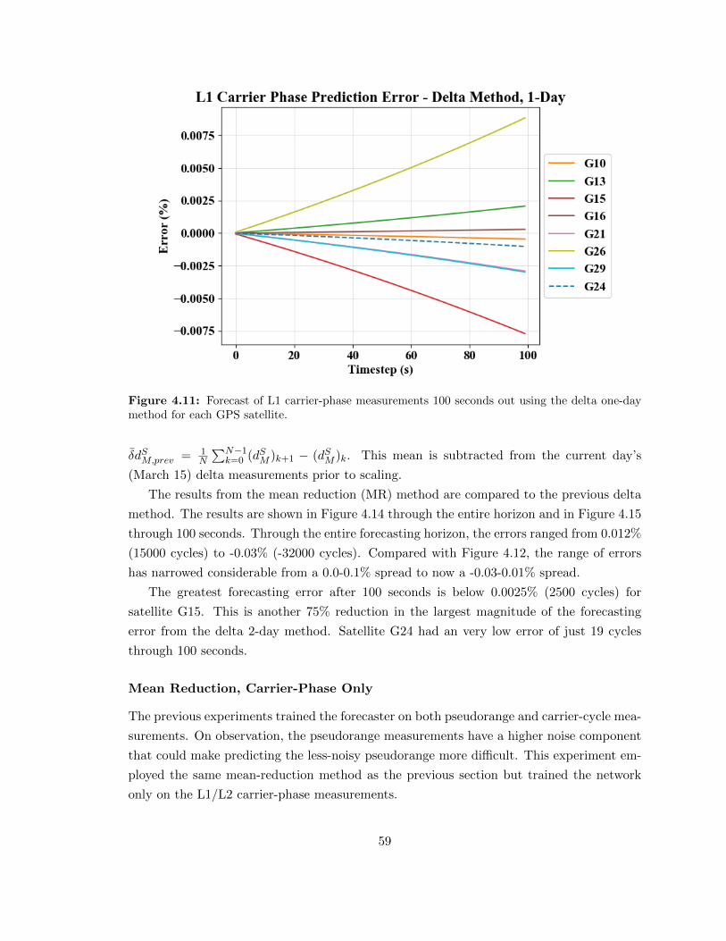
Figure 4.11: Forecast of L1 carrier-phase measurements 100 seconds out using the delta one-daymethod for each GPS satellite.

δdSM,prev = 1N

∑N−1k=0 (dSM )k+1 − (dSM )k. This mean is subtracted from the current day’s

(March 15) delta measurements prior to scaling.

The results from the mean reduction (MR) method are compared to the previous delta

method. The results are shown in Figure 4.14 through the entire horizon and in Figure 4.15

through 100 seconds. Through the entire forecasting horizon, the errors ranged from 0.012%

(15000 cycles) to -0.03% (-32000 cycles). Compared with Figure 4.12, the range of errors

has narrowed considerable from a 0.0-0.1% spread to now a -0.03-0.01% spread.

The greatest forecasting error after 100 seconds is below 0.0025% (2500 cycles) for

satellite G15. This is another 75% reduction in the largest magnitude of the forecasting

error from the delta 2-day method. Satellite G24 had an very low error of just 19 cycles

through 100 seconds.

Mean Reduction, Carrier-Phase Only

The previous experiments trained the forecaster on both pseudorange and carrier-cycle mea-

surements. On observation, the pseudorange measurements have a higher noise component

that could make predicting the less-noisy pseudorange more difficult. This experiment em-

ployed the same mean-reduction method as the previous section but trained the network

only on the L1/L2 carrier-phase measurements.

59

Figure 4.12: Forecast of L1 carrier-phase measurements 600 seconds out using the delta two-daymethod for each GPS satellite.

The L1 carrier-phase forecasting results for the MR-CO method are displayed in Fig-

ure 4.16 and Figure 4.17. Considering the entire forecasting horizon, the range of the errors

increased from the MR method to 0.01% to -0.08%. Through 100 seconds, the largest error

is -0.0020% (-2300 carrier cycles) for satellite G13. The lowest error is around -0.0001%

(less than 100 carrier cycles) for satellite G24.

Using only the carrier-phase measurements improved the forecasts for some measure-

ments. Satellite G15’s L1 carrier phase prediction error was kept under 0.0010% using

only the carrier cycles measurement, while the magnitude of G13’s prediction error in-

creased from 0.0010% to -0.0020%. Some vehicles have better predictions when training

the network with pseudorange and carrier-phase measurements, while others have worse

predictions.

60

Figure 4.13: Forecast of L1 carrier-phase measurements 100 seconds out using the delta two-daymethod for each GPS satellite.

Figure 4.14: Forecast of L1 carrier-phase measurements 600 seconds out using the delta mean-reduction method for each GPS satellite.

61

Figure 4.15: Forecast of L1 carrier-phase measurements 100 seconds out using the delta mean-reduction method for each GPS satellite.

Figure 4.16: Forecast of L1 carrier-phase measurements 600 seconds out using the delta mean-reduction, carrier-phase only method for each GPS satellite.

62

Figure 4.17: Forecast of L1 carrier-phase measurements 100 seconds out using the delta mean-reduction, carrier-phase only method for each GPS satellite.

63

4.6 Assessing RNN Measurement Predictions

The forecaster presented here was capable of making carrier-phase predictions with very

small percentile errors. Results for each forecaster type are summarized in Table 4.3 How-

ever, these very small percentile errors still translate to large errors in the carrier cycle

forecasts. The initial strategy of using the direct measurement data structure produced

the largest errors on the order of 5% relative to the true measurements. Using a the pre-

vious day’s measurements in addition to the target day’s measurements for training the

forecaster did not reduce the overall error using the direct method. In an attempt to reduce

the magnitude of numbers being predicted, the delta measurement method was employed

with successful results. Using a single day’s worth of measurements, the maximum error of

the forecaster using the delta method was less than 0.13%, a huge reduction compared to

the direct method. Using the previous day’s data reduced the maximum error to 0.11%.

The best forecasts were made using the delta measurement method, so other strategies

were explored to drive down the forecasting error. The mean-reduction (MR) method used

the mean delta measurement of the prior day’s dataset to further reduce the scale of the

target day’s dataset. This method had a dramatic effect in reducing the maximum error to

0.03%, a 73% reduction compared to the two-day delta forecaster. Next, the MR carrier-

cycles only method was employed. Disregarding the pseudorange measurements to train

the forecaster resulted in a larger error magnitude at the 600 second horizon. Some satellite

vehicles errors decreased, while others increased. The MR-CO method is considered a wash,

and the MR method was the most effective method used out of all the experiments.

Recall the general model for the carrier cycles measurement:

Φnu = λ−1[rnu + IΦ + TΦ] +

c

λ(δtu − δtn) +N + εnΦ,u (4.15)

the integer number of wavelength cycles N is an unobservable, to-be-determined quantity.

Errors in the carrier phase prediction for each satellite will cause the calculated N to diverge.

Table 4.3: Prediction error for each experiment at different forecasting horizons.

Forecaster Max Error100s (%) Max Error600s (%)

Direct, One-Day -1 -3Direct, Two-Day -1.5 -5Delta, One-Day 0.008 0.13Delta, Two-Day -0.008 -0.11Delta, Mean-Reduction 0.0022 -0.03Delta, Carrier-Only -0.0020 -0.08

64

4.6.1 Calculating the Position Solution

In each of the experiments, a RINEX file was created that replaced the true reference station

measurements with the forecasted measurements. The open-source software RTKlib was

used to post-process the faux user receiver measurements and forecasted measurements

to create a non-real-time RTK navigation solution [56]. Only one forecaster, the delta

mean-reduction forecaster, produced sufficient measurement predictions to create an RTK

navigation solution. After all, the end-goal is to produce a usable navigation solution.

Figure 4.18 shows the error between the solution using the true measurements and the

solution using the forecasted measurements. The RTK solution was only in floating-point

mode and never fixed-integer mode. The forecasting begins at 09:48:00. The North-South

and East-West position component errors diverge towards hundreds of meters quickly, while

the Up-Down component errors stay reasonable before diverging. Around the 09:50:45

mark, the solution reverts back to single-point position mode. While the RTK floating-

point position errors are absurdly large, this was the first time RTKlib was able to create

an RTK navigation solution using the forecasted reference station measurements.

The Up-Down component of the position has much lower error than the North-South

or East-West components. Figure 4.19 shows the error up to one minute after forecasting

begins. The error of the Up-Down component is below 2 meters for the first 12 seconds

below 10 meters for the first minute. This is an order of magnitude smaller than the East-

West error and two orders of magnitude smaller than the North-South error. The relative

difference in component errors could shed light on where weaknesses lie in the forecaster.

A reason that position solutions cannot be computed with post-processing is because the

forecasted measurement errors diverge relative to one another (not just absolutely). Recall

from Chapter 2, the concept of single-difference and double-difference measurements. When

performing differential carrier-phase navigation, the measurement itself is not as important

as the final double-differenced values used to resolve the integer ambiguities.

In hindsight, perhaps the single-differenced measurements between satellite vehicles

would have been a more suitable choice for training the forecaster and is suggested as

an avenue for future research. This idea was primitively tested by inserting a constant off-

set in the RINEX measurements (-10000) to each of the measurements. Post-processing a

position solution using this perturbed data maintained an accurate floating point solution.

Questions remain as to the applied efficacy of this approach, and the specific result omitted

from this thesis.

There was concern that the order that the time series were fed into the forecaster biased

the forecaster to favor some satellites over others. For example, satellite G24 often had the

lowest error out of all the vehicles as seen in Figure 4.12 and Figure 4.16. Trials were run

that shuffled the input and the output data without major effects.

65

Figure 4.18: NED position errors w.r.t. the original solution up to falling out of RTK mode.

66

Figure 4.19: NED position errors w.r.t. the original solution up to one minute after forecastingbegins.

67

4.7 Future Work

The work presented here did not reach the goal of creating a forecaster that can maintain

an RTK navigation solution after the loss of external reference data. However, as a general

forecaster, the network presented here is capable of very-accurate forecasts with errors

much less than 0.1%. There are many considerations for future work towards creating an

RNN-based forecaster to augment RTK operation.

Many parts of the work described here offer opportunities for future exploration and

iteration. While the final forecaster strategy presented was not able to reproduce usable

RTK solutions, each trial took a step forward in reducing the magnitude of the forecast-

ing error. Though the errors are too large for producing RTK solutions, perhaps such a

forecaster could be used for long-term, high-fidelity differential GPS positioning that uses

pseudorange corrections (PRC) that have a much lower magnitude than the measurements

discussed here.

A single RNN forecaster was used for all of the measurements from all of the satellite

vehicles. No information was passed into the RNN as to which measurements came from

which satellite. The internal weights of the RNN encapsulated all of the satellite vehicles at

the same time meaning computational overhead was reduced, but possible useful information

may have been lost. It could be that idiosyncrasies between satellites are lost inside the

bulk of the network. Rather than using a single forecaster, an architecture that can handle

subsets of satellites could be more appropriate. This could take the form of using the

satellite number as a network input or creating individual forecasters for each vehicle as an

example. As it stands now, this forecaster is vehicle agnostic.

The experiments carried out here used only a sliver of data (two hours from two days)

compared to the amount available. Many CORS networks, including MnCORS, have an

archive of measurements available as RINEX files for dozens of reference stations. There

could be opportunity into leveraging a large amount of GNSS measurement data to improve

the performance of an RNN forecaster. This would increase the likelihood that the forecaster

has seen some data trend in the past.

There are aspects of neural network design and implementation that were overlooked

and not discussed in this thesis. These include dropout and noise layers, more sophisticated

network topologies, and online training methods. This work is an initial step on developing

an RNN forecaster that can predict future time-series measurements with very little error.

As the state of the art of neural networks and deep learning is constantly changing, there

is much more to explore especially in the realm of time-series forecasting.

68

5. Conclusion

This thesis presented a technical background of global positioning satellite systems (GNSS)

and the real-time kinematic (RTK) positioning method of calculating precise position so-

lutions. It covered the basics of GNSS signals, the pseudorange and carrier phase, and

RTK navigation using these observables. Also introduced are common data formats used

for transferring GNSS-related information.

The growing availability of low-cost RTK receivers prompted an assessment of sev-

eral receivers using the Minnesota Continuously Operating Reference Station (MnCORS)

network. This assessment was performed for the Minnesota Department of Transporta-

tion (MnDOT). The study showed that the multifrequency Swift Piksi Multi had the best

accuracy and availability of the low-cost receivers while using a multifrequency antenna.

However, it demonstrated degraded metrics using the patch antenna and when operating in

non-ideal environments. The single-frequency low-cost receivers performed best in the rural

environment during static testing, but metrics degraded in other environments and during

the dynamic tests. The u-blox NEO-M8P and Emlid reach had the highest availability,

continuity and accuracy of the single-frequency low-cost receivers. The mid-range Hemi-

sphere Eclipse P307 outperformed all of the low-cost receivers during static and dynamic

testing in all environments. The performance of the Eclipse P307 came at a cost of around

$2000 versus $600 or less compared to the low-cost receivers. Low-cost receiver technology

is advancing, and some manufacturers including Swift and u-blox have released firmware

updates that may increase the capabilities of the receivers. Future work could investigate

the changes that these updates have had and investigating new hardware as it is released.

RTK navigation depends on a steady stream of GNSS data from a reference station, and

the position solution can be lost if the connection between the reference and primary receiver

is compromised In the final chapter, a recurrent neural-network (RNN) time-series forecaster

was prototyped to predict measurements for RTK operation. An RNN forecaster was trained

offline using measurement from MnCORS base stations, and it was found that using the

difference between subsequent measurements will result in an overall lower prediction error.

However, the prediction errors were too large to be useful for RTK positioning, though there

is likely room for improvement in the forecaster. Future work could include building upon

the current capabilities of RNN time series forecasting to increase the robustness of RTK

GNSS or investigating alternative approaches to this problem.

69

Bibliography

[1] Nathan F. Putman. “Inherited magnetic maps in salmon and the role of geomag-

netic change”. In: Integrative and Comparative Biology 55.3 (2015), pp. 396–405. issn:

15577023. doi: 10.1093/icb/icv020.

[2] Marie Dacke et al. “Dung beetles use the milky way for orientation”. In: Current

Biology 23.4 (2013), pp. 298–300. issn: 09609822. doi: 10.1016/j.cub.2012.12.034.

arXiv: 9809069v1 [arXiv:gr-qc].

[3] C. Evangelista et al. “Honeybee navigation: critically examining the role of the po-

larization compass”. In: Philosophical Transactions of the Royal Society B: Biological

Sciences 369.1636 (2014), pp. 20130037–20130037. issn: 0962-8436. doi: 10.1098/

rstb.2013.0037.

[4] Mai Thuy. Global Positioning System History. 2012. url: https://www.nasa.gov/

directorates/heo/scan/communications/policy/GPS{\_}History.html.

[5] United Nations Office for Outer Space Affairs. “Current and Planned Global and

Regional Navigation Satellite Systems and Satellite-based Augmentations Systems”.

In: (2010), p. 70. url: http://www.unoosa.org/pdf/publications/icg{\_}ebook.

pdf.

[6] Frank van Diggelen. “The Smartphone Revolution”. In: GPS World (Dec. 2009). url:

http://gpsworld.com/wirelesssmartphone-revolution-9183/.

[7] Alec Gorjestani et al. Part of the Intelligent Vehicle Initiative Driver Assistive Systems

for Snowplows. Tech. rep. University of Minnesota, 2003.

[8] XM395 Precision Mortar. 2015. url: https://www.orbitalatk.com/defense-

systems/.

[9] GPS.gov. Applications - Timing. 2014. url: https://www.gps.gov/applications/

timing/ (visited on 12/28/2017).

[10] Jessica Arlas and Sara Spangelo. “GPS Results for the Radio Aurora Explorer II

CubeSat Mission”. In: AIAA Region III Student Conference (2012), pp. 1–8. doi:

10.2514/6.2013-123.

[11] Pratap Misra and Per Enge. Global Positioning System - Signals, Measurements, and

Performance. Revised Se. Lincoln, Massachusetts: Ganga-Jamuna Press, 2011. isbn:

978-0-9709544-1-1.

[12] Charles C. Counselman et al. “Centimeter-Level Relative Positioning With GPS”. In:

Journal of Surveying Engineering 109.2 (1983), pp. 81–89.

70

[13] Bradford W. Parkinson and Stephen T. Powers. “Part 2: The Origins of GPS, Fighting

to Survive”. In: GPS World (June 2010). url: http://gpsworld.com/origins-gps-

part-2-fighting-survive/.

[14] Chris Rizos. “Alternatives to current GPS-RTK services and some implications for

CORS infrastructure and operations”. In: (2007). doi: 10.1007/s10291-007-0056-x.

[15] “Last Block IIF to replace oldest GPS satellite”. In: GPS World (Jan. 2016). url:

http://gpsworld.com/last-block-iif-to-replace-oldest-gps-satellite/.

[16] Col. Steven Whitney. “Directions 2018: The GPS year in review”. In: GPS World

(Dec. 2017). url: http://gpsworld.com/directions-2018-the-gps-year-in-

review/.

[17] US Department Of Defense. “Global Positioning System Standard Positioning Ser-

vice”. In: gps.gov September (2008), pp. 1 –160. url: http : / / www . gps . gov /

technical/ps/2008-SPS-performance-standard.pdf.

[18] NIMA. “Department of Defense World Geodetic System 1984”. In: Technical Report

8350.2, Third Edition (2000), p. 175. doi: TR8350.2. url: http://earth-info.nga.

mil/GandG/publications/tr8350.2/wgs84fin.pdf.

[19] Martina Szabova and M Sc. “Survey Of GNSS Coordinates Systems”. In: 12.24 (2016),

pp. 33–42. doi: 10.19044/esj.2016.v12n24p33.

[20] navy.mil. USNO GPS Time Transfer. url: tycho.usno.navy.mil/gpstt.html.

[21] P. J. G. Teunissen, P. J. de Jonge, and Christian C. C. J. M. Tiberius. “The LAMBDA-

Method for Fast GPS Surveying”. In: Proceedings of International Symposium �GPS

technology applications� 1 (1995), pp. 203–210.

[22] International GNSS Service ( IGS ). “The Receiver Independent Exchange Format”.

In: IGS Workshop 2012 104 (2012), pp. 1–74.

[23] RTCM SPECIAL COMMITTEE NO. 104. RTCM STANDARD 10403.2 DIFFER-

ENTIAL GNSS (GLOBAL. Tech. rep. Arlington, VA: Radio Technical Commission

for Maritime Services.

[24] NMEA 0183 Interface Standard. Standard. Severna Park, MD: National Marine Elec-

tronics Association, Nov. 2008.

[25] Li Ta Hsu et al. “Multiple Faulty GNSS Measurement Exclusion Based on Consistency

Check in Urban Canyons”. In: IEEE Sensors Journal 17.6 (2017), pp. 1909–1917. issn:

1530437X. doi: 10.1109/JSEN.2017.2654359.

71

[26] Trevor Layh et al. “A recovery system for SUAV operations in GPS-denied environ-

ments using timing advance measurements”. English (US). In: Institute of Navigation

International Technical Meeting 2015, ITM 2015. United States: Institute of Naviga-

tion, Jan. 2015, pp. 293–303.

[27] Laurie Bedord. “John Deere Ramps Up RTK Coverage”. In: Successful Farming (Apr.

2016). url: https://www.agriculture.com/content/john-deere-ramps-up-rtk-

coverage.

[28] RTCM SPECIAL COMMITTEE NO. 104. RTCM STANDARD 10410.0. Tech. rep.

Arlington: Radio Technical Commission for Maritime Services, 2001.

[29] MnDOT. MnCORS GNSS Network. 2018. url: http://www.dot.state.mn.us/

surveying/cors/.

[30] Yijian Cui et al. “Feasibility analysis of low-cost GNSS receivers for achieving re-

quired positioning performance in CAV applications”. In: 2017 Forum on Cooperative

Positioning and Service, CPGPS 2017 (2017), pp. 355–361. doi: 10.1109/CPGPS.

2017.8075154.

[31] Antennas. NOT-20140609a. Navcom. 2014.

[32] ANN-MS, Active GPS antenna. UBX-15025046. R14. u-blox. Nov. 2017.

[33] Hamid Mokhtarzadeh, Adhika Lie. NavPy. Version 1.0. url: https://github.com/

NavPy/NavPy.

[34] Knio. Pynmea2. Version 1.12.0. url: https://github.com/Knio/pynmea2.

[35] Gary Chisholm. “Virtual reference station improved efficiency”. In: International

Ocean Systems 6.6 (2002), pp. 10–12. issn: 14604892. doi: 10.5081/jgps.1.2.137.

[36] J. Jackson. PyRTK Utility. 2017. url: https://github.umn.edu/IVLab/gnss-

eval/tree/master/Utility.

[37] MnDOT. Interactive Geodetic Monument Viewer. 2018. url: https://www.dot.

state.mn.us/maps/geodetic/.

[38] SF-3050. NCT-20140609a. Navcom. 2014.

[39] James E. Gentle. “Mathematical and Statistical Preliminaries”. In: Computational

Statistics. New York, NY: Springer New York, 2009, pp. 5–79. isbn: 978-0-387-98144-

4.

[40] Michael S. Braasch (Ohio University). “Multipath Effects”. In: Global Positioning

System: Theory and Applications. Ed. by Bradford W. Parkinson and James J. Spilker

Jr. AIAA, 1995, pp. 547–568.

72

[41] u-blox announces u-blox F9 robust and versatile high precision positioning technology

for industrial and automotive applications. Thalwil, Switzerland, 2018. url: https:

//www.u-blox.com/en/press-releases/u-blox-announces-u-blox-f9-robust-

and-versatile-high-precision-positioning-technology.

[42] Tomoji Takasu and Akio Yasuda. “Evaluation of RTK-GPS performance with low-

cost single-frequency GPS receivers”. In: Proceedings of international symposium on

GPS/GNSS (2008), pp. 852–861.

[43] “Dual Frequency, Carrier Phase Differential GPS Augmentation”. In: Intelligent Trans-

portation Systems (), p. 43.

[44] Alex Graves. “Generating Sequences With Recurrent Neural Networks”. In: (2013),

pp. 1–43. issn: 18792782. doi: 10.1145/2661829.2661935. arXiv: 1308.0850.

[45] Daniel Zoran et al. “Playing Atari with Deep Reinforcement Learning”. In: arXiv

32.Ijcai (2016), pp. 1–9. issn: 10495258. doi: 10.1038/nature14236. eprint: 1507.

01526.

[46] Yanrui Geng. “Online DGPS correction prediction using recurrent neural networks

with unscented Kalman filter”. In: International Global Navigation Satellite Systems

Society IGNSS Symposium, The University of New South Wales, Sydney, Australia

(2007), pp. 4–6.

[47] Arif Indriyatmoko et al. “Artificial neural networks for predicting DGPS carrier

phase and pseudorange correction”. In: GPS Solutions 12.4 (2008), pp. 237–247. issn:

10805370. doi: 10.1007/s10291-008-0088-x.

[48] Sohel Ahmed, Quddusa Sultana, and K. Deergha Rao. “Comparative analysis of

DGPS predicted corrections using dynamic neural networks”. In: 2014 IEEE Interna-

tional Conference on Vehicular Electronics and Safety, ICVES 2014 m (2015), pp. 61–

65. doi: 10.1109/ICVES.2014.7063725.

[49] Warren S. McCulloch and Walter Pitts. “A logical calculus of the ideas immanent in

nervous activity”. In: The Bulletin of Mathematical Biophysics 5.4 (1943), pp. 115–

133. issn: 00074985. doi: 10.1007/BF02478259. arXiv: arXiv:1011.1669v3.

[50] Czxttkl. Convolutional Neural Network Simple Tutorial. url: https://nb4799.neu.

edu/wordpress/?p=246 (visited on 05/11/2018).

[51] Sepp Hochreiter and Jurgen Jurgen Schmidhuber. “LSTM”. In: Neural Computation

9.8 (1997), pp. 1–32. issn: 0899-7667. doi: 10.1162/neco.1997.9.8.1735. arXiv:

1206.2944.

[52] J. Jackson. RTKnet. 2018. url: https://github.umn.edu/jacks974/RTKnet.

73

[53] MnDOT. MnCORS FTB Website. 2018. url: ftp://ftp.olmweb.dot.state.mn.

us/.

[54] Francois Chollet et al. Keras. https://github.com/keras-team/keras. 2015.

[55] Diederik P. Kingma and Jimmy Ba. “Adam: A Method for Stochastic Optimization”.

In: (2014), pp. 1–15. doi: http://doi.acm.org.ezproxy.lib.ucf.edu/10.1145/

1830483.1830503. arXiv: arXiv:1412.6980v9.

[56] Tomoji Takasu et al. RTKlib. https://github.com/tomojitakasu/RTKLIB/tree/

rtklib_2.4.3. 2017.

74

A. Appendix

Figure A.1: Location of the TURKEY MN037 marker used for static testing.

75

Figure A.2: Location of the UNIVERSITY1934 marker used for static testing.

76

Figure A.3: Location of the SCHREIBER marker used for static testing.

77

Figure A.4: The bridges route for dynamic data collection.

78

Figure A.5: The urban route for dynamic data collection.

79

Figure A.6: Absolute prediction error for the direct 1-day method.

Figure A.7: Absolute prediction error for the direct 2-day method.

80

Figure A.8: Absolute prediction error for the delta 1-day method.

Figure A.9: Absolute prediction error for the delta 2-day method.

81

Figure A.10: Absolute prediction error for the delta mean-reduction method.

Figure A.11: Absolute prediction error for the delta mean-reduction, carrier-only method.

82

Real-time Kinematic Positioning: Background, Assessment ...

Documents

Transcript of Real-time Kinematic Positioning: Background, Assessment ...