Real-time Forecasts of Tomorrow’s Earthquakes in

California: a New Mapping Tool

By Matt Gerstenberger1, Stefan Wiemer2 and Lucy Jones1

Open-File Report 2004-1390

2004

Any use of trade, firm, or product names is for descriptive purposes only and does not imply

endorsement by the U.S. Government.

U.S. DEPARMENT OF THE INTERIOR

U.S. GEOLOGICAL SURVEY

1U.S. Geological Survey, 525 S. Wilson Ave. Pasadena, CA, 91106, USA

2Swiss Seismological Service ETH-Hoenggerberg/HPP-P7 CH-8093 Zurich, Switzerland

1

Abstract

We have derived a multi-model approach to calculate time-dependent earthquake hazard resulting

from earthquake clustering. This open-file report explains the theoretical background behind the

approach, the specific details that are used in applying the method to California, as well as the

statistical testing to validate the technique. We have implemented our algorithm as a real-time tool

that has been automatically generating short-term hazard maps for California since May of 2002,

at http://step.wr.usgs.gov

1 Introduction

Earthquake clustering, particularly in relationship to aftershocks, is an emperically defined, al-

beit not perfectly understood seismic phenomena. We have developed a real-time tool that com-

bines and expands on previous research in earthquake clustering with current estimates of long-

term hazard to create probabilistic forecasts. We combine an existing time-independent hazard

model based on geological data and historical earthquakes with models describing time-dependent

earthquake clustering. The result is a map giving the probability of strong shaking at any loca-

tion in California within the next 24-hours, updated within minutes and available on the web at

http://step.wr.usgs.gov. This report is a guide to understanding how this code works and how we

have validated the results.

We expect the tool to foster increased awareness of seismic hazard in the general public, im-

proved emergency response, and increased scientific understanding of short term seismic hazard.

In the real time format, the maps provide:

• Assistance in immediate decisions by emergency planners and scientists related to the oc-

currence of a damaging earthquake after a large mainshock

• Information for city managers, etc., to assist in decisions about shutting down certain ser-

vices and entering damaged buildings after a large mainshock.

• A continually updated source of information that is easily available to the general public and

media.

Scientific advancements are in four main areas:

• Development of a real time probabilistic analysis tool

2

• Increased understanding of spatial variability in aftershock sequences

• Implementation of a methodology for automating decisions related to model comparisons

• Establishment of a null hypothesis in time dependent and conditional probabilistic seismic

hazard analysis.

Validation of a forecast model is a necessary part of its development. While other models have

been developed to characterize short-term hazard [Kagan and Jackson, 2000], currently there is

no established null hypothesis against which to test other models. By formulating our model as

we have, we believe we have created an appropriate null hypothesis for testing other conditional

probabilistic hazard and short-term seismicity related ideas (i.e. static and dynamic stress changes

[Harris, 1998; Stein et al., 1992] accelerated moment release, [Bufe and Varnes, 1996] and quies-

cence before large aftershocks [Matsu’ura, 1986; Ogata, 1992]. We hope that the provision of this

null hypothesis will encourage the development of other short-term models and also the participa-

tion of these models in model validation through statistical testing. This initiative is already well

underway for southern California with the Regional Earthquake Likelihood Modeling (RELM)

group of the Southern California Earthquake Center (http://www.relm.org). Much of our model

has been developed with the goals of RELM in mind.

2 Background

The fundamental concept we used is an earthquake hazard map. These maps display the proba-

bility of exceeding a level of ground shaking in a specified time period, drawn from a model of

earthquake occurrence and an estimate of the distribution of shaking that will result from each

earthquake. Long term, probabilistic seismic hazard analysis (PSHA) and maps have been in use

for a number of decades [Cornell, 1968; Frankel et al., 1996; Giardini, 1999] and are widely used

in applications such as long term hazard mitigation through the design of appropriate building

codes and the selection of relatively safe locations for building nuclear facilities. The maps display

probabilities of exceeding a specified level of ground shaking over a long time period, typically on

the order of 50 years.

We have expanded the concept of a hazard map by incorporating information about short-

term earthquake clustering. A simple schematic of how probabilities due to both foreshocks and

aftershocks develop is illustrated in figure 1. Reasenberg and Jones [1989, 1990 & 1994] developed

a simple earthquake clustering model, based on the modified Omori law and the Gutenberg-Richter

relationship, to describe this increase in probability of future events following any other event for

time periods ranging from days to weeks. However, the model deals with time and magnitude only,

not space.

3

Foreshock:

no subsequent

mainshock

Foresock with subsequent

mainshock and aftershock

sequence

Time

Ma

gP

rob

ab

ilit

y

background

Figure 1: Schematic view of aftershocks and potential foreshocks and their effect on time-dependent probabilities of future ground shaking.Bottom Axis: earthquakes of varying sizesincluding an aftershock sequence.Top axis: probabilistic hazard forecast from a simple clusteringmodel based on the occurrence of each earthquake.

Reasenberg & Jones (R&J) made three assumptions about the distribution of aftershocks. First,

they assumed that the aftershock magnitudes follow a Gutenberg-Richter relationship [Gutenberg

and Richter, 1954], so that the number of aftershocks (N) is proportional to the aftershock magni-

tude,M, as:

N ∝ 10bM (1)

whereb parameterizes the ratio of small events to large events. Second, they assumed the rate

of aftershocks varies with time as in the modified Omori Law [Utsu, 1995], so that the rate of

aftershocks depends on the time since the mainshock,t, as:

N ∝ (t +c)−p (2)

wherec and p are empirically determined constants. Third, they assumed that the variation in

aftershock rate with the mainshock magnitude, Mm, could be expressed through the Gutenberg-

Richter relation, and thus:

N ∝ 10bMm

These three assumption were combined to give the rate of aftershocksλ(t,Mc) larger than a mag-

nitude threshold,Mc and occurring at time t:

4

λ(t,M) =10a′+b(Mm−M)

(t +c)p (3)

M ≥Mc

From this rate, and assuming a non-homogeneous Poissonian occurrence of aftershocks, the proba-

bility of events occurring above a given magnitude and within a given time period can be calculated

as follows:

P = 1−exp

[Zλ(t,Mc)δt

](4)

Thus the rate of aftershocks and therefore the probability of future aftershocks can be expressed

with four parameters,a′, b, c, andp. Reasenberg and Jones applied this model to California and

determined these parameters for all sequences with mainshock magnitudeM ≥ 5.0 from 1932

to 1987. The generic aftershock sequence parameters have been defined as the mean of the ap-

proximately normal distributions of the constants from that dataset (a′g = -1.67,bg = .91,cg=.05,

pg=1.08).

Figure 2 shows how forecasted rates of aftershocks from the generic model compare to ob-

served rates from 1988-2002. This is an independent test which shows that the generic model

is a reasonable first-order approximation of aftershock sequences occurring in the last 15 years.

While the rates from the generic values do give a reasonable first estimate of aftershock hazard,

they do not allow for variations in individual sequences by including any information specific to

an individual aftershock sequence other than the mainshock size. As the sequences progresses,

to best combine the information from the generic estimates and the sequence specific estimates,

Reasenberg & Jones proposed a technique based on Bayesian estimation.

3 A Real-Time Model

The method we describe in this report is an expansion of the Reasenberg and Jones model into a

fully automated real time short term PSHA mapping tool. The maps combine information from

long term hazard with short term hazard based on Reasenberg and Jones to produce a map showing

the probability of exceeding a peak ground acceleration (PGA) level of .126 within a given time

period, which is typically 24 hours.

We have expanded Reasenberg and Jones in several ways:

• The spatial distribution of the increased earthquake occurrence is computed: both the dis-

tribution of the overall hazard of the sequence around the mainshock fault, and the spatial

variability within the sequence.

5

Figure 2: Calculated and observed rates of events≥M4 in 24-hour-long intervals following main-shocks occurring between 1988 and 2002 in southern California. Dashed lines show the ratesforecasted by the generic California clustering model for the mainshock magnitude (M) shown.Correspondingly, solid lines show the observed rates ofM ≥ 4.0 aftershocks for same time peri-ods following mainshocks with magnitudeM±0.5. The aftershock zones are defined as the areaswithin one rupture length of the main shock epicenter.

• The combined hazard from multiple aftershock sequences and cascading sequences is in-

cluded.

• A hazard assessment of seismic shaking from all possible magnitudes is calculated.

• The hazard is computed automatically for real-time use.

Our final forecast model is derived from several “model elements.” These model elements, which

we will define later, are earthquake rate forecasting techniques based on the previously mentioned

seismicity parameters. Using the analogy of the logic tree approach often used in standard PSHA,

our final forecast may be based on contributions from more than one model element at any given

time. However, because of the need for real-time processing, the combining of the model ele-

ments must be based on an automated decision. Using the corrected Akaike Information Criterion

(AICc) [Burnham and Anderson, 2002] we compare all model elements and derive a weighted and

combined forecast of the future rate of events.

6

This section gives a detailed description of the above process starting from recording the oc-

currence of a new event to the creation of a hazard map. In the following section, a detailed flow

chart is presented.

3.1 The Data

The model is applied to the entire state of California. We collect information on earthquakes up

to 0.5-degrees beyond the state boundaries. As implemented, maps are created for the whole state

and, to provide more detail, for individual 3-degree squares across the region. Rate forecasts are

calculated on a 0.05-degree grid.

Real-time earthquake hypocenters and magnitudes are obtained from the California Integrated

Seismic Network via QDDS, a U.S. Geological Survey application for distributing and receiv-

ing events in real time (ftp://clover.wr.usgs.gov/pub/QDDS/QDDS.html ). As QDDS is a

real-time application and collects earthquake data from a number of sources, duplicate earthquake

locations and magnitudes can be received. Additionally, updated locations or magnitudes are some-

times distributed after the initial data have been received. Provisions have been made in the code

to remove duplicate events and to include updated information relevant to a particular event. The

initial locations from QDDS are computed automativally and can contain errors. The smoothing

implicit in the gridding algorithm we describe below negates much of the effects of location errors,

but it also limits the resolution of spatially variability that we are able to achieve.

3.2 Spatial Definition of the Aftershock Zone

For every recorded event, we must determine if the event should be modeled as an aftershock to

some previous mainshock. The model defines aftershocks based only on space and time; therefore

we must assign an aftershock zone toeveryevent. Additionally, each time the code is executed,

an aftershock zone is estimated or re-estimated for each event. Any single event is only allowed to

be the aftershock to one mainshock. If the event falls within the spatial and temporal definition of

the aftershock zones for more than one mainshock, the event will be assigned only to the largest

mainshock.

Three types of aftershock zones are defined based on increasing complexity and amount of data

required. Here we discuss the spatial component of the aftershock zone; the temporal component

is explained in the 3.8.1.

• AftershockZone Type I: The least complex zone is based on a rupture length from the

Wells and Coppersmith relationship for subsurface rupture [Wells and Coppersmith, 1994]:

7

log(RLD) = −2.44+ .58∗M whereRLD is the subsurface rupture length andM is the mo-

ment magnitude. The zone is defined as the region within one rupture length of the epicenter

of the event, resulting in a circular aftershock zone. This method requires only the event

magnitude and location.

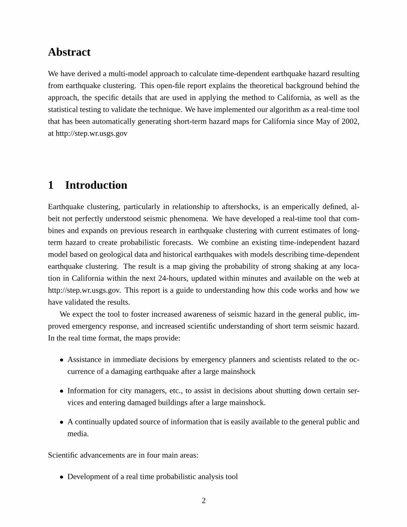
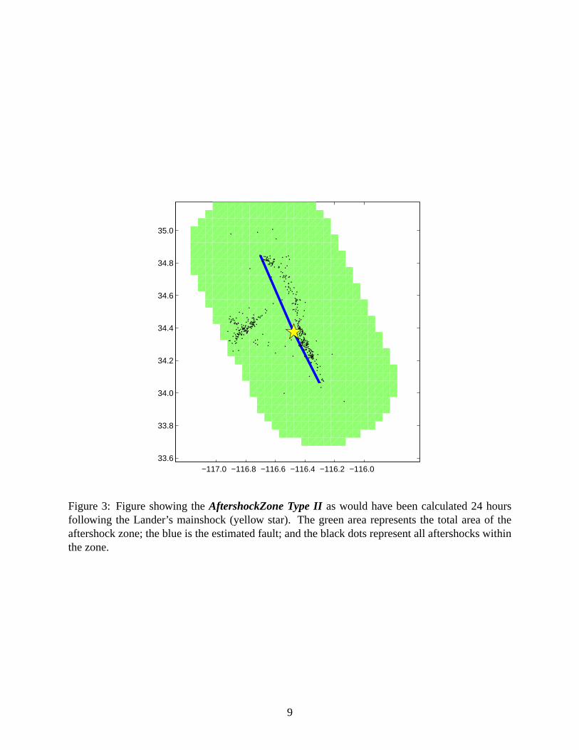
• AftershockZone Type II: When at least 100 aftershocks have been recorded within anAf-

tershockZone Type I, we use these events to define the aftershock zone based on the spatial

distribution of the aftershocks themselves. We estimate the fault location in three steps:

1. Find the individual most northern, southern, eastern and western events (4 total events).

Ignore the most extreme 1% events in all cases (e.g. ignore the 1% most northern

events).

2. Using these four events, select the longest of the east-west or north-south dimension

(length) and use the two events delineating this dimension to define the end-points of

the fault.

3. Use these end-points to create a two segment segment fault that passes through the

mainshock epicenter.

All events within one half of a fault length of the fault (as defined by Wells and Coppersmith)

are considered aftershocks. A future improvement toType IIzones will be to allow for a two-

dimensional fault representation for thrust faults. An example of a Type II zone as calculated

for Landers is shown in figure 3.

• AftershockZone Type III: Finally, if a fault rupture model has been calculated externally, we

manually input this model and override the automatically calculated aftershock zones. The

distance that the aftershock zone extends from the fault is part of the input model. Currently

this last model is only two dimensional and is is only available for the largest mainshocks

and could take a day or more after the mainshock before it is available. The reliance on

the use of the surface expression of the fault limits the usability of this type of zone (e.g., a

Type III zone was not applied to the Northridge earthquake because the surface fault will not

represent the actual aftershock zone) and is an example of future work needed for the model.

It should also be pointed out that the use of this externally input model isnot an automated

decision and requires input from an operator at the time of the fault model’s implementation.

An example of aType III zone using the Wald and Heaton [1994] slip model is shown

in the right panel of Figure 3. In this case the radius would be based on a seismologist’s

interpretation of the spatial extent of the seismicity.

8

−117.0 −116.8 −116.6 −116.4 −116.2 −116.033.6

33.8

34.0

34.2

34.4

34.6

34.8

35.0

Figure 3: Figure showing theAftershockZone Type IIas would have been calculated 24 hoursfollowing the Lander’s mainshock (yellow star). The green area represents the total area of theaftershock zone; the blue is the estimated fault; and the black dots represent all aftershocks withinthe zone.

9

r1r3

r2

Figure 4: Cartoon of 3 possible aftershock zone models for Landers.Left -Type I: Simple modelbased on 1 Wells & Coppersmith radius (r1) from mainshock epicenter.Center-Type II: Syntheticfault model keeping all events within 1/2 of a Wells & Coppersmith radius (r2).Right-Type III :External model based on the slip model of Wald and Heaton [1994] and keeping all events withingiven radius r3.

3.3 Parameter Estimation and Magnitude of Completeness

To determine the spatial definition of the aftershock zone for a given mainshock as described above,

we use all possible aftershocks regardless of magnitude. However, we must only use events larger

than the the magnitude threshold of completeness,Mcto estimate the parameters (a,b,c & p) for

the rate forecast.Mc is estimated using power law fitting techniques as described in [Wiemer and

Wyss, 2000]. In all cases, we estimateMc for the entire aftershock sequence. When calculating

spatially varying rates, we also estimateMc independently for the set of events for each grid node.

All events smaller thanMc are removed from the corresponding region. Both types ofMc are

re-estimated every time the code is initiated.

The parameters of an aftershock distribution are quite sensitive to the assumed magnitude of

completeness, and some catalogs appear not to be quite complete at the level implied by a formal

estimate ofMc. For this reason we take a somewhat conservative approach and assume the mag-

nitude of completeness to be 0.2 units larger than the formal estimate. Furthermore, recent studies

find that the magnitude of completeness is much larger immediately following an earthquake, be-

cause of the practical problem of identifying individual aftershocks when their records overlap.

For this reason we estimate the model parameters using only aftershocks more than 0.2 days after

the mainshock, provided that there are at least 100 such events. If not, we use all available events

in the sequence.

3.4 Spatial Distribution of the Aftershock Productivity

The productivity constant,a′ in Equation 3, defines the total rate of aftershocks for the whole

aftershock zone. In order to create a map, the aftershock rate must be distributed appropriately

10

Afte

rsh

ock

de

nsi

ty (

2-8

5 d

ays)

0 50 100

105

104

103

102

101

Distance from Mainshock Fault (km)

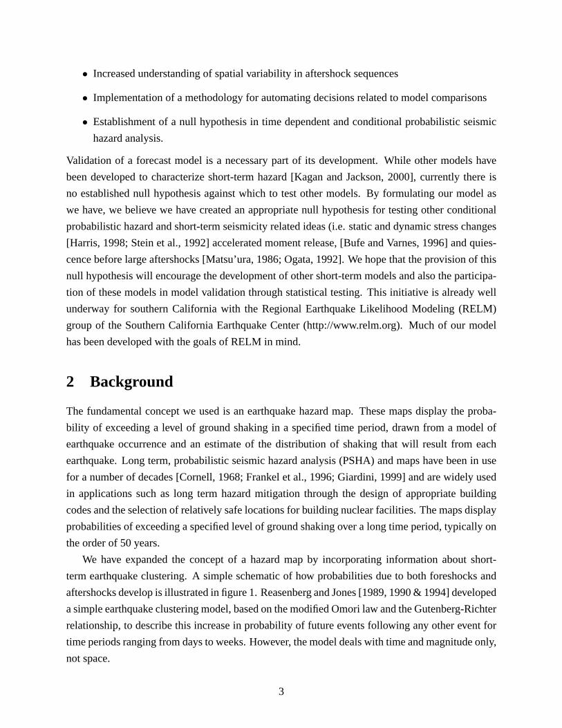
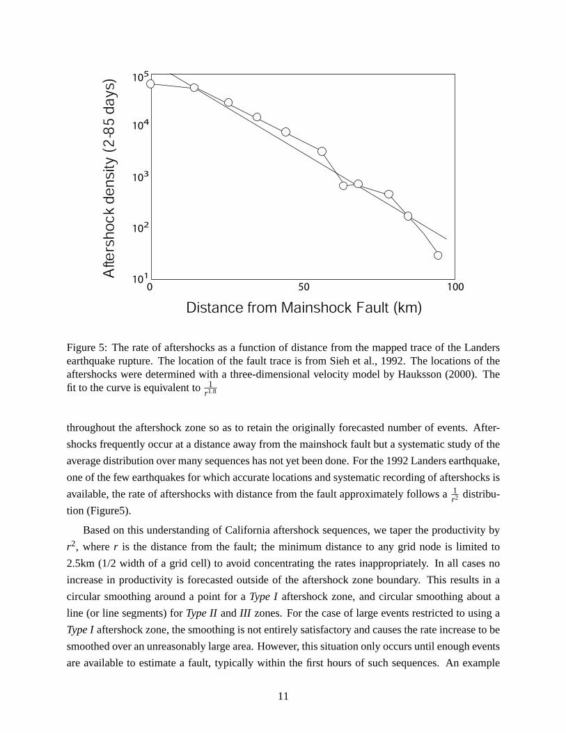
Figure 5: The rate of aftershocks as a function of distance from the mapped trace of the Landersearthquake rupture. The location of the fault trace is from Sieh et al., 1992. The locations of theaftershocks were determined with a three-dimensional velocity model by Hauksson (2000). Thefit to the curve is equivalent to1

r1.8

throughout the aftershock zone so as to retain the originally forecasted number of events. After-

shocks frequently occur at a distance away from the mainshock fault but a systematic study of the

average distribution over many sequences has not yet been done. For the 1992 Landers earthquake,

one of the few earthquakes for which accurate locations and systematic recording of aftershocks is

available, the rate of aftershocks with distance from the fault approximately follows a1r2 distribu-

tion (Figure5).

Based on this understanding of California aftershock sequences, we taper the productivity by

r2, wherer is the distance from the fault; the minimum distance to any grid node is limited to

2.5km (1/2 width of a grid cell) to avoid concentrating the rates inappropriately. In all cases no

increase in productivity is forecasted outside of the aftershock zone boundary. This results in a

circular smoothing around a point for aType I aftershock zone, and circular smoothing about a

line (or line segments) forType II andIII zones. For the case of large events restricted to using a

Type Iaftershock zone, the smoothing is not entirely satisfactory and causes the rate increase to be

smoothed over an unreasonably large area. However, this situation only occurs until enough events

are available to estimate a fault, typically within the first hours of such sequences. An example

11

0.001

116.0˚ W

34.0˚ N

35.0˚ N

0 50 100 km10 0 50 100 km10

.65.325

k value

Figure 6: Plot of the smoothedk value one day after the Landers mainshock; an external faultmodel has been input to define the aftershock zone. The aftershock zone width was defined usinga 60km half-width. The clear focusing of the rates along the fault is apparent in the figure.

of a smoothed aftershock rate (the 1992,Mw 7.3 Landers, California earthquake) is show in figure

6. The focusing of the rates in the 1 or 2 grid nodes (grid size: 5kmx5km) either side of the fault

is clear; the deepest red nodes correspond directly to the input fault model. Additionally, figure 7

shows the progression from aType I aftershock zone toType III for the Hector Mine aftershock

sequence.

3.5 Secondary Events

An inherent limitation of the modified Omori law is that it assumes the occurrence of an individual

aftershock has no effect on the rate of aftershock production of the overall sequence. Only the

mainshock is allowed to excite an aftershock sequence; individual aftershocks do not contribute

any rate changes of their own. In reality, secondary aftershock sequences are often observed

[Ogata, 1999] with large aftershocks causing an increase in the aftershock rate in their immedi-

ate vicinity. All aftershocks appear to impart some change to the regional stress field, and larger

aftershocks can cause a significant change in the rate of event production.

We account for these cascading aftershock sequences in our model by superimposing Omori

12

7 d

ays

afte

r

90 d

ays

afte

r1

min

ute

aft

er

1 d

ay a

fter

1 ye

ar a

fter

1 m

inu

te b

efo

re

0.003 .3 300

Forecasted number of events above background

Figure 7: Forecasted number of events (M > 4) above the background level for the Hector Mineaftershock sequence. Times are relative to the mainshock. The progression from a 100% genericmodel element using aType Iaftershock sequence 1 minute and 1 day after the event to a combi-nation of the three model elements is apparent 7 days after the event. The non-symmetric spatialvariability in the rates at day one is due to secondary sequences. For simulation, aType III (after-shock zone) fault based on Ji et.al. [2000] and an emperically determined radius is allowed oneday after the mainshock.

13

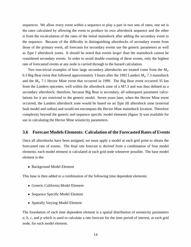
sequences. We allow every event within a sequence to play a part in two sets of rates; one set is

the rates calculated by allowing the event to produce its own aftershock sequence and the other

is from the recalculation of the rates of the initial mainshock after adding the secondary event to

the sequence. Because of the difficulty in distinguishing aftershocks of secondary events from

those of the primary event, all forecasts for secondary events use the generic parameters as well

asType I aftershock zones. It should be noted that eventslarger than the mainshock cannot be

considered secondary events. In order to avoid double counting of these events, only the highest

rate of forecasted events at any node is carried through to the hazard calculation.

Two non-trivial examples of how large secondary aftershocks are treated come from theMw

6.3 Big Bear event that followed approximately 3 hours after the 1992 LandersMw 7.3 mainshock

and theMw 7.1 Hector Mine event that occurred in 1999. The Big Bear event occurred 35 km

from the Landers epicenter, well within the aftershock zone of a M7.3 and was thus defined as a

secondary aftershock; therefore, because Big Bear is secondary, all subsequent parameter calcu-

lations for it are restricted to the generic model. Seven years later, when the Hector Mine event

occurred, the Landers aftershock zone would be based on anType III aftershock zone (external

fault model and radius) and would not encompass the Hector Mine mainshock location. Therefore

complexity beyond the generic and sequence specific model elements (figure 3) was available for

use in calculating the Hector Mine seismicity parameters.

3.6 Forecast Models Elements: Calculation of the Forecasted Rates of Events

Once all aftershocks have been assigned, we must apply a model at each grid point to obtain the

forecasted rate of events. The final rate forecast is derived from a combination of four model

elements; each model element is calculated at each grid node whenever possible. The base model

element is the:

• Background Model Element

This base is then added to a combination of the following time dependent elements:

• Generic California Model Element

• Sequence Specific Model Element

• Spatially Varying Model Element

The foundation of each time dependent element is a spatial distribution of seismicity parameters

a, b, c, andp which is used to calculate a rate forecast for the time period of interest, at each grid

node, for each model element.

14

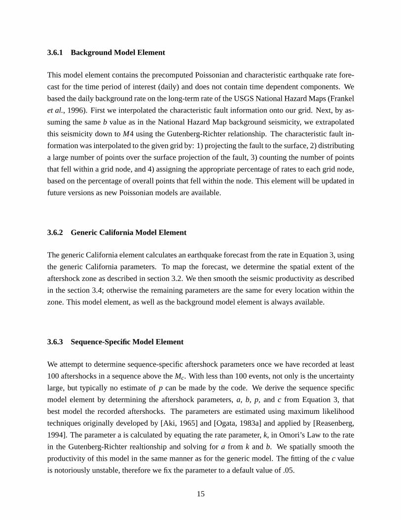
3.6.1 Background Model Element

This model element contains the precomputed Poissonian and characteristic earthquake rate fore-

cast for the time period of interest (daily) and does not contain time dependent components. We

based the daily background rate on the long-term rate of the USGS National Hazard Maps (Frankel

et al., 1996). First we interpolated the characteristic fault information onto our grid. Next, by as-

suming the sameb value as in the National Hazard Map background seismicity, we extrapolated

this seismicity down toM4 using the Gutenberg-Richter relationship. The characteristic fault in-

formation was interpolated to the given grid by: 1) projecting the fault to the surface, 2) distributing

a large number of points over the surface projection of the fault, 3) counting the number of points

that fell within a grid node, and 4) assigning the appropriate percentage of rates to each grid node,

based on the percentage of overall points that fell within the node. This element will be updated in

future versions as new Poissonian models are available.

3.6.2 Generic California Model Element

The generic California element calculates an earthquake forecast from the rate in Equation 3, using

the generic California parameters. To map the forecast, we determine the spatial extent of the

aftershock zone as described in section 3.2. We then smooth the seismic productivity as described

in the section 3.4; otherwise the remaining parameters are the same for every location within the

zone. This model element, as well as the background model element is always available.

3.6.3 Sequence-Specific Model Element

We attempt to determine sequence-specific aftershock parameters once we have recorded at least

100 aftershocks in a sequence above theMc. With less than 100 events, not only is the uncertainty

large, but typically no estimate ofp can be made by the code. We derive the sequence specific

model element by determining the aftershock parameters,a, b, p, andc from Equation 3, that

best model the recorded aftershocks. The parameters are estimated using maximum likelihood

techniques originally developed by [Aki, 1965] and [Ogata, 1983a] and applied by [Reasenberg,

1994]. The parameter a is calculated by equating the rate parameter,k, in Omori’s Law to the rate

in the Gutenberg-Richter realtionship and solving fora from k andb. We spatially smooth the

productivity of this model in the same manner as for the generic model. The fitting of thec value

is notoriously unstable, therefore we fix the parameter to a default value of .05.

15

Total number of events> Mc Radius≤ 1000 15km

> 1000& ≤ 1500 12km> 1500& ≤ 2000 10km

> 2000 7.5km

Table 1: The radius used for the seismicity parameter calculation, dependent on the number ofavailable events >Mc.

3.6.4 Spatially Varying Model Element

The final element, the spatially varying element, is based on spatial variations in the aftershock

parameters. When examining aftershock sequences, researchers have seen strong spatial variations

in seismicity parameters [Wiemer, 2002; Wiemer and Katsumata, 1999]. This spatial variability

has been shown to significantly impact hazard [Wiemer, 2000]. While there is no current physical

model to explain the observed variations in seismicity parameters, we have exploited these empir-

ical observations in our probabilistic forecasts. This is the only element to contain non-radially

symmetric information. Again, this element is not calculated until at least 100 events larger than

Mc have occurred.

We evaluate the spatial distribution of aftershock parameters using the technique described in

Wiemer and Katsumata [1999]. We create a grid of evenly spaced nodes over the study area and

take all events within a constant distance (described below) from each node to be used to describe

the characteristics of the location. Thek, c, p andb values are then calculated at each grid node

using these events for the spatially varying model.

The spatial resolution of the seismicity parameters is limited by the number of available events,

with k, p andc being less robust thanb. We therefore select events using a radius that is dependent

on the overall number of available events aboveMc. We decrease the radius as the number of events

increases in order to improve the spatial resolution; see table 1 for the radii used. We perform all

calculations on a .05 degree grid. For nodes where it is not possible to estimatep andc, or less than

100 events are available aboveMc, no spatially varying parameters are estimated for the node and

therefore the spatially varying model element adds no information, at that node, when the model

elements are combined.

3.7 Foreshocks: Forecasting Aftershocks Larger than their Mainshock

So far we have focused our discussion on aftershocks. However, we are interested not only in

hazard increases from events smaller than the mainshock (aftershocks), but also in the increased

potential for larger earthquakes, e.g., foreshocks. Several authors [e.g., Reasenberg, 1999, Felzer,

16

2003] have shown that the rate of mainshocks after foreshocks is consistent with an extrapolation

of aftershock rates to larger magnitudes. Therefore we calculate the probability of subsequent

events as small as magnitude 4 and up to magnitude 8, for all magnitudes of mainshocks. While

the probability of these larger events is quite small, it does represent a significant contribution to

the hazard because larger events have a relatively large impact on the hazard forecast.

For every event we calculate the rate of forecasted events from a minimum size,Mmin, to

an assumed maximum,Mmax(4.0 ≤ M < 8). It is important to note that the inclusion of rates

forecasted up toM8 generally has a negligible effect on the final forecasted hazard; within any

24 hour period the probability of anM8 event is not dominant over the hazard contributions from

smaller events. One exception can be immediately after a largeM7+ event, when aM8 event could

contribute to the potential hazard for the initial hours/days after the mainshock. An interesting

implication of this is that immediately after any large event, the probability of another large event

is increased over what it was previous to the initial large event. For example, if a magnitude 7 event

occurs in the Bombay Beach area of the San Andreas fault, there will immediately be an increased

probability for anotherM > 7 event to be triggered on the fault. However, less appealing examples

are possible, such as the same thing occurring on a much smaller fault. This may not be entirely

unreasonable, however; an example would be the Lander’s fault which, prior to its latest rupture,

was thought to be capable of producing only a magnitude 6.5 event but ruptured in a 7.3 event.

3.8 Combining Model Elements

At any give time it is possible that forecasted rates are being calculated based on 2 or 3 model

elements (plus the background model element). Because of this, we need a selection routine that

will automatically choose the best forecast. We wish to optimize the selection based on the amount

of information available and do not wish to always force a single model element to be selected.

Therefore we have implemented a scheme that uses the AICc (Akaiki Information Criterion) and

AIC weighting [Burnham and Anderson, 2002]. This scheme allows for each model element to

potentially contribute to the final forecast at any given node by summing the weighted contributions

from each model element at each node. Because the background model element does not contain

clustering information it is excluded from these calculations and only contributes where there is no

current clustering activity.

The AIC provides a measure of fit, weighted by the number of free parameters, between a

model and an estimate of the mechanism that explains the observed data. The corrected AIC

includes terms for the amount of observed data, which becomes critical when sample sizes are

small. The AICc is calculated as follows:

17

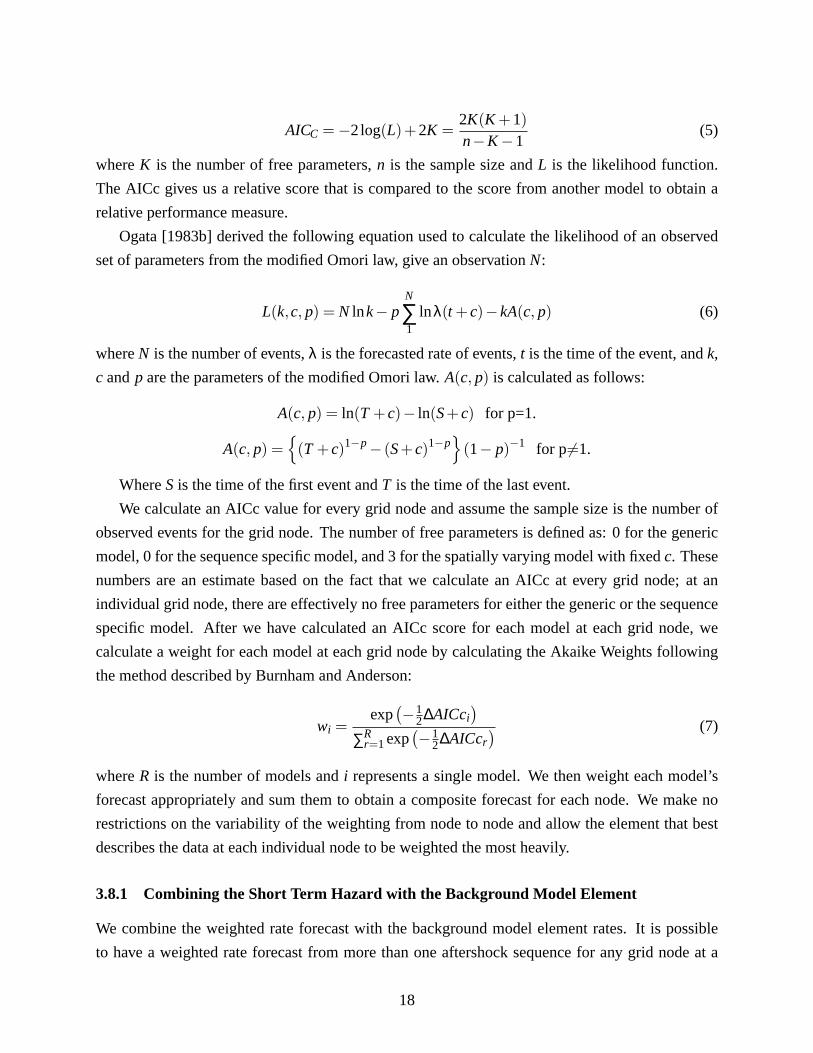
AICC =−2log(L)+2K =2K(K +1)n−K−1

(5)

whereK is the number of free parameters,n is the sample size andL is the likelihood function.

The AICc gives us a relative score that is compared to the score from another model to obtain a

relative performance measure.

Ogata [1983b] derived the following equation used to calculate the likelihood of an observed

set of parameters from the modified Omori law, give an observationN:

L(k,c, p) = N lnk− pN

∑1

lnλ(t +c)−kA(c, p) (6)

whereN is the number of events,λ is the forecasted rate of events,t is the time of the event, andk,

c andp are the parameters of the modified Omori law.A(c, p) is calculated as follows:

A(c, p) = ln(T +c)− ln(S+c) for p=1.

A(c, p) =

(T +c)1−p− (S+c)1−p

(1− p)−1 for p6=1.

WhereS is the time of the first event andT is the time of the last event.

We calculate an AICc value for every grid node and assume the sample size is the number of

observed events for the grid node. The number of free parameters is defined as: 0 for the generic

model, 0 for the sequence specific model, and 3 for the spatially varying model with fixedc. These

numbers are an estimate based on the fact that we calculate an AICc at every grid node; at an

individual grid node, there are effectively no free parameters for either the generic or the sequence

specific model. After we have calculated an AICc score for each model at each grid node, we

calculate a weight for each model at each grid node by calculating the Akaike Weights following

the method described by Burnham and Anderson:

wi =exp

(−12∆AICci

)

∑Rr=1exp

(−12∆AICcr

) (7)

whereR is the number of models andi represents a single model. We then weight each model’s

forecast appropriately and sum them to obtain a composite forecast for each node. We make no

restrictions on the variability of the weighting from node to node and allow the element that best

describes the data at each individual node to be weighted the most heavily.

3.8.1 Combining the Short Term Hazard with the Background Model Element

We combine the weighted rate forecast with the background model element rates. It is possible

to have a weighted rate forecast from more than one aftershock sequence for any grid node at a

18

single time; therefore we add only the highest forecasted rates at any node to the background.

Additionally, we only add the rate of forecasted events if it is greater than the background rate for

the corresponding node. The steps we follow are: 1) at each node, determine the highest short-term

forecasted rate from all active sequences for that node, 2) subtract the background forecast from

our short-term forecast, 3) set any negative rate to 0, 4) add these new rates to the background.

The decision on when to decide a sequence is no longer active and to no longer continue to

forecast rates based on it is made by comparing the total number of forecasted events (M>5) to

the forecasted number in the background. If this total number drops below the background level,

the sequence is terminated. Because we terminate a sequence when its rates reach the background

level, this method assumes that the background rates are represented in the short term forecasts.

3.9 Calculation of Probabilities of Ground Shaking Exceedance.

Once the forecasted rates of events for each sequence have been estimated, we then calculate the

hazard. The hazard calculation follows the standard practices of PSHA [Cornell, 1968] and for

simplicity we will not discuss it in this report.

Because we wished to present the results to the general public in an accessible form we follow

the example of ShakeMaps and use Modified Mercalli Intensity [Wood and Neumann, 1931] for

the final presentation. Level VI was chosen because it is when objects are thrown off shelves so

that the public considers it damaging. To get from PGA to MMI we use the relationship from

Wald, et. al., [1999a]:

Imm= 3.66log(PGA)−1.66 (8)

and derive PGA .126 as a proxy for MMI VI. Thus, we calculate a mean probabilistic seismic

hazard (PSHA) map that gives the log probability of exceeding PGA .126 within a given time

period (24 hours).

Currently we treat all events as point sources for the hazard calculations. The limitation of this

is that source-receiver distances may not be adequately represented for the attenuation calculations.

As this is a common problem for grid-based hazard algorithms, we will be working with RELM

and OpenSHA for an acceptable solution.

For events of magnitude 5.5 and greater we have chosen to apply the Boore, Joyner and Fumal

attenuation relationship [Boore et al., 1997] with the standard PGA coefficients and assuming a

rock site. However, for the relatively low level of hazard that we are interested in, events as small

as magnitude 4 can potentially contribute to hazard and we wish to include them in the calculations.

Therefore, for events between magnitudes 4 and 5 we use a set of coefficients derived from small

California mainshocks [Quitoriano, 2003] and apply a linear smoothing between the two from

19

b1 b2 b3 b5 bv h Va Vs σM < 5.5 2.4066 1.3171 0 -1.757 -0.473 6 760 620 .52M ≥ 5.5 -0.313 0.527 0 -0.778 -0.371 5.57 1396 620 .52

Table 2: coefficients used in the BJF attenuation relationship [Quitoriano, 2003] .

magnitude 5 to 5.5 (table 2).

3.10 Processing Flow Chart

The following section describes the steps that are followed each time the code is triggered. The

current and tested version of the code is written primarily as a suite of Matlab [reference] functions,

with the reliance on several Linux scripts and C language programs for controlling the real time

operations. Rigorous validation of the code has been limited at the time of publication; however

the next generation of the code is currently being written in Java to allow easy interfacing with

validated methods provided by OpenSHA [Field, et. al., 2003]. Translation of the code into Java

will also allow for full validation of the code by comparing results of the Java implementation to

those of the Matlab version.

1. EveryN minutes launch the hazard code. Currently the code takes approximately 10 minutes

to create either a southern or northern California map and is re-launched every 15 minutes.

2. Load scratch files (Sec. 13.(a)) that contain the details from the previous execution of the

code. Specifics included in the scratch files are as follows:

(a) all events from the previous code execution that generated a forecasted rate of events

(M ≥ 5 only) anywhere greater than the background rate for the same location: hence-

forth referred to as previous events.

(b) all aftershocks which were previously assigned to a mainshock (previous event) and

flagged as such.

(c) the seismicity parameters (k,b,c & p) that were assigned to previous events/sequences

(overall sequence including each grid node) in the last code execution.

3. Load all events delivered by QDDS since the previous execution of the code. Perform error

checking to remove duplicate events and correct updated events.

4. Load the gridded background daily rate map (background model element).

20

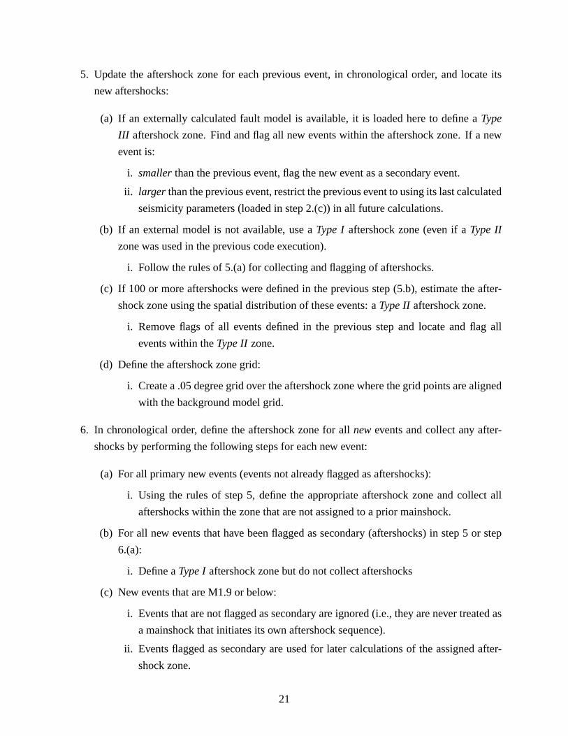
5. Update the aftershock zone for each previous event, in chronological order, and locate its

new aftershocks:

(a) If an externally calculated fault model is available, it is loaded here to define aType

III aftershock zone. Find and flag all new events within the aftershock zone. If a new

event is:

i. smallerthan the previous event, flag the new event as a secondary event.

ii. larger than the previous event, restrict the previous event to using its last calculated

seismicity parameters (loaded in step 2.(c)) in all future calculations.

(b) If an external model is not available, use aType I aftershock zone (even if aType II

zone was used in the previous code execution).

i. Follow the rules of 5.(a) for collecting and flagging of aftershocks.

(c) If 100 or more aftershocks were defined in the previous step (5.b), estimate the after-

shock zone using the spatial distribution of these events: aType IIaftershock zone.

i. Remove flags of all events defined in the previous step and locate and flag all

events within theType IIzone.

(d) Define the aftershock zone grid:

i. Create a .05 degree grid over the aftershock zone where the grid points are aligned

with the background model grid.

6. In chronological order, define the aftershock zone for allnewevents and collect any after-

shocks by performing the following steps for each new event:

(a) For all primary new events (events not already flagged as aftershocks):

i. Using the rules of step 5, define the appropriate aftershock zone and collect all

aftershocks within the zone that are not assigned to a prior mainshock.

(b) For all new events that have been flagged as secondary (aftershocks) in step 5 or step

6.(a):

i. Define aType Iaftershock zone but do not collect aftershocks

(c) New events that are M1.9 or below:

i. Events that are not flagged as secondary are ignored (i.e., they are never treated as

a mainshock that initiates its own aftershock sequence).

ii. Events flagged as secondary are used for later calculations of the assigned after-

shock zone.

21

7. Estimating the overallMc for an aftershock sequence:

(a) If more than 100 events have occurred past .2 days in a sequence, flag all events before

.2 days to be ignored in theMc and parameter calculations. (Note: in the case that

this results in too few events to be used in subsequent calculations (8.b.i & 8.c.i), these

events arenot added back in).

(b) Calculate theMc for each aftershock sequence and flag all events below the estimated

magnitude so they are ignored in later steps. (Note: the spatially varying model element

requires an additional completeness estimation. See step 8(c).iii.)

8. The forecast model elements. For each sequence calculate a grid of seismicity parameters

and rates based on each of the three model elements, if possible:

(a) Generic California model element (Note: a secondary aftershock is limited to using

only this element):

i. Calculate a generick value based on the generica andb values and the forecast

magnitude range of interest.

ii. Spatially smoothk over the grid and assign a smoothed value to each grid cell.

iii. Assign the genericb, c andp values to all cells.

iv. Calculate a forecasted rate of events, for the time period of interest, for each node

based on Equation 3.

(b) Sequence specific model element.

i. Only calculate if more than 100 events aboveMc have been recorded in the se-

quence

ii. Estimate seismicity parametersb, pandk for the sequence. Fixc to .05.

A. If the p value is undetermined, increaseMc by .1 and flag (and ignore) all

events below this magnitude. Repeat until ap value can be estimated or until

fewer than 100 events remain that are greater thanMc. In the latter case, the

sequence specific model element will not be not used.

iii. Spatially smoothk over the grid and assign a smoothed value to each grid cell.

iv. Assign the estimatedb, pandc values to each cell.

v. Calculate a forecasted rate of events, for the time period of interest, for each node

based on Equation 3.

(c) Spatially varying model element.

22

i. Only calculate if more than 100 events aboveMc have been recorded in the se-

quence

ii. Select events within the given radius from each grid node. The radius definition is

given in table 1.

iii. CalculateMc for each grid node, using only the events selected in the previous

step. Flag all events withM < Mc so they are ignored in the next step.

iv. Estimatek, p andb for each grid node;c is fixed to .05. Ignore grid nodes with

fewer than 100 events remaining after the previous step

v. Calculate a forecasted rate of events, for the time period of interest, for each node

based on Equation 3.

9. Model element selection and composite model creation.

(a) For each sequence, for the time since the mainshock to the current time, find the ob-

served number of events in each magnitude bin within each grid cell.

(b) Calculate the likelihood for each model element for each grid cell based on thek, c and

p values and the observed number of events.

(c) Calculate the Akaike Information Criterion for each grid cell for each model element.

(d) Using Akaike Weighting calculate a weight for each model element for each grid cell.

(e) Create a composite forecast for each grid cell by applying the model weights to each

respective rate forecast and summing them.

10. Maximum rate calculation.

(a) For every grid cell on the map find the maximum forecasted rate based on the forecasts

from all mainshocks, secondary events and the background; retain only the highest

forecasted rate at each node.

11. Create a total forecast map.

(a) For each grid cell add the number of forecasted events, above the background level, to

the background. This is done individually for each magnitude bin.

12. Calculate the hazard map using the background map grid.

(a) Calculate the forecasted ground acceleration at each node using the composite forecast.

This is done using the Boore, Joyner, Fumal attenuation relationship (see previous

section for a description of the method).

23

(b) Calculate the probability of exceeding .126g for each grid cell (see previous section for

a description of the method).

13. Write scratch files.

(a) For each grid cell save all events that initiate a forecasted rate of events (M > 5) greater

than the background forecast for the same cell. Also retain, for the overall sequence

and for each grid node, all seismicity parameters (k, b, c & p). Finally, all aftershocks

to the event are retained.

14. Generate the hazard map image

(a) Currently we create a single map for all of California. The map is automatically up-

dated twice an hour: once every 30 minutes. An example map created on August 2,

2004 is shown in figure 8.

4 Model Validation

Main [1999] introduced a 4 level sliding scale of earthquake prediction ranging from time-independent

hazard (standard probabilistic seismic hazard maps), to deterministic prediction (where the loca-

tion, time and size of an earthquake are reliably known ahead of time). The model we evaluate

here falls under Main’s second level category: time-dependent hazard. That is to say, we pro-

pose a degree of predictability based on the modified Omori law [Utsu, et. al., 1995] and the

Gutenberg-Richter relationship (Gutenberg and Richter, 1954] but do not purport to know any par-

ticular features of an event that would upgrade the information to a higher level prediction. For the

purpose of this report, we will refer to our predictions as forecasts.

The aims of statistical testing are to verify a particular forecast model and to ensure that its

results are repeatable and not purely random. This is necessary if one wishes to understand if their

model performs as desired or exhibits any unexpected behavior. Via rigorous statistical testing,

the trap of unwittingly conditioning the data or testing to serve the modelers needs can be avoided

[Console, 2001]. Typically, and in our case, any sort of forecast or prediction has ultimate goals

in providing information to the public. This entails a responsibility of accuracy in the information

that can only be ensured through statistical testing and model validation.

In our case, model validation includes tests providing two distinctly different types of informa-

tion. First we wish to test our model against an established null hypothesis and second we seek

to see if any statement can be made about the consistency of our model with observed data. The

24

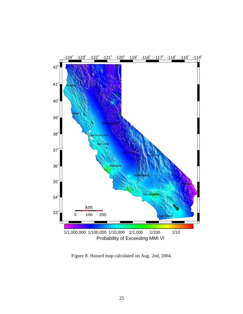
-124˚ -123˚ -122˚ -121˚ -120˚ -119˚ -118˚ -117˚ -116˚ -115˚ -114˚

33˚

34˚

35˚

36˚

37˚

38˚

39˚

40˚

41˚

42˚

0 100 200

km

1/1,000,000 1/100,000 1/10,000 1/1,000 1/100 1/10

Probability of Exceeding MMI VI

Los Angeles

San Diego

San Jose

San Francisco

LM Long Beach

Fresno

Sacramento

0 LM Riverside

Bakersfield

Eureka

Lone Pine

Needles

Parkfield

0 CB El Centro

Ukiah

0 LM Yosemite Village

Figure 8: Hazard map calculated on Aug. 2nd, 2004.

25

difficulty in the first test is finding an appropriate null hypothesis (for which we use the following

definition: an established and accepted model of the same genre as our model). In the case of

time-dependent hazard, there appears not to be an established null hypothesis. While this leaves

the stage open for us to provide one, it leaves us with somewhat unsatisfactory choices for use in

our testing.

We have chosen as our first null, our background model, the Poissonian USGS hazard map

for California [Frankel, et al, 1997]. As this model does not include any clustering, and in fact

specifically excludes hazard due to aftershocks, it would appear obvious that our clustering model

should easily beat it. However, we can make no quantitative statement before performing a test.

It is entirely possible that an inappropriate time-dependent model could fare worse than a time-

independent model when tested against real data. However, any reasonable model that includes

clustering should be favorable.

The next logical null hypothesis is the Reasenberg and Jones model. Unfortunately, due to a

lack of any sort of spatial information, their model as published is not testable directly against our

model. However with the application of a few assumptions we can create a model that is. We

test against the generic California model as well as the generic California model combined with

parameters estimated for individual sequences (previously defined as a sequence specific model).

In the parameter optimization test we create forecasts based on the different parameter combi-

nations we wish to explore and compare them to earthquake dataa posteriori. This allows us to

select the best parameter set based on current knowledge. We describe these assumptions in a later

section.

4.1 Testing Methodology

In cooperation with members of the RELM group, we have participated in the development

of a suite of statistical tests to be used in the testing of earthquake forecasts [Schorlemmer, et al,

in prep]. In this section we describe the two RELM tests that we have used in this study. The

foundation of both tests that we conduct is the likelihood. A widely used statistic, the likelihood

is somewhat similar to the residual sum of squares method in that it gives a value related to the

consistency of a model and its parameters to observations. However, instead of giving a norm of

residuals between the observations and the model it gives theprobability densityof making those

particular observations given the model parameters. A likelihood, therefore, gives an indication of

how consistent a model is with the data.

The two tests we discuss here are:

• Consistency test:likelihoods calculated using instrumental data and simulations. In this test

we investigate how well our hypothesis fits the data and if we can reject the hypothesis with

26

the given significance. This test is designed to answer the question of how well does our

hypothesis do at forecasting real data.

• Ratio test: likelihoods calculated using instrumental data and simulations; this test investi-

gates if one hypothesis can be rejected in favor of another with the given significance. An

important question in the design of our hypothesis is whether the addition of complexity(e.g.

spatial variations in theb value) improves the forecasts over a more simple hypothesis. The

ratio test is designed to answer this question.

We test the forecasted rates of events rather than the forecasted probabilities of ground motion, for

two reasons. Calculating forecasted ground motions adds a large amount of uncertainty (due to the

attenuation relationship, site and source characteristics) to the forecast and we do not wish to have

this uncertainty obscure our actual rate forecast. Additionally, the data that would be necessary for

performing retrospective tests of ground motion is very limited.

An unbiased test of forecasted rates would be to calculate a rate forecast for a future time, wait

for this time to pass and then test how the model did by calculating a likelihood. Unfortunately

it can take a long time before enough events have occurred so that one can obtain a strong result.

We approach this problem by using historical data and performing retrospective tests. However, as

part of the RELM group, prospective tests will be initiated in the near future.

The likelihood value is a measure of the probability that a similar result would be obtained

under a given hypothesis, and for that we need a probability distribution of earthquake numbers in

a given region. Many seismological studies assume a Poisson processs, in which the earthquake

rate is constant in time, independent of past events. However, Michael [1997] and others question

its validity for earthquake occurrence, and the Poisson process is inconsistent with clustering.

Nevertheless, for short enough time intervals the earthquake rate may not vary too much, and the

Poisson process may be a good approximation as long as the rate is re-evaluated for each time

interval. A generalized Poisson process for which the basic rate depends on time is known as a

non-stationary Poisson process.

A simple likelihood alone is not sufficient; if we wish to make a statement about the consis-

tency of our model with the data or when comparing our model to another model with the goal of

rejecting, we must be able to attach a significance to this statement. We must be able to say that

the results we have obtained are not simply due to random chance and that in another situation the

results would be similar [Joliffe and Stefanson, 2003]. We therefore need a probability distribution

of likelihood scores. Unfortunately, an analytical derivation of this is not practical and we must

generate it through simulations.

To simulate catalogs, we must first create our forecast for the test period. The forecast must

27

include the expected number of events for each magnitude (4<M<8) and location being tested. We

then assume there is a random probability governed by the Poisson distribution for a number of

events to occur in each magnitude-space bin that is other than the forecasted number and draw a

simulated number of events for each magnitude and location. This is done for two reasons: 1)

because we wish to gain insight into how our model is performing and do not wish to perform a

binary test where a forecasted event is 100% correct or 100% wrong; and 2) because our model

provides a probability of events occurring and not an exact whole number of forecasted events (e.g.,

for the time period of interest we might forecast .1 events for a given magnitude in a particular grid

cell). This allows us to calculate a distribution of earthquakes that is theoretically consistent with

the model but that also allows for the random Poissonian scatter that is implied in the model. For

each bin we calculatemanysimulations (typically 1,000) and obtain a likelihood for each, resulting

in a distribution of likelihoods.

If the likelihood of the observed data occurs in the lower 5% tail of this distribution, then

the observation is unlikely to occur in the model, and therefore the model can be rejected with a

significance of 5%. Thus there is less than a 5% chance that we would reject a true hypothesis.

In our simplest test, a consistency test, we simulate earthquakes that obey the assumptions of

the hypothesis being tested, calculate the likelihood scores for these simulations and then compare

them to the likelihood of the observed data. If the tested hypothesis is consistent with the observed

data, the likelihood of the observed data should not fall among the outliers of the distribution of

the simulated likelihoods but should be clearly within the distribution.

The procedure for the ratio tests is similar to the method used for the consistency test. One

important difference is that we calculate the ratio of the likelihood of the null hypothesis over the

likelihood of the alternative hypothesis. This allows us to investigate whether we can reject the

null hypothesis in favor of the alternative hypothesis, and if so attach a significance to the result.

Because we simulate earthquakes based on the null hypothesis only, there are just two possible

outcomes: rejection of the null hypothesis, or no rejection of the null hypothesis.

The ratio test only compares the two hypotheses; it does not test whether either is truly con-

sistent with the data. If the null hypothesis is rejected, it may happen that both hypotheses are

consistent (by the consistency test above), or that only the alternative hypothesis is consistent, or

that both are inconsistent.

4.1.1 Test Calculations

In testing a forecast, we require the forecast to be specified as an earthquake rate per area, time

and magnitude bin. The simplest way to test the model is to use a grid based test. Therefore,

to remain consistent with the resolution of our forecast, we test on the same grid as we use to

initially create the forecast, a.05 X .05 grid. In order to reduce the computational expense, we

28

currently perform only one test per day. This unfortunately limits the resolution of our results.

In the initial time period after a large mainshock, the production of aftershocks decreases very

quickly; a substantial reduction in earthquake rate will occur within the first 24 hours. Due to

using large time steps we integrate this change over a longer period and potentially miss testing

the ability of our model to correctly forecast these temporal changes. Ideally we would test more

frequently or only at the time of event occurrence. However due to the computational limitations

mentioned above we were unable to do so in this study.

We denote each binb as a subset of total set of binsB :

B := b1,b2, . . . ,bn,n = |B| (9)

wheren is the number of binsbi in the setB. For each bin, we have a forecasted rate of events

λiwith the total forecasted rate defined as:

Λ =

λ1

λ2...

λn

,λi := λi(bi),bi ∈ B. (10)

We bin the observed events,ωi , in the same manner as above resulting in:

Ω =

ω1

ω2...

ωn

,ωi = ωi(bi),bi ∈ B. (11)

As stated previously, we assume that for the time period of each test, earthquakes are independent

of each other. This allows us to calculate the probability, given the forecasted rateλ, of observing

ω events per bin based on the Poissonian probability:

p(ω|λ) =λω

ω!e−λ. (12)

The log-likelihoodL for observingω earthquakes from a given forecasted rateλ is defined as the

logarithm of the probabilityp(ω|λ):

L(ω|λ) = logp(ω|λ) =−λ+ω logλ− logω! (13)

for each individual bin. From this we can obtain the total log-likelihood for all bins by calculating

29

the log of the product of all probabilities (the joint probability):

L(Ω|Λ) =n

∑i=1

L(ωi|λi) =n

∑i=1−λi +ωi logλi− logωi ! (14)

This is the log-likelihood we use for the consistency test. To compare two models, we must com-

pute the log-likelihood-ratio:

R= L(Ω|Λ0)−L(Ω|Λ1) = L0−L1 (15)

whereΛ0 is the forecasted rates of hypothesisH0andΛ1 is the forecasted rates of hypothesisH1.

L0 andL1 are the respective hypothesis joint probabilities. IfR≤ 0 , H1 provides a more likely

forecast; ifR≥ 0, H0 is more likely.

4.1.2 Simulations

Assuming a Poisson distribution, each forecasted number of events has a probability of some other

number of events occurring consistent with the forecasted number. We use this probability to

randomly draw a number of events, for each bin, to create a simulated catalog that is consistent

with the forecast. Therefore we are able to obtain a probability distribution of log-likelihood

scores for this hypothesis. By comparing the log-likelihood based on the observed events to the

distribution of simulated likelihoods, we are able to see how likely it is to observe the real events

in the hypothesis. By investigating where the observed log-likelihood falls in the distribution of

simulated log-likelihoods, we are able to attach a significance to the observed result. For example,

if the observed log-likelihood falls in the lower 5% of the simulated log-likelihoods, we can reject

the hypothesis.

By randomly drawing from the inverse cumulative Poissonian probability density function we

obtain thesimulatedobserved eventsωi for each given bin. Doing this for all bins, we obtain the

total number of simulated events:

Ω j =

ω j1

ω j2...

ω jn

, ω ji = ω j

i (bi),bi ∈ B

Ω jk where j denotes which hypothesis forecast was used andk corresponds to an individual simu-

lation run.

30

4.1.3 Consistency test

In this test we wish to know if we can reject our hypothesis as being consistent with the data.

Before we are able to do this, it is up to us to define the significance levelα at which we will reject

the model. The standard in the literature is typically either 0.05 or 0.01; we have chosen to use

α = 0.05.

The significance is defined as the fraction of simulated log-likelihoods that are less than the

observed log-likelihood:

γ =|Lk|Lk ≤ L, Lk ∈ L|

|L | (16)

Here Lk denotes the log-likelihood of thekth simulation. If γ is less than 0.05 we can state that

the hypothesis is inconsistent with the data and reject it with with a significance of 0.05. Ifγ is

greater than 0.05 we conclude the hypothesis is consistent with the data based on this this particular

measure.

4.1.4 Ratio Test

The ratio test allows us to investigate if we can reject the null hypothesis,H0,based on the alter-

native hypothesis,H1. To do this, we must first calculate the log-likelihood for each hypothesis

based on the observations and then calculate the ratioR of these values:

R= L(Ω|Λ0)−L(Ω|Λ1) (17)

Additionally, we calculate a ratio for every simulated data set,k, resulting in a distribution of

log-likelihood ratios:

Rk = L(Ω0k|Λ0)−L(Ω0

k|Λ1) (18)

Significance and rejection are determined using the same method as used in the consistency test

and usingα = .05.

4.2 The Data

All earthquake data that we used in the testing comes from the Southern California Earthquake

Data Center. The overallMc for the time period we test is claimed to be 1.8, however the actual

value is much higher following large mainshocks. The majority of the events are reported to have

horizontal location errors of±1km and depth errors of±2km; however occasionally events are

report with both errors at greater than 5km. Magnitude errors are not reported. Location errors of

31

less than 5km have little effect on our eventual forecast due to the large smoothing radius we use

when calculating the seismicity parameters. Better locations would, however, allow us to increase

our spatial resolution and potentially create more accurate forecasts. Twenty-four hours following

the Landers mainshock, we implement an external fault model. This model is the surface projection

of the fault rupture model of Wald and Heaton [1994].

4.3 Results

When the testing procedures are coupled with the time-dependent hazard analysis, the calculation

becomes very computationally expensive. This expense is compounded when simulations are used.

Additionally, time periods where large aftershock sequences are present (1992 - present for south-

ern California) proceed much more slowly than times where few active sequences are present. With

the implementation of a computing system designed just for these sorts of problems by RELM, the

computation speed should improve markedly. Unfortunately, until that system becomes available,

we are limited to performing our test less often and for fewer cumulative years than is desirable.

All tests consisted of daily computed 24 hour rate forecasts that we compared with the observed

earthquake numbers and locations for the identical time period. We initiated all tests on January 1,

1992. However, due to different needs for different tests, i.e., different number of tested parameter

sets, some tests were able to run longer than others.

For all tests other than the ratio test against the generic model element, 1,000 simulations were

used. Due to time and computational constraints, for the generic test, we used only 100; this is

not wholly satisfactory, however the results are strong enough to warrant additional simulations

unnecessary.

4.4 Ratio and Consistency Testing

The following two tests, measure the consistency of our model with the observed data and the

relative consistency of another model as compared to ours.

4.4.1 Consistency Test Results

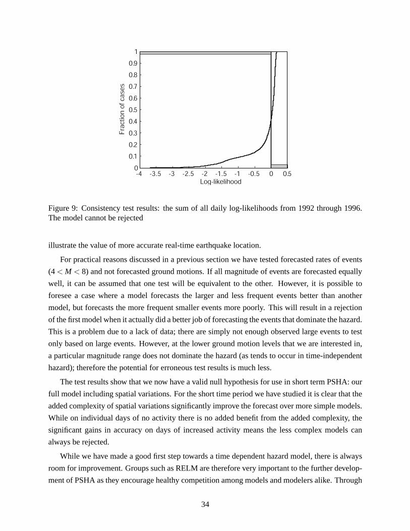
This test was the run from the beginning of 1992 to the end of 1996 using our full model; regionally

we tested all of southern California. When calculating a log-likelihood for each 24 hour period and

summing all log-likelihood values, the model performed well and could not be rejected. The model

was consistent and could not be rejected on days with many earthquakes (M>4) or on days with

few to none.

32

How to read the S plots: Each plot displays two likelihoodscores:

1) the S-curve is the cumulative distribution of the log-likelihoods based on the simulations.

An individual point on the S-curve represents the fraction of overall simulations that

obtained a particular log-likelihood score.

2) the log-likelihood of the observed data. All plots are normalized so that the observed

log-likelihood is 0.

If the observed log-likelihood (0 line) falls in the middle of the simulated log-likelihoods the

model is consistent with the data. If the observed is to the left of the simulations (a lower score)

it is not among the simulated likelihood scores and is therefore not likely to occur in the model.

The grey bar represents the 5% rejection area. If any portion of the S-curve touches this

line, it may be rejected.

4.4.2 Background, Generic and Sequence Specific Ratio Tests

Using the same region as above, but using approximately 3 years of data, we performed three

log-likelihood ratio tests where the full composite model was the alternative hypothesis. In each

test we used a different null hypothesis: 1) Poissonian background model, 2) generic California

model defining an aftershock zone as the area within one Wells and Coppersmith fault length of

the mainshock, and 3) a composite model including the generic and sequence specific models

(allows for multiple fault models, etc.). The results of the ratio test were consistent in all three

tests; the null hypothesis can be rejected with a significance of .05 (fig. 10). On individual days

where there where no observed events, the null hypotheses could often not be rejected due to very

similar likelihood scores between the models. However on days where events were observed, the

alternative hypothesis consistently had significantly higher likelihood scores resulting in the overall

rejection of each null hypothesis.

5 Discussion and Conclusions

So far our testing has been retrospective, using revised earthquake catalogs. The revised catalogs

include corrected locations and magnitudes, and they may take months to be released. Thus our

test results are optimistic for two reasons. First, as with any retrospective test, we have the oppor-

tunity to make adjustments to the model that would not be possible in a real-time, prospective test.

Second, we use corrected data that would not be available in a real time exercise. Location and

magnitude errors, and the presence of phantom events that are later edited out of the catalog, could

spoil a predictive relationship. We will proceed with a prospective test soon under the RELM

project. Should we find a significant improvemet in results based on corrected data, that would

33

-4 -3.5 -3 -2.5 -2 -1.5 -1 -0.5 0 0.50

0.1

0.2

0.3

0.4

0.5

0.6

0.7

0.8

0.9

1

Fra

ctio

n o

f ca

ses

Log-likelihood

Figure 9: Consistency test results: the sum of all daily log-likelihoods from 1992 through 1996.The model cannot be rejected

illustrate the value of more accurate real-time earthquake location.

For practical reasons discussed in a previous section we have tested forecasted rates of events

(4 < M < 8) and not forecasted ground motions. If all magnitude of events are forecasted equally

well, it can be assumed that one test will be equivalent to the other. However, it is possible to

foresee a case where a model forecasts the larger and less frequent events better than another

model, but forecasts the more frequent smaller events more poorly. This will result in a rejection

of the first model when it actually did a better job of forecasting the events that dominate the hazard.

This is a problem due to a lack of data; there are simply not enough observed large events to test

only based on large events. However, at the lower ground motion levels that we are interested in,

a particular magnitude range does not dominate the hazard (as tends to occur in time-independent

hazard); therefore the potential for erroneous test results is much less.

The test results show that we now have a valid null hypothesis for use in short term PSHA: our

full model including spatial variations. For the short time period we have studied it is clear that the

added complexity of spatial variations significantly improve the forecast over more simple models.

While on individual days of no activity there is no added benefit from the added complexity, the

significant gains in accuracy on days of increased activity means the less complex models can

always be rejected.

While we have made a good first step towards a time dependent hazard model, there is always

room for improvement. Groups such as RELM are therefore very important to the further develop-

ment of PSHA as they encourage healthy competition among models and modelers alike. Through

34

-200 0 200 400 600 800 1000 12000

0.1

0.2

0.3

0.4

0.5

0.6

0.7

0.8

0.9

1

--500 0 500 1000 1500 2000 2500 30000

0.1

0.2

0.3

0.4

0.5

0.6

0.7

0.8

0.9

1

Figure 10:Left : Ratio test for 1992-1994 of generic California model (test 2) against the compositemodel. Generic model is rejected with a significance of .05.Right: Ratio test for 1992-1995 ofcomposite model excluding any spatially varying information (test 3) and the full composite model.The model without spatially varying information can be be rejected with a significance of .05.

the use of tools that will become available to us in the near future via RELM we will address the

questions listed above through much more extensive testing of our own model against itself as well

as against other time-dependent models. An important contribution of this will be the organization

of real-time prospective testing that is a necessary component of any complete statistical forecast

testing routine [Console, 2001].

Acknowledgments

We thank Ned Field, David Jackson for their helpful reviews and comments; Danijel Schorlemmer

for his numerous discussions and input into the development of the processing scheme; and Stan

Schwarz and Jan Zeller for their assistance in setting up the necessary IT support to be able to

operate in real time.

References

Aki K., Maximum likelihood estimate ofb in the formulalogN = a−bM and its confidence limits,

Bull. Earthq. Res. Inst., 43, 237-239, 1965.

Boore, D.M., W.B. Joyner, and T.E. Fumal, Equations for estimating horizontal response spectra

and peak acceleration from western North America earthquakes: A summary of recent work,

Seismological Research Letters, 68, 128-153, 1997.

Bufe, C.G., and D.J. Varnes, Time-to-failure in the Alaska-Aleutian region: an update, EOS, 77

(F456), 1996.

35

Burnham, K.P., and D.R. Anderson, Model Selection and Multimodel Inference A Practical Information-

Theoretic Approach, Springer-Verlag, 2002.

Console, R., Testing earthquake forecast hypothesis, Tectonophysics, 338, 261-268, 2001.

Cornell, C.H., Engineering seismic risk analysis, Bulletin of the Seismological Society of Amer-

ica, 58, 1583-1606, 1968.

Enescu, B.a.I., K., Some premonitory phenomena of the 1995 Hygo-ken Nanbu Earthquake: seis-

micity b-value and fractal, Tectonophys., 338(3-4), 297-314, 2001.

Felzer, K., R.E. Abercrombie, and G. Ekstrom, A common origin for aftershocks, foreshocks, and

multiplets, submitted Bulletin of the Seismological Society of America, March, 2003.

Field, E.H., Jordan, T.H., and Cornell, C.A., OpenSHA: A developing community-modeling en-

vironment for seismic hazard analysis, Seismological Research Letters, 74, 2003.

Frankel, A., C. Mueller, T. Barnhard, D. Perkins, E.V. Leyendecker, N. Dickman, S. Hanson,

and M. Hopper, National seismic hazard maps, United States Geological Survey Open-File

Report, 96-532, 1996.

Frankel, A., C. Mueller, T. Barnhard, D. Perkins, E.V. Leyendecker, N. Dickman, S. Hanson, and

M. Hopper, Seismic hazard maps for California, Nevada and western Arizona/Utah, United

States Geological Survey Open-File Report, 97-130, 1997.

Frohlich, C., and S. Davis, Teleseismicb-Values: Or, Much Ado about 1.0, Journal of Geophysical

Research, 98, 631-644, 1993.

Giardini, D., The Global Seismic Hazard Assessment Program (GSHAP) - 1992/1999, Annali de

Geofisica, 42, 957-974, 1999.

Gutenberg, B., and C.F. Richter, Magnitude and energy of earthquakes, Ann. Geofis., 9, 1-15,

1954.

Harris, R., Introduction to special section: Stress triggers, stress shadows, and implications for

seismic hazard, Journal of Geophysical Research, 103, 24347-24358, 1998.

Jackson, D., and Y. Kagan, Testable earthquake forecasts for 1999, Seismological Research Let-

ters., 70, 393-403, 1999.

Ji, C., D.J. Wald and D.V. Helmberger, Sip history of the 1999 Hector Mine, California earthquake,

Seismological Research Letters, 71, 224, 2000.

36

Jolliffe, T., and Stephenson, Forecast verification, a practitioner’s guide in atmospheric science,

Wiley, 2003.

Kagan, Y.Y., and D. Jackson, Probabilistic forecasting of earthquakes, Geophys. J. Int., 143, 438-

453, 2000.

Main, I., Is the reliable prediction of individual earthquakes a realistic goal? Nature online debates,

http://www.nature.com/nature/debates/earthquake ,1999.

Matsu’ura, R.S., Precursory quiescence and recovery of aftershock activity before some large af-

tershocks, Bull. Earthq. Res. Inst., 61, 1-65, 1986.

Michael, A., Testing prediction methods: earthquake clustering versus the Poisson model, Geo-

physical Research Letters, 24, 15, 2997.

Ogata, Y., Estimation of the parameters in the modified Omori formula for aftershock frequencies

by the maximum likelihood procedure, J. Phys. Earth, 31, 115-124, 1983a.

Ogata, Y., Estimation of the parameters in the modified Omori fornula for aftershock frequencies

by the maximum likelihood procedure, J. Phys. Earth, 31, 115-124, 1983b.

Ogata, Y., Detection of precursory relative quiescence before great earthquakes through a statisti-

cal model, Journal of Geophysical Research, 97, 19845-19871, 1992.

Ogata, Y., Seismicity Analysis through Point-process Modeling: A Review, Pure and Appl. Geo-

phys, 155, 471-507, 1999.

Quitoriano, V., personal communication, 2003.

Reasenberg, P.A., Second-order moment of central California seismicity, 1969-1982, 90, B7,

5479-5495, 1985.

Reasenberg, P.A., Computer Programs ASPAR, GSAS and ENAS and APROB for the Statistical

Modeling of Aftershock Sequences and Estimation of Aftershock Hazard, U.S. Geological

Survey Open-File Report, 1994.

Reasenberg, P.A., and L.M. Jones, Earthquake hazard after a mainshock in California, Science,

243, 1173-1176, 1989.

Reasenberg, P.A., and L.M. Jones, California aftershock hazard forecast, Science, 247, 345-346,

1990.

37

Reasenberg, P.A., and L.M. Jones, Earthquake aftershocks: Update, Science, 265, 1251-1252,

1994.

Reasenberg, P.A., Foreshock occurrence before large earthquakes, Journal of Geophysical Re-

search, 104, 4755-4768, 1999.

Schorlemmer, D., D. D. Jackson, and M.C. Gerstenberger, Earthquake Likelihood Model Testing,

in prep, 2003.Stein, R.S., G.C.P. King, and J. Lin, Change in failure stress on the San An-

dreas and surrounding faults caused by the 1992 M=7.4 Landers earthquake, Science, 258,

1328-1332, 1992.

Sieh, et al....

Utsu, T., Ogata, Y., & Matsu’ura, R. S., The centenary of the Omori formula for a decay law of

aftershock activity, Journal of the Physics of the Earth, 43, 1-33, 1995.

Wald, D.J. and Heaton, T.H., Spatial and temporal distribution of slip for the 1992 Landers, Cali-

fornia, earthquake. Bulletin of the Seismological Society of America, 84, 668-691, 1994.

Wald, D.J., V. Quitoriano, T.H. Heaton, and H.Kanamori, Relationships between peak ground

acceleration, peak ground velocity and Modified Mercalli Intensity in California, Earthquake

Spectra, 15, 557-564, 1999a

Wald, D.J., V. Quitoriano, and T.H. Heaton, TriNet “ShakeMaps”: Rapid Generation of Instru-

mental Ground Motion and Intensity Maps for Earthquakes in Southern California, Earth-

quake Spectra, 15, 537-556, 1999b.

Wells, D.a.C., K. Coppersmith, New emperical relationships among magnitude, rupture length,

rupture width, rupture area, and surface displacement, Bulletin of the Seismological Society

of America, 84, 974-1002, 1994.

Wiemer, S., Introducing probabilistic aftershock hazard mapping, Geophysical Research Letters,

27, 3405-3408, 2000.

Wiemer, S., Gerstenberger, M., Hauksson, E., Properties of the Aftershock Sequence of the 1999

Mw 7.1 Hector Mine Earthquake: Implications for Aftershock Hazard, Bulletin of the Seis-

mological Society of America, 92 (4), 2002.

Wiemer, S., and K. Katsumata, Spatial variability of seismicity parameters in aftershock zones,

Journal of Geophysical Research, 104, 13,135-13,151, 1999.

38

Wiemer, S., and M. Wyss, Mapping the frequency-magnitude distribution in asperities: An im-

proved technique to calculate recurrence times?, Journal of Geophysical Research, 102,

15115-15128, 1997.

Wiemer, S., and M. Wyss, Minimum magnitude of complete reporting in earthquake catalogs:

examples from Alaska, the Western United States, and Japan, Bulletin of the Seismological

Society of America, 90, 859-869, 2000.

Wood, H.O., and F. Neumann, Bulletin of the Seismological Society of America, 21 (4), 277-283,

1931.

Wyss, M., Cannot earthquakes be predicted?, Science, 278, 487-488, 1997.

39