Real time digital audio processing using Arduino

Andre Jucovsky BianchiComputer Science Department

University of Sao Pauloajb@ime.usp.br

Marcelo QueirozComputer Science Department

University of Sao Paulomqz@ime.usp.br

ABSTRACT

In the search for low-cost, highly available devices forreal time audio processing for scientific or artistic purposes,the Arduino platform comes in as a handy alternative for achordless, versatile audio processor. Despite the fact thatArduinos are generally used for controlling and interfacingwith other devices, its built-in ADC/DAC allows for cap-turing and emitting raw audio signals with very specificconstraints. In this work we dive into the microcontroller’sstructure to understand what can be done and what are thelimits of the platform when working with real time digi-tal signal processing. We evaluate the behaviour of somecommon DSP algorithms and expose limitations and pos-sibilities of using the platform in this context.

1. INTRODUCTION

Arduino is the name of a hardware and software projectstarted in 2005 which aims to simplify the interface ofelectric-electronic devices with a microcontroller [1]. Itevolved from the Processing software IDE 1 (2001) andthe Wiring software and hardware prototyping platform 2

(2003). Hardware, software and documentation designsare published under free licenses (Creative Commons BY-SA 2.5, GPL/LGPL and CC BY-SA 3.0, respectively) anda large community has grown to provide code and supportfor newcomers. Nowadays, many Arduino hardware de-signs are available and range from more limited 8-bit mi-crocontrollers to fully featured 32-bit ARM CPUs. Be-sides, other advantages of Arduino for academic and artis-tic use are its mobility (because of its low power needs andpossibility of running on batteries for hours, if not daysdepending on the use), expandability (because of its stan-dardized interface for attaching so called hardware shields)and price (selling for under 20 US dollars online).

Despite all these advantages, the Arduino platform hasa somewhat limited processing power when compared tostandard processors available in the market, as for exampleDSP chips such as Analog Device’s Blackfin 32-bit RISC

1 http://www.processing.org/2 http://wiring.org.co/

Copyright: c©2012 Andre Jucovsky Bianchi et al. This

is an open-access article distributed under the terms of the

Creative Commons Attribution 3.0 Unported License, which permits unre-

stricted use, distribution, and reproduction in any medium, provided the original

author and source are credited.

processors 3 and FPGA-based processors such as XilinxVirtex-7 family 4 . Research and industry advances haveled to optimized computational performance and power con-sumption for these platforms [2], but we could not find athorough examination of the use of a low-tech device suchas the Arduino.

In this work, we aim to systematically expose the micro-controller-based Arduino platforms’ possibilities for car-rying real time digital audio processing tasks so there canbe more accurate elements to be taken into account whenmaking the choice for a platform. Code examples can bedownloaded from the IME/USP Computer Music Groupwebpage 5 .

1.1 Related work

Arduino has been experimentally used as a real time au-dio processor for sampling audio and control signals withan effective rate of 15.125 KHz [3], which provided thebase for our investigation. Also, an ALSA audio driver wasimplemented to use the Arduino Duemilanove [4] as a full-duplex, mono, 8-bit 44.1 KHz sound card under GNU/Linux.

2. METHODS

In order to meet the needs for real time audio processing,the microcontroller has to be tweaked so we can capture,process and output analog audio. Each of these tasks canbe performed in a variety of ways, and for this examina-tion we chose to go with the basic functionalities of theplatform.

In this investigation, we used an Arduino Duemilanovewith an ATmega328P microcontroller from Atmel, a verymodest version of the platform. It has an 8-bit RISC centralprocessor, operates with a base frequency of 16 MHz, andhas memory capacity of 32 KB for program storage and2 KB for random access [5]. From now on, whenever werefer to the microcontroller, we are in fact talking aboutthis specific model from this specific manufacturer.

2.1 Microcontroller’s elements

To be able to know how to configure the platform to suitour needs, a general understanding of the inner workings ofa microcontroller is needed. The Atmel megaAVR series

3 http://www.analog.com/en/processors-dsp/blackfin/products/index.html

4 http://www.xilinx.com/products/silicon-devices/fpga/virtex-7/index.htm

5 http://compmus.ime.usp.br/en/arduino

538

Proceedings of the Sound and Music Computing Conference 2013, SMC 2013, Stockholm, Sweden

microcontroller is comprised of several components, someof which are fundamental for our investigation and so willbe briefly covered in this section.

2.1.1 Clocks

Many clocks provide the frequencies in which the differentparts of the microcontroller work. They are basically eitheremitters or dividers of square wave signals that provide thefrequency of operation of the CPU, the ADC, the memoryaccess and other components of the microcontroller. Pos-sible sources of clock frequencies are crystal and RC os-cillators.

A useful concept associated with clocks is the one of aprescaler. Prescalers are dividers for clock frequenciesthat either actually lower the frequency of a clock or atleast trigger specific interrupts on a (power of two) frac-tion of a clock’s frequency.

The system clock provides the system’s base frequencyof operation. Other important clocks are the I/O clock andthe ADC clock used for feeding a frequency to most of theinput/output mechanisms. It is possible to choose whichclock will feed a frequency to some parts of the system,as well as select prescaler values independently. In ourstudy, we make use of the timer clock prescaler to controlthe PWM frequency that drives our DSP mechanism, as wewill see in Section 2.3.

2.1.2 Registers and interrupts

The microcontroller’s CPU is comprised of an arithmeticlogic unit that works with 32 registers – portions of me-mory that provide data for computation as well as deter-mine the execution flow of the program. An interrupt is anattempt of deviation from the current execution flow thatcan be triggered by a variety of events in the system, usu-ally by setting reference values on specific registers.

In our case, interrupts are of extreme value as they arethe low level structures that allow us to execute code witha somewhat fixed frequency (at least if we assume that theclock frequencies are indeed constant in relation with realtime).

2.1.3 Timers/counters

A timer, or counter, is a register whose value is automat-ically incremented according to a specific clock. Whena counter hits its maximum value it is reset to zero andsignals an overflow interrupt, which may cause a certainfunction to be called.

Timers are important in the context of DSP because theyprovide a natural way to perform many of the DSP chaintasks, as for example to periodically launch the input signalsampling function (that fills the input buffer) and to emit aPWM square wave which, after analog low-pass filtering(through an integrator), corresponds to a smooth analogsignal. The ATmega328P has two 8 bit counters and one16 bit counter, each having different sets of features but allbeing capable of doing PWM.

2.1.4 Input and output pins

Microcontrollers can receive and emit digital signal throughI/O pins, which in the case of the Arduino board are con-veniently mounted in such a way that it is easy to plugother components and boards. These pins are read fromand written to according to frequencies governed by dif-ferent clocks (I/O, ADC and others).

In principle, the microcontroller pins are designed to workwith binary signals represented by two different voltages(0 V and 5 V with a threshold value to account for small de-viations). Despite that, I/O pins come equipped with handymechanisms for sampling band limited input signals whosevoltages vary between the reference extremes, and alsofor generating waveforms that, after being filtered, outputvarying signals of the same nature. These mechanisms are,respectively, the analog-to-digital converter (ADC) and thepulse-width modulation (PWM), which will be seen in thenext sections.

2.1.5 Memory

The microcontroller has 3 manageable memory spaces forstoring the program and working data, and the followingtable summarizes the different characteristics and purposesfor each type of memory:

Type Size(KB)

Data per-sistency

Write time(clock ticks)

Endurance(write/erasecycles)

Flash 32 yes 1 10,000SRAM 2 no 2 n/a

EEPROM 1 yes 30 100,000

Usually, the Flash memory stores the program, the SRAMmemory stores volatile data used along the computation,and the EEPROM is used for longer-term storage betweenworking sessions. Notice that the amount of SRAM me-mory represents a hard limit for many DSP algorithms. A512 point lookup table filled with precalculated sinewavebytes, for example, represents 25% of all available work-ing space. Thus, it might be interesting to store hardcodeddata in the program memory whenever possible if memoryworking space is lacking.

2.2 Audio in: ADC

Data can flow into the microcontroller in a variety of ways,the most basic being embedded mechanisms for digital se-rial communication and analog-to-digital conversion usingthe input pins. The former mechanism can feed digital datadirectly into memory, while the latter can either read 1 bitfrom an input pin (as explained in the last section) or sam-ple an analog value between the reference voltages using 8or 10 bits resolution.

Rather than providing the microcontroller with digital data,our setup uses the embedded analog-to-digital conversionto sample an audio signal using the microcontroller pins’ADC mechanism. This choice was made so the signal canbe directly connected to the microcontroller (i.e. no exter-nal device has to be used for sampling) and we can study

539

Proceedings of the Sound and Music Computing Conference 2013, SMC 2013, Stockholm, Sweden

the device’s performance taking into account this crucialstep in the digital audio processing chain.

The ADC uses a Sample and Hold circuit that holds theinput voltage at a constant level until the end of the con-version. This fixed voltage is then successively comparedwith reference voltages to obtain a 10 bit approximation.If a faster conversion is desired, precision can be sacrificedand the first 8 bits can be read before the last 2 are com-puted. Conversion time takes between 13 and 250 µs, de-pending on several configuration parameters that influencethe precision of the result.

As noted before, the ADC mechanism has a dedicatedclock to ensure conversion can occur independently of othermicrocontroller parts. Also, the mechanism can be trig-gered manually (on demand) or automatically (a new con-version starts as soon as the last one has finished).

2.3 Audio out: PWM

Once the input signal has been sampled and processed, oneway to convert it back to analog is to use the embeddedpulse-width modulation (PWM) mechanism that is avail-able in some of the output pins of the microcontroller, fol-lowed by an analog filtering stage. A PWM wave encodesa determined value in the width of a square pulse. In or-der to do this, it defines a duty cycle as the percentage oftime that the square wave has its maximum value in rela-tion to the total time between square pulses (see Figure 1).The encoding of a value x ranging from X1 to X2 is justthe enforcement of a duty cycle with a percentage equal tox−X1

X2−X1.

Figure 1. Examples of PWM waves with different dutycycles. The left alignment of the waves corresponds to theFast PWM mode.

The final analog filtering stage is needed to remove highfrequency components present in the square wave spec-trum to reconstruct a band limited signal. In our case, thisfiltering is made from a simple RC integrator circuit thatstands between the output pin and a normal speaker.

The PWM mechanism can operate in different modes whichvary according to how the reference value to be encoded

relates with a counter’s signal to generate the output val-ues of the modulated wave. In Fast PWM mode, the outputsignal is set to 1 in the beginning of the cycle and becomes0 whenever the reference value becomes smaller than thecounter value (see Figure 2). This mode has the disadvan-tage of outputting the square pulses aligned to the left ofthe PWM cycle, and so the Phase correct mode is avail-able to solve this problem at the expense of cutting the sig-nal generation frequency in half. It works by making thecounter count back to zero instead of being reset when ithits its maximum value.

Figure 2. Time evolution of register values in the PWMmechanism. TCNTn is the value of the counter and OCnxis the value of the output pin. Note how changes in thereference value determine the duty cycle on each wave pe-riod.

The output frequency of the PWM signal is a functionof the clock selected to be used as input for the counter,the counter prescaler value, the size of the counter (in bits)and the PWM mode. For a b bits counter with input clockof fclock Hz and prescaler value of p, an output pin con-figured to operate in fast PWM mode overflows with a

frequency offclockp× 2b

Hz. This provides us with a way to

output the processed signal while using the same infras-tructure to schedule periodic actions, such as querying forADC values and signaling that blocks of samples are readyto be processed.

Also notice that the counter size determines the outputsignal resolution, as the duty cycles of the square wavescorrespond to the ratio between the current counter valueand its maximum possible value. We will see more aboutparameters choice for PWM on section 2.5.2.

2.4 Real time processing

The main constraint in real time DSP is, of course, theamount of time available for the computation of outputsamples: they must be ready to be consumed by the play-back hardware or else glitches and other unwanted arti-facts will possibly be introduced in the signal. One roundof sample analysis, processing and calculation of a newsample is called a DSP sample cycle. Many algorithms,though, operate in blocks of samples, consuming and pro-ducing a whole block of samples in each round. If the DSP

540

Proceedings of the Sound and Music Computing Conference 2013, SMC 2013, Stockholm, Sweden

block has N samples and the sample rate is R Hz, then theDSP block cycle period is given by TDSP = N

R seconds.In order to implement this behaviour in the microcon-

troller, we have to find a way to (1) accumulate input sam-ples in a buffer, (2) schedule a periodic call to a functionthat will process the samples in this buffer, and (3) out-put modified samples in a timely fashion. Components areat hand: ADC for reading the input signal, counters andtheir interrupts for running periodic tasks, and PWM foroutputting the resulting signal. In addition, the Arduino li-brary provides a loop() function that is called repeatedlywhich we can use to process the block of samples when itbecomes available.

As we saw in section 2.3, the PWM mechanism providesan overflow interrupt frequency that may be used to sched-ule a function for periodic execution. In our setup we usethis mechanism to periodically read samples from the ADCmechanism and accumulate them in an input buffer, whilealso writing the computed samples from the last DSP cycleto the PWM output buffer. In this same function, wheneverthe buffer is full and ready to be processed, a flag is set andthe loop() function is released to work on the samples.

Note that for some critical applications, the term “realtime execution” might mean that the application should beinterrupted whenever its time for computation is up. In thecase of real time digital audio, if no output sample could becomputed before the output hardware tries to read it, audi-ble artifacts may be unavoidable had the computation beeninterrupted or not. Thus, our approach concentrates onmeasuring the time taken by certain algorithms and com-paring it with the DSP cycle period, and does not accountfor what happens should the time not be sufficient.

2.5 Implementation

Putting all the elements together is a matter of choosingthe right parameters for configuring different parts of themicrocontroller.

2.5.1 ADC parameters

ADC conversion takes about 14.5 ADC clock ticks, includ-ing sample-and-hold time. If the CPU clock frequency is16 MHz and the ADC prescaler has a value of p, then theADC clock period is p/16 and the conversion period isthen Tconv = (14.5 × p)/16. Below we can see a tablewith the theoretical values for the conversion period Tconvfor all prescaler values available and also the results Tconvof measured conversion times using each prescaler value.Also depicted in the table are the measured conversion fre-quencies fconv = 1/Tconv.

ADC prescaler Tconv (µs) Tconv (µs) fconv (≈KHz)

2 1.8125 12.61 79.3024 3.625 16.06 62.2668 7.25 19.76 50.60716 14.5 20.52 48.73232 29 34.80 28.73564 58 67.89 14.729

128 116 114.85 8.707

These measurements were made using the micros()function of the Arduino library API, which has a resolutionof about 4 µs. This might explain part of the deviation ofmeasured values from the expected values for lower valuesof prescaler. 8 bit approximation was used, and for obtain-ing a 10 bit approximation we can expect an overhead ofabout 25% in conversion time.

It is important to note that the choice for ADC prescalervalue limits the sampling rate of the input signal. As oursetup uses a counter’s overflow interrupt to obtain samplesfrom the ADC mechanism, the ADC conversion periodmust be smaller than the the PWM’s cycle period. Anyprescaler choice that leads to a frequency higher than thePWM’s overflow interrupt frequency is valid, but the lowerthe prescaler value the lower the quality of the conversion.

2.5.2 PWM

From Section 2.3 we can see that in a 16 MHz CPU, an 8bit counter with prescaler value of p has an overflow inter-rupt frequency of foverflow = 106/(p × 24) Hz. Below wecan see a table with the overflow interrupt frequency for allpossible values of prescaler:

PWM prescaler fincr (KHz) foverflow (Hz)

1 16.000 625008 2.000 7812

32 500 195364 250 976

128 125 488256 62,5 2441024 15,625 61

The choice of PWM and ADC prescaler values determinedirectly the sampling rate of our DSP system. If we set theADC prescaler in a way that the ADC conversion period issmaller than the PWM overflow interrupt period and syn-chronize reads from the input with writes to the output,then the PWM overflow interrupt frequency becomes theDSP system’s sample rate. We will see this with more de-tails in the next section.

For the PWM mechanism, we chose to use Fast PWMmode on an 8-bit counter with prescaler value of 1. Thatwould give us a sample rate of 62500 Hz, which is enoughfor representing the audible spectrum. Nevertheless, if weneed more time to compute we may artificially lower thefrequency by only executing the sampling/outputting bit ina fraction of the interrupts. For our tests, we chose to cutthe sample rate in half using the rationale that the payoffof having more time to compute is larger than the one ofensuring we can represent the upper fifth part of the audi-ble spectrum. Therefore, our final choice of sample rate is31250 Hz, with a sample period of 32 µs.

2.5.3 Putting it all together

Having chosen a value for the PWM counter size and PWMprescaler, we are left with the choice for ADC parame-ters. As noted, it suffices to choose a value that ensuresADC conversion period is smaller than the desired sam-ple period. We chose to use 8 bit conversion to match

541

Proceedings of the Sound and Music Computing Conference 2013, SMC 2013, Stockholm, Sweden

the PWM resolution and to provide for a faster conversiontime. Also, we chose an ADC prescaler value of 8, with ameasured conversion time of 19.76 µs which, when com-pared with the a sample period of 32 µs ensures that con-version will be finished before the input ADC is queriedfor the sample.

Below we can see the code for the interrupt service rou-tine (ISR) DSP controller function. Variable x is the inputbuffer, ADCH maps to the ADC register holding the inputsample, OCR2A maps to the PWM output register and y isthe output buffer. Some of the code is index wizardry andthe rest we comment below.

// Timer2 Interrupt Service at 62.5 KHzISR(TIMER2_OVF_vect) {static boolean div = false;div = !div; // divide frequency to 31.25 KHzif (div){

// 1. read from ADC inputx[ind] = ADCH;// 2. write to PWM outputOCR2A = y[(ind-MIN_DELAY)&(BUFFER_SIZE-1)];// 3. signal availability of new sample blockif ((ind & (BLOCK_SIZE - 1)) == 0) {rind = (ind-BLOCK_SIZE) & (BUFFER_SIZE-1);dsp_block = true;

}// 4. increment read/write buffer indexind++;ind &= BUFFER_SIZE - 1;// 5. start new ADC conversionsbi(ADCSRA,ADSC);

}}

Note that in step 3 we test if the input index is a multipleof the block size and, if it is, we set a read index rind andsignal that there is a new DSP block available for calcu-lation. Meanwhile, the loop() function is running con-currently and will eventually catch that signal and start towork on samples. Finally, we increment buffer indexes andperform the call to start a new ADC conversion by callingthe sbi() function.

2.6 Benchmarking

We are interested in evaluating the performance of the Ar-duino board on some common sound processing tasks, inorder to gain insight on its real time stream processing ca-pabilities. Note that our interest lies in high-level DSP op-erations; for instance, we’d prefer to know how many si-multaneous sinusoids can be synthesized in real time ratherthan how many multiplications and additions fit betweensuccessive DSP blocks (even though the former followsfrom the latter).

Some questions arise immediately from the real time con-straint:

• What is the maximum amount of DSP operationsthat can be carried in real time?

• Which implementation details make a difference?We try to answer these questions by running 3 differ-

ent DSP algorithms in the microcontroller environment de-scribed in the last section. The chosen tasks are additivesynthesis, time-domain convolution and FFT computation,and are discussed in the following sections.

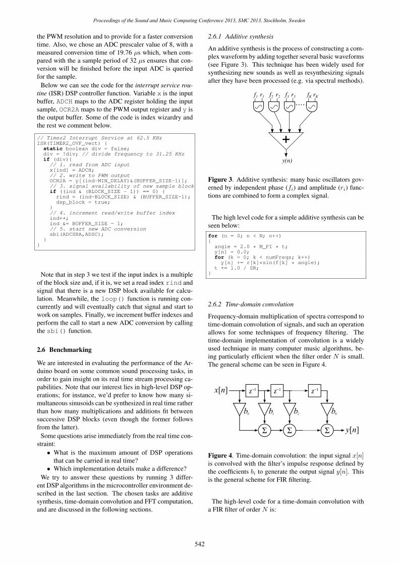
2.6.1 Additive synthesis

An additive synthesis is the process of constructing a com-plex waveform by adding together several basic waveforms(see Figure 3). This technique has been widely used forsynthesizing new sounds as well as resynthesizing signalsafter they have been processed (e.g. via spectral methods).

Figure 3. Additive synthesis: many basic oscillators gov-erned by independent phase (fi) and amplitude (ri) func-tions are combined to form a complex signal.

The high level code for a simple additive synthesis can beseen below:for (n = 0; n < N; n++){

angle = 2.0 * M_PI * t;y[n] = 0.0;for (k = 0; k < numFreqs; k++)

y[n] += r[k]*sin(f[k] * angle);t += 1.0 / SR;

}

2.6.2 Time-domain convolution

Frequency-domain multiplication of spectra correspond totime-domain convolution of signals, and such an operationallows for some techniques of frequency filtering. Thetime-domain implementation of convolution is a widelyused technique in many computer music algorithms, be-ing particularly efficient when the filter order N is small.The general scheme can be seen in Figure 4.

Figure 4. Time-domain convolution: the input signal x[n]is convolved with the filter’s impulse response defined bythe coefficients bi to generate the output signal y[n]. Thisis the general scheme for FIR filtering.

The high-level code for a time-domain convolution witha FIR filter of order N is:

542

Proceedings of the Sound and Music Computing Conference 2013, SMC 2013, Stockholm, Sweden

for (k = 0; k < N; k++)y[n] += b[k]*x[n-k];

2.6.3 Fast Fourier Transform

The Fast Fourier Transform (FFT) is a clever implemen-tation of the traditional Fourier Transform that brings itscomplexity down from O(n2) to O(n log(n)), where nis the number of time-domain digital samples or, equiva-lently, the number of frequency bins that describe the fre-quency spectrum of the signal after the Transform compu-tation [6]. The FFT algorithm takes advantage of redun-dancy and symmetry on intermediary steps of the calcula-tion and is used in many signal processing algorithms. Thegeneral scheme of the FFT can be seen in Figure 5.

Figure 5. The FFT uses a divide-and-conquer approachand saves intermediate results to accelerate the calcula-tion of a signal spectrum. The figure shows one step ofan 8-point FFT calculation and how the results map to fre-quency bins.

2.6.4 Benchmarking

Each of the algorithms mentioned in the last sections havedifferent computational costs in terms of number of integerand floating-point operations, and quantity/size of memoryreads and writes.

In the context of real time audio processing in Arduino,these algorithms bring natural questions regarding feasibil-ity of processing:

• Additive synthesis: what is the maximum number ofoscillators that can be used to compute a new wave-form in real time?

• Time-domain convolution: what is the maximum lengthof a filter that can be applied to an audio signal inreal time?

• FFT: what is the maximum length of an FFT that canbe computed in real time?

3. RESULTS

3.1 Additive synthesis

The first experiment tries to answer the question of howmany oscillators can be used when performing real time

additive synthesis inside the platform. In the beginning ofthe DSP cycle, an additive synthesis algorithm is run usinga determined number of oscillators and the mean of thesynth time is taken over ten million measurements. Blocksizes used had 32, 64 and 128 samples (more showed to beunfeasible in real time) and the number of oscillators wasincreased until the DSP cycle period was exceeded.

The first result has to do with the use of loop structures.Because looping usually requires incrementing and testinga variable in each iteration, the use of one loop structuremay have strong influence in the amount of oscillators thatcan be used in real time for additive synthesis inside theArduino.

In any DSP algorithm that works over a block of samplesthere is at least one loop structure, that loops over all sam-ples of the block. This loop could be eliminated at the costof having to recompile the code every time the length ofthe block is changed, which is highly inconvenient. Usu-ally more loops will be used, for instance in additive syn-thesis for summing the result of several oscillators. Weinvestigate the alternative of removing this inner loop, byexplicitly writing the sum of oscillators. Figure 6 showsthe maximum amount of oscillators feasible in real timeby making use of a loop and by making use of inline code.By removing the inner loop we were able to increase from8 oscillators to 13 or 14 depending on the block size.

0

1

2

3

4

5

0 1 2 3 4 5 6 7 8 9 10 11 12 13 14 15

Synth

tim

e (

ms)

Number of oscilators

Additive Synthesis on Arduino (using a loop)

0

1

2

3

4

5

0 1 2 3 4 5 6 7 8 9 10 11 12 13 14 15

Synth

tim

e (

ms)

Number of oscilators

Additive Synthesis on Arduino (using inline code)

bl. size 32rt per. 32

bl. size 64

rt per. 64bl. size 128rt per. 128

Figure 6. Additive synthesis results using loops (above)and inline code (below).

543

Proceedings of the Sound and Music Computing Conference 2013, SMC 2013, Stockholm, Sweden

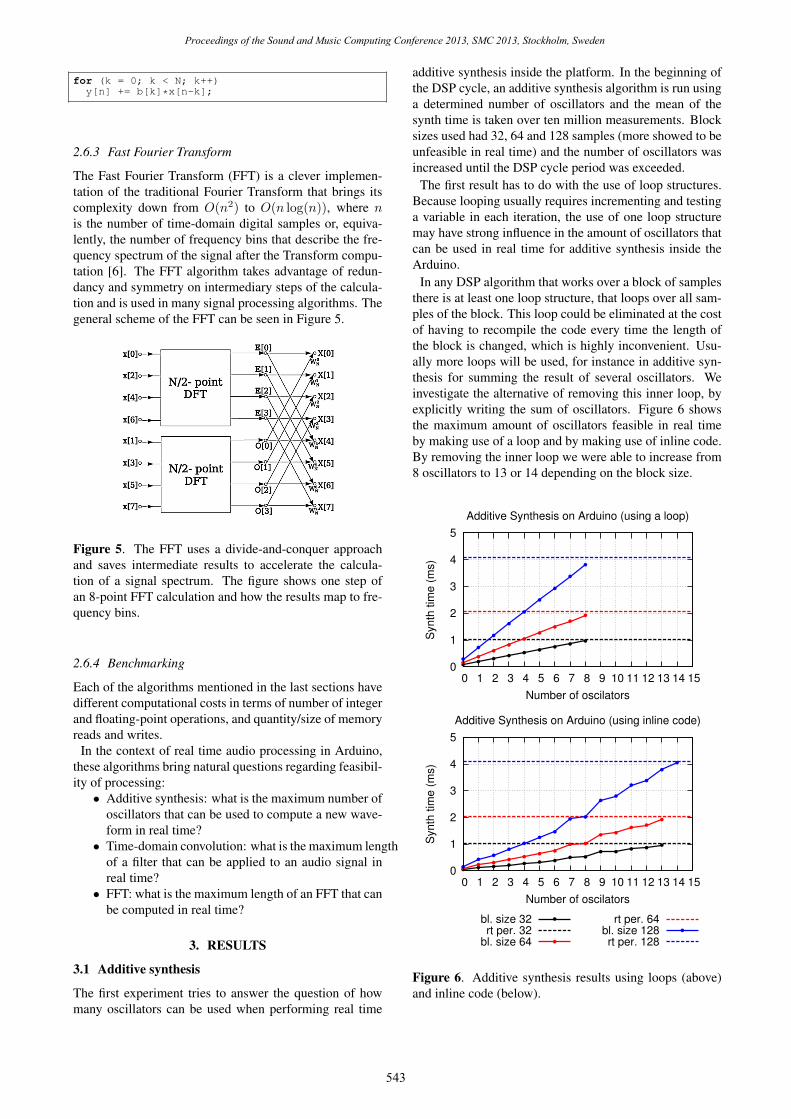
While implementing this experiment, a first attempt wasmade using the standard API sin() function. As thatproved to be unfeasible in real time, we focused on tablelookup implementations. At this point we noticed that eventhe smallest implementation difference can have large im-pact on the results. Therefore, we decided to test and plotthe results for slightly different implementations.

Two parameters are used to calculate the value of eachoscillator: phase and amplitude. Phase is handled by up-dating the index for sine table reads, and then the amplitudehas to be multiplied by the value obtained by the lookup.Floating point operations are also extremely expensive inthe platform we are using, so we implemented 3 differ-ent ways of multiplying the amplitude: (1) by using oneinteger multiplication and one integer division (2 integeroperations), (2) by using only one integer division (1 in-teger operation), and (3) by using variable bit padding forperforming bitwise power of 2 divisions or multiplications.Figure 7 shows the time used by the additive synthesis al-gorithm using these variants. By making use of lower leveloperations (that achieve less precise results) and inline cod-ing we were able to raise the number of oscillators from3 (when using 2 integer operations and a for loop) to 15(when using a variable pad and inline code).

0

1

2

3

4

5

0 1 2 3 4 5 6 7 8 9 10 11 12 13 14 15

Synth

tim

e (

ms)

Number of oscilators

Operations in additive synth (R=31250/N=128)

mult/divdiv

var padrt period

Figure 7. Time taken for additive synthesis algorithm withblock size of 128 samples, using different number andkinds of operations and variable number of oscillators.

3.2 Time-domain convolution

Our second experiment tries to clarify what is the maxi-mum size of a FIR filter that can be applied in real timeto an input signal by use of time-domain convolution algo-rithms. Following lessons learned on the first experiment,we implemented the filtering loop using different types ofoperations for multiplying each coefficient by the samplevalues: (1) using one integer multiplication and one integerdivision, (2) using variable pad, and (3) using a constanthardcoded pad. The results for each of these implemen-tations can be seen in Figure 8. This experiment was runwith a sample rate of 31250 Hz and block sizes of 32, 64,128 and 256 samples.

Results again show that small implementation differencesmake a big difference on computing power. When usinginteger division, the maximum order obtained for the filterwas 1, while by using a variable pad the order raised to 7and with constant padding we could achieve an order of 13or 14 depending on the block size.

0

1

2

3

4

5

6

7

8

9

0 1 2 3 4 5 6 7 8 9 10 11 12 13 14 15

Synth

tim

e (

ms)

Order of the filter

Time-domain convolution on Arduino (mult/div)

0

1

2

3

4

5

6

7

8

9

0 1 2 3 4 5 6 7 8 9 10 11 12 13 14 15

Synth

tim

e (

ms)

Order of the filter

Time-domain convolution on Arduino (variable pad)

0

1

2

3

4

5

6

7

8

9

0 1 2 3 4 5 6 7 8 9 10 11 12 13 14 15

Synth

tim

e (

ms)

Order of the filter

Time-domain convolution on Arduino (constant pad)

bl. size 32rt per. 32

bl. size 64rt per. 64

bl. size 128rt per. 128

bl. size 256rt per. 256

Figure 8. Time-domain convolution using 2 integer op-erations (top), variable padding (middle) and constantpadding (bottom).

3.3 FFT

The third experiment is concerned with the maximum lengthof an FFT that can be computed in real time inside an Ar-duino. In this case we chose to evaluate a standard imple-

544

Proceedings of the Sound and Music Computing Conference 2013, SMC 2013, Stockholm, Sweden

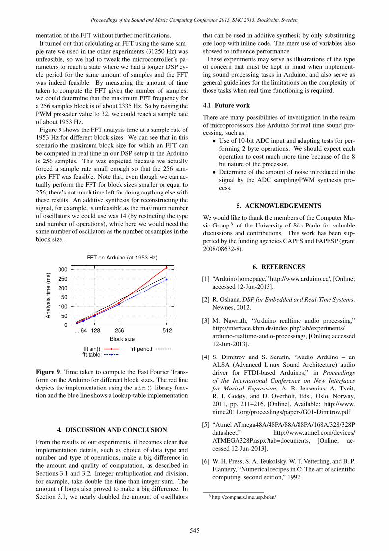
mentation of the FFT without further modifications.It turned out that calculating an FFT using the same sam-

ple rate we used in the other experiments (31250 Hz) wasunfeasible, so we had to tweak the microcontroller’s pa-rameters to reach a state where we had a longer DSP cy-cle period for the same amount of samples and the FFTwas indeed feasible. By measuring the amount of timetaken to compute the FFT given the number of samples,we could determine that the maximum FFT frequency fora 256 samples block is of about 2335 Hz. So by raising thePWM prescaler value to 32, we could reach a sample rateof about 1953 Hz.

Figure 9 shows the FFT analysis time at a sample rate of1953 Hz for different block sizes. We can see that in thisscenario the maximum block size for which an FFT canbe computed in real time in our DSP setup in the Arduinois 256 samples. This was expected because we actuallyforced a sample rate small enough so that the 256 sam-ples FFT was feasible. Note that, even though we can ac-tually perform the FFT for block sizes smaller or equal to256, there’s not much time left for doing anything else withthese results. An additive synthesis for reconstructing thesignal, for example, is unfeasible as the maximum numberof oscillators we could use was 14 (by restricting the typeand number of operations), while here we would need thesame number of oscillators as the number of samples in theblock size.

0

50

100

150

200

250

300

... 64 128 256 512

Analy

sis

tim

e (

ms)

Block size

FFT on Arduino (at 1953 Hz)

fft sin()fft table

rt period

Figure 9. Time taken to compute the Fast Fourier Trans-form on the Arduino for different block sizes. The red linedepicts the implementation using the sin() library func-tion and the blue line shows a lookup-table implementation

4. DISCUSSION AND CONCLUSION

From the results of our experiments, it becomes clear thatimplementation details, such as choice of data type andnumber and type of operations, make a big difference inthe amount and quality of computation, as described inSections 3.1 and 3.2. Integer multiplication and division,for example, take double the time than integer sum. Theamount of loops also proved to make a big difference. InSection 3.1, we nearly doubled the amount of oscillators

that can be used in additive synthesis by only substitutingone loop with inline code. The mere use of variables alsoshowed to influence performance.

These experiments may serve as illustrations of the typeof concern that must be kept in mind when implement-ing sound processing tasks in Arduino, and also serve asgeneral guidelines for the limitations on the complexity ofthose tasks when real time functioning is required.

4.1 Future work

There are many possibilities of investigation in the realmof microprocessors like Arduino for real time sound pro-cessing, such as:

• Use of 10-bit ADC input and adapting tests for per-forming 2 byte operations. We should expect eachoperation to cost much more time because of the 8bit nature of the processor.

• Determine of the amount of noise introduced in thesignal by the ADC sampling/PWM synthesis pro-cess.

5. ACKNOWLEDGEMENTS

We would like to thank the members of the Computer Mu-sic Group 6 of the University of Sao Paulo for valuablediscussions and contributions. This work has been sup-ported by the funding agencies CAPES and FAPESP (grant2008/08632-8).

6. REFERENCES

[1] “Arduino homepage,” http://www.arduino.cc/, [Online;accessed 12-Jun-2013].

[2] R. Oshana, DSP for Embedded and Real-Time Systems.Newnes, 2012.

[3] M. Nawrath, “Arduino realtime audio processing,”http://interface.khm.de/index.php/lab/experiments/arduino-realtime-audio-processing/, [Online; accessed12-Jun-2013].

[4] S. Dimitrov and S. Serafin, “Audio Arduino – anALSA (Advanced Linux Sound Architecture) audiodriver for FTDI-based Arduinos,” in Proceedingsof the International Conference on New Interfacesfor Musical Expression, A. R. Jensenius, A. Tveit,R. I. Godøy, and D. Overholt, Eds., Oslo, Norway,2011, pp. 211–216. [Online]. Available: http://www.nime2011.org/proceedings/papers/G01-Dimitrov.pdf

[5] “Atmel ATmega48A/48PA/88A/88PA/168A/328/328Pdatasheet,” http://www.atmel.com/devices/ATMEGA328P.aspx?tab=documents, [Online; ac-cessed 12-Jun-2013].

[6] W. H. Press, S. A. Teukolsky, W. T. Vetterling, and B. P.Flannery, “Numerical recipes in C: The art of scientificcomputing. second edition,” 1992.

6 http://compmus.ime.usp.br/en/

545

Proceedings of the Sound and Music Computing Conference 2013, SMC 2013, Stockholm, Sweden