1

MEE09:71

Real Time Automatic Step Detection in the three

dimensional Accelerometer Signal implemented on a Microcontroller System

Aylar Seyrafi

This thesis is presented as part of Degree of Master of Science in Electrical Engineering

Blekinge Institute of Technology December 2009

Blekinge Institute of Technology School of Engineering

Department of Applied Signal Processing Supervisor: Dr. Michael Schiek

Mikael Swartling Examiner: Dr. Jörgen Nordberg

2

3

Abstract

Parkinson’s disease is associated with reduced coordination between respiration and locomotion.

For the neurological rehabilitation research, it requires a long-time monitoring system, which

enables the online analysis of the patient’s vegetative locomotor coordination. In this work a real

time step detector using three-dimensional accelerometer signal for the patients with Parkinson‘s

disease is developed. This step detector is a complement for a recently developed system

included of intelligent, wirelessly communicating sensors. The system helps to focus on the

scientific questions whether this coordination may serve as a measure for the rehabilitation

progress of PD patients.

4

5

Acknowledgements

I would like to express my gratitude to all those who gave me the possibility to complete this

thesis. I want to thank The Central Institute for Electronics (ZEL) of research center of Jülich, to

do the necessary research work and to use the departmental data I am deeply indebted to my

supervisors Dr. Micheal Schiek and from the research center of Jülich (FZJ), Mikael Swartling

and my examiner Dr. Jorgen Nordberg from Blekinge Institute of Technology (BTH) whose help,

stimulating suggestions and encouragement helped me in all the time of research for and writing

of this thesis. I also want to thank my colleagues, Mr. Mario Schlösser and Mrs. Hong Ying for

all their help, support, interest and valuable hints.

Especially, I would like to give my special thanks to my dear family whose support and love

enabled me to complete this work.

6

Table of Contents

Chapter1: Introduction ............................................................................................................ 11 1.1 Parkinson’s disease ..................................................................................................................................11

1.1.1 What is Parkinson’s disease? ...........................................................................................................11 1.1.2 What causes Parkinson’s disease?....................................................................................................11

1.2 Locomotor respiratory coordination in PD patient .....................................................................................13 1.3 Outline of the Current Work .....................................................................................................................14

Chapter2: Distributed intelligent sensor network for neurological rehabilitation research........ 15 2.1 System design ..........................................................................................................................................16 2.2 Analogue Front-Ends ...............................................................................................................................17 2.3 DAQ and the Frame Based OS .................................................................................................................18 2.4 Wireless Network .....................................................................................................................................20 2.5 Time Synchronization ..............................................................................................................................20

Chapter3: Instruments for step detecting ................................................................................. 23 3.1 (Commercial) Instruments ........................................................................................................................23

3.1.1 Pedometer .......................................................................................................................................23 3.1.2 Accelerometer .................................................................................................................................24 3.1.3 Pressure Mat ...................................................................................................................................24 3.1.4 Gyroscope .......................................................................................................................................25 3.1.5 Conclusion ......................................................................................................................................25

3.2 Accelerometer Sensor...............................................................................................................................26 3.3 FSR Sensor ..............................................................................................................................................27

3.3.1 Signal Conditioning Circuit .............................................................................................................28 3.3.2 FSR Sensor Signals .........................................................................................................................30

Chapter4: Step detection algorithm based on accelerometer signals ........................................ 32 4.1 Theoretical Background of Methods for Processing 1D or 2D accelerometer signals .................................32

4.1.1 Pan-Tompkins Method ....................................................................................................................32 4.1.2 Template Matching Method.............................................................................................................33 4.1.3 Peak-detection method based on combined dual-axial signals ..........................................................34

4.2 Algorithm for 3D accelerometer data ........................................................................................................36 4.3 Developed algorithm for step detection .....................................................................................................38

4.3.1 Steps of processing the walking signals made by 3D accelerometers ................................................39 Chapter5: Evaluation of step detecting algorithm of 3D accelerometer signals ........................ 42

5.1 Evaluation of results achieved by GUI ......................................................................................................42 Chapter6: Online implementation of step detection algorithm ................................................. 46

Chapter7: Fixed Point Arithmetic ........................................................................................... 53 7.1 Fixed point numbers .................................................................................................................................53 7.2 Q-format ..................................................................................................................................................54 7.3 Numerical operation .................................................................................................................................54 7.4 Hardware multiplier .................................................................................................................................55 7.5 Precision Loss and Error...........................................................................................................................56

7.5.1 Truncation error ..............................................................................................................................56 7.5.2 Overflow ........................................................................................................................................57 7.5.3 Underflow .......................................................................................................................................57

7.6 Division ...................................................................................................................................................57 7.7 Defining appropriate data format: .............................................................................................................57

Chapter8: Conclusion and future work.................................................................................... 60 8.1 Perspectives .............................................................................................................................................61

7

Abbreviations…………………......................................................................................................63 Bibliography……………………………………………………………………………………...65 Appendix…….…………………………………………………………………………………...70

8

Table of Figures Figure1.1: Areas which neurons that degenerate in PD are located ............................................ 12

Figure 1.2: Typical phase histogram of locomotion over a respiration period of a healthy

(Gesund) subject and two PD patients (Parkinson-Patienten) [3] ................................................ 13

Figure 2.1: Main board configuration multi-sensor DAQ iNODE. The MSP430 core (center) is

connected via flex-PCB to external peripherals and communication interfaces e.g. CC2420 IEEE

802.15.4 compliant RF-transceiver (left), analog front-ends and amplifiers e.g. accelerometer

(right). When folded to a cube the dimensions are 20mm per rim and the iNODE weights less

than 15 g including the LiIon battery. ........................................................................................ 15

Figure 2.2: Conceptual design of iNODE system. ...................................................................... 16

Figure 2.3: Concept of an unfolded iNODE in flex-PCP design. This way the iNODE can

seamlessly be integrated into belt worn applications. ................................................................. 17

Figure 2.4: Compact cubed iNODE 20x20x20 mm for barn owl application. This cube can be

mounted unnoticeable on the owls head. .................................................................................... 17

Figure 2.5: Example for evoked single unit activity (midbrain) recorded with iNODE front-end

using a standard wolfram electrode. ........................................................................................... 18

Figure 2.6: DMA-based dataflow for lossless DAQ. A DMA transfer concept combined with

storage switching assures power optimized and lossless data acquisition from the ADC to SD

memory. .................................................................................................................................... 19

Figure 2.7: Free CPU resources with different sample- and CPU clock frequencies [4] .............. 19

Figure 2.8: Sequence diagram illustrating synchronization mechanism between PC and iNODE.

The Master device puts all iNODEs into “waiting for synchronization” before it broadcasts a

trigger beacon. All iNODEs change to working state synchronously. Within the frame duration

TFrame one designated iNODE sends a synch feedback with a delay of ΔT. Master starts Main

FrameTimer for each iNODE indicating its online status. For prioritized communication the

online state is subdivided into receive (RX) and transmit (TX) scopes [4]. ................................. 21

Figure 2.9: Arithmetic mean shows characteristics similar to a normal distribution bell curve. The

trigger pulse width of 800 ns results from internal processing reasons and needs to be subtracted

from total curve [4]. ................................................................................................................... 21

Figure 3.1: A digital Omron HJ-112 pedometer ......................................................................... 23

Figure 3.2: Mat Platform Pressure Measurement System ................................................... 24

Figure 3.3: A schematic of Gyroscope ................................................................................... 25

9

Figure 3.4: Schematic diagram of the accelerometer circuit. ............................................... 27

Figure 3.5: (a).A typical FSR sensor, (b).FSR placement underneath the foot ............................ 27

Figure 3.6: Diagram of a typical force sensing resistor ............................................................... 28

Figure 3.7: Schematic diagram of the signal conditioning circuit with FSR sensor. .................... 29

Figure 3.8: FSR voltage divider with analog low-pass filter. ...................................................... 29

Figure 3.9: Schematic circuit of comparator............................................................................... 30

Figure 3.10: The output signals of FSR voltage divider and comparator..................................... 31

Figure 4.1: Block diagram of the Pan-Tompkins algorithm. ....................................................... 32

Figure 4.2: Flowchart of template matching ............................................................................... 34

Figure 4.3: X- and z- axial output signals of the accelerometer on the left and right feet of PD

patient. ...................................................................................................................................... 35

Figure 4.4: Block diagram of the peak detection method based on the combined dual-axial signal.

.................................................................................................................................................. 36

Figure 4.5: Flow chart of gait detection algorithm. SD_X (Y, Z) means the standard deviation of

X (Y, Z) acceleration signal. ...................................................................................................... 37

Figure 4.6: Whole signals acquired from walking test. ‘L’ (‘R’) means left (right) leg.

Accelerations, foot pressure and video image could be compared synchronously [18]. .............. 37

Figure 4.7: Gait detection result. The thin box marked by ‘G’ is the automatically detected gait

[18]. .......................................................................................................................................... 38

Figure 4.8: 3D accelerometer attachment to both ankles: X, Y and Z are three axes of sensors

and equivalent to horizontal, vertical and transverse direction respectively. ............................... 39

Figure 4.9: The standard deviation of block of 1 second is depicted in light blue and the original

walking signal is illustrated in dark blue of X-axis of a healthy person. ..................................... 40

Figure 4.10: Swing-stance phase discrimination for step signals of a healthy person. ................. 41

Figure 5.1: An annotation using MATLAB GUIDE toolbox. Illustration of step signals and

standard deviation of each blocks signals of X-axes from both ankles in dark and light blue

respectively. .............................................................................................................................. 43

Figure 5.2: An annotation using MATLAB GUIDE toolbox. Illustration of step signals (dark

blue) and standard deviation of each blocks signals (light blue) and also swing phase signal of X-

axis from both ankles. ................................................................................................................ 43

Figure 5.3: An annotation using MATLAB GUIDE toolbox. Illustration of step signals (dark

blue), standard deviation of each blocks signals (light blue) and swing phase signals of X-axis

10

from both ankles and also signals from FSR sensors in green color are selected, which can be

compared with the acc. signals. .................................................................................................. 44

Figure 5.4: A zoomed in version of swing-stance discrimination’s result, in intervals that FSR

signals are not reliable for step detection.................................................................................... 45

Figure 6.1: Concept of online implementation of the algorithm .................................................. 47

Figure 6.2: Final graph of stop-moving discrimination ............................................................... 49

Figure 6.3: A schematic of searching for swing phase over a buffer length of two seconds. ....... 49

Figure 6.4: Final result of swing-stance discrimination .............................................................. 50

Figure 6.5: A schematic view of online implementation of step detection algorithm....................51 Figure 7.1: Some examples of numbers in two’s complement .................................................... 54

Figure 7.2: Some Q-7 binary numbers and their conversion to decimal numbers ........................ 54

11

Chapter1: Introduction The goal of this work is to develop a real time step detector using three-dimensional

accelerometer signal instead of force sensitive resistor (FSR) signals for the patients with

Parkinson’s disease (PD). This detector shall complement a recently developed system of

intelligent, wirelessly communicating sensors for long term recording the locomotor respiratory

coordination in PD patients. The system shall help to focus on the scientific questions whether

this coordination may serve as a measure for the rehabilitation progress of PD patients and

whether this progress may benefit from real time feedback based relearning of this coordination

provided by this system. The advantages expected from using accelerometer signal for step

detection are, first more convenient attachment procedure of the accelerometer and secondly the

obtainment of extra information concerning e.g. tremor and gait dynamics.

1.1 Parkinson’s disease In this section, Parkinson disease and its symptoms are discussed.

1.1.1 What is Parkinson’s disease? Parkinson’s disease is a progressive, neurodegenerative, movement disorder [1].

• Progressive: Parkinson’s disease gets worse over time.

• Neurodegenerative: Parkinson’s disease is caused by the degeneration of nerve cells in

the brain.

• Movement disorder: the most prominent symptoms of Parkinson’s disease affect

movement, although many other symptoms may also occur, some of which can be even

more disabling than the movement symptoms.

Movement symptoms of Parkinson’s disease include [1]:

• Tremor: trembling in the hands, arms, legs, jaw and face

• Rigidity: stiffness of the limbs and trunk

• Bradykinesia: slowness of movement

• Akinesia: difficulty in initiating movement

• Postural instability: impaired balance

1.1.2 What causes Parkinson’s disease? The neurons that degenerate in Parkinson’s disease are located in several areas of the brain, but

most significant is the loss of dopamine-producing neurons in the substantia nigra. The dopamine

12

produced by these neurons is crucial for another brain region, called the striatum (see Fig. 1.1).

Under the influence of dopamine, signals from the striatum regulate all forms of voluntary

movement. The loss of dopamine in Parkinson’s disease accounts for most of the movement-

related symptoms of the disease.

Figure1.1: Areas which neurons that degenerate in PD are located

Parkinson's disease is characterized by tremor when muscles are at rest (resting tremor),

increased muscle tone (rigidity), slowness of voluntary movements, and difficulty maintaining

balance (postural instability).

• Parkinson's disease results from degeneration in the part of the brain that helps coordinate

movements.

• Usually, the most obvious symptom is tremors that occur when muscles are relaxed.

• Muscles become stiff, movements become slow and uncoordinated, and balance is easily

lost.

Parkinson's disease affects about 1 of 250 people older than 40, about 1 of 100 people older than

65, and about 1 of 10 people older than 80. It commonly begins between the ages of 50 and 79.

Rarely, Parkinson's disease occurs in children or adolescents. In about two thirds of people,

tremors are the first symptom. In others, the first symptom is usually problems with movement or

a reduced sense of smell. Parkinson's disease typically causes the following symptoms:

• Tremors: Tremors are coarse and rhythmic. They usually occur in one hand while the

hand is at rest (a resting tremor). The tremor is called a pill-rolling tremor because the

hand moves as if it is rolling small objects around. The tremor decreases when the hand is

moving purposefully and disappears completely during sleep. Emotional stress or fatigue

may worsen the tremor. The tremor may eventually progress to the other hand, the arms,

13

and the legs. A tremor may also affect the jaws, tongue, forehead, and eyelids, but not the

voice. In some people, a tremor never develops.

• Stiffness (rigidity): Muscles become stiff, impairing movement. When the forearm is

bent back or straightened out by another person, the movement may feel stiff and ratchet-

like (called cogwheel rigidity).

• Slowed movements: Movements become slow and difficult to initiate, and people tend to

move less. Thus, mobility decreases.

• Difficulty maintaining balance and posture: Posture becomes stooped, and balance is

difficult to maintain, leading to a tendency to fall forward or backward. Because

movements are slow, people often cannot move their hands quickly enough to break a

fall.

Walking becomes difficult, especially taking the first step. While walking, some people have

difficulty stopping or turning. When the disease is advanced, some people suddenly stop walking

because they feel as if their feet are glued to the ground (called freezing). Other people

unintentionally and gradually quicken their steps, breaking into a stumbling run to avoid falling.

This symptom is called festination [1][2].

1.2 Locomotor respiratory coordination in PD patient Parkinson disease is correlated with reduced coordination between respiration and locomotion

[3]. Fig.1.2 illustrates a typical histogram of the step event, characterized by heel strike,

superimposed on a respiration period for a healthy subject and two PD patients [3].

Figure 1.2: Typical phase histogram of locomotion over a respiration period of a healthy (Gesund)

subject and two PD patients (Parkinson-Patienten) [3]

14

This histogram informs that the steps are harmonized with respiration in a healthy subject,

whereas in PD patients the distribution of the heel strike events in contrast to breath is more or

less splitting. This reduced coordination between locomotion and respiration would measure the

health status of the patients. For the neurological rehabilitation research, a long-term monitoring

system is required in order to achieve the online analysis of vegetative locomotion coordination

of the patients. This online monitoring and analyzing allows the later integration of bio-feedback

protocol for the rehabilitation purpose. Measuring the therapeutic effect and PD’s health status

are benefits of this system.

1.3 Outline of the Current Work The current work contains seven broad parts. In chapter 2, introduces the distributed intelligent

sensor network device for neurological rehabilitation research in details and explains about the

area which step detection algorithm has been used in this application. Chapter 3 is gone through

the different instruments for step detection and the advantages and also disadvantages of these

tools and pointing out to some reasons why specific devices should be used in this research. The

general background and previous and also new developed algorithms in details is explained in

chapter 4. In chapter 5 the results of offline implementation of developed algorithm has been

evaluated and the steps of online implementation and also its results is clarified in chapter 6.

Methods of converting from floating point to fixed point arithmetic and providing data for

implementing the whole algorithm into micro controller is covered by chapter 7.

15

Top View

Bottom View

Chapter2: Distributed intelligent sensor network for neurological rehabilitation research

For the neurological rehabilitation research application a multi channel, wireless networking Data

acquisition (DAQ), battery driven system for implementing real-time digital signal processing

and feedback experiments has been developed within the ZEL (CENTRAL INSTITUTE FOR

ELECTRONICS) of research center Jülich [4]. The iNODE (intelligent Network Operating

DEvice ) system is based on a Texas Instrument MSP430 micro-controller provides lossless local

data storage up to 16GB with outer dimensions of 20mm per rim and less than 4.5 gram plus a

lithium-Ion battery. This sensor node is able to record signals up to 8 channels with sample rate

of up to 8 KHz each and also affords adequate CPU power for digital signal processing and

arranged for the mobile experiment. An IEEE 802.15.4 (ZigBee) RF transceiver component

provides two ways communication between the sensor nodes. Wireless communication between

the sensor network and a PC for configuration purpose and online data visualization has been

implemented. To merge the lossless acquired data of the distributed iNODEs a time

synchronization protocol has been developed preserving causality which may offer new

opportunities in the treatment of neurological patients with real time analysis of these

synchronization processes and bio feedback capabilities [4].

Figure 2.1: Main board configuration multi-sensor DAQ iNODE. The MSP430 core (center) is

connected via flex-PCB to external peripherals and communication interfaces e.g. CC2420 IEEE 802.15.4 compliant RF-transceiver (left), analog front-ends and amplifiers e.g. accelerometer (right).

When folded to a cube the dimensions are 20mm per rim and the iNODE weights less than 15 g including the LiIon battery.

In the areas of neurological rehabilitation and sleep research the simple and comfortable long

term registration of vegetative and locomotor rhythm coordination is a challenging task. In this

project a miniaturized autonomous sensor node (iNODE, intelligent Network Operating DEvice)

is designed which includes a MSP430 microcontroller from Texas Instruments with internal and

16

external peripheral devices for further digital signal processing as well as digital controlled

analogue electronics for signal conditioning and pre-processing. For data-fusion of multiple

iNODEs a time synchronization protocol based on the Reference Broadcast Synchronization

(RBS) has been developed to preserve causality. In subsequent levels of development several

iNODEs will form a self configuring and self organizing network with modular design to keep it

open for multi-sensor data-acquisition and actuators. In Fig. 2.2, conceptual design of iNODE

system is illustrated.

Figure 2.2: Conceptual design of iNODE system.

2.1 System design The central component of the system is the Ultra-Low-Power microcontroller (µC) MSP430 with

a 16 Bit RISC CPU. The applied derivative F1611 includes considerably internal peripheral

components such as e.g. 10 kB static RAM, 48 kB Flash Memory, 12 Bit ADC with 8 Channels,

3 Channel DMA, 2 USART communication modules with SPI, I2C and UART. Presently the

CPU can be driven with up to 8 MHz [3]. The µC is connected via the SPI interface to a mass

storage device (SanDisk iNAND), which actually contains up to 4 GB memory capacity. This

device is compatible with the Secure Digital Card (SD flash memory) standard and features with

PCB dimensions and low power consumption in comparisons with other memory concepts. The

17

incoming analog signal is transformed according to the application and the ADC voltage range by

digital controlled analog pre-processing electronics. Acquired data will be losslessly stored in the

SD-flash memory and on demand be processed in the memory of the µC. Using an additional

adaptive power management the adjustment of driving CPU voltage concerning the chosen CPU-

clock frequency is achieved. The power consumption of the CPU is 330 µA @ 1 MIPS and 1.1

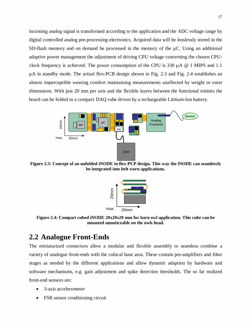
µA in standby mode. The actual flex-PCB design shown in Fig. 2.3 and Fig. 2.4 establishes an

almost imperceptible wearing comfort maintaining measurements unaffected by weight or outer

dimensions. With just 20 mm per axis and the flexible layers between the functional entities the

board can be folded to a compact DAQ cube driven by a rechargeable Lithium-Ion battery.

Sensor

LiIon

20m

m

20mmmax.

µCRF

AnalogFrontend

sw

Figure 2.3: Concept of an unfolded iNODE in flex-PCP design. This way the iNODE can seamlessly

be integrated into belt worn applications.

20m

m

20mmmax. Figure 2.4: Compact cubed iNODE 20x20x20 mm for barn owl application. This cube can be

mounted unnoticeable on the owls head.

2.2 Analogue Front-Ends The miniaturized connectors allow a modular and flexible assembly to seamless combine a

variety of analogue front-ends with the cubical base area. These contain pre-amplifiers and filter

stages as needed by the different applications and allow dynamic adaption by hardware and

software mechanisms, e.g. gain adjustment and spike detection thresholds. The so far realized

front-end sensors are:

• 3-axis accelerometer

• FSR sensor conditioning circuit

18

• Respiration amplifier to fit with SleepSences’© inductive belt

• ECG and EMG amplifier

• Amplifier for extra cellular single neuron recordings

An example of a stable recording of midbrain neuronal activity recorded in an anaesthetized Barn

Owl using the iNODE amplifier is shown in 2.5.

Figure 2.5: Example for evoked single unit activity (midbrain) recorded with iNODE front-end

using a standard wolfram electrode.

2.3 DAQ and the Frame Based OS The cyclic repetition of the DMA based DAQ sequence lined out in the following description

guarantees a continuously lossless data acquisition [5] and is the basis for our µC operating

system that takes advantage of a round-robin like scheduler concept called Frame Based

Operating System (FRABOS). The basic idea of this concept is a DMA switching mechanism for

data frames of 256 samples as shown in Fig 2.6. After the ADC sample and hold procedure a

digital value is stored in an internal register of the ADC. This triggers the DMA channel 0 to

transfer this value into the internal RAM of the µC. For this reason a memory block is allocated

as a double buffer where each buffer can catch 256 Samples with 16 Bit. This matches the block

size of the SD flash memory of 512 Bytes. Once one buffer is filled, the DMA triggers an

interrupt service routine (ISR) which directs the incoming dataflow to the second buffer.

Additionally the data transfer from the previous buffer to the SD flash memory will be initialised

and started by configuring the DMA channel 1 and linking it to the SPI interface.

19

Figure 2.6: DMA-based dataflow for lossless DAQ. A DMA transfer concept combined with storage

switching assures power optimized and lossless data acquisition from the ADC to SD memory.

Test measurements with a sampling frequency of 96 kHz for single channel DAQ have been

performed with the CPU clock frequency and the driving clock frequency of the SPI Module set

to 8 MHz. Using this configuration causes achieving free CPU resources of approximately 80%

as shown in Fig. 2.7.

Figure 2.7: Free CPU resources with different sample- and CPU clock frequencies [4]

20

2.4 Wireless Network Also integrated into this DAQ platform is the true single-chip 2.4 GHz IEEE 802.15.4 compliant

RF-Transceiver CC2420 from Chipcon to complement the node to a body sensor network with 10

m range and a maximum data rate of 250 kbit/s [6]. Based on the IEEE 802.15.4 wireless

standard a compact communication protocol with Reduced Function Device (RFD) capabilities

including association, data exchange and synchronization condensed to the so called “Ultra-

Small-Stack” (USS) was implemented to run on the ultra low power microcontroller platform.

Embedded into FRABOS this protocol already allows bidirectional communication between each

sensor node and a PC within a star topology. The extension to mesh topology communication is

under development. Both the USS and FRABOS were coded in embedded object oriented C++

achieving an adjustable mapping of hardware components to software objects and to provide a

functional encapsulation of the external peripherals. The assembled code on the MSP430

demands less than 25 kB total of the available 48 kB flash without optimization. The round-robin

scheduler FRABOS itself requests less than 20 kB and the Ultra-Small-Stack for RF less than 7

kB to achieve a net data rate of 141 kbit/s thus creating an avenue for wireless live-streaming 8

kHz measurements with up to 16 Bit accuracy and provides enormous potential for future bio

medical and neurophysiological applications. For a multi-vendor convertible wireless PC

connection a ZigBee compliant and IEEE 802.15.4 compatible USB dongle from Integration

Associates OEM-DAUB1 2400 is used. To enable comfortable configuration access to the

iNODE parameters, to give access to the recorded data on the SD-Card and to administrate the

wireless network with a PC using RS232 or RF interface we developed a Graphical User

Interface. The GUI also gives opportunities to plot and filter downloaded or life-stream data by

using the cross-platform framework Qt4 for development.

2.5 Time Synchronization For the time synchronous data acquisition of multiple iNODEs the Reference Broadcast

Synchronization (RBS) has been adopted and modified [7]. Besides the synchronous start of the

measurement for all associated iNODEs the implemented protocol also assures the

communication within specific time windows Fig. 2.8. This way the power management is

capable of an adaptive control of the iNODE’s duty cycle by managing the CC2420 online and

offline status.

21

SlaveSlaveMasterMaster

WaitSyncRequest

Beacon

SyncResponse ∆T

TimerMFTTimerMFT TimerOnTimerOn OnlineOnline WorkingWorking IdleIdleGUIGUI

timeout changeTo_Idle

timeout

Idle

timeout

isOnline

isOnline

ACK

RX

TX

killTimer

Shutdown

Idle

t

Figure 2.8: Sequence diagram illustrating synchronization mechanism between PC and iNODE. The

Master device puts all iNODEs into “waiting for synchronization” before it broadcasts a trigger beacon. All iNODEs change to working state synchronously. Within the frame duration TFrame one designated iNODE sends a synch feedback with a delay of ΔT. Master starts Main FrameTimer for

each iNODE indicating its online status. For prioritized communication the online state is subdivided into receive (RX) and transmit (TX) scopes [4].

The analysis of the jitter indicated by the span of time variation between synchronization signal

and starting of the data acquisition was analysed with 512 single measurements.

tenv = 3,78µs

∆tpulse = 800ns

Figure 2.9: Arithmetic mean shows characteristics similar to a normal distribution bell curve. The trigger pulse width of 800 ns results from internal processing reasons and needs to be subtracted

from total curve [4].

The results show that the protocol ensures a synchronous start of measurement and a frame based

duty cycle adjustment with an appropriate precision proven by a jitter of about ±1.47 µs. Due to a

22

specification caused debug-pulse width of 800 ns the averaged measurement in Fig 2.9 needs to

be interpreted correctly. The implemented Ultra Small Stack communication protocol creates an

avenue for live-streaming 8 kHz measurements with up to 16 Bit accuracy. The duration of 62.5

µs for one sample considering the measured jitter determines an error ratio of 2.35 % and is

evanescent for human application with sample rates with 1 kHz.

23

Chapter3: Instruments for step detecting The system is aimed to be used for detecting the steps on both feet. In section 3.1, a variety of

tools which may be used for this purpose is presented. Then a summary of accelerometer

techniques is mentioned in section 3.2. After that Force Sensing Resistor (FSR) sensors which

mostly have been used as a standard of step detection, are introduced in section 3.3.At the end a

summary of this chapter is provided in section 3.4.

3.1 (Commercial) Instruments There are many different techniques available for assessment of human movement in the clinic,

laboratory and home. Detection of the gait events is primarily carried out by these tools:

pedometer, accelerometers, plantar pressure measurement system and gyroscope.

3.1.1 Pedometer A pedometer or step counter is a portable and electronic or electromechanical device about the

size of a pager that is capable of recording ambulatory activity such as walking, jogging, or

running. It will not count steps during activities such as cycling, rowing, upper body exercise, etc.

The accuracy of step counters varies widely between devices and also depends on the step-length

that user enters. Best pedometers are accurate to within ± 5% error [5]. The technology for a

pedometer includes a mechanical sensor and software to count steps. Today advanced step

counters rely on MEMS inertial sensors and sophisticated software to detect steps. These MEMS

sensors have either 1-, 2- or 3-axis detection of acceleration. The use of MEMS inertial sensors

permits more accurate detection of steps and fewer false positives. Pedometers typically range in

cost from $10-$50 depending on the features [6][7]. A digital pedometer is shown in figure 3.1.

Figure 3.1: A digital Omron HJ-112 pedometer

24

3.1.2 Accelerometer An accelerometer is an electromechanical device that will measure acceleration forces. These

forces may be static, like the constant force of gravity pulling at your feet, or they could be

dynamic - caused by moving or vibrating the accelerometer. Accelerometers known as

lightweight, inexpensive and low-power devices, provide quantitative measures of gait, they are

capable of identifying specific gait changes in older adults and can be used to objectively

quantify ambulatory activity levels. Accelerometers have many potential uses in monitoring of

patients in rehabilitation [8].

3.1.3 Pressure Mat Pressure Mat is a system for sensing and displaying the distribution of contact pressure caused by

a person's weight on a walkway. The system includes a flexible, pressure-sensitive mat,

electronics to activate the mat. Pressure Mat is a stand-alone device measuring vertical force and

pressure distribution. It can be used in conjunction with a force plate. The system provides

pressure and force information which is extremely helpful for evaluation and treatment of

children or deformed feet. A USB connection with new VersaTek electronics makes gait analysis

and foot function easier. Easy to use Windows® based software allows you to view real-time

dynamic weight transfer and local pressure concentrations, as well as capture multiple footstrikes

in seconds. The sensitivity of the sensor is adjustable and the sensor can be calibrated to convert

output into pressure units. Pressure mats can be provided for different applications such as in-

shoe, grip, prosthetic and seating. A pressure measurement’s platform is depicted in figure 3.2.

Figure 3.2: Mat Platform Pressure Measurement System

25

3.1.4 Gyroscope As it is shown in figure 3.3 a gyroscope is a device for measuring or maintaining orientation,

based on the principles of angular momentum. Using gyroscope is an alternative skill for step

detection. These sensors are able to attach anywhere to a body segment since the angular rotation

is still the same along the segment [9].

Figure 3.3: A schematic of Gyroscope

3.1.5 Conclusion In summary, the goal of this work is to determine the close timing of details of events during the

walking cycle in order to analyze the steps, but, pedometers just are able to count the steps while

walking which is not in the right direction of this work’s goal. However, plantar pressure can

give an accurate pressure distribution, but, the device which involved for measurement is too

large and the measured area too limited for measuring locomotion such as wide range steps or

running. So, these products obtain a variety of information but are too costly and complex for

practical use such as in rehabilitation [10]. Gyroscopes are extensively applied for step detection.

However, gyroscopes bring constant signal as accelerometers in term of heel-off and -strike

events detection [11]. Accelerometers mostly used for monitoring the step signal which caused a

wide usage of them. Due to the universal acceptance about the accuracy of FSR sensors in the

field of step detecting, accelerometers and FSR sensors both were further researched in the

following sections.

26

3.2 Accelerometer Sensor Observational techniques are an elemental part of step detection and as discussed accelerometers

can provide a useful objective adjunct. Many of the other techniques have significant

disadvantages for continuous analysis. Accelerometers need to be placed on the surface of the

object in order to determine the accurate vibrations. It must be firmly attached to the object in

order to give precise signals. For detecting the steps, a 3-axis accelerometer named ADXL330

which is a small, low-power consumption (less than 200 micro amps at 2.0 V) accelerometer with

signal conditioned voltage outputs all in a single monolithic IC, produced by Analogue Devices,

Inc., is used for determining the horizontal, vertical and transverse acceleration in x- and y- and

z-axis achieved from foot movement. ADXL330 measures acceleration with a minimum full-

scale range of ±2g. The output signals are analog voltages that are proportional to acceleration. It

can measure the static acceleration of gravity in tilt-sensing applications, as well as dynamic

acceleration resulting from motion, shock, or vibration. It contains a polysilicon surface

micromachined sensor and signal conditioning circuitry to implement an open-loop acceleration

measurement architecture. The sensor is a polysilicon surface micro machined structure built on

top of a silicon wafer. Polysilicon springs suspend the structure over the surface of the wafer and

provide a resistance against acceleration forces. Deflection of the structure is measured using a

differential capacitor that consists of independent fixed plates and plates attached to the moving

mass. The fixed plates are driven by 180° out-of-phase square waves. Acceleration deflects the

moving mass and unbalances the differential capacitor resulting in a sensor output whose

amplitude is proportional to acceleration. Phase-sensitive demodulation techniques are then used

to determine the magnitude and direction of the acceleration.

The demodulator output is amplified and brought off-chip through a 32 kΩ resistor. The user then

sets the signal band-width of the device by adding a capacitor. This filtering improves

measurement resolution and helps prevent aliasing. In Fig. 3.4 a schematic diagram of the

accelerometer circuit is illustrated.

27

Figure 3.4: Schematic diagram of the accelerometer circuit.

3.3 FSR Sensor Force Sensing Resistors (FSR) are a polymer film device, which exhibits a decrease in resistance

with an increase in the force or pressure applied to the active surface. Its force sensitivity is

optimized for use in human touch control of electronic devices.

(a) (b)

Figure 3.5: (a).A typical FSR sensor, (b).FSR placement underneath the foot Fig. 3.5(a) depicts a typical FSR sensor with a view of its dimension and in Fig. 3.5(b) the

placement of sensor underneath the foot for step detecting is indicated. A force sensing resistor is

made up of two parts. The first is a resistive material applied to a film.

28

Figure 3.6: Diagram of a typical force sensing resistor

The second is a set of digitizing contacts applied to another film. Fig. 3.6 shows this

configuration. The resistive material serves to make an electrical path between the two sets of

conductors on the other film. When a force is applied to this sensor, a better connection is made

between the contacts, hence the conductivity is increased. Over a wide range of forces, it turns

out that the conductivity is approximately a linear function of force (R

FCF 1, αα , where F is

force, C stands for capacitor and R for resistance). It is important to make note of the fact that

FSRs are not appropriate for accurate measurements of force due to the fact that parts might

exhibit as much as 15% to 25% variation between each other. The interface circuit of FSR sensor

in details is described in the section 3.3.1. And results of the FSR sensor circuit are stated in

section 3.3.2. [12]

3.3.1 Signal Conditioning Circuit An ideal electrical circuit is designed for step detection event which is included of heel-off phase

and heel-strike phase. Fig. 3.7 depicts the main elements of the signal conditioning circuit for

FSR sensor which is expressed by voltage regulator, FSR voltage divider, analogue low-pass

filter and comparator. To supply the signal conditioning circuit with 2.7 V voltage level by

battery, a low drop out voltage regulator TPS77027 by Texas instrument is applied. For detecting

the steps, the voltage divider circuit is designed to display a switch-like diagnostic based on FSR,

depicted in Fig. 3.8. The alternative amplifier OP281 is used in this circuit, ultra-low power, rail-

to-rail output operational amplifier produced by Analogue Device Inc.. This single-supply op-

29

amp is optimal for designing the miniaturized and battery-powered circuit. OP281 combines two

op-amps per chip.

Figure 3.7: Schematic diagram of the signal conditioning circuit with FSR sensor.

The first one is used in FSR voltage divider for negative feedback configuration, and the second

one is used in comparator for positive feedback configuration. Depend on negative feedback, the

output of op-amp in the FSR voltage divider is given as:

SOut VV = ×

I

FSR

RR

+1

1 (3.1)

where SV is the output of voltage regulator, which maintains 2.7 V. FSRR is the resistance of FSR

sensor, which ranges from 2 kΩ (maximal force applies on the sensor), to infinity (no force

applies to the sensor). A low-pass filter with cut-off frequency of 50 Hz behind the voltage

divider reduces the output signal, which consists of 2R and 3C in the Fig. 3.8.

Figure 3.8: FSR voltage divider with analog low-pass filter.

30

The output of low-pass filter is fed into a comparator with non-inverting input (see Fig. 3.9),

which converts the input signal into square wave. fVRe is determined by two resistor voltage

divider and 4R , 5R which is specified as:

fVRe = SV54

5

RRR+

× =1.08V (3.2)

Figure 3.9: Schematic circuit of comparator

To get rid of fluctuations in comparator circuits due to the noise, hysteresis is assigned by feeding

back to the positive input of op-amp which is a small fraction of the output voltage. This

basically means that there are two thresholds: +ThV and −ThV : [13]

VRR

VR

RRVV OMinfTh 3.1

6

3

6

63Re =×−

+×=+ (3.3)

VRR

VR

RRVV OMaxfTh 76.0

6

3

6

63Re =×−

+×=− (3.4)

To get the maximal positive output state OMaxV = 2.7 V, the input must rise above the threshold:

INU > +ThV , and to get the minimal output state OMinV = 0 V, the input must fall below the

threshold: INU < −ThV .

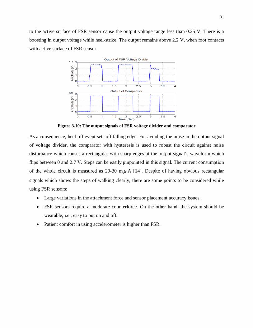
3.3.2 FSR Sensor Signals Fig. 3.10 illustrates the output signal of FSR voltage divider and comparator which is placed

underneath the foot of a healthy subject walking on the ground without encumbrance. As

exhibited on the output signal, there is a steep rising edge while foot strikes the ground and a

falling edge when foot rises off the ground. In case that foot lifts off the ground, no force assigns

31

to the active surface of FSR sensor cause the output voltage range less than 0.25 V. There is a

boosting in output voltage while heel-strike. The output remains above 2.2 V, when foot contacts

with active surface of FSR sensor.

Figure 3.10: The output signals of FSR voltage divider and comparator

As a consequence, heel-off event sets off falling edge. For avoiding the noise in the output signal

of voltage divider, the comparator with hysteresis is used to robust the circuit against noise

disturbance which causes a rectangular with sharp edges at the output signal’s waveform which

flips between 0 and 2.7 V. Steps can be easily pinpointed in this signal. The current consumption

of the whole circuit is measured as 20-30 mµ A [14]. Despite of having obvious rectangular

signals which shows the steps of walking clearly, there are some points to be considered while

using FSR sensors:

• Large variations in the attachment force and sensor placement accuracy issues.

• FSR sensors require a moderate counterforce. On the other hand, the system should be

wearable, i.e., easy to put on and off.

• Patient comfort in using accelerometer is higher than FSR.

32

Chapter4: Step detection algorithm based on accelerometer signals

Chapter 4 is going through the method for step detection based on 1D, 2D and 3D accelerometer

signals of the ankles. There are some methods which are previously developed [14]. In order to

provide the walking signals, two-dimensional accelerometer sensors are used for these methods

which are explained in detail through the section 4.1. Section 4.2 summarizes a gait detection

method which was the inspiration for developing the new algorithm that is described in section

4.3.

4.1 Theoretical Background of Methods for Processing 1D or 2D accelerometer signals

Previously an effort has been done to design a fast and robust algorithm, which should be suitable

for individual patients, without any user-specified parameters. Three methods have been

investigated for step detection in the accelerometer signals [14]:

• Pan-Tompkins method

• template-matching method

• peak-detection method based on combined dual-axial signals

The following subsections explain the theoretical backgrounds of these three methods. These

algorithm operates with the data recorded at the sample rate of 200 Hz, which meets the required

resolution 15 ms and sampling theorem. The entire spectral content of the original accelerometer

signal resides in the band of interest between 0 and 20 Hz.

4.1.1 Pan-Tompkins Method Pan and Tompkins [15][16], proposed a real-time algorithm for detection of some peaks in

electrocardiography (ECG) signal. Fig. 4.1 presents the entire procedures of the algorithm in

schematic form. This algorithm is modified to detect the steps in the accelerometer signal.

Figure 4.1: Block diagram of the Pan-Tompkins algorithm.

Band pass-filter: The band pass filter reduces the influence of artifacts in the signal. Because of

an analog high pass filter implemented in the signal conditioning circuit, only digital low pass

33

filters with a cutoff frequency of 20 Hz is applied. The digital low pass filters with small integers

are designed for fast execution, specified as:

21

24

)1()1(

161)( −

−

−−

=zzzH (4.1)

Derivative operator: The derivative operator suppresses the low-frequency components and

enlarges the high frequency components from the high slopes. An ideal derivative operator up to

30 Hz is approximated by:

)]4(2)3()1()(2[81)( −−−−−+= nxnxnxnxny (4.2)

Squaring: The squaring operation y(n) = [x(n)] 2 leads to positive results and enhances large

values more than small values.

Integration: The output of the derivative based operation will exhibit multiple peaks within a

single step cycle. The Pan-Tompkins algorithm performs smoothing of the output of the

preceding operations through a moving-window integration filter as:

)](...)2()1([1)( nxNnxNnxN

ny +++−++−= (4.3)

where N is chosen to be 20 empirically.

Fiducial mark: The so-called fiducial point, which is defined as location of the peak, is detected

using an adaptive threshold within the Pan-Tompkins method.

4.1.2 Template Matching Method The main concept of template-matching method is to generate a template, which represents a

typical step cycle. In the unknown signal, an event is declared to be detected when there is a

match between the signal and the template in certain degree. Fig. 4.2 illustrates the sequences of

peak detection using template matching method [14].

Initially, the whole recording is broken into several non-overlapping data blocks of 10 seconds

each. A template is generated by averaging the steps in the first data block of the recording

dataset. Then the current signal segment is filtered by a lowpass filter with cutoff frequency of 20

Hz. Next, the template is slid across the whole filtered data block and the normalized cross-

correlation is calculated between the template and the signal segment. The normalized cross-

correlation indicates the similarity between two vectors X and Y , which is defined as [17]:

][kRNorm =]0[]0[

][,

XYXY

XY

RRkR

YX

YX=

⋅

>< (4.4)

34

where X

is the norm of the vector X , ][kRXY is cross-correlation of X and Y for arbitrary k ,

and ]0[XXR is autocorrelation of ][nX at the point 0=k . The bound value for the maximum is 1

indicating the absolute identity, which allows setting an uniform threshold for all the data blocks

despite different amplitude. Thus a threshold of 0.4 is set to predict the occurrence of the step

event. The interval, in which the cross-correlation exceeds the threshold 0.4, is defined as peak-

searching interval. The local maxima falling within the peak-searching interval in the filtered

signal are marked as fiducial points of the steps. The morphology of the steps may change

dynamically with time. Thus the temporal template needs to be updated considering the current

data block in time. The result of the normalized cross-correlation, which indicates the similarity

between the template and the signal segment, determines whether a new template should be

computed. If great dissimilarity presents, the template will be updated by averaging the steps in

the current data block [14].

Figure 4.2: Flowchart of template matching

4.1.3 Peak-detection method based on combined dual-axial signals The third method is based on the coincident negative wave in the x- and z-axial acceleration

signal. Observe from Fig. 4.3 show that the negative wave in the x-axial signal occurs coincident

35

with the negative wave in the z-axial signal during each cycle. The negative peak due to the

deceleration before strike hitting the ground is higher than the positive peak. The process of this

algorithm follows steps illustrated in Fig. 4.4. At first, both signals, x- and z-axial acceleration,

pass through a lowpass filter with cutoff frequency of 20 Hz. Then the positive elements in both

arrays are set to zero, whereas the negative elements remain. Both arrays are summed up entry-

by-entry. Next, the intermediate results are smoothed using the moving-window integration filter.

Figure 4.3: X- and z- axial output signals of the accelerometer on the left and right feet of PD

patient.

Based on the slope wave, search interval is defined with a threshold, which is set as one fourth of

the maximum in array of the preprocessed signal. The index, whose value precedes the threshold

level, is identified as onset of the peak-searching interval. And width of the peak-searching

interval is equal to twice of the interval, whose values exceed the threshold. Local maxima falling

within the peak-searching interval in the filtered signal are marked as fiducial points of the step

[14].

36

Figure 4.4: Block diagram of the peak detection method based on the combined dual-axial signal.

4.2 Algorithm for 3D accelerometer data The developed algorithm which is revealed in details through the next section, has been inspired

by a study on a gait detection algorithm from 3 dimensional acceleration signals of ankles for the

patients with Parkinson’s disease by Jonghee Han, et al. [18]. In this section, a summery of this

paper is explained.

A general algorithm of gait detection with 3D acceleration signals of both ankles is presented.

Also a wearable activity monitoring system (W-AMS) has been used for monitoring the

accelerations. The foot pressure (Fedar-X) and the mentioned monitoring system were recorded

at the same time to be used as a reference of gait detection. This procedure consists of a control

board (which is included of, microcontroller, flash memory, RS232 module) and two sensor

modules (each consists of two dual-axis accelerometers placed on both ankles). There are some

steps followed by this automatic gait detection algorithm for processing the gait signals. At first

moving and stopping segment is distinguished by dividing the gait signal into the blocks of 1

second, by comparing the standard deviation of each block with the threshold stT (51 times the

standard deviation of gait signal). In case that this value is greater than the threshold stT , this

block will be counted as moving segment, else as a stopping segment. Same procedure is done

with moving blocks of 0.1 second (by dividing each moving block into 10 sub-blocks), in greater

than threshold stT case, the block will be counted as swing phase, else stance phase. After

achieving the swing phase, a simple peak search will be done on swing phase, among all the

clarified peaks, peaks which are found in vertical and horizontal acceleration signal

simultaneously were selected. In the selected peaks, peaks with amplitude higher than threshold

stT or peaks that the shape of the X and Y acceleration around them are almost the same will be

remained and other peaks will be deleted. Among the remained peaks if the interval of two

consecutive peaks is less than 0.5 second, one of them will be removed selectively. At last, the

37

remaining peaks are the gait peaks [19]. For automatic gait detection algorithm, the gait signal

was processed sequentially depicted in Fig. 4.5.

Figure 4.5: Flow chart of gait detection algorithm. SD_X (Y, Z) means the standard deviation of X

(Y, Z) acceleration signal. Foot pressure, three dimensional accelerations of ankles and video recorded images which were

acquired simultaneously is illustrated in Fig. 4.6 and 4.7. All the signals were exactly

synchronized and could be compared easily.

Figure 4.6: Whole signals acquired from walking test. ‘L’ (‘R’) means left (right) leg. Accelerations, foot pressure and video image could be compared synchronously [18].

38

Figure 4.7: Gait detection result. The thin box marked by ‘G’ is the automatically detected gait [18].

4.3 Developed algorithm for step detection Previous methods which were developed for step detecting that were using FSR sensors and 2

dimensional accelerometer signals given the good results, but, as mentioned in section 3.2 and

3.3, there are some shortages using FSR and even the 2D accelerometer.

However, while using 2D accelerometer, signals are more accurate in recording locomotion

signals than FSR sensors, but, should not be forgotten that, 2D accelerometers are not able to

cover all directions, therefore some movements will be missing while recording. It has to be kept

in mind that the signal’s coordinate system is moving with the legs. Since the leg movement is

not restricted to a perfect vertical plane a transformation of the data to the static coordinate

system of the physical space is not feasible using this 2D data. In this case, 3D accelerometer can

cover this deficit and give more accurate signals with taking care of three dimensional

movements and tremor so, it is superior to 2D accelerometer. Some types of accelerometers can

be used to measure tilt as well as body movement. For this measurement, four patients suffering

from PD and three healthy people were measured in the Center for Sleep and Rehabilitation

Research, Hagen-Ambrock,Germany under supervision of Prof. Schläfke, Dr. Schäfer. All were

walking around 8-10 minutes on the treadmill, with 3D accelerometer attached to the both ankle

39

according to the Fig. 4.8. The three axes of the sensors, X, Y and Z, correspond to horizontal,

vertical, and transverse direction (in respect to the coordinate system of the sensor) respectively.

Concurrently, FSR sensors are also attached underneath the foot in order to have a signal as a

reference with accurate swing and stance phase characterized by toe off and heel strike

respectively. In total, the dataset including of 8 channels, X-, Y-, Z-axis and FSR sensor for left

and also the same for the right foot, in duration of 70 minutes is collected from seven objects at a

sample rate of 512 Hz. Alternatively: Within all datasets the locomotion, i.e. walking, is always

present. Typically, in the X-axis, there is a smooth positive peak in swing phase and a sharp

positive peak next to toe off, during acceleration of a single cycle step. In the Y-axis, there is also

a smooth positive peak in swing phase and some positive peaks near toe off event. In the Z-axis,

however the signal is almost smooth during the steps, but, some highly abnormal cases may cause

some peaks which assists to enhance the preciseness of result.

Figure 4.8: 3D accelerometer attachment to both ankles: X, Y and Z are three axes of sensors and

equivalent to horizontal, vertical and transverse direction respectively. 4.3.1 Steps of processing the walking signals made by 3D

accelerometers The aim is to develop a robust and fast algorithm, which suits for all patients without any user-

specified parameters and is simple and slim enough to be implemented in fixed point arithmetic

on a micro controller. In order to process these steps, the whole signal is divided into moving and

stopping blocks. After that stance and swing phase are distinguished within the moving blocks.

40

For the next step, peak detection picks the positive peaks which are found in the X- and Y-axis

simultaneously from swing phase. At the end, real peaks are chosen among the determined peaks.

Each step is fully described as below:

• Stopping and moving discrimination: The walking signal is divided into blocks of 1

second. After calculation the standard deviation of each block, it will be compared with

stopping threshold. The stopping threshold as illustrated in Fig. 4.9 was chosen to be one

third of standard deviation of whole acceleration signal. If the standard deviation of more

than three consecutive blocks were lower than stopping threshold, those blocks counted in

stopping segment otherwise they were counted as moving segment.

Figure 4.9: The standard deviation of block of 1 second is depicted in light blue and the original

walking signal is illustrated in dark blue of X-axis of a healthy person. • Swing and stance phase discrimination: The moving section which is provided by the

previous step should be divided into blocks of 0.1 seconds [18], however, due to our

preferred sampling rate which is a power of two ( χ2 ), moving section is divided into

blocks of 0.125 seconds . If more than two consecutive sub-blocks have lower value than

stopping threshold, they are counted as stance phase otherwise they are determined to

swing phase which is depicted in Fig. 4.10.

41

• Peak detection: A simple peak detection method is used and searched for the peaks

through intervals which were defined as swing phase. Peaks which are detected in X- and

Y-axis concurrently were chosen.

• Removal of non-gait peak: Between the selected peaks, if the amplitude of a peak is less

than stopping threshold or if the appearances of vertical and horizontal accelerations

around a peak differ, those peaks are counted as unreal peaks and are cleared away.

Among the survived peaks, if the distance between two consecutive peaks is lower than

0.5 second, on of them is deleted selectively (However, due to the lack of time, the

algorithm just was implemented on the X-axis and the results were satisfactory, but, this

step is a straightforward one and only matters of time.)

Figure 4.10: Swing-stance phase discrimination for step signals of a healthy person.

42

Chapter5: Evaluation of step detecting algorithm of 3D accelerometer signals

Through the previous chapters, previous and current approaches for determining walking signals

and related algorithms for analyzing step signals and also hardware platform of iNODE and

measurement system have been dissertated. In this chapter the results of step detection method

performed on the accelerometer signals achieved from PD patients and also healthy people will

be cited. Meanwhile, signals which are recorded from the same measurement simultaneously

with acc. signals will be used as a reference signals.

5.1 Evaluation of results achieved by GUI In order to assess the algorithms, a graphical user interface (GUI) is designed for comparison of

the step detection results with FSR signals. The capabilities of this graphical user interface

consist of:

• Using push buttons brings ability to compare waveforms by choosing and illustrating

the desired signals

• Convenient access to any portion of recorded signals, in moving window by changing

the step size.

• Possibility to moderate the scale’s precision manually or automatically.

Three-dimensional accelerations of both ankles and foot pressure signals were recorded

synchronously. Fig. 5.1, 5.2 and 5.3 shows the results displayed by the developed graphical user

interface. As it is illustrated by the snapshots, different signals can be chosen and compared

easily. Signals of the left and right feet are depicted on the left and right axes respectively.

43

Figure 5.1: An annotation using MATLAB GUIDE toolbox. Illustration of step signals and standard

deviation of each blocks signals of X-axes from both ankles in dark and light blue respectively.

Figure 5.2: An annotation using MATLAB GUIDE toolbox. Illustration of step signals (dark blue)

and standard deviation of each blocks signals (light blue) and also swing phase signal of X-axis from both ankles.

44

Figure 5.3: An annotation using MATLAB GUIDE toolbox. Illustration of step signals (dark blue), standard deviation of each blocks signals (light blue) and swing phase signals of X-axis from both ankles and also signals from FSR sensors in green color are selected, which can be compared with

the acc. signals.

One of the achievement and advantages of this method over the previous methods which were

explained in section 4.1 is the clear difference between the results from using the acceleration

signals over FSR sensors for step detection. As it is obvious in Fig. 5.4, there are some areas

[278s till 302s] that due to the extra unusual steps of the patients or rough sole of shoes, feet does

not touch the surface fittingly, while patients were walking. This event provides no signal from

FSR sensors during this interval. Accelerometers are a reliable instrument for measuring the

signals of steps in mentioned intervals.

45

Figure 5.4: A zoomed in version of swing-stance discrimination’s result, in intervals that FSR

signals are not reliable for step detection.

46

Chapter6: Online implementation of step detection algorithm

Similar to the algorithm described in section 3.3, the offline method for designing the algorithms

works as follows:

• The input Ι is given

• Some computation (probably repressed in the amount of time) applies on Ι

• An output O will be produced

For many cases, this framework is applicable. However, there are some examples in reality in

which the whole input is unknown yet, but still have to make partial decisions about the output.

Algorithms which have to perform their computations gradually as input data arrives are called

online algorithms [20].

Gait research and clinical gait training may benefit from online detection on the basis of current

gait properties. So, a prerequisite method for effective step-event control is accurate online

detection of step events such as heel strike and toe off. The objective of the present algorithm is

to assess the swing and stance phase gently as walking signals records. As explained in section

3.2, the signals which the algorithm will be applied on for evaluation purpose include X-, Y- and

Z-axis of the accelerometer and preprocessed FSR signal for left and the same for the right foot.

In total, the dataset is acquired at a sample rate of 512 Hz (which is a power of 2 that makes the

progress simpler while implementing the whole algorithm in micro controller). It should be

mentioned that there is a possibility to change the sampling frequency in this algorithm which

will still give the same accuracy in results. As outlined in chapter 2 and also in Fig. 2.6 data

acquisition using the iNODE system is done frame by frame (Frame Based Operating System ~

FRABOS), each frame containing 512 values. Therefore the online algorithm will be designed to

work on consecutive frames according to the recorded frames by the iNODE system.

During the development and the evaluation of the online algorithm an iNODE system is

mimicked by dividing the recorded signals into blocks of 256 values and uses a loop to feed these

frames into the algorithm. Up to now, the variance of the different channels used to define the

threshold stT is calculated over the whole data set. In the later versions the variance will be

calculated over a short training period and may be updated time after time during the long term

recordings.

47

Stopping threshold update of X,Y and ZStopping threshold update of X,Y and Z

New DataNew Data

StoppingStoppingMovingMoving

Variance of X, Y and Z exceeds threshold ?Variance of X, Y and Z exceeds threshold ?

Variance of X, Y and Z exceeds threshold ?Variance of X, Y and Z exceeds threshold ?

Swing phaseSwing phase Stance phaseStance phase

Peak searchingPeak searching

Event !Event !

3buffers are required 3buffers are required for memory allocation for memory allocation

4 values for storing 4 values for storing the resultsthe results

(0:stop, 1:moving)(0:stop, 1:moving)

1024 values for 1024 values for stopstop--move move

discriminationdiscrimination

16 values for storing the 16 values for storing the results of stanceresults of stance--swing swing

discriminationdiscrimination

(0:stance, 1:swing)(0:stance, 1:swing)

Figure 6.1: Concept of online implementation of the algorithm

The concept of the algorithm is shown in Fig. 6.1. The algorithm needs do allocate the memory

for three buffers: 1024 values for stop-move discrimination, 4 values storing the results (0 ~ stop,

1 ~ move), 16 values storing the results of stance-swing discrimination (0 ~ stance, 1 ~ swing). It

should put into consideration that, buffer is a region of memory used temporarily to hold input

data. Since the data set size is larger than the buffer size, the need arises to replace existing data

in order to accommodate new data. This process is known as buffer replacement. According to

the repeatability of buffer regions, the choice of buffer replacement algorithms that have been

proposed in this work is, First In First Out (FIFO) [21].

After receiving the new data the moving-stopping discrimination is applied. If the new data

belongs to a stopping period, the algorithm waits for new data. Otherwise the swing-stance

discrimination is applied to the new data. If a new stance block is detected which closes a period

of swing blocks, within the data of swing blocks an amplitude detecting algorithm is applied,

otherwise the algorithm waits for new data. After the amplitude has been detected it is verified or

rejected based on the comparison of the results of the different axis and on the elapsed time since

the last amplitude.

In the following the different steps of the algorithm are discussed in more detail. In order to find

the moving (walking) and stopping areas, constant width buffers with the width of 1024 values

48

(~2 seconds) are defined. To achieve the moving segments, almost the same process as offline

implementation is followed. However, according to the number of calculation which should be

done in microcontroller, and due to the limitation of the memory space of it, instead of standard

deviation, the online implementation has been done by computing the variance. The relation

between standard deviation function (STD) and the variance function (Var) and also the formula

for STD is given in (6.1)(6.2) respectively:

2σδ = (6.1) Where δ is variance and σ is standard deviation.

∑=

−=N

iiN 1

2)(1 µχσ (6.2)

Where χ takes the values from a finite data set and µ is the average or

expected value of χ . As will be explained in the next chapter, the variance function does not use

the square root function. Calculation without the square root function is much less than

calculation with this function, which causes thrifting in memory usage. The variance of each

block of buffer is calculated, if the value is lower than the stopping threshold the buffer segment

is granted 1 otherwise 0. It should be noticed that, for online implementation of this algorithm

which is explained in details in this chapter, stopping threshold is chosen to be one third of

variance of whole acceleration signal. During two seconds (one buffer length), if more than 3

consecutive ‘1’s is achieved, those will counted as moving area, otherwise will be stopping

segment. The benefit of this method is that, after finding the stopping segment, it will be

displayed by GUI but, will not be included in the rest of calculation which causes maintaining

more memory space on the micro controller. In Fig. 6.2 the result of stop-moving discrimination

is illustrated. For the next step, those buffer segments which have been denoted as moving

segment, each 256 pixels is divided into 8 sub buffers (1 second / 0.125 = 8). Now, as is

illustrated in Fig. 6.5, there will be 16 sub segments over 2seconds (1024 pixels). The same

routine is followed by calculating the variance of each of 16 sub segments and comparing with

stopping threshold, if the value is more than this threshold, will be 1 otherwise 0. In this part,

swing/stance discrimination will go over buffers with more than 2 consecutive 1s. In case more

than 2 consecutive ‘1’s occurred, it categorized as swing phase otherwise to the stance phase.

However, there were some difficulties about finding the swing phase.

49

Figure 6.2: Final graph of stop-moving discrimination

As it was explained, new data size which enters to the buffer is 256 values and in swing/stance

discrimination step, each second will be divided into blocks of 0.125 second which is included of

64 values. According to this step, each blocks of 64 values has got the value of 1 or 0, and in case

more than 2 consecutive ‘1’s, is counted as swing phase. But there are some problems happening

while doing this procedure. This work is done as follows. It starts with searching the blocks for

the first 0 and a 1 right after 0. If 2 or more consecutive ‘1’s come after it can be counted as

swing phase but in cases similar to Fig. 6.3. There is one zero and three consecutive ‘1’s , but, the

second one is in starting point of the next block, so, searching for the ‘1’s , should not be limited

to that special blocks and should continue finding ones till comes to a zero again. This process

continues until the buffer length (2 seconds) ends up and after finding peaks of this interval,

procedure will go over new data for the next round (new buffer) of the main loop.

0 102364 512

Figure 6.3: A schematic of searching for swing phase over a buffer length of two seconds.

And in the same manner, stance phase will be shown by GUI in the last results but will not be

employed in any further calculation which causes saving memory space and energy in micro-

controller. Result of swing-stance discrimination is depicted in Fig. 6.4.

50

Figure 6.4: Final result of swing-stance discrimination

As depicted in the figure, in areas which swing phase is zero, moving segment with the red color

can be seen, and peaks are located in areas which foot applies the least pressure on the signal (toe

off the ground). In Fig. 6.5, a schematic of using buffers for online implementation is depicted.

512 Data point included of :

128 for Acc. X 128 for Acc. Y 128 for Acc. Z 128 for FSR

Stop-Moving discrimination

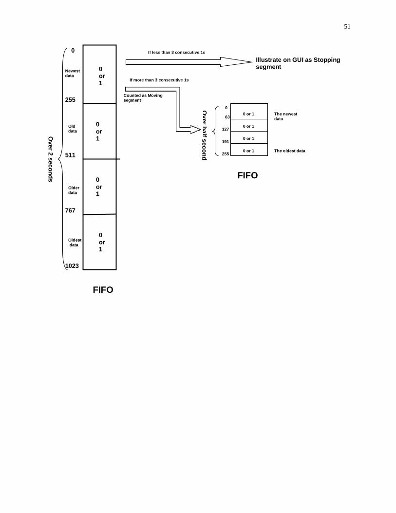
51

0

1023

255

511

767

127

63

0

191

255

If more than 3 consecutive 1s

0 or 1

0 or 1

0 or 1

0 or 1

0 or 1

0 or 1

0 or 1

0 or 1

Over 2 seconds

Over half second

Newest data

Old data

Older data

Oldest data

FIFO

If less than 3 consecutive 1s

Illustrate on GUI as Stopping segment

FIFO

The newest data

The oldest data

Counted as Moving segment

52

Figure 6.5: A schematic view of online implementation of step detection algorithm.

0 or 1

0 or 1

0 or 1

0 or 1

0 or 1

0 or 1

0 or 1

0 or 1

0 or 1

0 or 1

0 or 1

0 or 1

0 or 1

0 or 1

0 or 1

0 or 1

0

1023

Over 2 seconds

If less than 3 consecutive 1s

If more than 2 consecutive 1s

Illustrate on GUI as Stance phase

Will be counted as Swing phase Searching for peaks in

Swing phase

53

Chapter7: Fixed Point Arithmetic In order to adapt the real-time step detection algorithm for implementing in microcontroller

MSP430 system which has no floating point unit (FPU) and then implementing algorithm on the

iNODE system, the data format should be transformed from floating point numbers into fixed

point numbers by changing the magnitude of data into fixed point numbers and employ fixed

point arithmetic. Due to the penetrating role of the data formats on the accuracy of

implementation, the difference between floating point and fixed point has to be determined. A

short introduction about fixed point numbers and arithmetic will be provided in the first part of

this chapter. Later the transformation of the developed algorithm into fixed point arithmetic will

be presented. Determination of accuracy and overflow errors has been done using MATLAB

Fixed Point Toolbox. With these results this chapter will be closed.

7.1 Fixed point numbers A fixed-point number represents a real data type for a number that has a fixed number of digits

after and sometimes before the radix point (decimal notation) also able to be represented using

integer arithmetic. The numbers are called fixed point numbers, because the radix point is always

at the same, fixed, point in every number. Floating point has a sliding window of precision,

which provides a large dynamic range and high precision. Since the embedded system can only

process bits, all the fractional and integer numbers must be represented by collection of bits (0 or

1), hence the number system naturally used in embedded system is the binary system. A

collection of N bits has N2 possible states. This can be achieved from elementary counting

theory, which tells us that there are two possibilities for the first bit, two possibilities for the next

bit, and so on until the last bit, resulting in 2×2×2… = N2 possibilities. An N-bit binary word

corresponds to an integer between 0 and 12 −N . In order to represent the negative (signed) values,

naturally we need to introduce the two's complement representation and corresponding operations

to implement arithmetic on the numbers represented in the two's complement format. In 2's

complement representation, an N-bit word represents integers from − ( 12 −N ) to 12 −N −1. In Fig.

7.1 some examples of numbers in two’s complement are given.

54

Binary Decimal

00000000 0

00000001 1

01000000 64

01111111 127

10000000 -128

10000001 -127

11000000 -64

11111111 -1

Figure 7.1: Some examples of numbers in two’s complement

7.2 Q-format For implementing the numerical representation of a fixed point number, specifying the location

of the radix point is needed, which causes to introducing Q-format. The Q-format shows the

location of the radix point by informing number of the existing bits to the right and also to the left

of the radix point. If we have an N-bit binary word with MSB as the sign bit, we have N -1 bits to

represent the fraction. It is known as, the number has Q-(N−1) format. For example, Q10.5

describes a number with 10 magnitude bit and 5 fractional bits in a 16 bit word.

In the following table (Fig. 7.2) some Q-7 format binary numbers and the conversion to decimal

numbers is given:

Binary Decimal 01001101 .6015625

11100100 -.21875

01111001 .9453125

10001011 -.9140625 Figure 7.2: Some Q-7 binary numbers and their conversion to decimal numbers

7.3 Numerical operation Numerical operations of numbers in two’s complement are included of :

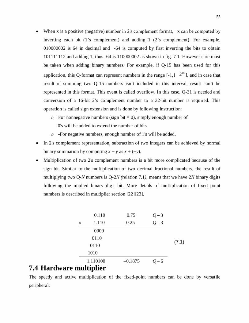
55

• When x is a positive (negative) number in 2's complement format, −x can be computed by

inverting each bit (1’s complement) and adding 1 (2’s complement). For example,

010000002 is 64 in decimal and -64 is computed by first inverting the bits to obtain

101111112 and adding 1, thus -64 is 110000002 as shown in fig. 7.1. However care must

be taken when adding binary numbers. For example, if Q-15 has been used for this

application, this Q-format can represent numbers in the range [-1,1− 152 ], and in case that

result of summing two Q-15 numbers isn’t included in this interval, result can’t be

represented in this format. This event is called overflow. In this case, Q-31 is needed and

conversion of a 16-bit 2’s complement number to a 32-bit number is required. This

operation is called sign extension and is done by following instruction:

o For nonnegative numbers (sign bit = 0), simply enough number of

0's will be added to extend the number of bits.

o -For negative numbers, enough number of 1's will be added.

• In 2's complement representation, subtraction of two integers can be achieved by normal

binary summation by computing x − y as x + (−y).

• Multiplication of two 2's complement numbers is a bit more complicated because of the

sign bit. Similar to the multiplication of two decimal fractional numbers, the result of

multiplying two Q-N numbers is Q-2N (relation 7.1), means that we have 2N binary digits

following the implied binary digit bit. More details of multiplication of fixed point

numbers is described in multiplier section [22][23].

(7.1)

7.4 Hardware multiplier The speedy and active multiplication of the fixed-point numbers can be done by versatile

peripheral:

61875.0110100.1

1010011001100000

325.0110.1375.0110.0

−−

−−×−

Q

QQ

56

Hardware multiplier implemented in MSP430. Its activity doesn’t interfere with the CPU’s

activities, since the hardware multiplier is a peripheral but not part of the MSP430 CPU. The

hardware multiplier supports signed multiply and signed multiply accumulate. It has two 16-bit

operand registers, OP1 and OP2, and three result register, RESLO, RESHI, and SUMEXT.

Sumext contains the extended sign of the results. The result of fixed point multiplication could

potentially have as many bits as the sum of the number of bits in the two operands. The lower 16-

bit of the result is stored in RESLO, and RESHI holds the higher 16 bits of the calculation result.

In order to fit the result into the same number of bits operand, the result must be truncated. The

choice of which bits have to be kept is thus very important. When multiplying two fixed point

numbers with the same format, for instance with Ι integer bits, and Q fractional bits, the answer

could have up to Ι2 integer bits, and 2Q number of fractional bits. The middle bits: the Ι -

number of least significant integer bits, the Q number of most significant fractional bits will be

kept. Fractional bits lost below this value represent a precision loss which is common in

fractional multiplication. If non-zero integer bits are lost, the value will be radically inaccurate.

This is considered to be an overflow or underflow, which need to be avoided in embedded

calculation. The hardware multiplier does not detect the underflow and overflow automatically.

Even if the error is detected by the user software, it is hard to handle this error promptly and

appropriately. Therefore it is recommended to detect and avoid such overflow and underflow by

usage of appropriate result word size and radix point, proper scaling factor and magnitude

limiting of intermediate results when initiating programming [24][25].

7.5 Precision Loss and Error Due to the finite number of word length in fixed-point numbers, there are possibilities for

precision loss and errors occurrence which can include of:

7.5.1 Truncation error In order to fit the answers of fixed-point operations into the same number of bits as the operands,

the result must be truncated. For example, 1.79 • 1.79 in Q4.4 format which means four bits after

the binary point is represented 0001.1101 • 0001.1101 = 0011.0100 1001. Rounding the binary

number causes discarding bits to the right of its LSB which will give 0011.0100 (3.25), whereas

the real results is 3.2041. The error rate of this result is 1.42%. With increasing the number of

operation, the error rate will increase which leads to more precision loss. Truncation error also is

known as Quantization error and roundoff error. Generally, in fixed-point arithmetic, truncation

or roundoff errors are independent of the magnitude of the original unquantized numbers [26].

57

7.5.2 Overflow A computation with a result number, larger than the defined dynamic range of the system or

resulting in an output with an incorrect sign or sum is called overflow. It is also called register

overflow, large signal limit cycling or saturation. For example, 16.9684 x 16 in Q8.8 format is

equal to 0001 0000. 1111 0111 • 0001 0000. 0000 0000 = 0001 0000 1111. 0111 0000 0000

0000. Discarding the left-most 4 bits 0001 and the right-most 4 bits, the middle 16 bits will be

0000 1111. 0111 0000, which is equal to 15.4375. Nevertheless, the real product is 271.4368.

Likewise the erroneous sign is yielded in multiplication of signed number when the left-most bit,

which has a negative weight in the two’s complement number is lost.

7.5.3 Underflow Underflow is another term for overflow error. The errors mentioned above, can be generated

through the operation chains. By selecting the Q-format carefully, the precision loss can be

reduced or prevented.

7.6 Division While doing the division operation on fixed point numbers, it would cause the precision error.

Avoiding these errors is a big challenge in this area. There are some methods such as using

Horner 32 or implementing the Arctangent function for achieving the best Q-format and word

length, however, using all of these methods each have their own pre-conditions. One of the

conveniences of our method is its simplicity which causes having denominator in power of 2, in

the division operation. Having a power of 2 number in denominator, doesn’t need the division

operation, and can be done by shift operation.

7.7 Defining appropriate data format: A common problem in fixed-point development is to determine the correct scaling and data types

for a fixed-point algorithm. For example, if we are using a 16:16 fixed point we have one of two

choices for division, a 32 bit or a 64 bit division. The 32 bit divide looses precision in over 75

percent of cases (assuming a random distribution), however the 64 bit divide is over 4 times

slower.

In order to find the best Q-format and wordlength and also avoiding overflow and underflow

error, fixed point Toolbox of MATLAB is used. Fixed-Point Toolbox in MATLAB provides

fixed point data types and also arithmetic. This toolbox lets user to design fixed-point algorithms

using MATLAB syntax and execute them at compiled C-code speed. These algorithms can be

58

reused in Simulink and pass fixed-point data to and from Simulink models, facilitating bit-true

simulation, implementation, and analysis. This toolbox also enables the user to generate test

sequences for fixed-point software and hardware verification.

So, after determining the scaling of the fixed-point algorithm, this information can be used in

Embedded MATLAB to automatically generate fixed-point C code from current MATLAB

algorithm.

Fortunately, our step detection algorithm mostly deals with 0 and 1, which means no need to

conversion from floating to fixed point. The main part of this algorithm is based on variance

calculation, including mean calculation. The rest of the algorithm is based on different buffers

containing zeros and ones depending on the variance exceed the threshold value or not. So for the

fixed point implementation the greatest challenge is about variance function which includes

multiple division, multiplication and summation operation. However, as it was mentioned above,

this algorithm is designed in a way to get a power of 2 number in the denominator of the

divisions which can be done by counting the bits and perform a bit shift right.

By applying fixed point toolbox in MATLAB, the effect of using fixed point variables for

calculating mean and variance is tested. For these purpose two programs are developed to

determine what type of fixed point definition is required for getting satisfying result. As a

confirmation, the results have been compared with double precision results. The codes of these

programs can be found in Appendix.

According to the codes of these two programs, first calculation of mean and variance function is

considered by computing the mean by bit shifting and put the sum up values in the variable fp1,

calculating the absolute deviation from mean and save it in the vector fp2, also calculation of the

mean by shifting and summing up the squared deviation and putting the values in the variable

fp3.

• fp1 = numerictype('Signed',0,'WordLength', 32, 'FractionLength', 0);

• fp2 = numerictype('Signed',0,'WordLength', 32, 'FractionLength', 0);

• fp3 = numerictype('Signed',0,'WordLength', 16, 'FractionLength', 0);

• mean = numerictype('Signed', 0, 'WordLength', 16, 'FractionLength', 0);

• var = numerictype('Signed', 0, 'WordLength', 32, 'FractionLength', 0); - No over- or underflow

- Truncation error negligible

59

After programming the desired variance function via fixed point toolbox of MATLAB, and using

acceleration data which has been recorded by iNODE system, the appropriate word length,

fraction length and signed/unsigned has been found without causing any overflow or underflow

for mean, variance and fp1, fp2, fp3.[27]

According to the codes in Appendix, results have been compared with double precision

arithmetic.

60

Chapter8: Conclusion and future work The reduced phase coordination between respiration and locomotion can be indicator of

Parkinson’s disease (PD) degree. It leads to interest in long-term online monitoring and analysis

of steps and also in further studies, of phase coordination between locomotion and respiration for

the application during both occupational therapy and daily routines outside laboratories. For this

intention, our group in ZEL, have designed low-cost, miniature, lightweight, patient comfort,

wireless and intelligent sensor nodes which builds up a distributed intelligent sensor network.

These sensor nodes are unique solution for this specific application of neurological research.

Extreme energy-efficiency has been concerned during development of intelligent Network

Operating DEvice sensor node (iNODE), since the size of the battery need to be reduced and

prolonged batter life is desired. The ultra-miniature design of the sensor node maximizes patient

comfort. These sensor nodes along with specifically selected sensor components allow non-

invasive and continuous health monitoring for locomotion and respiration with sufficient patients

comfort. For clinical application, the sensor node for step detection realizes the function of

identifying the moment when a step has been made, in addition to monitoring the step signals.

Before decision of sensors for step detection, technical overview of miscellaneous sensors for

monitoring activation has been covered. Three-dimensional accelerometer is popularly employed

in gait analysis. A lightweight algorithm is developed for automatic step detection in the 3D

acceleration signals. FSR sensor offers an alternative which is a convenient and inexpensive

solution for accurate detection of gait events. It does not restrict patients’ activity for its tiny

thickness and small size. However, in some cases signals which are taken from FSR sensors are

not accurate enough, and are not able to show all the details of movements comparing with

signals from 3D accelerometers.

The iNODE sensor nodes for step detection and respiratory monitoring have been developed. It is

highly miniaturized as a 20x20x20 mm compact cube. The hardware board of the iNODE sensor

node is constructed as modules, which allows the main board containing MSP430 micro-

controller to mount with various physiological sensors. Asides from data logging, iNODEs

analyze the step and respiratory signals automatically. To implement the step detection algorithm

on MSP430, conversion from floating point to fixed point numbers has been used. Fixed-point

implementation, constrained computing resource, operation in frame sequence and time-constrain

in real-time computation. In this work, a great effort has been invested to optimize the

61

algorithms, simplify the computational operations and reduce computational overhead for real-

time step detection. This system for step detection has been evaluated by healthy volunteers and

PD patients in cooperation with Centre for Sleep and Rehabilitation Research of Clinic Ambrock

for Neurology, Germany. The algorithm for automatic step detection using accelerometer is

performed on the PD patients’ data. In addition to the accelerometer, FSR sensor is also tested in

the PD patients. It has been proved with clinical data, that precise step events can be detected

from the FSR signal for the simple features of the signals. The clinical results recorded while the

patients were walking on the treadmill. The accelerometer, FSR sensors have been tested on the

PD patients during clinical experiments. Furthermore, the FSR signal collected from patients

does not differ from the data measured by healthy subjects. These methods give overall robust

and high performance for the off-line analysis of clinical dataset in this study.

A number of experiments have been run to test the online calculation of step detection algorithm.

The raw data of fixed-point results is compared with the floating-point results via fixed point

toolbox of MATLAB. In micro-controller 8 millions of calculations can be done in 1 second.

According to our computations, approximately 750,000 calculations in 1 second are needed for

this algorithm which means using 1/10 times by the memory of micro-controller. Considering

limited memory space of MSP430, algorithm is fast enough from the computational standpoint.

After this stage, the data is ready for implementing in micro controller. Hopefully, this part of

project will be done during next 1-2 months by the rest of the group which will not remain too

much intellectual work to do and it is just the matter of time, and also the wireless

communication interface will be integrated into these current iNODEs for step and respiratory

monitoring. After assembling of flexible printed circuit board (PCB) for the new version is

completed, it will be introduced in clinical measurements.

8.1 Perspectives In the next stage, the iNODE system will be employed in clinical measurements to improve the

patient’s safety and comfort. Further studies of different medical conditions using this mobile

wireless system will be conducted. The first application of our system in the Centre for Sleep and

Rehabilitation Research, Hagen-Ambrock, will be the recording of the locomotor respiratory

coordination of PD patients while carrying out occupational therapy on a treadmill.

This study focuses on questions whether this coordination will be improved in course of the

rehabilitation and whether it can be a measure for the rehabilitation effect. Secondly, results of

the locomotion coordination in condition of free walking using this system will be compared with

62

measurements recorded while walking on treadmill. After evaluation of the system in these

studies, it will be introduced in long-term recording in order to investigate circadian rhythm of

the locomotion coordination in free-living condition during daily life, which will be supervised

by our clinical partner.

63

Abbreviations ADC Analog-to-Digital Converter

aNODE autarkic Network Operating DEvice

CPU Central Processing Unit

DMA Direct Memory Access

DAC Digital to Analogue Converter

DAQ Data Acquisition

DC Direct Current

FFT Fast Fourier Transform

FIR Finite Impulse Response

FRABOS FRAme Based Operating System

FSR Force-Sensing Resistor

FPU Floating Point Unit

GUI Graphical User Interface

IEEE Institute of Electrical and Electronics Engineers

IIR Infinite Impulse Response

iNODE intelligent Network Operating Device

LSB Least Significant Bit

MSB Most Significant Bit

op-amp operational amplifier

PD Parkinson’s Disease

PTM Pan-Tompkins Method

Sqrt Square root

STD Standard Deviation

64

TMM Template-Matching Method

Cµ micro-controller

USB Universal Serial Bus

Var Variance

65

Bibliography

[1] http://parkinsoninfo.org

[2] http://www.merck.com/mmhe/sec06/ch091/ch091d.html

[3] S.Schiermeier, D. Schäfer, and M.E. Schläfke, Breathing and locomotion in patients with

Parkinson’s disease. Eur. J. Physiol., 443:67-71, 2001.

[4] Mario Schlösser, Andreas Schnitzer, Hong Ying, Carmen Silex, Michael Schiek

iSANLA: intelligent Sensor and Actuator Network for Life science Applications

Central Institute for Electronics, ZEL, Forschungszentrum Juelich, Germany, 2008

[5] Susan D. Vincent, Cara L. Sidman, "Determining Measurement Error in Digital

Pedometers", Measurement in Physical Education and Exercise Science 7 (1): 19–24.

doi:10.1207/S15327841MPEE0701_2., 2003

[6] C G Ryan, P M Grant, W W Tigbe, M H Granat, "The validity and reliability of a

novel activity monitor as a measure of walking", British Journal of Sports Medicine 40,

2006

[7] American college of SportsMedicine, www.acsm.org

[8] K. M. Culhane1, M. O’Connor2, D. Lyons2 and G. M. Lyons , Accelerometers in

rehabilitation medicine for older adults, Biomedical Electronics Laboratory, Department of

Electronic and Computer Engineering, University of Limerick, Limerick, Ireland

66

Rehabilitation Centre, St. Camillus’ Hospital, Limerick, Ireland

[9] K. Aminian, B. Najafi,C. Büla, P.-F. Leyvraz and Ph. Robert, AMBULATORY GAIT

ANALYSIS USING GYROSCOPES, 1 Swiss Federal Institute of Technology (EPFL),

Metrology Laboratory, Lausanne, Switzerland

2 Service of Geriatric Medicine, CHUV & CUTR Sylvana, Epalinges, Switzerland

3Hôpital Orthopédique de la Suisse Romande, Lausanne, Switzerland

[10] Masaki Hirasawa, Hidetaka Okada, and Makoto Shimojo, The Development of the Plantar

Pressure Sensor Shoes for Gait Analysis, Department of Mechanical Engineering and

Intelligent Systems, The University of Electro-Communications, 1-5-1 Chofugaoka, Chofu,

Tokyo 182-8585, Japan [Received September 29, 2007; accepted December 17, 2007]

[11] Tietze and Ch. Schenk., Halbleiter Schaltungs-technik, chapter 6: Kippschaltungen, pages

611–618, Springer, 12. Ausgabe, 2002

[12] G. Hegewald, Ganganalytische Bestimmung und Bewertung der Druckverteilung unterm

Fuss und von Gelenkwinkelverl¨aufen, Dissertation, Institute fur

Rehabilitationswissenschaften, Humboldt Universit at zu Berlin, Germany, 1999

[13] Tietze and Ch. Schenk., Halbleiter Schaltungs-technik, chapter 6: Kippschaltungen, pages

611–618, Springer, 12. Ausgabe, 2002

[14] H. Ying, M. Schlösser, A. Schnitzer, S. Leonhardt and M. Schiek, Distributed Intelligent

Sensor Network for Neurological Rehabilitation Research, Central Institute for Electronics,

Research Centre Jülich, Germany, Philips Chair for Medical Information Technology,

67

RWTH Aachen University, Germany, 2008

[15] R. M. Rangayyan, Biomedical Signal Analysis, chapter 4: Event Detection, pages 466–471.

IEEE Press Series on Biomedical Engineering, 2002.

[16] J. Pan and W. Tompkins., A real-time QRS detection algorithm, IEEE Transactions on

Biomedical Engineering, 32:230–236, 1985.

[17] R. Farre, J. M. Montserrat, and D. Navajas, Noninvasive Monitoring of Respiratory

Mechanics during Sleep. Eur Respir J 2004, 24:1052 – 1060, 2004

[18] Jonghee Han, Hyo Sun Jeon, Beom Suk Jeon, Kwang Suk Park, Gait detection from three

dimensional acceleration signals of ankles for the patients with Parkinson’s disease

[19] Jonghee Han, Hyo Sun Jeon, Beom Suk Jeon, Kwang Suk Park,

Gait detection from three dimensional acceleration signals of ankles for the patients with

Parkinson’s disease

[20] David Kempe , Online Algorithms, Lecture Notes for CSCI 570, December 1, 2006

[21] Buffer Operations in GIS, Nagapramod Mandagere, Graduate Student, University of

Minnesota, npramod@cs.umn.edu

68

[22] G. R. Whilson., Embedded System and Computer Architecture, chapter 4:

[23] R. C. Cofer and B. Harding, Fixed-Point DSP and Algorithm Implementation,

ESC Boston Conference, Oct. 2006.

[24] Texas instruments, MSP430 User’s Guide, 2006. SLAU049F

[25] Fixed point arithmetic, http://en.wikipedia.org/wiki/fixed-point-arithmetic.

[26] The control handbook, Editor: William S. Levine, A CRC Handbook published in

cooperation with IEEE Press; page 304.

[27] Fixed-Point Concepts, Fixed-Point Toolbox-Matlab documentation.

[28] Signal Processing (SP) Toolbox, Matlab documentation.

[29] Introduction to the Filter Design and Analysis Tool (FDATool). MATLAB documentation

[30] guide initiates the GUI design environment (GUIDE), MATLAB documentation

69

[31] Texas instruments, MSP430 User’s Guide, 2006. SLAU049F

[32] Fixed point arithmetic, http://en.wikipedia.org/wiki/fixed-point-arithmetic.

[33] The control handbook, Editor: William S. Levine

A CRC Handbook published in cooperation with IEEE Press; page 304.

[34] S.Schiermeier, D. Schäfer, and M.E. Schläfke, Breathing and locomotion in patients with

Parkinson’s disease. Eur. J. Physiol., 443:67-71, 2001.

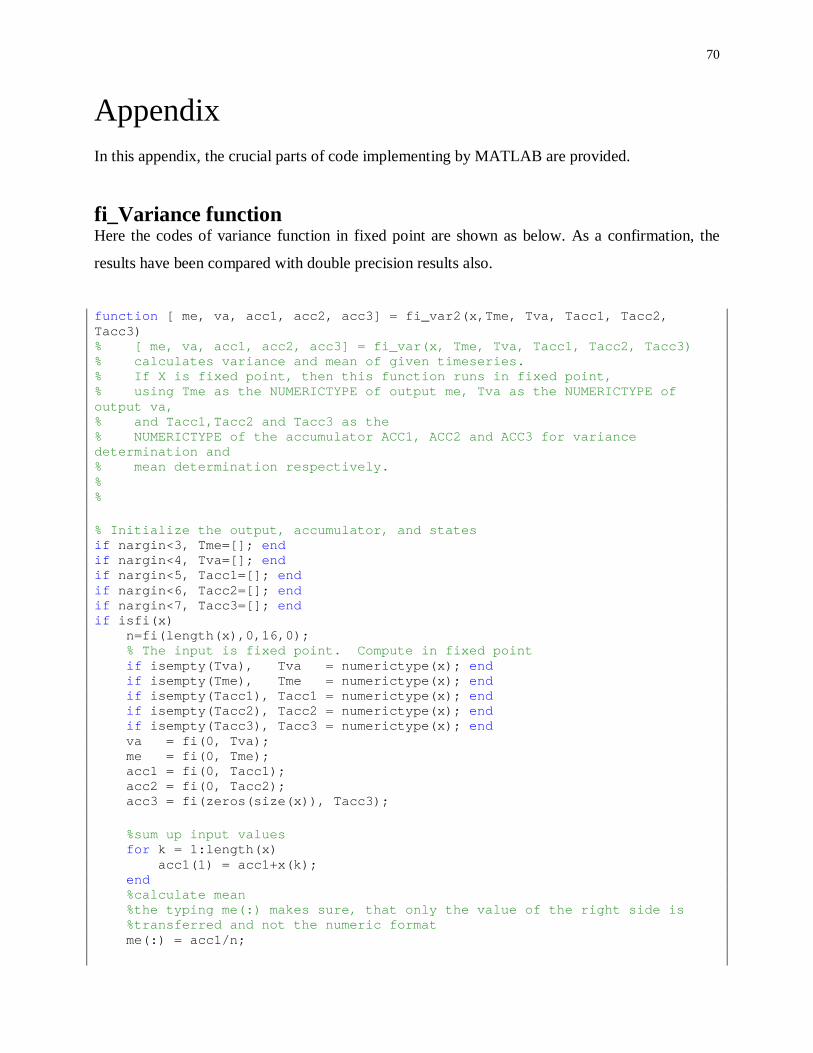
70

Appendix In this appendix, the crucial parts of code implementing by MATLAB are provided.

fi_Variance function Here the codes of variance function in fixed point are shown as below. As a confirmation, the

results have been compared with double precision results also.

function [ me, va, acc1, acc2, acc3] = fi_var2(x,Tme, Tva, Tacc1, Tacc2, Tacc3) % [ me, va, acc1, acc2, acc3] = fi_var(x, Tme, Tva, Tacc1, Tacc2, Tacc3) % calculates variance and mean of given timeseries. % If X is fixed point, then this function runs in fixed point, % using Tme as the NUMERICTYPE of output me, Tva as the NUMERICTYPE of output va, % and Tacc1,Tacc2 and Tacc3 as the % NUMERICTYPE of the accumulator ACC1, ACC2 and ACC3 for variance determination and % mean determination respectively. % % % Initialize the output, accumulator, and states if nargin<3, Tme=[]; end if nargin<4, Tva=[]; end if nargin<5, Tacc1=[]; end if nargin<6, Tacc2=[]; end if nargin<7, Tacc3=[]; end if isfi(x) n=fi(length(x),0,16,0); % The input is fixed point. Compute in fixed point if isempty(Tva), Tva = numerictype(x); end if isempty(Tme), Tme = numerictype(x); end if isempty(Tacc1), Tacc1 = numerictype(x); end if isempty(Tacc2), Tacc2 = numerictype(x); end if isempty(Tacc3), Tacc3 = numerictype(x); end va = fi(0, Tva); me = fi(0, Tme); acc1 = fi(0, Tacc1); acc2 = fi(0, Tacc2); acc3 = fi(zeros(size(x)), Tacc3); %sum up input values for k = 1:length(x) acc1(1) = acc1+x(k); end %calculate mean %the typing me(:) makes sure, that only the value of the right side is %transferred and not the numeric format me(:) = acc1/n;

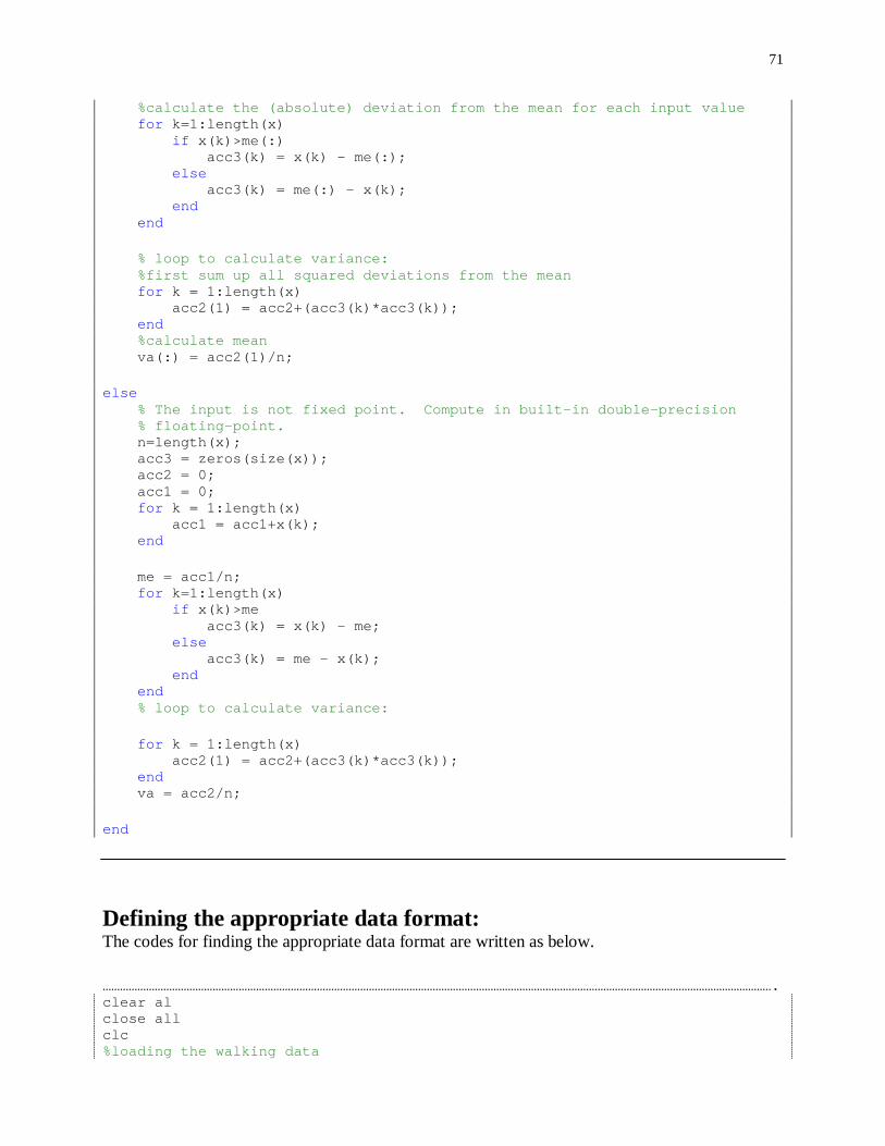
71

%calculate the (absolute) deviation from the mean for each input value for k=1:length(x) if x(k)>me(:) acc3(k) = x(k) - me(:); else acc3(k) = me(:) - x(k); end end % loop to calculate variance: %first sum up all squared deviations from the mean for k = 1:length(x) acc2(1) = acc2+(acc3(k)*acc3(k)); end %calculate mean va(:) = acc2(1)/n; else % The input is not fixed point. Compute in built-in double-precision % floating-point. n=length(x); acc3 = zeros(size(x)); acc2 = 0; acc1 = 0; for k = 1:length(x) acc1 = acc1+x(k); end me = acc1/n; for k=1:length(x) if x(k)>me acc3(k) = x(k) - me; else acc3(k) = me - x(k); end end % loop to calculate variance: for k = 1:length(x) acc2(1) = acc2+(acc3(k)*acc3(k)); end va = acc2/n; end Defining the appropriate data format: The codes for finding the appropriate data format are written as below. ……………………………………………………………………………………………………………………………………………………………………………………………………………. clear al close all clc %loading the walking data

72

load 002.mat tt=GesamtDaten(512:2:end,1); data = GesamtDaten(512:2:end,3); %make sure that no DatatypeOverride is activated %Data type override only occurs when the fi constructor function is called. fipref('DataTypeOverride','ForceOff'); %define measurement data as fixpoints unsigned 16 bit Integer %and take the first 256 data points x=fi(data(1:256),0,16,0); %double precision data for control x_d = data(1:256); t_d = tt(1:256); %plot data plot(t_d,x); grid on; drawnow %test with double precision [my_mean_d, my_variance_d, acc1_d, acc2_d] = ... fi_var2(x_d, length(x)); my_mean_d my_variance_d %set parameters of fixed point toolbox %activate warnings to see over- and underflow events warning on fi:overflow warning on fi:underflow warning on backtrace fipref('LoggingMode','on'); % fipref('LoggingMode','off'); %Define fixed point quantities Tme = numerictype('Signed', 0, 'WordLength', 16, 'FractionLength', 0); Tva = numerictype('Signed', 0, 'WordLength', 32, 'FractionLength', 0); Tacc1 = numerictype('Signed', 0, 'WordLength', 32, 'FractionLength', 0); Tacc2 = numerictype('Signed', 0, 'WordLength', 16, 'FractionLength', 0); Tacc3 = numerictype('Signed', 0, 'WordLength', 16, 'FractionLength', 0); %calculate using these fixed point definitions [my_mean, my_variance, acc1, acc2, acc3] = ... fi_var2(x, Tme, Tva, Tacc1, Tacc2, Tacc3); %compare the output my_mean my_variance %the next demonstrates a method to log all over- and underflow events and create a logreport fipref('DataTypeOverride','ScaledDoubles'); x=fi(data(1:256),0,16,0);

73

[my_mean_sd, my_variance_sd, acc1_sd, acc2_sd, acc3_sd] = ... fi_var2(x, Tme, Tva, Tacc1, Tacc2, Tacc3); %now show the report of min and max values logreport(my_mean_sd, my_variance_sd, acc1_sd, acc2_sd, acc3_sd) …………………………………………………………………………………………………………………………………………………………………………………………………………….

Blekinge Tekniska Högskola SE–371 79 Karlskrona Tel.vx 0455-38 50 00 Fax 0455-38 50 57