Proceedings of Machine Learning Research 71:56–65, 2017 KDD 2017: Workshop on Anomaly Detection in Finance

Real-time anomaly detection system for time series at scale

Meir Toledano, Ira Cohen, Yonatan Ben-Simhon, Inbal Tadeski{meir, ira, yonatan, inbal}@anodot.com

Anodot Ltd., HaTidhar 16, Ra’anana, Israel

Abstract

This paper describes the design considerations and general outline of an anomaly detectionsystem used by Anodot. We present results of the system on a large set of metrics collectedfrom multiple companies.

Keywords: Anomaly detection, time series modeling, high scalability, seasonality detec-tion

1. Introduction

A challenge, for both machines and humans, is identifying an anomaly. Very often theproblem is ill-posed, making it hard to tell what an anomaly is. Fortunately, many metricsfrom online systems are expressed in time series signals. In time series signals, an anomalyis any unexpected change in a pattern in one or more of the signals.

There are obvious things that most people agree on of what it means to be the same,and that’s true for time series signals as well, especially in the online and financial worldwhere companies measure number of users, transaction volume and value, number of clicks,revenue numbers and other similar metrics. People do have a notion of what “normal” is,and they understand it because, in the end, it affects revenue. By understanding “normal”,they also understand when something is “abnormal”. Thus, knowing what an anomaly isisn’t completely philosophical or abstract.

Anomaly detection has been an active research area in the fields of statistics and ma-chine learning. Temporal methods, going all the way back to Holt-Winters Chatfield (1978),classical ARIMA and seasonal ARIMA models Chatfield (2016), clustering techniques fordiscovering outliers in time series and other types of data, and more, have been researchedand suggested over the years Krishnamurthy et al. (2003)Chandola et al. (2009). But,when building a production ready anomaly detection system, what are the main designprinciples? It depends on the needs and use case.

Based on our experience, there are some main design considerations when building anautomated anomaly detection system:

1. Timeliness: How quickly does the company need to an answer to determine if something is ananomaly or not? Does the determination need to be in real-time, or is it okay for the systemto determine it was an anomaly after a day, week, month or year has already passed?

2. Scale: Does the system need to process hundreds of metrics, or millions? Will the datasets beon a large scale or a relatively small scale?

3. Rate of change - Does the data tend to change rapidly, or is the system being measuredrelatively static?

c© 2017 M. Toledano, I. Cohen, Y. Ben-Simhon & I. Tadeski.

KDDADF2017

4. Conciseness: If there are a lot of different metrics being measured, must the system producean answer that tells the whole picture, or does it suffice to detect anomalies at each metriclevel by itself?

5. Robustness without supervision: Can the system rely on human feedback in some of themodeling choices (e.g., choice of algorithms and/or parameters for data streams), or does ithave to be produce robust results in a completely unsupervised settings?

For most use cases related to online businesses in general, and finance in particular, therequirements from an anomaly detection system is to produce near real time detection atvery large scale, while producing concise anomalies and being able to adapt to normalchanges in data behavior. Given the amount of signals such businesses produce, a systemmust work robustly with no human intervention.

In this paper we’ll describe the key components of the Anodot anomaly detectionsystem, a system which discovers anomalies today for about 50 different companies andover 120 million time series metrics reporting constantly. We’ll explain the choices ofalgorithms and architecture required for such a system to meet the design principles outlinedabove. We’ll show results on real data from companies in the financial areas, demonstratingdetection of fraudulent bots, and other issues.

2. Time series modeling and anomaly detection

To meet all of the requirements stated above - robustly detecting anomalies in (near) real-time, at very large scale, while being adaptive to ever-changing data and producing conciseanomalies, we built a learning system that follows the following five steps:

1. Universal Metrics collection: The ability to collect and analyze millions to billions of timeseries metrics in real time with zero manual configuration.

2. Normal behavior learning: The first step towards identifying anomalies is learning a modelof what is considered normal and devising a statistical test to determine that data points areanomalous if they are not explained by the model

3. Abnormal behavior learning: Once an anomaly is discovered, it is important to understandboth its significance and its type. A significant anomaly is one that is more “surprising”compared to past anomalies. Learning is required to learn the significance of each anomalybased on various attributes describing the anomaly.

4. Behavioral topology learning: To show concise anomalies, the relationships between the po-tentially millions of time series inputs needs to be learned. Learning the relationship canbe achieved by observing various aspects of the metrics behavior and applying clusteringalgorithms to discover similarities of those behaviors.

5. Feedback-based learning: It is feasible to obtain small amounts of supervision in labelinganomalies to be true or false positives. These feedbacks are used to update the models learnedin the previous steps.

3. Learning normal behavior

Learning the normal behavior of a time series Xt amounts to learning the temporal dynam-ics and distribution of the time series PNormal(Xt|Xt−1, ..., X0) such that we can determinethe likelihood of the data point Xt+1 to have originated from PNormal(Xt+1). There areseveral challenges in robustly learning the distribution for any time series (without anysupervision).

57

KDDADF2017

Figure 1: Example of six different types of time series signals

First one needs to choose the right parametric (or non-parametric) model before esti-mating PNormal. Second, account for seasonal behavior that may or may not be presentin the signal. Last, be able to adapt to changes in the behavior, even in the presence ofanomalies.

3.1. Choosing the best model

There are a variety of models that capture and produce such a distribution, each fittingdifferent types of time series signal behaviors. For example, time series models such as Holt-Winters, ARIMA models, and Hidden Markov Models, all capture temporal dynamics of atime series and produce a generative distribution for predicting the ranges of future values.But can these models be used for any type of signal? The answer is no - each model comeswith its own assumptions, affecting what type of signal can be fitted well with it. Forexample, ARIMA and Holt-Winters models assume the the time series is ergodic, with anoise model that is Gaussian. A Markov model makes assumption on the memory of theprocess (current state depends only on previous state), and so on.

Based on about 120 million different time series signals, originating from a variety ofbusinesses (from online financial services to manufacturing sensors), we discovered multipletypes of behaviors that require separate types of models. Figure 1 demonstrates six maintypes of time series: Stationary “smooth”, irregularly sampled, discrete valued, “sparse”,“step”, and multi-modal. While approximately 40% of metrics are stationary, many fallunder the other types, requiring special models. For example, “sparse” metrics are signalsthat are mostly 0, but occasionally see a value different than 0. E.g., a signal countingthe number of transactions related to a stock at each 5 minute window - may be 0 mostof the time but non-zero values are only anomalies if larger than usual when the metricis not zero. Models such as Holt-Winters, would flag each non-zero value as an anomaly,producing many false positives. Similar examples demonstrate the need for a special modelfor each type.

The first step before learning a model of normality for a metric is therefore a classifierthat decides for each metric, based on its history, what would be the best model for it.

Once we choose the model that would describe the metric the best, we must fit thebest model parameters for it. Depending on the type of model, this step may take differentforms - we use maximum likelihood estimation (MLE) for this step. While describing themaximum likelihood estimation method for each of the models is beyond the scope of thispaper, there is a very important step that precedes the MLE, which is detecting whetherthe signal has seasonal patterns or not, and which seasonal patterns.

58

KDDADF2017

Figure 2: Example of periodic time series (with a weekly seasonal pattern)

3.2. Seasonality detection

The purpose of seasonality detection is to automatically find the seasonal patterns presentin the time series. In the context of large scale anomaly detection system, we are facing toseveral challenges:

1. In the context of business data, typical seasonal periods are linked to human activity : weekly,daily, hourly, etc. The range of possible seasons is large : from 103s to 106s, which is threeorder of magnitude - this imposes a challenge to standard algorithms.

2. An algorithm must be robust to anomalies. One cannot assume that the anomalies are notpresent in the data used to detect seasonal patterns.

3. Multiple seasonal patterns in the time series, at low and high frequencies are challengingas high frequency seasonal patterns may prevent accurate detection of the lower frequencypatterns (which we care about the most for time series modeling).

4. An algorithm must be efficient in CPU and memory, otherwise it cannot be applied to millionsof metrics.

5. The algorithm must be robust to various types of unexpected conditions, such as missing data,pattern changes, etc.

3.2.1. Bank filter

To tackle the first challenge of having several order of magnitude of possible seasonalpattern periods (from minutes to weeks, and potentially more), we adopted a “Divideand Conquer” strategy on the spectrum. We split the series by applying three differentband pass filters (three is for finding patterns from minutes to weeks). A Band pass filteroperates on the Fourier space by selecting only a band of frequencies to be presents inthe outputs, removing all other components. In our system we have three different filtersconceived to extract the weekly band, the daily band and the hourly band. The numberand the definition of bands are based on statistical analysis of our data-set. After applyingthe three filters on the times series, we have three different time series: Time series slowband, Time series medium band and Time series fast band. Our implementation uses thefifth order Butterworth filter. The effect of the filter bank can be seen in Fig. 3(a) for themedium band and Fig. 3(b).

59

KDDADF2017

(a) the slow band (b) the medium band

Figure 3: Effect of the filtering on the original series Fig. 2.

Figure 4: The ACF for the slow band, series Fig. 3(a).

3.2.2. Fast autocorrelation function

For each series produced by the filter bank we look for a prominent seasonal pattern, ordetermine that it does not contain one. For performing this task use the autocorrelationfunction (ACF) which is a function of the lag τ :

ρ(τ) = Cor(Xt, Xt+τ ) =E[(Xt − E[Xt])(Xt+τ − E[Xt+τ ])]√

Var[Xt]Var[Xt+τ ](1)

The autocorrelation has several advantages for seasonality detection

1. The local maximums of the ACF are integer multiples of period of the series.

2. The ACF is a natural noise cancellation.

The effect of the ACF algorithm of the original series Fig 2 can be see Fig. 4 for theslow band. In the system, we are computing the ACF for each band.

The naive ACF algorithm is an O(N2) algorithm. Each computation of correlationcoefficient ρ(τ) require N operations and there is N possible lags τ :

τi = Tsamplingi, i ∈ N∗, τi < T (2)

This complexity prohibits computation at massive scale. To reduce complexity we usea sampling technique for faster computation of the ACF. The relative error of an ACFcomputation can be expressed as:

60

KDDADF2017

εT =TsamplingTperiod

(3)

So, for a given a sampling interval of Tsampling, the larger the period, the more precisethe estimate of the ACF coefficient will be. For example for a Tsampling = 5 min time series,the relative error of the estimate a one day period is ±0.35% but the same error became±8% if the actual period is one hour. This means that the complexity of computationbecomes higher in order to reach an extremely precise estimation as the period increases!In order to reduce the complexity, we set an additional constrain εT = Cte = c. Solvingthis constrain mathematically gives us the explicit expression of τ :

τi = bTsampling(1 + c)ic, i ∈ N, τi < T (4)

The sampling become now an exponential sampling.By constraining in this way the computation, we only need log(N) computation of the

correlation coefficient - which is still an O(N) algorithm - which means that the calculationof the overall ACF became an O(Nlog(N)) algorithm. This significant improvement makepossible a massive scale use without compromising the quality of the period estimate.

3.2.3. Robust period extraction

For each computed ACF, the position of the local maximums are extracted {τ1, τ2, .., τn}.A clustering of the inter-duration series, {τ2 − τ1, τ3 − τ3, .., τn − τn−1}, is performed. Thedominant cluster give a very robust estimation of the period present in the series.

3.2.4. Relation to previous work and advantages of our method

Various methods have been suggested for the problem of frequency detection also knownas pitch detection problem, they can be roughly split into two families: Fourier spectrumbased methods and variance matrix eigen analysis.

The idea behind Fourier based methods is to compute the Fourier spectrum - which isoperation with the FFT algorithm Welch (1967) and then extract local maximum of thespectrum. Some variants of the methods are computing the spectrum of the log-transformeddata known as the cepstrum. Others are using parametric methods for estimating thespectrum by estimating an ARIMA model before. The methods is computationally fast,the FFT is need O(N log(N)) floating point operation. But since the Fourier transform isa linear operator it propagate the noise and then the spectrum is noisy :

F [signal + noise] = F [signal] + F [noise] (5)

This make the identification of local maximum harder.The second family is based on the analysis of the eigen values and eigen vectors of

the variance matrix of the process. For stationary process the variance matrix is a Toeplizmatrix build with the ACF vector. Historically the first method of this kind the Pisarenko’salgorithm Pisarenko (1973). A notable variant is the MUSIC algorithm Schmidt (1986)which is often presented as an improvement and a generalization of the Pissarenko’s method.Since the method is based on the ACF the noise - which is supposed to be independent ofthe signal - is automatically rejected :

ACF (signal + noise) = 1 ACF (signal) +ACF (noise)= ACF (signal) + 0= ACF (signal)

(6)

61

KDDADF2017

This is a huge advantage in practice. On the other hand both the computation of theACF, which is a O(N2) algorithm and the diagonalization process - cubic complexity forSVD for example - are computationally expensive processes.

Our methods try to take advantages of the two strategies. It is an ACF based methodso it is naturally robust to noise and it is a local maximum based method so it is fast.Besides there is an other advantage of using the ACF over Fourier spectrum in the contextof frequency detection : The local maximums of Fourier spectrum are the fundamental fand the harmonics 2f, 4f, 8f... only the fundamental is an acceptable periods

x(t+ 1/f) = x(t) BUT x(t+ 1/(2f)) 6= x(t)

On the other hand for the ACF all local maximums T, 2T, 3T, ... are acceptable periods

x(t+ T ) = x(t) AND x(t+ 2T ) = x(t)

This is a consequence of the group structure of periods. This means it is very costly tomake a mistake in local maximums with FFT but it is almost free to make the same mistakewith the ACF. In practical algorithms this is a huge advantage.

3.3. Adaptation

Typical time series signals collected from online services in general, and financial companiesin particular, experience constant (normal) changes to their behavior. While some changesmay be initially detected as anomalies, if they persist, the model describing the normalbehavior should adapt to it. For example, a company stock price may be halved aftera stock split, or its market cap may increase after an acquisition of another company -changes that must be adapted to by the normal model.

The need to constantly adapt, coupled with the need to scale the algorithms, requirethat online adaptive algorithms be used to change the normal behavior model. Mostadaptive online algorithms have some notion of learning rate. For example, in the Holt-Winters model there are three coefficients accounting for level, trend and seasonal dynamics.The values of these coefficients determine how slow or fast the model adapts to every newdata point.

Updating the parameters can be done using maximum likelihood estimation, but careshould be taken in the face of anomalies. Anomalies consist of consecutive data points thatare not explained by the normal model - however, if used as usual to update the model,the model may adapt too quickly to anomalies and miss future anomalies. However, if notused at all, long term changes to the behavior may never be learned and adapted to (e.g.,the stock split example). Therefore, a different update policy needs to be used for datapoints that are anomalous. In the Holt-Winters model for example, reducing the value ofmodel parameters acts as a reduction in speed of adaptation. A simple policy can be:

• Given that xt is the first anomalous data point

• Reduce α, β and γ, the Holt-Winters parameters by a factor F .

• Repeat for every t′ in t+ 1, ..., t+ T , where T is a parameter indicating the longest expectedanomaly,

• If x′t is an anomaly and t′ < t+ T increase the HW parameters by a small factor such that att′ = t+ T they return to their original values.

• otherwise return the original α, β and γ values.

The policy above ensures that anomalies initially have little impact on the model ofnormality, but lasting anomalies eventually will change the normal model and adapt to thenew state of the signal.

62

KDDADF2017

4. Abnormal behavior learning

Not all anomalies are equal. Some are more significant than others, and the reaction ananomaly causes might depend upon how significant it is. how do we understand whichanomaly is more significant than another?

For every anomaly found in a metric, there is a notion of how far it deviates from normalas well as how long the anomaly lasts. There are additional attributes of each anomaly,such as its volatility and absolute peak (compared to the signal range) and relative peak(compared to the anomalies). To learn how to score the anomalies we fit a multivariatepositive distribution (such as the exponential distribution) based on all past anomalies.Given a new anomaly, we compute its attributes and compute the significance using theestimated distribution that was trained using all past anomalies. This approach mimicsthat way humans rank anomalies. The stranger the current anomaly is compared to pastanomalies, the higher its significance.

5. Behavior Topology learning

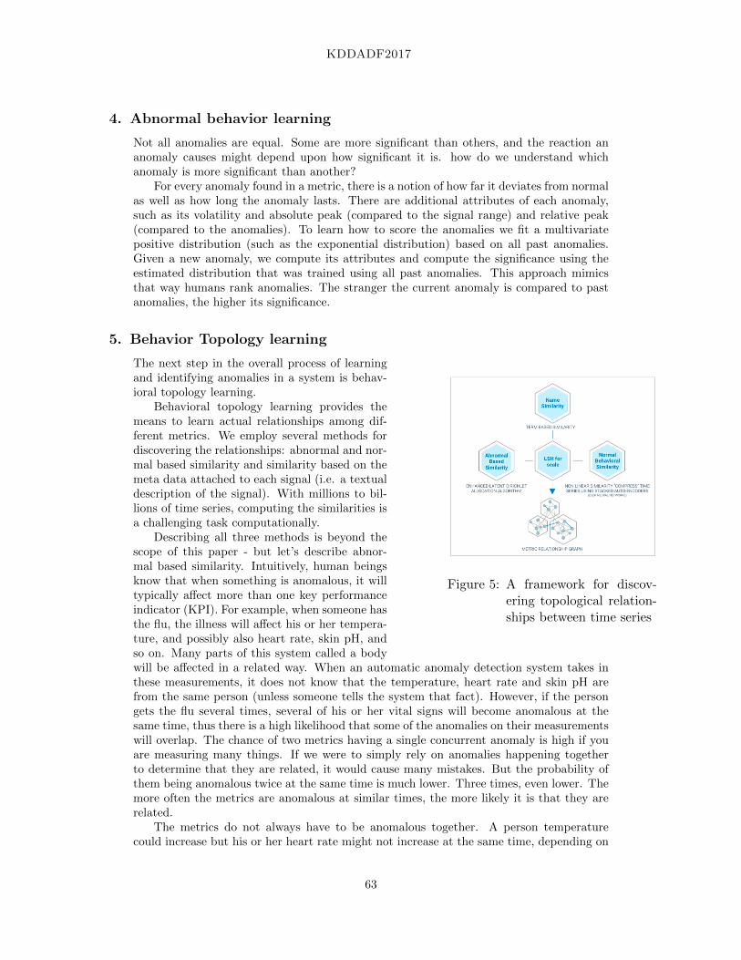
Figure 5: A framework for discov-ering topological relation-ships between time series

The next step in the overall process of learningand identifying anomalies in a system is behav-ioral topology learning.

Behavioral topology learning provides themeans to learn actual relationships among dif-ferent metrics. We employ several methods fordiscovering the relationships: abnormal and nor-mal based similarity and similarity based on themeta data attached to each signal (i.e. a textualdescription of the signal). With millions to bil-lions of time series, computing the similarities isa challenging task computationally.

Describing all three methods is beyond thescope of this paper - but let’s describe abnor-mal based similarity. Intuitively, human beingsknow that when something is anomalous, it willtypically affect more than one key performanceindicator (KPI). For example, when someone hasthe flu, the illness will affect his or her tempera-ture, and possibly also heart rate, skin pH, andso on. Many parts of this system called a bodywill be affected in a related way. When an automatic anomaly detection system takes inthese measurements, it does not know that the temperature, heart rate and skin pH arefrom the same person (unless someone tells the system that fact). However, if the persongets the flu several times, several of his or her vital signs will become anomalous at thesame time, thus there is a high likelihood that some of the anomalies on their measurementswill overlap. The chance of two metrics having a single concurrent anomaly is high if youare measuring many things. If we were to simply rely on anomalies happening togetherto determine that they are related, it would cause many mistakes. But the probability ofthem being anomalous twice at the same time is much lower. Three times, even lower. Themore often the metrics are anomalous at similar times, the more likely it is that they arerelated.

The metrics do not always have to be anomalous together. A person temperaturecould increase but his or her heart rate might not increase at the same time, depending on

63

KDDADF2017

the illness. But we know that many illnesses do cause changes to the vital signs together.Based on these intuitions, one can design algorithms that find the abnormal based similaritybetween metrics. One way to find abnormal based similarity is to apply clustering. Onepossible input to the clustering algorithm would be the representation of each metric asanomalous or not over time (vectors of 0s and 1s); the output is groups of metrics thatare found to belong to the same cluster. While there are a variety of clustering algorithms,“soft” clustering is required in this case, as a metric may belong to multiple groups. LatentDirichlet Allocation is an example algorithm that allows each item (metric) to belong tomultiple groups.

Scaling such methods is also important. Using Locality Sensitive Hashing on the vectorrepresenting each metric provides initial rough grouping of the entire set of metrics, and ineach the full algorithm can be applied.

Figure 5 illustrates the three types of similarities learned to create the behavioraltopology. Once learned, metrics can be grouped to discover complex multivariate anomalies.

6. Results

Example of important anomalies are abundant in our system. Figure 6(a) illustrates ananomaly discovered by our system that is fraud related. A bot begins attempting to searchfor products in multiple zipcodes, causes increase in pageviews, unique zipcode relatedsearches, and bounce rates, while decreasing the average time on page, among other metrics.The anomaly group highlights that it happens on a particular site, with traffic originatingfrom a certain geography and client side operating system. Quickly blocking the bot’sactivity using his signature stops the attack before any damage is done.

Figure 6(b) illustrates the importance of all the steps in an anomaly detection system:normal behavior learning, abnormal behavior learning, and behavioral topology learning.It is based on 4 million metrics for one company over a period of a week. Out of this,we found 158,000 single metric anomalies in a given week, meaning any anomaly on anymetric. This is the result of using our system to do anomaly detection only at the singlemetric level, without anomaly scoring and without metric grouping. Without the meansto filter things, the system gives us all the anomalies, and that is typically a very largenumber. Even though we started with 4 million metrics, 158,000 is still a very big number,too big to effectively investigate; thus, we need the additional techniques to whittle downthat number. If we look at only the anomalies that have a high significance score, in thiscase a score of probability of 0.7 (score 70) or above, the number of anomalies drops offdramatically by an order of magnitude to just over 910. This is the number of significantanomalies we had for single metrics out of 4 million metrics for one week, 910 of them.Better, but still too many to investigate thoroughly. The bottom of the funnel showshow many grouped anomalies with high significance we end up after applying behavioraltopology learning techniques. This is another order of magnitude reduction, from 910 to147. This number of anomalies is far more manageable to investigate. Any organizationwith 4 million metrics is large enough to have numerous people assigned to dig into thedistilled number of anomalies, typically looking at those anomalies that are relevant totheir areas of responsibility.

7. Summary

In this paper we outlined our large scale anomaly detection system, which is used commer-cially by dozens of companies. We described the requirements from such a system and howwe addressed them: namely, advanced algorithms to learn normal behavior, an abnormal

64

KDDADF2017

(a)

(b)

Figure 6: (a) An anomaly which includes multiple metrics (51) showing a bot related fraudon a commercial website. (b) Illustration of the importance of all steps

behavior probabilistic model, and scalable methods for discovering relationships betweentime series for the purpose of anomaly grouping.

To date, our system handled over 120 million time series, discovering around 20 millionwith seasonal patterns, over a 500 million discovered relationships between metrics andprocessing over 6 billion data points per day. We have not discussed the method by whichfeedback from users on the quality of anomalies affect the learning methods - pushing thelearning problem towards a semi-supervised approach, whenever such labels are available.

References

Varun Chandola, Arindam Banerjee, and Vipin Kumar. Anomaly detection: A survey. volume 41,page 15. ACM, 2009.

Chris Chatfield. The holt-winters forecasting procedure. pages 264–279. JSTOR, 1978.

Chris Chatfield. The analysis of time series: an introduction. CRC press, 2016.

Balachander Krishnamurthy, Subhabrata Sen, Yin Zhang, and Yan Chen. Sketch-based changedetection: methods, evaluation, and applications. In Proceedings of the 3rd ACM SIGCOMMconference on Internet measurement, pages 234–247. ACM, 2003.

Vladilen F. Pisarenko. The retrieval of harmonics from a covariance function. volume 33, pages347–366, 1973. URL http://gji.oxfordjournals.org/content/33/3/347.short.

Ralph Schmidt. Multiple emitter location and signal parameter estimation. volume 34, pages 276–280. IEEE, 1986.

Peter Welch. The use of fast fourier transform for the estimation of power spectra: a method basedon time averaging over short, modified periodograms. volume 15, pages 70–73. IEEE, 1967.

65