Real Price and Wage Rigidities in a Model with Matching Frictions∗

Keith Kuester

Goethe University

February 13, 2006

Abstract

I reconcile macro- and micro-evidence on price setting in a search and matching framework.

Search frictions lead price-setting firms to negotiate wage rates with their employees. The in-

crease in strategic complementarity of price-setting leads to substantial real price rigidities which

in turn reduce implied price durations. At the same time this mechanism dampens the reaction

of real wage rates to aggregate fluctuations which is necessary to explain the highly volatile

response of vacancies in the data. A further interesting finding is that inflation via the Phillips

curve is not only driven by an output gap but also by an employment gap – a feature usually

neglected in empirical research. I demonstrate that the modified model can be parameterized

such that it can replicate impulse responses to monetary policy shocks obtained from a struc-

tural VAR for post Volcker-disinflation U.S. data.

JEL Classification System: E31,E24,E32,J63,J64

Keywords: firm-specific labor, real rigidities, Phillips curve, wage rigidity, bargaining.

∗ Correspondence: Goethe University, Postbox 94, 60325 Frankfurt am Main, Germany, Tel.: +49 69 798-25285,Fax: +49 69 798-25272, e-mail: kuester@wiwi.uni-frankfurt.de.

I am indebted to my colleague Gernot Mueller for providing his impulse response matching code and for manyhelpful comments. Without implicating, I would also like to thank Philip Jung, Michael Krause and Dirk Kruegerfor valuable comments.

1 Introduction

The microfoundations paradigm, which nowadays is at the forefront of macroeconomic thinking,

aims at bringing macroeconomics in line with microeconomic theory and evidence. In this

respect, one apparent failure of recent estimates of plain Calvo-type Phillips curves for the U.S.

is that these imply that firms change their prices only every six quarters – or even less often

(see Gali and Gertler, 1999, Eichenbaum and Fisher, 2004). Micro-level evidence, however,

shows that U.S. firms on average adjust much more often: at least every second quarter (see

Bils and Klenow, 2004, and Klenow and Kryvtsov, 2005).1

Real price rigidities help to reconcile micro- and macro-evidence (see e.g. Ball and Romer, 1990,

Altig, Christiano, Eichenbaum, and Linde, 2005, and Woodford, 2003, chapter 3). If average

price changes are small, price changes can be frequent while still being consistent with a smooth

inflation series. This paper stresses that the search and matching model (e.g. Pissarides, 1985)

is a natural candidate to generate these real price rigidities.2

In the search and matching model labor is a temporarily firm-specific factor of production, i.e. the

firm cannot hire labor in a competitive market. To the contrary, frictions when searching for a

new worker lead a firm to share rents with its employee via wage bargaining. Considering a firm

that contemplates raising its price, lower demand due to a higher sales price translates into less

hours worked and hence a fall in the worker’s marginal disutility of work. The standard Calvo

model features constant marginal costs of production. In the search and matching framework,

in contrast, the associated decrease in the worker’s subjective wage rate (his marginal rate

of substitution between leisure and consumption) translates into lower marginal costs for the

firm. This fall in marginal costs in turn depresses the incentive to raise the price in the first

place. Compared to the standard Calvo model with constant marginal costs, in the framework

advocated in this paper firms will therefore opt for smaller price changes.

The technical contribution of the current paper is to directly integrate the wage bargaining into

a sector which produces differentiated goods and hence has a margin for setting its price but

1 This contradiction qualitatively is not confined to the U.S.. For the Euro area as a whole, Dhyne, Alvarez,Bihan, Veronese, Dias, Hoffman, Jonker, Lunnemann, Rumler, and Vilmunen (2005) examine consumer pricedata. They stress that price spells last on average between 4 and 5 quarters and that the median durationis 3 to 4 quarters. While this micro-level duration is larger than for the US it is still in stark constrastto the macro-level estimates in Smets and Wouters (2003), say, which imply that prices change every 9-10quarters only. Similar evidence can be foud in Gali, Gertler, and Lopez-Salido (2001) when one abstractsfrom features which make marginal cost responsive to own output. Interestingly, previous stylized facts forthe U.S. concluded that prices were substantially more sticky. The survey by Taylor, 1999, e.g., concludedthey were constant for slightly less than a year.

2 Christiano, Eichenbaum, and Evans (2005) emphasize three other channels which tend to induce a smallinflation response: variable capital utilisation, sticky wages and working capital. The latter channel works inthe event of a monetary easing. If firms have to borrow their wage bill, a fall in the nominal interest rate willreduce their interest burden and thus marginal cost. This has a dampening effect on inflation or can even leadto an initial fall.

1

to retain ex-ante worker homogeneity (as a counterexample, see e.g. Trigari, 2004 and Braun,

2005, for the “standard” new Keynesian implementation of the search and matching model with

constant marginal cost).3

Pointing to the importance of firm-specific factors in reconciling the macro and micro-evidence

on price setting has some tradition in the literature. While firm-specific labor has been explored

to a lesser extent, the potential importance of firm-specificity of capital has recently been met

by considerable interest; see Sbordone (2002), Woodford (2003, 2004), Sveen and Weinke (2004),

Christiano (2004), Eichenbaum and Fisher (2004) and Altig, Christiano, Eichenbaum, and Linde

(2005). Another way to reconcile Phillips curve estimates with micro-evidence is to assume

decreasing returns to factors of production, see e.g. Gali, Gertler, and Lopez-Salido (2001), or

to assume a non-constant elasticity of demand (a slightly kinked demand curve), which makes it

easier to loose customers by raising a firm’s price than to gain customers by lowering it, i.e. the

elasticity of demand is falling sharply with a firm’s market share (hence rising sharply in a firm’s

price) see Kimball (1995).4

Closest to the current paper is Woodford (2003, ch. 3). He has explored real rigidities originating

from the labor choice. In his model there are different types of labor. Each type of labor is used

to produce a specific variety of a differentiated good. The marginal cost of production increases

in output due to an increase in the marginal rate of substitution between leisure and labor on

the worker side, similar to the mechanism in my paper. Woodford needs to make the strong

assumption that labor is completetely firm-specific and worthless outside of the specific firm.5

In my model, in contrast, the firm-specific factor is only firm-specific as long as the match is not

severed, i.e. there is an outside market value to the worker. Costly search and matching creates

a quasi-rent for existing jobs that can be shared between firm and worker via a wage payment.

Wage rates in turn determine the magnitude of the response of firms’ profits to aggregate

shocks and hence vacancy posting and the creation of employment relationships.6 Hall (2005)

and Shimer (2004) argue that the Mortensen and Pissarides (1994) model’s shortcomings in

accounting for the sizeable reaction of vacancies (and thus market tightness, the Beveridge curve)

to reasonably sized shocks can be attributed to the standard assumption of wage determination

3 An exception to the standard modeling scheme is Krause and Lubik (2006) who assume that wage bargainingand price-setting takes place in the same sector (they assume quadratic price adjustment costs). Krause undLubik, however, assume that utility is linear in hours worked. With this assumption, the marginal rate ofsubstitution does not change in hours worked and thus, there are no real price rigidities. In addition, they donot derive a model-consistent wage rigidity.

4 Similar effects arise when consumption habits are product specific. This also leads to pro-cyclical own priceelasticities of demand; see Ravn, Schmitt-Grohe, and Uribe (2006).

5 A similar assumption in a firm-specific capital environment is found in Altig, Christiano, Eichenbaum, andLinde (2005).

6 Note that in contrast to Hall (2005) wage rates are allocational even for existing matches since hours workedare an endogenous variable in my model.

2

via Nash-Bargaining. For a critical appraisal of this literature see Mortensen and Nagypal

(2005). Besides reconciling micro- and macro-evidence on price setting, my model provides for

significant real wage rigidity, a fact Hall (2005) and Shimer (2004) argue is important to match

labor market fluctuations. In particular, an increase in strategic complementarity in price-setting

translates into more rigid real wages.7

As to the results, I find that the raised degree of strategic complementarity in price-setting not

only dampens the response of inflation to aggregate shocks but also induces the real wage rate to

be less volatile. The smooth wage rate series implied by the model in turn helps to replicate the

fluctuation of vacancies found in U.S. data. An interesting finding of my paper is furthermore

that the Phillips curve once accounting for variations on the extensive margin of employment

is not only driven by the output gap, as is commonly assumed in the empirical literature, but

also by an “employment gap”. Omitting the latter (as most of the literature does) is likely to

bias implied price-durations inferred from Phillips curve estimates upwards – and thus is likely

to bias estimates for the price duration against the micro-evidence.

The next section lays out the model. Section 3 discusses some of the (linearized) equilibrium

conditions. Special emphasis is on the implied reduced form Phillips curve. The fit of the

Phillips curve hinges critically on the value of the own-prive elasticity of demand. A change

in the elasticity, however, also directly affects the transmission in the labor market. In section

4 I therefore illustrate that the entire model can replicate the impulse responses to monetary

policy shocks taken from a small structural vector autoregression. A final section wraps up and

concludes. Some technical material and a thorough description of the data is deferred to the

Appendix.8

2 The Model

According to Hall (2005) the separation rate does not vary much over the U.S. business cycle.

Cyclical fluctuations in employment are mainly due to fluctuations in vacancy posting – I there-

fore do not model endogenous separation in this paper but assume that each period a constant

fraction of firm-worker relationships splits up for reasons exogenous to the state of the economy.

As is common in the literature, I focus on a cashless limit economy; cp. Smets and Wouters

(2003) and large parts of Woodford (2003).

7 The mechanism therefore differs from Gertler and Trigari (2005) who use staggered Calvo wage-setting in areal-business cycle model. Since in their setup, it is not clear how, if wages are left unchanged, hours aredetermined, they have to shut-down the intensive margin completely. In my model, the assumption of wageand pricing setting being conducted in the same sector, leads hours worked to be (demand-)determined. Also,Gertler and Trigari (2005) lack the amplification mechanism for wage rigidity, which I discussed above.

8 A further technical appendix which derives the model equations in linearized form is available from the authorupon request.

3

2.1 Consumers

The model economy consists of a large number of identical families. Each family has a continuum

of members of two types: unemployed workers with mass ut and employed workers with mass

nt. The total mass of workers and families each is normalized to one. Families earn real income

from the real wages of their employed members, ntwtht, where wt is the real wage rate per

hour worked, ht. They, in addition, obtain income from real unemployment benefits, b, which

unemployed members receive (utb in total) and from holding pure discount bonds. Families

also hold shares in a mutual fund that redistributes profits in the economy. Family members,

indexed by i, are infinitely lived and seek to maximize expected lifetime utility by deciding on

the level (and intertemporal distribution) of consumption of a bundle of consumption goods, cit,

and by deciding on the real expenditure, dit, for riskless one-period bonds:

max{ci

t,dit}Et

∞∑

j=0

βj{U(cit+j , ct+j−1) − g(hi

t+j)} , β ∈ (0, 1). (1)

Household members pool their income – there is thus perfect consumption risk sharing. We

assume that households take the labor supply decision for their members in order to prevent

free-riding. The family member’s budget constraint is given by:

utb+ ntwtht +di

t−1

ΠtRt−1 +

∫ nt

0ψj

t dj = cit + dit + tt + vtκt. (2)

Here Rt denotes the nominal gross return on the bond from t to t + 1 and Πt is the gross

consumer price inflation rate. The wholesale sector firms’ profits, ψjt , accrue to the households,∫ nt

0 ψjt dj. vt are the number of vacancies, κt are real costs of posting a vacancy. Vacancy posting

costs are assumed to be lump-sum tax costs. They thus enter the household’s budget constraint

but not the aggregate ressource constraint. The household pays lump-sum taxes tt.

Let ct−1 be the aggregate level of consumption in period t − 1. I assume that an individual’s

consumption is subject to external habit persistence, indexed by parameter hc ∈ [0, 1),

U(cit, ct−1) =(cit − hcct−1)

1−σ

1 − σ, σ > 0. (3)

As in Abel (1990) households therefore are concerned with “catching up with the Joneses”.

The first-order conditions for consumption versus saving can be summarized by the Euler equa-

tion

λt = βEt

{λt+1

Rt

Πt+1

}, (4)

where λt = (ct − hc ct−1)−σ marks marginal utility of consumption.9 The optimal consumption

9 Due to consumption insurance and separability of consumption and leisure in the utility function, all households

4

plan in equilibrium also satisfies the merged transversality and no-Ponzi condition

lims→∞

Et

{βsλt+s

λtdt+s

}= 0. (5)

Completing the description of preferences, disutility of work is characterized by

gt(hit) = κh

ht(i)1+φ

1 + φ, φ > 0, κh > 0. (6)

Here, κh denotes a scaling parameter for the disutility of work. Importantly for the argument

below, the marginal disutility of work, ∂g(h)∂h

, is increasing in individual hours worked, hit. It is

this fact which leads a worker to seek increasing compensation per hour on the margin (due to

an increase in his subjective price of work). This in turn induces firms to adjust prices (and,

implicitly, their demand-driven output) by less than in the standard model.

2.2 Production

The existing macro-labor market literature assumes that firms which are free to set prices face

constant marginal cost; e.g. Trigari (2004), Braun (2005) and Christoffel, Kuester, and Linzert

(2005) assume that labor is used only as an input into an intermediate good. This in turn is

sold to a differentiating sector in perfectly competitive markets. The major contribution of the

current paper is to integrate the labor market activity into the price setting sector, i.e. to let

firms which are free to set their price also negotiate wages. Again, it is this change combined

with the increasing marginal disutility of work that allows to bring about the real price (and

ultimately wage) rigidity.

There are two types of firms. Firms in the wholesale sector need one worker to produce. Whole-

sale firms which have a worker produce differentiated goods which they sell under monopolistic

competition. They are subjected to time-dependent price (and wage) setting impediments a la

Calvo (1983).10 Firms and workers, if they are allowed to update, decide jointly how to split the

rents of their employment relationship. Hours worked are demand-driven (hence dependent on

the firm’s sales price) and have a first-order effect on individual utility. I therefore assume that

a firm and a worker not only decide about the nominal hourly wage rate, W jt , but that they

simultaneously also bilaterally agree on the product price, P jt – again, since the price determines

in equilibrium will have the same consumption levels. I therefore suppress index i here.

10 Klenow and Kryvtsov (2005) summarize that individual price data obtained from the U.S. Bureau of LaborStatistics reveal that (a) price changes are largely non-synchronized, (b) variation in the magnitude of pricechanges contributes much more to the variation in aggregate inflation (90+%) than variation in the number

of price changes and (c) the size of absolute price changes is large, over 8%. Overall they conclude that theDotsey, King, and Wolman (1999) state-dependent pricing model, once calibrated to match the micro-pricedata, very much resembles the Calvo-model in so far as pricing behavior is concerned. Modeling pricing astime-dependent may thus not be an overly stringent assumption.

5

hours worked via the firm’s demand function.A greatly simplifying assumption is that wages and

prices have the same duration: whenever a firm resets its price it renegotiates its wage and vice

versa.11 Retailers bundle the differentiated goods and sell the homogenous consumption basket

yt at price Pt.

2.2.1 Retail Firms

Let nt ∈ (0, 1) be employment in t. Since workers are employed in one-worker wholesale firms

this means that nt wholesale firms engage in production. Thus a total mass of nt varieties

yjt , j ∈ [0, nt], of wholesale goods is produced in a given period. Retail firms in turn operate

in perfectly competitive product markets. They buy differentiated wholesale goods, yt(j), and

produce yt units of the consumption good according to

yt = nt

[1

nt

∫ nt

0yt(j)

ǫ−1ǫ dj

] ǫǫ−1

. (7)

The cost-minimizing demand for wholesale goods of type j is

yjt =

(P j

t

Pt

)−ǫ

yat , (8)

where yat marks average output per employed worker, ya

t = 1ntyt, and ǫ > 1 is the own-price

elasticity of demand. The consumption good price index Pt is given by

Pt =

[1

nt

∫ nt

0Pt(j)

1−ǫdj

] 11−ǫ

. (9)

2.2.2 Wholesale Firms

There is an infinite number of potential one-worker wholesale good producers. Wholesale firms

engage in vacancy posting. Once having recruited a worker, they produce a differentiated good

and engage in wage bargaining. I describe each decision in turn.

11 After all, this assumption may not be as stringent as it seems: In their benchmark version estimated onaggregate U.S. data, Christiano, Eichenbaum, and Evans (2005) find that prices and wages roughly have thesame duration, 2.5 and 2.8 quarters, respectively. Crucial for their estimates in line with micro-evidence is theassumption of working capital and variable capital utilization, features which I do not have in my model. Alsoon aggregate data, in contrast, Altig, Christiano, Eichenbaum, and Linde (2005) find that wages are changedless frequently: every 3.6 quarters. Direct evidence for wage rigidity is scarcer: there is no systematic directevidence on the frequency of wage negotiations. In a survey Taylor (1999) argues that wages are typicallyadjusted once per year. Based on micro-level data on wages per hour, Gottschalk (2004) concludes similarly.Yet this evidence applies mainly to base pay. Other wage components like bonuses or perks will likely adjustmore frequently.

6

Vacancy Posting. Firms without a worker have to incur a real vacancy posting cost, κt > 0,

in order to stand a chance of recruiting a worker. The model allows for fluctuations in vacancy

posting costs, e.g. since there are vacancy adjustment costs as in Braun (2005) or because

vacancy costs are posted in nominal terms.12 Vt is the market value of a prototypical firm that

posts a vacancy in period t. Jt(Pjt ,W

jt ) is the value of a wholesale firm in period t that has a

worker, charges P jt for its good and pays W j

t for each hour worked. Due to nominal rigidities,

each period workers and firms can renegotiate prices and wages only with probability 1 − ϕ.

Otherwise they partially update (but do not reoptimize) their price and wage by the realized

gross inflation rate (Πγp

t−1 and Πγw

t−1, respectively, γp, γw ∈ [0, 1]).13 For analytical tractability,

I keep the heterogeneity to a minimum by assuming that firms which just found a worker,

i.e. enter the market, have the same pricing pattern as existing firm-worker relationships:14

They can choose their optimal price, P ∗

t , and their optimal wage rate, W ∗

t , (both to be defined

below) with probability 1 − ϕ. With probability ϕ, however, they have to set previous period’s

average price and wage (suitably indexed). A firm which posts a vacancy finds a new employee

with probability qt. With probability ρ this new match is severed for an exogenous reason prior

to production in t. Firms which loose their worker cease to exist and are therefore worthless.

The value of a firm which opened a vacancy consequently is given by

Vt = −κt + qt(1 − ρ)Et

{βt,t+1

[ϕJt+1(Pt Π

γp

t ,Wt Πγw

t ) + (1 − ϕ)Jt+1(P∗

t+1,W∗

t+1)]}. (10)

Here βt,t+1 := β λt+1

λtis the equilibrium pricing kernel. There is free entry into production apart

from the sunk vacancy posting cost. This drives the value of a vacancy to zero in equilibrium:

Vt!= 0.

Production. Each wholesale firm has the same linear production technology

yjt = zth

jt . (11)

zt marks the economy-wide level of labor productivity.

A firm in production makes a real profit ψt in period t, which depends on the wage rate paid to

12 The empirical exercise in Section 4 shows that constant vacancy posting costs, i.e. κt = κ ∀ t, are sufficient tofit the vacancy series .

13 The partial updating follows Christiano, Eichenbaum, and Evans (2005) and Smets and Wouters (2003).

14 In addition, to achieve sufficient fluctuation in vacancies, Shimer (2004) argues that real wages of newly formedmatches must be sticky in order to induce sufficient fluctuation in vacancies and unemployment – a fact, thatis achieved by my formulation.

7

its employee and the price charged for its product:

ψt

(P j

t ,Wjt

)=P j

t

Ptyj

t −W j

t

Pthj

t . (12)

With probability 1−ρ the current match will not be severed at the beginning of the next period.

Conditional on survival, with probability ϕ the firm has to retain its current price and wage.

With probability 1−ϕ, however, it can set the new optimal price-wage pair, P ∗

t+1,W∗

t+1. Whence

the value of one of the nt firms which produce in t is

Jt

(P j

t ,Wjt

)= ψt(P

jt ,W

jt )

+(1 − ρ)Et

{βt,t+1

[ϕJt+1

(P j

t Πγp

t ,Wjt Πγw

t

)+ (1 − ϕ)Jt+1

(P ∗

t+1,W∗

t+1

)]}.

(13)

Matching. I assume a constant-returns to scale matching function, linking new matches, mt,

to unemployment, ut, and vacancies, vt:

mt = σmuαt v

1−αt , σm > 0, α ∈ [0, 1]. (14)

σm governs the rate at which new matches arrive, the efficiency of matching. α governs the

relative weight the pool of searching workers and firms, respectively, receive in the matching

process. Define labor market tightness (from the view point of a firm) as θt := vt/ut. The

probability that a vacant job will be filled is qt = mt/vt. The probability that an unemployed

worker finds employment is st = mt/ut. Workers which are matched to a firm in t will not start

working before t+ 1. Employment therefore evolves according to

nt = (1 − ρ)(nt−1 +mt−1). (15)

Unemployment is

ut = 1 − nt. (16)

Worker Surplus. An employed worker receives his real wage bill and suffers disutility of work,g(hj

t )λt

, where λt is the marginal utility of consumption. Next period he remains employed with

probability 1 − ρ or will be unemployed otherwise (ρ). The value of employment, Γt(·), to the

8

worker who is employed in a firm with price P jt and wage rate W j

t is

Γt(Pjt ,W

jt ) =

W jt

Ptht(P

jt ) −

gt

(ht(P

jt ))

λt

+ (1 − ρ)ϕEt

{βt,t+1Γt+1(P

jt Π

γp

t ,Wjt Πγw

t )}

+ (1 − ρ)(1 − ϕ)Et

{βt,t+1Γt+1(P

∗

t+1,W∗

t+1)}

+ ρEt {βt,t+1Ut+1} .

(17)

Note that the value of employment next period again depends on the price-wage stickiness.

Similarly the value of a worker who is unemployed during t is

Ut = b

+ st(1 − ρ)ϕEt

{βt,t+1Γt+1(PtΠ

γp

t ,WtΠγw

t )}

+ st(1 − ρ)(1 − ϕ)Et

{βt,t+1Γt+1(P

∗

t+1,W∗

t+1)}

+ (1 − st + stρ)Et {βt,t+1Ut+1} .

(18)

Above, b are real unemployment benefits. The worker’s surplus from being in employment,

i.e. the increase of family utility through an additional family member in employment in t is

∆t(Pjt ,W

jt ) := Γt(P

jt ,W

jt ) − Ut.

15 Hence

∆t(Pjt ,W

jt ) =

W jt

Ptht(P

jt ) −

gt

(ht(P

jt ))

λt− b

+ (1 − ρ)ϕEt

{βt,t+1(∆t+1(P

jt Π

γp

t ,Wjt Πγw

t ) − ∆∗

t+1)}

− (1 − ρ)ϕstEt

{βt,t+1(∆t+1(PtΠ

γp

t ,WtΠγw

t ) − ∆∗

t+1)}

+ (1 − ρ)(1 − st)Et

{βt,t+1∆

∗

t+1

},

(19)

where ∆∗

t+1 = ∆t+1(P∗

t+1,W∗

t+1).

Bargaining. Wholesale firm-worker pairs which are allowed to update their price and wage

in period t face the problem of maximizing joint surplus by choosing the sales price and by

simultaneously negotiating the nominal wage rate. This specification has the advantage that

while wages and prices may be fixed, hours worked can freely adjust to satisfy demand. I stick

15 This can be derived from first principles by assuming that workers value their labor-market actions in termsof the contribution these actions give to the utility of the family to which they belong and with which theypool their income; see Trigari (2004).

9

to the Nash-bargaining assumption: Firms and workers solve

maxW

jt ,P

jt

[∆t(P

jt ,W

jt )]η [

Jt(Pjt ,W

jt )]1−η

, (20)

where η ∈ (0, 1) is the worker’s bargaining power.

While not born out by the simple notation, the bargaining problem is not a trivial one: the

firm and the worker need to take into account the effect of their decision today on all periods in

which they may have to keep prices and wages fixed.16 Let P ∗

t and W ∗

t denote the optimal price

and wage, respectively. Define J∗

t := Jt(P∗

t ,W∗

t ). The first-order condition for price setting is

∂∆t(Pjt ,W

jt )

∂P jt

∣∣∣∣∣(P j

t ,Wjt )=(P ∗

t ,W ∗

t )

ηJ∗

t = −∂Jt(P

jt ,W

jt )

∂P jt

∣∣∣∣∣P ∗

t ,W ∗

t

(1 − η)∆∗

t . (21)

The first-order condition for optimal wage setting is

∂∆t(Pjt ,W

jt )

∂W jt

∣∣∣∣∣P ∗

t ,W ∗

t

ηJ∗

t = −∂Jt(P

jt ,W

jt )

∂W jt

∣∣∣∣∣P ∗

t ,W ∗

t

(1 − η)∆∗

t . (22)

The fact that wages and prices are always set at the same time greatly simplifies the derivation

of a linearized version of the model since it keeps heterogeneity among firms and workers,

respectively, within manageable bounds.

2.3 Government

2.3.1 Monetary Policy

The monetary authority is assumed to control the nominal one-period risk-free interest rate,

Rt. In the following, let hats over variables denote percentage deviations of these variables from

steady state. The empirical literature (see, e.g. Clarida, Gali, and Gertler, 1998) finds that

simple linearized generalized Taylor-type rules of the form

Rt = ρmRt−1 + (1 − ρm)γπEtπat+3 + (1 − ρm)γyyt + ǫ money

t (23)

are a good representation of monetary policy. Here ρ ∈ [0, 1), γπ > 1, γy ≥ 0 and ǫmoneyt is

an iid shock. The use of specific inflation rate concept differs in these rules. I assume that the

policymaker targets average annual inflation, πat+3 := 1

4 (πt + πt+1 + πt+2 + πt+3) .17

16 A technical appendix which goes more in depth with the derivations is available from the author.

17 Such a policy rule can be rationalized by the following rule in levels:

Rt = (Π/β)1−ρRρt−1Et

�Πa

t+3

Π

�(1−ρ)γπ�yt

y

�(1−ρ)γy

ǫmoneyt . (24)

10

2.3.2 Fiscal Policy

I assume that fiscal policy is Ricardian. The government does not engage in any government

spending. It redistributes any income from debt issues and vacancy posting taxes to the private

agents via lump-sum transfers (−tt) and unemployment benefits. The government’s budget

constraint is:

utb+dt−1

ΠtRt−1 = dt + tt + vtκt. (25)

Since the path of debt is not the focus of the current paper, an arbitrary debt-stabilizing rule

will close the government sector.

2.4 Market Clearing

Market clearing in the market for wholesale and final retail goods requires

yt = ct, (26)

where

yt = nt

[1

nt

∫ nt

0yt(j)

ǫ−1ǫ dj

] ǫǫ−1

, ǫ > 1. (27)

Here yjt =

(P

jt

Pt

)−ǫ

yat = zth

jt . In addition, the market for government bonds needs to clear.

3 Intuition from the Linearized Model

To repeat the focus of the paper: the New-Keynesian labor-market literature so far parts wage

bargaining from price setting. This assumption causes marginal cost in the monopolistically

competitive sector to be independent of own production, see e.g. Trigari (2004). I call this the

“standard” world. The contribution of the current paper is to bring the firm-specifity of labor

in the bargaining world to the forefront. I show that this specification is simple enough (once

linearized) to be amenable to empirical research and derive implications for estimates of new

Keynesian Phillips curves.

In passing, I provide a means to incorporate real wage rigidity, a fact that Hall (2005) and

Shimer (2004) argue might be necessary to fit the fluctuations of vacancies. The degree of real

wage rigidity in my model itself intensifies when the degree of strategic complementarity in price-

setting increase.18 Below, I present part of the model after linearizing around the zero-inflation

steady state laid out in Appendix A.19 After some manipulation, the Phillips curve (πt is the

Here Π is the target for the quarterly gross inflation rate in steady state (which equals steady state inflation)and y is steady state potential output.

18 This amplification mechanism is absent in the work of Gertler and Trigari (2005).

11

deviation of the inflation rate from its steady state) can be reduced to

πt =γp

1 + γp βπt−1 +

β

1 + γp βEtπt+1 +

1 − ϕ

ϕ

1 − β ϕ

1 + γp βdt, (28)

where

dt =1

1 + φǫ{mrst − zt} .

Here β = β(1 − ρ) and mrst is the average marginal rate of substitution between leisure and

consumption of employed workers.

Define the natural rate of average output under flexible prices as ya,nt and the natural marginal

utility of consumption under flexible prices as λnt . With these definitions the term dt in the

Phillips curve (28) can be written as:

dt =1

1 + φǫ

{φ (ya

t − ya,nt ) − (λt − λn

t )}. (29)

The marginal utility of consumption, λt, in turn depends on total output, not on average output.

This means that once substituting for marginal utility of consumption, an employment gap enters

the Phillips curve:

dt =1

1 + φǫ

{φ [yt − yn

t − (nt − nnt )] +

σ

1 − hc

[yt − yn

t − hc

(yt−1 − yn

t−1

)]}

=1

1 + φǫ

{φ [ygap

t − ngapt ] +

σ

1 − hc

[ygap

t − hcygapt−1

]}.

(30)

The Phillips curve looks very similar to Woodford (2003, p. 187) and Boivin and Giannoni

(2006) – without the need to assume any ex ante worker heterogeneity. Instead, the matching

model naturally lends itself to an increase of the strategic complementarity of price-setting

decisions due to firm-specific labor. Comparing (28) and (30) to the standard New Keynesian

Phillips curve (e.g. Gali and Gertler, 1999), which is obtained as the special case φ = 0, ρ = 0,

three differences stand out. First, in the matching model the firm implicitly discounts the

future more intensively owing to its lower survival probability. And indeed, estimates of new

Keynesian Phillips curves for the US and other economies consistently show that the reduced

form discount factor is estimated to be significantly well below unity, see e.g. Gali and Gertler

(1999), Gali, Gertler, and Lopez-Salido (2001) and Gagnon and Khan (2005). Second, for

reasonable parameter values the factorφ+ σ

1−hc

1+φǫis smaller than unity, implying more strategic

complementarity in price setting. The degree of strategic complementarity rises as the elasticity

of demand increases which substantially dampens the effect of aggregate shocks on inflation

19 The derivation is explained in detail in a technical appendix available from the author upon request.

12

as illustrated in Woodford (2003).20 Similar multiplicative factors are found in the existing

real rigidities literature (e.g. Altig et al., 2005; Eichenbaum and Fisher, 2004). Third, the

employment gap enters as an additional regressor. Since output is positively correlated with

employment in the data, according to this model even reduced form estimates of the slope of

the Phillips curve, when they omit the employment gap, may be biased downwards (implying

price durations which are biased upwards).21

In my model, also two other optimality conditions are altered. Vacancy posting is affected by

the gap between the optimal wage and the average wage rate.22 In addition the law of motion

for aggregate wages is changed, to which I turn next.

While the wage equation looks somewhat inaccessible in general, intution can be gained by

restricting the analysis to the case w = mrs in steady state.23

20 Usually, the elasticity of demand, ǫ is calibrated to be much larger than unity. Woodford (2003) uses a valueof 7.6, Altig, Christiano, Eichenbaum, and Linde (2005) use a value of 101.

21 Preliminary examination showed that this will, however, not solve the problems in Gali and Gertler (1999)when using conventional output gap measures to estimate the Phillips curve.

22 The vacancy posting equation can be expressed asbqt = bκt + bλt − [1 − (1 − ρ)β]Etbλt+1 − (1 − ρ)βEt{bκt+1 + bλt+1 − bqt+1}

− [1 − (1 − ρ)β]Etbψ∗

t+1

−ϕ

J

1

1 − βyahǫ�1 −

w e

z

�− 1

iEt {(1 − (1 − ρ)β)bp∗t+1 + bπt+1 − γpbπt}

−ϕ

J

1

1 − βyaw e

zEt { bwt+1 − bwt + bπt+1 − γwbπt − {1 − (1 − ρ)β} [ bwt+1 − bw∗

t+1]} .

(31)

and simplified further to yieldbqt =bκt + bλt − [1 − (1 − ρ)β]Etbλt+1 − (1 − ρ)βEt{bκt+1 + bλt+1 − bqt+1}

− [1 − (1 − ρ)β]Et

�byat+1 −

ew

z − ew( bwt+1 − bzt+1)

�.

23 This exercise is meant to build intuition. Neither do any other relations presented so far depend on thisassumption nor is this condition imposed in the empirical analysis in Section 4.

13

Let wt be the linearized aggregate real wage index. This evolves according to24

α1wt = α2 (wt−1 − πt + γwπt−1)

+ α3Et (wt+1 + πt+1 − γwπt)

+ α4

(θt + κt

)

+ α5

(−λt

)

+ yat

+ (ǫ− 1)zt

(32)

The qualitative features of the wage equation are similar to the standard model: real wages

increase in aggregate output, technology and the marginal rate of substitution. Furthermore,

real wages increase in market tightness and vacancy posting costs.

An additional mechanism in this equation is that real wages are subject to smoothing. Once one

accepts the staggering of the wage and price-setting decisions, this was derived in a completely

model-consistent manner without resorting to social norms or the like. On top, equation (32)

shows a further advantage of this setup a usually free parameter in the Phillips curve has to obey

cross-equation restrictions: the elasticity of demand, ǫ. In fact, the same elasticity of demand, ǫ,

that governs the degree of strategic complementarity in price-setting also has a strong bearing

on the wage-setting process. In general, the larger ǫ the more important the smoothing terms

α2 and α3 in the linearized wage equation (32) become relative to the impact of average output,

market tightness and technology shocks, i.e. the more rigid will be the real wage rate.

4 Empirical Exercise

As mentioned in Section 3 the mechanism of firm-specific labor does not only feature in the

Phillips curve but also elsewhere in the model. I therefore turn to conducting an empirical

exercise to examine the fit of the modified model as a whole. In doing so, I match the DSGE

model’s impulse-responses to monetary policy shocks as closely as possible to the responses ob-

tained in a structural vector-autoregression (SVAR). This exercise is partial in the sense that

I abstract from identifying any aggregate shocks in the economy apart from monetary policy

shocks. The identification assumption in the VAR is standard: apart from Rt non of the observ-

able variables (yt, πt, ht+ nt,vt, ut and wt) react to a monetary policy shock in the same quarter.

Modified Timing Assumptions. The model presented above needs to be slightly modified in

24 All the coefficients are strictly positive. α2 = 1η

ǫ−11−ϕ

ϕ

1−β(1−ρ)ϕ, α1 = α2

1+β(1−ρ)ϕ(ϕ−s)ϕ

, α3 = α2β(1−ρ)(1−s),

α4 = β(1−ρ)s1−β(1−ρ)

, α5 = 1−η

ηǫ−11+φ

.

14

order to reflect the identification assumption in the SVAR. The timing assumption is as follows:

first firms and workers happen to see whether a match is separated. They also see whether they

are allowed to update their price and wage. With this knowledge in mind they take consumption,

price- and wage-setting and vacancy posting decisions. All this information is contained in the

t − 1 information set. The monetary policy shock materializes thereafter at the beginning of

period t. The savings decision is taken with full information. These assumptions leave the Euler

equation (4) unchanged, but consumption is now predetermined:

Et−1λt = (ct − hc ct−1)−σ. (33)

Vacancy posting is also predetermined, so in equilibrium

Et−1Vt = 0. (34)

The price and wage-setting problem alters to

maxW

jt ,P

jt

Et−1

{[∆t(P

jt ,W

jt )]η [

Jt(Pjt ,W

jt )]1−η

}. (35)

The corresponding first-order condition for price setting consequently is

Et−1

{∂∆t(P

jt ,W

jt )

∂P jt

∣∣∣∣∣∗

η∆∗

tη−1J∗

t1−η

}= −Et−1

{∂Jt(P

jt ,W

jt )

∂P jt

∣∣∣∣∣∗

(1 − η)∆∗

tηJ∗

t−η

}, (36)

while the first-order condition for wage-setting as a consequence changes to

Et−1

{∂∆t(P

jt ,W

jt )

∂W jt

∣∣∣∣∣∗

η∆∗

tη−1J∗

t1−η

}= −Et−1

{∂Jt(P

jt ,W

jt )

∂W jt

∣∣∣∣∣∗

(1 − η)∆∗

tηJ∗

t−η

}. (37)

The remainder of the model stays unchanged. I turn to describe the estimation procedure.

The Estimation Procedure. The limited-information procedure I use has been intensively

employed in the literature; see Rotemberg and Woodford (1997), Amato and Laubach (2003),

Boivin and Giannoni (2006), Christiano, Eichenbaum, and Evans (2005) and Meier and Mueller

(2006). For a recent theoretical treatment of “semi-parametric indirect inference” see Dridi,

Guay, and Renault (2006). The econometric methodology consists of selecting the structural

parameters that minimize the distance between the impulse responses of an SVAR to a mon-

etary policy shock and those implied by the model. I thus focus on a subset of the data’s

properties which has been extensively studied and the characteristics of which are relatively

well-established. This simplifies comparability with the literature and – to the extent that the

small model is unable to explain all the features of the data – robustifies the analysis. Formally,

15

let Ψ be the stacked impulse responses obtained from the SVAR and let Ψ(θ) be the impulse

responses of the model evaluated at structural parameters θ which belong to parameter space

Θ. The estimator of the structural parameters is

θ = arg minθ∈Θ

(Ψ − Ψ(θ)

)′

WT

(Ψ − Ψ(θ)

), (38)

where WT is a diagonal weighting matrix involving the inverse of each impulse response’s vari-

ance on the main diagonal as in Christiano, Eichenbaum, and Evans (2005).25 So more weight

is attributed to the responses which are estimated precisely.

Implementation. I estimate a VAR from 1984q1, which marks the end of the non-borrowed

reserves targeting period by the Federal Reserve Board and the Volcker disinflation, to 2005q3.26

The time-series I use are log output per member of the labor force, quarterly inflation rates, log

total hours worked per member of the labor force, log vacancies (measured by the helpwanted

index) per member of the labor force, the log unemployment rate, the log real hourly wage rate

and the federal funds rate in quarterly terms.27 As a measure of the labor force, I take the

civilian labor force of age 16 and over.28 Table 4 in the Appendix provides the data sources.

Let xt be the vector of observable variables. I estimate the VAR

xt = µ+ a t+4∑

j=1

Aj xt−j + ut. (39)

Here µ is a vector of constants, t is a time-trend and ut is a vector of white noise shocks.29

Based on the quarterly frequency of the data, the lag length in the VAR is set to p = 4. No

evidence for residual serial correlation can be found.

25 The variances are based on 10,000 bootstrap estimates from the SVAR.

26 Overall, volatility of aggregate real variables has decreased since the early 1980s; Kim and Nelson (1999) locatethe break date in the amplitude of U.S. GDP growth rates and the volatility of shocks to U.S. GDP growthrates at 1984q1 (their posterior mode). The same break date is found in McConnell and Perez-Quiros (2000).Stock and Watson (2002) document that this evidence is not limited to real GDP growth but can be foundin a great number of U.S. macroeconomic time series. My sample start should safeguard against structuralbreaks. In order not to restrict the sample too much, I include lags prior to 1984q1.

27 The response of output and hours worked is identical in my model yet not in the data. The impulse responsespresented below appeared to be robust to leaving out hours worked.

28 The use of the labor force series of Francis and Ramey (2005) would have reduced the sample by 4 observations.I conduct sensitivity analysis using also the Francis and Ramey (2005) labor force measure (see Appendix C).The results are qualitatively unchanged. The (low frequency) demographic movements, over the postwarperiod, that are features of the civilian labor force 16+ measure which these authors correct for seem moreimportant for responses to technology shocks than for responses to monetary shocks, which are the focus ofmy paper. I would like to thank Francis and Ramey for providing me with their labor force series.

29 The inclusion of the time-trend turned out not to have any qualitative bearing on the impulse-responsesreported below.

16

Table 1: Forecast Error Variance Decomposition

Variable 4 quarters 8 quarters 12 quartersbyt 5.28 [ 0.55, 13.88] 10.20 [1.07, 20.27] 10.47 [1.26, 18.25]bπt 0.36 [ 0.29, 6.95] 3.97 [1.90, 11.93] 6.06 [2.53, 12.97]bvt 1.37 [ 0.16, 7.57] 10.71 [1.02, 20.40] 9.76 [1.10, 16.85]but 0.87 [ 0.19, 6.60] 9.86 [1.13, 21.56] 13.94 [1.39, 21.83]bht+bnt 0.53 [ 0.15, 5.98] 4.24 [0.51, 13.47] 6.14 [0.69, 13.70]bwt 1.59 [ 0.19, 8.21] 0.95 [0.56, 10.89] 1.31 [0.55, 14.64]bRt 26.15 [11.50, 36.69] 15.53 [7.21, 28.47] 18.07 [7.02, 28.17]

Notes: For each variable in the first column and three different forecast horizons,the table reports the share of the forecast error variance which is accounted forby the identified monetary policy shock. The values in parentheses are lower andupper bounds of 90% confidence intervals obtained from 10,000 bootstraps of theestimated SVAR. From top to bottom the variables are output, inflation, vacancies,the unemployment rate, total hours worked per capita, the real wage rate and thenominal interest rate. The data used is as described in Table 6.

Table 1 shows forecast error decompositions for the variables featuring in the VAR and the

monetary policy shock. As can be inferred, a sizeable share of the fluctuation in these variables

is accounted for by the monetary policy shock.

Only a small subset of parameters will be estimated: of those pertaining to monetary policy I

the smoothing coefficient ρm and the response to inflation γπ. I also estimate the degree of habit

persistence hc, the elasticity of demand ǫ, wage indexation γw and worker bargaining power η as

well as the weight of unemployment in matching α. The majority of parameters are calibrated

following the literature, see Table 2. I restrict myself to determinate equilibria.

Impulse Responses. Figure 1 compares the impulse reponses of the estimated DSGE model

(red and dotted) to the impulse responses obtained from the SVAR (black and solid). Shaded

areas are 90% confidence intervals.

Overall, the model fits the data along the examined dimensions very well, in line with the results

presented by Trigari (2004) and Braun (2005). The response of output to a monetary policy

shock is hump-shaped and fairly persistent. Inflation shows a mild and persistent response to the

monetary policy shock. In fact, the calibrated and estimated parameter values imply that the

strategic complementarity term,φ+ σ

1−hc

1+φǫ= 0.06, in the Phillips curve (28) substantially dampens

the inflation response. Both vacancies and the unemployment rate show a strong reaction to

the shock. Vacancy rates increase by over 20% and the unemployment rate shows a similar

fall in the data.30 The DSGE model matches the timing of the peak responses as well as the

30 To be very clear: the unemployment rate falls by roughly 20 percent not by 20 percentage points. Using the10% steady state unemployment rate in my calibration, this means that the unemployment rate falls to 8% in

17

Table 2: Calibrated Parameters

Parameter Description Value Source

Monetary Policy Rule

γy response to output gap 0.00 Estimates by Boivin and Giannoni (2006).Preferences

φ inverse of labor supply elasticity 10.0 Trigari (2004).β time-discount factor 0.99 ∼ average real rate of 4% p.a. in the data.

Labor Market

ρ separation rate 0.08 Hall (1999), Trigari (2004).

u steady state unemployment rate 0.10 matches employment rate of 94%∗).

q steady state vacancy filling rate 0.70 den Haan, Ramey, and Watson (2000).b

whsteady state replacement rate 0.90 similar to Braun (2005),(including home-production) Hagedorn and Manovskii (2005).Price and Wage Setting

γp inflation indexation of prices 1.00 Christiano, Eichenbaum, and Evans (2005).ϕ price stickiness 0.50 Bils and Klenow (2004).

Notes: ∗) The employment rate of 94% in the data translates into an unemployment rate of 6% wheninterpreted as representing post-separation employment or 13.5% when interpreted as pre-separationemployment. The unemployment rate of 10% in above calibration ranges in between these two bounds.The value of u is large in comparison with the official unemployment rate. In the model, however,u is the pool of searching workers and should encompass workers who are not included in the officialunemployment rate but searching for work (e.g., discouraged workers). For a thorough discussion seeYashiv (2005).

magnitude of the responses very closely. Most notably, vacancies show strong persistence in

response to a monetary policy shock even without introducing vacancy adjustment costs as in

Braun (2005) or convex hiring costs as in Yashiv (2005), and in contrast to the results using

productivity shocks in Fujita and Ramey (2005).31 In my model, partial wage indexation goes

a long way in inducing the correct response of vacancies.32 Similarly, the interest rate response

is well-matched.

The recent labor market literature, e.g. Hall (2005) and Shimer (2004), points to the fact that

wages tend to correlate only weakly with the business cycle. In so far as monetary policy shocks

as a business cycle driving force are concerned, this finding is corroborated by the wage rate

response to a monetary policy shock – which I would still qualify as a sizeable response.

31 Fujita and Ramey (2005) argue that the real business cycle matching model lacks persistence in response toa technology shock. They add a job creation cost (a fixed cost payable once which is not the same for eachjob) as opposed to a vacancy posting cost (a cost payable each period the vacancy is open) to the model – ineach period there is thus only a limited number of profitable job opportunities for new entrants to the vacancypool. Once a job is created, posting a vacancy is costless. This makes vacancies a state variable. Since shocksare persistent there will be new profitable job opportunities in the next period. Thus vacancies continue tobuild up, leading to a more sluggish (and hump-shaped) adjustment.

32 When estimating both wage indexation γw and a quadratic adjustment cost for vacancies, both estimates areinsignificant – and the fit of the model is not improved.

18

Figure 1: Impulse Responses of Estimated SVAR and DSGE Model

yt πt vt ut

0 5 10 15−2

−1

0

1

2

3

0 5 10 15−0.6

−0.4

−0.2

0

0.2

0.4

0.6

0.8

0 5 10 15

−30

−20

−10

0

10

20

30

0 5 10 15

−30

−20

−10

0

10

ht wt Rt wt + ht + nt

0 5 10 15

−3

−2

−1

0

1

2

3

4

0 5 10 15

−2

−1.5

−1

−0.5

0

0.5

1

0 5 10 15

−1

−0.5

0

0.5

0 5 10 15

−4

−2

0

2

4

Notes: The plots show impulse responses to a unit monetary policy shock. All variables are plotted in percentagedeviation from their respective steady state values. The solid black line corresponds to the empirical impulseresponse estimated in a VAR(4) from 1984q1 to 2005q3 (including lags up to 1983q1). The red dotted linemarks the impulse response from the estimated DSGE model. Shaded areas pertain to 90% bootstrappedsymmetric confidence intervals from 10,000 draws (computed as ±1.645 the bootstrapped standard deviation).From top left to bottom right the graphs show the responses of: the output gap, the inflation rate, vacancies,the unemployment rate, total hours worked, the real wage rate and the gross nominal interest rate. The bottomright plot reports the implied response of total wages. This last response was not used in the estimation exercisebut is reported for completeness. The data used is as described in Table 6.

panel in Figure 1: the response of the real wage rate to a monetary policy shock is insignificant

across the board – and the wage response is small; similar to Christiano, Eichenbaum, and Evans

(2005) and Amato and Laubach (2003).

The mild response of real wage rates to monetary policy shocks found in above-cited literature,

however, is not as robust as responses by the other variables. Like Amato and Laubach (2003),

for example, Giannoni and Woodford (2005) estimate an SVAR on the Volcker-disinflation sam-

ple. They obtain that the percentage response of real wage rates is about half as strong as the

response for output – in stark contrast to Amato and Laubach (2003) whose real wage response

is an order of magnitude smaller and even smaller than the response that I find. My estimates

range in between these two results in the literature.

I conduct a sensitivity analysis in order to examine this issue further by running the SVAR

on alternative data sets (see Appendix C for details).33 Indeed, the response by the real wage

19

rate turns out to be somewhat sensitive to the data chosen. Confidence bands remain wide

but depending on the data used wage rates sometimes show a stronger response than in my

benchmark data set and may even turn out to be marginally significantly positive at times. The

current form of the model, however, will have a hard time to fit a strong response by the wage

rate following a monetary shock. In fact, that wage rates in my model must be flat whenever

inflation is smooth can intuitively be inferred from (32). There the smoothing terms α2, α3 for

almost any parameterization are orders of magnitude larger than responses to market tightness

and output with the importance of the smoothing terms increasing with higher elasticities of

demand.

In so far yet as, in the light of this sensitivity, one is in unwilling to place much emphasis on the

response of the wage rate itself the good news is that the response by aggregate (total) wages,

wt + ht + nt, and the other aggregates is not at stake. In fact, the fit of the response of implied

total wages is marvellous in any case considered and does not inherit much of the sensitivity

surrounding the choice of measure for the real wage rate; see the respective bottom right panels

in Figure 1 and the figures reported in the sensitivity analysis (Appendix C). Still, if anywhere

it with the real wage rate that one might want the DSGE model to be more flexibly adaptable

to whatever choice of data for real wage rates one opts for.34 Bear in mind, however, that a

stronger response of wage rates would be hard to bring in line with responsive vacancies. See

the discussion in Hall (2005) and Shimer (2004).

Parameter Estimates. Turning to the estimates θ of the structural parameters, Table 3 con-

firms that these estimates are in line with the literature. The degree of interest rate smoothing,

ρm = 0.83, and the interest response to inflation, γπ = 1.51, are in the standard range of values

commonly estimated for Taylor-type rules, see e.g. Clarida, Gali, and Gertler (1998). The es-

timate of the degree of habit persistence, hc = 0.97, is larger than the value of 0.65 estimated

in Christiano, Eichenbaum, and Evans (2005) and that of 0.7 in Altig, Christiano, Eichenbaum,

and Linde (2005), while our calibrated value of σ = 0.1 is substantially smaller than the value of

unity usually assumed for the intertemporal elasticity of substitution in consumption. Yet, the

estimate of habit hc is by and large in line with Boivin and Giannoni (2006).35 One simplification

33 Three additional SVARs are considered (labeled Case 2 through 4 in Table 7). Case 2 is the same as thebenchmark SVAR but discounts wage rates by the GDP deflator instead of the consumer price index. Case3 uses a different wage series (wage and salary disbursements private industry divided by total hours workedin the business sector) than the benchmark SVAR (which uses a ready-made index of average hourly earningsfor private industries). Case 4 obtains per capita measures by use of the Francis and Ramey (2005) measureof the labor force. This measure excludes government employment. For consistency, this case therefore takesoutput and wage data for the business sector only.

34 More flexibility would likely ask for letting wages be set in a state contingent fashion whenever wages andprices are set – running counter to the intuition that if anything wages tend to be at least as sticky as prices.For a paper that, in a different context but still in a DSGE framework, indeed obtains a duration of wagecontracts of just on quarter see Gali and Rabanal (2004).

20

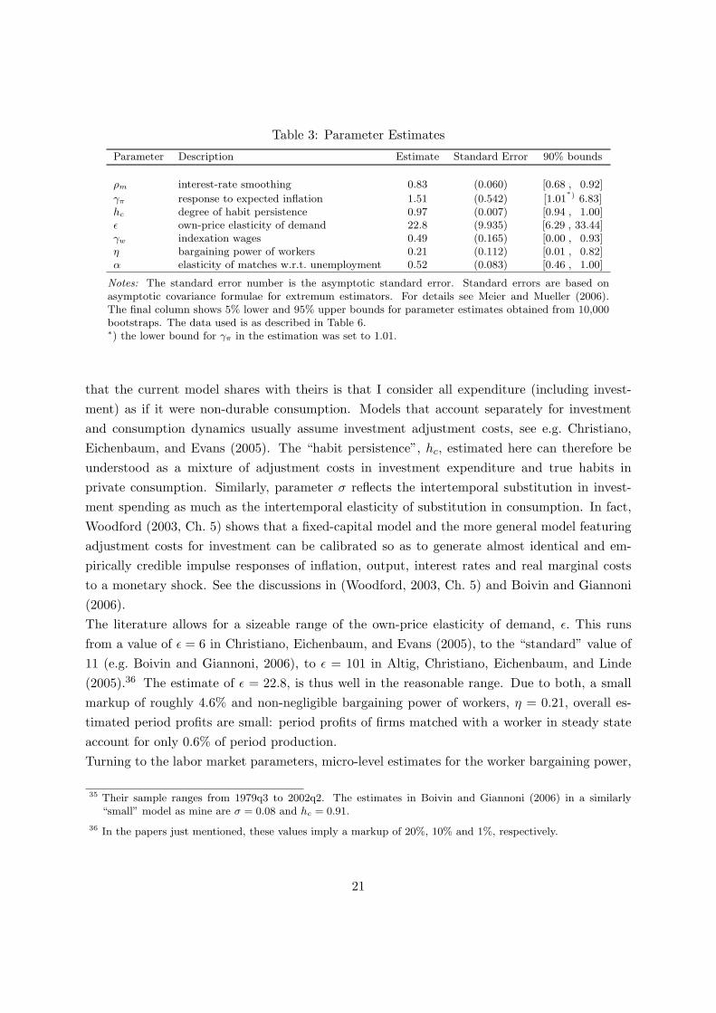
Table 3: Parameter Estimates

Parameter Description Estimate Standard Error 90% bounds

ρm interest-rate smoothing 0.83 (0.060) [0.68 , 0.92]

γπ response to expected inflation 1.51 (0.542) [1.01∗) 6.83]

hc degree of habit persistence 0.97 (0.007) [0.94 , 1.00]ǫ own-price elasticity of demand 22.8 (9.935) [6.29 , 33.44]γw indexation wages 0.49 (0.165) [0.00 , 0.93]η bargaining power of workers 0.21 (0.112) [0.01 , 0.82]α elasticity of matches w.r.t. unemployment 0.52 (0.083) [0.46 , 1.00]

Notes: The standard error number is the asymptotic standard error. Standard errors are based onasymptotic covariance formulae for extremum estimators. For details see Meier and Mueller (2006).The final column shows 5% lower and 95% upper bounds for parameter estimates obtained from 10,000bootstraps. The data used is as described in Table 6.∗) the lower bound for γπ in the estimation was set to 1.01.

that the current model shares with theirs is that I consider all expenditure (including invest-

ment) as if it were non-durable consumption. Models that account separately for investment

and consumption dynamics usually assume investment adjustment costs, see e.g. Christiano,

Eichenbaum, and Evans (2005). The “habit persistence”, hc, estimated here can therefore be

understood as a mixture of adjustment costs in investment expenditure and true habits in

private consumption. Similarly, parameter σ reflects the intertemporal substitution in invest-

ment spending as much as the intertemporal elasticity of substitution in consumption. In fact,

Woodford (2003, Ch. 5) shows that a fixed-capital model and the more general model featuring

adjustment costs for investment can be calibrated so as to generate almost identical and em-

pirically credible impulse responses of inflation, output, interest rates and real marginal costs

to a monetary shock. See the discussions in (Woodford, 2003, Ch. 5) and Boivin and Giannoni

(2006).

The literature allows for a sizeable range of the own-price elasticity of demand, ǫ. This runs

from a value of ǫ = 6 in Christiano, Eichenbaum, and Evans (2005), to the “standard” value of

11 (e.g. Boivin and Giannoni, 2006), to ǫ = 101 in Altig, Christiano, Eichenbaum, and Linde

(2005).36 The estimate of ǫ = 22.8, is thus well in the reasonable range. Due to both, a small

markup of roughly 4.6% and non-negligible bargaining power of workers, η = 0.21, overall es-

timated period profits are small: period profits of firms matched with a worker in steady state

account for only 0.6% of period production.

Turning to the labor market parameters, micro-level estimates for the worker bargaining power,

35 Their sample ranges from 1979q3 to 2002q2. The estimates in Boivin and Giannoni (2006) in a similarly“small” model as mine are σ = 0.08 and hc = 0.91.

36 In the papers just mentioned, these values imply a markup of 20%, 10% and 1%, respectively.

21

η, are hard to come by. On U.S. macro-data Trigari (2004) estimates η = 0.10, while Braun

(2005) gets η = 0.77. My estimate of η = 0.21 is in this range. Finally, for the elasticity of

matching with respect to unemployment, α, Petrongolo and Pissarides (2001) survey the liter-

ature to find that most estimates for the matching elasticity fall in the range from 0.5 to 0.7.37

My estimate of α = 0.52 is thus reasonable when judged by the micro-evidence.

Sampling Uncertainty of Parameters. The standard errors reported in Table 3 are based

on the asymptotic normality of the minimum-distance estimators. Complementary evidence on

the finite-sample distribution of the estimators can be obtained by bootstrapping. For each set

of impulse-responses obtained in the 10,000 bootstraps of the SVAR the model parameters are

re-estimated. Figure 2 shows histograms of the resulting sampling distribution of the parameters

and the final column of Table 3 reports 90% confidence intervals based on the sampling distri-

bution. Clearly, the advantage of this measure is that proper account is taken of the sampling

errors that result at each stage of the estimation. For about 9% of the estimates the lower bound

of 1.01 imposed for the monetary policy feedback to inflation, γπ, is binding. Most notable are

the implications for wage indexation and the bargaining power of workers. More than 40% of

the estimates for wage indexation, γw, end up at the lower bound of zero – wage indexation

does not seem to be a robust feature of my data set and model, in contrast to the case made

Christiano, Eichenbaum, and Evans (2005).38 Finally the bargaining power of workers, η has

a mode closer to zero than the point estimate in the benchmark SVAR suggests. Yet overall,

and abstracting from the asymmetry of some of the sampling distributions, the standard errors

reported in Table 3 give reasonable guidance to the uncertainty surrounding the point estimates

in the benchmark SVAR.

5 Conclusions

I have illustrated that with equilibrium unemployment and matching frictions strategic com-

plementarities in price setting naturally increase due to a temporarily firm-specific factor of

production: labor. The matching framework thus induces a significant amount of real price

rigidity as is needed to reconcile macro-estimates of Calvo-type Phillips curves with micro-

evidence. Besides, the same demand-factors that drive the real price rigidity translate into

significant amplification of real wage rigidity. The technical contribution of the paper was to

directly integrate the wage bargaining into a sector which has a margin for setting its price but

to retain ex-ante worker homogeneity.

37 In some of the studies reviewed therein, which use total hires as dependent variable (not only hires fromunemployment), the coefficient is lower ranging from 0.3 to 0.4.

38 It goes without mentioning that they have a very different model (and data span), of course.

22

In contrast to firm-specific capital models, say, the modified model implies cross-equation re-

strictions for a key parameter governing real rigidities (and thus identifies this parameter): the

elasticity of demand. For single equation Phillips-curve estimates the model implies (a) a time

discount-factor substantially smaller than unity (as is indeed commonly found in single equation

estimates of the New-Keynesian Phillips curve) due to the probability of separation of firm and

worker, the model implies (b) the presence of an employment gap as an additional (and usually

omitted) regressor and (c) small pass-through of aggregate developments to inflation, i.e. price-

durations in line with micro-evidence.

I find that the strategic complementarities in price-setting do not only induce inflation to be less

volatile than in the benchmark model. Most notably, the strategic complementarities also have a

bearing on the wage series. Even if wages are reset as frequently as prices (every second quarter

in my calibration), the resulting real wages series does not respond much to a sudden monetary

easing and to the associated increase in demand and labor market tightness. The smooth wage

series thus helps to replicate the fluctuations of vacancies found in U.S. data, which have been

the focus of much recent debate; see, for instance, Hall (2005) and Shimer (2004). A structural

VAR application to post Volcker disinflation U.S. data showed that the modified model can very

well replicate impulse responses to monetary policy shocks.

Throughout the analysis I have assumed that wages and prices are staggered a la Calvo and have

the same durations, i.e. prices are reset whenever wages are and vice versa. In this respect it

appears worth exploring to which extent the price and wage setting decisions can be uncoupled

in a way that still keeps heterogeneity tractable. In particular, real wage rates could be negoti-

ated in a state-contingent fashion. I leave this for future research – as well as an examination

of how these more flexible wages will affect vacancy fluctuations implied by the model.

23

Figure 2: Sampling Distribution of Parameters

ρm γπ hc

0.4 0.5 0.6 0.7 0.8 0.9 10

0.005

0.01

0.015

0.02

0.025

0.03

1 2 3 4 50

0.02

0.04

0.06

0.08

0.1

0.85 0.9 0.95 10

0.005

0.01

0.015

0.02

0.025

0.03

0.035

ǫ γw η

20 40 60 80 1000

0.01

0.02

0.03

0.04

0.05

0 0.2 0.4 0.6 0.8 10

0.1

0.2

0.3

0.4

0 0.2 0.4 0.6 0.8 10

0.01

0.02

0.03

0.04

0.05

0.06

α

0 0.2 0.4 0.6 0.8 10

0.02

0.04

0.06

0.08

0.1

Notes: The plots show histograms of the sampling distribution of the estimated parameters. On the setof impulse responses obtained in the 10,000 bootstraps underlying the grey areas of Figure 1 problem(38) is solved. The distribution of estimators bθ is plotted on the support of the respective parametersallowed for in the estimation. Exceptions are the plots for ρm,γπ, and hc. The estimation of γπ fixedthe upper bound at 60. 7.8% of the estimates were larger than the highest value of 5 plotted here. Theestimation of ρm allowed for a support between zero and one. However, no estimate was smaller thanthe lowest value reported in the plot. Similarly hc was estimated on [0,1) but no value was smaller thanthe lowest value reported. The vertical dashed red line in each graph marks the point estimate obtainedfrom the SVAR run on actual data (cp. Table 3). From top left to bottom right the graphs show thedistribution of estimates of the interest rate response to lagged interest rates and inflation, respectively,of habit persistence, the elasticity of demand, wage indexation, the bargaining power of workers and theelasticity of matching w.r.t. unemployment.

24

References

Abel, A. (1990): “Asset Prices under Habit Formation and Catching Up with the Joneses,”

American Economic Review, Papers and Proceedings, 80, 38–42.

Altig, D., L. Christiano, M. Eichenbaum, and J. Linde (2005): “Firm-Specific Capital,

Nominal Rigidities and the Business Cycle,” NBER Working Paper no. 11034.

Amato, J. D., and T. Laubach (2003): “Estimation and Control of an Optimization-Based

Model with Sticky Prices and Wages,” Journal of Economic Dynamics and Contral, 27(7),

1181–1215.

Ball, L., and D. Romer (1990): “Real Rigidities and the Non-neutrality of Money,” The

Review of Economic Studies, 57(2), 183–203.

Bils, M., and P. Klenow (2004): “Some Evidence on the Importance of Sticky Prices,”

Journal of Political Economy, 112(5), 947–985.

Boivin, J., and M. P. Giannoni (2006): “Has Monetary Policy Become More Effective?,”

The Review of Economics and Statistics, forthcoming.

Braun, H. (2005): “(Un)employment Dynamics: The Case of Monetary Policy Shocks,” mimeo;

Northwestern University.

Calvo, G. (1983): “Staggered Prices in a Utility Maximizing Framework,” Journal of Monetary

Economics, 12, 383–398.

Christiano, L. J. (2004): “Firm-Specific Capital and Aggregate Inflation Dynamics in Wood-

ford’s Model,” manuscript, www.faculty.econ.northwestern.edu / faculty / christiano / re-

search / firmspecific / svensson.pdf.

Christiano, L. J., M. Eichenbaum, and C. Evans (2005): “Nominal Rigidities and the

Dynamic Effects of a Shock to Monetary Policy,” Journal of Political Economy, 113(1), 1–45.

Christoffel, K., K. Kuester, and T. Linzert (2005): “The Impact of Labor Markets on

the Transmission Process of Monetary Policy,” IZA Discussion Paper No. 1902.

Clarida, R., J. Gali, and M. Gertler (1998): “Monetary Policy Rules in Practice. Some

International Evidence,” European Economic Review, 42(6), 1033–1067.

den Haan, W., G. Ramey, and J. Watson (2000): “Job Destruction and Propagation of

Shocks,” American Economic Review, 90, 482–498.

Dhyne, E., L. J. Alvarez, H. L. Bihan, G. Veronese, D. Dias, J. Hoffman, N. Jonker,

P. Lunnemann, F. Rumler, and J. Vilmunen (2005): “Price Setting in the Euro Area:

Some Stylized Facts From Individual Consumer Price Data,” ECB Working Paper No. 524.

25

Dotsey, M., R. King, and A. Wolman (1999): “State-Dependent Pricing and the General

Equilibrium Dynamics of Money and Output,” Quarterly Journal of Economics, 114(2), 655–

690.

Dridi, R., A. Guay, and E. Renault (2006): “Indirect Inference and Calibration of Dynamic

Stochastic General Equilibrium Models,” Journal of Econometrics, forthcoming.

Eichenbaum, M., and J. Fisher (2004): “Evaluating the Calvo Model of Sticky Prices,”

NBER Working Paper No. 10617.

Francis, N., and V. A. Ramey (2005): “Measures of Per Capita Hours and their Implications

for the Technology-Hours Debate,” NBER Working Paper No. 11694.

Fujita, S., and G. Ramey (2005): “The Dynamic Beveridge Curve,” Federal Reserve Bank of

Philadelphia, Working Paper No.05-22.

Gagnon, E., and H. Khan (2005): “New Phillips Curve under Alternative Production Tech-

nologies for Canada, the United States, and the Euro area,” European Economic Review,

49(6), 1571–1602.

Gali, J., and M. Gertler (1999): “Inflation Dynamics: A Structural Econometric Analysis,”

Journal of Monetary Economics, 44(2), 195–222.

Gali, J., M. Gertler, and D. Lopez-Salido (2001): “European Inflation Dynamics,” Eu-

ropean Economic Review, 45(7), 1237–1270.

Gali, J., and P. Rabanal (2004): “Technology Shocks and Aggregate Shocks: How Well does

the RBC Model Fit Postwar U.S. Data?,” NBER Working, No. 10636.

Gertler, M., and A. Trigari (2005): “Unemployment Fluctuations with Staggered Nash

Wage Bargaining,” mimeo; New York University.

Giannoni, M. P., and M. Woodford (2005): “Optimal Inflation Targeting Rules,” in The

Inflation-Targeting Debate, ed. by B. S. Bernanke, and M. Woodford, pp. 93–162. University

of Chicago Press, Chicago.

Gottschalk, P. (2004): “Downward Nominal Wage Flexibility: Real or Measurement Error?,”

IZA Discussion Paper No.1327.

Hagedorn, M., and I. Manovskii (2005): “The Cyclical Behavior of Equilib-

rium Unemployment and Vacancies Revisited,” mimeo; University of Pennsylvania.

www.econ.upenn.edu/∼manovski/papers/BCUV.pdf.

Hall, R. E. (1999): Labor-Market Frictions and Employment Fluctuations, pp. 1137–1170,

Handbook of Macroeconomics, vol. 1B. Elsevier, New York.

(2005): “Employment Fluctuations with Equilibrium Wage Stickiness,” American Eco-

nomic Review, 95(1), 50–65.

26

Kim, C.-J., and C. R. Nelson (1999): “Has the U.S. Economy Become More Stable? A

Bayesian Approach Based On a Markov-Switching Model of the Business Cycle,” The Review

of Economics and Statistics, 81(4), 608–616.

Kimball, M. (1995): “The Quantitative Analytics of the Basic Neomonetarist Model,” Journal

of Money, Credit and Banking, 27(4), 1241–1277.

Klenow, P., and O. Kryvtsov (2005): “State-Dependent or Time-Dependent Pricing: Does

it Matter for Recent U.S. Inflation,” NBER Working Paper No. 11043.

Krause, M., and T. Lubik (2006): “The (Ir)relevance of Real Wage Rigidity in the New

Keynesian Model with Search Frictions,” Journal of Monetary Economics, forthcoming.

McConnell, M., and G. Perez-Quiros (2000): “Output Fluctuations in the United States:

What has Changed Since the Early 1980’s?,” The American Economic Review, 90(5), 1464–

1476.

Meier, A., and G. Mueller (2006): “Fleshing out the Monetary Transmission Mechanism

- Output Composition and the Role of Financial Frictions,” Journal of Money, Credit and

Banking, forthcoming.

Mortensen, D., and E. Nagypal (2005): “More on Unemployment and Vacancy Fluctua-

tions,” NBER Working Paper No. 11692.

Mortensen, D., and C. Pissarides (1994): “Job Creation and Job Destruction in the Theory

of Unemployment,” Review of Economic Studies, 61(3), 397–415.

Petrongolo, B., and C. A. Pissarides (2001): “Looking into the Black Box: A Survey of

the Matching Function,” Journal of Economic Literature, 2001(2), 390–431.

Pissarides, C. (1985): “Short-Run Equilibrium Dynamics of Unemployment, Vacancies, and

Real Wages,” American Economic Review, 75(4), 676–690.

Ravn, M., S. Schmitt-Grohe, and M. Uribe (2006): “Deep Habits,” Review of Economic

Studies, forthcoming.

Rotemberg, J. J., and M. Woodford (1997): “An Optimization-Based Econometric Frame-

work for the Evaluation of Monetary Policy,” NBER Macroeconomics Annual, 12, 297–346.

Sbordone, A. (2002): “Prices and Unit Labor Costs: A New Test of Price Stickiness,” Journal

of Monetary Economics, 49(2), 265–292.

Shimer, R. (2004): “The Consequences of Rigid Wages in Search Models,” Journal of the

European Economic Association, 2(2).

Smets, F., and R. Wouters (2003): “An Estimated Stochastic Dynamic General Equilibrium

Model of the Euro Area,” Journal of the European Economic Association, 1(5), 1123–75.

27

Stock, J., and M. Watson (2002): “Has the Business Cycle Changed and Why?,” NBER

Working Papers 9127, National Bureau of Economic Research.

Sveen, T., and L. Weinke (2004): “Pitfalls in the Modeling of Forward-Looking Price Setting

and Investment Decisions,” Universitat Pompeu Fabra Working Paper No. 773.

Taylor, J. B. (1999): Staggered Price and Wage Setting in Macroeconomics, pp. 1009–1050,

Handbook of Macroeconomics, vol. 1B. Elsevier, New York.

Trigari, A. (2004): “Equilibrium Unemployment, Job Flows and Inflation Dynamics,” ECB

Working Paper No. 304.

Woodford, M. (2003): Interest and Prices: Foundations of a Theory of Monetary Policy.

Princeton University Press, Princeton.

(2005): “Firm-Specific Capital and the New-Keynesian Phillips Curve,” International

Journal of Central Banking, 1(2), 1–46.

Yashiv, E. (2005): “Evaluation the Performance of the Search and Matching Model,” CEPR

Discussion Paper no. 677.

28

A Steady State and Calibration

The following sixteen equations (40) to (55) jointly characterize the steady state of the model.

A.1 Household conditions

Real rate: By Euler equation (4)

R =1

β. (40)

Marginal utility of consumption:

λ = (1 − hc)−σy−σ. (41)

Marginal rate of substitution:

mrs = κhhφ

λ. (42)

Surplus of the worker: by equation (19)

∆ =wh− mrs

1+φh− b

1 − β(1 − ρ)(1 − s). (43)

A.2 Firm conditions

Value of the firm: by equation (13)

J =ya − wh

1 − β(1 − ρ). (44)

Vacancy posting: by equation (10)

J =κ

βq(1 − ρ). (45)

Wage FOC: by equation (22), using the steady state expressions for the partial derivatives

involved,

ηJ = (1 − η)∆. (46)

Price FOC: by equation (21), using the steady state expressions for the partial derivatives

involved,

mrs =ǫ− 1

ǫz. (47)

A.3 Matching Market

Number of employees: by equation (15)

ρn = (1 − ρ)m. (48)

29

Number of unemployed: by equation (16)

u = 1 − n. (49)

Number of matches: by equation (14)

m = σm uαv1−α. (50)

Probability of finding a job:

s =m

u. (51)

Probability of finding a worker:

q =m

v. (52)

A.4 Goods market clearing

Average production:

ya = zh. (53)

Final good supply: by equation (27)

y = nzh. (54)

Final good demand: by equation (26)

c = y. (55)

A.5 Calibration

The model has four free parameters: the disutility of work scaling factor, κh, vacancy posting

costs, κ, the efficiency of matching, σm, and the unemployment benefit (including the value of

home production), b. I normalize z to unity. I fix a steady state unemployment rate as described

in Table 2 and choose a value of 1/3 for hours worked as well as the probability of finding a

worker, q, and the replacement rate, bwh, as both described in Table 2. Using the other calibrated

and estimated parameters in Tables 2 and 3 this implicitly defines the free parameters and the

steady state values of all endogenous variables.

B Source of Data

All data are taken from the Federal Reserve Board of St. Louis database FRED except for the

adjusted labor force series by Francis and Ramey (2005), which was supplied by these authors

and is given mnemonic LABFFR below, and wage and salary disbursements (private industry),

which is taken from the Bureau of Economic Analyis NIPA data and carries mnemonic A132RC1

below.

30

Table 4: Data Description and Sources Benchmark Model

Mnemonic Data description

Vacancies HELPWANT Index of Help-Wanted Advertisingbase year 1987=100, seasonally adjustedquarterly average of monthly figures (own).

Interest rate FEDFUNDS Effective Federal Funds Ratemonthly average, % p.a.quarterly average of monthly figures (own).

Nominal wage rate AHETPI Average Hourly Earnings: Total Private Industriesmonthly, seasonally adjusted, dollars per hourquarterly average of monthly figures (own).

Labor Force CLF16OV Civilian Labor Force, 16 years and overmonthly, seasonally adjusted, thousandsquarterly average of monthly figures (own).

Total hours worked HOABS Business Sector: Hours of all Personsquarterly, seasonally adjustedindex 1992=100.

Unemployment rate UNRATE Civilian Unemployment Ratemonthly, seasonally adjusted,quarterly average of monthly figures (own).

Real output GDPC96 Real Gross Domestic Productquarterly, seasonally adjusted annual ratesbillions of chained 2000 dollars.

GDP deflator GDPDEF Gross Domestic Product: Implicit Price Deflatorquarterly, seasonally adjustedindex 2000=100.

Consumer price index PCECTPI Personal Consumption Expenditures: Chain-Type Price Indexquarterly, seasonally adjustedindex 2000=100.

31

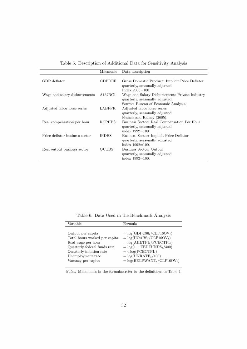
Table 5: Description of Additional Data for Sensitivity Analysis

Mnemonic Data description

GDP deflator GDPDEF Gross Domestic Product: Implicit Price Deflatorquarterly, seasonally adjustedIndex 2000=100.

Wage and salary disbursements A132RC1 Wage and Salary Disbursements Private Industryquarterly, seasonally adjusted,Source: Bureau of Economic Analysis.

Adjusted labor force series LABFFR Adjusted labor force seriesquarterly, seasonally adjustedFrancis and Ramey (2005).

Real compensation per hour RCPHBS Business Sector: Real Compensation Per Hourquarterly, seasonally adjustedindex 1992=100.

Price deflator business sector IPDBS Business Sector: Implicit Price Deflatorquarterly, seasonally adjustedindex 1992=100.

Real output business sector OUTBS Business Sector: Outputquarterly, seasonally adjustedindex 1992=100.

Table 6: Data Used in the Benchmark Analysis

Variable Formula

Output per capita = log(GDPC96t/CLF16OVt)Total hours worked per capita = log(HOABSt/CLF16OVt)Real wage per hour = log(AHETPIt/PCECTPIt)Quarterly federal funds rate = log(1 + FEDFUNDSt/400)Quarterly inflation rate = d log(PCECTPIt)Unemployment rate = log(UNRATEt/100)Vacancy per capita = log(HELPWANTt/CLF16OVt)

Notes: Mnemonics in the formulae refer to the definitions in Table 4.

32

Table 7: Data Used in the Sensitivity Analysis

Variable Formula

Case 2

Output per capita = log(GDPC96t/CLF16OVt)Total hours worked per capita = log(HOABSt/CLF16OVt)Real wage per hour = log(AHETPI.t/GDPDEFt)Quarterly federal funds rate = log(1 + FEDFUNDSt/400)Quarterly inflation rate = d log(PCECTPIt)Unemployment rate = log(UNRATEt/100)Vacancy per capita = log(HELPWANTt/CLF16OVt)

Case 3

Output per capita = log(GDPC96t/CLF16OVt)Total hours worked per capita = log(HOABSt/CLF16OVt)Real wage per hour = log(A132RC1t/PCECTPIt/HOABSt)Quarterly federal funds rate = log(1 + FEDFUNDSt/400)Quarterly inflation rate = d log(PCECTPIt)Unemployment rate = log(UNRATEt/100)Vacancy per capita = log(HELPWANTt/CLF16OVt)

Case 4

Output per capita = log(OUTBSt/LABFFRt)Total hours worked per capita = log(HOABSt/LABFFRt)Real wage per hour = log(RCPHBSt ∗ IPDBSt/PCECTPIt)Quarterly federal funds rate = log(1 + FEDFUNDSt/400)Quarterly inflation rate = d log(PCECTPIt)Unemployment rate = log(UNRATEt/100)Vacancy per capita = log(HELPWANTt/LABFFRt)

Notes: Mnemonics in the formulae refer to the definitions in Tables 4 and 5.

33

C Sensitivity

C.1 Case 2

Table 8: Parameter Estimates Sensitivity Case 2

Parameter Description Estimate Standard Error

ρm interest-rate smoothing 0.82 (0.059)γπ response to expected inflation 1.35 (0.414)hc degree of habit persistence 0.97 (0.008)ǫ own-price elasticity of demand 22.8 (9.197)γw indexation wages 0.53 (0.146)η bargaining power of workers 0.23 (0.117)α elasticity of matches w.r.t. unemployment 0.50 (0.082)

Notes: Parameter Estimates. The weighting matrix is obtained by 1,000 bootstraps fromthe estimated SVAR. The numbers reported for standard errors are the asymptotic stan-dard errors. Standard errors are based on asymptotic covariance formulae for extremumestimators. For details see Meier and Mueller (2006). The data used is as described inTable 7.

34

Figure 3: Impulse Responses - Sensitivity Case 2

yt πt vt ut

0 5 10 15−2

−1

0

1

2

3

4

0 5 10 15

−0.4

−0.2

0

0.2

0.4

0.6

0.8

0 5 10 15−40

−20

0

20

40

0 5 10 15−40

−30

−20

−10

0

10

20

ht wt Rt wt + ht + nt

0 5 10 15

−4

−2

0

2

4

0 5 10 15

−1.5

−1

−0.5

0

0.5

1

1.5

0 5 10 15

−1

−0.5

0

0.5

1

0 5 10 15

−5

0

5

Notes: The plots show impulse responses to a unit monetary policy shock. All variables are in percentagedeviation from their respective steady state values. The solid black line corresponds to the empirical impulseresponse estimated in a VAR(4) from 1984q1 to 2005q3 (including lags up to 1983q1). The red dotted linemarks the impulse response from the estimated DSGE model. Shaded areas pertain to 90% bootstrappedsymmetric confidence intervals from 1,000 draws (computed as ±1.645 the bootstrapped standard deviation).From top left to bottom right the graphs show the responses of: output gap, inflation rate, vacancies,unemployment rate, total hours worked, real wage rate and gross nominal interest rate. The bottom rightplot reports the implied response of total wages which was not used in the estimation exercise but is reportedfor completeness. The data used is as described in Table 7.

35

C.2 Case 3

Table 9: Parameter Estimates Sensitivity Case 3

Parameter Description Estimate Standard Error

ρm interest-rate smoothing 0.81 (0.060)γπ response to expected inflation 1.29 (0.354)hc degree of habit persistence 0.97 (0.009)ǫ own-price elasticity of demand 20.7 (8.422)γw indexation wages 0.59 (0.152)η bargaining power of workers 0.34 (0.177)α elasticity of matches w.r.t. unemployment 0.53 (0.074)

Notes: Parameter Estimates. The weighting matrix is obtained by 1,000 bootstraps fromthe estimated SVAR. The numbers reported for standard errors are the asymptotic stan-dard errors. Standard errors are based on asymptotic covariance formulae for extremumestimators. For details see Meier and Mueller (2006). The data used is as described inTable 7.

36

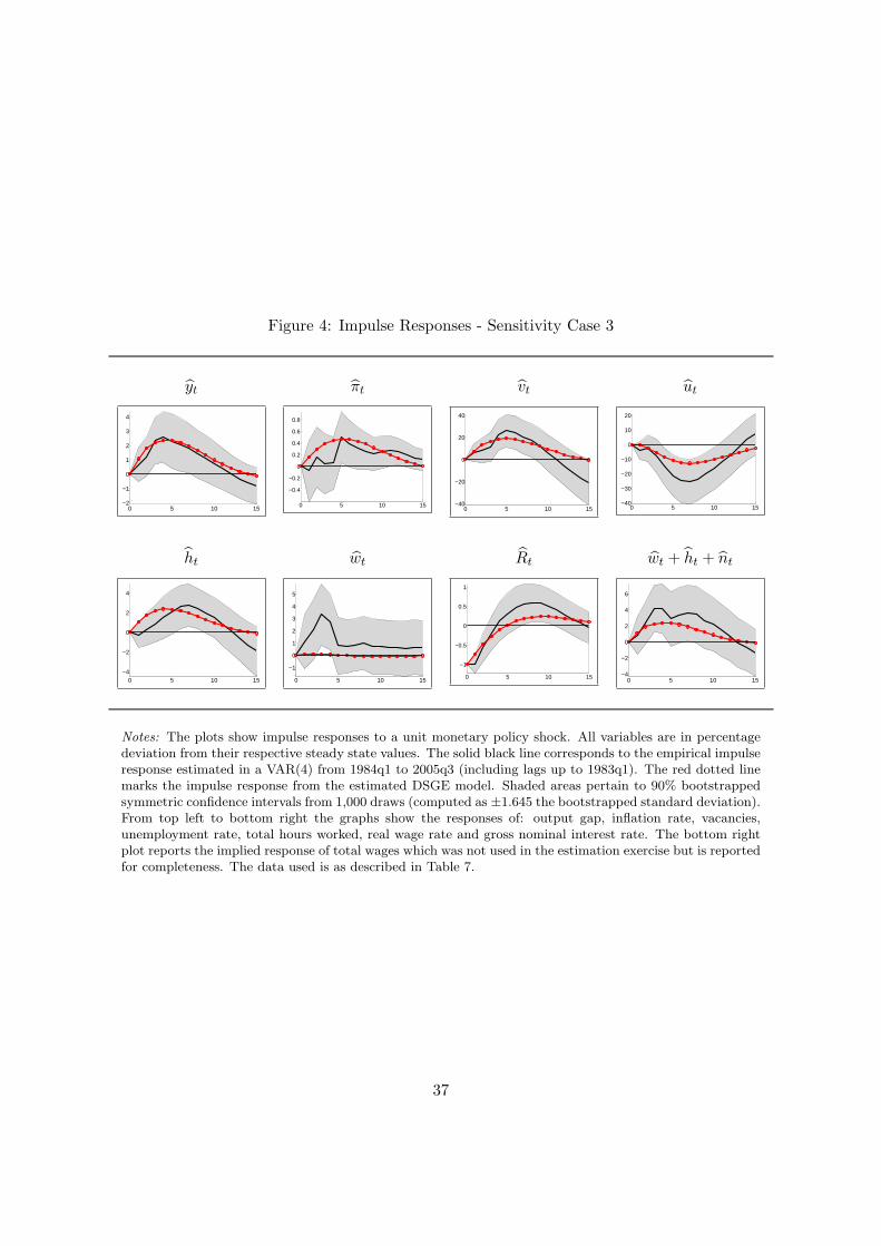
Figure 4: Impulse Responses - Sensitivity Case 3

yt πt vt ut

0 5 10 15−2

−1

0

1

2

3

4

0 5 10 15

−0.4

−0.2

0

0.2

0.4

0.6

0.8

0 5 10 15−40

−20

0

20

40

0 5 10 15−40

−30

−20

−10

0

10

20

ht wt Rt wt + ht + nt

0 5 10 15−4

−2

0

2

4

0 5 10 15

−1

0

1

2

3

4

5

0 5 10 15

−1

−0.5

0

0.5

1

0 5 10 15−4

−2

0

2

4

6

Notes: The plots show impulse responses to a unit monetary policy shock. All variables are in percentagedeviation from their respective steady state values. The solid black line corresponds to the empirical impulseresponse estimated in a VAR(4) from 1984q1 to 2005q3 (including lags up to 1983q1). The red dotted linemarks the impulse response from the estimated DSGE model. Shaded areas pertain to 90% bootstrappedsymmetric confidence intervals from 1,000 draws (computed as ±1.645 the bootstrapped standard deviation).From top left to bottom right the graphs show the responses of: output gap, inflation rate, vacancies,unemployment rate, total hours worked, real wage rate and gross nominal interest rate. The bottom rightplot reports the implied response of total wages which was not used in the estimation exercise but is reportedfor completeness. The data used is as described in Table 7.

37

C.3 Case 4

Table 10: Parameter Estimates Sensitivity Case 4

Parameter Description Estimate Standard Error

ρm interest-rate smoothing 0.82 (0.071)γπ response to expected inflation 1.83 (0.884)hc degree of habit persistence 0.96 (0.012)ǫ own-price elasticity of demand 22.2 (10.454)γw indexation wages 0.45 (0.214)η bargaining power of workers 0.34 (0.182)α elasticity of matches w.r.t. unemployment 0.48 (0.069)

Notes: Parameter Estimates. The weighting matrix is obtained by 1,000 bootstraps fromthe estimated SVAR. The numbers reported for standard errors are the asymptotic stan-dard errors. Standard errors are based on asymptotic covariance formulae for extremumestimators. For details see Meier and Mueller (2006). The data used is as described inTable 7.

38

Figure 5: Impulse Responses - Sensitivity Case 4

yt πt vt ut

0 5 10 15

−2

−1

0

1

2

3

4

5

0 5 10 15

−0.4

−0.2

0

0.2

0.4

0.6

0.8

0 5 10 15

−20

−10

0

10

20

30

0 5 10 15−30

−20

−10

0

10

ht wt Rt wt + ht + nt

0 5 10 15

−2

−1

0

1

2

3

4

5

0 5 10 15

−3

−2

−1

0

1

2

3

0 5 10 15

−1

−0.5

0

0.5

0 5 10 15

−2

0

2

4

Notes: The plots show impulse responses to a unit monetary policy shock. All variables are in percentagedeviation from their respective steady state values. The solid black line corresponds to the empirical impulseresponse estimated in a VAR(4) from 1984q1 to 2004q3 (including lags up to 1983q1). The red dotted linemarks the impulse response from the estimated DSGE model. Shaded areas pertain to 90% bootstrappedsymmetric confidence intervals from 1,000 draws (computed as ±1.645 the bootstrapped standard deviation).From top left to bottom right the graphs show the responses of: output gap, inflation rate, vacancies,unemployment rate, total hours worked, real wage rate and gross nominal interest rate. The bottom rightplot reports the implied response of total wages which was not used in the estimation exercise but is reportedfor completeness. The data used is as described in Table 7.

39