REAL OPTION ANALYSIS OF PRIMARY RAIL CONTRACTS IN …
132
REAL OPTION ANALYSIS OF PRIMARY RAIL CONTRACTS IN GRAIN SHIPPING A Thesis Submitted to the Graduate Faculty of the North Dakota State University of Agriculture and Applied Science By Daniel Jacob Landman In Partial Fulfillment of the Requirements for the Degree of MASTER OF SCIENCE Major Department: Agribusiness & Applied Economics April 2017 Fargo, North Dakota
Transcript of REAL OPTION ANALYSIS OF PRIMARY RAIL CONTRACTS IN …

REAL OPTION ANALYSIS OF PRIMARY RAIL CONTRACTS IN GRAIN SHIPPING
A Thesis Submitted to the Graduate Faculty
of the North Dakota State University
of Agriculture and Applied Science
By
Daniel Jacob Landman
In Partial Fulfillment of the Requirements for the Degree of
MASTER OF SCIENCE
Major Department: Agribusiness & Applied Economics
April 2017
Fargo, North Dakota

North Dakota State University Graduate School
Title
Real Option Analysis of Primary Rail Contracts in Grain Shipping
By
Daniel Jacob Landman
The Supervisory Committee certifies that this disquisition complies with North Dakota
State University’s regulations and meets the accepted standards for the degree of
MASTER OF SCIENCE
SUPERVISORY COMMITTEE:
Dr. William Wilson
Chair
Dr. Frayne Olson
Dr. Fariz Huseynov
Approved: April 13, 2017 Dr. William Nganje Date Department Chair

iii
ABSTRACT
Grain shipping for a country elevator involves many sources of risk and uncertainty. In
response to these dynamic challenges faced by shippers, railroad carriers offer various types of
forward contracting instruments and shuttle programs. Certain contracting instruments provide
managerial flexibility by allowing shippers to sell excess railcars into a secondary market. The
purpose of this study is to value this transferability as a European put option. A framework is
developed around a material requirement planning schedule and real option analysis to represent
the strategic decisions facing a primary shuttle contract owner. Monte Carlo simulation is
incorporated with a stochastic binomial option pricing model to value the transfer option. A
sensitivity analysis is then conducted to determine the impact of key input variables. This study
provides insights about railcar ordering strategy, and the implications of transferable rail
contracts for shippers and carriers.

iv
ACKNOWLEDGEMENTS
I would like to thank my advisor, Dr. Bill Wilson, for his support in this research, as well
as guidance in both scholastic and professional endeavors. Working with him has been a
rewarding experience, as he recognizes that professional success requires more than classroom
experience. I am grateful for my committee members, Dr. Frayne Olson and Dr. Fariz Huseynov,
who have taken time out of their busy schedules to provide constructive criticism in this project.
I’m also thankful for Bruce Dahl, who provided assistance with data collection.
Thank you to my fellow classmates and colleagues within the Agribusiness & Applied
Economics department. Many of these friendships have extended beyond the classroom,
especially with Dr. William Nganje, who proved to be a worthy opponent in the racquetball
court. I also extend my gratitude to the industry sources who answered my numerous questions
without hesitation. These have included Kirk Gerhardt, David Pope, Levi Hall, Dan Mostad,
John Crabb, and many others.
A special thanks to all of my friends and family outside of school as well. Whether it was
adventures in foreign countries, or memorable nights here in Fargo, college would not have been
nearly as enjoyable without them. The unwavering support of my parents, Bob and Karen, has
allowed me to pursue ventures near and afar, but also have the comfort that there will always be
a warm bed for me at home on the farm.

v
TABLE OF CONTENTS
ABSTRACT ................................................................................................................................... iii
ACKNOWLEDGEMENTS ........................................................................................................... iv
LIST OF TABLES ......................................................................................................................... ix
LIST OF FIGURES ........................................................................................................................ x
CHAPTER 1. INTRODUCTION ................................................................................................... 1
1.1.Overview ........................................................................................................................... 1
1.2.Problem Statement ............................................................................................................ 1
1.2.1.Inventory Level Risk ......................................................................................... 2
1.2.2.Railroad Price Risk ............................................................................................ 4
1.2.3.Railroad Performance Risk ................................................................................ 7
1.2.4.2013/2014 Situation ........................................................................................... 9
1.3.Objectives ....................................................................................................................... 11
1.4.Procedures ....................................................................................................................... 11
1.5.Organization .................................................................................................................... 13
CHAPTER 2. RAIL SHIPPING IN GRAIN: BACKGROUND AND PRIOR STUDIES .......... 14
2.1.Introduction ..................................................................................................................... 14
2.2.Evolution of Rail Pricing and Service Mechanisms ....................................................... 16
2.3.Current Pricing and Service Mechanisms ....................................................................... 19
2.3.1.Primary vs. Secondary Markets in General ..................................................... 19
2.3.2.Mechanisms Relevant to This Study ............................................................... 20
2.3.3.BNSF Shuttle Program .................................................................................... 25
2.3.4.Secondary Market ............................................................................................ 28

vi
2.4.Central Freight Desk System .......................................................................................... 29
2.5.Previous Studies on Rail Pricing Mechanisms ............................................................... 32
2.5.1.Impact of Rail Rates on Grain Shippers and Producers ................................... 32
2.5.2.Railcar Allocation Mechanism Design & Pricing ........................................... 34
2.5.3.Rail Pricing and Logistical Supply Chain Management .................................. 36
2.6.Summary ......................................................................................................................... 37
CHAPTER 3. REAL OPTION ANALYSIS: BACKGROUND AND PRIOR STUDIES .......... 39
3.1.Introduction ..................................................................................................................... 39
3.2.Real Option Analysis Overview ..................................................................................... 39
3.2.1.ROA vs. NPV .................................................................................................. 40
3.2.2.Real Options vs. Financial Options ................................................................. 41
3.3.Types and Examples of Real Options ............................................................................. 43
3.4.General Methods of Calculating Real Option Values .................................................... 45
3.5.Methods Relevant to this Study ...................................................................................... 47
3.5.1.Railcars as a Transfer Option ........................................................................... 47
3.5.2.Binomial Option Pricing Model ...................................................................... 50
3.6.Real Option Analysis in Prior Studies ............................................................................ 52
3.6.1.Early Real Option Studies ................................................................................ 52
3.6.2.Real Option Analysis in Agriculture ............................................................... 53
3.6.3.Real Option Analysis in Shipping ................................................................... 55
3.7.Conclusion ...................................................................................................................... 56
CHAPTER 4. EMPIRICAL MODEL FOR THE TRANSFER OPTION .................................... 57
4.1.Introduction ..................................................................................................................... 57

vii
4.2.Basic Model Overview ................................................................................................... 57
4.3.Detailed Elements of Model ........................................................................................... 60
4.3.1.MRP Module Details ....................................................................................... 60
4.3.2.Stochastic Binomial Option Pricing Module Details ....................................... 65
4.4.Model Setup .................................................................................................................... 70
4.5.Data Sources and Distributions ....................................................................................... 72
4.5.1.Description of Data and Sources ..................................................................... 72
4.5.2.Stochastic Distributions ................................................................................... 73
4.6.Summary ......................................................................................................................... 77
CHAPTER 5. RESULTS .............................................................................................................. 78
5.1.Introduction ..................................................................................................................... 78
5.2.Base Case Results ........................................................................................................... 79
5.3.Sensitivity Analysis on Stochastic Variables .................................................................. 85
5.3.1.Sensitivity – Secondary Market Prices ............................................................ 86
5.3.2.Sensitivity – Shipping Demand Volatility ....................................................... 87
5.3.3.Sensitivity - Rail Velocity ................................................................................ 89
5.3.4.Sensitivity – Futures Price Spreads ................................................................. 92
5.3.5.Sensitivity – 2013/2014 Scenario .................................................................... 94
5.4.Strategic Sensitivity – Railcar Ordering Strategy ........................................................... 95
5.5.Summary ......................................................................................................................... 97
CHAPTER 6. CONCLUSION ..................................................................................................... 99
6.1.Introduction ..................................................................................................................... 99
6.2.Problem Statement ........................................................................................................ 100

viii
6.3.Current Railroad Pricing/Contracting Mechanisms ...................................................... 102
6.4.Real Option Pricing Methodology ................................................................................ 104
6.5.Empirical Model ........................................................................................................... 105
6.6.Results ........................................................................................................................... 107
6.6.1.Conclusions from Base Case ......................................................................... 108
6.6.2.Conclusions from Sensitivity Analysis .......................................................... 109
6.7.Implications of Results ................................................................................................. 110
6.7.1.Implications for Shippers ............................................................................... 110
6.7.2.Implications for Carriers ................................................................................ 112
6.8.Summary ....................................................................................................................... 112
6.8.1.Contribution to Literature .............................................................................. 113
6.8.2.Limitations ..................................................................................................... 113
6.8.3.Further Research ............................................................................................ 115
REFERENCES ........................................................................................................................... 117

ix
LIST OF TABLES
Table Page
2.1. BNSF Car Ordering Programs (bnsf.com) ............................................................................. 22
3.1. Financial Options vs. Real Options (Trigeorgis 1996) .......................................................... 43
4.1. Five Components of Transfer Option .................................................................................... 58
4.2. Shipping Demand Schedule Example .................................................................................... 63
4.3. January Option Inputs ............................................................................................................ 66
4.4. Base Case Inputs .................................................................................................................... 71
4.5. Futures Prices ......................................................................................................................... 71
4.6. Inputs for Sensitivity Analysis ............................................................................................... 72
4.7. Outputs to Evaluate ................................................................................................................ 72
4.8. Stochastic Variable Information (@Risk).............................................................................. 74
4.9. Correlation Matrix (@Risk) ................................................................................................... 74
5.1. Base Case Results .................................................................................................................. 80
5.2. Sensitivity - Secondary Rail Market Prices ........................................................................... 87
5.3. Sensitivity - Shipping Demand Volatility .............................................................................. 88
5.4. Sensitivity - Rail Velocity ...................................................................................................... 90
5.5. Sensitivity - Futures Price Spreads ........................................................................................ 93
5.6. Sensitivity - 2013/2014 Scenario ........................................................................................... 95
5.7. Sensitivity - Railcar Ordering Strategy .................................................................................. 97
6.1. Summary of Results ............................................................................................................. 110

x
LIST OF FIGURES
Figure Page
1.1. Secondary Railcar Prices (TradeWest Brokerage Co., compiled by Bruce Dahl) ................... 6
1.2. Historical Tariff Rates from Casselton to Tacoma (USDA-AMS GTR Report) ..................... 6
2.1. Typical Flow of Grain Through the Supply Chain ................................................................ 15
2.2. BNSF Historical Performance (bnsf.com) ............................................................................. 26
2.3. Bid/Offer Sheet for Secondary Market (Courtesy of TradeWest Brokerage Co.) ................. 29
2.4. Freight Desk System Flowchart ............................................................................................. 31
3.1. Relationship of Put Options and Railcar Transferability ....................................................... 49
3.2. Generic One-Branch Lattice Tree .......................................................................................... 51
3.3. Generic Extended Lattice Tree .............................................................................................. 51
4.1. Module Flow .......................................................................................................................... 60
4.2. Railcar Choice Alternatives ................................................................................................... 68
4.3. January Transfer Option ........................................................................................................ 70
4.4. PNW Basis Sample Path (@Risk) ......................................................................................... 75
4.5. Farmer Sales Percent Sample Path (@Risk) .......................................................................... 75
4.6. Secondary Rail Market Sample Path (@Risk) ....................................................................... 76
4.7. Velocity Sample Path (@Risk) .............................................................................................. 76
5.1. Base Case Distribution of Results (@Risk) ........................................................................... 81
5.2. Option Values and Shipping Demand .................................................................................... 82
5.3. Option Values and Railcar Velocity ...................................................................................... 83
5.4. Impact of Key Inputs on Option Value (@Risk) ................................................................... 84
5.5. Correlations of Key Inputs with Option Value (@Risk) ....................................................... 84

xi
5.6. Maximum Payoff Percentage ................................................................................................. 85
5.7. Shipping Demand Volatility & Option Values (@Risk) ....................................................... 89
5.8. Velocity Distribution - All Months (@Risk) ......................................................................... 90
5.9. Option Values and Velocity ................................................................................................... 91
5.10. Sensitivity - Futures Price Spreads and Shipping Demand (@Risk) ................................... 93
6.1. Base Case Distribution of Option Values (@Risk) ............................................................. 109

1
1 CHAPTER 1. INTRODUCTION
1.1. Overview
Increased volatility in the market for railcar demand has required grain shippers to pay
more attention to their car ordering strategies. Their approach to ordering railcars can be the
difference between efficient commodity movement through the supply chain, or piles of grain
sitting on the ground outside with nowhere to go. This can be due to the shipper not having
enough storage, not having enough cars ordered to meet their shipping demand, or the cars they
have ordered being late due to bottlenecks. In response to these numerous risks, railroad
companies offer various contracting instruments to grain shippers. These contracts differ from
carrier to carrier, and change over time. Among these contract agreements are different terms and
conditions, some of which provide shippers with managerial flexibility. The flexibility in this
study refers to the options a shipper is provided with when they have excess railcars on hand.
While traditional methods, such as net present value (NPV) analysis, provide tools to value the
quantitative aspects of these contracts, valuing the qualitative components provide more of a
challenge. One emerging capital budgeting method to value the flexibility embedded within
investment decision making is real option analysis. This chapter highlights the logistical risks
inherent in grain shipping, objectives of this study, procedures, and organization of the paper.
1.2. Problem Statement
Just as buyers and sellers of a commodity are exposed to price risk of the commodity
itself, they are also exposed to logistical risk in each step of the supply chain (Wilson & Dahl
2011). The logistics process involves multiple steps, and each one is crucial to the overall goal or
objective of the business. In many logistics systems, if any step in the process underperforms, the
whole system itself is at risk of failing (Choi, Chiu, & Chan 2016). This is especially important

2
in grain markets. as there are usually many steps involved between the initial producer, and the
final consumer.
Take for example a soybean crush plant in China who has bought soybeans for delivery
in a specified month. If these soybeans are coming from an exporter in the U.S., they would have
been loaded on an ocean vessel at a port. Prior to this, the soybeans may have been sourced from
an inland country elevator. If the railroad carrier that is hauling the grain from the elevator to the
port experiences delays, the grain is late to the port. This in turn causes issues for the ocean
vessel, since it must either wait for the grain, or move on without it. Either way, this forces the
soybean crusher in China to either wait for the grain, whilst possibly delaying production, or
source the soybeans from elsewhere, exposing them to the price risk of other markets.
In an industry as dynamic as grain merchandising, managers face many different
decisions, and each of these decisions involves some level of risk. When it comes to ordering
railcars, there are various sources of uncertainty that can affect returns to a shipper. Among
many, three of the major sources risk stem from the fact that: 1) farmer deliveries (i.e. inventory
levels) are unknown for certain, 2) prices of railcar service changes daily, and 3) railroad
performance can fluctuate. The issue of rail performance has recently been at the forefront of
grain shipping in the 2013/2014 marketing year when various factors caused large backlogs of
grain, which is discussed later in this chapter.
1.2.1. Inventory Level Risk
The first issue, random inventory levels, stems from the fact that farmers do not always
deliver grain according to a set schedule. Although elevators offer a variety of contracts to their
producers that ensure grain delivery during a given timeframe, a large portion of farmer sales are
the result of “cash” or “spot” deliveries. These sales occur when farmers decide that the current

3
price posted by the elevator is sufficient for their needs, and sell grain on the “spot” by hauling it
in and transferring ownership. Given the fact that farmers naturally sell more grain when prices
are high yields the notion that elevators can control supply levels to some degree by raising or
lowering their bids. Although this is true to some extent, elevators cannot directly dictate 100%
of supply levels since the decision to sell in a spot sale is ultimately up to the farmer. Also,
adding to the uncertainty is the fact that elevators do not exactly set the full price of grain.
Rather, they set their “basis” value, which is premium or discount in relation to the futures
market price of a commodity. The futures price, which is traded on a central exchange, typically
serves as a regional or global benchmark price for a given month (Bernard, Khalaf, Kichian, &
McMahon 2015). When elevators are in need of grain, they may increase their basis in order to
attract farmer sales. However, a simultaneous decrease in futures prices may cause the posted
cash price for the day to remain unchanged. This gives elevators even less control as to how
much grain inventory they are able to purchase from farmers. Due to the fact that many railroad
carriers offer yearlong contracts, this means that elevator mangers must make car ordering
decisions for months or years in advance to ship inventory that they are unsure that they will
have. Alternatively, if a shipper does not order enough cars, they may not be able to move grain
in a timely manner and could be forced to halt farmer sales.
When farmers deliver grain, the elevator, who is exposed to cash price risk, can offset
most of this risk by hedging in futures markets (Myers & Hanson 1996). The elevator is then
exposed to basis risk. One of the only ways for an elevator to ensure supply levels and price is to
issue forward contracts to producers, which specify the number of bushels, price, and time of
delivery. These contracts are attractive to both parties since producers can mitigate price risk and
they assure a supply of grain for the elevator (Mark, Brorsen, Anderson, & Small 2008).

4
Elevators also buy grain on “Delayed Price” contracts, which gives the elevator control of the
grain, but allows the farmer to set the price later. Since a typical country elevator cannot forward
contract 100% of farmer deliveries, they are almost always exposed to some degree of inventory
risk.
1.2.2. Railroad Price Risk
The second major source of logistic uncertainty facing elevators is the fact that prices for
rail service fluctuate monthly or daily (depending on the carrier and pricing mechanism). Rail
rates are comprised of three main elements: tariff, primary auction price, and the secondary
market rate. A shipper who forward contracts cars directly with the rail carrier pays the tariff and
the primary auction price. Shippers who do not forward contract with the railroad, and instead
utilize cars on an as-needed basis, pay the tariff and secondary market rate. Volatilities of tariff
rates and primary auction rates are minimal, but secondary market rates fluctuate significantly.
The primary market allows the shipper to forward contract cars for a year at a stable
price, but an elevator who has not contracted or locked in a forward price for rail service is
exposed to potential rate changes every time they ship grain. In the BNSF pricing model, as well
as most other major railroad carriers, shippers each pay a tariff rate that is posted for every origin
and destination combination. This tariff rate is the base amount that the shipper pays to BNSF for
rail service, which is meant to cover the cost of rail service, margin, and possibly a fuel service
charge (bnsf.com). The fuel service charge is meant to be a variable part of the tariff that
fluctuates with the price of fuel. Some carriers explicitly list this charge, and others build it into
their tariff rate. This tariff rate is subject to change each month. This means that elevators may
face a different shipping price each month if they are ordering cars on an as-needed basis. Given
that there are no futures or derivative markets on railroad contracts for shippers to hedge in, the

5
only way to mitigate price risk is to initiate some type of forward contract that explicitly lists the
terms of quantity, time of placement, and price (Wilson & Dahl 2005).
The tariff rate only covers the cost to send trains to a destination. Reserving cars may add
another cost. Each carrier has their own specific pricing mechanism, but in general, primary
market shippers pay a premium over the tariff to reserve cars. Some carriers utilize auction
allocation systems that award rail service to the highest bidder. However, this premium is usually
minimal and does not vary too much.
If a shipper is buying rail service from an owner other than the railroad carrier, such as
another elevator, the buyer pays a premium to the primary owner of rail service through a
secondary market (TradeWest Brokerage Co.). This may also be a discount in relation to the
tariff during times of excess car supply or low shipping demand. Although tariff rates do not
change very often, or very drastically throughout the year, secondary market values (premiums
or discounts in relation to tariff) can change daily. Figures 1.1 and 1.2 show secondary prices,
and the difference in prices that a shipper who forward contracts in the primary market would
pay (tariff) compared to one who utilizes secondary market cars. A variety of factors can affect
these prices, including supply levels at elevators, demand for grain by buyers, demand of rail
service from non-grain products, rail service disruptions, and others (Sparger & Prater 2013).
Details on how each of these pricing mechanisms work is discussed in later in this chapter.

6
$3,000
$4,000
$5,000
$6,000
$7,000
$8,000
$9,000
$10,000
Shipping Rates from Fargo, ND to Tacoma, WA for Soybeans ($/Car)
Tariff Tariff + Secondary Price
Figure 1.2. Historical Tariff Rates from Casselton to Tacoma (USDA-AMS GTR Report)
-$1,000
$0
$1,000
$2,000
$3,000
$4,000
$5,000
$6,000Secondary Rail Car Prices
Figure 1.1. Secondary Railcar Prices (TradeWest Brokerage Co., compiled by Bruce Dahl)

7
Rail markets and their volatility have large impacts on grain shippers who do not forward
contract, and these impacts are sometimes carried through to the producers in the form of basis
volatility (Wilson & Dahl 2011). If rail rates increase, this means that it is more expensive, or
maybe not possible at all, for elevators to move grain. If elevators are not able to move inventory
at an economically attractive rate, they would not be able to bid for farmers’ grain as
aggressively as they could if transportation was cheap. (Wilson & Dahl 2011).
Take for example in early October of 2016 when heavy rains and snowfall caused service
disruptions in Montana. In a podcast to shippers, John Miller of BNSF explained that these
storms caused rail tack switching mechanisms to malfunction and power outages to occur, which
forced delays to some trains. In addition, BNSF crews and maintenance teams had difficulty
getting to the affected areas due to white out conditions caused by the storms. Since Montana is a
key shipping corridor to the Pacific Northwest, this caused a delay in service and secondary
market prices shot up to $1,675 over tariff. By comparison, Union Pacific’s cars, which were not
affected by the storm, were trading at $100 under tariff during the same time. To put that into
perspective, that is a 45 cent/bushel different in service prices that shippers under each carrier
would have to pay, mainly due to adverse weather conditions (Jimmy Connor; R. J. O’Brien)
1.2.3. Railroad Performance Risk
A third major source of risk that grain shippers face when making logistic planning
decisions is railroad performance risk. Many different studies have referenced this phenomena,
using different terms such as efficiency, car performance, trips per month, and velocity, among
others. Save for some minor nuances, these terms all refer to on-time rail performance (Wilson,
Priewe, & Dahl 1998). Rail performance is important since it ensures efficient grain flows in a
timely matter.

8
Say, for example, a shipper with a full elevator has scheduled a shuttle train to arrive in
the first week of November. In anticipation of the shuttle freeing up some space in the elevator,
the manager has forward contracted some grain from farmers to arrive during the second week of
November. If the train happens to be late and miss the first-week delivery window, the elevator
now has a capacity issue with the farmer expecting to bring in grain. If the train was scheduled to
bring the grain to a port, this tardiness could cause issues further along down the supply chain
with the ocean vessel. This is a simple example, but goes to show the importance of trains
arriving at an elevator on time.
There are many reasons that railcar performance can fluctuate. It can be short-term
factors, such as inclement weather, or more broad things like track congestion and large grain
supplies. Tolliver, Bitzan, and Benson (2010) did a study on factors affecting railroad
performance and concluded that length of haul, number of cars per train, and net tonnage per car
all had positive influences on performance. Unsurprisingly, factors such as roadway congestion
and railyard congestion were found to have negative impacts on performance. Also, the type of
service provided had an impact on how efficient the trains were. Trains that were running as part
of a forward contracted, dedicated service had better performance than cars that were for small
units traveling short distances, or “way trains.” Other qualitative effects that are hard to account
for in a model were also said to be significant such as technological innovation, and institutional
and labor factors.
There are many ways to measure railroad performance, depending on the type of service,
and aspect of efficiency that is being analyzed. Some indicators that have been used include train
speed, tonnage transported, or track congestion (Tolliver, Bitzan, and Benson 2010). The
American Association of Railroads uses a measure called “revenue ton-miles per train-hour” that

9
is a composite measure of train speed and revenue tonnage. While these methods are good
indicators of railroad performance from a business standpoint, grain elevators are more
concerned about performance in terms of on-time arrival of railcars, which is noted by the
Surface Transportation Board (STB). Each week, all major U.S. carriers are required to submit a
report to the STB detailing, among many other things, how many cars are late (outstanding
orders) and the average number of days late for outstanding car orders. This metric details how
many cars have been ordered for a specific delivery window and are currently late. This is
important as it provides transparency to railroad efficiency measures (STB).
For dedicated-service trains, the most common metric used to indicate performance is
“trips per month” (TPM) or velocity. The TPM metric is very important as it gives the owner of
the contract an idea of how many cars they need to fill in a given month based on how many
shuttle round trips are expected. Note that TPM is usually recorded as a decimal since it is an
average across all dedicated service trains. This is also recorded and published in the STB report
as well. TPM is an important variable that is discussed more later in this thesis.
Railroad performance is essential to grain shippers when planning their logistic needs.
When shortages of shipping supply occur, basis levels collapse at origins and increases at
destinations, meaning that farmers receive less for their grain while buyers must pay more. It is
not necessarily always the fault of the railroad, and there is always debate upon who the burden
lies when poor performance results in businesses and/or producers losing money.
1.2.4. 2013/2014 Situation
Recently, rail performance became a major issue that peaked during the 2013/2014 crop
year when record supplies of grain, and increased demand for tanker cars to transport Bakken oil
led to large bottlenecks in grain transportation. In a report from the Burlington Northern Santa Fe

10
(BNSF) railroad to the United States Transportation Board (STB) dated June 27, 2014, the
largest railroad in North Dakota stated that they had 4,942 past due cars scheduled for grain
shipment in the state, and the average length of tardiness on these cars was 32 days.
There has been an ongoing debate about who is responsible for these periods of backlogs
in grain shipping. In a testimony to the United States Transportation Board during April of 2014,
National Farmers Union President, Roger Johnson, stated that the consequences of these
shortages were ultimately passed on to the farmer in the form of depressed basis levels. Basis is
the difference between spot cash price and futures price for a commodity which the elevator sets
to determine their bid to the farmer, based on many factors including supply and demand, and
transportation costs. In addition to lower interior basis, bases levels increased at terminal and
export markets since those shippers could not source grain and had to bid more aggressively.
Johnson estimated that these shortages cost farmers $0.40-$1.00 per bushel for wheat, or $9,600
total per average farm. He argued that the STB needs to hold railroads responsible for these
losses, require railroads to dedicate a portion of cars to grain, and ensure there is increased future
investment in railroad infrastructure.
On the other side, railroad companies could argue that these are marketing issues, not
transportation issues. During the fall of 2013, record oil prices were causing Bakken crude oil to
flood the market, leading to major increases in demand for shipment along North Dakota’s rail
network. During the same time, futures prices for soybeans were inverted, meaning that it was
more economical to sell grain rather than store it. Farmers were just coming off a large harvest
and were eager to sell their crop, leading to excess supply situations at many elevators.
In the same June 2014 report from BNSF, it was evident that railroads were taking the
matter seriously and ramping up investment in order to alleviate these backlogs in the future. The

11
report stated that the carrier was planning the biggest capital investment year in history, which
included 500 new locomotives, 5,000 new cars, and $3.2 billion in network investment.
1.3. Objectives
In response to the risks involved in grain shipping and the changing needs of elevators,
certain carriers now offer “shuttle” contracts that allow the shipper to better match their shipping
needs with their supply of railcars. Specifically, under a BNSF shuttle contract, the shipper can
transfer or sell any unneeded cars into a secondary market. This provides the benefits of
allocating cars to elevators who need them the most, and offers an additional source of revenue
for the grain company. The goal of this study is to value this flexibility as a transfer option. The
specific goals of this study are threefold:
1. Build a framework to value the transferability component of shuttle contracts as a
European put option.
2. Calculate the base case result of the transfer option value.
3. Conduct a sensitivity analysis to determine the key factors impacting the value of the
transfer option.
These objectives are meant to help grain shippers make better decisions regarding railcar
ordering strategies. Effective logistics planning allows shippers to move grain more efficiently.
When shippers buy and sell more product, farmers are offered more opportunities to sell their
grain at competitive prices.
1.4. Procedures
Real option analysis is a way to value projects that allow for managerial flexibility after
the initial investment has been made. Once grain companies have made the initial investment in a
shuttle contract, they have the ability to sell individual trips if they either do not need the cars, or

12
find it more profitable to sell railcars rather than ship grain. Among other factors, the amount of
cars sold, and the price that they receive for them affect the value of this transferability. This
option to transfer cars then has an impact on the initial value of the investment, since it would
affect cash flows for the shipper. Since the owner has the right, but not the obligation to sell
these railcars, this idea is similar to the concept of a put option.
The model is a stochastic binomial real option model, and is solved with Monte Carlo
simulation. The core method used in this study is real option analysis, but there are some inputs
for the option pricing solution that must be derived from other measures. The model consists of
two main sections, or modules. Module 1 is a material requirement planning (MRP) schedule.
This represents the grain inflows and outflows for a typical country elevator in the upper
Midwest. The purpose is to project future demand for railcars, and the volatility of this demand.
Based on elevator parameters, futures market prices, basis levels at the sale market, storage costs,
and other factors, the module projects how many carloads of grain the shipper would require in
each of the next 12 months. Demand for railcars is a key variable since it determines if the
elevator would have excess cars to sell into the secondary market or not.
Module 2 is the option pricing model, and is based on various inputs, including those
from the MRP schedule. The purpose is to calculate the transfer option value for each month, as
well as other key outputs. Specifically, the module consists of 12 different stochastic binomial
option pricing trees, each representing one month in the future. Using shipping demand as the
underlying variable and supply of railcars as the strike value, the binomial lattices incorporate all
inputs required to value a European put option. Whereas most real option models have a dollar
value as the underlying variable, we incorporate shipping demand levels and a modified option
payoff structure to better reflect the decision making process of a grain shipper.

13
Once the empirical model is defined, Monte Carlo analysis is implemented using @Risk,
which is a Microsoft Excel add-in program. This simulates 10,000 repetitions of the model,
based on stochastic parameters. The four stochastic variables include farmer deliveries, basis
values, secondary rail market prices, and railcar velocity, which is a measure of performance.
Monthly data for farmer deliveries, basis values, and secondary rail market prices extends from
2004 to 2016, and rail velocity data is from 2011 through 2016. @Risk provides stochastic, time-
series projections of all variables for each of the next 12 months while taking into account trend
and seasonality.
1.5. Organization
Chapter 2 of this thesis provides an overview of the rail contracting programs offered to
grain shippers. It describes the evolution of these instruments, and highlights the key components
relevant to this study. A summary of prior studies of grain shipping by railroad is then provided.
Chapter 3 describes real option analysis and presents the theoretical model for the solution
method. Real options are explained in a general sense, followed by types, examples, solution
methods, and a description of how railcar shuttle contracts can be modeled as a transfer option.
Chapter 3 concludes with a review of prior studies utilizing real option analysis. Chapter 4
describes the empirical model used to value to rail contracts as a transfer option. Both modules
are presented in detail, along with descriptions of data and distributions of stochastic variables.
Chapter 5 provides the results from a base case, and a sensitivity analysis of key input variables.
Finally, Chapter 6 presents a summary of the study, including conclusions from results,
implications, limitations, and suggestions for further research.
14
2 CHAPTER 2. RAIL SHIPPING IN GRAIN: BACKGROUND AND PRIOR STUDIES
2.1. Introduction
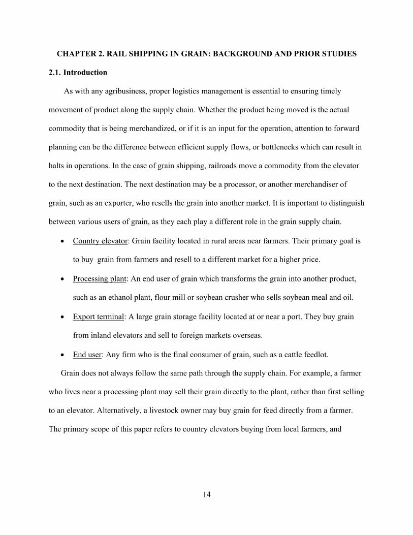
As with any agribusiness, proper logistics management is essential to ensuring timely
movement of product along the supply chain. Whether the product being moved is the actual
commodity that is being merchandized, or if it is an input for the operation, attention to forward
planning can be the difference between efficient supply flows, or bottlenecks which can result in
halts in operations. In the case of grain shipping, railroads move a commodity from the elevator
to the next destination. The next destination may be a processor, or another merchandiser of
grain, such as an exporter, who resells the grain into another market. It is important to distinguish
between various users of grain, as they each play a different role in the grain supply chain.
• Country elevator: Grain facility located in rural areas near farmers. Their primary goal is
to buy grain from farmers and resell to a different market for a higher price.
• Processing plant: An end user of grain which transforms the grain into another product,
such as an ethanol plant, flour mill or soybean crusher who sells soybean meal and oil.
• Export terminal: A large grain storage facility located at or near a port. They buy grain
from inland elevators and sell to foreign markets overseas.
• End user: Any firm who is the final consumer of grain, such as a cattle feedlot.
Grain does not always follow the same path through the supply chain. For example, a farmer
who lives near a processing plant may sell their grain directly to the plant, rather than first selling
to an elevator. Alternatively, a livestock owner may buy grain for feed directly from a farmer.
The primary scope of this paper refers to country elevators buying from local farmers, and

15
shipping to an export terminal via railroad, as shown in Figure 2.1. Specific markets are referred
to in the description of data section.
In order to ensure farmers are able to sell their grain when they want, and elevators are
able to ship grain when needed, transportation is key to facilitating grain flow. If elevators were
able to simply order railcars when they are needed and at a stable shipping price with guaranteed
placement time, there would be no need for managers to plan their shipping needs in advance.
However, this is clearly not the case. The fact that numerous factors impacting shipping demand
are random, including basis, shipping costs, and car placement, requires shippers to strategically
plan out their shipping demands based on forecasted levels of grain supply and demand.
Just as grain prices fluctuate, the cost of shipping changes daily. Not only are railcar
prices uncertain, the probability that railcars are placed when needed by the elevator changes
over time as well. Another source of uncertainty lies in the fact that elevators cannot predict the
amount of grain that farmers deliver in a given day with 100% accuracy. This means that not
only are shipping costs uncertain, but actual inventory levels are unknown to some degree as
well. These factors, along with many other sources of risk, require elevator managers to carefully
plan out their railcar ordering strategy.
Farmer CountryElevator
CountryElevator
ExportTerminal
ProcessingPlantProcessing
Plant
ExportTerminal
ForeignCountry
EndUser
Figure 2.1. Typical Flow of Grain Through the Supply Chain

16
In response, railroads typically offer an assortment of service mechanisms that give the
shipper various degrees of managerial flexibility in the service. These service mechanisms may
provide guarantees, such as offering guaranteed service for a longer timeframe at a locked-in
rate, or flexibility, such as the option to sell any unused railcars that were previously contracted
to the elevator. Understanding each of these various contracts and pricing mechanisms offered by
railroads to shippers is essential for elevators in making future plans that best match their
shipping needs.
This chapter aims to provide an overview of the development of railroad service
mechanisms, and the key features of the current major railroad service options. Prior studies on
topics related to railroad pricing mechanisms and supply chain management are then highlighted.
2.2. Evolution of Rail Pricing and Service Mechanisms
Although the federal government has regulated the railroad industry since 1887, it was
not until the 1980s that policies were enacted that helped shape the rail market into that which
we see today (Hanson, Baumel, & Schnell 1989). Prior to the 1980s, the primary mechanism for
establishing rates was posted-price tariffs which were allocated on a first-come-first-served basis
(Wilson & Dahl 2005). Under this mechanism, each origin/destination combination was assigned
a tariff rate. During this timeframe, railroads were highly regulated by the government and tariffs
rarely changed. With the first-come-first-served allocation mechanism, shippers applied for cars
as needed, but there was no tool to ensure timely car placement. This created issues during
periods of high shipping demand since cars were allocated to those that applied first, rather than
those that valued service the most. Also, there were no mechanisms in place that forward
contracted freight service.

17
These inefficient pricing mechanisms led to poor returns for railroad carriers, and forced
some into bankruptcy. With the goal of improving flexibility in pricing, the government passed
the Staggers Rail Act (SRA) in 1980. The SRA provided deregulation necessary for railroads to
have more power in establishing rates as markets saw fit and utilized confidential contracts,
which were the precursor to service guarantees (Hanson 1989 & Wilson 2005). These contracts
allowed railroads to make forward service guarantees in various forms to grain shippers.
Without any cancellation penalties being imposed on these contracts, many elevators
placed “phantom orders” just in case they would need grain in the future. By placing car orders
in excess of their actual shipping needs, elevators had a better chance of receiving service since
big orders were prioritized. The shippers could then cancel the unneeded cars and keep the ones
they needed. Not surprisingly, these phantom orders led to an inefficient allocation of cars
(Wilson & Dahl 2005).
This led to the Certificate of Transportation (COT) program created by BNSF (BN at the
time) in 1988 which had some important features including forward contracting, auction
allocation system, guaranteeing placement, and transferability (Wilson & Dahl 2005). The ability
to transfer service to another shipper led to the secondary market that we see today (Wilson &
Dahl 2011). Under the COT program, forward shipping guarantees were offered that provided
bilateral penalties for each party upon default of agreed terms. Although BNSF was the first to
adopt such a strategy, other major Class I railroads such as Canadian Pacific, Union Pacific,
CSX, and others followed with similar auction-based, and car guarantee programs (Wilson,
Priewe, & Dahl 1998).
Under the auction system, shippers placed bids to receive access to cars. In essence, the
shippers were then bidding on or valuing the added benefits of the COT program, such as

18
guaranteeing placement, forward pricing, and transferability, all of which are factors that reduce
overall risk for the shipper. This also helped ensure efficient allocation during times of shipping
surplus or shortage, since supply and demand factors would be reflected in the bids. Creating an
auction-based system implied better economic efficiency, since cars were allocated to the
shippers that valued them the most, rather than who applied first. Thus, the total shipping rate
was then the tariff rate plus the premium that was bid. Although it is possible for a bidder to
place a negative bid, i.e., a bid less than the tariff rate, the railroad has no incentive to accept
such an offer as they are the primary service holder (Sparger & Prater 2013).
The other major component of the COT program is the transferability of these
instruments. These instruments are not specific to a particular origin, destination, or shipper,
which implies that the owner of these contracts can transfer the instrument to another shipper. If
a given elevator owns a COT and does not need all of the cars that would be arriving in a given
month, the contract gives them the ability to sell the trip to another shipper. This transferability
component is what led to the creation of the secondary market. This concept lays the groundwork
for this paper and is discussed in more detail later in the chapter.
The bilateral penalties were also important since shippers would now have to pay for cars
that were ordered and then cancelled, which increased allocation efficiency. The cancellation
penalties were originally paid out of pre-payment funds that were provided to the carrier by
shipper upon winning the auction. Also, the instruments had provisions that required the railroad
to pay a penalty when cars were not delivered to shipping origins on time. In the early 1990’s,
railroads started offering long-term shipping instruments (1-3 years). Under this system, grain
companies owned cars that they would lease to the carrier and in exchange, receive a number of
guaranteed loadings each month.

19
Since its inception in 1988, the COT program offered by BNSF has undergone many
changes to the specific features and terms offered. However, the general idea of having forward
contracted freight, auction mechanisms, bilateral penalties, and transferability is still commonly
used in freight. Other railroad carriers have since offered similar programs including the Grain
Car Allocation System (GCAS) offered by Union Pacific (Wilson & Dahl 2005). The general
goals of each of these programs are to efficiently allocate cars among shippers and provide
mechanisms for risk management.
2.3. Current Pricing and Service Mechanisms
In order to understand the optionality involved in rail markets, it is important to
understand the current pricing mechanisms. Different pricing mechanisms involve different
forms of optionality, depending on the type of contract offered. Whereas some contracts may
offer guarantees of service for a period of time, others may offer price locks, or both. Various
terms and conditions in each of these mechanisms provide alternative forms of managerial
flexibility. Although specific mechanisms differ from carrier to carrier, there are some common
characteristics. For example, most large carriers, including BNSF and Union Pacific, offer both
short-term and long-term service contracts. The short-term contracts may only be for a small
number of cars and one trip, whereas the long-term contracts provide a larger number of cars for
service throughout the whole year at a specified price.
2.3.1. Primary vs. Secondary Markets in General
It is important to understand the difference between the primary and secondary market
when discussing rail markets and their functionality. The primary market, although with some
variation firm to firm, is the initial allocation of trains in which shippers bid for rights to utilize a
specified number of cars for a certain time period forward. Carriers may allocate cars on a first-

20
come, first-served basis, a lottery, or in an auction. The winners of each car offering are allocated
contracts for service which specify elements such as forward order period, rate level (tariff), and
number of cars per month (Wilson & Dahl 2005).
One of the important features of these contracts is their transferability, which is the
foundation for the secondary market. This gives the owner of the contract the right to sell a
number of cars during a given month to another shipper that is quoted as a premium or discount
on the tariff rate. This is important to shippers due to the fact that there is large variability in
shipping demand month-to-month due to intra-seasonal supply and demand levels (Wilson &
Dahl 2011 & 2005). This variability creates problems if an elevator has a locked-in, constant
supply of railcars to fill and ship out each month, since there would be months when you want to
ship more or less than your allocation of cars allows. So, the primary owner of a contract may be
able to sell one or more trips to another shipper, while still retaining the rights to that train
afterwards. This mechanism, combined with the primary market, efficiently provides shippers
railcar placement, rail rates, and the option to transfer these cars as a means to mitigate risk.
Although the topic of the effects of auctions and secondary markets has been covered in many
studies, there is limited research done on valuing these mechanisms, and even less so with real
options methodology.
2.3.2. Mechanisms Relevant to This Study
Since there are seven Class 1 railroad carriers within the U.S. along with a number of
small regional carriers, and each one has their own specific systems for car pricing and
allocation, only one system is used in this model since it’d be impossible to include the elements
from every carrier. The BNSF business model from shipping ag products is selected for a few
reasons. First, they are the largest carrier of ag products, and therefore represent the largest share

21
of individuals within the industry. Also, their allocation mechanisms facilitate a transparent
secondary market, and the bids are therefore a good reflection of market conditions. Lastly, the
elevators selected for this analysis are on BNSF rail lines. There are some terms and definitions
regarding these mechanisms that should be specified. As listed in the BNSF 4090-A rulebook:
• “Monthly Grain Single: A COT order of one (1) covered hopper car, purchased for
one (1) Shipping Period for one (1) month.
• Monthly Grain Unit: A COT order for twenty-four (24) covered hopper cars,
purchased for one (1) Shipping Period for one (1) month.
• Yearlong Grain Single: A COT order of one (1) covered hopper car, purchased for
one (1) Shipping Period per month for twelve (12) consecutive months as offered.
• Yearlong Grain Unit: A group of twenty-four (24) covered hopper cars, purchased
for one (1) Shipping Period per month for twelve (12), twenty-four (24) or thirty
-six (36) consecutive months as offered by BNSF.
• Shuttle: a full complement of covered hopper equipment (100-120 cars) with dedicated
locomotives in dedicated service for a specific period of time, which moves from a single
origin facility to a single destination facility.”
BNSF currently offers three car ordering programs to their customers; lottery cars,
Certificates of Transport (COTs) and the shuttle program. Table 2.1 lists the details of each of
these programs, and the relevant terms are discussed further below. The secondary market
mechanisms are also listed for comparison. Although BNSF allows its cars to be traded on the
secondary market, they do not participate directly. All rules within the secondary market are
privately negotiated between buyer and seller, and regulation and arbitration is provided by the
National Grain and Feed Association.

22 22
Table 2.1. BNSF Car Ordering Programs (bnsf.com)
Feature Non COT Units and
Singles (Lottery Cars)
Certificate of Transport (COTS) Pulse COTs Shuttle Program Secondary
Market Pricing -Tariff Lottery program
Single car: <15 cars Units: 24-54 cars -General Tariff program -No prepayment
-Auction system. Can be for Singles, Units, or Destination Efficiency Trains (110 cars) -Prepayment of $200/car plus premium, as a performance bond. $200 is then subtracted from total freight bill
-Price is tariff only. -No prepayment
-Weekly auctions, tariff can change each month. Winner pays bid to BNSF, rarely below tariff
-Buyers and sellers post bids/asks through a third party broker. Bid/ask can be positive or negative. Effective tariff is the rate at time of shipment
Allocation through time
-Single trip commitments -Can be either monthly (one shipment) or 12 or more monthly consecutive commitments. Priority given to bids of longer duration
-BNSF publishes daily offers for single car, one-time trips in a specified future delivery period
-Usually yearlong commitments
-Daily bid/ask sheets published and distributed by broker. Service is usually for one trip only
Allocation to Shippers
-Lotteries held each of the first 3 weeks of each month
-Weekly auctions: -Monday – DET’s -Tuesday–Monthly Units, -Wed. –Yearlong Units, -Thursday – Monthly Singles, Yearlong Singles
-First come, first served basis
-Weekly auctions each Wednesday – variable depending on market conditions
-Buyer (seller) indicates acceptance of offer (bid) through broker.
Window for Delivery
-Three 10-day periods of each month in the future
-Three 10-day periods/month in the future
-Three 10-day periods of each month in the future
-First placement is a 10-day period of the given month, after which placement is dictated by velocity
-Can be any period, usually 10-15 day window

23 23
Table. 2.1. BNSF Car Ordering Programs (bnsf.com) (continued)
Feature Non COT Units and
Singles (Lottery Cars)
Certificate of Transport (COTS) Pulse COTs Shuttle Program Secondary
Market
Specification of Want Date
-Roughly 30 days after lottery, -Customer specifies window -BNSF decides specific date
-Up to 30 days prior to shipping period. Request any date within shipping period
-Up to 30 days prior to shipping period. Request any date within shipping period.
-First shuttle order must be placed at least 10 days in advance of startup period
-Indicated at time of bid/offer
Cancellation -$100/car unless order remains unfilled by end of placement period -General tariff cars cancelled 30 days after last day of placement period
-$200/car/trip ($160 cancellation + $40 pre-pay forfeiture) for Yearlong Grain Units and Yearlong Grain Singles
-$250/car if cancelled between car order placement and last day of shipping period -$200/car for cars that are not given a specified want date prior to shipping period
-$200/car per shipment period -If a shuttle is cancelled, all remaining trips on the shuttle train are cancelled
-Negotiable between primary owner and buyer
Transfer Among Shippers
-No -Through secondary market
-Yes, but not organized by BNSF. Shippers may arrange transfers among themselves
-Through secondary market
-Resell in secondary market
Transfer. Among Origins
-Yes, upon BNSF approval - N/A - N/A -Yes, but $1,000 per train per trip IF specified after train leaves prior destination
-No
Loading Incentive
-No -Available for DET if four unit trains combined but no loading incentive
-No -Origin Efficiency Payment -Release <15 hours: $100/car -Release <10 hours: $150/car
-Yes, same as primary owner. OEP payment goes to the loading facility

24 24
Table 2.1. BNSF Car Ordering Programs (bnsf.com) (continued)
Feature Non COT Units and
Singles (Lottery Cars)
Certificate of Transport (COTS) Pulse COTs Shuttle Program Secondary
Market
Demurrage -$75/car/day after 24 hours, debit/credit system
-$75/car/day for singles after 24 hours $600/hour/train for units after 24 hours
-Standard demurrage, $75/day after 24 hours
-After 24 hours, $600/hour/train After 48 hours, $1,000/hour/train
-Standard demurrage
Guaranteed? -None -If order placed more than 10 days prior to start date. If placed 1-9 days before, cars are honored but not guaranteed placement. -If guaranteed cars are 15 days late after want date, BNSF pays max. $200/car to shipper (Non-Delivery Payment, cars still honored), or shipper can cancel.
-If order placed more than 10 days prior to start date. If placed 1-9 days before, cars are honored but not guaranteed placement. -If guaranteed cars are 15 days late after want date, BNSF pays max. $200/car to shipper (Non-Delivery Payment, cars still honored), or shipper can cancel.
-No, but if < 5 trips/month per 61-day period, shipper can cancel trip for free at BNSF discretion
-Yes. If disputes or late cars cannot be settled between parties, NGFA handles arbitration
Contract Specs.
-Date and time -Name of party -Name of person receiving request -Kind and size of cars wanted -Number of cars wanted -Date wanted -Commodity to be loaded -Destination and route
-Car number(s) -Origin -Consignor -Destination -Consignee -Route -Commodity -Other terms
-Car number(s) -Origin -Consignor -Destination -Consignee -Route -Commodity -Other terms
-Car number(s) -Origin -Consignor -Destination -Consignee -Route -Commodity -Other terms
-Date of contract -Quantity -Kind of grade of grain -Price or pricing method -Type of inspection -Type of weights -Applicable trade rules -Transportation specs -Payment terms -Other terms

25
2.3.3. BNSF Shuttle Program
Car ordering programs that are specifically used for this analysis are the shuttle program
and secondary car markets. The reason for this is that shuttles, and shuttles bought and sold
through the secondary market now represent a majority of all ag commodity railroad traffic
(industry source). Therefore, by evaluating these markets, the model best represents current
market conditions and strategies used by industry participants. It should also be noted that these
programs change on a year-to-year basis, but the main concepts usually remain the same.
Throughout the marketing year, BNSF is in constant communication with grain handlers in
regards to upgrades and tweaks that can be made to the programs in order to ensure that the
contract mechanisms are mutually beneficial for the carrier and the needs of the shippers. The
programs evaluated in this study are current as of November, 2016.
Although the exact definition of a train shuttle varies from carrier to carrier, the idea
behind the BNSF program is that a shipper bids on 100-120 car service that is forward contracted
at a locked in rate. When BNSF holds an auction for a certain number of cars, shippers place bids
that are interpreted as premiums to secure cars. This premium does not include the tariff rate that
is paid each time a shipment is made. For example, if a shipper places a winning bid of $20,000,
they make a one-time payment to BNSF of the full $20,000. The actual per-trip shipping costs
(tariff) are paid at the time of shipment. The exact schedule of auctions is not set, and fluctuates
based on BNSF’s inventory of railcars and the demand in the market. The duration of these
contracts is usually one year. This means that shippers must forecast their estimated shipping
demand for the upcoming year and bid accordingly. An advantage that the shuttle program offers
is a locked in shipping rate. The owner of the shuttle contract has the option to lock in either the
tariff rate at the time of bidding, or the rate during the first shipment.

26
As briefly mentioned earlier, although the shuttle program reduces price risk for owners,
there remains quantity risk. In the shuttle program, the train is meant to be in constant use,
running from origin to destination repetitively. Rather than BNSF specifying that the shuttle
owner gets a certain amount of trips per month, the quantity depends on railroad performance, or
velocity. When railroad traffic is low, and everything is running smoothly, a shuttle owner may
have to fill four trains in a given month. When performance is weakened due to factors such as
heavy traffic or inclement weather, a shuttle may only make two trips in a month. This is a very
important point when it comes to a logistic manager planning out freight needs. Not only do they
have to estimate how many cars they need, they have to estimate how many cars they will
receive based on railroad performance, and is therefore a random, or stochastic variable in their
logistic planning models. Historical performance of BNSF shuttles is shown in Figure 2.2.
Figure 2.2. BNSF Historical Performance (bnsf.com)
0.00.20.40.60.81.01.21.41.61.82.02.22.42.62.83.03.23.43.63.84.0
Jan-
11
Apr
-11
Jul-1
1
Oct
-11
Jan-
12
Apr
-12
Jul-1
2
Oct
-12
Jan-
13
Apr
-13
Jul-1
3
Oct
-13
Jan-
14
Apr
-14
Jul-1
4
Oct
-14
Jan-
15
Apr
-15
Jul-1
5
Oct
-15
Jan-
16
Apr
-16
Jul-1
6
Oct
-16
Trip
s per
Mon
th
BNSF Ag Fleet TPM History

27
Another very important aspect of the shuttle program, and the key component of this
study, is the transferability of the service. This can also be interpreted as an option given to the
owner when they do not need the train. If a shuttle contract owner finds that they do not need all
of the cars coming to them in a given month, they essentially have three options. They can either
cancel the cars for $200/car/remaining trip, sell them into the secondary market, or source grain
in order to use the cars, in what we refer to as a “forced” shipment. There is also the option of
letting the cars sit idle, but this incurs significant demurrage costs, and is not considered a viable
alternative for this study. Since it is not possible to cancel just one or two trips, or essentially
pause the shuttle, timing plays a large role in deciding whether to cancel cars or sell into the
secondary market (industry source). If secondary market values are trading at a discount, or
negative rate, the shuttle owner who does not need all of the cars must decide whether to pay the
cancellation fees and forfeit the rest of the trips, or to sell the cars for a loss and retain
ownership. If there are still many months left on the shuttle contract, the owner may be willing to
sell cars at a large loss (less than -$200/car) in the short term in order to retain ownership in
hopes that shipping demand and/or secondary market prices rally in the distant months. If there is
only one month left on the shuttle, or only a couple of trips, there is no incentive for the owner to
sell the remaining trips for less than $200 below tariff, when they can just cancel them for
$200/car/remaining trip. The cancellation economics behind a shuttle contract are very dynamic
and involve many variables. The only time a shuttle owner may cancel a single trip, is if they
receive less than five trips in 61-day period, but this is at the discretion of BNSF and does not
happen very often.
Since the main point of the shuttle program is to efficiently allocate railcars and move
grain, BNSF wants cars to be moving rather than sitting in a rail yard or at an elevator. In order

28
to encourage this, BNSF began charging demurrage, and offering Origin Efficiency Payments
(OEP). Demurrage is a penalty that elevators must pay to BNSF if cars sit on their tracks for
more than 24 hours. If cars are released under 15 hours, the elevator receives an OEP of
$100/car, and this value increase to $150 if released in 10 hours or less.
2.3.4. Secondary Market
Although the secondary market is similar in some ways to the primary market, there are
some key differences that managers must take into account. Instead of an auction-based car
allocation system, a bid-offer system is used (Crabb, John). These bids and offers are published
either through a third party broker, such as TradeWest, or directly from the shuttle owner (e.g.,
CHS, ADM, etc.). Since each elevator can only ship with certain carriers, there is a separate
secondary market for each carrier that allows such a program. These offers are published daily
and come in a variety of forms. All bids and offers are quoted as a premium or discount in
relation to tariff. For example, if an elevator bought secondary cars for $100/car/trip, they must
pay $100/car/trip to the seller, and the tariff rate to BNSF. Bids and offers are usually for one trip
only, but can be for multiple forward trips as well, usually out to a year. For example, the offer
could specify two trains per month for the next five months at a certain price. The bid or offer
also lists a specific window for delivery. These windows are usually ten days, and are either first,
second, or third period of each month. If it lists a fifteen-day period, it is for either the first or last
half of the month. If a buyer of secondary market service decides that they do not need the cars,
they can either resell in the secondary market, or cancel for a fee. The secondary buyer usually
does not have free reign over the cars, though, and resale and cancellation must be negotiated
with the seller. Similar to the primary market, secondary buyers can be either charged
demurrage, or receive OEP. Payment under these programs would be from (to) the secondary

29
buyer to (from) BNSF. Figure 2.3 shows part of the bid/offer sheet that TradeWest Brokerage
Co. sends out each day. It is showing that, at the time, there are shippers looking to buy cars for
$115/car, and sell cars for $145 for shipment anytime in January.
One of the important and relevant aspects of the secondary market is the fact that car
placement within the specified time window is guaranteed by the seller. This a big difference
from the primary market, where this guarantee does not exist. If a secondary seller is unable to
get cars to the secondary buyer’s location within the window listed in the contract, the seller is
considered in breach of contract. Under this situation, the buyer has the option to either accept
the late cars and resume business as usual, or require that they receive cars from another source.
The buyer could either buy cars elsewhere and force the original secondary seller to pay any
price differentials, or have the seller furnish cars from another train that they control. Either way,
the solution to late cars is usually negotiated between the buyer and seller. If a resolution cannot
be reached, the case is handled by the NGFA.
2.4. Central Freight Desk System
The separation between primary and secondary markets is not always black and white as
far as the terminology. While a few small grain companies do buy shuttle contracts, a majority of
Figure 2.3. Bid/Offer Sheet for Secondary Market (Courtesy of TradeWest Brokerage Co.)

30
the current shuttle contracts are owned by a few of the largest shippers (industry source from
ADM). Rather than each individual elevator buying shuttles from BNSF, a grain company who
owns many elevators buys a large pool of shuttles that is managed from central freight desk. A
shuttle train almost never sticks with one elevator, but rather sticks with one grain company or
operator and trips are allocated between elevators as needed. As long as the train is notified
before it reaches a destination, the next origin can be any location at the choice of the contract
owner.
The freight desk, who controls and manages all of the shuttles that a grain company
owns, works with country elevators, both owned and not-owned, to sell shuttle trains for either
single-trip or multiple-trip commitments. Due to this “freight desk” system, the line between
primary and secondary markets is not always clear. Some freight managers consider the primary
market as strictly transactions between them and BNSF (industry source from CHS). Some
freight managers who work with a regular book of country elevators (some owned by the
company and some not) consider transactions between them and the country elevators as primary
market transactions. If the freight manager sells a train to a non-regular customer, they may
consider this to be a secondary market transaction. The country elevator that buys the train
usually has the option to either resell or cancel the trip. However, this is at the discretion of the
freight desk operator.
According to at least one large U.S. grain company, a freight manager typically sells their
shuttles to elevators for $25-$50/car/trip over the premium that they paid BNSF for the cars. The
freight desk operator is assuming all risk and liability in regards to the cars being placed on time.
In situations where cars are not able to be placed on time, the freight operator and country
elevator are in communication to determine the solution, and a resolution is usually achieved

31
before arbitration from the NGFA is required. Whereas, if the elevator were to buy cars straight
from BNSF, they would be at risk of late car placement.
Although the exact definitions of primary and secondary markets are not standardized in
practice, in the interest of clarity we must establish some language for this study. The primary
market strictly refers to transactions between BNSF and the owner of the shuttle contract.
Secondary market transactions refer to sales between either: 1) freight desk operators and any
customer (country elevator), or 2) country elevators and another country elevator. Further clarity
is provided as needed. A visual of this freight desk system is represented in Figure 2.4. It should
be noted that the figure is purely hypothetical, and does not represent the business of any specific
company.
Figure 2.4. Freight Desk System Flowchart

32
2.5. Previous Studies on Rail Pricing Mechanisms
The last section of this chapter reviews the current literature on rail shipping in grain
markets. The specific subjects reviewed are the impacts of rail rates on basis, railcar allocation
mechanism design & pricing, and rail pricing and logistical supply chain management.
2.5.1. Impact of Rail Rates on Grain Shippers and Producers
Many different researchers have studied the history and effects that the rail policy
changes of the 1980s had on the grain market. Before railroads became deregulated, Martin
(1979) argued that the rail rate structure of the time was based on “value of service,” rather than
“cost of service.” This structure was concluded to operate to the disadvantage of society.
Hanson, Baumel, and Schnell (1989) argued that it was excessively tight government regulation
during that first century that led to the bankruptcy of many large railroads. These regulations
made it difficult for railroads to have the flexibility needed to adapt to various changing market
demand conditions and the freedom to drop business units that were not performing, which led to
widespread failure. Vachal, Bitzan, VanWechal, and Vinje (2006) also studied the effects of rail
deregulation and found that both grain shippers and producers benefit from the decreased rail
rates. However, producers in areas with more inter and intra-modal competition benefit more
than those in less competitive areas. They summed up the importance of shipping prices to
farmers with the statement, “Rail rates are a key determinant in grain market viability and
producer profitability in these rail dominated markets.” The market structure of the railroad
industry and its impact on rates has also been studied. Winston, Maheshri, & Dennis (2011)
found that the impact of the mergers of large railroad companies have no long-run impact on
grain transportation prices and consumer welfare.

33
A number of studies have been conducted with the goal of examining the causal
relationship between rail prices and basis levels/prices to producers. Wilson & Dahl (2011)
found that basis has become more volatile over time, and is impacted by factors such as shipping
costs, ocean rate spreads, export sales, railroad performance, and others. Their results further
validated some previous findings about increases in basis volatility and the importance of export
sales’ effect on basis. On the other hand, their results found performance in rail car shipments to
be less of a determining factor in basis whereas other studies found the impact to be much
greater.
Rail service disruptions caused by increased traffic from competing commodities, such as
oil, have been reported to have impacts on elevator prices, and have been a popular research
topic. Villegas (2016) concluded that oil traffic, among other factors, is a determinant of wheat
basis, and that this relationship is stronger in upper Midwest states, like North Dakota. The latest
major example of this phenomena in the Upper Midwest was during the 2013-2014 marketing
year when increased rail demand from oil and coal led to disruptions in grain shipping. Unable to
move their inventory, shippers were forced to bid less aggressively for grain. This led to multiple
studies on the topic to quantify the impact this had on producers. A study done by Frayne Olson
(2014) for Sen. Heidi Heitkamp estimated that rail disruptions caused an aggregate loss to
farmers statewide of $66.6 million, or a little bit over $2,000 per farm. This study did not
necessarily analyze a direct relation between railroad price, performance, and basis. Rather it
assumed that basis would be the same as an analogue year, and then made derivations. In a report
for the Minnesota Department of Agriculture, Usset (2014) used similar methods to estimate the
impact of the 2013-2014 rail disruptions on Minnesota producers. Comparing 2014 to years with
similar grain supply/demand levels, he estimated that farmers lost 40 cents/bushel on soybeans,

34
30 cents on corn, and 41 cents on hard red spring wheat. Another study by the Agricultural
Marketing Service of the USDA (2015) estimated the losses to be three percent of all farm cash
receipts, but acknowledged the difficulty of pinpointing the exact cause of these losses. In
another resulting study for the American Farm Bureau Federation, Kub (2015), further reviewed
the 2013/2014 situation, but also argued that increasing infrastructure of truck, rail, barge, or
pipeline transportation would reduce congestion of grain flow.
2.5.2. Railcar Allocation Mechanism Design & Pricing
After the Staggers Rail Act, researchers have conducted studies on the specific contract
mechanisms offered by carriers, and how they impact car ordering strategies by shippers. In their
findings, Hanson et al. (1989) concluded that these guarantee contracts that were “origin”
contracts (contracts between grain shippers and railroads) had a large impact on local wheat bids
to farmers and “destination” contracts (contracts between non-elevator grain buyers and
railroads) had large impacts on corn and soybean bids. One limitation of their model was that it
assumed the grain bought from farmers was immediately resold to another user, which does not
account for storage decisions. In a similar study, Hanson, Baumhover, & Baumel (1990) found
that transportation factors such as contract terms, mileage allowances, and mode all have
significant impacts on handling margins for grain elevators.
Similar to Hanson (1989), Wilson & Dahl (2005) analyzed the impacts that guaranteeing
mechanisms have on the grain industry. Much of the previous studies had concluded that
auctions are effective in car allocation. Although the authors agreed with this, they were among
the first to point out some problems with the system and what the market did to overcome them.
They highlighted the fact that each shipper has unique costs facing them and therefore each

35
employs different bidding strategies, and also the importance that informational advantages have
in competition between elevators of the same region.
The main study that provides framework for this analysis is that of a master’s thesis by
Lee (1999). While the specific model structure and parameters differ from those in this study, the
Lee analysis was the first to incorporate real option analysis into valuing rail contracts for grain
shippers. At the time, BNSF offered a contract that had three main components: 1) it allowed for
transferability of cars into the secondary market, 2) a better probability of cars showing up on
time relative to the general service contracts, and 3) required a deposit of $300/car. The Lee
model calculated the summation of payoffs from these three components, and interpreted the
result as the total contract value. Real option analysis was utilized to value the transferability
component. The only component of these contracts that is still present in today’s shuttle
contracts is the transferability, which is interpreted as an option value and is the focus of this
study. Lee found this transferability to be worth $3.21 per car, and that volatility of shipping
demand and secondary market prices had a large, positive impact on this option value.
Our study incorporates more modernized modelling techniques, and more extensive data
sources in order to account for differences in rail contract structure, and provide refined results
with fewer assumptions. For example, the Lee model uses farmer deliveries as a proxy for
monthly shipping demand. Rather, this model includes a simulated rail shipping demand
schedule derived from farmer deliveries, returns to storage, and other key variables. Another key
difference is that the payoff structure of the Lee model allows for the possibility of a negative
value of the transferability, or a negative option value. Since the theory on option pricing does
not typically allow for negative values, this problem is addressed and accounted for in our

36
model. Also, whereas the Lee model results are interpreted as the total contract value, the results
of this model are interpreted as just one component of the total contract value.
Wilson, Priewe, and Dahl (1998) conducted a comprehensive strategic analysis of various
car ordering strategies for a grain shipper based on non-guaranteed, short-term, and long-term
guaranteed service. Results indicated that, at the time, strategies using short-term car guarantees
provided for larger payoffs, but also more risk exposure. They also concluded that variability in
farmer grain deliveries has a significant impact on the shipper’s bottom line. These results are
important to note, since they demonstrate that contracts that offer a long-term car guarantee help
reduce risk for an elevator, and therefore may have more value than a short-term contract.
2.5.3. Rail Pricing and Logistical Supply Chain Management
Other studies on railroad logistics have focused on how the prices, mechanisms, and
strategies implemented by shippers affect the grain supply chain. Wilson, Carlson, and Dahl
(2004) corroborated other studies by demonstrating that shippers who utilize forward freight are
provided with better service reliability, and that managers need to take rail performance into
account when making car ordering decisions. According to the study, “Results from these
simulations demonstrate that demurrage costs can be reduced by adopting the anticipatory
strategy. In fact, ordering cars naively and ignoring railroad performance, results in higher costs.
Hyland, Mahmassani, and Mjahed (2016) conducted a study to demonstrate the effects that
switching from conventional rail service to shuttle have on travel time, cost, and capacity of
railroads. One unique part of their model is that it included negative impacts incurred to
upstream supply chain participants due to shuttle implementation. These include longer trucking
distances between farms and elevators, and longer storage times at elevators, both stemming
from the fact that shuttle programs help give rise to elevator consolidation. Results indicated that

37
shuttle service transports grain faster, cheaper, and increases rail capacity compared to
conventional service. However, one of the assumptions, among many others, is that both shuttle
and conventional railcars show up to the elevator as soon as it accumulates enough grain to fill a
train. This ignores the facts that rail performance differs between shuttle and non-shuttle
programs, and that elevators frequently store grain for at least some period of time. A similar
study by Ndembe (2015) also found that increased use of shuttle trains in North Dakota, along
with intermodal competition, lead to reductions in rail rates.
Studies have also analyzed the relationship of demand for rail shipment with various
explanatory variables. Babcock & Gayle (2014) used a two-region spatial equilibrium model to
find that crop production and barge rates have a positive impact demand for rail shipment, while
rail prices have a negative relationship with rail demand. In a similar study on rail demand,
Prater, et al. (2013) analyzed the decrease in the share of grain and oilseed harvest being moved
by rail. They found that increased ethanol production, biodiesel production, and concentration of
animal feeding are three of the most significant explanatory variables.
In study comparing spatial differences in rail rates, Babcock, McKamey, and Gayle
(2014) compared wheat rates per ton-mile in states with inter-modal competition (Kansas) to
those in captive markets (North Dakota and Montana). Results indicated that North Dakota has
the highest rail rates for wheat, whereas there is little difference between rates in Kansas and
Montana.
2.6. Summary
In conclusion, this chapter provides an overview of the current shipping mechanisms
available, and the prior studies done on grain shipping. There are many different sources of risk
facing grain shippers, and each provides a unique challenge. Of these, certain sources of risk are

38
easier to mitigate than others. Grain prices can be mostly hedged with futures, and grain quantity
can be partially mitigated with the use of forward contracts. Risk in rail shipment of grain is
more difficult to manage since there is no derivative market for hedging. Users of primary shuttle
instruments can lock in shipping rates, but the quantity of rail cars received is subject to rail
performance. Users of secondary rail shuttles are guaranteed placement within a window of time,
but they are subject to price risk every time they make a purchase, unless they negotiate a
forward contract with the seller.
The current rail shipping mechanisms available to elevators each offer unique flexibility,
or optionality. This optionality is essential considering the dynamic nature of grain shipping. The
main option available to a user of primary cars, and the focus of this study, is the ability to
transfer, or sell cars into the secondary market. This transferability comes into consideration
when a shipper either cannot fill all of the cars coming to them, or finds that it is more profitable
to sell rail cars rather than sell grain. In order to plan logistic needs, shippers must evaluate the
various mechanisms available to them. Since some rail contracts offer this transferability and
some do not, a shipper must know how much of a premium to pay for a contract that includes
this option versus one that does not.
While there have been many studies done on rail shipping in grain, the majority of the
existing literature analyzes relationships between factors such as rail prices, rail demand, basis
levels, and regulation policy. Little has been done on topics of shipping strategy or valuation of
alternative contracts available to shippers, or to value individual options imbedded within these
contracts. This model builds on the framework of the 1999 Lee study, but has key differences as
previously referred to. Other than that of Lee, no other study in this field of grain shipping has
utilized real option analysis.

39
3 CHAPTER 3. REAL OPTION ANALYSIS: BACKGROUND AND PRIOR STUDIES
3.1. Introduction
Virtually all investment decisions, whether it is to develop an oil reserve or buy an input
for business operations such as railcars, involve risk and uncertainty. Traditional methods of
capital budgeting and valuation, such as net present value (NPV), work well in evaluating the
quantitative aspects of investments. However, there are many qualitative or strategic components
of an investment that require more creative methodologies to accurately value, such as certain
types of managerial flexibility, and this flexibility has value (Trigeorgis 1996). Real Option
Analysis (ROA) is a relatively new and evolving capital budgeting technique which aims to
quantify some of these qualitative characteristics of investments.
It is important to distinguish when the real option approach is necessary. In general, it
comes down to the level of uncertainty and flexibility involved with a decision. If there is little
uncertainty and little flexibility involved with a decision, traditional budgeting methods are more
appropriate (Amram and Kulatilaka 1999). Given the dynamic and complex nature of grain
logistics, ROA is an appropriate technique to evaluate railcar ordering and mechanisms. There
are many sources of uncertainty in railcar demand, and the decision to buy railcars and sell
excess railcars is contingent on the amount of shipping demand we have. This chapter provides
an overview of ROA in general, the specifics of the type of option used in this study, and a
summary of prior studies that have implemented ROA.
3.2. Real Option Analysis Overview
Over the past thirty years or so, ROA has developed as an alternative financial method to
evaluate capital expenditures and investments. According to Dixit and Pindyck (1994),
investments involve both quantitative features such as costs, prices, and dividends, and

40
qualitative features such as irreversibility, uncertainty, and timing. Irreversibility refers to the
fact that once an investment is undertaken, at least part of the initial outlay is a sunk cost and is
unrecoverable should the investor change their mind later on. Uncertainty is an important factor
that affects the future rewards of an investment. In nearly all investments, expected cash flows
are affected by many different factors, and the slightest change can be the difference between
positive and negative return on capital. Timing of an investment is also important as it helps to
better gauge the potential outcomes. If an investor is able to postpone an investment in order to
get more information about the future, they can reduce some (but usually not all) of the
uncertainty. The interaction of these qualitative characteristics play an integral role in
determining investment outcome, but are overlooked in traditional capital budgeting models
(Dixit and Pindyck 1994).
3.2.1. ROA vs. NPV
Real option analysis is a fairly new topic that has been gaining in popularity as a way to
evaluate a project or asset’s inherent value while taking into account variability that arises
throughout its lifespan. It is comparable to NPV and discounted-cash-flow (DCF) methods in
regards that they are both valuation tools (Turvey 2001). However, the NPV approach has some
implicit assumptions that make it a more rigid tool and weaken its connection between theory
and application. For one, it assumes that investments have a “now or never” proposition. That is,
an investment must either be taken today based on current market expectations, or never at all. In
reality, literature has shown that the ability to delay an investment can have a substantial impact
on the overall result (Dixit and Pindyck 1994). Another assumption of the NPV approach is that
cash flows are static and known beforehand with some degree of certainty (Trigeorgis 1996).
This presumption about not only static cash flows, but a static operating strategy (committing to

41
investment until the end of its expected useful life), implies that the value calculated through
NPV analysis can only be generated if all expectations about costs, sales, prices, demand, etc. are
correct.
Amram and Kulatilaka (1999) point out that in order to compensate for the static nature
of traditional investment forecasts, managers may provide a range of forecasts. Even if the
outcomes under these various forecasts are known, the decision to invest or not is still subjective
in nature. The authors also discuss managerial flexibility. As an investment takes course,
mangers are usually presented with opportunities to possibly expand, contract, or shut down a
project, among other alternatives. The contingency nature of these investment decisions shows
that they are not static, but rather dependent on outcomes from prior events. Traditional methods
of budgeting fail to take into account this managerial flexibility and the impact that it may have
on the overall return.
Real option analysis takes into account uncertainty, flexibility, and irreversibility of the
decisions that are made throughout a project’s lifespan, which is not accounted for in NPV since
NPV assumes static cash flows. Alizadah and Nomikos (2009) pointed out that ROA becomes
more important as the uncertainty in project increases since volatility is not taken into account
for using traditional NPV. Due to this fact, the actual value of a project is often understated using
NPV since there are options, either hidden or not realized, embedded within a given deal. NPV
fails to quantify the uncertainty, flexibility, and irreversibility that these additional options
provide (Turvey 2001).
3.2.2. Real Options vs. Financial Options
In the most simplified terms, real option analysis is essentially taking financial option
pricing methodology and applying it to a “real” asset. In financial derivative markets, a call

42
option is the right to purchase the underlying asset, and a put option is the right to sell. The
owner of a call option has the right, but not the obligation to purchase the underlying asset at a
specified price called the strike price. In return for the option, the owner pays a premium to the
seller. In contrast, the owner of a put option has the right, but not the obligation to sell an asset at
a given strike price, and similarly pays a premium to the seller of the option in order to obtain
this right. With traditional financial options, the underlying asset that is being bought or sold
upon exercise is either a stock on a company or a futures contract.
ROA uses same principle and applies it to physical assets. Instead of the option allowing
an owner to purchase, say, a corn futures contract, the option may allow the owner to explore a
tract of land for gold. If the soil test results are favorable, the owner of the option could exercise
their right to buy or lease the land. For example, a quarter of farmland for sale may also be
embedded with the chance to rent more of the seller’s land in the future (option to expand). This
would be treated as a call option, since it involves the right, but not the obligation to make
further investment down the road. If you make the investment, you are exercising the option, in
which case the strike price is the cost of renting the additional land (Dixit 1989).
Current option pricing theory states there are five factors that affect financial option
value; underlying stock price, strike or exercise price, time to expiration, volatility, and interest
rates. As shown in Table 3.1, these five factors can be applied to investments, and be used to
price an option on buying or selling the underlying asset or investment.

43
Table 3.1. Financial Options vs. Real Options (Trigeorgis 1996)
Option on a Stock Real Option on Investment
Current value of stock Gross PV of expected cash flows
Exercise price Investment cost
Time to expiration Time until opportunity disappears
Stock value uncertainty Project value uncertainty
Riskless interest rate Riskless interest rate
3.3. Types and Examples of Real Options
Given the vast scope of investment opportunities, there are many different types of
flexibility that may be available to a potential investor. Each investment has unique
characteristics, and therefore may incorporate different types of optionality. The following
describes some common types of real options and examples of where they can be applied.
• Growth options – Whenever early investment in a project may lead to the potential for a
future investment, this can be thought of as a growth option. The key here is that in order to
undertake the future investment, the decision maker must first take part in the initial
investment. Based on the success of the initial cash outlay, the investor has a better idea if it
is optimal to undertake the future investment. Common applications include R&D, and
strategic acquisitions. An example would be if an investor is considering purchasing a
pharmaceutical company that is developing a drug which, if approved, would take 5 years to
generate cash flow. Hence, the probability of the drug getting FDA approval may impact the
value of the pharmaceutical company today (Trigeorgis 1996).

44
• Deferment option – If an investor holds the rights to defer investment until market conditions
potentially improve in the future, this adds value to the overall investment and can be viewed
as an option (Trigeorgis 1996). This is also referred to as a postponement option, or a wait-
and-see option (Winston, 2008). An example would be a company who owns a lease to a
tract of undrilled land with oil reserves, but current oil prices make the investment to drill not
worthwhile. Or, a farmer with grain storage who has the opportunity to hold his inventory
until prices are more favorable in the future.
• Licensing option – This is common in industries that require patents and intensive R&D. In
many licensing agreements, the developer of a patent may sell the technology to a marketer.
An initial payment may be followed by additional payments that are contingent on the
success of selling the product which requires the patent. From Winston (2008): “Suppose that
during any year in which profit from a drug exceeds $50 million, we pay 20% of all returns
to the developer of the drug. What is the fair price for such a licensing agreement?”
• Option to sell/transfer/abandon – If an investment has been made, but market conditions
change over time, management may be able to abandon the investment and sell the assets at
current market value. The resale value has an impact on the initial value of the investment,
since a higher resale value adds insurance to the asset. This is common in capital-intensive
industries such as airlines and railroads (Trigeorgis 1996). For example, anyone who has ever
bought car insurance has essentially purchased a real option. In the event of a bad car
accident, the value of the vehicle drops to the salvage value. However, with insurance, you
have the option to essentially sell the car for the amount that it was covered for minus any
deductible, synonymous to a put option. The premium one pays for car insurance each month
can be thought of as a premium on a put option.

45
• Switching option – Whenever a manager has flexibility in regards to the output mix of an
operation, or the inputs needed to produce an output, this adds value to the operation. If input
prices are volatile, the ability to switch between inputs allows the manager to make cost-
effective decisions (Trigeorgis 1996). Consider a farmer who lives near many elevators vs.
one that only lives near one elevator. The famer with more markets to sell to can switch
where they deliver their grain based on who is offering the best prices. Similarly, a farmer
who can grow multiple different crops has the ability to change year-to-year output based on
which is the most profitable.
In addition to these, there are numerous other option types that may be present in any
given investment. There are also cases when multiple options are available in an investment.
These situations are referred to as compound, or sequential options. These situations require
more complex analysis since if the options interact with each other, their joint value may differ
from the sum of their separate values (Trigeorgis 1996). Also, similar to financial options, real
options can be classified as American or European. American options can be exercised at any
time before expiration during the life of the option, whereas a European option can only be
exercised at expiration (Winston 2008).
3.4. General Methods of Calculating Real Option Values
As there are many different types of real options, there are many different methods to
calculate option values. Each method or approach provides different ways to calculate a solution
for an option. The type of approach used depends on scope of the problem, and the various
flexible and uncertain components of the decision. This section gives a brief overview of the
solution methods described by Amram and Kulatilaka (1999), and the solution techniques

46
available under each method. The proceeding section then provides a more in-depth look at the
methods used in this study.
Amram and Kulatilaka (1999) present three general option solution methods: partial
differential equations (PDE), dynamic programming, and Monte Carlo simulation. “The PDE
solves a partial differential equation that equates the change in option value with the change in
the value of the tracking portfolio.” This approach is an easy and fast way to solve option values,
but cannot be used in situations with many sources of uncertainty or contingency decisions.
There are three different ways to calculate option values with the PDE approach: analytical
solutions, analytical approximations, and numerical solutions. The most widely used PDE
method to provide an analytical solution is the Black-Scholes model. The Black-Scholes model
is popular for its simplicity and risk-neutral approach. Only five inputs are needed for the Black-
Scholes model: current value of the underlying asset, cost of investment, risk-free rate of return,
time to expiration, and volatility of the underlying asset. However, due to the complex nature of
rail shipping and contingency nature of decisions, it is not appropriate for the scope of this study.
The idea behind dynamic programming is to take potential outcomes of an investment
decision while incorporating optimal future decision strategy, and discounting the values back to
the present. The most common solution technique using dynamic programming is the binomial
option approach. The binomial approach assumes that the underlying variable being analyzed
can move up or down in each period of time based on volatility and probability measures. Based
on the state of the underlying variable at each period, a decision is made based on numerical
rules in a backward recursive fashion. Dynamic programming is an attractive method for its
ability to handle complex decision structures, and offers transparency into sources of option

47
value based on intermediate values. As this study utilizes this approach, it is discussed in more
detail later.
The Monte Carlo simulation method uses stochastic processes to estimate thousands of
possible outcomes of an underlying variable. It simulates outcomes of each variable based on
input parameters and takes “draws” from a distribution of possible returns. Based on the outcome
of the underlying variable, an optimal decision is made and the payoff from the decision is
discounted back to the present time. After thousands of draws or “iterations”, the average of the
outcomes is used to determine the option value. Simulation is useful since it can be utilized with
other solving techniques, and can handle complicated decision rules. Since most options require
forward projections, simulation accounts for the fact that forecasted values rarely reflect reality
to a high degree.
3.5. Methods Relevant to this Study
This section explains the theory behind the methods that are specifically used in this
study, and links real option theory to the application of railcar shipping. The first part
demonstrates how the transferability component of a primary rail instrument can be modeled as a
put option. The next section explains the theory behind the solution method, which is the
binomial option pricing model. Then, a generic example is provided of a European real option
solution using the binomial pricing method.
3.5.1. Railcars as a Transfer Option
As a primary shuttle contract owner, one of the key components of the instrument is the
ability to transfer service into the secondary market to another shipper who is willing to pay for
the cars. In a given shipping period, if the owner of the shuttle contract finds that it is suboptimal
to utilize all of the railcars coming to them, they can sell the excess cars. Another way to say this

48
is that they have the option to abandon the cars for a salvage value. Note that it is not the contract
itself that is sold into the secondary market, but rather individual trips. Given the temporary
nature of the sale of assets, the term “transfer” is used for clarity rather than “abandon,” but the
underlying principles are the same. The only difference is that a typical abandonment option
assumes that once the sale of assets is made, the investment is over. Alternatively, with the
transferability of railcars, the owner can sell an individual trip and retain ownership of the
contract for future shipments. This means that each individual shipping period can be modeled as
a separate option. For simplicity, this study assumes a shipping period is one month. Specifically,
since a put option gives the owner the right, but not the obligation, to sell an underlying asset, an
abandonment or transfer option can be modeled as a put option (Winston 2008, Alizadeh and
Nomikos 2009).
In a financial put option, the underlying variable that determines the intrinsic value of the
option is the futures price. If the futures price drops below the strike price, the option is now “in
the money” since it has intrinsic value. The owner can then exercise their right to take a short
position at the strike price and receive the difference between the futures price and strike price. If
the futures price is above the strike price, the option to sell at the strike price has no value and
the owner’s loss is limited to the premium paid for the option. The same idea applies to rail
contracts. Instead of the underlying variable being a futures contract, the main determinant of the
option value is the level of shipping demand. If shipping demand drops below the shipping
supply, i.e. the amount of rail cars coming to the shipper, then the shipper has excess rail cars to
use up. Therefore, shipping supply is comparable to a strike or exercise price since it is the level
of shipping that triggers an excess or shortage of cars. Without the transferability, the shipper
would be forced to either use the cars anyways, or cancel the contract and pay a steep penalty.

49
Therefore, the more excess cars the shipper has, the more the transferability is worth. This is
analogous to saying that the transfer option has value, or is “in the money.” Whenever shipping
demand exceeds shipping supply, the option to transfer cars has no value since there are no
excess cars to sell. The shipper then has to either buy in cars from the secondary market to cover
the car shortage, or forgo shipping the grain. The shipper is then out only the extra money, if any,
that they paid to have the transferability option, which is the focal point of this study. If a shipper
has the hypothetical choice between a contract with and without the transferability component, it
is important to know how much of a premium they should be willing to pay for the
transferability. Figure 3.1 demonstrates the relationship between regular put options and the
transferability of railcars.
Figure 3.1. Relationship of Put Options and Railcar Transferability

50
3.5.2. StochasticBinomial Option Pricing Model
The binomial option pricing model (BOPM), first proposed by Cox, Ross, and Rubinstein
(1979), is a popular method for pricing both financial options and real options. It assumes that
the life of an option, t, can be broken down into equal discrete time periods,∆#, and the path of
the asset value follows a binomial process. During each discrete time period, the underlying asset
can either increase or decrease by an up factor, u (u > 1), or down factor, d (d < 1). u and d are
held constant throughout the length of the option. Starting with the base value of the asset, and
ending with the expiration of the option, the asset branches out into a tree that represents a series
of up or down movements based on the asset volatility, s, and risk-free interest rate, r. The
probability of an up movement is defined as p, and therefore the probability of a down
movement is (1-p).
The binomial pricing method is popular for its flexibility in a wide range of uses. It is
useful in real option analysis for its ability to incorporate changing volatility, contingent
decisions, and easy calculations. Further, the only information needed is the current asset value,
volatility, and the risk-free interest rate. It also is based on the risk-neutral approach, which
implies that the return of any asset should be the risk-free rate of interest in a risk-neutral world.
Once the current asset value, volatility, and risk-free interest rate are known, the first step
to create a binomial pricing tree is to estimate the parameters for u, d, and p, which are:
u=&'∗√(∆+) (3.1)
d=.
/ (3.2)
p=
[2(3∗∆4)56]
(856) (3.3)

51
Starting with the initial asset value, the first branch of the tree is constructed as in Figure 3.2
below.
This process is repeated until all branches are calculated, and at the end there is a set of
possible outcomes, similar to Figure 3.3 below. The number of branches depends on the length
of the option and ∆t. For example, if the time interval is one month on an option that expires in
one year, there are twelve branches. The time interval depends on user preference and there is no
set number required, but more branches provide for more robust results.
The next step is to calculate the payoff of the option at each node at expiration. The
payoff for a put and call option are as follows:
Figure 3.2. Generic One-Branch Lattice Tree
Figure 3.3. Generic Extended Lattice Tree

52
;<=># = max(B − D<, 0) (3.4)
;<GHII = max(D< − B, 0) (3.5)
where VN is the value at each expiry node, X is the strike price of the option, and SN is the price
of the underlying asset at expiration.
The final step is to discount the payoffs back to the present by a method of backward
induction. The payoff is calculated starting with the penultimate node and continued backwards
in a sequential manner. European option values at each node are calculated as:
;J = &5K∗∆L(M ∗ ;/ + 1 − M ∗ ;P) (3.6)
where ;J is the option value at each node, and ;/ and ;P are the option values of up and down
movements at Q + 1. This process is repeated until the first initial node is derived, and this value
is the final option value.
The payoff for an American option is slightly different, since the value at each node must
be compared to the possibility of early exercise, but is not used in this study.
3.6. Real Option Analysis in Prior Studies
3.6.1. Early Real Option Studies
Although financial option pricing has been studied extensively since the 1970s, it was not
until a decade or so later that real option theory started gaining popularity. McDonald and Siegel
(1985) demonstrate how option pricing theory can be applied to a firm that has the option to shut
down production if variable production costs exceed revenues. Pindyck (1988) points out that the
timing of an investment can be thought of as an option. Before an investment is made, a manager
has the option to wait or defer the investment to any point in the future. Therefore, when
investment is made, they are exercising the option to wait. Pindyck argues that this is an essential

53
component in investments with industry-specific capital since the project is most likely
irreversible.
Dixit (1989) was also one of the first to study real options as they apply to investment
decisions. He made the connection between the decisions that firms face under uncertainty and
options in that there is a certain “trigger price” where firms should enter a deal, which is similar
to a call option. Dixit argues that the cost of an investment is similar to a strike price, and making
the investment is analogous to exercising a call option. He also recognizes that, in some
situations, exercising can lead to additional options, such as abandoning the investment in the
future, which leads to a compound option, and requires deeper analysis. Kemna (1993) provides
an early collection of case studies on real options in the petroleum industry.
3.6.2. Real Option Analysis in Agriculture
Real options have been applied to many different areas of agriculture and have a virtually
unlimited number of possibilities. In an early study, Flood (1990) demonstrates how real option
pricing can be applied to the federal deposit insurance system. By setting a price floor, insurance
acts like a put option, and this model shows how option valuation can estimate the net value of
the government’s fund, or determine a theoretical insurance premium for banks. Similarly, Dahl,
Wilson, and Gustafson (1995) use real option pricing to estimate the value of credit guarantees
offered to various importing countries. This credit guarantee is similar to insurance, and can be
modeled as a put option. Results show that Canadian guarantee programs have the lowest
implicit value, while French guarantees have the highest value. In another real option study on
support programs, Tirupattur, Hauser, and Boyle (1997) use real option analysis to compare the
governmental cost of corn support programs to the value obtained by corn producers. This study
also discusses the relationship between support programs and put options.

54
Real options are also a popular methodology in ag biotechnology. Turvey (2001) applies
a variety of options to a Mycogen case study done in 1998. It shows that an agribusiness firm
specializing biotechnology, when facing investment decisions, may be facing more than one type
of option and that they be connected with each other, i.e. learning options can lead to options to
expand. Building on the Turvey study, Churchill (2016) provides a comprehensive framework
for valuing real options embedded within ag biotech license agreements, and identifies eight
different real options that are commonly used in current contracts. In a study on genetically
modified wheat development, Shakya, Wilson, and Dahl (2012) use real options to conclude that
potential GM wheat development is the most profitable in the Prairie Gateway and northern
Great Plans regions in the United States. In a more recent study, Wynn (2017) uses real options
to conclude that developing drought tolerant canola is profitable in certain regions.
It has been shown that real options are not only better at predicting future profitability,
but also managerial behavior of farmers. A study by Isik and Yang (2004) uses real options to
explain farmer behavior in participation in the Conservation Reserve Program. Results show that
uncertainty and irreversibility of the CRP negatively affect participation since there is an option
value embedded in this choice, which is unrealized by the payments. More recently Ihli et. al.
(2013) show that ROA predicts farmer investment behavior better than traditional NPV analysis.
Onel and Goodwin (2014) analyze the long-term movement of labor away from the agricultural
sector using real options. They argue that when someone migrates away from farm-labor, they
are taking into account more than just a positive wage differential. Rather, potential migrants
face irreversibility, uncertainty, and adjustment costs which create a threshold, which must
surpass the option value of waiting before they change their labor sector.

55
In a study on the California water market, Tomkins and Weber (2010) demonstrate that a
bilateral option contracting model for temporary transfer rights of water would capture gains
from trade that go unrealized in permanent transfers. Other areas of agriculture that real option
analysis has been applied to include land conversion costs (Miao, Hennessy, and Feng 2014),
and organic farming (Tzouramani et al. 2009).
3.6.3. Real Option Analysis in Shipping
In more recent years, real option analysis has been gaining popularity in not only capital
budgeting, but also in shipping and transportation markets. Most of the existing literature
involving real options and shipping analyze ocean transportation. Alizadah and Nomikos (2009)
provide a comprehensive review on derivatives and real options in shipping. The authors cover
the ocean shipping derivative market, and real option methodology. Examples are provided for
options to abandon, expand, contract, lay-up, switch, delay investment, and others as they relate
to ocean freight. Siqin, Bin, and Jinhai (2013) use the Dixit real option model to determine when
ocean container companies should enter and exit the market based on timing of investment and
trigger prices. Results show that price is a crucial factor, and that it is different for each type of
freight. In a similar study, Balliauw also uses real option analysis to determine entry and exit
points for an ocean shipper by taking into account cyclical markets, investment costs,
redeployment values, and operational costs. Rau and Spinler (2016) also utilize a real option
model to determine optimal vessel capacity within the container industry under oligopolistic
competition. Among other results, they show that competitive intensity, number of players,
volatility, fuel-efficiency, lead time, and cost all affect the optimal capacity.

56
3.7. Conclusion
Due to the static nature of traditional financial valuation methods, such as NPV, real
option analysis has emerged as a popular form of capital budgeting. ROA is popular for its
ability to account for managerial flexibility that may be embedded within an investment decision,
as well as uncertainty of outcomes. Although the complexity of ROA application keeps many
managers hesitant about implementing it, once the model is specified the calculations are rather
simple. There are numerous different types of real options, and various scenarios where it is
applicable.
This chapter demonstrates how primary shuttle contracts can be modeled as a real option.
Specifically, the transferability of these contracts can be valued as a put option, since it gives the
owner the right to sell unneeded cars into the secondary market. The preferred method for
solving this type of option is a binomial lattice tree.
Although extensive research has been done on both rail markets and real option analysis,
limited studies have combined the topics to examine the value of options embedded in rail
contracts. Wilson, Priewe, and Dahl (1998) analyze the strategic performance of various options
available to grain shippers who utilize railroads, but do not attempt to value the embedded real
options that the strategies contain, which is the aim of this paper. As previously mentioned, Lee
(1999) uses real option analysis to value the rail contracts available at the time. This included a
transferability component, as well as the marginal increase in value that guaranteed rail
mechanisms provide. Most of the existing literature on real options in transportation has involved
various aspects of ocean shipping.

57
4 CHAPTER 4. EMPIRICAL MODEL FOR THE TRANSFER OPTION
4.1. Introduction
Given the fact that certain railroad contracting mechanisms allow the shipper to sell
excess or unneeded cars into a secondary market, this added flexibility creates value and can be
modeled as a transfer option. Since a transfer option gives the owner the right, but not the
obligation to sell the unneeded cars, this is synonymous to a put option (Winston 2008, Alizadeh
and Nomikos 2009). The premium on this put option is interpreted as the marginal difference
that a shipper should pay for a contract with this flexibility versus one that does not. The
previous chapters explained the background of these rail mechanisms and real option analysis
methodology. This chapter presents the empirical model for calculating the value of this transfer
option. An overview of the model is outlined with the basic structure and input parameters.
Derivations of each model component are then shown, followed by the data sources and
distributions of stochastic variables.
4.2. Basic Model Overview
The model represents a typical North Dakota grain shipper who utilizes primary shuttle
contracts. The model represents a one-elevator shipper, but can be easily adapted for a larger
grain company with multiple locations. Since the derivations are similar for any number of
elevators, only one is used for purposes of simplicity and clarity. The elevator is a soybean
shipper who buys grain from local farmers using a combination of forward contracts and spot
deliveries, and then resells to exports markets in the Pacific Northwest (PNW) based on a
strategic shipping schedule. The model represents one year of business to match the current
length of shuttle contracts offered by BNSF (bnsf.com). The timeframe coincides with the
soybean marketing year, which runs from September through the following August.

58
There are five main components for any option model. Table 4.1 builds on Table 3.1 and
presents the relationship between components of financial options, real options in general, and
the transfer option for railcars.
Table 4.1. Five Components of Transfer Option
Component Financial Options Real Options Transfer Option
Underlying Variable: Current value of stock Gross present value of
expected cash flows Shipping demand
Strike Value: Exercise price Investment cost Shipping supply
Time to Maturity: Time to expiration Time until opportunity disappears
Time until railcars are utilized
Volatility: Stock price uncertainty Project value uncertainty
Volatility of shipping demand
Risk-Free Rate: Riskless interest rate Riskless interest rate Riskless interest rate
There are two main components to the overall model. Module 1 is a Material
Requirement Planning (MRP) schedule, and Module 2 consists of the stochastic binomial option
pricing trees. In general, an MRP model is used to estimate how much of an input would be
required in the future to meet a production schedule. The MRP model represents the business
operations for the grain shipper. Based on projected farmer sales, grain prices, and inventory
levels, the MRP schedule estimates how much shipping demand the elevator has for each of the
next 12 months forward, and therefore how many rail cars are required. Specifically, shipping
demand represents how much grain the elevator sells based on returns from storage, and capacity
constraints. Shipping supply then refers to the number of railcars that are received based on

59
railroad performance, measured in trips per month. In the base case, we assume the elevator
implements a strategy in which they bid for enough shuttles to cover as close to 100% of the
forecasted shipping demand as possible. However, due to fluctuations in railroad performance,
the exact number of cars received each month fluctuates. This variability in both shipping
demand and supply causes either a shortage or surplus of railcars each month. During months
when shipping supply exceeds shipping demand, the transfer option now potentially has value
since the shipper may decide to sell the extra cars into the secondary market. During months
when shipping demand exceeds supply, there would be a shortage of railcars and require the
elevator to source additional transportation, in which case the transferability has no value. After
shipping demand levels are derived for each month forward, the volatility of shipping demand
can be derived, and these two components are used in option pricing module.
Module 2 consists primarily of twelve different stochastic binomial option pricing trees.
As previously mentioned, a shipper with excess railcars can sell the rights to individual trip, but
retain ownership of the remainder of the contract. Therefore, each individual trip could be
modeled as a separate option. For simplicity, we assume the elevator makes shipping decisions
on a monthly basis, which is why there are twelve option trees. Also, we assume that the elevator
makes the decision to utilize or sell the monthly railcar supply during the month in which they
are delivered. For example, the option on cars arriving four months from now would not be
decided upon until that time when the inventory levels are known with higher confidence. This
implies that the transferability is a European option, since it is not exercised until expiration (Lee
1999). The alternative would be an American option, which can be exercised at any time prior to
expiration. However, modelling the transferability as an American option would add much more
complexity to the MRP schedule and require additional assumptions. Option values for each

60
month are presented for the base case, but the average of all monthly values is sufficient to
represent the overall option value. Figure 4.1 shows the general flow of the modules and option
parameters. Once all option input parameters are specified, Monte Carlo simulation is
implemented using the Microsoft Excel add-in program, @Risk.
4.3. Detailed Elements of Model
The following section presents the formulas for calculating each part of the model. The
formulas are in sequential order, starting with elements of the MRP schedule and derivations for
shipping demand and volatility are presented. Then, inputs for the stochastic binomial option
trees are defined, as well as the basic solution process.
4.3.1. MRP Module Details
The first step for the MRP is to determine the annual amount of grain handled by the
elevator, which is how much volume or throughput of grain the shipper buys and sells during the
year. Measured in bushels, this is defined as:
ℎS = T ∗ U (4.1)
Module1-MRP
ShippingDemand
&Volatility
Module2-Binomial
PricingTrees
OptionValues
Figure 4.1. Module Flow

61
where ℎS is the amount handled, T is the elevator capacity, and U is the turnover ratio. The
monthly grain handle is then derived based on historical data of farmer deliveries, defined as the
percentage of marketing year sales for each month as follows:
where VW is the percentage of total marketing year sales that farmers make in each month,
X, where X=1,…,12.
Farmer sales are a combination of spot deliveries, and forward contracted grain. The
percent of sales that are forward contracted are known with certainty each year based on strategic
planning by the elevator. The more forward contracted sales there are, the less volatile farmer
deliveries are each month. The “∧” symbol represents a stochastic variable.
Once farmer deliveries are estimated for each month, the next step is to determine how
long to store the grain. The first step is to derive the cash prices at the destination market in the
PNW, defined as:
Z[ = \[ + ]W (4.3)
where \[ is the futures price, and ]W is the basis at the PNW. As a profit maximizing grain
company, the shipper hedges in the month that provides the largest return to storage. Return to
storage are composed of revenue from storage, and the costs of storage. Revenue from storage is
essentially the gain in cash price that the shipper would receive from storing and selling the grain
in a deferred month rather than today. Revenue, cost, and return to storage can be defined as:
ℎ[ = ℎS ∗ VW (4.2)
^[,_ = Z_ − Z[ (4.4)
`[,_ = a ∗ X − b +c12
∗ Z[ ∗ (X − b) (4.5)
e[,_ = ^[,_ − `[,_ (4.6)

62
where ^[,_ is the revenue from storing from receiving month, X, until shipping month, b, where
b=1,…,24. `[,_ is the cost of storage, a is the physical cost of storage/bushel/month, c is the
interest rate, and e[,_ is the return to storage. Therefore, the overall return to storage for grain
received each month, X, is as follows:
Whenever X = b, revenue and cost of storage are zero, since shipment is being made in the same
month as it was received. Also, we hold that the maximum length of storage is one year from the
receiving date. Therefore:
Once these calculations are derived for each month, we now have a preliminary shipping demand
schedule. Since farmer deliveries and PNW basis values are stochastic, this demand schedule is
different for each Monte Carlo iteration. Inventory levels for each month are calculated as
follows:
where I[ is the ending inventory for each month, and VP,[ is the initial shipping demand for each
month. Before a final shipping demand schedule is derived, adjustments are made according to
the following constraints:
1. Storage capacity - Whenever I[ > T, storage has been exceeded, so additional grain must
be shipped.
2. Shipping capacity – Denoted by Dh, the elevator can only ship a certain number of
trainloads in each month. The logic behind this constraint is that if there is a given month
where shipping demand is very large, it likely large for other regional grain shippers as
well, and cars are then more difficult to secure. According to at least one elevator
ijLkK2,[ = max e[,_ ∀X (4.7)
b − X ≤ 12 (4.8)
I[ = n[5. + ℎ[ − VP,[ (4.9)

63
manager, the rule of thumb is that this quantity is equal to four times the number of
shuttle contracts owned, denoted here by o. Therefore, Dh = 4o. o is derived in a later
section of the model.
3. Rounding/integers – Since shuttles typically arrive in units of 110 cars, the elevator only
ships grain if it can fill up all 110. Any grain leftover from rounding is carried over until
the next month. Under certain situations, this can cause the inventory to exceed storage
capacity. However, in this situation only, the grain is carried over anyways by allowing
for ground storage.
An example of part of the MRP schedule is shown in Table 4.2. Therefore, the final shipping
demand for each month becomes:
SP,[ = VP,[ + Hrb>V#s&Q#V (4.10)
Table 4.2. Shipping Demand Schedule Example
Shipping Demand Ending Inventory
Month Int'l Ship Demand
Int'l Ending
Inventory Adj. for
Cap.
Total Ship
Demand Cars Train Loads
Long/short bu. from
Rounding
Adj. Ending
Inventory Sep 2,713,238 - - 2,713,238 729 6 256,058 256,058 Oct 6,002,228 - - 6,002,228 1,612 8 2,725,988 2,725,988 Nov 6,125,226 - - 6,125,226 1,645 8 2,848,986 2,848,986 Dec - 5,436,804 436,804 436,804 117 1 27,274 5,027,274 Jan - 9,056,244 4,056,244 4,056,244 1,090 8 780,004 5,780,004 Feb - 8,776,550 3,776,550 3,776,550 1,014 8 500,310 5,500,310 Mar - 8,227,968 3,227,968 3,227,968 867 7 361,258 5,361,258 April 5,986,258 - - 5,986,258 1,608 8 2,710,018 2,710,018 May 4,909,392 - - 4,909,392 1,319 8 1,633,152 1,633,152 June 3,222,675 - - 3,222,675 866 7 355,965 355,965 July 1,945,629 - - 1,945,629 523 4 307,509 307,509 Aug 932,509 - - 932,509 250 2 113,449 113,449

64
Once the shipping demand schedule is estimated, shipping demand volatility is derived
for each month, denoted as t[. Following the method of Winston (2008), there are two steps to
calculating volatility for a real option as follows:
u[ = vQ
DP,[DP,[5.
(4.11)
t[ = V#r&w(u., … , u[) (4.12)
where u[, is simply a ratio variable. For example, the volatility for the six-month option is a
function of the shipping demand in the previous six months. In the first month, September, DP,[5.
is assumed to equal the average of the other 11 months, and is held static.
The last input needed before proceeding to the binomial trees is monthly shipping supply,
Dj,[. This represents how many railcars the shipper receives in each month, based on the number
of shuttle contracts owned, o, and railroad performance/velocity, wW. Recall from earlier that the
shipper attempts to buy enough shuttle contracts to cover as close to 100% of shipping demand
as possible. This is a strategic planning variable, and is adjusted in the sensitivity analysis.
Therefore, the number of shuttle contracts the elevator buys can then be defined as follows:
o =
100% ∗ ℎS(GhSz ∗ 110 ∗ 12 ∗ w2)
(4.13)
where w2 is the expected velocity, which is different and independent of monthly velocity, and o
is rounded to the nearest whole number. Expected velocity is important since a shipper who
anticipates a high velocity orders fewer shuttles since they expect to get the same supply with
less cars, and vice versa. GhSz and 12 represent how many bushels can fit in a railcar, and the
number of months in a shuttle contract, respectively. Monthly shipping supply is then defined as:
Dj,[ = o ∗ wW (4.14)

65
4.3.2. Stochastic Binomial Option Pricing Module Details
The underlying variable, and starting point for the lattice trees is monthly shipping
demand. Whereas most real option studies designate project value as the underlying variable,
measured in dollars, we use shipping demand, measured in railcars, for a few key reasons.
Another way to think of the underlying variable in a real option model is the variable that
contingent decisions are based upon, and in most studies, project value drives decision making.
If project value changes, certain decisions are made. However, for a grain shipper, the decision
to sell excess railcars depends on the level of shipping demand, rather than the value of the cars
in the secondary market. If the underlying variable in this model were to be secondary rail
market prices, it would imply that the elevator would be willing to forgo shipping grain if it was
more profitable to sell railcars. While this is true to some extent, the primary revenue source for
a grain company is the buying and selling of grain. A typical country elevator would not shut
down operations just because it was more profitable to sell all of their shipping capacity in one
month. Since the main goal of an elevator is to profit from grain sales, shipping demand is the
variable that drives contingent decisions. Essentially, the primary goal of the elevator in this
model is to sell grain at a profit, and any extra cars can be sold as a secondary source of revenue.
Once returns to storage, shipping demand, volatility, and shipping supply are defined, the
other inputs for the lattice can be derived. The “up” factor, “down” factor, and risk neutral
probability are calculated from equations (3.1), (3.2), and (3.3). Table 4.3 shows an example of
the input derivations for the January option, which is the fifth option month.

66
Table 4.3. January Option Inputs
Parameter Derivation Value
Underlying Variable DP,[ 880
Strike or Exercise Value Dj,[ 550
Interest Rate c 2.5%
Volatility t[ 88%
Time Until Expiration # 5 months
Length of Branches ∆# 1 month
Up Factor &'{∗√(∆+) 1.29
Down Factor 1>
0.78
Probability of Up Move M =
[&(K∗∆+) − d](u − d)
0.44
Probability of Down Move 1 − M 0.56
The lattice for each binomial pricing tree can then be constructed to represent possible
paths that shipping demand can follow. The ending nodes are then possible values for the
January shipping demand level based on upward and downward movements. Each ending node
for shipping demand is either greater or less than the exercise or strike value, which is shipping
supply. Based on whether there is an excess number of railcars at each node, option values can
be calculated.
If there is a shortage, the shipper would have to buy in cars and the transferability would
have no value. However, if there is an excess of railcars, this does not necessarily mean that the
transfer option has value. This would only be the case if selling excess railcars was the only
choice available to the shipper. This would not conceptually be a “real option” since the shipper
is being forced to sell the cars. Another problem arises from the fact that secondary car prices are

67
sometimes negative, which means that the shipper would be losing money by exercising
the option. This implies the possibility of negative option values, which does not corroborate
with option theory.
In reality, the shipper has other possibilities and requires deeper analysis to calculate the
value of the transferability. The option payoff equation (3.3) must be modified for the transfer
option. We identify three viable alternatives available to a shipper with excess cars: sell cars into
the secondary market, cancel the cars for a penalty, or find a use for the cars and “force” a
shipment of grain. There is also the possibility of letting the cars sit unused, but the extreme
demurrage costs the shipper would incur makes this an unviable alternative. The forced shipment
choice requires the light assumption that a shipper is able to source any additional grain
necessary to fill the remaining cars. The transfer option then only has value if selling the cars
into the secondary market is the most profitable among the three alternatives. When selling cars
is the most profitable choice, we can say that the option is “in the money” (ITM), and if
cancellation or forcing a grain shipment is the most profitable, the option is “out of the money”
(OTM). Figure 4.2 illustrates the alternatives available to the shipper at each ending node.

68
Since the shipper only sells excess railcars into the secondary market if it is the most
profitable among the three alternatives, a payoff for each choice must be derived. These three
payoffs are defined on a per car basis as follows:
ij2||hSKj,[ = αW (4.15)
ihSJh2|,[ = −200 ∗ 3 ∗ (13 − X) (4.16)
i�kKh2,[ = −ijLkK2,[ ∗ GhSz (4.17)
where αW is the secondary rail market price. In [4.16], 13 is used assuming that cars are cancelled
at the beginning of the option month. The payoff for selling cars into the secondary market is
simply the prevailing market price. The cost of cancelling a BNSF shuttle is $200/car/remaining
trip. BNSF assumes three trips per month, so the cost of cancellation depends solely on the
Excesscars?
Yes No
Cancelcars ForceGrainSale
Sellcars Buyincars
Nooptionvalue(OTM)
Nooptionvalue(OTM)
Nooptionvalue(OTM)
Optionhasvalue(ITM)
Figure 4.2. Railcar Choice Alternatives

69
number of months left in the contract. A shipper who cancels cars early in the contract
pays significantly more than one who cancels with only a month or two left. The payoff of
forcing a grain shipment is the opportunity cost of storing the grain. In months where storage is
profitable, forcing a shipment is a cost for the elevator, but in months where it is more profitable
to ship grain, the cost is zero.
If selling cars into the secondary market is the highest payoff, then the actual net value of
transferring the cars is not just the secondary price, but the marginal increase in payoffs between
selling cars and the next best alternative, defined as:
iJ2L,[ = max[ij2||hSKj,[ − (max(ihSJh2|,[,i�kKh2,[)),0] (4.18)
Therefore, to derive the transfer value at each end node, we modify equation (3.3) to the
following:
where Q is each end node. We then utilize equation (3.5) to discount the end node option values
back to the present to get the monthly option values in total dollar amount. For interpretations,
the total dollar figure is divided by the number of cars so that the option value is in
dollars/car/trip. To keep the denominator consistent across months, expected velocity is utilized
rather than monthly velocity. Figure 4.3 shows a fully developed example for the January option,
for one Monte Carlo iteration. The option values for each month are then averaged to reflect the
overall option value.
iLKSJj�2K,[,J = max Dj,[ − DP,[,J, 0 ∗ iJ2L,[ (4.19)

70
4.4. Model Setup
Tables 4.4 and 4.5 demonstrate the model setup. The base case inputs show the key fixed
parameters that are used in the model. Futures prices reflect the forward price curve for
soybeans. This variable is left static to isolate the effects of the spreads on shipping decisions and
option values. Table 4.6 shows the variables on which a sensitivity analysis is conducted. These
variables were selected based on their impact on key outputs, and to show how different
management strategies effect the outcomes. Relevant output variables for the base case and
sensitivity analysis are then presented in Table 4.7.
Figure 4.3. January Transfer Option

71
Table 4.4. Base Case Inputs
Parameter Value
Interest 2.5%
Elevator Storage Capacity 5,000,000 bu.
Elevator Turnover Ratio 6
Handling Cost $0.12/bushel/month
Shuttle Size 110 cars
Shipping Capacity 8 trains/month
Railcar Capacity 3,723 Bushels
Car Ordering Strategy 100% of forecasted grain handle
Percent Forward Contracted 25%
Expected Velocity (TPM) 2.5
Shuttle Contracts Owned 2
Shuttle Contract Length 1 year
Table 4.5. Futures Prices
Contract Month Price September 9.59 November 9.44 January 9.47 March 9.5 May 9.53 July 9.55 August 9.52 September 9.34 November 9.2 January 9.22 March 9.23 May 9.25 July 9.27 August 9.24

72
Table 4.6. Inputs for Sensitivity Analysis
Variable Category Change
Secondary Rail Prices Stochastic Base case mean ± $300, $600
Rail Velocity Stochastic 2, 2.5, 3.0, 3.5
Shipping Demand Volatility Derived Base case mean ± 25%, 50%
Futures Spread Derived -$0.15, -$0.05, $0.00, $0.05, $0.15
Car Ordering Strategy Strategic 60%, 80%, 100%, 120%, 140%
Table 4.7. Outputs to Evaluate
Base Case Sensitivities
Option Values Option Values
Shipping Demand Shipping Demand (for some)
Shipping Demand Volatility Shipping Demand Volatility (for some)
4.5. Data Sources and Distributions
This section provides a description of data and sources. Also, distributions of stochastic
variables are presented.
4.5.1. Description of Data and Sources
Since the model requires monthly projections, all historical data is either collected in
monthly format, or converted to monthly. PNW soybean basis, and secondary rail market values
were provided by TradeWest Brokerage Co., and assembled by Bruce Dahl. Weekly data from
September of 2004 to August of 2016 were converted into monthly values by taking the average
of the weekly values. Of the 668 data points for PNW basis, 80 missing values were
supplemented by the Thomson Reuters Eikon database, using the symbol “SYB-TERM-PORT.”
Analysis was conducted to ensure complementarity between the two datasets. Monthly data for

73
farmer deliveries for soybeans in North Dakota was retrieved from the USDA-NASS database,
also ranging from September of 2004 to August of 2016. This data represents the percentage of
crop year sales that farmers made each month within a given area. Data on railcar velocity in
trips per month was retrieved from bnsf.com from January of 2011 through August of 2016.
Railcar capacity was also from bnsf.com. Futures prices for soybeans reflect the forward curve
on September 1st, 2016 and were retrieved from Data Transmission Network (DTN) ProphetX.
Elevator information, such as turnover ratio, handling cost, shipping capacity, and expected
velocity, was based on discussions with managers and shipping controllers, including Levi Hall
of Beach Coop. Grain Company, Dan Mostad of Berthold Farmers Elevator, Kirk Gerhardt of
ADM, and David Pope of CHS.
4.5.2. Stochastic Distributions
The four stochastic, or random variables in the model are PNW basis, farmer sales
percentage, secondary rail market prices, and rail velocity. Since the variables are projected for
each of the next 12 months, time series distributions are estimated rather than a probability
density function. @Risk has a tool that fits the data automatically while considering stationarity,
trend, seasonality, and correlations. The possible time series distributions include 11 variations
of autoregressive, moving average, Brownian motion, and both regular and generalized
autoregressive conditional heteroscedasticity models. @Risk makes the proper transformations,
fits the data to each distribution, and ranks the fit based on Akaike Information Criteria (AIC).
Once the data is fitted to each distribution, formulas for forward projection functions are
provided. Tables 4.8 and 4.9, and Figures 4.4 - 4.7 show information about the best fitted
distribution for each variable, correlations, and sample paths. In the distribution figures, the
historical line represents the historical data entered into @Risk. The sample path shows an

74
example of the projected values for one iteration, and the gray areas show the confidence
intervals of the sample path.
Table 4.8. Stochastic Variable Information (@Risk)
Variable: PNW Basis Farmer Sales % Secondary Rail Prices Velocity
Distribution: Autoregressive-moving average
Autoregressive conditional
heteroscedasticity
Brownian motion
Autoregressive
Function: {RiskARMA11(0.0012,0.19,0.6
0,0.83,0.18, 0.21)}
{RiskARCH1(8.35,8.8548,0.39,8.3)}
{RiskBMMR(232.3,557.34, 0.26,912.5)}
{RiskAR1(2.74,0.22,0.73,
2.5)}
#1 AIC Score: -58.68 763.55 2186.77 -18.72
Transformations: Trend Seasonality None Seasonality
Table 4.9. Correlation Matrix (@Risk)
PNW Basis
Farmer Sales %
Secondary Rail Prices
Velocity
PNW Basis 1.000
Farmer Sales % -0.120 1.000 Secondary Rail Prices 0.014 0.084 1.000
Velocity 0.011 -0.030 -0.212 1.000

75
Figure 4.4. PNW Basis Sample Path (@Risk)
Figure 4.5. Farmer Sales Percent Sample Path (@Risk)

76
Figure 4.6. Secondary Rail Market Sample Path (@Risk)
Figure 4.7. Velocity Sample Path (@Risk)

77
4.6. Summary
This chapter summarizes how primary rail contracts can be modeled as a real option, and
shows the empirical model, stochastic and fixed inputs, and data sources. Specifically, the
contracts are modeled as a transfer option, which is similar to a European put option. Also, the
scope of the model, underlying assumptions and constrains are presented, along with the logic
behind them. It also shows the variables on which a sensitivity analysis is conducted, along with
the outputs to be evaluated. Module 1 is the MRP model, which derives a forward shipping
schedule in order to estimate parameters for the real option model. After shipping demand,
supply, and volatility are derived, they are inserted into Module 2, which is the set of stochastic
binomial option pricing trees.

78
5 CHAPTER 5. RESULTS
5.1. Introduction
Due to the many dynamic variables in grain shipping, logistics management is becoming
more and more paramount. To help mitigate some of the risks involved, railroad carriers offer
contract mechanisms that provide various forms of flexibility to shippers. One of the components
in some shuttle contracts is the ability to transfer or sell previously contracted cars into a
secondary market. In order to efficiently bid for railcars with this added flexibility, it is important
for the shipper to know how much value this transferability has within the contract.
Previous chapters explained the risks and options facing a grain shipper, real option
methodology, and how transferability can be modeled as a put option, where shipping demand is
the underlying variable and shipping supply is the strike price. An empirical model is then
defined for a North Dakota grain shipper utilizing primary rail instruments with this added
flexibility. An MRP schedule is defined to project shipping needs throughout the life of the
shuttle contract, and the transfer value is derived using stochastic binomial option pricing trees.
Monthly data for PNW basis values, farmer sales, secondary market values, and railcar velocity
are used to create time-series stochastic variables. Data for PNW basis, farmer sales, and
secondary market values are from 2004 through 2016, and railcar velocity is from 2011 through
2016.
For the transfer option to have value, two things need to happen; the shipper must have
excess railcars, and selling these excess cars into the secondary market must have the highest
payoff among the three alternatives. The alternatives under an excess car situation include selling
cars in the secondary market, cancelling the contract, or utilizing the cars, which may require the

79
shipper to source additional grain. When these two conditions are met, the transfer option can be
said to be “in the money” versus “out of the money.”
This chapter first presents the base case that estimates the value of this transfer option.
Simulation results for key inputs including monthly shipping demand, and shipping demand
volatility are also described. The base case represents an elevator that utilizes primary market
shuttles with a 5,000,000-bushel storage capacity, which they turnover six times per year. In
order to ship close to 100% of their annual handle each year, two shuttle contracts are purchased.
It is assumed that that they can ship up to eight trainloads each month. Also, 25% of the total
grain handled each year is forward contracted. Each train the elevator receives is a full 110-car
unit, and the elevator only utilizes the cars if they can fill all 110. Base case inputs and
distributions for stochastic variables are also defined in Chapter 4.
A sensitivity analysis is run on certain stochastic and strategic input variables to analyze
their effect on relevant outputs, and interpretations are provided. The unique scenario in
2013/2014 is also analyzed to see how it would impact these values if similar conditions were to
occur again. The results are then summarized in a conclusion.
5.2. Base Case Results
Monte Carlo simulation is implemented using @Risk to simulate 10,000 iterations. The
mean values from the simulated outputs are used for discussion. The transfer option for each
month is presented, and the average of the monthly values represents the overall option value for
a primary shuttle instrument. These option values are quoted in dollars/car/trip, meaning that the
overall effect on bidding strategy depends on how many cars the shipper needs, and their
expectation about velocity. Further, per car, per trip values are used since they are directly
comparable to secondary rail market prices. Results are presented in Table 5.1.

80
Table 5.1. Base Case Results
Option Values
Ship Demand (Cars)
Ship Demand Volatility
Secondary Market Prices Velocity
September $246 466 40% $742 2.73 October $164 724 59% $619 2.56 November $143 742 72% $541 2.56 December $134 766 75% $467 2.60 January $106 802 74% $417 2.56 February $108 783 73% $377 2.48 March $159 722 74% $344 2.55 April $203 671 77% $322 2.57 May $297 577 81% $294 2.74 June $261 583 86% $284 2.59 July $215 576 89% $276 2.41 August $184 544 90% $256 2.55 Average $185 663 76% $412 2.57
Base case results show that the average value of the option is $185. This implies that, of
the total contract value, $185 of it is derived from the transfer value. In situations where the
contract costs less than $185, this implies an extra value is provided by the carrier to the shipper.
The option is worth the least in January at $106, and the most in May at $297. The average
shipping demand volatility is 76%. Volatility is higher in deferred months since there is more
variability in predicting what shipping demand would be ten months from now, rather than in
one month.
In iterations where the option value is very high, the inputs causing this appear to be high
secondary market prices, low shipping demand, and high shipping demand volatility. For
example, in the iteration with the maximum option value of $947, the secondary market price
input percentile was 94%, meaning that it was one of the highest draws for that input. The
percentiles for shipping demand, and shipping demand volatility during the maximum option
value iteration are 2%, and 98%, respectively.

81
Figure 5.1 shows the average option value distribution over all months. The horizontal
axis shows the option values, and the vertical axis values are the probabilities of each value
occurring. There is a wide range of possible values, since there are many dynamics that affect the
optimal shipping decisions. The confidence interval shows that there is a 95% chance that the
option value is less than $461. The distribution is skewed and truncated at zero. For shippers, this
implies that large option values are possible, but the transferability is usually towards the left-
hand side of the distribution. For carriers, this implies that $185 is the minimum that they should
receive for offering the shuttle contract, since the transferability alone is worth $185. Zero is the
lowest possible value, since if the option has negative value, it would imply that selling cars
would not be the best alternative available to the shipper and a different choice should be made
in regards to their excess railcars.
Figure 5.1. Base Case Distribution of Results (@Risk)

82
While there are many factors that affect the option value, the seasonality in month to
month changes is partially explained by shipping demand levels. The lowest monthly option
value, January, is the month with the highest shipping demand, and the highest option value
occurs in the month with one of the lower levels of shipping demand. This relationship between
transfer value and shipping demand is shown in Figure 5.2. The negative correlation between
option value and shipping demand makes sense intuitively, since months with higher demand
would provide fewer excess cars to transfer into the secondary market, and vice versa.
Figure 5.2. Option Values and Shipping Demand
Another input that affects the seasonality of the option value is velocity. In months where
the railroad performance is stronger, there is more supply of railcars in the market. If the elevator
receives more cars in certain months, there is a greater chance of having excess cars available for
sale into the secondary market. The relationship between option price seasonality and velocity is
shown in Figure 5.3. One explanation for the seasonality in velocity is the export schedule for
0
100
200
300
400
500
600
700
800
900
$-
$50.00
$100.00
$150.00
$200.00
$250.00
$300.00
$350.00
ShippingDem
and(Cars)
OptionVa
lues
OptionValuesvs.ShippingDemand
OptionValues ShipDemand(Cars)

83
major U.S. commodities. The main export season for grain is late fall and winter, which is when
the lowest railroad performance occurs. High export levels mean that there is relatively more rail
tack congestion from elevators attempting to get grain to the port.
Figures 5.4 and 5.5 show that, based on correlation coefficients and tornado graphs,
secondary market prices have the largest overall impact on the transfer value, since it is the price
the shipper receives for selling excess cars. Volatility also has a large, positive impact on option
values, which corroborates with option pricing theory. As discussed previously, shipping demand
levels have a negative relationship with option values. This is a direct relationship, since lower
shipping demand would produce more excess cars, which increases the value of the transfer
option. Velocity has a positive impact on the transfer option value, but is much weaker compared
to the other inputs. This can be explained by the fact that velocity is just one part of shipping
supply. The other component of shipping supply is how many shuttle contracts the elevator
2.20
2.30
2.40
2.50
2.60
2.70
2.80
$-
$50.00
$100.00
$150.00
$200.00
$250.00
$300.00
$350.00
RailcarPerform
ance(Trip
sperM
onth)
OptionVa
lue
OptionValuesvs.Velocity
OptionValues RailcarVelocity
Figure 5.3. Option Values and Railcar Velocity

84
owns. Since velocity is the only stochastic part of shipping supply, its impact on the transfer
option is much less than shipping demand, since demand is more variable.
Figure 5.4. Correlations of Key Inputs with Option Value (@Risk)
Figure 5.5. Impact of Key Inputs on Option Value (@Risk)

85
Under excess car situations, the shipper has three choices: sell, cancel, or utilize the cars.
One interesting statistic is the likelihood of each choice providing the best payoff. Nearly every
time, the optimal strategy with excess cars is to either sell them into the secondary market, or
utilize them with a “forced” shipment, which is when the shipper sells grain regardless of the
profitability. Cancelling the contract was the optimal choice for any month in only three out of
10,000 iterations. This is shown in Figure 5.6.
5.3. Sensitivity Analysis on Stochastic Variables
In grain shipping, there are many different dynamic variables that impact grain flow and
profitability. Therefore, there are also key variables that impact the transfer option value. Due to
the random, or stochastic, nature of these variables, it is difficult to estimate what the actual
outcome would be, even with Monte Carlo simulation. One useful method is to conduct
sensitivity analysis to demonstrate how changes in the underlying stochastic variables impact the
transferability.
Sell Cars is Max, 75.935%
Cancel is Max, 0.003%
Force Ship is Max, 24.0625%
Maximum Payoff Percentage
Figure 5.6. Maximum Payoff Percentage

86
While nearly every input in the model affects the option value to some degree, four key
stochastic variables are identified: secondary market prices, shipping demand volatility, velocity,
and inter-month spreads of futures prices. Although volatility is a derived variable, it changes
with each iteration and is a main component of option pricing. While the spreads in futures
prices are held constant throughout the simulation, they affect storage decisions, which affect
shipping demand levels. The sensitivity analysis is conducted by only changing one variable at a
time relative to the base case, using the “simtable” function in @Risk. Each possible variation of
the target input is considered one simulation. In order to single out differences in outputs based
only on the selected input, the settings in @Risk are defined such that each simulation uses the
same seed generator. The situation in 2013/2014 is also recreated to demonstrate how a similar
scenario would impact the transfer option.
5.3.1. Sensitivity – Secondary Market Prices
The first sensitivity is conducted on secondary rail market prices. These are important
since it determines the price that the shipper would receive if they sell their excess cars. As
shown in Figure 5.4 above, they are highly correlated with the transfer option value. The mean
secondary price for the base case was $411. For the sensitivity analysis, prices start at -$200 and
increase in $300 increments up to $1,000. Table 5.2 shows the resulting transfer option values
from the four simulations and compares them to the base case scenario.
As expected from the correlation results, the secondary market prices demonstrate a
positive relationship with the transfer option values. When prices are held constant at -$200, the
option value is $39, and increases steadily to $329 as prices increases to $1,000. This shows that
expectations about secondary market prices are important to a shipper when considering car

87
ordering decisions. A shipper who expects lower prices to prevail should be more conservative
about the number of shuttle contracts they own, and vice versa.
Table 5.2. Sensitivity - Secondary Rail Market Prices
Month/ Secondary Price -$200 $100 $411 (Base) $700 $1,000 September $13 $55 $246 $236 $327 October $40 $81 $164 $178 $227 November $36 $74 $143 $168 $216 December $32 $68 $134 $167 $216 January $26 $55 $106 $138 $179 February $28 $59 $108 $149 $194 March $47 $94 $159 $222 $286 April $57 $119 $203 $289 $375 May $85 $176 $297 $434 $562 June $64 $142 $261 $385 $506 July $36 $99 $215 $323 $435 August $0 $43 $184 $300 $428 Average $39 $89 $185 $249 $329
5.3.2. Sensitivity – Shipping Demand Volatility
Volatility is one of the main components that affect any option value. Volatility
represents the variability in month-to-month shipping demand. It is derived by taking the
standard deviation of natural log ratios of monthly shipping demand. Shipping demand is derived
from the material requirement planning schedule, which includes numerous variables including
farmer sales, PNW basis values, storage costs, etc. Option pricing theory states a positive
relationship between volatility and option values for both puts and calls. Therefore, since level of
shipping demand is the underlying variable in the transfer option, sensitivity on volatility is
conducted to provide insights for different types of shippers, as well as demonstrate robustness
of the binomial option pricing model. The base case resulted in an average volatility of 76%,
meaning that the actual shipping demand is expected to deviate within 76% of the projected

88
shipping demand. Four different sensitivity simulations are run by holding shipping demand
volatility constant, starting with 25% and increasing to 125%. Resulting option values are
presented in Table 5.3.
Table 5.3. Sensitivity - Shipping Demand Volatility
As expected, shipping demand volatility has a positive impact on option values. Starting
at 25%, the option value is $138, and increases steadily to $238 as volatility increases to 125%.
The impact of shipping demand volatility has implications for different types of shippers. A
country elevator may have higher volatility since a majority of sales are from farmer spot
deliveries. An export terminal may have lower volatility due to strong seasonal patterns and
market power. Shipping demand volatility also affects the variability in option outcomes in a
positive manner, as shown in Figure 5.7. As volatility in shipping demand increases, the number
of excess cars each month becomes more variable, which makes the option value more uncertain.
When shipping demand volatility is only 25%, the standard deviation of the option value is $106,
Month/ Volatility 25% 50% 77% (Base) 100% 125% September $246 $246 $246 $257 $266 October $142 $144 $164 $172 $196 November $111 $117 $143 $158 $186 December $88 $98 $134 $154 $190 January $53 $66 $106 $131 $170 February $57 $72 $108 $138 $179 March $104 $124 $159 $196 $236 April $149 $168 $203 $235 $273 May $240 $261 $297 $324 $358 June $197 $218 $261 $281 $314 July $152 $170 $215 $229 $260 August $112 $133 $184 $195 $227 Average $138 $151 $185 $206 $238
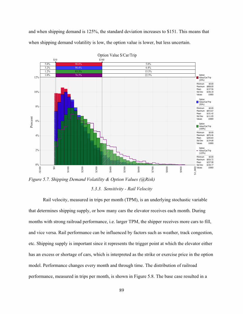
89
and when shipping demand is 125%, the standard deviation increases to $151. This means that
when shipping demand volatility is low, the option value is lower, but less uncertain.
Figure 5.7. Shipping Demand Volatility & Option Values (@Risk)
5.3.3. Sensitivity - Rail Velocity
Rail velocity, measured in trips per month (TPM), is an underlying stochastic variable
that determines shipping supply, or how many cars the elevator receives each month. During
months with strong railroad performance, i.e. larger TPM, the shipper receives more cars to fill,
and vice versa. Rail performance can be influenced by factors such as weather, track congestion,
etc. Shipping supply is important since it represents the trigger point at which the elevator either
has an excess or shortage of cars, which is interpreted as the strike or exercise price in the option
model. Performance changes every month and through time. The distribution of railroad
performance, measured in trips per month, is shown in Figure 5.8. The base case resulted in a

90
mean velocity of 2.58 over all months. For the sensitivity analysis, velocity is held constant at
2.0 TPM and increases to 3.5. Resulting option values are presented in Table 5.4.
Table 5.4. Sensitivity - Rail Velocity
Month/ Velocity 2 2.5 2.58 (Base) 3 3.5 September $117 $198 $246 $308 $438 October $102 $158 $164 $223 $297 November $91 $136 $143 $197 $273 December $81 $125 $134 $180 $245 January $63 $100 $106 $150 $219 February $68 $110 $108 $164 $229 March $103 $156 $159 $219 $298 April $135 $195 $203 $266 $345 May $191 $263 $297 $341 $430 June $181 $250 $261 $328 $410 July $165 $230 $215 $301 $380 August $123 $181 $184 $244 $311 Average $118 $175 $185 $243 $323
Figure 5.8. Velocity Distribution - All Months (@Risk)

91
Results show that velocity has a positive impact on option values. With the low-end
velocity of 2.0, the option value is $118, and increases to $323 as performance increases. This
result is expected, since higher velocity, and therefore higher shipping supply, means that there is
a better chance that the elevator would have excess cars that can be sold into the secondary
market. The relationship between velocity and option value is non-linear, and is slightly
exponential, as shown in Figure 5.9 with the spread between simulation results increasing from
$57 to $80. This is an important result as it shows the significance of projecting railcar velocity
when making car-ordering decisions. Shippers who expect strong performance would not need to
buy as many shuttle contracts as one who predicts weaker performance. However, they may
consider keeping up order quantities since there is greater option value under this circumstance.
Figure 5.9. Option Values and Velocity

92
5.3.4. Sensitivity – Futures Price Spreads
Futures price spreads refer to the inter-month price differences in each contract month.
When deferred contract months are at a premium to nearby months, it is referred to as a “normal”
or positive spread market. When the opposite is true, the market is referred to as “inverted.” The
same principle applies to basis values, but here we focus on futures. During times with large,
positive spreads, the shipper is encouraged to store their grain since they can hedge at a higher
price in the deferred months. Inverted markets encourage shipment of grain, since the elevator
would be losing money by storing into a contract month with lower prices. Soybeans is a market
in particular that exhibits both normal and inverted price spreads at different times. Therefore, it
is beneficial to examine how these spreads impact shipping demand, and overall option values.
The base case spreads are presented in the table of the previous chapter. For the sensitivity
analysis, the inter-month spreads begin at -$0.15, and increase to $0.15.
Results are presented in Table 5.5 and demonstrate a positive relationship between price
spreads and option values. In a strongly inverted market, the transfer option is worth $152, and
increases to $293 as the market becomes normal with positive spreads. This is largely explained
by the impact on ship vs. storage decisions, which is reflected in shipping demand. As shown in
Figure 5.10, where shipping demand in cars is on the horizontal axis, the distribution of shipping
demand shifts to the left as the futures price spreads increase. In the simulation with negative 15
cent spreads, the elevator is encouraged to ship grain immediately rather than store, and the
average monthly shipping demand is 670 cars per month. The simulation with positive 15 cent
spreads results in average shipping demand is lower at 593 cars per month. As previously
demonstrated, shipping demand and option values have a negative relationship with each other.

93
Table 5.5. Sensitivity - Futures Price Spreads
Month/Futures Spread -$0.15 -$0.05 Base $0 $0.05 $0.15 September $238 $331 $246 $413 $528 $921 October $124 $136 $164 $148 $164 $214 November $53 $98 $143 $127 $163 $246 December $129 $132 $134 $136 $144 $168 January $55 $82 $106 $100 $122 $159 February $109 $110 $108 $113 $116 $131 March $78 $121 $159 $147 $176 $228 April $206 $206 $203 $209 $213 $228 May $172 $234 $297 $282 $340 $415 June $282 $278 $261 $275 $276 $254 July $162 $215 $215 $247 $276 $285 August $213 $231 $184 $244 $256 $262 Average $152 $181 $185 $203 $231 $293
Figure 5.10. Sensitivity - Futures Price Spreads and Shipping Demand (@Risk)

94
5.3.5. Sensitivity – 2013/2014 Scenario
Late 2013 into 2014 presented a unique situation and many challenges for grain shippers
in the upper Midwest. The main factors were a large 2013 harvest and competition for track
space brought on from peak oil production in western North Dakota. An inverse in futures prices
also encouraged elevators to ship grain at a more rapid pace. This unprecedented track
congestion caused low railcar velocity, and extremely high secondary market prices, peaking
around $5,000.
Recreating this scenario in the model provides insights into the value of transferability
during shocks to the shipping system. While it is impossible to reconstruct every aspect of the
2013/2014 shipping season, four key variables are highlighted: decreased velocity, increased
farmer sales, an inverse in futures prices, and large secondary market prices. This is simulated by
setting velocity at 2.0 trips per month, secondary market prices at $2,500, and the futures price
spreads to -$0.05 from each contract month to the next. Also, the large crop is simulated by
increasing the elevator turnover ratio, U, from six to eight, which increases the annual amount of
grain handled, ℎS, from 30,000,000 bushels to 40,000,000. Since the situation was unpredictable
for the most part, we assume the elevator keeps the same car order strategy and purchases two
shuttle contracts in the primary market. Resulting option values, shipping demand, and volatility
are presented in Table 5.6.

95
Table 5.6. Sensitivity - 2013/2014 Scenario
Option Value Ship Demand
(Cars) Ship Demand
Vol. September $407.45 559 40% October $57.11 853 47% November $44.22 870 47% December $45.15 871 42% January $42.49 878 38% February $39.65 876 35% March $45.97 875 33% April $59.76 863 32% May $84.44 846 31% June $142.81 817 32% July $162.78 807 34% August $251.00 750 38% Average $115.24 822 39%
Results show that the transfer option value decreases to $115. This is mainly due to the
increased shipping demand from the large crop, and decreased volatility. Also, the decreased
velocity means that there are fewer excess car situations, and therefore fewer railcars available
for resale into the secondary market. In reality, times of such high secondary market prices may
cause the shipper to forgo grain sales and instead sell railcars, which is not accounted for in this
model since the primary objective for the elevator is to sell grain. A shipper who is willing to
forgo grain sales in this situation would place a much higher value on the transferability. Either
way, a shipper who had shuttle contracts during this period had more flexibility than one who
relied on secondary market cars, or other instruments.
5.4. Strategic Sensitivity – Railcar Ordering Strategy
This section presents a sensitivity analysis on a key strategic variable, railcar ordering
strategy. Strategic variables refer to those that are decided upon by the elevator manager. The
base case assumes a typical strategy for each variable based on discussions with the industry

96
sources previously mentioned. However, each elevator makes different decisions, so it is
important to analyze the impact of each possibility on the transfer option.
The analysis is set up the same way as the stochastic sensitivity. One at time, multiple
simulations are run for possible inputs for each decision. The seed generator is set so that each
simulation produces the same stochastic input values. Results and implications for each variable
are discussed.
Railcar ordering strategy refers to the amount of shuttle contracts the elevator purchases
at the beginning of the marketing year. The base case assumes that the shipper orders enough
shuttles to fill as close to 100% of the annual projected shipping demand as possible. Assuming
the shipper expects the rail carrier to average 2.5 trips per month, they would purchase two
shuttle contracts. For whatever reason, a shipper may decide to purchase enough cars to cover
more or less than the projected shipping demand. For the sensitivity analysis, the strategy starts
at 60% and increases to 140% of projected shipping demand. Results are presented in the table
below.
Results in Table 5.7 show a positive relationship between the number of shuttle contracts
and option values. This is explained by the fact that more shuttle contracts provide greater
shipping supply. Higher shipping supply then increases the possibility of having excess cars to
sell into the secondary market. This has large implications for a one-location grain shipper, since
any change in car ordering strategy can cut their shipping supply in half, or double it.
Alternatively, if a larger shipper added one or two shuttles to their fleet, the marginal percentage
change in shipping supply would be smaller. These sensitivity results show the impact of an
elevator’s car ordering strategy on the value of transferability.

97
Table 5.7. Sensitivity - Railcar Ordering Strategy
Month/ Order Strategy
60% (1 Shuttle)
100% (Base, 2 Shuttles)
140% (3 Shuttles)
September $119 $246 $400 October $86 $164 $236 November $86 $143 $225 December $79 $134 $205 January $51 $106 $183 February $55 $108 $173 March $92 $159 $232 April $136 $203 $266 May $227 $297 $359 June $198 $261 $314 July $155 $215 $260 August $111 $184 $234 Average $116 $185 $257
5.5. Summary
In order to evaluate various shipping instruments available to grain elevators, valuing
individual components within each instrument helps to determine the overall value of the
contract. One of the common components seen in today’s shuttle contracts is the ability to
transfer excess cars into a secondary market and receive the resale price. Due to the qualitative
and contingent nature of this component, real option analysis is an appropriate valuation
technique. An empirical model was defined, along with base case inputs and key parameters.
This chapter presented the results from the base case, and the results of a sensitivity analysis on
key stochastic and strategic inputs.
The base case results indicate that this transfer option is worth $185 per car, per trip,
meaning that the shipper should pay this much of a premium for a contract that allows
transferability versus one that does not. On a monthly basis, this transfer option is worth the most
in May at $297, and the least in January at $106. Shipping demand was found to have a negative

98
relationship with the option value. During months with high shipping demand, such as harvest,
the option is worth less due to fewer prospective cars being available for resale, and vice versa.
A sensitivity analysis was conducted on key inputs to demonstrate the impact of the
variable on the option value. The stochastic variables included in the sensitivity section are
secondary market prices, shipping demand volatility, velocity, and inter-month futures price
spreads. Secondary market prices are shown to have a strong, positive relationship with option
values, which is expected. Shipping demand volatility also has a positive relationship with option
values, which corroborates with option pricing theory. Also causing increases in option values
are increases in rail velocity, due to the fact that it increases shipping demand, meaning that more
excess cars are available for sale. Futures price spreads are shown to have a negative impact on
shipping demand, which results in a positive impact on option values. This is due to the fact that
larger price spreads encourage shippers to store more grain, and vice versa. Results from the
2013/2014 scenario simulation indicated the option value drops to $115 during times of large
crops, and increased track congestion.
The impact of the shipper’s railcar ordering strategy is also analyzed. Railcar ordering
strategy is shown to have a positive impact on option values. This occurs since buying more
shuttles increases shipping supply, and therefore the number of excess cars available to transfer.
From these results, one may infer that it is best to order as many shuttles as possible regardless of
shipping needs. However, there is risk in that if secondary market prices collapse, the elevator
could be stuck with lots of extra freight that they either cannot find a buyer for, or must sell at
negative values.

99
6 CHAPTER 6. CONCLUSION
6.1. Introduction
Grain shippers face many sources of risk and uncertainty in their operations, and these
risks are unique to each shipper. Country elevators are essentially the middleman between
farmers and end users of grain. They make money by purchasing grain from farmers, selling to
the next user, and arranging shipping and handling. Margins for a country elevator are usually
quite thin. Therefore, they rely on shipping large volumes to make a profit. In most cases, it is up
to the elevator to plan and pay for shipping from their location to the buyer. With narrow profit
margins, proper planning of logistic needs can be the difference between positive and negative
returns.
In the upper Midwest, logistics planning is more crucial since modes of transportation are
limited. Without direct access to a river large enough for barges, shippers must utilize either
trucks or railways. Trucks are okay for short hauls, but due to economies of scale, rail is the only
viable choice to get grain to the port from inland locations. With soybean acreage on the rise, and
the Pacific Northwest (PNW) being the main destination for North Dakota-grown soybeans,
producers and shippers will only become more reliant on rail transportation.
In order to plan for logistics, shippers have to not only plan out the quantity of shipping
needs, but also value the cost of obtaining railcars. Since each rail carrier offers different contract
instruments, and each elevator has different needs, placing a value on rail transportation can be
quite abstruse. Due to both spatial and temporal differences in shipping needs among different
elevators, rail carriers have been offering various forms of flexibility within their contracts,
which add value to the instrument. One of the main flexible components offered by carriers, such
as BNSF, is the ability to sell or transfer unneeded cars into a secondary market. This adds value

100
since it gives the shipper the chance to recover some of the sunk costs of purchasing rail service.
Without this transferability, the shipper would be forced to either use the cars, cancel them for a
penalty, or let them sit idle and pay significant demurrage charges. Also, they may under-order
the amount of cars they need, since any excess cars would present a larger cost.
The primary goal of this study is to value this transferability using real option analysis.
Determining the relationships between key variables and the transfer value are examined as
ancillary objectives. Previous chapters presented the risks inherent for a grain shipper, current
railroad contracting mechanisms, an overview of real option pricing, and an empirical model for
valuing this transferability as a European put option. Results of the empirical model were then
presented for the base case and various sensitivities. This chapter reviews these concepts,
including the problem statement, railroad contracting mechanisms, real options, the empirical
model, and results, following by the implications for shippers and carriers. A summary then
includes the contribution to literature, limitations of the study, and suggestions for further
research.
6.2. Problem Statement
Elevators face various forms of risk due to the risky dynamic variables in grain trading.
One major source of risk for an elevator is their inventory levels. A majority of country elevator
grain purchases come in the form of “spot” deliveries. This occurs when farmers choose to haul
in grain and receive the price that the elevator has posted for the day. Since the farmer has
control of the decision to initiate a spot delivery, the elevator is uncertain about how much grain
they would have on hand at any point in the future The elevator can entice spot deliveries by
increasing their bid price, but must then sacrifice some profitability. One way to guarantee grain
inventory in the future is to offer various forms of forward contracts. This is useful for planning

101
out inventory levels, but again must offer a price that is attractive to producers. Variable
inventory levels make it difficult for elevators to project what their demand for railcars, or
shipping demand, would be in the future.
Another major source of risk for a grain shipper is the price they must pay for railcars.
This is true for shippers who do not utilize primary market shuttle contracts, and rely on
secondary market purchases. Just as grain prices fluctuate daily, so do transportation costs.
Although the price the elevator pays depends on the rail carrier and pricing mechanism, there are
essentially two costs of railcar shipping: the tariff rate and the price to secure cars (if buying in
the secondary market). The tariff rate is what the shipper pays for each move from origin to
destination. Every origin/destination combination has a unique tariff rate that is subject to change
each month. The cost of securing cars depends on the contract mechanism, and supply and
demand factors within the rail market. A shipper who does not forward contract shipping needs
is subject to a different price every time they purchase railcar trips. The cost just to secure cars
can be anywhere from -$400 to $5,000 over tariff per car. This means the shipper may have to
pay over a dollar per bushel just to secure transportation. There are also times when this cost of
securing cars is negative, which means that the shipper could be paid just to utilize someone
else’s unneeded cars. Therefore, the cost of shipping would be less than the tariff rate. The
average secondary market price since 2004 is $213/car, versus only $50-$100 in the primary
market. Also, a secondary market buyer faces greater price volatility.
To mitigate risk from grain price movements, there are established futures and options
markets, as well as forward contracting mechanisms. However, there is no such derivative
market for railcars. Therefore, the only way for an elevator to lock in a shipping rate is through
some type of forward contract.

102
Although forward contracting rail service from a carrier provides a locked-in price, the
shipper is still exposed to railroad performance risk. Performance risk affects the number of
trains that the shipper receives each month. Performance is known as train velocity, and is
measured in trips per month. Each time the train completes a cycle from origin, to destination,
and back to an origin, is considered one trip. Although an experienced elevator manager would
have some idea of the amount of cars they need to utilize, the specific amount is at the mercy of
the shipping conditions. These conditions include weather, track congestion, etc. If bad weather
occurs, such as an avalanche blocking off track, trains would be backed up. Track congestion
from other commodities, such as oil, can also cause bottlenecks and service delays. Therefore,
the amount of cars received each month, or shipping supply, is a random or stochastic variable.
Combined with inventory level risk, this means that both demand for railcars, and supply of
railcars is uncertain for a shipper.
6.3. Current Railroad Pricing/Contracting Mechanisms
Chapter 2 describes the railcar contracting mechanisms currently available to grain
shippers. As there are a number of different rail carriers, and each carrier offers their own
programs, there are many different railcar pricing and contracting mechanisms. However, since
rail carriers own most of the track space, shippers are subject to utilize whoever owns the track
on which they are positioned on. In order to meet changing needs of grain shippers, carriers
change their car programs throughout time. This study focuses on the current shipping programs
offered by BNSF, and specifically their shuttle program. A shuttle refers to a 110-car train unit,
which is designed to be kept in constant use. It is intended for elevators that ship large volumes
of grain throughout the year. See Table 2.1 in Chapter 2 for details on the BNSF shuttle program.

103
There are essentially two ways for a shipper to secure shuttles through BNSF: through the
primary market, or the secondary market. The primary market is the initial allocation of railcars
from the carrier to the shipper. Through an auction system, the winning shipper receives the
rights to a shuttle contract lease for one year. The shuttle is meant to be kept in constant use by
offering financial incentives for quick loading at the elevator. If the train is not loaded within 24
hours, the shipper must pay a demurrage penalty each hour until the train is released. The
primary owner only pays the tariff rate each time they utilize the cars, but are still subject to
railroad performance risk. The owner has the ability to switch origins, free of charge, as long as
they notify BNSF before it reaches the prior destination. A major component of these contracts,
and the focus of this study, is the ability to not only switch origins, but transfer the service to
another shipper, which is the basis for the secondary market.
The secondary market refers to transactions between two different shippers. The primary
owner of a shuttle contract can sell any unneeded trips to another shipper at a market-based
price. This can be negotiated privately between shippers, or done through a third-party broker.
During times of high demand for railcars and low railcar availability, prices in the secondary
market would be a large premium to the tariff rate. If the opposite is true, the primary owner may
have to pay another shipper to utilize the cars in the secondary market. In times of negative
secondary market prices, the shipper must weigh their options of selling the cars at a loss, finding
a way to utilize them, or pay a steep cancellation fee. Under cancellation, the owner forfeits all of
the remaining trips of the contract.
This transferability is key as it allows the primary shuttle owner to receive revenue for
any unneeded cars, and eliminate their obligation. There are also times when secondary market
prices become high enough that it is more profitable to sell railcars in lieu of shipping grain.

104
6.4. Real Option Pricing Methodology
Chapter 3 describes real option analysis, including its uses and solution methods.
Traditional valuation methods, such as net present value, provide basic formulations for
analyzing the quantitative aspects of capital expenditures. However, there are many qualitative
aspects of some investments that require deeper analysis in order to estimate the true value.
Many investments provide various forms of flexibility, either implicit or explicit, that provide
value to the project. For example, making an expenditure now may allow the investor the option
to make a further investment in the future, depending on the success of the first project. The
value of the initial investment may be dependent on the value of the future investment, and must
be considered in the initial cash outlay.
Real option analysis (ROA) has developed as a way to value contingent investment
decisions. The more flexibility and uncertainty inherent in a project, the more useful ROA is as
valuation tool (Trigeorgis 1996). Using option pricing theory and applying it to real assets, ROA
allows for valuation of future decisions that are contingent on prior events.
There are many different types of optionality apparent in capital expenditures. For
example, there are options to delay, expand, or abandon an investment. Anyone who has
purchased car insurance has purchased a real option, since the owner has the option to sell their
car for the full amount after an accident, even if the car’s price drops to the scrap value. The
insurance payment is contingent on whether an accident occurs or not. Similar to financial
options, the more volatile the underlying variable is, the more the option is worth. A car owner
with a history of bad driving causes the car’s value to become more volatile, which is why they
pay a higher premium than someone with a clean driving record.

105
An option to sell, also called an abandonment or transfer option, allows the owner to get
out of an investment in the future if they find it is not profitable, and recover some of the initial
cost. This option adds value to the initial investment, since it decreases the amount of risk that
the manger is taking on. One of most common ways to calculate the value of a transfer option is
with a binomial option pricing model, either stochastic or static.
6.5. Empirical Model
Chapter 4 presents the empirical model for valuing the transferability of primary shuttle
contracts as a real option. In financial options, if the underlying futures price drops below the
strike price, the owner of a put option can exercise their right to sell at the strike price. The same
principle applies to transfer options. If the value of a project drops below a certain level, the
owner of the option can sell the underlying asset. This can then be modeled as a put option
(Winston 2008, Alizadeh and Nomikos 2009).
Since the owner of a primary shuttle contract has the right, but not the obligation to sell,
or transfer railcars into the secondary market, this flexibility provides value since the owner is
not required to use their entire supply of railcars. Assuming that the objective for an elevator is to
sell grain first, and excess railcars second, the underlying variable for the option is demand for
railcars, or shipping demand. If shipping demand is lower than shipping supply, the owner now
has excess cars to sell into the secondary market. This concept provides the basis for valuing the
transferability of railcars as a real option. The owner is assumed to make the decision regarding
excess railcars at the last possible moment. Therefore, this is synonymous to a European put
option.
The empirical model consists of two main parts: a material requirement planning (MRP)
schedule, and the stochastic binomial option pricing trees. Module 1, the MRP schedule,

106
represents the grain inflows and outflows for a typical country elevator. The purpose is to derive
projections for shipping demand, and shipping demand volatility, which are used in the pricing
trees. The first part of the MRP schedule projects farmer deliveries for each month. This is based
on the elevator storage capacity, an inventory turnover ratio, and data on farmer sales during
each month of the marketing year. Futures prices, basis levels at the Pacific Northwest, and
storage costs then determine the optimal months to sell grain in. Once this is compiled, an initial
shipping demand schedule is estimated. Before the final level of monthly shipping demand is
derived, adjustments are made for storage and shipping capacities. Everything is also rounded to
units of 110 cars, since shippers must utilize the entire train capacity. Once shipping demand is
projected, shipping demand volatility is derived.
Module 2 consists of 12 different stochastic binomial option pricing trees, one for each
month. Shipping demand, volatility, time until expiration, and the risk-free rate are used to
calculate “up” and “down” factors for each option tree node, as well as the risk-neutral
probability. Each month also has a unique strike value, which is the amount of railcars supplied.
The binomial lattices are constructed with the first branch of each month being the projected
shipping demand from the MRP schedule, measured in railcars. The end nodes represent possible
shipping demand levels for each month. The range of shipping demand levels depends on the
volatility, and the amount of branches is determined by the option month.
Based on the level of shipping demand at each end node and the strike value, which is the
amount of cars supplied, there is either an excess or shortage of cars. In cases of a car shortage,
the shipper would buy in cars, and the transferability would have no value. When there is an
excess amount of railcars, the shipper then has three alternatives: sell the cars, utilize them, or
cancel the contract. Payoffs for all three choices are defined, and the shipper chooses the

107
alternative with the highest value. When selling cars provides the highest payoff, the
transferability has value. The value is defined as the marginal difference between selling cars,
and the next best alternative. Once values are calculated at each end node, they are discounted
back to the present based on the interest rate, and risk-neutral probability.
Once monthly transfer option values are derived, they are converted into per-car, per trip
units. The average of all 12 monthly values is used to describe the overall transfer option value.
Sensitivities are then conducted on run on key stochastic and strategic inputs to gauge their effect
on the option value.
Monthly data for basis levels, farmer sales, and secondary rail prices extends from 2004
through 2016, and railcar velocity data runs from 2011 through 2016. Farmer sales and velocity
exhibit strong seasonality, and basis levels have an upward trend. This data and resulting
distributions are presented in the tables in Chapter 4.
6.6. Results
The model represents a North Dakota soybean shipper who sells to export terminals in
the PNW using primary shuttle contracts that run from September through the following August.
Monte Carlo simulations are implemented using @Risk to simulate 10,000 iterations of the MRP
schedule and stochastic binomial option pricing trees. The four stochastic variables were PNW
basis values, farmer sales, secondary rail market prices, and railroad velocity. Transfer option
values are calculated for each month, and the average of all monthly values represents the overall
transfer value. Simulation results for shipping demand, shipping demand volatility, secondary
market prices, and velocity are also presented. A sensitivity analysis was then conducted on key
input variables.

108
6.6.1. Conclusions from Base Case
The base case assumes the elevator has 5,000,000 bushels in capacity, and that they turn
their inventory over about six times each year. They forward contract 25% of their grain receipts,
and can ship a maximum of eight trainloads each month. Also, they order enough shuttle
contracts to cover close to 100% of their projected shipping demand.
The average value of the transfer option value is $185, meaning that of the total contract
price, $185 is derived from the ability to sell excess cars into the secondary market. However,
this value varies substantially, as shown in Figure 6.1. The large variance is mainly attributable
to large volatility in both secondary market prices, and shipping demand. The lowest possible
value is $0, and the highest value out of 10,000 iterations is $947. High values occur during
periods of high secondary market prices, low shipping demand levels, high shipping demand
volatility, and low velocity, which decreases shipping supply. The 90% confidence interval for
the overall value is $14-$461. Also, distribution of outcomes is highly skewed to the right, as
shown in Figure 6.1.
The largest monthly value is in May at $297, and the least occurs January at $106. This
coincides with low shipping demand in May, and high shipping demand in January. In months
with low shipping demand, the elevator has more excess cars to sell, which increases the transfer
option value, and vice versa. The high shipping demand in January can be explained by large
inventories of grain from the recent harvest. Low shipping demand occurs in the summer into
early fall, since farmer sales are mostly completed by then. Secondary rail market prices and
shipping demand volatility are shown to have fairly strong positive correlations with the average
option values with coefficients of 0.63, and 0.49, respectively.

109
6.6.2. Conclusions from Sensitivity Analysis
In order to estimate the impact of key input variables on the transfer option value,
sensitivity was conducted on secondary market prices, shipping demand volatility, rail velocity,
futures price spreads, railcar ordering strategy, and forward grain contracting strategy. The
scenario in the 2013/2014 crop year was also recreated to demonstrate how shocks to the rail
system impact the transfer option.
Secondary market values demonstrate a positive relationship with the option value, since
it directly impacts the revenue the shipper receives for selling excess cars. Shipping demand
volatility also has a positive relationship with the transfer option value, which aligns with option
pricing theory. Velocity and car ordering strategy both have a positive relationship with the
option value, since these variables determine the supply of railcars. The car ordering strategy
refers to the percent of projected shipping demand that the elevator forward contracts in the
Figure 6.1. Base Case Distribution of Option Values (@Risk)

110
primary market. When supply is increased, there is a better chance that the shipper has excess
cars to sell into the secondary market. However, this does not necessarily imply that the shipper
should order as many contracts as possible, since they are at risk of the secondary market prices
collapsing, and/or not being able to find a buyer in the secondary market. Futures price spreads
have a positive impact on the option value, since large price spreads encourage the elevator to
store rather than ship grain, which lowers shipping demand. The 2013/2014 simulation indicates
that periods of large crops and high track congestion cause the option value to decrease, but this
relationship depends on the shipper’s strategy. These results are summarized in Table 6.1.
Table 6.1. Summary of Results
Variable Relationship with Transfer Option Value
Base Case $185 (Average)
Secondary Rail Market Prices Positive
Shipping Demand Volatility Positive
Railcar Velocity Positive
Futures Price Spreads Positive
Railcar Ordering Strategy Positive
6.7. Implications of Results
This section highlights the implications of the results from the base case and sensitivity.
Implications are important since they link the results to application. Results of the transfer option
model have implications for both shippers and carriers.
6.7.1. Implications for Shippers
This option value helps shippers gain insight into the value of various components of the
overall contract price. For the transfer option to have value, or to say that it is “in the money,”
two things need to happen: the shipper must have excess railcars, and selling these excess

111
railcars must be the best alternative compared to utilizing them, or cancelling the contract.
Whether or not the shipper has excess cars depends on the relationship between the underlying
variable, and the strike value, which in this case are shipping demand, and shipping supply,
respectively.
While the overall price of the shuttle contract is determined by the auction process, the
transfer option is an implied value to the shipper. Another way to interpret this value is the
premium, or marginal difference in a hypothetical contract that offers transferability versus one
that does not, ceteris paribus. The value implies that whenever the primary shuttle contract cost
is less than the transfer option value, there is extra value for the shipper since the transferability
alone is worth, on average, $185. If the contract costs more than the transfer option value, any
extra value to be gained by the shipper depends on competing auction bids, and the shipper’s
forecasts regarding future transportation needs and prices. Since shuttle contracts typically cost
between $50 and $150, and the average transfer option value is $185, this flexibility does
provide substantial value to the shipper. Also, this raises the possibility that shippers under-value
the transferability embedded within these shuttle contracts, or do not fully acknowledge it.
This result only applies to the base case situation. The sensitivity provides insights to
how this value changes with different input values. An advantage of this model is the ability to
calculate the option value for any range of expectations regarding input variables.
The overall implication for shippers is that contracts with transferability do provide
additional value. It allows the shipper to match levels of shipping supply with their shipping
needs, and also provides an additional source of revenue. Without the option to transfer excess
cars, the shipper would be inclined to forward contract fewer cars, since both cancelling the

112
contract and forcing a grain shipment can be costly. Forward contracting fewer cars then exposes
the shipper to more price risk.
6.7.2. Implications for Carriers
These results also have implications for rail carriers. Since the option value alone is
worth more than what the contracts usually sell for, it shows that the carriers are doing a good
job of designing the instruments so that they provide value for their customers. This implies that
the carrier could capture more profitability while still providing additional value to the shipper.
However, this is more difficult to value as a carrier, and with an auction-based allocation system,
the carrier is not in complete control of the selling price for shuttle contracts. Mainly, it shows
that the transferability they offer does provide value for their customers.
An indirect impact of the option is that offering this transferability helps support basis
levels for farmers. When shippers are more efficient with transportation needs, they are able to
move more inventory, and therefore offer competitive bids to farmers for their grain. However,
this idea would need to be studied further.
6.8. Summary
Grain shipping involves many dynamic variables, and in response to the changing needs
of elevators, railroad carriers offer various forms of flexibility within their contracts. One of the
main components of these contracts allows the shipper to transfer any excess or unneeded
railcars into a secondary market. The primary objective of this analysis has been to value this
transfer option as a European put using real option analysis. Results indicate the option is worth
$185 per car, per trip, but depends heavily on assumptions about key stochastic and strategic
variables that may best be determined by the shipper utilizing the shuttle contract. This section

113
highlights the contribution to literature, limitations of the study, and provides suggestions for
further research.
6.8.1. Contribution to Literature
This thesis extends the literature on grain transportation by rail, and real option analysis.
Most studies on grain shipping aim to analyze relationships between certain variables, but little
has been done in regards to contract pricing, and no research has valued the transferability
inherent in current shuttle contracts. This study also provides sensitivity results which describe
the impact that key inputs have on the option value.
With the exception of Lee (1999), real option analysis has not been applied railroad
shipping instruments for a grain company. Whereas most real option studies use the dollar value
of the project as the underlying variable, this application is unique in that it utilizes demand for
railcars as the basis for the contingency decision. This is aimed to better reflect the decisions that
grain shippers make in regards to railcar sales. This study builds on the work of Lee (1999) by
adding a material requirement planning schedule to project shipping needs, and modified option
payoff functions to reflect all of the choices available to a shipper under excess-car situations.
There have been numerous changes in the shuttle contracting instruments within the last 20
years, which are reflected in the model along with more complete datasets of stochastic
variables. This model also includes time series analysis, which is only available in @Risk
versions after 2012. This allows stochastic forecasts to better account for seasonality and trend.
6.8.2. Limitations
This study is limiting in that it does not value the entire shuttle contract value, but rather
just one component of it. Valuing the whole shuttle contract would require more complex
analysis, including bidding strategy. Also, it is difficult to quantify the value of railcars that are

114
used to ship grain, since they are then considered an input for the business rather than a source of
revenue.
Since some of the base case assumptions and parameters greatly impact the option value,
this model is better suited to provide a guide to valuing the transferability, rather than a definitive
result. Therefore, logistics managers must consider inputs that are unique to their business when
valuing shipping mechanisms.
The base case result of $185 must be considered cautiously, since it is higher than the
normal range of the total shuttle contract cost of $50-$150. Part of this is high result is from the
fact that secondary rail market prices rose steeply in the fall of 2016. Since the stochastic
projections are based off of the last historical data point, this caused the projected prices to
average $411, whereas the entire historical dataset only averages $213. Also, high volatility of
shipping demand contributes to the large option value. This is from the “all or nothing” aspect of
the MRP schedule. When it is economical to sell grain, the elevator ships the whole inventory,
up to the shipping constraint. In reality, shippers have the ability to lower this volatility by
strategically evening out the level of shipments each month.
Other limitations include the assumptions about being a soybean-only shipper, and only
having one market to sell to. In actuality, nearly all country elevators handle multiple
commodities and sell to multiple destinations. However, the assumption about having only one
sale market is light since 72% of North Dakota-grown soybeans are sold to the PNW (North
Dakota Soybean Council). The model also assumes elevator inventories only consist of spot
deliveries and forward contracts. Many elevators also offer other forms of grain contracting
strategies such as hedge-to-arrive, storage, and average-price contracts.

115
Lastly, we assume that there is enough liquidity in the secondary market to find a buyer
for every excess railcar that the shipper wishes to sell. In reality, there may be times when there
is no one to sell the excess cars to. This impact would lower the transfer option value.
6.8.3. Further Research
Using the framework and concepts from this study, there are many possibilities for future
studies. One may be to explore other options embedded within shuttle contracts. While
transferability is the main component, the ability to cancel the contract could be modeled as an
abandonment option. This requires projections about the future secondary prices at each point in
time. Essentially, a different forward curve of prices would need to be projected each month. The
transfer option could hypothetically be modeled as an American option, but would require more
complex analysis regarding shipping demand projections, and the consideration of early exercise
at each node. An American option approach would imply that the shipper can forward sell cars
months ahead of time. This study focuses on sellers of secondary railcars, but the same
framework can also be applied to a buyer of secondary cars, in which case the transferability
would be modeled as a call option. The call option would have value when the shipper is short,
or in need of railcars.
The transferability component of shuttle contracts can be studied in many different
realms. Quantifying the impact that transferability has on elevator basis levels would provide
insights on the overall benefit that these contracts provide. One issue in grain shipping is the
seasonality of grain flows, and future studies could examine if offering transferability in shuttle
contracts has an effect on this seasonality. While this study shows that transferability has value
for the shipper, a cost/benefit analysis for the carrier could be conducted as well. Also, this

116
model could be used in addition to other methods in valuing the entire primary market shuttle
contract for a shipper. An extension would be to model secondary rail market values.
This framework provides the possibility of further research on option valuation for
shippers involving multiple locations, commodities, and sale markets. The model could be
modified to reflect a shipper who is willing to forgo grain sales if it is more profitable to sell
railcars instead. This would change the model structure so that the underlying contingency
variable is the secondary market price, rather than shipping demand levels.

117
7 REFERENCES Alizadeh, Amir H., and Nomikos, Nikos, K. 2009. Shipping Derivatives and Risk Management. New York: Palgrave Macmillan. Amram, Martha., and Kulatilaka, Nalin. 1999. Real Options: Managing Strategic Investment in an Uncertain World. Boston: Harvard Business School Press. Babcock, Michael W., and Gayle, Philip G. 2014. “Specifying and Estimating a Regional Agricultural Railroad Demand Model.” Journal of the Transportation Research Forum 53(1):35-48. Babcock, Michael W., McKamey, Matthew, and Gayle, Philip. 2014. “State Variation in Railroad Wheat Rates.” Journal of the Transportation Research Forum 53(3):83-100. Bernard, Jean-Thomas., Khalaf, Lynda., Kichian, Maral., and McMahon, Sebastien. 2015. “The Convenience Yield and the Informational Content of the Oil Futures Price.” Energy Journal 36(2):39-46. Burlington Northern Santa Fe. 2016. Jumbo Covered Hopper Car Dimensions. Web. ———. 2016. Railroad performance data from January of 2011 to September of 2016. Web. ———. 2014. “STB Ex Parte No. 724 (Sub-No. 2), United States Rail Service Issues-Grain.” Filing to the Surface Transportation Board. Choi, Tsan-Ming., Chiu, Chun-Chun Hung., and Chan, Hing-Kai. 2016. “Risk Management of Logistics System.” Transportation Research Part E 90:1-6. Churchill, Jason. 2016. “Valuation of Licensing Agreements in Agriculture Biotechnology.” MS thesis, North Dakota State University. Cox, John C., Ross, Stephen A., and Rubinstein, Mark. 1979. “Option Pricing: A Simplified Approach.” Journal of Financial Economics 7(3): 229-263. Dahl, Bruce L., Wilson, William W., and Gustafson, Cole R. 1999. “Option Values for Provisions in Export Credit Guarantees.” Journal of Agricultural and Resource Economics 24(2):506-524. Data Transmission Network (DTN) ProphetX. 2016. Chicago Mercantile Exchange Soybean Futures prices. Retrieved from DTN ProphetX. Dixit, Avinash. 1989. “Entry and Exit Decisions Under Uncertainty.” Journal of Political Economy 97(3):620-638. Dixit, Avinash., and Pindyck, Robert. 1994. Investment Under Uncertainty. Princeton University Press.

118
Flood, Mark D. 1990. On the Use of Option Pricing Models to Analyze Deposit Insurance.” Federal Reserve Bank of St. Louis Review. 72(1):19-34. Hanson, Steven D., Baumel, C. Phillip., and Schnell, Daniel. 1989. “Impact of Railroad Contracts on Grain Bids to Farmers.” American Journal of Agricultural Economics 71(3):638-646. Hanson, Steven D., Baumhover, Stephen B., and Baumel, Phillip C. 1990. “The Impacts of Railroad Transportation Costs on Grain Elevator Handling Margins.” North Central Journal of Agricultural Economics 12(2):255-266. Hyland, Michael F., Mahmassani, Hani S., and Mjahed, Lama Bou. 2016. “Analytical Models of Rail Transportation Service in the Grain Supply Chain: Deconstructing the Operational and Economic Advantages of Shuttle Train Service.” Transportation Research Part E 93:294-315. Ihli, Hanna J., Maart-Noelck, Syster C., and Musshoff, Oliver. 2013. “Does Timing Matter? A Real Options Experiment to Farmers’ Investment and Disinvestment Behaviours.” Australian Journal of Agricultural and Resource Economics 58:430-452. Isik, Murat., and Yang, Wanhong. 2004. “An Analysis of the Effects of Uncertainty and Irreversibility on Farmer Participation in the Conservation Reserve Program.” Journal of Agricultural and Resource Economics 29(2):242-259. Kemna, Angelien G. 1993. “Case Studies on Real Options.” Financial Management 22(3):259- 270. Kub, Elaine. 2015. Insufficient Freight: An Assessment of the U.S. Transportation Infrastructure and Its Effects on the Grain Industry. For the American Farm Bureau Federation. July. Lee, Jonathan. 1999. “Applying Option Theory to Guaranteed Rail Mechanisms.” MS thesis, North Dakota State University. Mark, Darrell R., Brorsen, B. Wade., Anderson, Kim B., and Small, Rebecca M. 2008. “Price Risk Management Alternatives for Farmers in the Absence of Forward Contracts with Grain Merchants.” Choices: A Publication of the American Agricultural Economics Association 2nd Quarter, 23(2):22-25. Martin, Michael V. 1979. “Misallocative Effects of Value-of-Service Rail Grain Rates.” Transportation Journal 18(3):74-83. McDonald, Robert L., and Siegel, Daniel R. 1985. “Investment and the Valuation of Firms when there is an Option to Shut Down.” International Economic Review 26(2):331-349.

119
Miao, Ruiqing., Hennessy, David A., and Feng, Hongli. 2014. “Sodbusting, Crop Insurance, and Sunk Conversion Costs.” Land Economics 90(4):601-622. Miller, John. 2016 "Re: BNSF Agricultural Products Podcast October 14, 2016." Video blog comment to customers. YouTube, 14 Oct. 2016. Web. Myers, Robert J., and Hanson, Steven D. 1996. “Optimal Dynamic Hedging in Unbiased Futures Markets.” American Journal of Agricultural Economics 78(1):13-20. National Farmers Union. 2014. “Johnson Testifies Before STB on Rail Access.” Washington Corner, 2. Web. May. Ndembe, Elvis. 2015. “Hard Red Spring Wheat Marketing: Effects of Increased Shuttle Train Movements on Railroad Pricing in the Northern Plains.” Journal of the Transportation Research Forum 54(2):101-115. North Dakota Soybean Council. 2016. “Developing Markets Worldwide.” Annual Report. Olson, Frayne. 2014. “Effects of 2013/14 Rail Transportation Problems on North Dakota Farm Income.” Executive Summary to Senator Heidi Heitkamp. Onel, Gulcan., and Goodwin, Barry K. 2014. “Real Option Approach to Inter-Sectoral Migration of U.S. Farm Labor.” American Journal of Agricultural Economics 96(4):1198-1219. Pindyck, Robert S. 1988. “Irreversible Investment, Capacity Choice, and the Value of the Firm.” The American Economic Review 78(5):969-985. Prater, Marvin E., Sparger, Adam., Bahizi, Pierre., and O’Neil Jr., Daniel. 2013. “Rail Market Share of Grain and Oilseed Transportation.” Journal of the Transportation Research Forum 52(2):127-150. Rau, Philipp., and Spinler, Stefan. 2016. “Investment into Container Shipping Capacity: A Real Options Approach in Oligopolistic Competition.” Transportation Research Part E: Logistics and Transportation Review 93(2016):130-147. Schmitz, John., and Fuller, Stephen W. 1995. “Effect of Contract Disclosure on Railroad Grain Rates: An Analysis of Corn Belt Corridors.” Logistics and Transportation Review 31(2):97-124. Shakya, Sumadhur., Wilson, William W., and Dahl, Bruce. 2012. “Valuing New Random GM Traits: The Case of Drought Tolerant Wheat.” Dept. Agribusiness & Applied Economics. Report No. 691, North Dakota State University. Siqin, Yu., Bin, Ji, and Jinhai, Chen. 2013. “Container Ship Investment Based on Real Option.” Proceedings of the 2nd International Conference on Systems Engineering and Modeling. Paris, France: Atlantis Press.

120
Sparger, Adam., and Prater, Marvin E. 2013. A Comprehensive Rail Rate Index for Grain. Washington DC: U.S. Department of Agriculture, AMS. April. Thomson Reuters. 2016. PNW Soybean prices from September of 2004 to August of 2016. Retrieved from Thomson Reuters Eikon. Tirupattur, Viswanath., Hauser, Robert J., and Boyle, Phelim P. 1997. American Journal of Agricultural Economics 79(4):1127-1139. Tolliver, Denver., Bitzan, John., and Benson, Doug. 2010. “Railroad Operational Performance in the United States.” Journal of the Transportation Research Forum 49(3):87-100. Tomkins, Claire D., and Weber, Thomas A. 2010. “Option Contracting in the California Water Market.” Journal of Regulatory Economics 37:107-141. TradeWest Brokerage. 2016. “Daily Market Report.” PNW Soybean prices, and Secondary Rail Market values from September of 2004 to August of 2016. December. Trigeorgis, Lenos. 1996. Real Options: Managerial Flexibility and Strategy in Resource Allocation. Cambridge, Massachusetts: The MIT Press. Turvey, Calum G. 2001. “Mycogen as a Case Study in Real Options.” Review of Agricultural Economics 23(1):243-264. Tzouramani, I., Liontakis, A., Sintori, A., and Alexopoulos, G. 2009. “Policy Implementations for Organic Agriculture: A Real Options Approach.” Paper presented at the 83rd Annual Conference for the Agricultural Economics Society, Dublin, 30 March - 1 April. U.S. Department of Agriculture, AMS. 2016. Grain Transportation Report Datasets. Raw data. Washington DC. November. U.S. Department of Agriculture, Office of the Chief Economist and the AMS. 2015. Rail Service Challenges in the Upper Midwest: Implications for Agricultural Sectors – Preliminary Analysis of the 2013-2014 Situation. Washington DC, January. U.S. Depertment of the Treasury. 2016. 10-year Treasury Yield Rates. Web. Usset, Edward. 2014. Minnesota Basis Analysis: Final Report for the Minnesota Department of Agriculture. University of Minnesota: Center for Farm Financial Management. July. Vachal, Kimberly., Bitzan, John., VanWechel, Tamara, and Vinje, Dan. 2011. “Differential Effects of Rail Deregulation on U.S. Grain Producers.” The Journal of Policy Reform 9(2):145-155.

121
Villegas, Laura. 2016. “No Train No Grain: The Impact of Increased Demand for Rail Services by the Energy Sector on Wheat Prices.” Indian Journal of Economics and Development 4(4):1-22. Wilson, William W., Carlson, Donald C.E., and Dahl, Bruce L. 2004. “Logistics and Supply Chain Strategies in Grain Exporting.” Agribusiness 20(4):449-464. Wilson, William W., and Dahl, Bruce L. 1997. “Bidding on Railcars for Grain: A Strategic Analysis.” NDSU Agricultural Economics Report, No. 376. ———. 2011. “Grain Pricing and Transportation: Dynamics and Changes in Markets.” Agribusiness, 27(4):420-434. ———. 2005. “Railcar Auctions for Grain Shipments: A Strategic Analysis.” Journal of Agricultural & Food Industrial Organization 3(2):1-29. Wilson, William W., Priewe, Steven R., and Dahl, Bruce L. 1998. “Forward Shipping Options for Grain by Rail: A Strategic Risk Analysis.” Journal of Agricultural and Resource Economics 23(2):526-544. Winston, Clifford., Maheshri, Vikram., and Dennis, Scott M. 2011. “Long-Run Effects of Mergers: The Case of U.S. Western Railroads.” The Journal of Law & Economics 54(2):275-304. Winston, Wayne. 2008. Financial Models using Simulation and Optimization II. New York: Palisade Corporation. Wynn, Katherine. 2017. “Valuing Genetically Modified Traits in Canola Using Real Options.” PhD dissertation, North Dakota State University.