Real Estate Portfolio Management Paper Master Estate Portfolio Theory... · modern real estate...
22
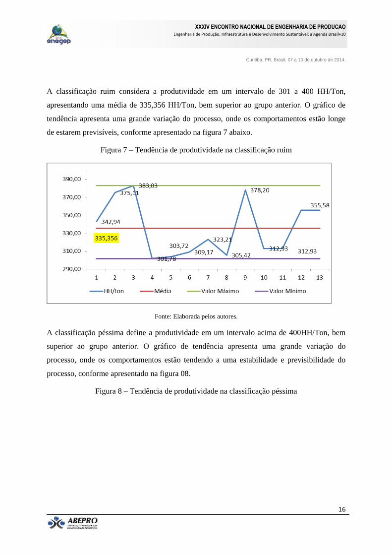
PRODUTIVIDADE NAVAL: UM ESTUDO EMPIRICO DA INDÚSTRIA BRASILEIRA II Maria de Lara Moutta Calado de Oliveira (UFPE ) [email protected] GABRIELA BARROS DE ANDRADE (FMGR ) [email protected] JONATAS DA SILVA JUNIOR (FMGR ) [email protected] Daniela Didier Nunes Moser (UFPE ) [email protected] Elidiane Suane Dias de Melo (UFRPE ) [email protected] Com a retomada recente da indústria naval brasileira foi necessária à quebra da inércia em que o país vivia nesse setor, após cerca de 10 anos praticamente sem desenvolvimento. Os financiamentos do FMM, bem como as demandas crescentes advindas dos programas da TRANSPETRO o PROMEF I e II, além do crescimento do pré-sal, foram essenciais para essa mudança de cenário. Este trabalho tem por objetivo uma análise de índices de produtividade relacionados com a indústria de construção naval nacional. Foram utilizados dados envolvendo os principais estaleiros brasileiros distribuídos em todas as regiões com os diversos tipos de embarcações produzidas ao longo dos últimos seis anos. Como variáveis de análise foram definidos os quantitativos de Hora-Homem de trabalho (HH), peso do aço processado em Toneladas (Ton) e a relação entre essas variáveis, (HH/Ton). Foram comparadas as produtividades de diversos tipos de embarcações com graus de dificuldade de construção diferentes, em estaleiros diversos, com capacidades tecnológicas distintas. Os resultados obtidos foram aplicados na elaboração de uma proposta de sistema de classificação de produtividade para algumas embarcações construídas no Brasil no período de 2006 a 2012, definindo a produtividade de acordo com uma escala Likert como ótima, boa, média, ruim e péssima. Resultados preliminares mostraram que a região Norte, que produz em sua maioria embarcações para navegação interior, tem uma produtividade ótima; enquanto que, nas regiões Nordeste e Sudeste, que produzem embarcações de longo curso e de apoio marítimo e portuário, este índice ainda esta muito longe de ser considerado bom. Isto XXXIV ENCONTRO NACIONAL DE ENGENHARIA DE PRODUCAO Engenharia de Produção, Infraestrutura e Desenvolvimento Sustentável: a Agenda Brasil+10 Curitiba, PR, Brasil, 07 a 10 de outubro de 2014.
-
Upload
truongliem -
Category
Documents
-
view
244 -
download
2
Transcript of Real Estate Portfolio Management Paper Master Estate Portfolio Theory... · modern real estate...

MODERN REAL ESTATE
PORTFOLIO MANAGEMENT (MREPM)
REAL ESTATE IN A CAPITAL MARKET CONTEXT, PORTFOLIO DIVERSIFICATION AND OPTIMIZATION
APPLICATIONS TO WESTERN REGIONAL
APARTMENT PORTFOLIOS
Prepared by
Lawrence A. Souza, CRE Principal – Real Estate and Financial Economist
Johnson/Souza Group Special Research Consultant, BRE Properties, Inc.
Doctoral Candidate, Corporate Finance, Golden Gate University 42 Jersey Street
San Francisco, CA 94114 Message: (415) 826-5661 Direct: (415) 713-0213
σ
E (r)
M •
•
•
•
•
•
•
•
•
••
•
• •
•
••
•
• •••
•
•
•••

2
OUTLINE
I. Introduction II. Risk Management and Institutional Real Estate Securities
A. Institutional Real Estate Capital Markets B. Tends in Institutional Real Estate Capital Markets
1. Institutional Real Estate Holdings 2. Capital Flows Into Real Estate 3. Emerging Institutional Real Estate Securities Capital Markets 4. Optimal Size for Market Efficiency 5. Institutional Trading of Real Estate Securities 6. Frictionless Portfolio Construction and Diversification
C. Risk Management and Institutional Real Estate Securities 1. Risk Management Strategies: An Integrated Top Down/Bottom Up Approach
a. Vertical Integration b. Geographic Diversification Strategy c. Economic Base Diversification Strategy d. Catastrophic Risk Underwriting e. Property Level Diversification Strategy
D. Economic Efficiency and Wealth Maximization III. Literature Review
A. Modern Portfolio Theory (MPT) B. Modern Real Estate Portfolio Theory (MREPT)
IV. Research Design I: Real Estate In A Capital Markets Context
A. Introduction B. Capital Market Assumptions C. Methodology D. Discussion of Results E. Conclusions and Recommendations F. Research Criticisms G. Future Research

3
V. Research Design II: Portfolio Diversification and Optimization Program
A. Introduction B. Portfolio Diversification C. Portfolio Optimization D. Housing Market Variable Determination E. Multifamily Parameter Production F. Time Series Analysis G. Testing the Market Model H. Methodology I. Multiple Index Model J. Multiple Regression Model Results K. Portfolio Optimization and Determination L. Model Results M. Acquisition and Development Portfolio Strategy
VI. Research Design II: Portfolio Diversification and Optimization Methodology
A. The Geographic Diversification Model B. Optimal Weights and Projected Annual Total Returns C. The Market Selection Model D. The Models Compared E. Metro Area Correlation Analysis F. Preliminary Economic Base Analysis G. Mitigating Industry Concentrations H. Integration of Results
VII. Research Results II: Integrated Delphi Process
A. Definition of Delphi Process B. Statement of Purpose C. Goals and Objectives D. Activities E. Survey Worksheet and Results
VIII. Research Evaluation II: Expected Portfolio Performance Outcomes
A. The Model Portfolio: Back Testing the Forecast Model
1. Results 2. Objective 3. Methodology and Analysis 4. Variables and Assumptions

4
5. Summary of Back Test Analysis 6. Example of Metro Rankings over Time
IX. Research Results II: Portfolio Performance Evaluation
A. The Model Portfolio: Back Testing the Forecast Model
1. Introduction 2. Methodology
a. External Data b. Internal Data: Asset Management and Research
3. Analysis a. Benchmark Performance Ratios b. Positive Variance Measurement
4. Implementation 5. Results
X. Research Results II: Portfolio Evaluation – Dispositions/Exit Strategy
A. Portfolio Asset Sales Decisions: Hold-Sell Analysis
1. Introduction 2. Methodology
a. External Data b. Internal Data: Asset Management and Research
3. Analysis c. Benchmark Performance Ratios d. Positive Variance Measurement
4. Implementation
XII. Research Design III: Time Diversification Portfolio Strategies
B. Western Metro Area Apartment Cycles and their Trends
1. Introduction to Apartment Cycles 2. Apartment Market Characteristics 3. Total Return Comparisons 4. Risk Comparisons 5. Vacancy Rate Comparisons 6. Effective Rent Comparisons 7. Cycle Comparisons 8. Methodology 9. Assumptions and Limitations 10. Statement of Research Questions 11. Description of Population and Sample Data

5
12. ANOVA/MANOVA Analysis and Results 13. Concluding Remarks
XIII. Contribution to Discipline XIV. References

6
MODERN REAL ESTATE PORTFOLIO MANAGEMENT:
APPLICATIONS TO WESTERN REGIONAL APARTMENT PORTFOLIOS
Introduction This report is a three part real estate portfolio research series that include: 1) Apartments in a Capital Markets Context, 2) Portfolio Diversification: Geographic and Economic Base Analysis, and 3) Modern Portfolio Theory: Arriving at Optimal Portfolio Weights. Portfolio benchmarking, exit strategies and time diversification strategies are also discussed. This real estate capital markets research study is intended to: • Educate real estate portfolio managers and institutional investors with capital market theory
and its application to real estate portfolios. • Identify those portfolios (individual assets and real estate markets) that have exhibited high
risk-adjusted rates of return in the capital markets over time. • Examine historical relationships between portfolio risk and return and recommend portfolios
based on high historical risk-adjusted rates of return, and those portfolios that appear to have reached their cyclical bottom and are poised for value increases.
The goal of this research project is to identify the optimal portfolio weights by geographic region for an institutional (REIT) existing and future apartment portfolio. The REIT’s current strategy is to acquire and develop in 14 metropolitan areas with in the western region: Albuquerque, Denver, Riverside-San Bernardino, Las Vegas, Los Angeles-Ventura, Orange County, Phoenix, Portland, Sacramento, Salt Lake City, San Diego, San Francisco Bay Area, Seattle, and Tucson. The mission of this project is to identify the optimal portfolio mix based on economic, demographic, and apartment market indicators. Real Estate in a Capital Markets Context The first section of this report analyzes the risk-adjusted returns of competitive financial and real estate capital market assets (portfolios) and ranks them is descending order from highest to lowest. It is assumed that all capital market assets compete in the market for the finite loanable funds (savings) from surplus spending units (savers-investors) in the economy. The majority of investors is risk-averse and desires the highest return at the lowest risk. If capital markets are assumed to be efficient, the majority of capital flows from savers and investors to those assets that have provided the highest risk-adjusted rate of return over time. Depending on the investors yield requirement, investors may also invest in assets with the highest (expected) return or invest in assets that will compensate them for taking on any additional risk. Speculators and contrarian or risk-seeking investors may invest in assets with very low returns or very high risk in anticipation of the possibility of achieving abnormal returns in the future.

7
This section of the study tries to prove, through objective research, that risk-averse (institutional) investors are better off investing in apartments, the West, and apartments in the West in the future. This study also looks at historical risk-adjusted returns for REITs and tries to prove that risk-averse investors are better off investing in Western apartment REITs in the future. Portfolio Diversification and Optimization Portfolio Diversification The first phase of the portfolio optimization project is to measure the correlation between economic variables and apartment returns within the 14 target markets. The goal of these tests is to determine the degree to which economic or demographic variables help explain movements in apartment returns. Since apartment return data is limited, running these tests on the data that is available allows us to identify economic variables that are statistically significant in their predictability of future apartment returns. By using economic variables produced by government agencies and collected in and on a consistent basis, we can go back as far as the late 1970s, compared to the late 1980s for apartment return data. The ability to go back to the late 1970s allows us to assemble a large sample data set. Under statistical theory, if the sample size is significantly large, it will approximate a normal (bell curve) distribution. The normality of the data is a prerequisite for using mean-variance analysis or modern (Markowitz) portfolio optimization techniques. Portfolio Optimization The second phase of the portfolio diversification study is to identify optimal portfolio allocations that achieve the highest expected rate of return at the lowest level of risk for the portfolio. This phase determines the optimal portfolio weighting by geographic area. The goal of this phase is to compare the REIT’s portfolio diversification to a risk-return weighted (“target”) portfolio, then, from the variances, optimal v.s. actual allocations, a recommended acquisition strategy is structured to eliminate, to the extent possible, the risk of excess geographic concentration in the portfolio. Time Diversification The third phase of the portfolio diversification study is to identify stable real estate cycles across metro areas. Investment in metro areas with long expansion cycles and short contraction periods reduces total portfolio return volatility (risk) and increases risk-adjusted returns (expected return). The determining factor in low long-term risk-adjusted returns is infinite land availability; resulting in inventory supply shocks, and higher probabilities that the metro area will enter hyper-supply (new construction) phases more often. Unconstrained real estate markets are more volatile, resulting in lower long-term total returns, occupancy rates, and effective rent growth. Supply constrained markets have limited land availability, reducing supply shocks, and allowing the market to recover sooner. Weighting the portfolio with a bias toward supply-constrained markets reduces portfolio volatility and maximizes risk-adjusted return.

8
RISK MANAGEMENT AND INSTITUTIONAL REAL ESTATE SECURITIES
Institutional Real Estate Capital Markets Current trends impacting institutional real estate capital markets are the accumulation of large saving pools, continued securitization of real estate assets and decreasing capital flows into direct real estate investments. This shift away from direct real estate ownership, managed and operated by real estate pension advisors, to indirect real estate ownership, managed and operated through real estate investment trusts (REITs) and real estate operating companies (REOCs), has caused many of these firms to reorganize and develop sophisticated risk management systems. The goal of these systems is to manage growth and mitigate dividend yield and stock price volatility. Lower volatility and correlations between stocks and bonds provides institutional investors with opportunities to reduce overall portfolio risk, warranting additional allocations into REIT/REOC securities. Additional allocations are projected to accelerate the development of the institutional real estate securities market. Real estate investment markets are notorious for their inefficiency, failures and asymmetric information; as a result, the institutional real estate securities market should provide benefits to the economy by allocating real estate capital flows more efficiently. The efficient allocation and intermediation of real estate investment capital through REITs/REOCs provides deficit spending units with low cost capital and surplus spending units with higher investment returns. Lower social costs and higher public welfare are achieved through the elimination of high transaction and information costs associated with direct real estate investment. Trends in Institutional Real Estate Capital Markets Institutional Real Estate Holdings The importance of real estate as a legitimate asset class for investment and diversification purposes is exemplified by its contribution to total world wealth. According to Ibbotson Associates, in 1991, of the over $43.8 trillion in total world wealth, 48% is held in real estate, compared to 27% in bonds and 19% in equities; and of the over $15.4 trillion in total U.S. wealth, 39% is held in real estate, compared to 23% in bonds and 28% in equities. According to these percentages most individual investors are over weighted and most institutional investors are under weighted in real estate from a global portfolio perspective. Although institutions are under weighted in real estate, they do hold a significant portion of the total U.S. real estate market. According to Equitable Real Estate, May 1996, institutional investors owned $1.28 trillion of the $3.2 trillion total U.S. real estate market. Pension funds account for $114.4 billion (43%) and REITs account for $56.1 billion (22%) of the $254.4 billion

9
in total equity holdings. Pension funds currently own 10.7% and REITs own 8.0% of the $1.2 trillion institutionally owned commercial real estate market. As of June 1996, institutional holdings of direct real estate measured by the NCREIF Property Index totaled $53.7 billion, over 35% in retail, 32% in office, 15% in apartments and 12% in warehouse properties. Institutional investors--pension funds, life companies and mutual funds--now control well over 50% of the outstanding shares of publicly traded real estate investment trusts. Capital Flows into Real Estate Capital flows into real estate is determined through the diversification benefits received by including it in a multi-asset portfolio, but is mainly due to investor expectations for future financial performance. Many investors are becoming weary of the stock market’s ability to continue to rise and are feeling that the market might be over bought. If equities are over priced, providing historically low dividend yields compared to other asset classes, then real estate assets are under priced in comparison. This disequilibrium in (arbitrage) pricing between the two capital markets will cause an increasing flow of investment capital into the real estate market, driving down current yields for real estate and drive up dividend yields for stocks. Capital flows into the real estate market will continue until risk-adjusted returns and arbitrage pricing spreads between the two asset classes are equalized and traded away. Potential capital flows into real estate are enormous. The accumulation of new capital for real estate investments comes mostly from private savings of corporations and individuals. According to a recent ULI article, from 1990 to 1995, corporate net income rose 6.5% per year from $581 billion to $798 billion, personal saving rose 7.3% per year from $170 billion to $241 billion, and gross savings (public and private) rose 8.0% from $722 billion to $1.06 trillion. As of the first quarter of 1996 savings equaled investment, real private fixed investment totaled $1.06 trillion. A significant portion of this savings and investment went into direct real estate investments and real estate related financial instruments. As of the second quarter of 1996, the NCREIF Property Index totaled over $53.68 billion, up 6.4% per year from $39.36 billion in the second quarter of 1991; and from 1990 to 1995, the NAREIT index rose 46.0% per year from $8.7 billion to $57.5 billion. As of October 1996, REITs raised a record $8.36 billion in 1996 through 100 secondary offerings. This compares with $7.32 billion in 93 offerings in 1995 and just $3.94 billion in 52 secondary offering in 1994. Supply and demand for real estate assets has become more balanced over the past five years and rents in most metro areas support new construction. Although the capital markets are currently aligned with supply and demand fundamentals, industry observers are concerned that public market and institutional investors will over react to improved market conditions, increasing the supply of investment capital, and creating capital flow pressures the market can not absorb.

10
The affect of these capital flows could drive down current capitalized yields on real estate assets to the point were new construction is justified to obtain higher yields. As the magnitude of capital flowing into the market increases, the probability of over building runs high. The risk of over building could parallel that seen in the mid-to-late 1980s. Emerging Institutional Real Estate Securities Capital Markets Institutional investors are drawn to the REIT/REOC markets to create core portfolios, to balance the diversification of a private market portfolio, to co-invest, to arbitrage between public and private markets and to access larger property types and niches unavailable in the private markets. According to AEW Research, the average pension fund allocation targets 50% equities 45% in fixed income and 5% in other investments. Most pension funds admit their target real estate allocations are not fully funded and individuals are under-allocated evidenced by the only $2.5 billion in REIT -dedicated mutual funds, compared to a total of $1.3 trillion in all stock mutual funds. An adjustment by institutions and individuals to a 6% allocation of their total investment portfolio would cause institutional investors to increase their investment flows into real estate by $100 billion and individuals by $65 billion, a total of $165 billion; this, along with the ability to take advantage of the up-and -down REIT structures, could push REIT market capitalization well above $200 billion. With financial institutions and infrastructure already in place, the REIT market could quadruple in size over the next five years. The ability of REITs/REOCs to raise capital in four dimensions (private equity and debt and public equity and debt) gives them a significant competitive advantage over other market participants. As an emerging capital market, the REIT/REOC market has advantages over other markets that have developed in the past: the Southeast Asian equity markets of the early-1990s and the junk bond markets of the early-1980s. The advantages REITs/REOCs have are capitalizing in a financial system with well established monetary policies and controls, financial reporting and disclosure rules, financial intermediaries and institutions and a developed financial market infrastructure with the latest information processing and telecommunications technologies. This system allows REITs/REOCs to raise capital in the public markets at relatively low costs and allows their issues to trade in liquid and established stock markets at relatively low transaction and trading costs. In comparison, the emerging Southeast Asian markets of the early-1990s saw significant flows of capital but were unable to handle these flows due to lack of monetary controls and central bank independence and inefficient, illiquid and thinly traded capital markets. These characteristics were reflected in the volatility of stock prices and the inability of investors to exit the markets due to currency controls and lack of market participants.

11
In the early-1980s the U.S. saw the emergence of the junk bond market. This market, like the Asian equity market, was established due to relatively low yields being offered on comparative financial instruments at the time. These low yields were a result of the recessions of 1980 and 1982. Low current yields caused investors to look toward more riskier markets for returns. The establishment of the junk bond market provided investors with the yields they wanted and corporate raiders with finance capital needed for hostel takeovers. Eventually, the lack of market capitalization and liquidity collapsed the junk bond market through successive Wall Street scandals and the S&L crisis. Optimal Size for Market Efficiency It is assumed that over the next five years the size of the REIT market will capitalize to the point were up to $1.0 billion dollars in shares can be traded within a reasonable time period. This will allow investors to convert their investments to cash without significant loss of value. Increased liquidity of the REIT/REOC market has been accompanied by an increase in share price, but increased liquidity will make these shares more sensitive to changes in the expectations of market liquidity. Growth in market capitalization has be driven by high expected returns in the stock market, low volatility in U.S. stock markets, continuation of rising capital flows from defined contribution plans into stock mutual funds, better alignment of interests between management and investors and public market information and valuation. REITs are being accepted more and more by institutional and individual investors as the investment vehicle of choice due to low capital requirements for constructing a well-diversified multi-asset real estate portfolio. The growth of publicly traded real estate securities has improved the dissemination of data available to public and private market investors, information previously deemed proprietary and closely guarded. REITs/REOCs are continuing to make improvements in reporting, full disclosure standards and timeliness of new releases. Liquidity of the public institutional real estate securities market will be dependent on improved information flows from an increasing number of securities analysts, traders and rating agencies. Increased liquidity that comes from a larger capitalized market will cause real estate security prices to become more sensitive to expected capital market in-flows. This sensitivity will cause higher volatility in REIT/REOC share prices. Volatility in share prices, as in interest rates, will spur the development of a real estate backed derivative securities market. This market will improve market efficiency by allowing investment managers to hedge portfolio risk, investment bankers to hedge price movements prior to new issues and arbitrageurs to speculate between the options and stock markets. Increased speculator activity provides more liquidity to the market by improved pricing through the reduction of arbitrage spreads between the two markets.

12
Institutional Trading of Real Estate Securities Increased capitalization, information flows and liquidity has sparked institutional interest in real estate securities. REIT/REOC shares have been perceived to have lower liquidity than large-cap issues. Lower liquidity requires higher yields, the current S&P index dividend yield is roughly 2.0% compared to 7.0% for REIT stocks. Large institutional shareholders have been averse to smaller-cap REIT/REOC stocks due to problems associated with trades moving the price, but in 1996 there were 97 REITs with capitalizations over $200 million, the size of most mid-size cap stocks. REITs are fairly heavily traded relative to their market size, but are less liquid by dollar size compared to large-cap stocks. Over the next five years market liquidity is projected to increase as market capitalization grows. The REIT market is forecast to grow at a rate of 15% per year, based on historical averages. By the year 2007, REIT market capitalization could reach $300 billion and by 2017 over $1.4 trillion. Efficient market conditions in the REIT market are just now being achieved, this is evidenced by rising volume, institutional block trades and off-market transactions. Friction Less Portfolio Construction and Diversification U.S. stock markets are the most liquid markets in the world due to standards of information disclosure and number of transactions and participation, leading to low cost trading. Liquid capital markets provide for friction less portfolio construction and diversification. Increased disclosure and dissemination of financial information allows REIT/REOC shares to be bought or sold quickly at prices close to or at their current market value. With lower transaction and search costs associated with stocks, large institutional investors can implement tactical asset allocation programs to increase or decrease exposures to various sectors of the real estate market, while maintaining a core portfolio. The ability of the investor to construct a securities portfolio of assets with varying unsystematic risks allows for risk reduction through portfolio diversification. The movement from a direct real estate investment portfolio to a REIT/REOC portfolio does expose institutional portfolios to greater systematic real estate risk., because of the location specific characteristics of the real estate asset in a direct investment portfolio, but lowers the systematic risk of the overall mixed-asset portfolio due to real estates positive correlation with inflation and negative correlation with stocks and bonds. Risk Management and Institutional Real Estate Securities With the potential for enormous flows of capital into the real estate capital market REITs/REOCs must be able to manage these capital infusions and rapid growth associated it. REITs/REOCs need to rethink their organizational structure and implement well thought out risk management strategies. As capital flows increase there will be mounting pressure by institutional shareholders for these firms to accumulate properties and develop a well diversified portfolio. The value of REIT/REOC shares will come mainly from the perceived strength of their management teams and quality of their real estate portfolio.

13
Risk Management Strategies: An Integrated Top Down/Bottom Up Approach As participation and involvement of institutional investors grow, REIT/REOC management teams will be required to develop and implement well designed risk management strategies. The core of these strategies will be an integrated top down and bottom up approach to portfolio construction and management. The top down approach will be research driven. This approach draws heavily on the resources and skill sets of its research department, and emphasizes the utilization of real estate market and economic forecast models to select product types and geographic regions for potential acquisitions. Institutional investors, along with their advisors and consultants, screen and select REITs/REOCs based on their strategic plans and alliances, management teams, historical performance and market capitalization; and their ability to maximize cash flow, manage the balance sheet and access capital markets. Premiums are being paid and additional funds are flowing to those firms having the organizational structures in place to handle large flows of investment capital and have risk management policies and a well defined portfolio strategy in place to mitigate portfolio risk from geographic and economic over concentrations. The ability to diversify and manage the core real estate portfolio is reflected in the firms funds from operations (FFO) and stock price volatility. Firms that meet or exceed FFO projections and have lower stock price volatility compared to their peers receive larger allocations from risk-averse institutional investors. To mitigate FFO and stock price volatility, REITs/REOCs must vertically integrated and have successfully diversified their portfolio by geographic region and economic concentration, taking advantage of low to negative correlations between markets and employment over time. Vertical Integration First, the firm must be vertically integrated. The firm must be vertically integrated with a high-quality seamless portfolio-property management and reporting system. The goal of this system is to facilitate information flows up from the property level and down from senior management. This type of organizational structure eliminates problems associated with decision making based on incomplete (asymmetric) information, and makes for a more complete model of information disclosure and dissemination. With property management functions in-house the firm can take advantage of administrative and management economies of scale, achieving administrative cost savings through efficient payroll, property and portfolio level accounting and reporting systems. Firms with large and diversified portfolios obtain local market efficiencies and synergies obtained through a regional focus and use of regional managers. Regional managers in association with property managers allow the firm to have better property level focus and management over the life of the property.

14
Geographic Diversification Strategy Second, firms must diversity their portfolio geographically. Geographic diversification reduces the risk of revenue loss caused by regional economic shocks. The goal is to have a large enough portfolio concentrated geographically to obtain economies of scale, but not overly concentrated to the point were economic shocks significantly disrupt portfolio revenue streams. Geographic diversification is only one method of immunizing the real estate portfolio from over concentrations in economic risk. Economic Base Diversification Strategy The second method of immunizing the portfolio is to diversify across industries or employment concentration. By measuring the correlation between employment trends within each target market, and testing for correlations across time and economic groupings, portfolio management can determine the degree to which shared employment concentrations and shared employment movements between markets impact the portfolio. Using Economic Base Diversification (EBD) analysis a diversification strategy with existing properties and potential acquisitions can be developed. Using geographic diversification strategies in conjunction with economic base analysis, an optimal portfolio structure can be identified and allocations achieving the highest expected return at the lowest possible risk can be calculated. The goal of this strategy is to compare the company’s portfolio diversification to an evenly weighted (“proxy”) portfolio. From the calculated variances optimal portfolio allocations can be derived. These variances help guide future portfolio acquisitions and dispositions, eliminating the risk of excessive geographic or economic concentration. Catastrophic Risk Underwriting The third method of immunizing the portfolio is to diversify by product quality and geographic region with respect to the probability of catastrophic loss. An enterprise at risk is characterized by the fact that the fundamental nature of the operation is such that expenditures may exceed receipts during some accounting periods in the normal course of operation. For example, over $35 billion in damage was wreaked in the 20 largest disasters in recorded Bay Area history, with the largest component coming from earthquakes, $15.4 billion or about 45% of the total damage. Areas of major concern are areas along the Hayward and San Andreas faults. It is estimated that if there were a major earthquake along the Hayward Fault, it would force more than 300,000 Bay Area residents from their homes. The goal of assessing and systematically managing catastrophic risk is to determine what degree the real estate portfolio income stream is at risk of losses. This is done by conducting deterministic and probabilistic loss analysis by property, geographic area and type of construction. Estimated costs of damage based on these probabilities determines optimal insurance (premium) coverage that protects the properties without over insuring.

15
By assessing the economic impact of catastrophic events on portfolio income, the REIT/REOC can devise a risk mitigation program consisting of either self-insurance (sinking fund), single insurer coverage, multiply insurer coverage or a multiple property and/or insurer strategies that minimize insurance premiums while maximizing coverage. Property Level Diversification Strategy The bottom up approach to portfolio construction and management is submarket and product specific. This strategy is implemented by the acquisitions department and overseen by senior officers. This strategy relies heavily on the acquisition team’s experience in any given market and type of real estate being acquired. The value of this approach is reflected in the quality of local market contacts and relationships and the ability to move viable deals through the pipeline. The goal of this approach is to assess risks inherent in property-specific investment decisions, and understand the potential risks and returns of those decisions. This approach focuses on risk factors inherent by property type and class; factors such as vacancy loss, property life cycle and the potential use of leverage. A bottom up approach evaluates property performance based on market risks: inventory size, new construction, supply constraints, economic and demographic changes affecting tenant demand and investor sentiment. The end product is an evaluation system that prices assets and market risk premiums accurately within a portfolio context. Economic Efficiencies and Wealth Maximization Over the next ten years, the REIT/REOC market will free up a significant amount of capital trapped in a relatively illiquid real estate market. Freeing up and dissemination of investment capital through securitization creates an efficient system of allocating scarce resources and provides a stimulus for long term sustainable economic growth. Efficiencies through securitization come from lower transaction and financing costs and providing capital to a capital-starved sector of the economy. Through the use of real estate backed securities benefits accrue to providers and users of capital. Investors will benefit by having access to markets once priced out of and the ability to move in and out of the markets quickly and cheaply. Overall, the more intensive use of real estate capital provides higher returns for investors and a lower cost of capital for users in the long run.
16
LITERATURE REVIEW
MODERN REAL ESTATE PORTFOLIO THEORY (MREPT) Introduction Over the past twenty years, modern capital market theories have been applied to real estate portfolio development and management with mixed results. The difficulty in applying this theory is that underlying capital market assumptions due not hold-up well in real estate markets. This is due to information asymmetries, high transaction costs, illiquidity, uniqueness of asset characteristics, private property rights, and tax and land-use legislation. The market is efficient, but it takes longer for it to arrive at market clearing prices. Theoretical constructs of modern capital market theory are extremely important when analyzing real estate as an asset class, and diversifier in a mixed asset portfolio:
• Expected Returns (Competitive) • Variance of Returns (Lower) • Covariance of Returns (Lower) • Random Walk (Weak-Form) • Efficient Market Hypothesis • Systematic and Unsystematic Risks
Modern Portfolio Theory (MPT) Harry Markowitz, Modern Portfolio Theory Modern Portfolio Theory (MPT) was introduced by Harry Markowitz with his paper "Portfolio Selection" which appeared in the 1952 Journal of Finance. Thirty-eight years later, he shared a Nobel Prize with Merton Miller and William Sharpe for what has become a broad theory for portfolio selection and corporate finance. Modern Portfolio Theory explores how risk averse investors construct portfolios in order to optimize market risk against expected returns. The theory quantifies the benefits of diversification. Out of a universe of risky assets, an efficient of optimal portfolios can be constructed. Each portfolio on the efficient frontier offers the maximum possible expected return for a given level of risk. Investors should hold one of the optimal portfolios on the efficient frontier and adjust their total market risk by leveraging or deleveraging that portfolio with positions in the risk-free asset. In a highly simplified world, the market portfolio sits on the efficient frontier, and all investors hold that portfolio, leveraged or deleveraged with positions in the risk-free asset.

17
Modern Portfolio Theory provides a broad context for understanding the interactions of systematic risk and reward. It has profoundly shaped how institutional portfolios are managed, and motivated the use of passive investment management techniques. The mathematics of MPT is used extensively in financial risk management. The Markowitz approach requires a large sample size of returns to approximate a normal distribution. One enough data is collected, and is normal in nature, mean-variance analysis can be used to approximate the optimal allocation depending on the pre-determined weight constraints. Modern Real Estate Portfolio Theory (MREPT) Mueller, Pauley, and Morrill explain why institutional investors today must continue to consider both private direct real estate investments, as well as public or securitized forms of ownership, in order to develop an optimal portfolio that includes appropriate subcategories of real estate assets. Market depth, liquidity, asset quality, diversification, and price volatility are all considered strategically used portfolio management criteria in this must primer for the diversified portfolio investor (Mueller, 1995). Institutional real estate investment - primarily pension reserve assets - grew rapidly in the 1980s. The fiduciary demands of a growing asset pool coupled with disappointing results in the latter half of the decade led to an increasing interest in the application of Modern Portfolio Theory (MPT) to the management of large-scale real estate portfolios. This paper reports the results of a study conducted in mid-1990 that surveyed the 426 largest institutional portfolios on portfolio management practices relating to diversification strategies, risk measurement, and evaluation of investment returns (Louargand, 1992). The survey replicated several measures gathered by Webb in a 1983 survey to assess the rate of acceptance or utilization of ideas and techniques in the portfolio management community. Results indicate that change is perhaps slower than might be expected. Real estate performance measures have become more sophisticated in the past seven years with a shift away from accounting type measures toward fully discounted measures, including several variations on the Internal Rate of Return (IRR). Risk-adjustment techniques have changed to the extent that portfolio managers have a greater likelihood of using sensitivity analysis, but few other innovation are widespread. Only a small percentage of respondents use traditional tools of MPT-based analysis, but the majority are cognizant of recent developments in the literature that attempt to show alternative methodologies for achieving true diversification within real estate portfolios (Louargand, 1992). The results indicate that change is gradual and that some practices that have been discredited in the academic literature for many years may still be evident in the institutional community.

18
Styles of REIT Portfolio Management Investment styles and return objectives in real estate portfolio management have focused on higher return strategies: wealth creation, value added, income enhancement, and incremental risk. The ability of the REIT to achieve these goals through direct real estate (active) portfolio management is determined by management skills and experience. Due to real estates illiquidity and asymmetric information flows, portfolio diversification and optimization strategies are followed over multiple periods. Where it may take a stock mangers weeks to adjust the portfolio to new optimal weights based on new return and risk information, it may take the real estate portfolio managers up to three years to adjust the portfolio, depending on size, market conditions, etc. (Stoesser, 2000). When developing large institutional real estate portfolios, one of the main objectives is to identify and target outperforming markets based on high risk-adjusted rates of return. Factors used in determining target markets are: real estate market opportunities, demographic attributes, and market size. Due to the capital intensity, high transaction and information costs, most direct real estate portfolio managers underwrite properties on a buy and hold basis, extending the investment horizon. This allows the manger to focus on long-term cyclical labor market and demographic trends. For example, the emergence of the echo-boomer and retirement of the baby boomers are expected to support apartment markets in the future (Han, 1996). There are many factors contribution to the supply of apartments: tax policy, capital availability, estimated demand by developers, etc. Statistically significant variables determining new apartment supply are: mortgage interest rates, housing affordability index, employment change, vacancy rates, and taxes (Giliberto, 1995). Real Estate Portfolio Development Institutional real estate portfolio development is conducted in an integrated top-down/bottom-up fashion. Top-down analysis starts with national market and economic analysis, regional market and economic analysis, local market and economic analysis, and property level analysis; and then the process starts back up again. At the national level risks analyzed are: inflation, industrial production, risk premiums, term structures, business cycles, taxes, etc.; at the regional level risks analyzed are: unsystematic risks, employment based and growth, demographic trends, income levels and growth, and vacancy rates; at the local level risks analyzed are: employment base and growth, demographic trends, income levels, vacancy rates, construction levels and costs, space utilization rates, and taxes; and at the property level risks analyzed are: physical characteristics, location and site characteristics, lease characteristics, property management expertise, and financing (Lieblich, Pagliari, 1996).

19
Opportunities for Diversification Historically, real estate has shown negative correlations with financial assets due to lease inflation indexation, and correlations between real estate markets have been low due to industrial concentration by geographic area. The ability to add real estate to a stock or bond portfolio, or diversify across geographic-industrial class, provides diversification benefits to portfolio mangers. Volatility in institutional real estate portfolios emanates from two sources: 1) high risk/ return ratios, and 2) capitalization rate pressure due to oversupply conditions or declining effective demand. Allocations to real estate asset portfolios are dependent on contributing returns and perceived risks associated with acquisitions (Bruce, 1991). Portfolio Exit strategies There are many reasons why institutional real estate portfolio managers dispose of properties. The new institutional imperative for disposition strategies of real estate portfolios is generated by pressures on management in the following areas: re-emphasis on core business, product and geography; reaction to poor performance of real estate portfolios; new risk-based capital standards imposed by banks and institutional equity investors; and rapidly declining property income and asset values. Disposition strategies include: single asset management sales, portfolio auctions, pooled asset portfolio sales, bulk portfolio sales, securitized asset pooled asset sales, or UPREITing the portfolio into the public market (Buckley, 1994).

20
RESEARCH DESIGN I
REAL ESTATE IN A CAPITAL MARKETS CONTEXT Introduction Apartment portfolio construction has been out of favor for some time due to concerns of overbuilding in some markets. We believe that long-term apartment fundamentals are solid and investors have overreacted to short-term market conditions. Over the long run, apartments have provided investors with the highest risk-adjusted rates of return of any real estate asset class. Some apartment markets whose long-term returns have been heavily discounted due to excessive volatility may have been oversold by investors, providing opportunities for contrarian or risk-seeking investors. Those apartment markets whose returns have been negative or flat for quite some time, reaching their cyclical bottom, could be poised for rapid income and capital appreciation as they move into the recovery phase of their cycle. It is expected that these portfolios will see rapid income appreciation induced by a healthy national economy and capital appreciation spurred by large institutional (REIT and pension fund) capital inflows. These capital flows are attracted to apartment portfolios because of their high income returns and undervalued status in the capital markets compared to other competitive financial market assets (stocks and bonds). Through the use of capital market analysis, we can identify which portfolios will continue to attract risk-averse, risk-neutral, and speculative capital over time. This section of the study identifies those portfolios (assets, real estate markets and real estate investment trusts) that have exhibited high risk-adjusted returns in the capital markets over time, and assumes that these portfolios will continue to attract capital flows from risk-averse investors. These portfolios are plotted within an efficient frontier context by expected return and risk (standard deviation). This analysis examines historical relationships between risk and return and recommends portfolios based on high risk-adjusted returns, and those portfolios that appear to have reached their cyclical bottom and are poised for value increases. Investment portfolios analyzed in this study are: Competitive Capital Market Assets Competitive Real Estate Portfolios by Asset Class Competitive Real Estate Portfolios by Region Competitive Apartment Portfolios by Region Competitive Real Estate Portfolios in the Western Region Competitive Real Estate Portfolios by Western Regions Competitive Metropolitan Apartment Portfolios in Western Region Competitive Apartment Real Estate Investment Trust Portfolios

21
This section of the report is divided into five sections: methodology, discussion of results, conclusions and recommendations, assumptions and appendices. • The Assumptions section defines the theoretical constraints for the capital market and
efficient frontier models. • The "Methodology” section introduces the procedures taken to arrive at the order of
portfolios ranked by risk-adjusted return.
• The “Discussion of Results” section elaborates on why these portfolios rank the way they do, and why they are positioned the way they are within an efficient frontier context. This section also identifies which portfolios are attractive to risk averse, risk neutral and risk seeking investors.
• The “Conclusions and Recommendations” section summarizes the findings and makes recommendations for future portfolio investment based on the results of the analysis and strategy of the investor. Lastly, this section briefly discusses future portfolio research.
• The Appendix gives the efficient frontier graphs; statistical rules of thumb, diversification
analysis and variance analysis, back-testing graphs and tables, qualitative factors, optimization and regression results, risk-adjusted return tables; total return tables; standard deviation tables; total return graphs; and return deviation graphs, by competitive portfolio (market); and definitions and data sources.
Before discussing the results of the study we must make some assumptions. First, capital markets are efficient and capital flows move freely at no or low transaction costs. Second, the majority of investors are risk-averse. Generally, most institutional investors are risk-averse, but they can also be considered risk neutral, risk seeking, speculative or contrarian depending on their yield requirements, investment horizon and risk tolerance. Third, total returns are normally distributed over time. Assumptions Efficient Capital Markets The capital markets are assumed to be efficient in modern portfolio theory because it consists of a large number of rational, profit-seeking and risk-averting investors. They compete freely with each other in estimating the future value of individual assets and markets. Since any change affecting a given asset or market is quickly known it is therefore rapidly reflected in the price of the asset to which it relates. The capital market is said to be efficient because it quickly incorporates any new change or event affecting the value of the asset. It is assumed that capital markets are efficient in that prices adjust rapidly to the infusion of information and capital flows, and prices fully reflect all information regarding the asset. Markets are efficient in that:

22
• A large number of profit-maximizing participants are concerned with the analysis and
valuation of the asset, and that these participants operate independently of each other. • New information regarding assets comes to the market in a random fashion, announcements
are generally independent of one another. • Asset prices (intrinsic value) that prevail in the market at any time should be an unbiased
reflection of all currently available information, including risk. Therefore, returns implicit in the price reflect the risk involved, so the expected return is consistent with risk.
• Investors adjust asset prices rapidly to reflect the effect of new information. Although price
adjustments are not always perfect, it is unbiased, and over and under adjustments average out over time.
Under these assumptions, a single asset or portfolio of assets is considered to be “efficient” if no other asset or portfolio of assets offers higher expected return with the same (or lower) risk, or lower risk with the same (or higher) expected return. Efficient Frontier The first step in the portfolio (market) selection process is to determine the risk-return opportunities available to the investor. The efficient (minimum-variance) frontier is a graph of the lowest possible portfolio (asset or market) variance that can be attained for a given portfolio expected return. The efficient frontier is a graphic presentation of the pairing between expected returns and minimum-risk portfolios (assets or markets). The second step in the portfolio (market) selection process is to search for portfolios with the highest reward-to-variability ratio. The efficient frontier is that set of portfolios that has the maximum return for every given level of risk, or the minimum risk for every level of return. The shape of the efficient frontier assumes for risky assets is generally such that one has to tolerate more and more risk to achieve higher returns. The slope of the efficient frontier decreases steadily as you move up the curve. This tendency implies that equal increments of added risk, as you move up the efficient frontier, will add progressively less of an increment in expected return (declining returns to scale). Capital Flows Capital allocators make investment decisions under uncertainty, therefore seek to achieve the best possible trade-off between risk and return. The capital allocation decision is the choice between putting investment funds in safe but low return assets versus risky but higher-return assets.

23
Risk-free assets, such a T-Bills, are short-term in nature making them insensitive to interest rate fluctuations. An investor can lock in a short-term nominal return by buying a bill and holding it to maturity. The inflation uncertainty over the course of a few weeks, or even months, is negligible compared with the uncertainty of other risky investments. Institutional investors follow a top-down approach to capital allocation. Since capital flows freely across markets, historical and new information is incorporated into asset prices instantaneously and their are no or low transaction costs, institutional investors can adjust their real estate portfolio positions relatively rapidly, therefore they are constantly adjusting their portfolios to minimize risk or maximize risk-adjusted returns. Under these assumptions capital flows are disciplined and will continue to flow to those assets or portfolios offering the highest long-term risk adjusted returns. Investing in a REIT that is diversified within a region can be considered a passive investment strategy. Forces of supply and demand in large capital markets may make such a strategy a reasonable choice for many institutional investors; therefore, by developing a clear, well defined and communicated portfolio and risk management policy, and institutional real estate manager (REIT) can continue to attract institutional capital flows. Investor Preferences Most investors try to determine the best risk-return opportunities available in the market, try to avoid risk and demand a reward for engaging in risky investments. The reward is taken as a risk premium, an expected rate of return higher than that available on alternative risk-free investments. Investors make personal trade-offs between risk and expected return, and is dependent on their welfare or utility function. The proper way to measure the risk of a portfolio is to assess the volatility of total returns over time. Investors determine where they want to be within the efficient frontier in terms of their utility function and attitude toward risk. They would then select a portfolio based on their risk preferences. No portfolio is dominated by any other portfolio, they all have different return and risk measures, and returns increase with risk. Risk-averse investors penalize expected return on risky portfolios to account for risk, the greater the risk the larger the penalization. Depending on the investors’ utility function, higher welfare is achieved from higher expected returns and lower welfare is achieved from higher return volatility. The extent to which the variance of returns lowers investor welfare depends on the degree of risk aversion, the more risk-averse an investor is the larger the risky investment is penalized.
• Speculators invest is assets with considerable business risk and expect a commensurate gain beyond the risk-free alternative. Speculators invest in spite of the risk involved because they perceive a favorable risk-return trade-off.

24
• Risk-neutral investors judge risky prospects solely by their expected rates of return. The level of risk is irrelevant to the risk-neutral investor, meaning there is no penalization for risk, the risk-adjusted rate of return is simply its expected rate of return.
• The risk lover is an investor who is willing to gamble on an investment, adjusting the
expected return upward to take into account the “fun” of confronting the prospect’s risk. Normality of Returns Modern portfolio theory, for the most part, assumes that asset returns are normally distributed, therefore, total returns on portfolio investments are assumed to be normally distributed over time. This is a convenient assumption because the normal distribution can be described completely by its mean and standard deviation, justifying mean-variance analysis. The argument has been that, even if individual asset returns are not exactly normal, the distribution of returns of a large portfolio will resemble a normal distribution quite closely. This is how one can best describe the uncertainty of portfolio rates of return. The expected rate of return in this study is an equally (time) weighted average of returns, the weights being the probabilities. The characterization of risk is implied by the nature of the probability distribution of returns. The idea is to describe the likelihood and magnitudes of “surprises” (deviations from the mean) with as small a set of statistics as is needed for accuracy. Methodology The Capital Market or Efficient Frontier Analysis (EFA) consists of four separate but related phases. Phase I: Portfolio Selection Phase II: Calculate Expected Return and Standard Deviations Phase III: Plot Portfolios by Expected Return and Standard Deviation Phase IV: Rank Portfolios by Risk-Adjusted Returns Note: For this study a portfolio is an asset class, an asset class by region or a real estate investment trust. • Rankings by relative performance is simply a sort in descending order of portfolios by risk-
adjusted returns. Risk-adjusted returns are portfolio expected or average returns over the sample time period divided by the standard deviation of total returns for this same time period. Please refer to the Appendix and the notes in the risk-adjusted return tables for sample time periods. Caution: Short sample time periods may produce higher sampling errors.

25
• Risk-adjusted returns give the number of units of return for each given unit of risk for
each portfolio. Risk- adjusted returns measure portfolios that have the maximum return for every unit of risk, or the minimum risk for every unit of return. This allows for comparison across portfolios after controlling for risk. Please refer to the risk-adjusted return tables and total return graphs, in the Appendix for more details.
• Risk is the variance or standard deviation of expected returns. It is a statistical
measure of the dispersion of returns around the (mean) expected value; that is, a larger value for the variance or standard deviation indicates greater dispersion , all other factors being equal. The ideal is that the more dispersed the returns, the greater the uncertainty (risk) of those returns in any future period. Please refer to the risk-adjusted return tables, sorted by standard deviation, and total return deviation graphs in the Appendix for more details.
• The total return deviation graphs illustrate the degree of volatility in the portfolio’s total return, the degree of the portfolio’s real estate cycle trough or peak, and allows for identification of where the portfolio is within its current real estate cycle.
• The Efficient Frontier plots are graphical illustrations of where each market is located within
a competitive capital market context.

26
Mean Expected Return E (r)
Standard Deviation σ
High Return Low Risk Portfolios
Target Portfolios Risk-Averse Investors
High Return High Risk Portfolios
Risk-Averse and Risk-Neutral Investors Speculators
Low Return Low Risk Portfolios
Contrarian Investors Opportunistic Investors
Low Return High Risk Portfolios
Risk Seeker or Lover Gamblers
In s t i tu t io n a l R e a l E s ta teC a p ita l A llo c a tio n L in e
M o v e m e n ts A lo n g th e E ff ic ie n t F ro n tie r
σ
C a p ita l A llo c a t io n L in e (C A L )
L E N D I N G
L E V E R A G E
1 0 0 % H ig h R is k /R e tu r n
P o r t fo lio
1 0 0 % L o w R e tu r n /R is k
P o r t fo lio
M a r k e t B a s k e t
σ *
H ig h e r R e tu r n /R is k R e a l E s ta te I n v e s tm e n ts
L o w e r R is k /R e tu r n R e a l E s ta te I n v e s tm e n ts
A p a r tm e n t L o a n O r ig in a t io n
D ir e c t R e a l E s ta te D e v e lo p m e n t

27
• According to capital market theory, portfolios exhibiting high long-term relationships between risk and return are located in the upper right-hand corner of the graph, and portfolios exhibiting low long-term relationships between risk and return are located in the lower left-hand corner of the graph.
• Target portfolios for risk-averse investors are those portfolios that exhibit high stable
long-term returns with low standard deviations. These portfolios are located in the upper left-hand corner of the graph.
• Some risk-averse (institutional) investors would be willing to accept lower
returns for lower risk. These portfolios are located in the lower left-hand corner of the graph.
• Target portfolios for conterarian or opportunistic investors are those that have
exhibited low total returns and low risks. These investors are anticipating higher future returns at lower risk levels.
• Risk seeking investors, or gamblers, are willing to invest in portfolios with
high risk and low returns in anticipation of the possibility of achieving high returns in the future to compensate for high risk levels. These portfolios are located in the lower right-hand corner of the graph.
• Some opportunistic investors would be willing to accept lower returns for
higher risk if they felt the portfolio was under valued in the capital markets, leading to arbitrage opportunities.
Please refer to the efficient frontier graphs in the Appendix for more details. Data sources for portfolio total returns and standard deviations came from the National Council of Real Estate Investment Fiduciaries (NCREIF), Koll/National Real Estate Index and Dean Witter Reynolds Investment Banking Unit. • The NCREIF real estate indexes are appraisal based and are a representative sample of
institutional real estate holdings by asset class and region. Total return and standard deviation information was compiled from quarterly return statistics. Total returns include income return and capital appreciation.
• The Koll/National Real Estate Index is a biannual/quarterly survey based on a sample of
properties by asset class and metro area. Total returns and standard deviations were derived by adding together the biannual/quarterly percentage change in sales price per square foot with the biannual/quarterly capitalization rate to arrive at a total return figure.

28
• Dean Witter Reynolds Investment Banking Unit provided total dividend yields and percent change in stock prices for the competitive REITs to arrive at a total return figure on a quarterly basis.
NATIONAL COUNCIL OF REAL ESTATE INVESTMENT FIDUCIARIES (NCREIF)
GEOGRAPHIC REGIONS
East Northeast Mideast Maine Delaware New Hampshire Maryland Vermont Washington D.C. Massachusetts West Virginia Rhode Island Virginia Connecticut North Carolina New York South Carolina New Jersey Kentucky Pennsylvania Midwest East North Central West North Central Wisconsin Minnesota Michigan Iowa Ohio Missouri Indiana Kansas Illinois Nebraska North Dakota South Dakota South Southeast Southwest Tennessee Oklahoma Mississippi Arkansas Alabama Louisiana Georgia Texas Florida West Mountain Pacific Montana Washington Idaho Oregon Wyoming California Colorado Alaska New Mexico Hawaii Arizona Nevada

29
Discussion of Results By using the Capital Market or Efficient Frontier Model (EFM): • Portfolios that appear most attractive to (institutional) investors over the long run based on
high risk-adjusted returns are those shown in the Risk Averse section of the tables below. • Portfolios most attractive to risk neutral investors appear in the Risk Neutral section of the
tables. These portfolios are those exhibiting the highest long-term expected return. • Portfolios attractive to the opportunistic, contrarian or risk seeking investors appear in the
Risky section of the tables.
• These portfolios are those whose long-term returns have been heavily discounted due to excessive volatility over time and may be poised for significant capital inflows to compensate for excessive risk levels.
Risky real estate portfolios could also be seen as those whose returns have been negative or flat for quite some time, reaching their cyclical bottom, and are poised for rapid income and capital appreciation as they move into the recovery phase of their cycle. It is expected that these portfolios will see rapid income appreciation driven largely by a healthy national economy and capital appreciation driven largely by institutional (REIT and pension fund) capital inflows. These capital flows are attracted to real estate portfolios due to their high income returns and undervalued status in the capital markets compared to other competitive financial market assets (stocks and bonds). Through the use of capital market analysis we can identify which portfolios will continue to attract risk-averse institutional capital over time and which portfolios will attract speculative capital over time. Apartments in a Competitive Capital Markets Context As illustrated in the table below, capital market portfolios exhibiting the highest risk-adjusted returns are T-Bills, Inflation and Apartments. These portfolios have exhibited low levels of risk in comparison to their rates of return over time. Inflation could be considered as an investment in commodities or real assets such as gold/silver, antique furniture, art, etc. Since apartments have been a highly desirable investment over the years, along with stable income returns, they also rank high in risk-adjusted returns. Due to their low volatility, or sensitivity to rising or falling inflationary expectations, these asset classes should continue to be viewed as inflationary hedges and attract large flows of institutional capital.

30
Over time risk neutral investors have benefited from the bull market in stocks (S&P500), capitalization of the REIT market and appreciating bond prices due to low and declining interest rates. Although these portfolios have provided the highest rates of return over time they have also been the most risky. These portfolios will continue to attract large flows of speculative capital.
COMPETITIVE FINANCIAL ASSET CLASSES STANDARD MEAN EXPECTED RETURN/RISK
ASSET CLASS DEVIATION RETURN RATIO Risk Averse 91 Day T-Bills 0.4 1.4 3.5 Inflation (CPI) 0.5 0.9 1.8 Apartments 1.3 1.9 1.5 Risk Neutral S&P 500 7.2 4.1 0.6 REITs 6.5 2.9 0.4 Gov./Corp.Bonds 2.9 2.5 0.8 Risky REITs 6.5 2.9 0.4 S&P500 7.2 4.1 0.6 Gov.Oblig. Bonds 3.0 2.3 0.8
Note: Please refer to the Appendix for the efficient frontier, risk-adjusted return table, total return graphs, and total return deviation graphs for more details.
0.0
0.5
1.0
1.5
2.0
2.5
3.0
3.5
4.0
4.5
0.0 1.0 2.0 3.0 4.0 5.0 6.0 7.0 8.0
Mean Expected Return (%)
Standard Deviation (%)
CAPITAL MARKET ANALYSISCOMPETITIVE ASSET CLASSES
EFFICIENT FRONTIER(From 1Q1985 to 2Q1996)
T-Bills
Inflation
Apartments
Total Real Estate
Gov/Corp BondsGen. Oblig. Bonds
REITs
S&P 500
Sources: NCREIF Property Index Detailed Quarterly Performance Report and BRE Properties Research Dept.

31
Apartments in a Competitive Real Estate Capital Markets Context As illustrated in the table below, real estate portfolios exhibiting the highest risk-adjusted returns are apartments, retail and warehouse. The apartment portfolio has exhibited high risk-adjusted returns compared to other real estate portfolios due to increased institutional interest, stable demand, and their ability to pass through inflationary increases, making them less volatile than other real estate assets. The retail portfolio has provided high risk-adjusted returns over time due to growing consumer demand and effective buying income. The warehouse portfolio has provided high risk-adjusted returns due to the more stable nature derived by higher owner occupancy rates and shorter construction cycle, mitigating the risk of long oversupplied market conditions. These real estate portfolios have also provided the highest return over time and will continue to attract large flows of institutional and speculative capital. Contrarian or risk seeking investors will be attracted to the office and office/R&D sectors due to the probability of higher expected returns in the future, the belief that these sectors have reached their cyclical bottom and are moving into the recovery stage of their growth cycle. These portfolios will start to attract large capital flows from institutional and speculative investors due to the perception that these assets are undervalued in comparison to other capital market assets.
0.0
0.5
1.0
1.5
2.0
2.5
3.0
1.0 1.2 1.4 1.6 1.8 2.0 2.2
Mean Expected Return (%)
Standard Deviation (%)
CAPITAL MARKET ANALYSISCOMPETITIVE REAL ESTATE PORTFOLIOS
EFFICIENT FRONTIER(From 4Q1984 to 2Q1996)
RetailApartments
Warehouse
R&D/Office
Office
Total Real Estate
Sources: NCREIF Property Index Detailed Quarterly Performance Report and BRE Properties Research.

32
COMPETITIVE REAL ESTATE PORTFOLIOS REAL ESTATE STANDARD MEAN EXPECTED RETURN/RISK ASSET CLASS DEVIATION RETURN RATIO
Risk Averse Apartments 1.3 1.9 1.5 Retail 1.9 1.9 1.0 Warehouse 1.7 1.7 1.0 Risk Neutral Apartments 1.3 1.9 1.5 Retail 1.9 1.9 1.0 Warehouse 1.7 1.7 1.0 Risky Office 2.1 0.5 0.2 R&D/Office 1.8 1.1 0.6 Total Real Estate 1.6 1.3 0.8
Note: Please refer to the Appendix for the efficient frontier, risk-adjusted return table, total return graphs, and total return deviation graphs for more details.
Competitive Regional Real Estate Capital Markets Context As illustrated in the table below, competitive regional real estate portfolios exhibiting the highest risk-adjusted returns are the Southeast, West North Central and Mideast. These regional real estate portfolios have exhibited high risk-adjusted returns compared to other regional portfolios due to continued outmigration of population and businesses (capital flows) from the Northeast to the South and Mideast states. Southeast states such as Tennessee (Knoxville/Memphis/Nashville), Mississippi (Birmingham), Alabama and Georgia (Atlanta); and Mideast states such as Maryland/Virginia (Washington D.C./Baltimore/Richmond), West Virginia (Charleston), North and South Carolina (Charlotte/Greensboro/Raleigh-Durham) and Kentucky (Lexington/Louisville). West North Central states such as Minnesota, Iowa, Missouri, Kansas, Nebraska and North and South Dakota have experience some migration and institutional capital flows but at significantly lower levels seen in the Southeast and Mideast. Slower migration and capital flows have kept the volatility of returns low and risk-adjusted returns high for this region. Due to stable migration and capital flow trends, real estate portfolios in this region should continue to provide the highest risk-adjusted returns over time and continue to attract additional institutional capital flows.

33
Risk neutral investors will continue to be attracted to the East Coast. Relatively high total expected returns along the East Coast are due to high population densities and effective buying income and the lack of developable land. Contrarian or risk seeking investors will be attracted to the Southwest, Northeast, Mountain, Pacific and Western regions. The Southwest (Oklahoma, Arkansas, Louisiana and Texas) experienced low long-term risk-adjusted returns due largely to the oil and subsequent real estate busts of the mid-to-late 1980s. The Northeast (Maine, New Hampshire, Vermont, Massachusetts, Rhode Island Connecticut, New York, New Jersey and Pennsylvania) has been adversely affected by continued outmigration of population and businesses (capital), high cost structures and slow economic growth. The Mountain (Montana, Idaho, Wyoming Colorado, New Mexico, Arizona and Nevada) region is attractive to risk-averse and contrarian investors due to the level of total returns associated with higher risk. This region has attracted large flows of population and capital from the Pacific region. This region should continue to be riskier, more sensitive to real estate boom-bust cycles, than other regions due to the momentum of capital inflows, population and employment growth and the abundance of developable land. This region will compensate investors for this additional risk through higher returns. Contrarian and risk seeking investors will be attracted to the Pacific region (Washington, Oregon, California, Alaska and Hawaii). Low risk-adjusted returns for this region are associated with the severe regional recession experienced from 1992 through 1993, due largely to defense cutbacks. The Pacific region’s portfolio is expected to attract large capital flows from institutional and speculative investors due to the perception that these assets are undervalued in comparison to other capital market assets and that the regional economy is starting to recover.

34
0.0
0.3
0.5
0.8
1.0
1.3
1.5
1.8
2.0
2.3
2.5
1.2 1.4 1.6 1.8 2.0 2.2 2.4 2.6 2.8
Mean Expected Return (%)
Standard Deveation (%)
CAPITAL MARKET ANALYSISCOMPETITIVE REGIONAL REAL ESTATE PORTFOLIOS
EFFICIENT FRONTIER(From 1Q1983 to 2Q1996)
NortheastEastEast North Central
Pacific
MidwestMideast
West
Mountain
Southeast
Southwest
West North Central
South
Source: NCREIF Property Index Detailed Quarterly Performance Report and BRE Properties Research.
COMPETITIVE REGIONAL REAL ESTATE PORTFOLIOS REGIONAL STANDARD MEAN EXPECTED RETURN/RISK MARKETS DEVIATION RETURN RATIO
Risk Averse Southeast 1.6 1.8 1.1 West North Central 1.4 1.5 1.1 Mideast 1.8 1.8 1.0 Risk Neutral East North Central 2.2 1.8 0.8 East 2.3 1.8 0.8 Southeast 1.6 1.8 1.1 Risky Southwest 1.7 0.7 0.4 Northeast 2.6 1.7 0.7 Mountain 1.7 1.2 0.7 Pacific 1.9 1.4 0.8 West 1.8 1.4 0.8
Note: Please refer to the Appendix for the efficient frontier, risk-adjusted return table; total return graphs, and total return deviation graphs for more details.

35
Apartments in a Competitive Regional Real Estate Capital Markets Context As illustrated in the table below, competitive regional apartment portfolios exhibiting the highest risk-adjusted returns are the Southwest, Northeast and Mountain. Of the metro areas and states tracked, Atlanta and Texas rank the highest in risk-adjusted returns. The Southwest apartment portfolio ranks high due to above average returns and low long term volatility. A significant portion of this portfolio is located in Texas. Texas has provided one of the highest risk-adjusted returns for apartments over time. These Southwest and Mountain region apartment portfolios have exhibited high risk-adjusted returns compared to other regional apartment portfolios due to continued outmigration of population and businesses (capital flows) from the Northeast and Pacific regions. Total risk-adjusted returns remain high in the Northeast due to high population densities and effective income and lack of developable land. The migration of people and firms to the Mountain states should continue to provide this regional apartment portfolio with one of the highest risk-adjusted returns, therefore continuing to attract institutional capital flows. Contrarian or risk seeking investors will be attracted to the Pacific (California) region due to the perception that these apartment portfolios are undervalued and have reached their real estate cycle bottom; and attracted to the Mideast due to high housing costs and population densities in the District of Columbia and rapid employment and population growth in North and South Carolina. For example, California’s apartment portfolio is assumed to be slightly undervalued, the economy is in a recovery phase, new supply is limited and returns are not commensurate with the associated risk levels.
0.5
1.0
1.5
2.0
2.5
3.0
3.5
4.0
1.0 1.2 1.3 1.5 1.6 1.8 1.9 2.1 2.2
Mean Expected Return (%)
Standard Deveation (%)
CAPITAL MARKET ANALYSISCOMPETITIVE APARTMENT PORTFOLIOS BY REGION
EFFICIENT FRONTIER(From 4Q1984 to 2Q1996)
Atlanta
MountainTexas
NortheastSouthwestWestTotal Apartments Midwest
California
PacificEastSoutheast
MideastSouthFlorida East N. Cntrl
Source: NCREIF Property Index Detailed Quarterly Performance Report and BRE Properties Research.

36
COMPETITIVE APARTMENT PORTFOLIOS BY REGIONAL MARKETS
STANDARD MEAN EXPECTED RETURN/RISK MARKETS DEVIATION RETURN RATIO
Risk Averse Atlanta 1.7 3.4 2.0 Southwest 1.2 2.3 1.8 Texas 1.3 2.4 1.8 Northeast 1.4 2.4 1.7 Mountain 1.8 2.7 1.5 Risk Neutral Atlanta 1.7 3.4 2.0 Mountain 1.8 2.7 1.5 Texas 1.3 2.4 1.8 Northeast 1.4 2.4 1.7 Southeast 1.2 2.3 1.8 Risky California 2.1 0.9 0.4 Pacific 2.1 1.4 0.7 Mideast 1.8 1.4 0.7 East 1.9 1.7 0.9
Note: Please refer to the Appendix for the efficient frontier, risk-adjusted return table, total return graphs, and total return deviation graphs for more details.
Apartments in a Competitive Western Regional Real Estate Capital Markets Context As illustrated in the table below, real estate portfolios in the Western region exhibiting the highest risk-adjusted returns are Neighborhood and Community Retail and Apartments. These portfolios have exhibited lower levels of risk in comparison to other portfolios due to the more stable (demographic) nature of demand associated with these product types. Due to low volatility, these portfolios should continue to attract large flows of institutional capital. Risk neutral investors will also be attracted to retail and apartment portfolios along with warehouse. Contrarian or risk seeking investors will be attracted to CBD and Suburban Office portfolios. Demand for office space has driven vacancy rates down to their lowest level in over seven years. Office portfolios are considered to have reached their cyclical bottom and are considered undervalued compared to other capital market portfolios. With little new supply coming on-line, along with long construction cycles, large flows of speculative capital are expected for office product in the Western region.

37
-0.3
0.2
0.7
1.2
1.7
2.2
2.7
1.0 1.2 1.3 1.5 1.6 1.8 1.9 2.1 2.2 2.4 2.5 2.7 2.8 3.0
Mean Expected Return (%)
Standard Deveation (%)
CAPITAL MARKET ANALYSISCOMPETITIVE REAL ESTATE PORTFOLIOS IN THE WESTERN REGION
EFFICIENT FRONTIER(From 1Q1983 to 2Q1996)
Source: NCREIF Property Index Detailed Quarterly Performance Report and BRE Properties Research.
Apartments
Total West Real Estate
Warehouse
R&D/Office
Office
CBD Office
Suburban Office
Community
Neighborhood
Retail
COMPETITIVE REAL ESTATE PORTFOLIOS IN THE WESTERN REGION REAL ESTATE STANDARD MEAN EXPECTED RETURN/RISK ASSET CLASS DEVIATION RETURN RATIO
Risk Averse Neighborhood Retail 1.5 1.9 1.2 Community Retail 1.7 1.9 1.1 Apartments 1.8 2.0 1.1 Risk Neutral Retail 1.9 2.0 1.1 Warehouse 2.1 2.0 1.0 Apartments 1.8 2.0 1.1 Risky CBD Office 2.5 -0.1 0.0 Suburban Office 2.2 0.5 0.2 Office 2.2 0.5 0.2
Note: Please refer to the Appendix for the efficient frontier, risk-adjusted return table, total return graphs, and total return deviation graphs for more details.

38
Apartments in a Competitive Western Sub-Regional Real Estate Capital Markets Context As illustrated in the table below, real estate portfolios by Western regions with the highest risk-adjusted returns are Mountain and Pacific retail and Mountain office. These portfolios have outperformed other competitive real estate portfolios amongst the Western regions due to high effective buying income in the Pacific region and high absolute demand, population and employment growth, in the Mountain region. Relatively low volatility along with above average expected returns will continue to attract large flows of institutional capital into Mountain retail and office and Pacific retail portfolios. Risk neutral investors will continue to invest in California and Pacific apartments, and Mountain office, due to their high long-term expected returns. High population/employment and capital flows into the Mountain region, coupled with high apartment supply, has made the apartment portfolio riskier, lowering its risk-adjusted return. Rising return volatility caused by the lingering affects of the California recession has significantly discounted the Pacific warehouse and apartment portfolios. Due to the perception that these portfolios are undervalued and that the Pacific region’s economy is recovering, these portfolios will attract large flows of speculative capital.
0.7
1.2
1.7
2.2
2.7
3.2
3.7
4.2
4.7
-0.3 -0.1 0.2 0.5 0.7 1.0 1.2 1.5 1.7 2.0 2.2 2.5 2.7 3.0 3.2 3.5 3.7 4.0 4.2
Mean Expected Return (%)
Standard Deveation (%)
CAPITAL MARKET ANALYSISCOMPETITIVE REAL ESTATE PORTFOLIOS BY WESTERN REGIONS
EFFICIENT FRONTIER(From 1Q1983 to 2Q1996)
Source: NCREIF Property Index Detailed Quarterly Performance Report and BRE Properties
Mountain Office
California Apartments
Pacific ApartmentsCalifornia Warehouse
Pacific Warehouse
Mountain
California R&D/Office
Mountain Warehouse
Pacific Suburban Office
Pacific Office
Mountain Retail
California Office
Pacific RetailLos Angeles Retail

39
COMPETITIVE REAL ESTATE PORTFOLIOS BY WESTERN REGIONS REGION/REAL STANDARD MEAN EXPECTED RETURN/RISK
ESTATE ASSETS DEVIATION RETURN RATIO Risk Averse Mountain Retail 0.3 2.7 9.5 Pacific Retail 0.4 1.4 3.8 Mountain Office 1.5 3.8 2.6 Risk Neutral California Apartments 3.6 4.1 1.1 Mountain Office 1.5 3.8 2.6 Pacific Apartments 3.4 3.7 1.1 Risky Mountain Apartments 4.2 2.0 0.5 Pacific Warehouse 3.4 2.8 0.8 Pacific Apartments 3.4 3.7 1.1
Note: Please refer to the Appendix for the efficient frontier, risk-adjusted return table, total return graphs, and total return deviation graphs for more details.
Apartments in a Competitive Western Regional-Metro Area Real Estate Capital Markets Context As illustrated in the table below, metro area apartment portfolios in the Western region with the highest risk-adjusted returns are San Jose, Oakland and Seattle. These portfolios have exhibited the highest risk-adjusted rates of return over time because of their infill nature, high population densities and healthy employment growth. Due to equilibrium conditions in Portland and Phoenix and the severity of the economic downturn in San Diego, these portfolios have been heavily discounted. Due to the lack of new supply and stable nature of the San Jose, Oakland and Seattle apartment portfolios, large flows of institutional capital should continue. Speculative capital will flow to Portland and Phoenix as long as their is healthy population/employment growth and availability of developable land. These markets have a higher potential for overbuilding, therefore higher return volatility, in the short-run. San Diego will attract both risk-averse and speculative capital flows due to the expectation of future higher economic growth, low supply and high expected returns.

40
8.5
9.5
10.5
11.5
12.5
13.5
0.0 1.5 3.0 4.5 6.0 7.5 9.0 10.5 12.0 13.5
Mean Expected Return (%)
Standard Deveation (%)
CAPITAL MARKET ANALYSISCOMPETITIVE METROPOLITAN APARTMENT PORTFOLIOS IN THE WESTERN REGION
EFFICIENT FRONTIER(From 2Q1986 to 2Q1996)
Source: The National Real Estate Index and BRE Properties Research Department.
San Diego
Salt Lake City
PortlandPhoenix
Denver
Riverside-San Bernardino
Los AngelesSeattleSan Jose
San Francisco
Orange Co.
Oakland
United StatesLas Vegas
COMPETITIVE METRO AREA APARTMENT PORTFOLIOS IN THE WESTERN REGION STANDARD MEAN EXPECTED RETURN/RISK
MARKETS DEVIATION RETURN RATIO Risk Averse San Jose 2.6 10.5 4.0 Oakland 2.8 9.4 3.3 Seattle 3.6 10.6 3.0 Risk Neutral San Diego 11.3 13.8 1.2 Seattle 3.6 10.6 3.0 Portland 9.9 10.7 1.1 Risky Portland 9.9 10.7 1.1 Phoenix 9.3 10.5 1.1 San Diego 11.3 13.8 1.2
Note: Please refer to the Appendix for the efficient frontier, risk-adjusted return table, total return graphs, and total return deviation graphs for more details.

41
Apartment REITs in a Competitive Real Estate Capital Markets Context As illustrated in the table below, REIT portfolios exhibiting the highest risk-adjusted returns are Bay Apartments, Colonial Properties Trust, Post Properties and BRE Properties. • Bay Apartments ranks first due to large capital inflows and high returns from their
concentration in Bay Area apartment properties and development capabilities. • Colonial Properties ranks high due to its management capabilities, Southern focus and
recovery in the office sector. • Post Properties ranks high due to its operational efficiencies, management capabilities,
Southern focus and high historical risk-adjusted returns generated from its Atlanta properties. • BRE Properties ranks high due to its management capabilities, Western regional focus and
high returns generated from its Pacific Northwest and Bay Area properties. These portfolios have exhibited high risk-adjusted returns in comparison to other REITs due to their property focus, management capabilities and increased interest in apartments by institutional investors. Due to their ability to rapidly pass-through inflationary increases, provide stable returns (low volatility) over time and are underweighted in most institutional portfolios, the apartment REIT portfolio should continue to attract large flows of institutional capital. Risk neutral investors will continue to be attracted to Merry Land, Bay Apartments, Security Capital and BRE Properties due to their high expected rates of return. REIT portfolios exhibiting the lowest risk-adjusted returns are Oasis Properties, Wellsford Residential, Charles E. Smith and Avalon Properties. Low risk-adjusted returns for: • Oasis Properties is due to its over concentration in the highly volatile Las Vegas apartment
market, high institutional ownership and some controversies concerning top management. • Wellsford Residential is due to slow management integration after the merger, high debt and
problems associated with restructuring their balance sheet, and portfolio concentrations in markets such as Tucson, Phoenix, Dallas, San Antonio and Seattle-Tacoma.
• Charles E. Smith due to high debt, large institutional and insider ownership, and portfolio
concentrations in older infill locations in the Washington D.C. metro area. • Avalon Properties due to their portfolio concentration in the Northeast and high institutional
ownership. These portfolios will continue to attract more speculative capital flows.

42
-1.0
0.0
1.0
2.0
3.0
4.0
5.0
6.0
7.0
8.0
1.5 3.0 4.5 6.0 7.5 9.0 10.5 12.0 13.5 15.0
Mean Expected Return (%)
Standard Deveation (%)
CAPITAL MARKET ANALYSISCOMPETITIVE APARTMENT REIT PORTFOLIOS
EFFICIENT FRONTIER
Source: Dean Witter Reynolds Investment Banking and and BRE Properties Research.
Essex Security Capital
BRE PropertiesPacific Gulf PropertiesUnited DominionEvans Withycombe
Irvine ApartmentsColonial
PostEquityAvalon Properties
Charles E. Smith
Oasis Wellsford
Bay
Merry Land
COMPETITIVE APARTMENT REIT PORTFOLIOS STANDARD MEAN EXPECTED RETURN/RISK
REITS DEVIATION RETURN RATIO Risk Averse Bay Apartments 7.1 5.9 0.8 Colonial Properties Trust 4.5 3.5 0.8 Post Properties 5.1 3.4 0.7 BRE Properties 7.4 4.3 0.6 Risk Neutral Merry Land 15.34 8.4 0.6 Bay Apartments 7.1 5.9 0.8 Security Capital 10.9 5.4 0.5 BRE Properties 7.4 4.3 0.6 Risky Oasis Properties 4.1 -0.1 -0.1 Wellsford Residential 9.1 0.1 0.0 Charles E. Smith 3.6 1.4 0.4 Avalon Properties 6.3 2.5 0.4
Note: Please refer to the Appendix for the efficient frontier, risk-adjusted return table, total return graphs, and total return deviation graphs for more details.

43
Conclusions and Recommendations Summary of Results • Capital market portfolios exhibiting the highest risk-adjusted returns are T-Bills, Inflation
and Apartments. • Real estate portfolios exhibiting the highest risk-adjusted returns are apartments, retail and
warehouse. • Competitive regional real estate portfolios exhibiting the highest risk-adjusted returns are the
Southeast, West North Central and Mideast. • Competitive regional apartment portfolios exhibiting the highest risk-adjusted returns are the
Southwest, Northeast and Mountain. • Real estate portfolios in the Western region exhibiting the highest risk-adjusted returns are
Neighborhood and Community Retail and Apartments. • Real estate portfolios by Western regions with the highest risk-adjusted returns are Mountain
and Pacific Retail and Mountain Office. • Metro area apartment portfolios in the Western region with the highest risk-adjusted returns
are San Jose, Oakland and Seattle. • REIT portfolios exhibiting the highest risk-adjusted returns are Bay Apartments, Colonial
Properties Trust, Post Properties and BRE Properties. Summary Conclusions and Recommendations • Risk-averse institutional investors should continue to invest in portfolios and asset classes
that give them the highest long term risk adjusted rates of returns: Mountain and Pacific regions and apartment portfolios in metro areas located in the Bay Area and Seattle.
• Risk-neutral investors should continue to invest in portfolios and asset classes that give them
the highest long term expected rates of returns: metro areas located in the Pacific, Pacific Northwest and Mountain regions.
• Contrarian, speculative or risk-seeking investors should invest in portfolios and asset classes
that give them the opportunity to obtain high abnormal rates of returns: office portfolios in the West and apartment portfolios in the Pacific region.

44
Conclusions Assuming the majority of investors are risk-averse and capital flows freely across markets, institutional capital flows will continue to be attracted to investments offering the highest risk-adjusted rates of return. From this study, portfolios offering the highest risk-adjusted rates of return are:
COMPETITIVE CAPITAL MARKET PORTFOLIOS STANDARD MEAN EXPECTED RETURN/RISK
ASSET CLASS DEVIATION RETURN RATIO Risk Averse Mountain Retail 0.3 2.7 9.5 San Jose Apartments 2.6 10.5 4.0 Pacific Retail 0.4 1.4 3.8 91 Day T-Bills 0.4 1.4 3.5 Oakland Apartments 2.8 9.4 3.3 Seattle Apartments 3.6 10.6 3.0 Mountain Office 1.5 3.8 2.6 Atlanta Apartments 1.7 3.4 2.0 Inflation (CPI) 0.5 0.9 1.8 Southwest Apartments 1.2 2.3 1.8 Texas Apartments 1.3 2.4 1.8 Northeast Apartments 1.4 2.4 1.7 Mountain Apartments 1.8 2.7 1.5 Apartments 1.3 1.9 1.5 West Neighborhood Retail 1.5 1.9 1.2 West Community Retail 1.7 1.9 1.1 West Apartments 1.8 2.0 1.1 Southeast 1.6 1.8 1.1 West North Central 1.4 1.5 1.1 Retail 1.9 1.9 1.0 Warehouse 1.7 1.7 1.0 Mideast 1.8 1.8 1.0 Due to their relatively high risk-adjusted rates of return compared to other capital market assets, these portfolios will continue to absorb the majority of risk-averse institutional capital allocations.

45
Investors willing to take the risk or are risk neutral will search the capital markets for the highest expected return. From this study, portfolios offering the highest expected rates of return are:
COMPETITIVE CAPITAL MARKET PORTFOLIOS STANDARD MEAN EXPECTED RETURN/RISK
ASSET CLASS DEVIATION RETURN RATIO Risk Neutral San Diego Apartments 11.3 13.8 1.2 Seattle Apartments 3.6 10.6 3.0 Portland Apartments 9.9 10.7 1.1 California Apartments 3.6 4.1 1.1 S&P 500 7.2 4.1 0.6 Mountain Office 1.5 3.8 2.6 Pacific Apartments 3.4 3.7 1.1 Atlanta Apartments 1.7 3.4 2.0 REITs 6.5 2.9 0.4 Mountain Apartments 1.8 2.7 1.5 Gov./Corp.Bonds 2.9 2.5 0.8 Texas Apartments 1.3 2.4 1.8 Northeast Apartments 1.4 2.4 1.7 Southeast Apartments 1.2 2.3 1.8 West Retail 1.9 2.0 1.1 West Warehouse 2.1 2.0 1.0 West Apartments 1.8 2.0 1.1 Apartments 1.3 1.9 1.5 Retail 1.9 1.9 1.0 East North Central 2.2 1.8 0.8 East 2.3 1.8 0.8 Southeast 1.6 1.8 1.1 Warehouse 1.7 1.7 1.0 Due to their relatively high rates of return compared to other capital market assets, these portfolios will continue to absorb a significant amount of risk-averse and speculative capital allocations.

46
Assuming that capital markets are efficient and eventually clear at the market equilibrium price, investors demand to be compensated for taking risk, market and asset values are cyclical, and capital flows freely across markets, speculators and risk seekers will continue to search the capital markets for arbitrage opportunities. These investors will be attracted to investments offering the lowest risk-adjusted rates of return in anticipation of the possibility of achieving abnormal rates of return in the future. From this study, portfolios offering the lowest risk-adjusted rates of return are:
COMPETITIVE CAPITAL MARKET PORTFOLIOS STANDARD MEAN EXPECTED RETURN/RISK
ASSET CLASS DEVIATION RETURN RATIO Risk Seeker West CBD Office 2.5 -0.1 0.0 West Suburban Office 2.2 0.5 0.2 West Office 2.2 0.5 0.2 Office 2.1 0.5 0.2 Southwest 1.7 0.7 0.4 California Apartments 2.1 0.9 0.4 REITs 6.5 2.9 0.4 Mountain Apartments 4.2 2.0 0.5 S&P500 7.2 4.1 0.6 R&D/Office 1.8 1.1 0.6 Northeast 2.6 1.7 0.7 Mountain 1.7 1.2 0.7 Pacific Apartments 2.1 1.4 0.7 Mideast Apartments 1.8 1.4 0.7 Pacific Warehouse 3.4 2.8 0.8 Gov.Oblig. Bonds 3.0 2.3 0.8 Total Real Estate 1.6 1.3 0.8 Pacific 1.9 1.4 0.8 West 1.8 1.4 0.8 East Apartments 1.9 1.7 0.9 Pacific Apartments 3.4 3.7 1.1 Portland Apartments 9.9 10.7 1.1 Phoenix Apartments 9.3 10.5 1.1 San Diego Apartments 11.3 13.8 1.2 Due to their relatively low risk-adjusted rates of return compared to other capital market assets, these portfolios will attract contrarian, speculative and risk-seeking capital flows.

47
Recommendations Risk-averse institutional investors should continue to invest in portfolios and asset classes that give them the highest long term risk adjusted rates of returns. Capital market portfolios offering the highest risk-adjusted rates of return are retail portfolios in the Mountain and Pacific regions and apartment portfolios in metro areas located in the Bay Area and Seattle. Risk-neutral investors should continue to invest in portfolios and asset classes that give them the highest long term expected rates of returns. Capital market portfolios offering the highest expected rates of return are apartment portfolios, especially metro areas located in the Pacific, Pacific Northwest and Mountain regions. Contrarian, speculative or risk-seeking investors should invest in portfolios and asset classes that give them the opportunity to obtain high abnormal rates of returns. Capital market portfolios offering the lowest risk-adjusted rates of return are office portfolios in the West and apartment portfolios in the Pacific region. These portfolios could be considered oversold, have reached their cyclical bottom and are poised for higher expected rates of return in the future. Research Critisisms Appraisal Based Return Data
• Returns Base on Appraisals not Action Market • Appraisal Smoothing (More Write ups than Write downs) • Nonnormality of Data (Skewness/Bias) • Short Sample Periods (Large Sampling Error)
Real Estate Market Efficiency
• Illiquidity • High transaction costs (Market Friction) • High information costs • Information Lags
Future Research Recommendations for future research are to continue to develop portfolio strategies based on regression analysis, correlation analysis, and geographic, economic base and time diversification analysis; and to develop a strategy to construct an optimal portfolio allocation strategy based on the highest risk adjusted expected rate of return for target markets.

48
RESEARCH DESIGN II
PORTFOLIO DIVERSIFICATION AND OPTIMIZATION PROGRAM Introduction The goal of this research project is to identify the optimal portfolio weights by geographic region for an existing and future apartment REIT apartment portfolio. The REIT’s current strategy is to acquire and develop in 14 metropolitan areas with in the western region.
Coastal Markets Desert Markets Mountain Markets
Los Angeles-Ventura Orange County Portland Riverside-San Bernardino Sacramento San Diego San Francisco Bay Area Seattle
Las Vegas Phoenix Tucson
Albuquerque Denver Salt Lake
The mission of this research is to identify the optimal portfolio mix based on economic, demographic, and apartment market indicators. Portfolio Diversification The first phase of the portfolio optimization project is to measure the correlation between economic variables and apartment returns within the 14 target markets. The goal of these tests is to determine the degree to which economic or demographic variables help explain movements in apartment returns. Since apartment return data is limited, running these tests on the data that is available allows us to identify economic variables that are statistically significant in their predictability of future apartment returns. By using economic variables produced by government agencies and collected in and on a consistent basis, we can go back as far as the late 1970s, compared to the late 1980s for apartment return data. The ability to go back to the late 1970s allows us to assemble a large sample data set. Under statistical theory, if the sample size is significantly large, it will approximate a normal (bell curve) distribution. The normality of the data is a prerequisite for using mean-variance analysis or modern (Markowitz) portfolio optimization techniques.

49
Portfolio Optimization The second phase of the portfolio diversification study is to identify optimal portfolio allocations that achieve the highest expected rate of return at the lowest level of risk for the portfolio. This phase determines the optimal portfolio weighting by geographic area. The goal of this phase is to compare the REIT’s portfolio diversification to a risk-return weighted (“target”) portfolio, then, from the variances, optimal vs. actual allocations, a recommended acquisition strategy is structured to eliminate, to the extent possible, the risk of excess geographic concentration in the portfolio. Variable Determination Economic theory Based on regional and urban economic theory, literature research and consultation with economists, economic variables with the highest probability for predicting total apartment returns by metro area over time are identified. These economic variables were tested against a limited series of actual return data by metro for validation of their statistical significance. After reviewing the literature, an inventory of supply and demand data factors were compiled. After running the correlation analysis, and lagged time period correlation analysis, the following factors are considered significant in predicting future housing supply and demand. Supply Factors Factors showing strong correlation with housing supply are:
• Single and multi-family housing starts (0 periods) • CPI growth (-9 periods) • Consumer confidence (-1 periods) • Absolute change in GDP (0 periods) • Change in home prices (-5 periods) • Change in housing inventory (-4 periods) • Interest Rates (0 periods) • Affordability (0 periods)

50
Correlation Demand Variables Coef. t Stats YOY Ann. Absolute Change GDP (0) 52.59% 6.57 YOY Ann. Absol.Change Housing Inventory (-4) 42.38% 4.97 Rolling Ann.Qtr. Avg.10 year Int. Rts.(0) 28.56% -3.17 YOY Ann. % Change Personal Income Per Household (-3) 47.98% 5.81 Rolling Ann.Qtr. Avg.Housing Affordability Index (0) 28.17% 3.07 YOY Ann. % Change CPI Ndx. (-9) 57.50% 7.47 YOY Ann. % Change Home Price (-5) 49.91% 6.12 YOY Ann. % Change Consumer Confidence Index (-1) 57.39% 6.49 Rolling Ann.Qtr. Avg.Home Sales (0) 2.47% 0.26 Rolling Ann.Qtr. Avg.Single-Family Starts (0) 79.40% 13.88 Rolling Ann.Qtr. Avg.Multifamily Starts (0) 84.84% 17.04 Note: Numbers in parentheses are the number of lagged periods. Demand Factors Factors showing strong correlation with housing demand are:
• Number of persons per household (0 periods) • Home price appreciation (0 periods) • Income per household growth (-2 periods) • Inflation rate (0 periods) • Employment growth (-1 periods)
Correlation Demand Variables Coef. t Stats YOY Ann. Absolute Change GDP (0) 15.70% 1.69 YOY Ann. Change EMPLOY (-1) 21.50% 2.33 Rolling Ann.Qtr. Avg.UNEMP (-1) 17.63% -1.91 YOY Ann. Change POP24-65 (0) 10.10% 1.07 Number of Persons Per Hhld. (0) 61.70% 8.33 YOY Ann. % Change Personal Income Per Household (-2) 51.90% 6.45 Rolling Ann.Qtr. Avg.Housing Affordability Index (-0) 22.53% 2.41 YOY Ann. % Change Home Price (0) 57.01% 7.37 Rolling Ann.Qtr. Avg.10 year Int. Rts.(0) 13.75% -1.47 YOY Ann. % Change CPI Ndx. (0) 28.09% 3.11

51
Reduced Form - Supply Model Forecast Equation Of the significant supply variables, change in GDP (IVGDP), change in housing inventory (HOUSINGINV) lagged four periods, mortgage interest rates (IVINTRT) and inflation (IVCPI) lagged nine periods produced a statistically significant forecast model and adheres to economic theory. This model is used to forecast future housing supply (starts). DVSTARTS = 975,792 + 1.44 (IVGDP(0)) + 0.11 (HOUSINGINV(-4)) + [8.16] [4.06] -14,269 (IVINTRT(0)) + 5,528,833 (IVCPI(-9)) [-1.53] [8.86] Multiple R = 82% R Square = 67% Adj. R Square = 66% F Stat = 55.7 Reduced Form - Demand Model Forecast Equation Of the significant demand variables, change in GDP (IVGDP), change in number of persons per household (IVPERSPERHHLD), and home sales price appreciation (IVSAL$GTH) produced a statistically significant forecast model and adheres to economic theory. This model is used to forecast future housing demand (household formations). DVHHLDS = -2,923,272 + 1.05 (IVGDP(0)) + 1,374,827 (IVPERSPERHHLD(0)) + [4.70] [6.86] 3,654,143 (IVSAL$GTH(0)) [-1.53] Multiple R = 75% R Square = 56% Adj. R Square = 55% F Stat = 46.9 Note: Numbers in brackets are “t” statistics; and numbers in parentheses are number of lagged periods. Regression was run at a 90% confidence level.

52
Parameter Production an d Data Manipulation Economic and Market Variables Economic variables used in this analysis were taken from the National Real Estate Index and from Regional Financial Associates economic and demographic databases. Apartment Returns The Koll/National Real Estate Index (NREI) is a biannual/quarterly survey based on a sample of apartment sales within each metro area over time. Total returns were derived by adding together the biannual/quarterly percentage change in sales price per square foot with the biannual/quarterly capitalization rate to arrive at a total return figure. Total apartment returns were calculated for 14 target markets on a biannual/quarterly basis from 1986 through to the first quarter of 1998. TOTAL APARTMENT RETURNS = INCOME RETURN + CAPITAL APPRECIATION = NET OPERATING INCOME SALES PRICE Note: Year-Over-Year total apartment returns were calculate on a quarterly basis to maximize
the time series sample size. Economic Variables Market equilibrium and supply/demand ratios, and year-over-year absolute and percent changes, were calculated for 14 target markets on and biannual/quarterly basis from 1979 through to the first quarter of 1998. Economic variables used for this analysis include:
Demand Drivers Supply Components Supply/Demand
Measures Total Non-Farm
Employment Nominal Gross Domestic
Product2 Total Population Population Between 25-
44 Years Old Total Households
Total Residential Permits Total Multifamily Permits Ratio of Total Multifamily
Permits to Total Residential Permits
Ratio of Total Residential Permits to Household Formations
Housing Affordability
Median Home Prices
Total Housing Returns
+PRICE t+1 – PRICE t
PRICE t

53
Time Series Analysis Prior to building the model we need to know how far back in time we should go with the data. We did not want to be going back too far, especially into the '70s, because you had monetary shocks, hyperinflation, stagflation and the Vietnam War. These exogenous and endogenous shocks created distortions in the economy at that time. The real stable state in the economy started in 1979 and has continued through to 1998. By going back to 1979 we were still able to incorporate other important random economic and political events and business cycles, you want to have these events in your time series. For this time period we have both recessions of the early-to-mid 1980's, a full recovery period from 1986 to 1989, the recession of 1990 and 1991, and the recovery period up to 1998. From this standpoint, we feel confident that we have a large enough sample of data to be able to generate a normal distribution. Graphing Data Before one embarks on a statistical analysis the data needs to be graphed to identify its characteristics. The first series of graphs plots the dependent and independent variable on one x-y plot. This allows for quick identification of the relationship between the two series. The second set of graphs plots the data set or sample as a histogram to see if it normally distributed. If the data set is normally distributed then we can use mean-variance analysis or the Markowitz optimization methodology.
1 Beginning the data series in 1979 incorporates random economic and political events and business cycles including the recessions of the early-to-mid ‘80’s and ‘90-’91 and the recoveries of ‘86-89 and ‘93-’98.
2 Employment demand driver.
-15
-10
-5
0
5
10
15
20
25
30
35
40
87Q4 88Q4 89Q4 90Q4 91Q4 92Q4 93Q4 94Q4 95Q4 96Q4 97Q4-20-15-10-505101520253035404550
M ultiple Inde x P ro xy R e turns S ingle Inde x P ro xy (Em pl) R e turns C a lc ula te d NR EI Apa rtm e nt R e turns
Source: National Real Es tate Index, Regional Financial Associates , BRE Properties Research Department
Denver M etro Area Total Annualized Apartment Returns from 4Q1987 to 4Q1997
(Calculated vs . Expected Proxy Returns)Expe cte d Proxy Re tu rn s % Tot C alcu late d Apt Re tu rn s %

54
Properties of a normally distributed data set are: 1) The normal distribution curve is symmetrical around its mean value, 2) the probability of obtaining a value of a normally distributed random variable far away from its mean becomes progressively smaller, and 3) a linear combination of two or more normally distributed random variables is itself normally distributed, which means there is a high degree of predictability of returns in the regression model. When the histograms approximate a normal distribution, we can assume our data set is large enough and homogeneous enough to produce reliable statistical results. Once the data has been graphed, regression and correlation analysis is conducted to test for statistical significance in the relationship between total apartment returns and economic and demographic data. If the data are significant in the relationship to total apartment returns—then we can use the economic and/or demographic data as a proxy for expected apartment returns. Testing of the Market Model Regression and correlation analysis allows us to test whether a relationship exists between two variables. These methods provide the bases for estimating the values of one variable from known or assumed values of one or more other variables and for measuring the strength of the relationships among the variables.
0.150.100.050.00-0.05
100
50
0
Tot Empl
Frequency
Histogram of Tot Empl, with Normal Curve

55
Model Types Using a single index regression model allows us to make estimates of apartment returns from knowledge of the values of one other variable, employment for example, and to the measurement of the errors involved in this analysis. The multiple regression model is an extension of the single index model where two or more independent variables, employment and permits for example, are used to estimate the values for total apartment returns by metro area. Testing Relationships Between Apartment Returns and Economic Variables To test the relationship between two variables we use the single index regression model and correlation analysis. Correlation Coefficient is a measure of linear association between two variables. If correlations among the variables are high then there is the possibility that very high similarity among the variables exists. Other tests for relational significance are R2, F test, t test, Durbin-Watson statistic and P values. These measures of statistical significance are discussed in the Glossary. When using a multiple index regression model we must be careful to test the structure of the model. Troubleshooting the multiple index regression model is discussed in the Appendix. Methodology Single Index Model The first phase of the analysis is to evaluate the influence of basic demand on apartment returns, since we do not have complete apartment return statistics that have been collected consistently over a long period of time. What we do have is calculated return statistics from the National Real Estate Index going back to 1985 on a quarterly basis. To make up for this deficiency we need to identify economic and/or demographic variables that help to explain movements in the total apartment return data we do have, then use these variables as proxies for total apartment returns for each given metro area. To determine proxy returns we run regressions using economic variables such as employment, population, household GDP, the population cohort between 18 and 44, change in home prices, etc. against NREI total apartment returns. This is a single index model approach to screen all the economic and demographic variables for statistical significance. From the screening process we came up with employment as the most statistically significant variable that helps to explain total returns provided by the National Real Estate Index for our 14 target markets. This result allows us to create a proxy for total apartment returns using employment growth as the proxy. Since the total return statistics from the National Real Estate Index only go back to 1985, we can now go even further back in time, another ten years, enabling us to get a large enough sample size that approximates a normal distribution. Now we can use the Markowitz mean-variance optimization approach to determine the optimal portfolio weights.

56
Multiple Index Model Using the single index regression model is useful in screening variables for statistical significance, but the single index model is limited in its ability to explain total apartment returns, employment is only one variable on the demand that helps explain total apartment returns, it does not take into consideration supply side variables. To arrive at a better predictor for apartment returns, a multiple index model is developed with supply and demand variables generating more accurate expected proxy returns. After we test the single index model with variables such as employment, population and household, etc., looking for specific economic indicators that will help predict apartment returns at the metro level, we can then develop a multiple regression model. This model is more theoretically sound because it includes variables such as housing affordability, permits to households ratio, and the age cohorts of renters, along with employment. Ideally this model should be restricted to no more than five independent variables. Once the variables have been identified, we can then test combinations to determine the best model for predicting apartment returns. Once you have run the regressions you check to see if the variable statistics are significant by using what are called “t” and “F” statistics, the rule of thumb is that the “t” should be greater than two and the “F” greater than four. Multiple Regression Results Ordinary Least Squares (OLS) Multiple Regression Results – Reduced Form After eliminating redundant variables to reduce multicollinearity, and variables with low single-linear regression statistics, 14 linear regression models were developed, one for each metro area. The significant variables detected, total change in employment (EMP), change in employment between the ages of 24 years old to 44 years old (POP2544), change in multifamily permits (MFPERM), and single-family housing affordability (AFFIDX) produced the most statistically significant model across all metro areas, and adheres to real estate housing economic theory. This model will be used as the primary forecast tool to determine future expected returns for metro area apartment markets. These return projections along with covariances will be use for active portfolio optimization procedures.

57
Los Angeles APT RETURN = 14.86 + 3.7680 (EMP) – 2.8684 (POP2544) - 0.0169 (MFPERM) [4.68] [-2.51] [-0.59] - 0.0682 (AFFIDX) [-0.37] Durbin-Watson = 80% R-Square = 61% Adj. R Square = 56% F Stat = 11.54 Orange County APT RETURN = 11.52 + 2.0819 (EMP) – 1.3303 (POP2544) - 0.0079 (MFPERM) [3.87] [-1.28] [-1.03] - 0.3160 (AFFIDX) [-2.34] Durbin-Watson = 88% R-Square = 65% Adj. R Square = 60% F Stat = 13.40 Inland Empire APT RETURN = 6.102 + 2.9621 (EMP) – 1.6415 (POP2544) + 0.0169 (MFPERM) [1.89] [-1.41] [+1.29] - 0.0815 (AFFIDX) [-0.19] Durbin-Watson = 67% R-Square = 20% Adj. R Square = 09% F Stat = 1.83 San Diego APT RETURN = 10.72 + 2.2956 (EMP) – 1.7594 (POP2544) + 0.0333 (MFPERM) [2.61] [-2.04] [+2.77] - 0.3426 (AFFIDX) [-1.77] Durbin-Watson = 123% R-Square = 63% Adj. R Square = 58% F Stat = 15.57

58
San Francisco Bay Area APT RETURN = 10.01 + 3.4287 (EMP) + 3.4285 (POP2544) + 0.0447 (MFPERM) [4.21] [+1.80] [+2.35] - 0.0928 (AFFIDX) [-0.42] Durbin-Watson = 89% R-Square = 83% Adj. R Square = 80% F Stat = 26.86 Sacramento APT RETURN = 05.78 + 3.0960 (EMP) - 0.5749 (POP2544) + 0.0017 (MFPERM) [6.40] [-1.16] [+0.68] + 0.0651 (AFFIDX) [+0.70] Durbin-Watson = 188% R-Square = 65% Adj. R Square = 60% F Stat = 13.26 Seattle APT RETURN = 06.95 + 4.0687 (EMP) – 4.2262 (POP2544) - 0.0082 (MFPERM) [5.97] [-3.57] [-0.28] - 0.1185 (AFFIDX) [+1.08] Durbin-Watson = 136% R-Square = 60% Adj. R Square = 54% F Stat = 10.75 Portland APT RETURN = 09.50 + 0.6728 (EMP) – 1.7105 (POP2544) + 0.0042 (MFPERM) [0.47] [-0.92] [+0.13] - 0.9658 (AFFIDX) [-3.20] Durbin-Watson = 180% R-Square = 45% Adj. R Square = 36% F Stat = 04.89

59
Denver APT RETURN = -2.49 + 5.8722 (EMP) + 5.7800 (POP2544) - 0.0030 (MFPERM) [6.24] [+2.20] [-0.76] + 0.1321 (AFFIDX) [+0.49] Durbin-Watson = 107% R-Square = 59% Adj. R Square = 54% F Stat = 11.56 Phoenix APT RETURN = -0.30 + 3.3780 (EMP) - 1.1144 (POP2544) + 0.0324 (MFPERM) [4.30] [-0.87] [+2.36] + 0.5221 (AFFIDX) [+1.67] Durbin-Watson = 200% R-Square = 57% Adj. R Square = 51% F Stat = 09.73 Salt Lake City APT RETURN = -5.90 + 3.3520 (EMP) +6.2111 (POP2544) + 0.0053 (MFPERM) [1.54] [+1.99] [+0.34] + 0.2984 (AFFIDX) [+1.24] Durbin-Watson = 106% R-Square = 28% Adj. R Square = 15% F Stat = 02.12 Albuquerque APT RETURN = 3.99 - 0.5010 (EMP) - 10.1478 (POP2544) - 0.00019(MFPERM) [-0.31] [-2.96] [-0.24] - 0.0575 (AFFIDX) [-0.52] Durbin-Watson = 199% R-Square = 85% Adj. R Square = 77% F Stat = 10.01

60
Las Vegas APT RETURN = 4.67 + 0.9460 (EMP) - 00.3167 (POP2544) + 0.04962 (MFPERM) [+2.80] [-0.57] [+3.45] + 0.0867 (AFFIDX) [+0.50] Durbin-Watson = 216% R-Square = 58% Adj. R Square = 50% F Stat = 07.60 Tucson APT RETURN = 8.18 + 3.6110 (EMP) - 01.0002 (POP2544) - 0.00149 (MFPERM) [+2.41] [-0.64] [-0.50] - 0.6396 (AFFIDX) [-1.94] Durbin-Watson = 160% R-Square = 36% Adj. R Square = 27% F Stat = 03.99 Portfolio Optimization and Determination
Modern Portfolio Theory (MPT) (Markowitz method/Mean Variance Analysis) Once the variables have been produced from the raw data, and the series have been tested for statistical significance, we can now input the information into the optimization model. Software Determination Prior to collecting the data, we conducted an extensive search to determine the appropriate software package for this analysis. Aside from custom programs and in-house programming, we identified three programs capable of running the optimization procedures. The first program by Ibbotson & Associates was capable of running the analysis but the cost of the program was prohibitive. The second program by MatLab was overly technical and could not run on our current computer platform. The third program, Excel Solver, was recently upgraded and released, and was provided to at a deep academic discount. Model Determination Before running the optimization model, we need to impose some constraints. These constraints consisted of minimum and maximum portfolio weights by metro area, target returns for the portfolio over the forecast period, and the level of risk the company would be willing to incur to achieve those target returns.

61
Metro weight ranges were determined based on: 1) the size of the market by units, 2) the depth and breath of the Class A investment market, 3) where the market is in its apartment and business cycle, and 4) future economic and apartment market fundamentals. Weight ranges were determined based on these criteria and reviewed by top management for reasonableness. Expected returns used as inputs into the model were determined by taking the median or average return for the metro area over the sample time period. This could be viewed as a long-term structural growth rate for the metro area, assuming that metro areas move in and out of equilibrium but always revert back to some structural mean. Forecast returns were also calculated on an annual basis for the five-year period from 1998 to 2003. The assumption is the portfolio should be weighted based on predicted market performance. Variances or standard deviations (risk) associated with given return levels were determined from the distributions of total returns and standard deviations. This method allowed us to determine the appropriate risk level associated with the given level of return. See Tables 1 – 3 below.
Mean TotalRank State Metro Area Return %
1 UT Salt Lake City* 17.4%2 CA SF Bay Area* 15.9%3 CA Los Angeles 15.0%4 CA Sacramento 14.8%5 NM Tucson 14.6%6 WA Seattle 14.5%7 AZ Phoenix 14.5%8 USA USA 14.4%9 CO Denver 14.4%10 CA San Diego 13.9%11 CA Orange Co 13.7%12 OR Portland* 13.1%13 CA Riverside 12.4%14 NV Las Vegas* 11.4%15 AZ Albuquerque* 8.3%
Source:
* These Metros date back to:Alb-1996, Las-1990, Pot-1989, Say-1990, Sfo-1990
National Real Estate Index, Regional Financial Associatesand BRE Properties
TABLE #1: MEAN TOTAL RETURN RANKINGS
Forecast Apartment Market Returns are calculated using a forecast model which utilizes a regression of independent variables (Employment, Population, Multi-Family Permits and Affordability Index) and Actual Apartment Market Returns.
(1986-2000)

62
Std Dev TotalRank State Metro Area Return %
1 AZ Albuquerque* 3.4%2 USA USA 4.7%3 CA Sacramento 6.5%4 NV Las Vegas* 6.5%5 CA Orange Co 7.4%6 OR Portland* 8.2%7 CA SF Bay Area* 8.5%8 WA Seattle 9.0%9 CA San Diego 9.1%10 CA Los Angeles 9.8%11 UT Salt Lake City* 10.2%12 CO Denver 10.9%13 AZ Phoenix 11.1%14 NM Tucson 11.1%15 CA Riverside 11.7%
Source: National Real Estate Index, Regional Financial Associatesand BRE Properties
TABLE #2: STANDARD DEVIATION TOTAL RETURN RANKINGS(1986-2000)
Mean TotalRank State Metro Area Return/ Std Dev
1 USA USA 3.062 AZ Albuquerque* 2.423 CA Sacramento 2.264 CA SF Bay Area* 1.885 CA Orange Co 1.846 NV Las Vegas* 1.757 UT Salt Lake City* 1.708 WA Seattle 1.629 OR Portland* 1.5910 CA San Diego 1.5311 CA Los Angeles 1.5312 CO Denver 1.3213 NM Tucson 1.3114 AZ Phoenix 1.3115 CA Riverside 1.05
Source: National Real Estate Index, Regional Financial Associatesand BRE Properties
TABLE #3: MEAN / STD DEV TOTAL RETURN RANKINGS(1986-2000)

63
Model Results Base on the single index and multiple index regression approaches, and forecast and historical mean returns, optimal weight ranges were determined. Due to the nature of the optimization model program, weights were maximized for higher return metro areas, and weights were minimized for lower return metro areas. Higher return metro areas tended to be smaller mountain state metro areas, and lower return metro areas tended to be larger Pacific Northwest and California metro areas. Due to the extreme nature of the metro weight results more emphasis shall be placed on the multiple index model. This model takes into account more than one influence (supply and demand variables) on apartment returns for the metro area. Weight Variances (actual) Once the optimal weights have been calculated they can be compared to the actual weights of the apartment portfolio. The optimal weights minus the actual weights by metro area gives a weighted variance. This variance gives the degree of over or under concentration by percent for the portfolio. These weight variances can then be used, once multiplied by the target portfolio size, to help determine acquisition and disposition strategy going forward for the next three to five years. These optimal vs. actual variances can be calculated by units, net asset value, total funds from operations, net operating revenues depending on performance measures determined by upper management. Market Location Quotient Market Location Quotient (MLQ) shows where the portfolio is over and under concentrated compared to the optimal portfolio. The MLQ is REIT’s portfolio concentration by market divided by the optimal portfolio concentration by market. If the ratio is greater than one then the portfolio is over concentrated in that given market compared to the optimal portfolio, if the ratio is less than one then the portfolio is under concentrated in that given market. Role of the Delphi Team in Setting Portfolio Strategy The Delphi Team approach takes into consideration the qualitative aspects of portfolio diversification. The implementation or acquisition plan takes into consideration both the quantitative results of the geographic and economic base diversification and optimization model, and the qualitative aspects or knowledge of an expert panel for determining the final portfolio weights.

64
Acquisition and Development Portfolio Strategy Active Portfolio Style The active portfolio style is the Markowitz optimization model discussed earlier in the analysis. This approach is active in the sense that you can vary the risk and returns depending on portfolio return requirements or levels of risk tolerance. Passive Portfolio Style The passive portfolio approach is similar to the stock market index approach where you replicate the market. The assumption is that you can diversify away your unsystematic risk by going into different geographic areas, but you cannot diversify away your systematic risk. So it makes sense to just become the market and eliminate transaction costs. You can then use these transaction fees to enhance your overall portfolio returns. Investment Acquisition/Disposition Time horizon Implementation of the acquisition/disposition process to optimize the portfolio shall occur over a three to five year period. The portfolio optimization model shall be run and upgraded on a biannual basis. The goal is to reach the optimal portfolio allocations with in a three to five year period. Within this period, certain segments of the portfolio shall be acquired and disposed of based on other portfolio strategies such as cycle timing and trading systems. Acquisition and Disposition Strategy: An Iterative Process The iterative process is a very simplistic approach to optimizing the portfolio. It starts by looking at our portfolio allocation and the optimal allocation by units, then takes the variance between the two. Dividing the variance in units by 250 units to get the number of projects we need to divest or invest in to get at the optimal allocation. If the assumption is that we do not sell then you would buy into the positive variance markets until the variance approaches close to one or two projects. It may take three iterations before the portfolio approaches the optimal weights. The problem for the iterative allocation process is that it may take five years to optimize the portfolio, because buying and selling real estate is very lumpy, inefficient, takes time along with all the problems associated with real estate transactions.

65
Economic Base Diversification and Portfolio Optimization The economic base diversification and portfolio optimization approach is phase II of the analysis. This approach to portfolio diversification and optimization is conducted similar to the geographic approach in that we can use both the passive and active management strategy or style. The passive approach is to index the portfolio according to the distribution of industry employment across the western region, and the active approach is to look at employment trends by industry across the western region. The active approach using the Markowitz Model would substitute metro areas in the geographic model industries in the economic model. Industries would consist of 13 economic based categories that have already been developed for the Western Region by Regional Financial Associates. These industries would include technology, durable goods, high technology, government, gaming, hotels and resorts, etc. The economic base model would allow us to use basically same structural model use for the geographic diversification model. We would be looking at industries within the western region instead of the metro areas, with the question being "How do you want to distribute or optimize the portfolio across industries?" Once you have determined the optimal allocation by industry category, we look how our portfolio is distributed by industry. From this analysis we can identify where we are over and under concentrated by industry, then identify what metro areas we would want to enter to balance out the portfolio’s economic concentration. Reconciling the Two Approaches to Portfolio Diversification and Optimization Geographic and economic base diversification and optimization results should be reconciled. The geographics tell us how we want to be distributed geographically and the economics tells us how we want to distribute economically. For example, using the economic base diversification with a passive style, we are over concentrated in high tech, but we may be under-concentrated in durable goods manufacturing. To diversify the portfolio we would want to invest in a metro area with a high concentration of durable goods manufacturing, Denver and Seattle. The goal of this strategy is to look towards markets understanding how they are over and under-concentrated by industry and how we want to allocate our assets. We are looking at the portfolio from both its geographic distribution and the characteristics of individual metro areas by industry. For example, right now BRE Properties portfolio is over concentrated in the Bay Area and in high-tech using the passive portfolio approach.

66
Portfolio Diversification and Optimization using a Cycle or Market Timing Approach In addition to the geographic and economic base diversification and optimization approaches, certain components of the portfolio should be looked at from a more opportunistic view. The view is to enhance portfolio yields by trading assets in and out of the portfolio based on where the markets are within their property cycle. This approach is a portfolio yield enhancement strategy that take advantage of markets that have move into short-term disequilibrium conditions. The objective to exploit short-term overbought and oversold market conditions. For example, Phoenix seems to be a market that has hit a soft spot in its cycle, in the long run it will be a good market, and currently we are over-concentrated in that market. We may want to sell into this market due to a good economy and the fact that investment capital is still flowing into the market. Since there is liquidity we may want to sell, take the proceeds and purchase property in Los Angeles which is in the early phases of its recovery and the construction cycle and is under weighted in our portfolio. By paring back in Phoenix, closer to our optimal allocation, we can reallocate our resources into Los Angeles to take advantage of the long-term fundamentals and cure a severely under-weighted portfolio condition.

67
RESEARCH RESULTS II: PORTFOLIO DIVERSIFICATION AND OPTIMIZATION
The Geographic Diversification Model The geographic diversification model produces results that indicate those Western metros which, based on both historical and projected supply and demand factors, are likely to produce the highest risk-adjusted rate of return over a five-year horizon. Forecast Model Variables The independent, or explanatory, variables used in this model are year-over-year changes in: • Employment • Population of persons age 25-44 • Housing affordability index, and • Multifamily permits The dependent, or predicted, variable is annualized total apartment returns from 1987-2003. Optimization Model Constraints • Management set subjective limits on the minimum and maximum N.O.I values the model
could allocate to any individual metro. MIN MAX So. California 8% 17% Sacramento 3% 8% San Diego 3% 10% Las Vegas 3% 8% Phoenix 3% 12% Tucson 3% 8% Denver 3% 10% Albuquerque 1% 5% Portland 3% 8% Salt Lake City 2% 8% Seattle 3% 15% Bay Area 10% 20% • The model retains California exposure of at least 50%. • The model is moderately constrained allowing adequate range for the optimization program
to derive efficient allocation points.

68
Assumptions • A passive national apartment portfolio could be expected to produce an average annual total
return of approximately 12% (based on an average cap rate of 9% with 3% capital appreciation based on a long-term rate of inflation).
• The REIT’s active, regionally focused model portfolio assumes a slightly higher level of
both risk and reward, predicting an annual total return of 15%. Optimal Weights and Projected Annual Total Returns Using the variables, constraints and assumptions listed above, the geographic diversification model indicated the following optimal weights. The optimal weights were determined by total annual returns produced by the forecast model and subjective constraints imposed by management. The expected portfolio return maximizes yield for a given level of risk above the national average.
Metro Area Optimal Weights Predicted TotalAnnual Returns
Los Angeles/Orange Co./Riverside 15.0% 19.3% San Diego 10.0% 16.0% SF Bay Area 20.0% 15.5% Seattle 15.0% 15.0% Phoenix 12.0% 13.6% Denver 10.0% 13.5% Sacramento 6.0% 13.0% Tucson 3.0% 12.5% Portland 3.0% 11.0% Salt Lake City 2.0% 10.0% Las Vegas 3.0% 9.5% Albuquerque 1.0% 8.5% Total Portfolio 100% 14.9%
1) Predicted Total Annual Returns = expected income or cash flow returns plus capital appreciation.

69
The Market Selection Model To support the findings of the geographic diversification model, the market selection model was re-run as a comparative tool. This model features a point scoring system for each metro using 13 variables versus the geographic optimization model's four variables.
Market Selection Model Supply and Demand Variables Weights Market Control Factors:
Market Cycle Component 1998 5.0%Economic Diversity Index 1997 10.0%Risk-Adjusted Returns 1987 - 1997 3.0%Employment Volatility 1987 - 1997 9.0%Total Households 1998 3.0%Market Control Factor Weight 30.0%
Apartment Demand Factors: Average Housing Affordability 1998 - 2003 6.0%
Wages and Salaries Growth 1998 - 2003 3.0%Absolute Change in Employment 1998 - 2003 10.0%Absolute Change in Population between the ages of 25 and 44 years old 1998 -2003 7.0%Apartment Demand Factor Weight 26.0%
Apartment Supply Factors: Total Residential Permits Issued to Total Household Formations Ratio 1998 - 2003 20.0%Total Multifamily Permits Issued from 1998 to 2003 divided by Total Multifamily Permits Issued 1981 - 2003 7.0%Total Multifamily Permits Issued from 1998 to 2003 divided by Total Residential Permits Issued 1981 - 2003 7.0%Total Residential Permits Issued 1998 - 2003 divided by Total Residential Permits 1981 - 2003 10.0%
Apartment Supply Factor Weight 44.0%

70
The Models Compared The results of each model produce similar relative rankings.
Geographic Diversification & Optimization Model Results
Metro Area Optimal Weights Annual Returns
LA/Orange/Riv 15.0% 19.3% San Diego 10.0% 16.0% SF Bay Area 20.0% 15.5% Seattle 15.0% 15.0% Phoenix 12.0% 13.6% Denver 10.0% 13.5% Sacramento 6.0% 13.0% Tucson 3.0% 12.5% Portland 3.0% 11.0% Salt Lake City 2.0% 10.0% Las Vegas 3.0% 9.5% Albuquerque 1.0% 8.5% Total Portfolio 100% 14.9%
Market Selection Model Results
Rank State Metro Area
1 CA LA/Orange Co./Inland Empire
2 CA San Diego CA MSA 3 WA Seattle-Bellevue-Everett WA PMSA 4 CA San Francisco CA CMSA 5 AZ Phoenix-Mesa AZ MSA 6 CO Denver CO PMSA 7 CA Sacramento CA PMSA 8 AZ Tucson AZ MSA 9 UT Salt Lake City-Ogden UT MSA 10 OR-WA Portland-Vancouver OR-WA PMSA 11 NM Albuquerque NM MSA 12 NV-AZ Las Vegas NV-AZ MSA

71
Economic Base Diversification Metro Area Correlation Analysis Employment growth is the most statistically significant variable for predicting apartment rent growth, total expected return and risk. The correlation coefficient between year-over-year percent change in total employment indicates moderately-high positive correlation between the Western and Mountain state metros. Of the 13 metro areas, there is a total of 78 possible correlation combinations, 51 correlation coefficients are below 60%, and 15 are below 20%. Correlations lower than 60% indicate significant opportunities for reducing portfolio risk through diversification across geographic regions. Diversification benefits from a Western real estate portfolio diversification strategy is also reflected in the histogram’s binomial distribution, indicating that there are opportunities for investment in metro areas with low correlations to other metro areas. Investments in high growth-low correlation markets eliminates over concentration both geographically and by industrial economic base.
CORRELATION COEFFICIENTS BY METRO AREAFrom Second Quarter 1976 to First Quarter 1996
Year-Over-Year Change in Total Employment Growth by QuarterOrng.Co. L.A. Area San Diego Riv.-S.B. Den. Phox. Tuc. Slt.Lk.Cit. LasVeg. Seat. Portl. Sac. S.F.Bay
Orng.Co. 100%L.A. Area 94% 100%San Diego 90% 91% 100%Riv.-S.B. 59% 66% 80% 100%Den. 19% 23% 10% -7% 100%Phox. 53% 57% 50% 44% 47% 100%Tuc. 24% 22% 16% 9% 38% 75% 100%Slt.Lk.Cit. 7% 17% 13% 28% 67% 63% 41% 100%LasVeg. 16% 31% 28% 49% 34% 52% 26% 70% 100%Seat. 73% 75% 82% 83% 15% 39% 13% 21% 43% 100%Portl. 53% 56% 58% 68% 39% 62% 30% 67% 76% 74% 100%Sac. 66% 78% 84% 80% 4% 46% 12% 24% 48% 66% 54% 100%S.F.Bay 89% 88% 83% 51% 39% 50% 18% 19% 24% 69% 56% 68% 100%Sources: Regional Financial Associates and BRE Properties Research Department.Correlation coefficient measures the degree to which employment trends between the two employment series move together over time. Correlation close to 1.0 indicates exactpositive movements between the two series, and -1.0 indicates exact opposite movements.

72
Preliminary Economic Base Analysis In the economic base analysis, the diversification inherent to the REIT's current portfolio1 was measured against the economic diversification of the U.S. as a whole. The economic diversification of the REIT's current portfolio is similar to that of the U.S. in the areas of: • Transportation and distribution • finance and insurance • locally driven services • retail trade, and • federal, state and local government The REIT's portfolio is under or over concentrated in the following industries. (The numbers to the right indicate the REIT's level of concentration relative to the U.S.)
0
2
4
6
8
10
12
0% to 10% 11% to20%
21% to30%
31% to40%
41% to50%
51% to60%
61% to70%
71% to80%
81% to90%
91%+
Frequency DistributionCorrelation Coefficients by Metro Area
HistogramNumber of Occurances
Source: BRE Properties Research Department

73
High Over-Concentration Moderate Over-Concentration High Tech 1.7x Aircraft/Defense 3.1x
Travel & Entertainment 1.4x Construction & Real Estate 1.2x Business & Professional Services 1.1x
High Under-Concentration Moderate Under-Concentration Manufacturing, Non-Durable Goods .4x Manufacturing, Automobiles .4x Private Universities .4x
Manufacturing, Consumer Non-Durables .8x Hospitals/Medical Labs .7x Manufacturing, Consumer Durables .7x Energy Utilities & Mining .7x
1) "Current" portfolio is defined as all stabilized portfolio assets plus all committed development properties as of
September 1998. 2) Detailed economic and geographic concentration analysis and industrial class definitions are presented in the
Appendix. Mitigating Industry Concentrations Significant industry over/under concentrations in the portfolio can be equalized by adjusting allocations to the following metros:
Significant Over Concentrations Industry Defensive Markets
High Tech 1.7x Las Vegas .4x
Tucson .9x Aircraft/Defense 3.1x Denver .1x
Las Vegas .1x Portland .6x

74
Significant Under Concentrations
Industry Defensive Markets
Manufacturing .4x(Non-durable intermediary products)
So. Cal .8x Portland .8x Salt Lake .5x
Manufacturing .4x(Automotive)
Salt Lake 1.6x Portland .9x Phoenix .7x
Private Universities .4x So. Cal .9x Portland .8x Bay Area .8x
Note: Full defensive market industry concentrations are provided in Appendix #3-Tables 4-5 of this report Integration of Results Integrating the results of the geographic diversification and market selection models with the economic base analysis suggests the following three-five year investment allocation to double the current size of the REIT's portfolio.

75
RESEARCH RESULTS II: DELPHI PROCESS Delphi Process Definition of Delphi Process The term Delphi was taken from ancient Greek mythology, where people turned to the gods for answers and questions to problems that worried them. The answers and shrine from which advice came was called the Oracle of Delphi. The Delphi Team and Modified Delphi Process was taken from a technique developed at the RAND Corporation in the mid-1960s. This method refines the opinions of experts in a particular field regarding future product, industry or economic conditions. Statement of Purpose The purpose of the Delphi Process and Delphi Team is to provide personal operating and market insights and judgments into the portfolio allocation decision making process. Goals and Objectives The goals and objectives of the Delphi process are to take advantage of expert knowledge imbedded in management and board of directors, and provide these experts with an opportunity to comment on portfolio conditions, helping to set portfolio allocation policy. Activities At the first meeting of the REIT's Delphi Committee, members reached consensus on two items: desirable attributes of a model portfolio and characteristics of "core" markets. The group then discussed positive and negative attributes of each of the REIT's markets. Before deciding on metro area allocations, the Delphi Team took other qualitative factors into consideration before making their recommendations: portfolio attributes, core market characteristics, market summaries, and market exit considerations. Preliminary discussion points on reasons to stay in non-core markets and tactical issues surrounding exit strategies in non-core markets are included in the Appendix.

76
RESEARCH RESULTS II: EXPECTED OUTCOMES BACK TESTING THE FORECAST MODEL
Description of Back Test Process and Findings Test Results: 70% of the time the forecast model predicts actual apartment returns,
effective rent growth and vacancy rate rankings since 1987. General Test Results:
• High Correlation Between Actual and forecast total apartment return rankings by metro
area over time; and Actual and forecast total apartment return rankings with that of effective rent growth rankings by metro area over time.
• Moderate-High Correlation between actual and forecast total apartment return rankings with vacancy rate rankings by metro area over time.
Back Test Objective: • The purpose of the back test is to quantify the predictive capability of the total return model
to signal major movements in metro area rankings over time. • The primary objective of the back test is to measure how accurate the model is in predicting
movements in metro area rankings by total return since 1987. • The secondary objective of the back test is to confirm model accuracy through the use of
real estate market variables that are out side that of the forecast model itself. Back Test Methodology: Rank Correlation Analysis • To compare forecast model performance against actual real estate market performance over
time, Rank Correlation Analysis (RCA) was employed. • RCA tests for co-movements in metro area rankings across time. • RCA was employed to test for co-movements in forecast apartment return rankings with
that of actual apartment return rankings, actual effective rent growth rankings and actual vacancy rate rankings over a rolling three-year period since 1987.
Actual Variables Tested: One real estate capital market variable was use for forecast model verification and validity; and two real estate space market variables were used for economic-theoretical verification and validation.

77
• Capital Market Variable: Rolling actual three-year total apartment returns by metro area
were generated from current income yields (cap rates) and capital appreciation (change in sales price per square foot) using National Real Estate Index (NREI) data.
• Space Market Variable: Two space market variables were used to see if movements in
total forecast returns by metro area correspond with that of high effective rent growth and low vacancy rates over the three-year forecast period.
• Effective Rent Growth: Three-year average annual compound growth rates by metro area
were calculated from effective rents using REIS, Inc. data.
• Vacancy Rate: Three-year average vacancy rates by metro area were calculated using REIS, Inc. data.
Variable Assumptions: • Based on statistical inference, it is assumed that forecast apartment returns are highly
correlated with actual apartment returns. • Based on real estate economic theory, it is assumed that total apartment returns are highly
correlated with effective rent growth due to it being a significant component of current NOI yields; and moderately correlated with vacancy rates due to lags in rent spikes as vacancy rates approach frictional levels.
Summary Graph and Table
Note: The Summary Graph and Table identifies the degree to which the forecast model predicted movements in rankings by metro area over time, given that the forecast rank fell within four ranks from the actual.
For Example: The Summary Graph shows that 70% of the time, the Forecast Model predicted total return rankings which corresponded to actual apartment returns, effective rent growth and vacancy rate rankings—falling well within an error tolerance level of 0 – 4 ranks; and of this 70%, 65% fell within 0 – 2 ranks and 35% fell within 3 – 4 ranks.
The Summary Table shows that the model predicted actual apartment return rankings roughly 100% of the time for Denver, Las Vegas and Seattle; effective rent growth rankings roughly 100% - 90% of the time for Las Vegas, Denver and the Bay Area; and vacancy rate rankings roughly 90% - 80% of the time for Seattle, Las Vegas and Sacramento. See Appendix for individual metro area Back Test analysis and results.

78
RESEARCH RESULTS II: PERFORMANCE EVALUATION BENCHMARKING THE PORTFOLIO
Introduction The purpose of this benchmarking process is to help understand where the portfolio is relative to actual market and research projections. The report measures the performance of the overall portfolio relative to the benchmark, and helps identify differences between actual portfolio performance by market, and data reported by a third-party research firm, and projections by internal research. This section of the report identifies sources of data, relevant comparisons and analysis. Methodology External Data There are three providers of apartment market data that cover all or the majority of the REIT’s markets: REIS Reports, RealFacts and MP/F Research. REIS covers ten of the major markets. REIS Reports does not cover: Salt Lake City, Las Vegas, Tucson and Albuquerque, and updates only certain markets at certain times throughout the year. RealFacts will be reporting on all of markets by the end of 1999. It will be another year before RealFacts can provide year-over-year data in second tier markets: Las Vegas, Tucson, and Albuquerque. MP/F Research is the only data provider that is currently reporting physical occupancies and asking rent growth in all of markets on a quarterly basis. Quarterly statistics are released eight to 10 weeks after the end of the quarter. Another caveat to MP/F data is in markets where there is a spike in new construction, or high levels of new construction. In the short-term, asking rents can be skewed upward as new higher-cost product enters the market. This upward bias can make rent growth in under performing markets look better than it actually is. In the long-term, as the market absorbs new supply, asking rent growth will reflect the underlying supply and demand fundamentals of the market. For example, during the second quarter of 1998, as reported by MP/F, year-over-year asking rent growth for Portland spiked 9.4% as new supply entered the market, but as excess supply conditions continued, asking rent growth declined to less than 1.5% year-over-year through the second quarter of 1999. MP/F data are collected and provided on a quarterly basis. The data are collected from professionally managed apartment communities. These respondents tend to be more aggressive during market upturns when reporting physical occupancies and rent growth, and tend to be less inclined to report falling occupancies and rent growth during market downturns. Data are collected either through questionnaires completed by apartment community owners or managers or directly from internal management reports. In the current survey, statistically significant sample sizes are used to calculate physical occupancy and asking rents for the quarter. Sample sizes for our markets are:

79
MP/F Research Metro Area Sample Sizes
Metro Area Sample Size (Units) Albuquerque 6,500 Denver 20,600 Las Vegas 18,200 Los Angeles 12,130 Orange County 10,200 Phoenix 51,500 Portland 12,250 Riverside 8,245 Sacramento 6,200 Salt Lake City 6,500 San Diego 10,700 San Francisco Bay Area 17,700 Seattle 18,335 Tucson 9,645
Physical occupancy rates are as of quarter end and asking rent growth is a year-over-year percent change as of quarter end. MP/F provides quarterly occupancy and rent growth statistics two months after the quarter end, on disk and in report format. Internal REIT Data REIT Asset Management Data The REIT’s Asset Management group produces physical occupancy rate statistics on a weekly basis. For benchmarking purposes, the same-store physical occupancy for the portfolio, and for each market, will be as of the last week of the quarter. Same-store asking rent growth is calculated on a calendar, year-over-year basis as of the last week of the quarter. The methodology for calculating same-store rent growth takes gross potential rent from the general ledger, representing leased units at scheduled rents, plus vacancies at market, divided by the total number of units at the property. There is no break-out between unit mix. This represents the overall rent per unit for the community. Average rents are then aggregated up into unit weighted average same-store rents for the metro area. Year-over-year rent change is then calculated for each market. The benefit of using this methodology is its consistency with reported same-store financials. The caveat to this approach is it is backward looking and reflects actual economic rents for the portfolios over a specific period of time. This methodology is not necessarily consistent with the methodology used by MP/F Research, but does reflect the overall direction and pattern of rent growth, with a time lag.

80
Internal Research Department Data The REIT’s Research Department produces annual physical occupancy rate and effective rent growth statistics for the current year. Effective rent growth reflects projected asking rent growth less anticipated concessions. These projections are updated on a quarterly basis. To make research comparable to the portfolio and MP/F, asking rent growth is produced from effective rent growth projections by adding back a Rent Concession Factor. This factor reflects the amount of concessions being made in the market, and its effect on asking rent growth. These concession factors can range from 50 to 200 basis points depending on projected market conditions. For this analysis, two research statistics will be reported: static and updated. Static occupancy rates and asking rent growth will be current year projections as of the prior fourth quarter, and updated occupancy rates and asking rent growth will be the current year projections updated as of the most recent quarter end. This process allows for comparisons between the Research Department’s original and updated occupancy rate and asking rent growth calculations with that of Asset Management and MP/F Research.
BRE Rent Growth Projections 1999 Rent Growth Projection as of the Fourth Quarter 1998
Asking Rent Growth
Effective Rent Growth
Rent Concession Factor
Albuquerque -3.5% -3.5% 0.0% Denver 5.0% 4.5% 0.5% Las Vegas -2.5% -2.5% 0.0% Los Angeles 6.0% 5.0% 1.0% Orange County 7.0% 6.0% 1.0% Phoenix 3.0% 2.5% 0.5% Portland -2.0% -1.5% 0.5% Riverside-San Bernardino 3.5% 2.5% 1.0% Sacramento 5.0% 4.5% 0.5% Salt Lake City 4.5% 3.5% 1.0% San Diego 6.5% 5.5% 1.0% San Francisco Bay Area 6.0% 5.0% 1.0% Seattle 5.5% 4.5% 1.0% Tucson 4.0% 3.0% 1.0%
Analysis The benchmarking analysis gives occupancy rate and asking rent growth statistics for the quarter for all 14 Western markets. Variances are calculated between REIT Actuals, Research static and updated, and MP/F Benchmark statistics. Overall performance of the portfolio is measured in three ways:

81
Benchmark Performance Ratios: Note: Values greater than 100% indicate that the portfolio is outperforming the benchmarks, values less than 100% indicate that the portfolio is under performing the benchmarks. Rent Growth Performance Ratio is portfolio same-store rent growth divided by MP/F’s asking rent growth. • For example, the REIT portfolio is currently 58.3% of the benchmark. This indicates that the
portfolio is under performing the benchmark in regards to rent growth. Occupancy Performance Ratio is actual occupancy rate divided by MP/F's occupancy rate. • For example, the portfolio is currently 99.3% of the benchmark. This indicates that the
portfolio is roughly on par with the benchmark in regards to occupancy rates. Positive Variance Measurement: Positive Variance Measure is the percent of positive variances divided by total variances. Positive Variance Measure is the percent of positive variances divided by total variances.
• For example, there are currently 12 positive variances out of a total of 28, or 42.9%. The
closer the percentage is to 100.0%, the greater the degree the portfolio is outperforming the benchmark, and the closer the percentage is to 0.0%, the greater the degree the portfolio is under performing the benchmark.
Results Fourth Quarter 1999
• Occupancy Performance Ratio dropped slightly from 100.4% in the third quarter to 99.3% in the fourth quarter of 1999.
• Rent growth Performance Ratio improved from 56.4% in the third quarter to 58.3% in
the fourth quarter of 1999. • Positive Variance Measurement Ratio dropped from 46.4% in the third quarter to
42.9% in the fourth quarter of 1999.

82
RESEARCH RESULTS II: PORTFOLIO EVALUATION ASSET SALES – EXIT STRATEGY – HOLD/SELL ANALYSIS
Introduction After determining optimal portfolio weights, negative variances, and which markets and assets will under perform the benchmarks over the investment horizon, sale of assets and redeployment of capital is required for maximum return under active real estate portfolio management style. The decision to sell an asset is similar to supplemental appraisals or is more accurately viewed as equivalent to an acquisition underwriting. The purpose is to evaluate the asset based on future financial performance. Renovation may be an option if Net Present Values (NPVs) are positive and Internal Rates of Return (IRRs) exceed hurdle rates. The decision to hold an asset is determined by total historical holding period yield and projected 10 year IRRs in excess of the company’s target Weighted Average Cost of Capital (WACC). Effective exit strategies require the discipline to conduct comprehensive Hold/Sell Analysis (HSA) across the portfolio on an annual basis. Procedures and metrics used in HSA: a. Evaluation of physical structure of building b. Capital Improvements c. Estimate of physical (economic) life 1. Degree of physical and functional obsolesance d. Operating Analysis (Variance): Turnover e. Market Overview (Supply/Demand) f. Economic Analysis (Major Employer/Commercial Construction)
g. Valuation (Hold/Sell) Analysis: Base Case, Worst Case and Best Case Rent Growth
1. Actual vs. Market IRRs 2. Actual vs. Market Cap Rates 3. Actual vs. Market NPVs 4. Market Price 5. Replacement Costs h. Risks (Market/Property) i. Recommendation to Investment Committee j. Input/Goals/Asset Allocation/Capital Redeployment/Tax Strategy based on: 1. Presance in Market 2. Economies of Scale in Market 3. Portfolio Diversification and Concentration 4. Opportunistic selling

83
Metrics Used in Hold/Sell Decision Making a. Net Asset Value per Unit (Asset Management/Acquisition/Development) b. Comparable Sales Price Per Unit (Acquisition/Development) c. Total Replacement Cost Per Unit (Acquisition/Development) d. Rolling IRR Analysis (Asset Management/Research) Rules Used in Hold/Sell Decision Making a. Set benchmarket IRR (12%), calculate rolling 10 year NOI IRRs, as IRR peaks,
starts to turn down, and approach IRR benchmark, make decision to sell or redevelop.
b. Spread or ratio between sales price per square foot/unit and replacement cost per
square foot/unit.
1. For example, if the spread is significantly wide, sales price per square foot is 50% higher than replacement cost, the decision is to sell and invest in development projects.
c. Spread or ratio between net asset value per square foot/unit and replacement cost
per square foot/unit.
1. For example, if the spread is significantly wide, NAV per square foot is 50% higher than replacement cost, the decision is to sell and invest in development projects.
d. Spread or ratio between sales price per square foot/unit and net asset value per
square foot/unit.
1. For example, if the spread is significantly wide, sales price per square foot is 50% higher than net asset value, the decision is to sell and invest in other opportunistic markets because the market is overvaluing existing assets in the open market compared to its intrinsic value.
Supplemental Hold/Sell Analysis a. Sales and lease comparable analysis.
b. Pipeline analysis (determine supply spikes and their impact on future occupancy rates and rent growth for the property).
c. Overall market conditions (Phase of Cycle) 1. Recommendations on when to enter/exit market. 2. Recommendations on where to redeploy capital 3. What is the strike price at which the property should be sold (target IRR).

84
EXAMPLE: HOLD/SELL ANALYSIS July 2000
Fat Landing Recommendation: Decision DISCUSSION: W IRR: 19% Return On Book: 11.8% PROPERTY CHARACTERISTICS: Region: SFO Submarket: Foster City Net SF: 414,918 Year Built: 1987 Year Rehab: 1996 Year Acq: 1996 Street Address:
000 Boot Drive Foster City, CA 94404
Total Units: 490
DESCRIPTION PROPERTY CONDITION: 3-Year Capital Improvements Schedule: Item Year Cost Roof – Rep. Flashing around chimneys 1-2-3 $ 455,000 Building – storm drain, fitness center, tree removal, landscape Upgrade, repair tennis court wind screen 1-2-3 $ 105,000 Equipment – pool/spa heaters 2001 $ 12,000 Purchase – Rehab – cabinet and countertops 2-3 $1,650,000 $ Total $2,222,000 OPERATING STATISTICS:
1998 1999 2000 Budget Economic Occupancy: 97.3% 95.8% 97.6%
The property has an extensive competitive advantage due to recent capital improvements, return on capital improvements. We may want to reposition the property to achieve higher yields and market rents. Minor issues associated with property condition and capital improvements.
We recommendation holding the asset after extensive review of the market, asset condition, changing financial ratios, and the acquisition/disposition market liquidity.

85
Total Inc Growth: 10.1% 2.8% 6.8% Operating Expenses Growth: -1.5% -1.8% 6.8% Same Store NOI Growth: 14.1% 4.2% 6.8%
FINANCIAL STATISTICS:
Book Basis 12/99 $64,015,00 Original Investment $59,588,000 Ownership Status BRE (x) DownREIT ( ) Check One Debt $ Debt Maturity Return on Book 11.8%
MARKET CHARACTERISTICS MARKET STATISTICS BRE Research:
Metro Occ: 98.7% Metro Eff Rent Growth: 23% Cycle Phase: 2 Sub-market Characteristics:
Sub-Mkt Occ: 97% Sub Mkt Eff Rent Gr: 25% Concessions: N/A New Development within Last 12 Months:
Asset Name Developer Distance in Miles
Number of Units
Lease Start Date
Marlin Cove M.H. Podel .4 Miles 264 9/2000 Port O’ Call Pegasus 1 Mile 159 2001 Bay Meadows JPI 2 Miles 575 2002
Employment Conditions:
High-tech employers expanding in area, financial services sector contracting in metro area and sub market. This will have a negative impact on the property now and in the next six months.
Overall market conditions are good: increasing traffic, rising rent pressures, falling notices, stronger renter demographics, lack of competition with apartments or housing, rising demand for property unit mix: sizes, types, quality, amenities, etc.

86
RESEARCH DESIGN III:
TIME DIVERSIFICATION PORTFOLIO STRATEGIES An Introduction to Apartment Cycles For decades the Western economy and apartment market has moved in and out of cycles, cycles of over and under supply. The source, amplitude and duration, of these cycles have varied over time. In the West we have seen many different types of cycles, cycles emanating from excessive land speculation, hyper inflation, depressions, recessions, banking crises, wars, etc. But one fact remains, markets, and cycles associated with them, are self correcting and have become less volatile over the years. There are two fundamental sources that cause apartment market cycles to occur. These are employment demand-shocks and employment supply-shocks. Metro area apartment markets experiencing employment demand-shocks see high levels of job growth, high housing demand due to in-migration, positive net absorption, dropping vacancy rates below their long-run average, rising effective rents and sale prices above replacement costs, and eventually new construction (Bay Area, Orange County, Los Angeles, Seattle, San Diego). Flows of new construction continue up to the point where the market moves back into balance, where sales prices drop below or are equal to the cost of construction. Depending on capital market conditions and metro area characteristics, the apartment market runs the risk of becoming oversupplied in the short-run, but in the long-run the market gravitates toward more balanced conditions. Metro area apartment markets experiencing employment supply-shocks see low or falling job growth, low levels of housing demand due to out-migration, negative net absorption, rising vacancy rates above their long-run average, falling effective rents and sale prices below replacement costs, and eventually low or no new construction until the market reaches more balanced conditions (Albuquerque, Las Vegas, Tucson). In both cases, the apartment market eventually self corrects and moves toward a state of balance, and remains in balance until the next employment shock. On average, a market in balance is said to be the point at which vacancy rates stabilize at roughly 5% and effective rents grow at the local inflation rate. This rule of thumb may vary slightly depending on the market. Over the past 19 years, Western region apartment markets have gone through many different types of cycles. Some markets experiencing severe conditions of over and under supply (Albuquerque, Las Vegas, Phoenix and Tucson), some markets experiencing states of balance for long periods of time (Los Angeles, Bay Area, Seattle and San Diego), and some markets experiencing more modest conditions of over and under supply (Denver, Salt Lake City and Sacramento).

87
This article looks at historical apartment market cycles and current and future market conditions in the West, focusing mainly on the top 14 metro areas in regards to population. Metro areas analyzed are: Albuquerque, Denver, Las Vegas, Los Angeles, Orange County, Phoenix, Portland, Riverside, Sacramento, Salt Lake City, San Diego, Seattle, San Francisco Bay Area, and Tucson. Apartment Market Characteristics Metro areas in the West can be put into two groupings, supply-constrained or supply-unconstrained. This grouping allows us to understand and assess the trade-off between risk and return for these markets over the long-run. Supply-constrained markets tend to be more: 1) urban, 2) have high barriers to development, 3) lack developable land, 4) have complex or difficult entitlement processes and 5) strict environmental regulations. Supply-unconstrained markets tend to be more: 1) suburban, 2) have low barriers to development, 3) have an abundance of developable land, and 4) have easy entitlement processes and 5) lack environmental regulations. Table #1 in the Appendix identifies those markets with supply-constrained and supply-unconstrained characteristics, along with other unique characteristics for the individual markets. Total Return Comparisons Supply-constrained markets are less likely to become oversupplied in the short-term, are less volatile, and provide higher real rates of return over the long-run. Supply-unconstrained markets are more likely to become oversupplied in the short-term, are more volatile, and provide high real returns in the short-run but lower real rates of return in the long-run. Metro areas exhibiting the highest real rates of return over time are: the Bay Area, Salt Lake City, Seattle and Los Angeles; and metro areas exhibiting the lowest rates of return over time are: Las Vegas, Albuquerque, Riverside and Sacramento. As indicated in Table #2, supply-constrained markets tend to have higher rates of return over the long-run.

88
Table #2
Long-Run Total Apartment Returns Metro Rank Average Return * Market Type
San Francisco Bay 1 14.7% Constrained Salt Lake City 2 14.4% Constrained Denver 3 13.7% Un-Constrained Seattle 4 13.1% Constrained Los Angeles 5 12.9% Constrained Phoenix 6 12.7% Un-Constrained Tucson 7 12.7% Un-Constrained San Diego 8 12.4% Constrained Sacramento 9 12.0% Un-Constrained Orange County 10 11.5% Constrained Riverside 11 10.9% Un-Constrained Portland 12 10.8% Constrained Albuquerque 13 9.0% Un-Constrained Las Vegas 14 8.0% Un-Constrained Source: Real rates of return were calculated by BRE Properties Research Department using date provided by the National Real Estate Index. *Average annualized returns were calculated on a quarterly basis for years 1986-1998, except (Albuquerque 1996-1998),
(Las Vegas, Salt Lake City, San Francisco 1990-1998), (Portland 1989-1998).
Note: Total real rates return were calculated using the year over year change in price per square foot plus the annualized income returns represented by the current cap rate, minus an average inflation rate of 3.0% per year. Risk Comparisons Supply-constrained markets tend to be less volatile or less risky than unconstrained markets in the long-run. Cycle risk is measured by the spread between the metro area’s highest and lowest vacancy rate. Supply-constrained markets tend to experience less volatility in vacancy rates and are less likely to experience extreme over and under supplied conditions. Markets exhibiting the tightest spreads or least amount of cycle risk are: Orange County, Seattle, the Bay Area, and Los Angeles; and markets exhibiting the widest spreads or greatest amount of cycle risk are: Denver, Tucson, Phoenix and Albuquerque. Of all of the markets analyzed, Salt Lake City experienced the widest spread at 13%, due to the preference for and abundance of single-family housing construction. Over the years, vacancy rate spreads have narrowed in the majority of supply-unconstrained markets. This is attributed to higher levels of bank regulation and the larger role of public

89
markets in allocating development capital. Tables #3 shows high-low vacancy rate spreads for supply constrained and unconstrained markets.
Vacancy Rate Comparisons Current vacancy rates are also significantly lower than their long-term average for supply-constrained markets compared to supply-unconstrained markets. Current vacancy rates lower than long-term averages would indicate that the majority of Western apartment markets should experience above inflation rent growth, and that supply-constrained markets are expected to experience rent growth at levels well above the local inflation rate. Supply-constrained markets with vacancy rates well below their long-term average are: Orange County, San Diego, the Bay Area and Seattle; and supply-unconstrained markets with vacancy rates below their long-term average are: Phoenix, Denver, Riverside and Sacramento. Graphs #1 and #2 compare long-term average vacancy rates to current vacancy rates for supply-constrained and unconstrained markets.
MAGNITUDE OF APARTMENT CYCLES IN THE WEST
MEASURED BY VACANCY RATES SPREADS
1981 - 1998 1981 - 1998 1981 - 1998Metro Area High Low High-Low Spread
Supply Constrained MarketsOrange County 5.5% 2.0% 3.5%Seattle 7.0% 3.0% 4.0%Los Angeles 6.5% 2.0% 4.5%San Francisco Bay Area 7.0% 2.5% 4.5%San Diego 7.5% 2.0% 5.5%Portland 8.5% 2.0% 6.5%Salt Lake City 16.0% 3.0% 13.0%Average for Supply-Constrained 8.3% 2.4% 5.9%Supply-Unconstrained MarketsDenver 13.9% 2.8% 11.1%Tucson 15.0% 4.0% 11.0%Phoenix 15.7% 5.5% 10.2%Albuquerque 11.7% 3.2% 8.5%Las Vegas 8.5% 2.7% 5.8%Riverside 10.0% 5.5% 4.5%Sacramento 7.0% 2.5% 4.5%Average for Supply-Unconstrained 11.7% 3.7% 7.9%Sources: MP/F Research, RealFacts, RealSource, REIS Reports, Marcus & Millichap, Clayton-Fillmore,ULI, and BRE Properties Research Department.

90
Graph #1
Graph #2
Supply-Constrained Markets
0.0%
2.0%
4.0%
6.0%
8.0%
Los A
ngele
s
Orange
Cou
nty
Portlan
d
Salt La
ke C
ity
San D
iego
SF Bay A
rea
Seattle
Vaca
ncy
Rat
e
Average Vacancy Rate 1981-1998 1999 Vacancy Rate
Supply-Unconstrained Markets
0.0%
2.0%
4.0%
6.0%
8.0%
10.0%
12.0%
Albuqu
erque
Denve
r
Las V
egas
Phoen
ix
Riversi
de
Sacram
ento
Tucso
n
Vaca
ncy
Rat
e
Average Vacancy Rate 1981-1998 1999 Vacancy Rate

91
Effective Rent Comparisons Supply-constrained markets are projected to have higher effective rent growth and lower vacancy rates than supply-unconstrained markets over the next three years. Markets expected to experience high effective rent growth are: Los Angeles, Orange County, San Diego and the Bay Area; while markets expected to experience low effective rent growth are: Albuquerque, Las Vegas, Portland and Phoenix. Table #4 shows metro area effective rent growth projections for supply-constrained and unconstrained markets. Table #4
Effective Rent Growth Average Vacancy RateRank Metro 1999-2001 1999-2001 Market Type*
1 Los Angeles 6.0% 3.6% SC2 Orange County 5.7% 2.8% SC3 San Diego 5.2% 3.4% SC4 San Francisco Bay 4.3% 4.3% SC5 Denver 4.2% 5.2% SU6 Sacramento 4.0% 4.8% SU7 Riverside 3.8% 4.3% SU8 Seattle 3.8% 5.5% SC9 Tucson 2.7% 6.6% SU10 Salt Lake City 2.5% 6.0% SC11 Pheonix 2.3% 7.0% SU12 Portland -0.5% 6.5% SC13 Las Vegas -0.8% 7.4% SU14 Albuquerque -2.2% 9.3% SU
* Market Types: SC - Supply Constrained Markets, SU - Supply-Unconstrained Markets.Source: MP/F Research, RealFacts, RealSource, REIS Reports, Marcus & Millichap, Clayton-Fillmore,ULI, and BRE Properties Research Department.
Effective Rent Growth Rankings

92
Cycle Comparisons Supply-constrained markets experience longer periods of time between cycles, limiting the risk of becoming oversupplied, thus adding to their return stability. Apartment vacancy rate cycles are measured by their peaks (high vacancy rates) and troughs (low vacancy rates) over time. Supply constrained market cycles last roughly: • 12 years from peak-to-peak, compared to 11 years for supply-unconstrained markets. • 13 years from trough-to-trough, compared to 11 years for supply-unconstrained markets. • 7 years from peak-to-trough, compared to 4 years for supply-unconstrained markets. It takes longer for supply-constrained market cycles to go from high vacancy to low vacancy compared to unconstrained markets, thus mitigating the odds of experiencing boom-bust, and periods of rapidly rising and falling effective rents. Metro areas exhibiting long time periods between cycles are: Los Angeles, San Diego, the Bay Area and Orange County; and metro areas exhibiting short time periods between cycles are: Las Vegas, Tucson and Riverside. Table #5 shows average time periods between cycles for supply-constrained and supply-unconstrained markets.

93
Table #5
APARTMENT VACANCY RATE CYCLES IN THE WEST BY TIME PERIOD
Peak-to- Peak-to- Trough-to- Trough-to-Metro Area Peak Trough Trough Peak
Supply Constrained MarketsLos Angeles 1993 to 2008 1993 to 2000 2000 to 2017 2000 to 2008
15 years 7 years 17 years 8 yearsOrange County 1992 to 2004 2004 to 2010 1998 to 2013 1998 to 2004
12 years 6 years 15 years 6 yearsPortland 1991 to 2000 2000 to 2004 1995 to 2004 1995 to 2000
9 years 4 years 9 years 5 yearsSalt Lake City 1988 to 2000 2000 to 2007 1995 to 2007 1995 to 2000
12 years 7 years 12 years 5 yearsSan Diego 1987 to 2002 2002 to 2013 1988 to 2013 1998 to 2002
15 years 11 years 15 years 4 yearsSan Francisco Bay Area 1988 to 2003 2003 to 2010 1996 to 2010 1996 to 2003
15 years 7 years 14 years 7 yearsSeattle 1993 to 2001 2001 to 2005 1997 to 2005 1997 to 2001
8 years 4 years 8 years 4 yearsAverage Duration in Years - SC 1990 to 2002 2001 to 2008 1995 - 2008 1995 - 2002
12 years 7 years 13 years 7 yearsSupply-Unconstrained MarketsAlbuquerque 1988 to 1999 1999 to 2005 1994 to 2005 1994 to 1999
11 years 6 years 11 years 5 yearsDenver 1986 to 2000 2000 to 2008 1994 to 2008 1994 to 2000
14 years 8 years 14 years 6 yearsLas Vegas 1991 to 1999 1999 to 2003 1994 to 2003 1994 to 1999
8 years 4 years 9 years 5 yearsPhoenix 1986 to 2000 2000 to 2008 1994 to 2008 1994 to 2000
14 years 8 years 14 years 6 yearsRiverside 1997 to 2007 1997 to 2002 1993 to 2002 2002 to 2008
10 years 5 years 9 years 6 yearsSacramento 1989 to 2001 2001 to 2008 1995 to 2008 1995 to 2001
12 Years 7 years 13 years 6 yearsTucson 1997 to 2007 1997 to 2004 1994 to 2004 2004 to 2009
10 years 7 years 10 years 5 yearsAverage Duration in Years - SU 1990 to 2001 2001 to 2005 1994 to 2005 1994 to 2001
11 years 4 years 11 years 7 yearsNotes: A Peak in the vacancy rate cycle is a peak in the vacancy rate and a Trough in the vacancy rate is the bottom of the vacancy rate cycle.Sources: MP/F Research, RealFacts, RealSource, REIS Reports, Marcus & Millichap, Clayton-Fillmore, ULI, and BRE Properties.

94
Methodology This analysis utilized multivariate statistics, Multivariate Analysis of Variance (MANOVA), the statistical procedure that involves more than one dependent variable (structural effective rent growth and occupancy rates). MANOVA was selected to test the significance of group differences, the difference between structural effective rent growth and occupancy rates for supply constrained and unconstrained apartment markets in the western United States. MANOVA test whether mean differences among the two groups on a combination of the two dependent variables are likely to have occurred by chance. Under the MANOVA approach, a new dependent variable is created, it is a linear combination of the original measured dependent variables, combined in a way that maximizes the group differences, it separates the two groups as much as possible. The new dependent variable is created by developing a linear equation where each measured dependent variable has an associated weight, and when combined and summed, creates maximum separation of group means with respect to the new dependent variable. For this study, we are investigating the differences between constrained and unconstrained apartment markets in the western region, measured by structural effective rent growth and occupancy rates, for markets in different geographic areas. In this analysis, a new dependent variable is created, a linear combination of rents and occupancies. The new dependent variable would then be subjected to a univariate ANOVA by comparing variances on the new dependent variable for the two groups defined by geographic region. Assumptions and Limitations Multivariate analysis of variance assumptions:
• Observations must be randomly sampled and independent. • Dependent variables must follow a multivariate normal distribution in each group. • Population covariance matrices for dependent variables in each group are equal. • Relationships among dependent variable pairs for each cell in data matrix are linear.
Statement of Research Question Research Question: Do structural effective rent growth and occupancy rates differ by
constrained (C) and unconstrained (U) markets? Null Hypothesis: H01: Structural effective rent growth and occupancy rates will not differ by constrained and unconstrained markets.

95
Description of Population and Sample Data
• Apartment submarkets a made-up of pre-defined geographic boundaries, defined by REIS Reports, Inc., New Jersey, and surveys are conducted on properties of 50+ units.
• 200 apartment submarkets in the western region:
o San Francisco Bay Area o Sacramento o Seattle o Portland o Los Angeles o Orange County o San Diego o Phoenix o Denver o Salt Lake City
• Structural effective rent growth and occupancy rates for each submarket are average
effective rent growth rates and occupancy rates from 1991 to 2000.
• See above text for definitions of supply constrained and unconstrained markets. ANOVA Analysis and Results Descriptive Statistics I Positive and negative skewness for structural effective rent growth (EFFRNTSTRU) and occupancy rates (OCCRTSTRUC) require transformations. Square root transformations were used to mitigate positive and negative skewness in the data distribution.

96
Descriptive Statistics II
Descriptives
4.360E-02 1.487E-034.067E-02
4.653E-02
4.256E-024.000E-024.423E-042.103E-02
.00
.10
.103.000E-02
.760 .172-.113 .342.9563 1.062E-03.9542
.9584
.9568
.96002.254E-041.501E-02
.91
.99
.082.000E-02
-.537 .172.360 .342
MeanLower BoundUpper Bound
95% ConfidenceInterval for Mean
5% Trimmed MeanMedianVarianceStd. DeviationMinimumMaximumRangeInterquartile RangeSkewnessKurtosisMean
Lower BoundUpper Bound
95% ConfidenceInterval for Mean
5% Trimmed MeanMedianVarianceStd. DeviationMinimumMaximumRangeInterquartile RangeSkewnessKurtosis
EFFRNTSTRU
OCCRTSTRUC
Statistic Std. Error
Descriptive Statistics
.9805 7.006E-03 121
.9738 6.917E-03 79
.9779 7.694E-03 200
.2032 5.448E-02 121
.2017 4.458E-02 79
.2026 5.069E-02 200
MCLASSCUTotalCUTotal
TROCCRT
TREFFRT
Mean Std. Deviation N

97
Correlation Matrix The Pearson correlation test for linearity between dependent variables is somewhat significant at 49%; this is also indicated in the scatter plots in the Appendix.
Box’s Test of Equality of Covariance Matrices Box’s test is not significant; therefore, Wilks’ Lambda criteria is used to test group means.
MANOVA Summary Table Eta Square and F Statistics indicate that the classification (MCLASS) between constrained (C ) and unconstrained (U) is statistically significant in affecting the combined dependent variables of structural effective rents and occupancy rates.
Correlations
1.000 .488**. .000
200 200.488** 1.000.000 .200 200
Pearson CorrelationSig. (2-tailed)NPearson CorrelationSig. (2-tailed)N
EFFRNTSTRU
OCCRTSTRUC
EFFRNTSTRU
OCCRTSTRUC
Correlation is significant at the 0.01 level (2-tailed).**.
Box's Test of Equality of Covariance Matricesa
23.1177.616
31386223
.000
Box's MFdf1df2Sig.
Tests the null hypothesis that the observed covariancematrices of the dependent variables are equal across groups.
Design: Intercept+MCLASSa.

98
MANOVA Tests Between-Subjects Effects Significants and F test statistics indicate that the category of the submarket significantly affect occupancy rate, but it does not affect effective rents. This leads us to conclude that there are other unobserved variables with in the categorical analysis. Future research would require continued transformation of the effective rent variable, and to extend the analysis to MANCOVA, controlling for other variable influences.
Multivariate Testsb
1.000 2527402a 2.000 197.000 .000 1.000.000 2527402a 2.000 197.000 .000 1.000
25658.908 2527402a 2.000 197.000 .000 1.00025658.908 2527402a 2.000 197.000 .000 1.000
.233 29.859a 2.000 197.000 .000 .233
.767 29.859a 2.000 197.000 .000 .233
.303 29.859a 2.000 197.000 .000 .233
.303 29.859a 2.000 197.000 .000 .233
Pillai's TraceWilks' LambdaHotelling's TraceRoy's Largest RootPillai's TraceWilks' LambdaHotelling's TraceRoy's Largest Root
EffectIntercept
MCLASS
Value F Hypothesis df Error df Sig. Eta Squared
Exact statistica.
Design: Intercept+MCLASSb.
Tests of Between-Subjects Effects
2.158E-03a 1 2.158E-03 44.405 .000 .1839.623E-05b 1 9.623E-05 .037 .847 .000
182.550 1 182.550 3756530 .000 1.0007.835 1 7.835 3034.718 .000 .939
2.158E-03 1 2.158E-03 44.405 .000 .1839.623E-05 1 9.623E-05 .037 .847 .0009.622E-03 198 4.860E-05
.511 198 2.582E-03191.260 200
8.720 2001.178E-02 199
.511 199
Dependent VariableTROCCRTTREFFRTTROCCRTTREFFRTTROCCRTTREFFRTTROCCRTTREFFRTTROCCRTTREFFRTTROCCRTTREFFRT
SourceCorrected Model
Intercept
MCLASS
Error
Total
Corrected Total
Type III Sumof Squares df Mean Square F Sig. Eta Squared
R Squared = .183 (Adjusted R Squared = .179)a.
R Squared = .000 (Adjusted R Squared = -.005)b.

99
Concluding Remarks Overall, apartment markets in the West have gone through many cycles over the past 19 years, and will continue to go through cycles in the future. However, in the past, where most metro area apartment markets in the West would go though their cycles together, in the 1970s and 1980s, they are now, in the 1990s and 2000s, going through their cycles independently and with less risk of overbuilding. Supply-constrained markets tend to be more stable over the long-run and experience longer and shallower cycles when compared to supply-unconstrained markets. Although supply-constrained markets are projected to outperform supply-unconstrained markets in the future, the majority of supply-unconstrained markets in the West are projected to see above inflation effective rent growth and healthy rates of total return. Building a Western focused portfolio of supply-constrained and supply-unconstrained markets provides for greater geographical and economic diversification and higher total returns over the long-run, without having to go to a national strategy. As the apartment sector continues to move from private to public ownership, and as the capital markets play a larger roll in allocating development capital, supply-unconstrained markets in the West will start to take on supply-constrained market characteristics. This, in the long-run, should smooth out the cycles of severe over and under supply, extend the cycles out farther into the future, and provide higher rates of return in the long-run.

100
CONTRIBUTION TO DISCIPLINE The two main contributions this research provides to the discipline are: 1) the development of a total apartment return forecast model for each metro area in the Western region and 2) the application of MPT to real real estate portfolios. Economic Base Diversification and Portfolio Optimization The real contribution to the discipline is the combination of economic base diversification and portfolio optimization. This approach to portfolio diversification and optimization uses passive and active management strategy or style. The passive approach is to index the portfolio according to the distribution of industry employment across the western region, and the active approach is to look at employment trends by industry across the western region. The active approach using the Markowitz Model substitutes metro areas in the geographic model industries in the economic model. Industries consist of 13 economic based categories that have already been developed for the Western Region by Regional Financial Associates. These industries include technology, durable goods, high technology, government, gaming, hotels and resorts, etc. The economic base model allows the use of basically the same structural model used for the geographic diversification model. The research looks at industries within the Western Region instead of metro areas, answering the question "How do you want to distribute or optimize the portfolio across industries?" Once the optimal allocation by industry category has been determined, the portfolio can be analyzed for how it is distributed by industry. From this analysis, I can identify where we are over and under concentrated by industry, then identify what metro areas the REIT would want to enter to balance out the portfolio’s economic concentration. Geographic and economic base diversification and optimization results were reconciled. The geographics tells how the portfolio should distributed geographically and the economics tells how the REIT should be distributed economically. For example, using economic base diversification with a passive style, the portfolio is over concentrated in high tech, but the portfolio may be under-concentrated in durable goods manufacturing. To diversify the portfolio the REIT would want to invest in a metro area with a high concentration of durable goods manufacturing, Denver and Seattle. The goal of this strategy is to look towards markets understanding how they are over and under-concentrated by industry and how the REIT wants to allocate our assets. The REIT is looking at the portfolio from both its geographic distribution and the characteristics of individual metro areas by industry. For example, right now the REIT portfolio is over concentrated in the Bay Area and in high-tech using the passive portfolio approach. This information and research is valuable to the REIT portfolio manager and contributes significantly to the discipline.

101
REFERENCES
Alexander, Gordon J. and William F. Sharpe and Jeffery V. Bailey, Fundamentals of Investments, 5th edition, January 1995, Prentice Hall.
Bauman, W. Scott, and Robert E. Miller, “Can Managed Portfolio Performance be Predicted?”
Journal of Portfolio Management, Summer 1994. Bodie, Zvi, and Alex Kane, and Alan J. Marcus (1993). Investments, 2nd Edition, Irwin, New
York NY. Benninga, Simon, (1998). Financial Modeling, MIT Press, Cambridge MA. Bers, Martina, and Thomas M. Springer, “Differences in Scale Economies Among Real Estate
Investment Trusts: More Evidence,” Real Estate Finance, Boston, Fall 1998, Vol. 15, Issue 3, pp. 37 – 44.
Bradford, David, and Robert C. Hess, Youguo Liang, and Willard McIntosh, “Attributing
Manager Value Added to Portfolio Performance: A Suggested Improvement,” Real Estate Finance, Boston, Summer 1999, Vol. 16, Issue 2, pp. 31 – 37.
Bierman, Harold, “Portfolio Allocation and the Investment Horizon,” The Journal of Portfolio
Management, Summer 1997, Vol. 23, Summer 1997. Bond, Michael T., Michael J. Seiler, “Real Estate Returns and Inflation: An Added Variable
Approach,” The Journal of Real Estate Research, Sacramento, 1998, Vol. 15, Issue 5, pp. 327 – 338.
Bradford, David, Robert C. Hess, Youguo Liang, and Willard McIntosh, “Attributing Manager
Value Added to Portfolio Performance: A Suggested Improvement,” Real Estate Finance, Boston, Summer 1999, Vol. 16, Issue 2, pp. 31 – 37.
Brigham, Eugene F., and Louis C. Gapenski, (1994) Financial Management, 7th Edition, Dryden
Press, New York NY. Briggs, Mary M., (1992, Winter). "Enhancing Real Estate Portfolio Efficiency Through
Economic-Base Diversification," Property, San Francisco, 1995, Vol. 2. No. 2.
Bruce, Brian R., (1991). Real Estate Portfolio Management, Probus Publishing Co., Chicago IL. Buckley, Michael P., (1994, August) "Portfolio Disposition Strategies: The Institutional Decision
of the Decade", CRE, Real Estate Issues.
Buetow, Gerald W., Robert R. Johnson, and David E. Runkle, “The Inconsistency of Return-Based Style Analysis’” Journal of Portfolio Management, New York, Spring 2000, Vol. 26, Issue 3, pp. 61 – 77.

102
Byrne, Peter, and Stephen Lee, “Real Estate Portfolio Analysis Under Conditions of Non-
Normality: The Case of NCREIF, Journal of Real Estate Portfolio Management, Boston, 1997, Vol. 3, Issue 1, pp. 37 – 46.
Byrne, Peter, and Stephen Lee, “The Impact of Market Risk on Property Portfolio Risk
Reduction,” Journal of Property Investment and Finance, Bradford, 2000, Vol. 18, Issue 6, pp. 613.
Cambon, Barbara R., “The Evolution of Pension Fund Real Estate Portfolio Diversification
Strategies,” Real Estate Issues, Chicago, December 1995, Vol. 20, Issue 3, pp. 22. Capozza, Dennis R., and Paul J. Seguin, “Managerial Style and Firm Value,” Real Estate
Economics, Bloomington IL, Spring 1998, Vol. 26, Issue 1, pp. 131 – 150. Carn, Neil, Real Estate Market Analysis, Prentice Hall, Englewood Cliffs NJ, 1988. Chadwick, William J., and Lawrence J. Hass, “Diversification of Pension Fund Real Estate
Investments,” Pension Briefings, June 1986. Chan, Louis KC, Jason Karceski, and Josef Lakonishok, “The Risk and Return from Factors,”
Journal of Financial and Quantitative Analysis, Seattle, June 1998, Vol. 33, Issue 2, pp. 159 – 188.
Cheng, Ping, and Roy T. Black, “Geographic Diversification and Economic Fundamentals in
Apartment Markets: A Demand Perspective,” Journal of Portfolio Management, Boston, 1998, Vol. 4, Issue 2, pp. 93 – 105.
Cheng, Ping, and Youguo Liang, “Optimal Diversification: Is It Worthwhile?” Journal of Real
Estate Portfolio Management, Boston, 2000, Vol. 6, Issue 1, pp. 7 – 16. Cheng, Ping, and Marvin L. Wolverton, “MPT and the Downside Risk Framework: A Comment
on Two Recent Studies,” Journal of Real Estate Portfolio Management, Boston, April – June 2001, Vol. 7, Issue 2, pp. 125.
Christopherson, Jon A., and Wayne E. Ferson, and Andrew L. Turner, “Performance Evaluation
using Conditional Alphas and Betas,” Journal of Portfolio Management, New York, Fall 1999, Vol. 26, Issue 1, pp. 59 – 72.
Clarke, Roger G., Scott Krase, and Meir Statman, Journal of Portfolio Management, Spring
1994. Cohen, Jerome B., Edward D. Zinbarg and Arthur Zeikel, (1987). Investment Analysis and
Portfolio Management, 5th Edition, Irwin, Homewood IL.

103
Cole, Rebel, David Guilkey, Mike Miles, and Brian Webb, (1989, Spring). "More Scientific Diversification Strategies for Commercial Real Estate," Real Estate Review. Vol. l 9. No.
Copeland, Thomas E., (1983). Financial Theory and Corporate Policy, 2nd Edition, Addison-Wesley, Menlo Park CA.
Coyne, Thomas Joseph, “Returns to Financial Assets vs. Returns to Residential Real Estate: The
Business Cycle Matters,” Real Estate Finance, Boston, Spring 1993, Vol. 10, Issue 1, pp. 53.
Curcio, Richard J., and James P. Gaines, “Real Estate Portfolio Revision,” Journal of the
American Real Estate and Urban Economics Association,” Winter 1977.
Craft, Timothy M., “The Role of Private and Public Real Estate in Pension Plan Portfolio Allocation Choices,” Journal of Real Estate Portfolio Management, Boston, January-March 2001, Vol. 7, Issue 1, pp. 17 – 23.
Cronqvist, Henrik, Peter Hogfeldt, and Mattias Nilsson, “Why Agency Costs Explain Diversification Discounts,” Real Estate Economics, Bloomington, Spring 2001, Vol. 29, Issue 1, pp. 85 – 126.
Dahlquist, Magnus, and Paul Soderlind, “Evaluating Portfolio Performance with Stochastic Discount Factors,” The Journal of Business, Chicago, July 1999, Vol. 72, Issue 3, pp. 347 – 383.
Daniel Kent, and Sheridan Titman, “Characteristics or Covariance?” Journal of Portfolio Management, New York, Summer 1998, Vol. 24, Issue 4, pp. 24 – 33.
DeLisle, James R., (1995, Fall). "The Holistic Approach to Portfolio Management" PREA Quarterly.
Downs, David H., and Z. Nuray Guner, “Is the Information Deficiency in Real Estate Evident in Public Market Trading?” Real Estate Economics, Bloomington IL, Fall 1999, Vol. 27, Issue 3, pp. 517 – 541.
Elton, Edwin J., and Martin J. Gruber, Modern Portfolio Theory and Investment Analysis, John
Wiley & Sones, New York NY, 1995. Ennis, Jeffrey, L., “Real Estate Commingled Fund Valuation: Disconnected from the Public
Markets,” Real Estate Finance, Boston, Winter 1996, Vol. 12, Issue 4, pp. 36.
Ferguson, Robert, and Yusif Simaan, “Portfolio Composition and the Investment Horizon,” Journal of Portfolio Management, Summer 1996.
Findlay, M. Chapman, Carl W. Hamilton, Stephen D. Messner, and Jonathan S. Yormark, “Optimal Real Estate Portfolios,” Journal of the American Real Estate and Urban Economics Association, Fall 1979.

104
Fu, Yuming, and Lilian K. Ng, “Market Efficiency and Return Statistics: Evidence from Real Estate and Stock Markets Using a Present-Value Approach,” Real Estate Economics, Bloomington, Summer 2001, Vol. 29, Issue 2, pp. 227 – 250.
Geltner, David, and David Ling, “Ideal Research and Benchmark Indexes in Private Real Estate: Some Conclusions from the RERI/PREA Technical Report,” Real Estate Finance, Boston, Winter 2001, Vol. 17, Issue 4, pp. 17 – 28.
Geltner, David, “How Accurate is the NCREIF Index as a Benchmark, and Who Cares?” Real Estate Finance, Boston, Winter 1998, Vol. 14, Issue 4, pp. 25 – 37.
Geltner, David, “Benchmarking Manager Performance within the Private Real Estate Industry,” Real Estate Finance, Boston, Spring 2000, Vol. 17, Issue 1, pp. 23 – 34.
Gerado, Nori, (1993, April). "REIT's: No Substitute for Private Real Estate," PREA Quarterly. Vol. 6, No. 2.
Giliberto, Michael, (1993, Spring). "Measuring Real Estate Returns: The Hedged REIT Index", The Journal of Portfolio Management.
Giliberto, Michael, (1995, Fall). "Observing the Capital Markets Risk Premium", Pension Real Estate Quarterly.
Giliberto, Michael, Rising the Roof: Multifamily Supply Forecast and Market Ratings, Real Estate Research, Lehman Brothers, March 1995.
Gollinger, Terri L., and John B. Morgan, “Calculation of an Efficient Frontier for a Commercial
Loan Portfolio,” Journal of Portfolio Management, Winter 1993.
Goodman, Jack, “Performance Across Local Apartment Cycles,” Real Estate Finance, Boston, Winter 1999, Vol. 15, Issue 4, pp. 43 – 50.
Gordon, Jacques, “The Real Estate Portfolio Manager: DIPs, SIPs and REITs,” Journal of Real
Estate Portfolio Management, Boston, 1998, Vol. 4, Issue 2, pp. 169 – 172. Grinold, Richard C. and Ronald N. Kahn, Active Portfolio Management : Quantitative Theory
and Applications, Probus Pub. Co., January 1995. Grissom, Terry V., James L. Kuhle and Carl H. Waither, “Diversification Works in Real Estate,
Too,” Journal of Portfolio Management, Winter 1987.
Graff, Richard A., and James R. Webb, “Agency Costs and Inefficiency in Commercial Real Estate,” Journal of Real Estate Portfolio Management, Boston, 1997, Vol. 3, Issue 1, pp. 19 – 36.
Gyourko, Joseph, and Donald Keim, (1993, July). "Rebuttal," PREA Quarterly. Vol. 6, No. 3.
Falk, Kurt F., Willard McIntosh, and Richard A. McLemore, “Analyzing Apartment Investment Opportunities: An Institutional Advisor Perspective,” Real Estate Finance, Boston, Summer 1994, Vo. 11, Issue 2.

105
Farragher, Edward J., and Rober Kleimann, “Investment Decision-Making Practices of Equity REITs,” Real Estate Finance, Boston, Summer 1995, Vol. 12, Issue 2, pp. 48.
Fischer, Donald E., and Ronald J. Jordan, (1995). Security Analysis & Portfolio Management, 6th Edition, Prentice Hall, Englewood Cliffs NJ, pp. 559 – 677.
Fisher, Jeffrey D.,and Robert S. Martin, Income Property Valuation, Real Estate Education Company, Chicago IL, 1994.
Fisher, Jeffrey D., and Michael S. Young, “Institutional Property Tenure: Evidence from the
NCREIF Database,” Journal of Real Estate Portfolio Management, Boston, October-December 2000, Vol. 6, Issue 4, pp. 327 – 338.
Fabozzi, Frank J., (1998). Handbook of Portfolio Management, Frank J. Fabozzi Associates, New Hope PN.
Gallo, John G., and Larry Lockwood, “Benefits of Proper Style Classification of Equity Portfolio Managers,” Journal of Portfolio Management, New York, Spring 1997, Vol. 23, Issue 3, pp. 47 – 55.
Grinold, Richard C., and Ronald N. Kahn, Active Portfolio Management, Irwin Professional Publishing, Chicago, 1995.
Hamilton, Stanley W., and Robert L. Heinkel, “Sources of Value-Added in Canadian Real Estate Investment Management,” Real Estate Finance, Boston, Summer 1995, Vol. 12, Issue 2, pp. 57.
Hun, Jun, “Targeting Markets is Popular: A Survey of Pension Real Estate Investment Advisors,” Real Estate Finance, Boston, Spring 1996, Vol.13, Issue 1, pp. 66.
Harrington, Diana R., Modern Portfolio Theory and The Capital Asset Pricing Model, Prentice Hall, New Jersey, 1986.
Hartzell, David J., Piet Eichholtz and Arthur Selender, “Economic Diversification in European Real Estate Portfolios.” Journal of Property Research, Spring 1993.
Hartzell, David, John Hekman and Mike Miles, “Diversification Categories in Investment Real Estate, Journal of the American Real Estate and Urban Economics Association, Summer 1986.
Hartzell, David J., David G. Shulman, and Charles H. Wurtzebach, “Refining the Analysis of Regional Diversification for Income-Producing Real Estate,” Journal of Real Estate Research, 1987, Vol: 0, Issue 104.
Hartzell, David J., Hope M. Stivers, Mary K. Ludgin, and Timothy J. Pire, “An Updated Look at Constructing a Public and Private Real Estate Portfolio,” Real Estate Finance, Summer 1999, Vol. 16, Issue 2, pp. 49 – 57.

106
Haugen, Robert A., (1993). Modern Investment Theory, Third Edition, Prentice Hall, Englewood Cliffs NJ.
Haven, West, “Market Timing and Mutual Fund Performance,” American Business Review,
West Haven, June 2000, Vol. 18, Issue 2, pp. 75 – 79. He, Ling T., “Casual Relationships Between Apartment REIT Stock and Unsecuritized
Residential Real Estate,” Journal of Real Estate Portfolio Management, Boston, October-December 2000, Vol. 6, Issue 4, pp. 365 – 372.
Hoffman, James J., G. Stacy Sirmans, and Marc J. Schniederjans, “A Strategic Investment Model
for Commercial Property Evaluation,” Real Estate Finance, Spring 1992. Holden, Meg Parker, “The Nation’s Portfolio of Institutional-Grade Real Estate,” Real Estate
Review, Winter 1993. Hopkins, Robert E, and Michael J. Action, “Where does the Return Come From? Using the Risk
Adjusted Performance Measure in Real Estate”, Real Estate Finance, Boston, Summer 1999, Vol. 16, Issue 2, pp. 23 – 29.
Hudson-Wilson, Susan and Charles H. Wurtzbach, (1994). Managing Real Estate Portfolios,
Irwin, New York NY. Hudson-Wilson, Susan, (2000). Modern Real Estate Portfolio Management, Frank J. Fabozzi
Associates, New Hope PA. Hudson-Wilson, Susan, and Bernard L. Elbaurn, (1995, Spring). "Diversification Benefits for
Investors in Real Estate", The Journal of Portfolio Management.
Hudson-Wilson, Susan, “A Note on Defining “Core” Real Estate – What’s the () Quadrants got to do, got to do, with it?” Real Estate Finance, Boston, Fall 1995, Vol. 12, Issue 3, pp. 41
Ibbotson, Roger B., and Laurence B. Siegel, “The World Wealth Portfolio,” Journal of Portfolio Management, Winter 1983.
Ibbotson, Roger G., and Carol L. Fall, “The U.S. Market Wealth Portfolio,” Journal of Portfolio Management, Fall 1979.
Ibbotson, Roger G., and Carol L. Fall, “The U.S. Market Wealth Portfolio,” Journal of Portfolio Management, Fall 1979.
Institutional Real Estate, Inc., (1998). The Language and Culture of the Pension Real Estate Investment Market, Walnut Creek CA.
Jaffe, Austin J., Real Estate Investment Decision Making, Prentice Hall, Englewood Cliffs NJ, 1996.

107
Kallberg, Jarl G., Crocker Liu, and Wylie D. Greig, “The Role of Real Estate in the Portfolio Allocation Process,” Real Estate Economics, Bloomington IL, Fall 1996, Vol. 24, Issue 3, pp. 359.
King, Donald A. Jr., and Michael S. Young, (1994, Summer). "Why Diversification Doesn't
Work", Real Estate Review.
Klemkosky, Robert C., and Rakesh Bharati, “Time-Varying Expected Returns and Asset Allocation,” Journal of Portfolio Management, Summer 1995.
Kochman, Ladd M, “Portfolio Evaluation, Downside Risk and an Anomaly,” American Business Review, West haven, June 1999, Vol. 17, Issue 2, pp. 53 – 58.
Kryzanowski, Lawrence, Simon Lalancette and Minh Chau To, “Performance Attribution Using a Multivariate Intertemporal Asset Pricing Model with One State,” Revue Chanadienne des Sciences de l’Administration, Montreal, March 1994, Vol. 11, Issue 1, pp. 75.
Lashine, Nancy I., and Gal Lee (1995, Spring). "The Four Quadrant Manager", PREA Quarterly.
Lashgari, Malek, “An Information Theoretic Indicator for Evaluating Superior Performance,” American Business Review, New Haven, June 2001, Vol. 19, Issue 2, pp. 26 – 31.
Lee, Stephen L., “The Components of Property Fund Performance,” Journal of Real Estate
Portfolio Management,” Boston, 1997, Vol. 3, Issue 2, pp. 97 – 105. Levy, Haim, (1984). Portfolio and Investment Selection, Prentice-Hall, Englewood Cliffs NJ. Liang, Youguo, and Willard McIntosh, “Sharpe’s Alpha: A New Performance Measure,” Real
Estate Finance, Boston, Fall 1998, Vol. 15, Issue 3, pp. 13 – 17. Liang, Youguo, Robert Hess, David Bradford, and Willard McIntosh, “Return Attribution for
Commercial Real Estate Investment Management,” Journal of Real Estate Portfolio Management, Boston 1999, Vol. 5, Issue 1, pp. 23 – 30.
Liang, Youguo, and Willard McIntosh, “Measuring the Overall and Diversification Benefits of
an Investment,” Real Estate Finance, Boston, Fall 1999, Vol. 16, Issue 3, pp. 55 – 63. Liang, Youguo, “Style Attributes of Equity REITs,” Real Estate Finance, Boston, Summer 2000,
Vol. 17, Issue 2, pp. 31 – 36. Louargand, Marc A., “A Survey of Pension Fund Real Estate Portfolio Risk Management
Practices”, Journal of Real Estate Research, 1992, Vol: 7, Issue:4. Louargand, Marc A., “A Survey of Pension Fund Real Estate Portfolio Risk Management
Practices,” The Journal of Real Estate Research, Fall 1992, Vol. 7, No. 4. Mahoney, Joe, Jeanne Murphy, and Sean Keogh, “The Internal Rate of Return and Institutional
Performance Measurement for Real Estate Portfolios,” Real Estate Finance, Boston, Summer 1998, Vol. 15, Issue 2, pp. 63 – 72.

108
Markowitz, Harry, (1991). Portfolio Selection: Efficient Diversification of Investment,
Blackwell Publishers, Oxford UK. Maxwell, Kevin J., and Paul S. Saint-Pierre, “Benchmarking Real Estate Investment
Performance: The Application of Real Estate Indices,” Journal of Property Management, Chicago, May/June 1998, Vol. 63, Issue 3, pp. 64 – 68.
McMahan, John, (1981, June). "Institutional Strategies for Real Estate Equity Investment,"
Urban Land.
McMahan, John, (1985, Summer). "Developing a Real Estate Social Investment Policy", Real Estate Finance Journal.
McMahan, John, (1989, April). "Restructuring a Pension Fund's Poorly Performing Real Estate
Portfolio"; Urban Land. McMahan, John, (1991, September). "Facing The Music", Institute for Fiduciary Education.
Michaud, Richard O., Efficient Asset Management: A Practical Guide to Stock Portfolio Optimization and Asset Allocation, Boston MA, Harvard Business School Press, 1998.
Modigliani, Franco, and Leah Modigliani, “Risk-Adjusted Perfomance”, Journal of Portfolio Management, New York, Winter 1997, Vol. 23, Issue 2, pp. 45 - 54.
Mueller, Glenn R. and Keith R. Pauley, and William K. Morrill, Jr., “A Primer for Private and Public Equity Choices in a Real Estate Portfolio Management Context”, Real Estate Finance, 1995, Vol: 0, Issue:101.
Mueller, Glenn R., (l993, September). "New Approaches to Market Research," Institute for
Fiduciary Education.
Mueller, Glenn R., (1993, Winter). "Refining Economic Diversification Strategies for Real Estate Portfolios," The Journal of Real Estate Research, Vol. 8. No. 1.
Muller, Glenn R.., and Barry A. Ziering, “Real Estate Portfolio Diversification Using Economic Diversification,” The Journal of Real Estate Research, Fall 1992, Vol 7, No. 4, pp. 375 – 387.
Mueller, Glenn R., “Market Cycle Implications in Portfolio Management,” Institutional Real Estate Letter, 1995, Vol: 0, Issue:11.
Muldavin, Scott R., “Demystifying the “Four Quandrants” of Real Estate Investing,” Real Estate Finance, Boston, Winter 1996, Vol. 12, Issue 4, pp. 7.
Myer, F.C. Neil, and James R. Webb, “The Effect of Benchmark Choice on Risk-Adjusted Performance Measures for Commingled Real Estate Funds,” Journal of Real Estate Research, Spring 1993.

109
Myer, F.C. Neil, James R. Webb, and Ling T. He, “Issues in Measuring Performance in Commingled Real Estate Funds,” Journal of Real Estate Portfolio Management, Boston, 1997, Vol. 3, Issue 2, pp. 79 – 85.
Ong, Seow-Eng, and Yan Yi Yong, “Real Estate Exposure and Asset Intensity,” Journal of Real Estate Portfolio Management, Boston, 2000, Vol. 6, Issue 1, pp. 27 – 35.
Ori, Joseph J., (1995, Summer). "A Seven-Step Portfolio Diversification Strategy," Real Estate Review.
Pagliari, Joseph L., (1995). Handbook of Real Estate Portfolio Management, Irwin, Homewood IL.
Pagliari, Josep L., Frederich Lieblich, Mark Schaner, and James R. Webb, “Twenty Years of the
NCREIF Property Index,” Real Estate Economics, Bloomington, Spring 2001, Vol. 29, Issue 1, pp. 1- 27.
Paladino, Michael, and Herbert Mayo, (1995, Summer). "Investments in REITs Do Not Help
Diversify Stock Portfolios", Real Estate Review.
Papageorgiou, Anargyros, and Spassimir Paskov, “Deterministic Simulation for Risk Management,” Journal of Portfolio Management, New York, May 1999.
Penny, Peter E., “Modern Investment Theory and Real Estate Analysis,” The Appraisal Journal,
January 1982. Reilly, Frank K., (1986). Investments, 2nd Edition, Dryden Press, Chicago IL. Reilly, Frank K., (1994). Investment Analysis and Portfolio Management, 4nd Edition, Dryden
Press, Chicago IL. Riepe, Mark W., and Scott L. Lummer, (1996). Pension Investment Handbook, Aspen
Publishers, Ibbotson Associates, New York NY. Riggs, Kenneth P., Jules H. Harling, and Ryan W. Harms, “Property Level Performance
Measurement: The Key to Understanding Implicit Financial Attributes,” Real Estate Issues, Chicago, Winter 2000/2001, Vol. 25, Issue 4, pp. 26 – 35.
Rodrigues, Joe V., and Daniel P. O'Connor, CFA, (1995, Autumn). "Better Ways to Measure the Diversification Benefits of REITs", The REIT Report.
Ross, Stephen A., Randolph W. Westerfield, and Bradford D. Jordan, (1993) Fundamentals of Corporate Finance, 2nd Edition, Irwin, Boston MA.
Roulac, Stephen E., (1993, August). "A Quarter-Century Perspective on Real Estate Markets,
Urban Land. Roulac, Stephen E., “Business Strategies for Real Estate Management Companies,” Journal of
Real Estate Literature, Cleveland, 2000, Vol. 8, Issue 2, pp. 123 – 206.

110
Roulac, Stephen E., “Real Estate Market Cycles, Transformation Forces and Structural Change,” Journal of Real Estate Portfolio Management, 1996, Vol: 2, Issue 1.
Roulac, Stephen E., “Institutional Real Estate Investing Processes, Due Diligence and Market
Conditions,” Journal of Real Estate Portfolio Management,” Boston, October-December 2000, Vol. 6, Issue 4, pp. 387 – 416.
Rubens, Jack H., David A. Louton, and Elizabeth J. Yobaccio, “Measuring the Significance of
Diversification Gains,” The Journal of Real Estate Research, Sacramento, 1998, Vol. 16, Issue 1, pp. 73 – 86.
Sammuelson, Paul A., “The judgement of economic science on rational portfolio management:
Indexing, timing, and long-horizon effects.” Journal of Portfolio Management, 1989, Vol: 0, Issue 103.
Seiler, Michael J., James R. Webb, and FC Neil Myer, “Diversification Issues in Real Estate
Investment,” Journal of Real Estate Literature, Cleveland, July 1999, Vol. 7, Issue 2, pp. 163 – 179.
Seiler, Michael J., James R. Webb, and FC Neil Myer, “Can Private Real Estate Portfolios be
Rebalanced/Diversified Using Equity REIT Shares?” Journal of Real Estate Portfolio Management, Boston, January-march 2001, Vol. 7, Issue 1, pp. 25 – 41.
Sharp, William F., Portfolio Theory and Capital Markets, McGraw-Hill, New York, 2000.
Sharp, William F., Investments, Prentice Hall, Englewood Cliffs, NJ, 1978.
Sivitanides, Petros S., “A Downside-Risk Approach to Real Estate Portfolio Structuring,”
Journal of Portfolio Management, Boston, 1998, Vol. 4, Issue 2, pp. 159 – 168. Sivitanides, Petros S., Jon A. Southard, Raymond G. Torto, and William C. Wheaton, “Strategic
Portfolio Analysis: A New Approach,” Real Estate Issues, Winter 2999/2000, Vol. 24, Issue 4, pp. 23 – 32.
Speidel, Michael, “The Evolution of Real Estate Portfolio Management,” Institutional Real
Estate Letter, May 1996, Vol. 8, No. 5. Stevenson, Simon, “Constraining Optimal Portfolios and the Effect on Real Estate’s Allocation,”
Journal of Property Investment and Finance, Bradford, 2000, Vol. 18, Issue 4, pp. 488. Stoesser, Joel W., and Robert C. Hess, “Point of View: Styles of Higher Return Strategies,”
Journal of Real Estate Portfolio Management, Boston, October-December 2000, Vol. 6, Issue 4, pp. 417 – 422.
Twark, Allan, and James P. D'Mello, “Model indexation: A portfolio management tool,”
Journal of Portfolio Management, 1991, Vol: 0, Issue 102.

111
Viezer, Timothy W., “Building Real Estate Portfolios One Deal At A Time, With an Eye on Diversification,” Real Estate Finance, Boston, Fall 1999, Vol. 16, Issue 3, pp. 44 – 54.
Viezer, Timothy W., “Evaluating within Real Estate Diversification Strategies,” Journal of Real
Estate Portfolio Management, Boston, 2000, Vol. 6, Issue 1, pp. 75 – 95. Webb, Brian R., Mike Miles, and David Guilkey, “Transaction-Driven Commercial Real Estate
Returns: The Panacea to Asset Allocation Models?” Journal of the American Real Estate and Urban Economics Association (AREUEA Journal), Summer 1992.
Webb, James R., and Willard McIntoch, “Real Estate Investment Acquisition Rules for REITs:
A Survey,” The Journal of Real Estate Research, Fall 1986. Webb, James R., “Real Estate Investment Acquisition Rules for Life Insurance Companies and
Pension Funds: A Survey,” The Journal of the American Real Estate and Urban Economics Association, Winter 1984.
Williams, John E., “Real Estate Portfolio Diversification and Performance of the Twenty Largest
MSAs,” The Journal of Real Estate Portfolio Management,” Vol. 2, No. 1, 1996, pp. 19 - 30.
Wincott, D. Richard, “Normalized Discount Rates vs. Risk-Adjusted Discount Rates,” Real Estate Issues, Chicago, Fall 1992/Winter 1993, Vol. 17, Issue 2, pp. 27.
Winston, Kenneth, “The “Efficient Index” and Prediction of Portfolio Variance,” Journal of
Portfolio Management, Spring 1993. Wolverton, Marcin L., Ping Cheng, and William G. Hardin, “Real Estate Portfolio Risk
Reduction through Intracity Diversification,” Journal of Real Estate Portfolio Management, Boston, 1998, Vol. 4, Issue 1, pp. 35 – 41.
Worzala, Elaine M., and Vickie L. Bajtelsmit, “Real Estate Asset Allocation and the
Decisionmaking Framework Used by Pension Fund Managers,” Journal of Real Estate Portfolio Management, Boston, 1997, Vol. 3, Issue 1, pp. 47 – 56.
Worzala, Elaine, G. Stacy Sirmans, and Emily N. Zietz, “Risk and Return Perceptions of
Institutional Investors,” Journal of Real Estate Portfolio Management, Boston, April-June 2000, Vol. 6, Issue 2, pp. 153 – 166.
Wurtzbach, Charles H., (1995, Spring). "The Four Quadrants--Whose Idea Is this Anyway?", PREA Quarterly.
Wurtzbach, Charles H., “Ássembling an Equity Real Estate Portfolio,” Investing, Fall 1989. Young, Michael S., and Richard A. Graff, “Systematic Behavior in Real Estate Risk:
Performance Persistence in NCREIF Returns,” The Journal of Real Estate Research, Sacramento, 1996, Vol. 12, Issue 3, pp. 369 – 381.

112
Zerbst, Robert H., and Barbara R. Cambon, (1984, Spring). "Real Estate: Historical Returns and Risks," The Journal of Portfolio Management.
Zisler, Randall, (1995, September). "The Growth of Public Commercial Real Estate Capital
Markets", Urban Land.
Ziobrowski, Alan J., Royce W. Caines, and Brigitte J. Ziobrowski, “Mixed-Asset Portfolio Composition with Long-Term Holding Periods and Uncertainty,” Journal of Portfolio Management,” Boston, 1999, Vol. 5, Issue 2, pp. 139 – 144.

113
APPENDICIES

114
APPENDIX I
REAL ESTATE IN A CAPITAL MARKETS CONTEXT

115
0.0
0.5
1.0
1.5
2.0
2.5
3.0
3.5
4.0
4.5
0.0 1.0 2.0 3.0 4.0 5.0 6.0 7.0 8.0
Mean Expected Return (%)
Standard Deveation (%)
CAPITAL MARKET ANALYSISCOMPETITIVE ASSET CLASSES
EFFICIENT FRONTIER(From 1Q1985 to 2Q1996)
T-Bills
Inflation
Apartments
Total Real
Gov/Corp BondsGen. Oblig.
REITs
S&P 500
Source: NCREIF Property Index Detailed Quarterly Performance Report and BRE Properties Research Dept.
0.0
0.5
1.0
1.5
2.0
2.5
3.0
1.0 1.2 1.4 1.6 1.8 2.0 2.2
Mean Expected Return (%)
Standard Deveation (%)
CAPITAL MARKET ANALYSISCOMPETITIVE REAL ESTATE PORTFOLIOS
EFFICIENT FRONTIER(From 4Q1984 to 2Q1996)
RetailApartments
Warehouse
R&D/Office
Office
Total Real Estate
Source: NCREIF Property Index Detailed Quarterly Performance Report and BRE Properties Research.

116
0.0
0.3
0.5
0.8
1.0
1.3
1.5
1.8
2.0
2.3
2.5
1.2 1.4 1.6 1.8 2.0 2.2 2.4 2.6 2.8
Mean Expected Return (%)
Standard Deveation (%)
CAPITAL MARKET ANALYSISCOMPETITIVE REGIONAL REAL ESTATE PORTFOLIOS
EFFICIENT FRONTIER(From 1Q1983 to 2Q1996)
NortheastEastEast North Central
Pacific
MidwestMideast
West
Mountain
Southeast
Southwest
West North Central
South
Source: NCREIF Property Index Detailed Quarterly Performance Report and BRE Properties Research.
0.5
1.0
1.5
2.0
2.5
3.0
3.5
4.0
1.0 1.2 1.3 1.5 1.6 1.8 1.9 2.1 2.2
Mean Expected Return (%)
Standard Deveation (%)
CAPITAL MARKET ANALYSISCOMPETITIVE APARTMENT PORTFOLIOS BY REGION
EFFICIENT FRONTIER(From 4Q1984 to 2Q1996)
Atlanta
MountainTexas
NortheastSouthwestWestTotal Apartments Midwest
California
PacificEastSoutheast
MideastSouthFlorida East N. Cntrl
Source: NCREIF Property Index Detailed Quarterly Performance Report and BRE Properties Research.

117
-0.3
0.2
0.7
1.2
1.7
2.2
2.7
1.0 1.2 1.3 1.5 1.6 1.8 1.9 2.1 2.2 2.4 2.5 2.7 2.8 3.0
Mean Expected Return (%)
Standard Deveation (%)
CAPITAL MARKET ANALYSISCOMPETITIVE REAL ESTATE PORTFOLIOS IN THE WESTERN REGION
EFFICIENT FRONTIER(From 1Q1983 to 2Q1996)
Source: NCREIF Property Index Detailed Quarterly Performance Report and BRE Properties Research.
Apartments
Total West Real Estate
Warehouse
R&D/Office
Office
CBD Office
Suburban Office
Community
Neighborhood
Retail
0.7
1.2
1.7
2.2
2.7
3.2
3.7
4.2
4.7
-0.3 -0.1 0.2 0.5 0.7 1.0 1.2 1.5 1.7 2.0 2.2 2.5 2.7 3.0 3.2 3.5 3.7 4.0 4.2
Mean Expected Return (%)
Standard Deveation (%)
CAPITAL MARKET ANALYSISCOMPETITIVE REAL ESTATE PORTFOLIOS BY WESTERN REGIONS
EFFICIENT FRONTIER(From 1Q1983 to 2Q1996)
Source: NCREIF Property Index Detailed Quarterly Performance Report and BRE Properties
Mountain Office
California Apartments
Pacific ApartmentsCalifornia Warehouse
Pacific Warehouse
Mountain
California R&D/Office
Mountain Warehouse
Pacific Suburban Office
Pacific Office
Mountain Retail
California Office
Pacific RetailLos Angeles Retail

118
8.5
9.5
10.5
11.5
12.5
13.5
0.0 1.5 3.0 4.5 6.0 7.5 9.0 10.5 12.0 13.5
Mean Expected Return (%)
Standard Deveation (%)
CAPITAL MARKET ANALYSISCOMPETITIVE METROPOLITAN APARTMENT PORTFOLIOS IN THE WESTERN REGION
EFFICIENT FRONTIER(From 2Q1986 to 2Q1996)
Source: The National Real Estate Index and BRE Properties Research Department.
San Diego
Salt Lake City
PortlandPhoenix
Denver
Riverside-San Bernardino
Los AngelesSeattleSan Jose
San Francisco
Orange Co.
Oakland
United StatesLas Vegas
-1.0
0.0
1.0
2.0
3.0
4.0
5.0
6.0
7.0
8.0
1.5 3.0 4.5 6.0 7.5 9.0 10.5 12.0 13.5 15.0
Mean Expected Return (%)
Standard Deveation (%)
CAPITAL MARKET ANALYSISCOMPETITIVE APARTMENT REIT PORTFOLIOS
EFFICIENT FRONTIER
Source: Dean Witter Reynolds Investment Banking and and BRE Properties Research.
Essex Security Capital
BRE PropertiesPacific Gulf PropertiesUnited DominionEvans Withycombe
Irvine ApartmentsColonial
PostEquityAvalon Properties
Charles E. Smith
Oasis Wellsford
Bay
Merry Land

119
APPENDIX II
General Industry Categories
Economic Base Concentration by Metro Area
Expected Portfolio Composition

120
APPENDIX III BACK TESING THE FORECAST MODEL Summary Table and Individual Market Results Example: Metro Rankings Over Time • Individual Market Results
Note: The Individual Market Graph and Table identifies the degree to which the forecast model predicted movements in rankings over time, given that the forecast rank fell within four ranks from the actual.
For Example: The Denver Graph shows that 85% of the time, the Forecast Model predicted total return rankings which corresponded to actual apartment returns, effective rent growth and vacancy rate rankings—falling well within an error tolerance level of 0 – 4 ranks; and of this 85%, 80% fell within 0 – 2 ranks and 20% fell within 3 – 4 ranks. The Denver Table shows that the model predicted actual apartment return rankings roughly 100% of the time; effective rent growth rankings roughly 90% of the time; and vacancy rate rankings roughly 65% of the time.
Metro area pages have been sorted by degree of forecast accuracy.

121
APPENDIX IV
QUALITATIVE FACTORS
PORTFOLIO ATTRIBUTES
CORE MARKET CARACTERISTICS
MARKET SUMMARIES
MARKET EXIT CONSIDERATIONS

122
APPENDIX V
RISK/RETURN SENSITIVITY ANALYSIS:
MARKOWITZ OPTIMIZATIONS

123
APPENDIX VI
REGRESSION ANALYSIS:
PREDICTING TOTAL APARTMENT RETURN BY METRO AREA

124
APPENDIX VII
TOTAL RETURN GRAPHS
TOTAL RETURN DEVIATION GRAPHS

125
APPENDIX VIII
TABLES SORTED BY:
RISK-ADJUSTED RETURN EXPECTED RETURN
AND STANDARD DEVIATIONS

126
APPENDIX IX
STATISTICAL RULES OF THUMB
The one variable linear regression model: Yi = ii uX ++ 10 ββ
where: 0β = the intercept, it is an average level of return if the X coefficient is zero 1β = the explanatory X variable, or slope coefficient. It measures the rate of change in the conditional mean value of Yi per unit change in X iu = the stochastic, residual, or the random error term, the error term may represent the influence of those that are not explicitly in the model, even if we included all variables that determine Y levels, some “intrinsic randomness” is bound to occur that cannot be explained, no matter how hard we try. Yi= the dependent Y variable, the average response value for a given level of the X coefficient. Insert Norm. equation here? Any linear function of a normally distributed variable is itself normally distributed, which means there is a high degree of predictability of returns in the regression model. If the distributions of the explanatory (X) variables are normally distributed, then the Markowitz Mean-Variance criterion can be used to achieve an optimal decision. Correlation coefficient: is a measure of linear association between two variables, the coefficient lies between 1 and –1. Positive 1 means if one variable goes up, the other goes up equally. Conversely, negative correlation implies that if one variable goes up, the other goes down by equal measure. Statistical independence: a measure of the relationship between two variables. In practice, the returns on two metro markets, i.e. X variables need not be completely independent. As long as they are not perfectly correlated there will be gains from diversification in the portfolio. (Haim 287) If correlations among explanatory variables are high (in excess of .8) then there is the possibility that some collinearity (very high similarity) among explanatory variables exists (p.299). In cases of high collinearity it is futile to assess the contribution of each explanatory variable to the overall R2 Nonstochastic means constant.

127
No auto correlation means that the error terms of the regression, the ui’s are random -The Durbin-Watson statistic is a number generated by the statistical software package that indicates whether or not this problem is present in the data. DW = 4 indicates evidence perfect negative autocorrelation DW = 2 (or close to 2) no autocorrelation, it is safe to trust the regression coefficients DW = 0 indicates evidence of positive autocorrelation Multiple Regression
where: B2 and B3 are known as partial regression or partial slope coefficients. Partial’s meaning is as follows: B2 measures the expected change in the mean value of Y, E(Y), per unit change in X2, holding the value of X3 constant. The same rule applies for B3. R-Squared (“Goodness of Fit” of the regression line to the data) r2 , the coefficient of determination, measures the percentage of total variation in Y explained by the single explanatory (X) variable regression model. R2, the multiple coefficient of determination, measures the percentage of total variation explained by X2 and X3 jointly, in a multiple regression model. ESS = Explained (by the regression) sum of squares RSS = Residual (or unexplained) sum of squares variation of Y values around the regression line TSS = Total sum of squares; TSS=ESS+RSS Range of r2 = 0<=r2 <=1; 1 indicates a perfect fit and 0 indicates no relationship whatsoever
Normality X~N( 2,σµ ), where ~ means “distributed as,” N stands for normal distribution, and the quantities inside the parenthesis are the parameters of the distribution, i.e. its mean (or expected value) and its variance.
ttti uXXYE +++= 33221)( βββ
TSSESSr =2
TSSRSS
TSSESS
+=1

128
Properties of the Normal Distribution 1. The normal distribution curve is symmetrical around its mean value, µ . 2. The probability of obtaining a value of a normally distributed random variable far away from its mean becomes progressively smaller. 3. Approximately 68% of the area under the normal curve lies between plus or minus one
standard deviation from the mean; 95% of the area lies between plus or minus two standard deviations from the mean; and 99.7% of the area lies between plus or minus three standard deviations from the mean.
4. A normal distribution is fully described by its two parameters, µ and 2σ . That is, once these parameter values are known one can find the probability of X lying within a certain interval. 5. A linear combination of two or more normally distributed random variables is itself normally distributed, which means there is a high degree of predictability of returns in the regression model. An Insignificant t stat yet overall high correlation If there is an insignificant variable (low t statistic) in the multiple regression model that should be included because of economically intuitive reasons, the software will calculate a smaller coefficient for the insignificant t statistic. For example, with the employment and population variables highly significant and multifamily housing permits insignificant, the software will calculate a regression equation 7.16 + 5.24*EMPL + 12.3*POP + .00125*MPERM. In other words, the computer will compensate in order to maintain a high correlation in the overall regression model with high F scores. F ratio
The F ratio [(regression mean square) / (residual mean square)] should exceed the factor, i.e. score of four in order for the regression to be predictive.

129
APPENDIX X
DEFINITIONS AND DATA SOURCES