READING An Introduction to Multifactor Models 48wkedu.co.kr/widget/img/data/Reading 48(2018...

CFA Level 2 PORTFOLIO

48 - 1

READING

48 An Introduction to Multifactor Models

LEARNING OUTCOMES

The Candidate should be able to : Mastery

a. describe arbitrage pricing theory (APT), including its underlying assumptions and its relation to multifactor models;

모형에 내포된 가정과 multifactor 모형과의 관계를 포함하여, APT 에 대해 설명하라.

□

b. define arbitrage opportunity and determine whether an arbitrage opportunity exists;

'arbitrage 기회'에 대해 정의를 내리고, 'arbitrage 기회가 존재하는지를 판단하라.

□

c. calculate the expected return on an asset given an asset’s factor sensitivities and the factor risk premiums;

특정 자산의 factor sensitivity 와 factor risk premium 이 주어졌을 경우에 해당 자산에

대한 기대수익률을 계산하라.

□

d. describe and compare macroeconomic factor models, fundamental factor models, and statistical factor models;

macroeconomic factor 모형, fundamental factor 모형, 그리고 statistical factor 모형을

비교, 설명하라.

□

e. explain sources of active risk and interpret tracking risk and the information ratio;

active risk 의 원천에 대해 설명하고, tracking risk 와 information ratio 를 해석하라.

□

f. describe uses of multifactor models and interpret the output of analyses based on multifactor models;

multifactor 모형의 활용도를 설명하고 multifactor 모형을 바탕으로 한 분석결과를

자세히 설명하라.

□

g. describe the potential benefits for investors in considering multiple risk dimensions when modeling asset returns.

투자자산의 수익률을 예측할 때 다양한 차원의 위험요인을 고려하는 것이 투자자에게

제공하는 잠재적 효익을 설명하라.

□

Reading 48 An Introduction to Multifactor Models

48 - 2

1 INTRODUCTION

'factor'란 투자자산의 수익률과 관련이 있는 변수 혹은 특성을 말한다.

In comparison to single-factor models (typically based on a market risk factor),

multifactor models offer increased explanatory power and flexibility. These

comparative strengths of multifactor models allow practitioners to ;

특정 지수(index)의 특성을 복제하거나 혹은 원하는 방향으로 수정한 포트폴리오를

구축할 수 있다 ;

포트폴리오상에서 하나 혹은 그 이상의 위험요인에 대하여 원하는 노출정도

(exposures)를 설정할 수 있다 ;

actively managed portfolio에 대한 보다 세부적인 risk, return 분석을 가능하게 한다 ;

주식, 채권, 그리고 기타 자산군 수익률의 상대적인 risk exposure를 이해할 수 있다 ;

벤치마크에 대한 상대적인 active 의사결정을 확인하고 해당 의사결정의 크기를 측정할

수 있다 ;

투자자의 종합적인 포트폴리오가 active fee에 상응하는 active risk와 return을

달성하고 있는지를 평가할 수 있다.

2 Multifactor Models and Modern Portfolio Theory

MPT(modern portfolio theory)가 제시하는 핵심적인 통찰은 "보유자산간 1 미만의

상관계수"가 분산투자를 통해 위험을 감소시킬 수 있다는 것이다.

In 1964, Sharpe introduced the capital asset pricing model (CAPM), a model for

the expected return of assets in equilibrium based on a mean–variance foundation.

The concept of systematic risk, for example, is critical to understanding multifactor

models.

투자자들은 특정 자산의 분산 불가능 위험(non-diversifiable risk), 즉 체계적 위험(systematic

risk)을 감수하는데 따른 보상을 기대한다 : 따라서, systematic risk만이 '값을 매길 수 있는

risk(priced risk)'이다.


48 - 3

In the CAPM, an asset’s systematic risk is a positive function of its beta, which

measures the sensitivity of an asset’s return to the market’s return.

The accumulation of evidence from the equity markets during the decades

following the CAPM’s development have provided clear indications that the

CAPM provides an incomplete description of risk and that models incorporating

multiple sources of systematic risk more effectively model asset returns.

3 Arbitrage Pricing Theory

Ross(1976)는 CAPM 대안으로 하나의 factor가 아닌 여러 개의 factor들로 systematic

risk를 포착하여 투자포트폴리오의 위험요인과 기대수익률의 선형관계를 설정한 APT

(arbitrage pricing theory)를 개발하였다.

Unlike the CAPM, the APT does not indicate the identity or even the number of

risk factors.

오히려 수익창출을 가정하는 모든 다중요인 모형들("return-generating process")에 대해,

APT는 [그 경제적 변수가 무엇이든지 간에] 위험의 원천으로 수용할 수 있다.

수익률을 생성(generate)하는 K개의 factor를 가정할 경우, 개별자산 i 의 수익률을

generate하는 multi-fact model은 다음과 같다 :

Ri = ai + bi1I1 + bi2I2 + ... + biKIK + εi, (1)

where Ri = the return to asset i ai = an intercept term Ik = the return to factor k, k = 1, 2, ..., K bik = the sensitivity of the return on asset i to the return to factor k, k = 1, 2, ..., K εi = an error term with a zero mean that represents the portion of the return to

asset i not explained by the factor model 절편 ai 는 모든 factor들이 Zero 값을 가질 경우, 개발 자산 i의 기대수익률이다.

위 모형이 해당자산의 특정기간에 대한 수익률을 충분히 설명하지 못할 경우 오차항

(error term)이 생기며, error는 평균적으로 zero가 될 것으로 가정한다.


48 - 4

APT는 시장균형을 전제조건으로 하지만 CAPM과는 달리 엄격한 가정을 하지 않으며, 다음

세 가지 주요 가정을 설정하고 있다 :

1. A factor model describes asset returns.

2. There are many assets, so investors can form well-diversified portfolios that

eliminate asset-specific risk.

3. No arbitrage opportunities exist among well-diversified portfolios

첫 번째 가정에서, factor의 개수는 특정되어 있지 않다.

두 번째 가정은 투자자들이 asset-specific risk 없이 factor risk로 포트폴리오를 구성할

수 있도록 해 준다.

세 번째 가정은, 시장균형에 대한 일반 조건으로서, 'arbitrage'란 확실하게 예상되는

이익을 순투자(net investment of money) 없이 도모할 수 있는 risk-free operation을

말한다.

An arbitrage opportunity is an opportunity to conduct an arbitrage—an

opportunity to earn an expected positive net profit without risk and with no net

investment of money.

위 세가지 조건이 충족되면 APT에 의해서 다음 등식이 성립될 수 있다 :

E(Rp) = RF + λ1βp,1 + ... + λKβp,K (2) where

E(Rp) = the expected return to portfolio p RF = the risk-free rate λj = the expected reward for bearing the risk of factor j βp,j = the sensitivity of the portfolio to factor j K = the number of factors

Equation (2)에서 APT는 "충분히 분산 투자된 모든 포트폴리오의 기대 수익률은 그

포트폴리오의 factor sensitivity와 선형관계에 있음"을 제시하고 있다.

λj 는 factor risk premium(혹은 factor price)이며, 다른 모든 factor들에 대한

민감도는 zero이고 특정 factor j에 대한 민감도가 1인 포트폴리오가 해당 위험을

감수하는데 대한 기대보상을 나타낸다.


48 - 5

pure factor portfolio : factor j에 대한 민감도가 1 이고, 나머지 모든 factor들에 대한

민감도가 0 인 포트폴리오를 'factor j에 대한 pure factor portfolio'라고 한다. (혹은 단순하게

factor j에 대한 factor portfolio라고 한다).

For example, suppose we have a portfolio with a sensitivity of 1 with respect to

Factor 1 and a sensitivity of 0 to all other factors.

Using Equation (2), the expected return on this portfolio is E1 = RF + λ1 × 1. If E1 =

0.12 and RF = 0.04, then the risk premium for Factor 1 is ;

0.12 = 0.04 + λ1 × 1

λ1 = 0.12 − 0.04 = 0.08 or 8%


48 - 6

Example 1 Determining the Parameters in a One-Factor APT Model

동일한 하나의 factor 에 대해 각각의 고유한 민감도를 나타내는 충분히 분산 투자된 세 개의 포트폴리오가 Exhibit 2에 제시되어 있다. 표에 나타난 수익률은 1년 투자기간을 반영하고 있으며, 분석의 편의상 세 개 포트폴리오에 대한 투자자들의 기대수익률은 동일하다고 가정한다.

Exhibit 2 Sample Portfolios for a One-Factor Model

We can use these data to determine the parameters of the APT equation. According to Equation 2, for any well-diversified portfolio and assuming a single factor explains returns, we have E(Rp) = RF + λ1βp,1. The factor sensitivities and expected returns are known; thus there are two unknowns, the parameters RF and λ1. Because two points define a straight line, we need to set up only two equations. Selecting Portfolios A and B, we have ;

E(RA) = 0.075 = RF + 0.5λ1 and E(RB) = 0.150 = RF + 2λ1 Portfolio A에 대한 등식에서; RF = 0.075 – 0.5λ1. 위 식의 RF를 Portfolio B에 대한 등식에 대입하면 ;

0.15 = 0.075 – 0.5λ1 + 2λ1 ; 0.15 = 0.075 + 1.5λ1 따라서, λ1 = (0.15 – 0.075)/1.5 = 0.05, 그리고 RF = 0.05 이다. 위 계산 결과를 정리하면, RF = 5%이고, 공통 요인에 대한 factor premium(λ1) 또한 5% 임을 알 수 있다. APT equation은 ;

E(Rp) = 0.05 + 0.05βp,1 Exhibit 2에서, Portfolio C의 factor sensitivity는 0.4이므로, APT equation에 의한 기대수익률은 다음과 같이 7%가 되어야 할 것이다. E(RB) = 0.05 + (0.05 × 0.4) = 0.07 이는 Exhibit2에 제시된 0.07과 일치한다.


48 - 7

Example 2 Checking Whether Portfolio Returns Are Consistent with No Arbitrage

Example 1에서 A, B, C 포트폴리오에 대한 자료가 Exhibit 2에 제시되어 있었고, 우리는

이들을 통해서 E(Rp) = 0.05 + 0.05βp,1 을 유도하였다. 이제, 아래 Exhibit 3처럼

Portfolio D가 추가로 제시되었다고 가정하자.

Exhibit 3 Sample Portfolios for a One-Factor Model

Exhibit 3에서 A와 C를 사용하여 동일비중 포트폴리오(0.05A + 0.5C)를 만들면, Portfolio

D와 동일한 0.45의 sensitivity와 APT모형에 따른 7.25%의 기대수익률이 제시되고 있다.

반면 Portfolio D는 동일한 0.45의 factor 민감도하에서 8%의 수익률이 기대된다.

According to the assumed APT model, the expected return on Portfolio D should be

E(RD) = 0.05 + 0.05βD,1 = 0.05 + (0.05 × 0.45) = 0.0725, or 7.25%.

Portfolio D is undervalued relative to its factor risk.

We will buy D (hold it long) in the portfolio that exploits the arbitrage

opportunity (the arbitrage portfolio).

We purchase D using the proceeds from selling short an equally weighted

portfolio of A and C with exactly the same 0.45 factor sensitivity as D.

구체적인 실행방법은 portfolio A와 C를 사용한 동일비중 포트폴리오를 $10,000 공매도

하고 해당 금액으로 portfolio D에 투자하는 것이다. 1년의 투자기간 종료 시점에서 $75의

이익을 기대할 수 있다.

http://e.pub/wtfl336yv5rk22m3lbko.vbk/OEBPS/glossary.xhtml#CFA1653-R-g007


48 - 8

Exhibit 4 Arbitrage Opportunity within Sample Portfolios

What about risk ?

Exhibit 4에서, portfolio D를 매입하고 'A와 C에 대한 동일 비중 투자포트폴리오'를

매도하는 전략을 통해 factor sensitivity는 0.45 – 0.45 = 0 이 되어 factor risk가

제거되었음을 확인할 수 있다.

또한 포트폴리오들은 충분히 분산 투자되었으므로 개별 risk도 거의 존재하지 않는다.

만일 portfolio D의 실제 수익률이 8%라면, 가격이 상승하고 기대수익률이 하락하여

arbitrage 기회가 사라질 때까지 투자자들의 매입은 계속될 것이다.

결국, arbitrage를 통해 기대수익률간의 균형이 복원되는 것이다.

□ The Carhart four-factor model

Carhart(1997)는 Fama and French(1992) 모형을 확장하여 'momentum factor'를 추가한

multifactor 모형을 제시하였다.

Factor 명 Factor risk premium 모형

Market RMRF(Rm minus Rf) CAPM Size SMB(small minus Big) Fama-French 추가

Value HML(High minus Low) Fama-French 추가

Momentum WML(Winners minus Losers) Carhart 추가


48 - 9

Carhart 모형은 다음과 같다 :

Rp − RF = ap + bp1RMRF + bp2SMB + bp3HML + bp4WML + εp (3a)

where

Rp and RF = the return on the portfolio and the risk-free rate of return, respectively

ap = “alpha” or return in excess of that expected given the portfolio’s level of systematic risk (assuming the four factors capture all systematic risk)

bp = the sensitivity of the portfolio to the given factor RMRF = the return on a value-weighted equity index in excess of the one-

month T-bill rate SMB = small minus big, a size (market capitalization) factor; SMB is the

average return on three small-cap portfolios minus the average return on three large-cap portfolios

HML = high minus low, the average return on two high book-to-market portfolios minus the average return on two low book-to-market portfolios

WML = winners minus losers, a momentum factor; WML is the return on a portfolio of the past year’s winners minus the return on a portfolio of the past year’s losers

εp = an error term that represents the portion of the return to the portfolio, p, not explained by the model

Carhart 모형을 Equation (2)를 따라서 균형기대수익률로 정리하면 다음과 같다 :

E(Rp) = RF + βp,1RMRF + βp,2SMB + βp,3HML + βp,4WML (3b)

CAPM 시각에서는 size, value, momentum 등의 시장이상현상(anomalies)이지만,

Carhart 모형 관점에서는 이들 모두가 체계적인 위험요인이며, 이들 위험을 감수

하는데 따른 당연한 보상을 의미하는 것이다.

Size, value, 그리고 momentum은 주식포트폴리오를 구축하는데 있어서 공통적인 주제이다.

이 세 factor 모두 'active 주식운용' risk와 return을 분해하는데 매우 중요한 요소로 사용된다.


48 - 10

4 Multifactor Models : Types

4.1. Factors and Types of Multifactor Models

여러 가지 multifactor 모형들이 개발되고 연구되었지만, 일반적으로 다음 세가지 유형으로

분류된다 :

(1) Macroeconomic Factor Model

주된 factor는 투자자산의 수익률을 상당 부분 설명할 수 있는 거시경제변수의 기대차이

(surprises in macroeconomic variables)이다.

주식의 경우, 예상현금흐름에 영향을 미치는 거시경제변수와, 해당 현금 흐름의

현재가치를 결정하는 할인률에 영향을 미치는 거시경제 변수를 생각 할 수 있겠다.

interest rates, inflation risk, business cycle risk, 그리고 credit spread 등이 주된

macroeconomic factor로 활용된다.

(2) Fundamental Factor Model

주된 factor는 주식가격의 횡단면적 차이(cross-sectional differences)를 설명하는데

있어서 중요한 주식 혹은 기업의 특성들이다.

book-value-to-price ratio, market capitalization, the price-to-earning ratio, 그리고

financial leverage 등이 활용된다.

(3) Statistical Factor Model : 설명을 생략합니다.


48 - 11

4.2. The Structure of Macroeconomic Factor Models

macroeconomic factor model은 개별자산의 수익률이 inflation 혹은 real output 등과

같이 총체적 경제와 관련된 몇 가지 factor들의 기대차이(surprise)에만 관련된다고 가정하고

있다.

We can define surprise in general as the actual value minus predicted (or expected)

value.

A factor’s surprise is the component of the factor’s return that was unexpected, and

the factor surprises constitute the model’s independent variables.

이는 우리가 지금까지 return을 독립변수로 사용했던 것과 대비된다.

투자자산의 수익률을 설명하는데 K개의 factor를 가정할 경우, macroeconomic factor

model은 다음과 같다 :

Ri = ai + bi1F1 + bi2F2 + ... + biKFK + εi (4)

where Ri = the return to asset i ai = the expected return to asset i bik = the sensitivity of the return on asset i to a surprise in factor k, k = 1, 2, ..., K Fk = the surprise in the factor k, k = 1, 2, ..., K εi = an error term with a zero mean that represents the portion of the return to

asset i not explained by the factor model

예를 들어, 월간 inflation surprise를 독립변수로 설정했다고 가정해 보자.

'prediction'은 월초에 econometric model 혹은 전문가 설문조사 등을 통해 0.4%로

예측될 수 있다.

그러나, 월말에 가서 실제 월간 inflation rate가 0.5%로 확인되었다고 가정하자.

Actual inflation = Predicted inflation + Surprise inflation

이 경우, inflation surprise는 0.5% - 0.4% = 0.1% 이다.


48 - 12

intercept ai 는 거시경제변수들의 예상 기대상황에서 개별자산 i의 expected return을 반영

한다.

만일, 투자기간 중에 거시경제변수의 기대차이(surprise)가 생긴다면 이는 새로운 정보가

된다.

결국, 이 모형은 다음 세 가지 구성요소로 특정 자산의 수익률을 분석하고자 하는

것이다 ;

① 당초 factor 기대값 하에서 예상되는 해당 자산의 기대수익률 ② factor 들에 대한 새로운 정보(surprise)에 의한 비기대수익률 ③ 해당 모형에 의해 설명되지 않는 error term

As a result, this model structure analyzes the return to an asset in three

components: the asset’s expected return, its unexpected return resulting from new

information about the factors, and an error term.

특정 주식의 수익률이 ① surprises in inflation rate와 ② surprises in GDP growth, 이 두

factor와 연관되었다고 가정할 때, stock i의 기대수익률은 다음과 같다 :

Ri = ai + bi1FINFL + bi2FGDP + εi

where Ri = the return to stock i ai = the expected return to stock i bi1 = the sensitivity of the return to stock i to inflation rate surprises FINFL = the surprise in inflation rates bi2 = the sensitivity of the return to stock i to GDP growth surprises FGDP = the surprise in GDP growth (assumed to be uncorrelated with FINFL) εi = an error term with a zero mean that represents the portion of the return to

asset i not explained by the factor model

ai 는 factor 값이 모두 zero이고 오차항도 zero일 때 예상되는 개별자산 i의 기대

수익률이다.

bi1 는 inflation surprise 한 단위에 대한 개별자산 i 의 수익률 기여도 한 단위를 의미하는

factor sensitivity이다. (factor beta 혹은 factor loading 이라고도 한다)

The term (bi1 FINFL + bi2 FGDP) represents the return resulting from factor surprises,

and we have interpreted these as the sources of risk shared with other assets.


48 - 13

εi는 예상기대수익률과 factor surprise에 의해 설명되지 않는 수익률이다. 만일, 해당

모형이 factor의 원천을 충분하게 반영했다면 εi는 해당 자산의 고유위험, 즉, 예상되지

않았던 company-specific event에 따른 수익률을 나타낸다.

특정 자산군 혹은 유가증권들은 다양한 inflation과 GDP growth 상황하에서 서로 상이한

성과를 낼 것으로 예상된다.

Exhibit 5 Growth and Inflation Factor Matrix

Inflation

Growth

Low Inflation / Low Growth

Cash

Government bonds

High Inflation / Low Growth

Inflation-linked bonds

Commodities

Infrastructure

Low Inflation / High Growth

Equity

Corporate debt

High Inflation / High Growth

Real assets(real estate,

timberland, farmland, energy)

Note : Entries are assets likely to benefit from the specified combination of growth and inflation.

포트폴리오의 parameter는 포트폴리오를 구성하는 개별자산들의 parameter를 개별자산 의

시가총액 비례로 가중 평균한 값이다.


48 - 14

Example 3 Estimating Returns for a Two-Stock Portfolio Given Factor Sensitivities

Suppose that stock returns are affected by two common factors: surprises in inflation and surprises in GDP growth. A portfolio manager is analyzing the returns on a portfolio of two stocks, Manumatic (MANM) and Nextech (NXT). The following equations describe the returns for those stocks, where the factors FINFL and FGDP represent the surprise in inflation and GDP growth, respectively:

RMANM = 0.09 − 1FINFL + 1FGDP + εMANM RNXT = 0.12 + 2FINFL + 4FGDP + εNXT

포트폴리오의 1/3은 Manumatic stock에, 2/3은 Nextech stock에 투자한다.

1. Formulate an expression for the return on the portfolio. 2. State the expected return on the portfolio. 3. Calculate the return on the portfolio given that the surprises in inflation and GDP

growth are 1% and 0%, respectively, assuming that the error terms for MANM and NXT both equal 0.5%.

In evaluating the equations for surprises in inflation and GDP, amounts stated in percentage terms need to be converted to decimal form.

Solution to 1

The portfolio’s return is the following weighted average of the returns to the two stocks: RP = (1/3)(0.09) + (2/3)(0.12) + [(1/3)(–1) + (2/3)(2)]FINFL + [(1/3)(1) + (2/3)(4)]FGDP + (1/3)εMANM + (2/3)εNXT = 0.11 + 1FINFL + 3FGDP + (1/3)εMANM + (2/3)εNXT

Solution to 2

The expected return on the portfolio is 11%, the value of the intercept in the expression obtained in the solution to 1.

Solution to 3

RP = 0.11 + 1FINFL + 3FGDP + (1/3)εMANM + (2/3)εNXT = 0.11 + 1(0.01) + 3(0) + (1/3)(0.005) + (2/3)(0.005) = 0.125, or 12.5%


48 - 15

4.3. The Structure of Fundamental Factor Models

fundamental factor model에서는 macro factor model과는 달리, factor가 'surprise'가

아니라 'return'으로 표시되기 때문에 이들 factor들의 기대값은 zero가 아니다.

따라서, 절편인 ai도 더 이상 기대수익률 개념이 아니다.

standardized beta

fundamental factor 모형에서 factor sensitivity는 해당 유가증권의 특성을 나타낸다.

이를 standardized beta라 부르며, 다음과 같이 표현한다 :

(5)

dividend yield factor를 사용한다고 가정하고 해당 유가증권의 dividend yield가

3.5%이고, 모든 주식들의 평균 dividend yield가 2.5%이며, 그 dividend yield의

표준편차가 2%라고 하자.

The investment’s sensitivity to dividend yield is (3.5% − 2.5%)/2% = 0.50, or one-half standard deviation above average.

factor sensitivity를 위와 같이 scaling하는 방식으로 처리하지 않는 예외는 industry

membership과 같은 binary variable의 경우이다.

A company either participates in an industry or does not. Industry factor

sensitivities are typically modeled by 0−1 dummy variables.

The sensitivity is 1 if the stock belongs to the industry and 0 if it does not.

Financial analysts use fundamental factor models for a variety of purposes, including

portfolio performance attribution and risk analysis.

Fundamental factor 모형은 유가증권 자체의 특성 혹은 발행기업의 특성 등 본질적

요인들을 중심으로 주가수익률을 설명한다.

industry membership(어떤 산업에 속하는지), P/E ratio, book-value-to-price-ratio, size,

그리고 financial leverage 등이 대표적인 본질적 요인들이다.

일반적으로 fundamental factor 모형은 macroeconomic factor 모형 보다 많은 요인들을

사용하기 때문에 자산운용자의 수익률 원천에 대한 보다 상세한 그림을 제공해 준다.


48 - 16

fundamental factor models 모형은 활용하는 factor에 따라 크게 다음 세 종류로 분류된다.

(1) Company fundamental factors.

These are factors related to the company’s internal performance.

Examples are factors relating to earnings growth, earnings variability, earnings

momentum, and financial leverage.

(2) Company share-related factors.

These factors include valuation measures and other factors related to share price or

the trading characteristics of the shares.

In contrast to the previous category, these factors directly incorporate investors’

expectations concerning the company.

Examples include price multiples such as earnings yield, dividend yield, and book

to market.

Market capitalization falls under this heading.

Various models incorporate variables relating to share price momentum, share price

volatility, and trading activity that fall in this category.

(3) Macroeconomic factors.

Sector or industry membership factors fall under this heading.

Various models include factors such as CAPM beta, other similar measures of

systematic risk, and yield curve level sensitivity, all of which can be placed in this

category.


48 - 17

5 Multifactor Models: Selected Applications

5.1 Factor Models in Return Attribution

multifactor 모형은 벤치마크(benchmark)에 대한 manager의 상대적인 수익률의 원천을

상세하게 이해할 수 있도록 해 준다.

Analysts often favor fundamental multifactor models in decomposing (separating into

basic elements) the sources of returns.

투자성과를 이해 가능한 언어로 고객에게 설명할 수 있도록 해준다.

또한, 투자스타일에 대한 선택, 종목특성 등을 보다 직접적이고 자세하게 표현할 수 있다.

active portfolio manager는 passive 투자접근에 비해 추가적인 부가가치를 얻기 위해

BM과는 비중을 달리하여 유가증권을 보유하고자 한다.

벤치마크와 다른 비중으로 유가증권을 보유한다는 것은 시장 컨센서스와 다른

포트폴리오 운용자의 기대를 나타낸다.

따라서 우리가 active manager를 평가하고자 할 때에는 manager가 passive 투자에

비해 초과수익률을 효과적으로 실현시킬 수 있는 insight를 보유하고 있는지를 질문해야

한다.

특정 포트폴리오의 수익률, RP는 벤치마크의 수익률, RB와 active return으로 구성된다.

따라서 active return은 다음과 같다 :

Active return = Rp − RB (6)

factor model을 사용하여 active return을 다음과 같이 분해하여 나타낼 수 있다 :

Active return = [ ]∑=

−k

1kkk y)sensitivit(Benchmarky)sensitivit(Portfolio

× (Factor return)k +Security selection

active return의 첫 번째 구성요소는 portfolio manager의 factor tilt(벤치마크 factor

sensitivity에 대한 상대적 비중조절)와 factor return의 결과 값


48 - 18

두 번째 구성요소는 'security selection'으로 manager의 종목선정능력(BM 대비

outperform 하는 종목의 비중증가, 그리고 BM 대비 underperform하는 종목의

비중감소 능력)에 의한 결과 값

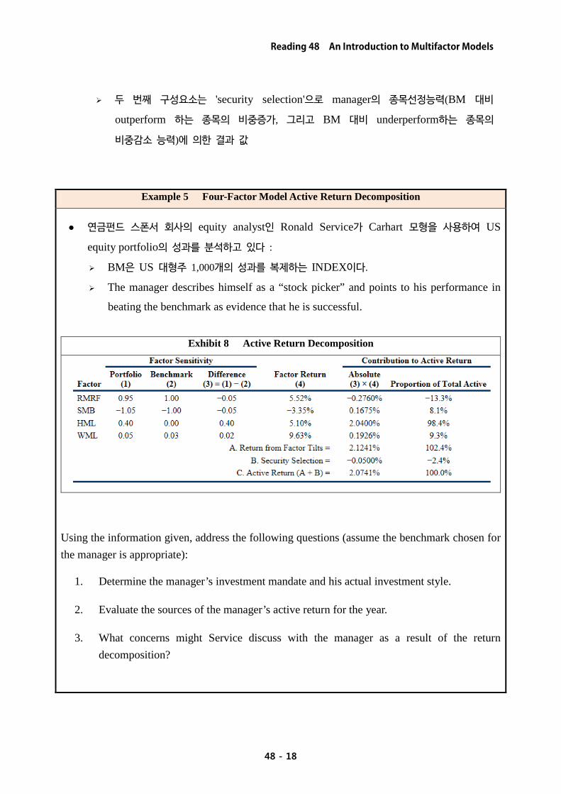
Example 5 Four-Factor Model Active Return Decomposition

연금펀드 스폰서 회사의 equity analyst인 Ronald Service가 Carhart 모형을 사용하여 US

equity portfolio의 성과를 분석하고 있다 :

BM은 US 대형주 1,000개의 성과를 복제하는 INDEX이다.

The manager describes himself as a “stock picker” and points to his performance in

beating the benchmark as evidence that he is successful.

Exhibit 8 Active Return Decomposition

Using the information given, address the following questions (assume the benchmark chosen for the manager is appropriate):

1. Determine the manager’s investment mandate and his actual investment style.

2. Evaluate the sources of the manager’s active return for the year.

3. What concerns might Service discuss with the manager as a result of the return decomposition?


48 - 19

Solution to 1

BM의 RMRF factor에 대한 sensitivity가 1 이므로 전반적인 시장지수의 특성을 반영하고

있고 미국 대형주 1,000개의 성과를 복제하고자 하는 BM의 설정에 부합된다. 또한 SMB

factor의 sensitivity가 -1이므로 대형주 중심이다.

The mandate might be described as large-cap without a value/growth bias (HML is

zero) or a momentum bias (WML is close to zero).

portfolio가 HML에 대해 0.4의 sensitivity를 보유하고 있으므로 value orientation으로

파악될 수 있고, WML은 거의 zero에 가까우므로 momentum과 contrarian에 대해서는

중립적이다.

In summary, the above considerations suggest that the manager has a large-cap value

orientation.

Solution to 2

Manager의 positive active return에 가장 중요한 원천은 HML factor에 대한 positive

exposure이다.

Solution to 3

Manager가 스스로를 "stock picker"로 표현하고 있지만, security selection 효과가

negative이기 때문에 이는 부적절한 표현이다.


48 - 20

5.2 Factor Models in Risk Attribution

Active risk는 active return의 표준편차이다.

TE(tracking error)라고도 하며 CFA커리큘럼에서는 tracking risk로 표현한다.

포트폴리오 수익률 RP와 BM의 수익률 RB의 차이에 대한 시계열 자료에 의한 sample

표준편차로서 TE는 다음과 같다 :

TE = S (RP - RB) (8)

미국 주식시장에서 TE 값은 (1) well-executed passive investment strategy : 0.10%,

(2) low-risk active or enhanced index investment strategy : 2%, (3) diversified large-cap equity strategy : 2%-6%, (4) aggressive active equity manager : 6%-10%

정도이다.

IR(information ratio)

Somewhat analogous to the use of the traditional Sharpe measure in evaluating

absolute returns, the information ratio (IR) is a tool for evaluating mean active

returns per unit of active risk. The historical or ex post IR is expressed as follows:

IR = )( BP

BP

RRRR−−

s (9)

PR 와 BR 는 각각 포트폴리오의 sample mean return과 BM의 sample mean return을

나타낸다.

특정기간 동안에 포트폴리오가 평균수익률 9%, BM은 평균수익률 7.5%, TE가 6%라면,

IR = (9% - 7.5%) / 6% = 0.25 이다.


48 - 21

Example 6 Creating Active Manager Guidelines

'active return'과 'active risk'는 투자위험을 관리하고자 하는 투자자에게 유용한 분석체계이다.

잘 알려져 있고 지속적으로 관찰 가능한 벤치마크를 비교기준으로 활용하여, 계량적 위험과

수익률 목적을 상대적으로 표현하고 소통할 수 있다. For example, a US public employee retirement system invited investment managers to submit proposals to manage a “low-active-risk US large-cap equity fund” that would be subject to the following constraints: Shares must be components of the S&P 500. The portfolio should have a minimum of 200 issues. At time of purchase, the

maximum amount that may be invested in any one issuer is 5% of the portfolio at market value or 150% of the issuers’ weight within the S&P 500, whichever is greater.

The portfolio must have a minimum information ratio of 0.30 either since inception or over the last seven years.

The portfolio must also have tracking risk of less than 3% with respect to the S&P 500 either since inception or over the last seven years.

적합한 active manager가 선정되면, 이들 요구사항들이 '운용사에 대한 지침'에 문서화될 수

있다. retirement system의 운용사 개별 mandate들은 모든 mandate들을 합산했을 때 그것이

'desired risk exposure'가 될 수 있도록 구성된다.

성과분석 analyst들은 multifactor 모형을 사용하여 active manager의 risk exposure를

상세하게 이해하고자 한다. 즉 tracking error의 원천을 이해하고 다음사항에 대한 이해를

얻고자 하는 것이다 :

Manager TE에 가장 크게 공헌한 risk exposure는 무엇인가?

Manager는 자신의 active exposure의 성격을 깨닫고 있는가? 만일 그렇다면, 그러한

위험감수에 대한 합리성을 잘 설명할 수 있는가?

포트폴리오의 active risk exposure는 manager가 내세우고 있는 투자철학과 부합되고

있는가?

어떤 active bet이 감수한 active risk 수준에 충분한 수익률을 창출하였는가?

성과분석 analyst들은 가장 직접적이고 직관적인 방법으로 active risk exposure를

manager의 포트폴리오 의사결정과 연결시킬 수 있으므로 주로 fundamental factor 모형을

사용하여 분석한다.


48 - 22

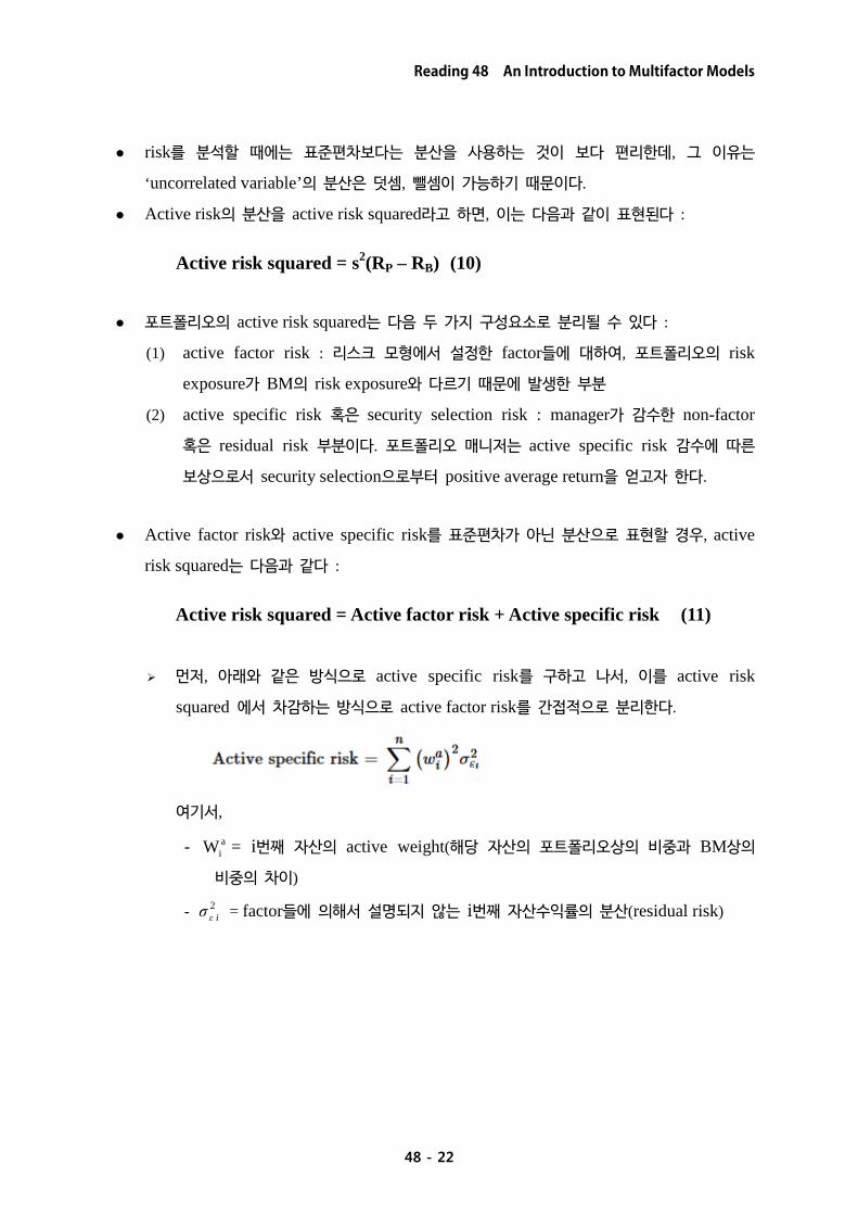
risk를 분석할 때에는 표준편차보다는 분산을 사용하는 것이 보다 편리한데, 그 이유는

‘uncorrelated variable’의 분산은 덧셈, 뺄셈이 가능하기 때문이다.

Active risk의 분산을 active risk squared라고 하면, 이는 다음과 같이 표현된다 :

Active risk squared = s2(RP – RB) (10)

포트폴리오의 active risk squared는 다음 두 가지 구성요소로 분리될 수 있다 :

(1) active factor risk : 리스크 모형에서 설정한 factor들에 대하여, 포트폴리오의 risk

exposure가 BM의 risk exposure와 다르기 때문에 발생한 부분

(2) active specific risk 혹은 security selection risk : manager가 감수한 non-factor

혹은 residual risk 부분이다. 포트폴리오 매니저는 active specific risk 감수에 따른

보상으로서 security selection으로부터 positive average return을 얻고자 한다.

Active factor risk와 active specific risk를 표준편차가 아닌 분산으로 표현할 경우, active

risk squared는 다음과 같다 :

Active risk squared = Active factor risk + Active specific risk (11)

먼저, 아래와 같은 방식으로 active specific risk를 구하고 나서, 이를 active risk

squared 에서 차감하는 방식으로 active factor risk를 간접적으로 분리한다.

여기서,

- aiW = i번째 자산의 active weight(해당 자산의 포트폴리오상의 비중과 BM상의

비중의 차이)

- 2iεσ = factor들에 의해서 설명되지 않는 i번째 자산수익률의 분산(residual risk)


48 - 23

Example 7 A Comparison of Active Risk

Richard Gray가 동일한 BM을 공유하는 네 개의 equity manager에 대한 active risk 분석을

수행한다.

BARRA US-E4 model : 12개의 style factor와 60개의 industry factor로 구성된

fundamental multifactor model을 사용한다.

Style factor는 size, liquidity, leverage, 그리고 dividend yield 등으로 구성

Exhibit 9 Active Risk Squared Decomposition

Note : Entries are in % squared.

Using the information in Exhibit 9, address the following:

Contrast the active risk decomposition of Portfolios A and B.

Contrast the active risk decomposition of Portfolios B and C.

Characterize the investment approach of Portfolio D.

Solution to 1

Exhibit 10 Active Risk Decomposition (re-stated)


48 - 24

Portfolio A는 B에 비해 높은 수준의 active risk를 감수했다(7% versus 5%)

Portfolio A와 B는 active factor와 active specific 비중면에서는 동일하지만, active

factor 내에서의 세부 비중은 크게 차이가 난다.

Portfolio A는 상대적으로 active industry risk를, Portfolio B는 industry에 대해서는

중립적인 반면, style factor risk를 보다 많이 감수했다.

Solution to 2

Portfolio B와 C는 active risk의 절대적인 수준이 유사하고 industry neutral 특성을

나타내고 있다.

Portfolio C는 높은 active factor risk를, Portfolio B는 높은 active specific risk를

감수했다.

Portfolio B의 active specific risk가 상대적으로 큰 것으로 보아, C에 비해 less

diversified 되어 있다고 추정할 수 있다.

Solution to 3

Portfolio D appears to be a passively managed portfolio, judging by its negligible level of active risk.


48 - 25

5.3. Factor Models in Portfolio Construction

Portfolio management process 중 portfolio 구축단계에서 multifactor 모형은 포트폴리오

manager가 BM risk와 비교하여 의도한 비중선택(focused bet)을 하거나 portfolio risk를

통제할 수 있도록 도와준다.

Risk를 modeling함에 있어서 multifactor 모형이 제공할 수 있는 상당한 수준의

섬세함은 passive management와 active management 모두에 유용하다.

passive management : 추정하고자 하는 index fund의 factor exposure를 정확하게

복제하는데 활용한다.

active management : alpha를 얻기 위해 원하는 risk profile을 수립하기 위해 사용한다.

rule-based active management(alternative indexes) : 포트폴리오를 구축할 때

정규적으로 size, value, quality 혹은 momentum 등의 요인들에 대해 BM과 다른

비중선택을 시도한다. Alternative index strategies rely heavily on factor models to

introduce intentional factor and style biases versus capitalization-weighted indexes.


48 - 26

Example 8 Factor Portfolios

애널리스트 Wanda Smithfield는 회사에서 포트폴리오 매니저가 사용할 수 있는 여섯 개의

포트폴리오 A, B, C, D, E, F를 구축하여 Exhibit 11에 제시하고 있다. Smithfield는 Burmeister,

Roll, and Ross(1994)의 연구에서 제시한 macroeconomic factor 모형을 수정해서 개발하였다. 이

모형은 다음과 같은 다섯 개의 factor를 사용하고 있다 :

Confidence risk, based on the yield spread between corporate bonds and government bonds. A positive surprise in the spread suggests that investors are willing to accept a smaller reward for bearing default risk and so that confidence is high.

Time horizon risk, based on the yield spread between 20-year government bonds and 30-day Treasury bills. A positive surprise indicates increased investor willingness to invest for the long term.

Inflation risk, measured by the unanticipated change in the inflation rate. Business cycle risk, measured by the unexpected change in the level of real

business activity. Market timing risk, measured as the portion of the return on a broad-based

equity index that is unexplained by the first four risk factors.

Exhibit 11 Factor Portfolios

Note : Entries are factor sensitivities.

1. A portfolio manager wants to place a bet that real business activity will increase.

A. Determine and justify the portfolio among the six given that would be most useful to the manager.

B. Would the manager take a long or short position in the portfolio chosen in Part A?


48 - 27

2. A portfolio manager wants to hedge an existing positive (long) exposure to time horizon risk.

A. Determine and justify the portfolio among the six given that would be most useful to the manager.

B. What type of position would the manager take in the portfolio chosen in Part A?

Solution to 1A

Portfolio B가 적절한 선택이다. Portfolio B는 business cycle risk에 대해서만 민감도가 1 이고

다른 모든 factor들에 대해서는 민감도가 0 이므로 'factor portfolio' 이다. 따라서 실질경기가

좋아질 것이라는 요소에만 순수하게 bet하는데 효율적으로 사용할 수 있다. Solution to 1B Portfolio B 에 long position을 취한다.

Solution to 2A Portfolio D가 time horizon risk에 대한 pure factor portfolio이므로, 적합한 선택이다. Solution to 2B

Portfolio D 에 short position을 취한다


48 - 28

5.4. How Factor Considerations Can Be Useful in Strategic Portfolio Decisions

multifactor 모형은 투자자들이 여러 전략적 의사결정을 수행함에 있어서 관련된

고려사항들을 인식하는데 도움을 준다.

가령, 자산의 평균수익률에 영향을 미치는 체계적 위험요인에 대한 훌륭한 model이

있다면, 투자자들은 본인들이 다른 투자자에 비해 상대적인 비교우위를 갖는 위험의

종류와 비교열위에 있는 위험의 종류를 파악할 수 있을 것이다.

예를 들어, university endowment(대학기금)는 business cycle risk나 private equity

같은 liquidity risk를 감수하는데 있어서 비교우위가 있다.

This is a richer framework than that afforded by the CAPM, according to which all

investors optimally should invest in two funds: the market portfolio and a risk-free

asset.

A multifactor approach can help investors achieve better-diversified and possibly more

efficient portfolios.

For example, the characteristics of a portfolio can be better explained by a

combination of SMB, HML, and WML factors in addition to the market factor than

by using the market factor alone.

Thus, compared with single-factor models, multifactor models offer a richer

context for investors to search for ways to improve portfolio selection.


48 - 29

1. Compare the assumptions of the arbitrage pricing theory (APT) with those of the capital asset pricing model (CAPM).

2. Last year the return on Harry Company stock was 5 percent. The portion of the return on the stock not explained by a two-factor macroeconomic factor model was 3 percent. Using the data given below, calculate Harry Company stock’s expected return.

Macroeconomic Factor Model for Harry Company Stock

3. Assume that the following one-factor model describes the expected return for

portfolios:

E(Rp) = 0.10 + 0.12βp,1

Also assume that all investors agree on the expected returns and factor sensitivity of the three highly diversified Portfolios A, B, and C given in the following table:

Assuming the one-factor model is correct and based on the data provided for Portfolios A, B, and C, determine if an arbitrage opportunity exists and explain how it might be exploited.

PROBLEMS


48 - 30

4. Which type of factor model is most directly applicable to an analysis of the style orientation (for example, growth vs. value) of an active equity investment manager? Justify your answer.

5. Suppose an active equity manager has earned an active return of 110 basis points, of which 80 basis points is the result of security selection ability. Explain the likely source of the remaining 30 basis points of active return.

6. Address the following questions about the information ratio.

What is the information ratio of an index fund that effectively meets its investment

objective?


48 - 31

SOLUTION

1. APT와 CAPM은 모두 "위험자산이 균형상태에서 위험에 대해 요구하는 수익률(장기 기대

수익률)"을 설명하는 모형이다. CAPM은 [투자자는 수익률의 평균(mean), 분산(variance),

상관관계(correlation)만을 고려하여 포트폴리오 결정을 할 수 있다]는 가정을 포함한 일련의

가정을 전제하고 있다. The APT makes three assumptions :

A. A factor model describes asset returns. B. There are many assets, so investors can form well-diversified portfolios that

eliminate asset-specific risk. C. No arbitrage opportunities exist among well-diversified portfolios.

2. macroeconomic factor 모형에서 어느 factor에 대한 기대차이(surprise)는 실제 값에서 기대

값을 뺀 것이다. interest rate factor에 대한 surprise는 2%, GDP factor에 대한 surprise는

-3%가 된다. 이 모형에서 상수(절편)는 최초의 기대수익률이며, 모형에 의해 설명되지 않는

수익률 부분이 error term이다.

5% = Expected return – 1.5(Interest rate surprise) + 2(GDP surprise) + Error term = Expected return – 1.5(2%) + 2(–3%) + 3% = Expected return – 6%

Rearranging terms, the expected return for Harry Company stock equals ; 5% + 6% = 11%.

3. According to the one-factor model for expected returns, the portfolio should have these expected returns if they are correctly priced in terms of their risk:

Portfolio A : E(RA) = 0.10 + 0.12βA,1 = 0.10 + (0.12)(0.80) = 0.10 + 0.10 = 0.20

Portfolio B : E(RB) = 0.10 + 0.12βB,1 = 0.10 + (0.12)(1.00) = 0.10 + 0.12 = 0.22

Portfolio C : E(RC) = 0.10 + 0.12βC,1 = 0.10 + (0.12)(1.20) = 0.10 + 0.14 = 0.24

아래 표에서 Portfolio A와 C의 기대수익률은 모형에 의한 위험평가를 정확하게 반영하고

있지만, Portfolio B는 모형에 의한 기대수익률 보다 낮은 15% 수익률을 제시하고 있다.

따라서 고평가된 Portfolio B(기대수익률이 낮다는 것은 가격이 높다는 뜻이다)를 shorting

하고 수령한 금액으로 A와 C에 각각 50%씩 투자하는 포트폴리오를 매입한다.


48 - 32

'50% A + 50% C' 포트폴리오의 민감도는 1로서 portfolio B와 동일하게 대응된다.

이러한 €1 arbitrage 투자전략에 의해, 확정된 profit €0.07(=0.22 - 0.15)를 확보하게 된다.

4. A fundamental factor model. Such models typically include many factors related to the company (e.g., earnings) and to valuation that are commonly used indicators of a growth orientation. A macroeconomic factor model may provide relevant information as well, but typically indirectly and in less detail.

5. 나머지 30 basis point 수익률은 factor tilt에 따른 것이다.

포트폴리오 manager의 active return은 'factor tilt'와 'security selection' 두 요소의 합이다.

'factor tile'란 운용자가 BM과 비교하여 상대적으로 높거나 낮은 factor sensitivity를 선택함에

따라 발생한 차이에 factor return을 곱하여 합산한 결과이다.

'security selection'은 outperform할 유가증권을 overweight하고, underform할 유가증권을

underweight하는 운용자의 능력을 반영한다.

6. An index fund that effectively meets its investment objective is expected to have an information ratio of zero, because its active return should be zero.

READING An Introduction to Multifactor Models 48wkedu.co.kr/widget/img/data/Reading 48(2018...

Documents

Transcript of READING An Introduction to Multifactor Models 48wkedu.co.kr/widget/img/data/Reading 48(2018...