RC Model Aircraft Design Analysis Notes

Notes and Formulas Useful In Analyzing the Performance of Model Aircraft

William B. Garner

Rev 2, December 2018

Rev 1 Notes: Revised Aircraft Lift and Drag section, adding measurement units for metric and English systems Expanded drag equations to include fuselage and tail contributions Removed or modified most formulas containing English units Corrected several errors

Rev2 Notes: There is some minor editing, clarification of some measurement units, correction of formula for Moment.

Provides notes and formulas for the evaluation of model aircraft performance. Subjects included are aerodynamics, propellers and electric power systems.

1

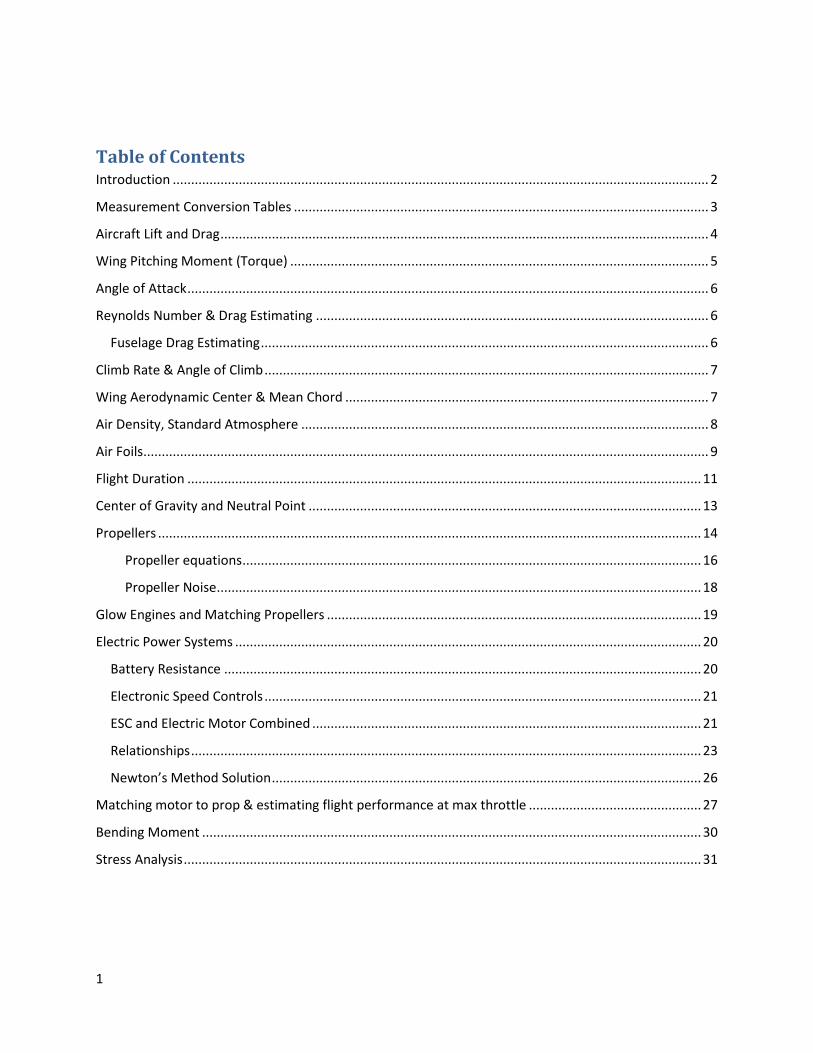
Table of Contents Introduction .................................................................................................................................................. 2

Measurement Conversion Tables ................................................................................................................. 3

Aircraft Lift and Drag ..................................................................................................................................... 4

Wing Pitching Moment (Torque) .................................................................................................................. 5

Angle of Attack .............................................................................................................................................. 6

Reynolds Number & Drag Estimating ........................................................................................................... 6

Fuselage Drag Estimating .......................................................................................................................... 6

Climb Rate & Angle of Climb ......................................................................................................................... 7

Wing Aerodynamic Center & Mean Chord ................................................................................................... 7

Air Density, Standard Atmosphere ............................................................................................................... 8

Air Foils .......................................................................................................................................................... 9

Flight Duration ............................................................................................................................................ 11

Center of Gravity and Neutral Point ........................................................................................................... 13

Propellers .................................................................................................................................................... 14

Propeller equations ............................................................................................................................. 16

Propeller Noise .................................................................................................................................... 18

Glow Engines and Matching Propellers ...................................................................................................... 19

Electric Power Systems ............................................................................................................................... 20

Battery Resistance .................................................................................................................................. 20

Electronic Speed Controls ....................................................................................................................... 21

ESC and Electric Motor Combined .......................................................................................................... 21

Relationships ........................................................................................................................................... 23

Newton’s Method Solution ..................................................................................................................... 26

Matching motor to prop & estimating flight performance at max throttle ............................................... 27

Bending Moment ........................................................................................................................................ 30

Stress Analysis ............................................................................................................................................. 31

2

Introduction Over the years I have collected a number of programs and descriptions related to the design and performance of RC model airplanes. They are scattered in various books, notebooks, document files and computer programs, making finding some particular subject sometimes a challenge. This document attempts to remedy that condition by assembling a lot of them in one place. It is limited to a set of subjects that are of most interest to the author. Topics included are various aspects of aerodynamics, propellers and electric power systems. There is a section on in-flight performance combining the aerodynamics and electric power system to estimate flight duration as a function of power setting as well as climb performance. The subjects are mostly presented without explanations as to their use or derivations. It is assumed the reader has some understanding of these subjects and does not need further explanations. Many of the explanations can be found in the literature, but there are a few that the author developed for a specific purpose. The section on in-flight performance was developed by the author and does contain some more detailed explanations. The application of the formulas and other information requires the use of a consistent set of measurement units. Any set can be used. Tables are included giving conversions from ft-lb-sec system to the metric system. The formulas and other types of numerical information are approximations to the real world. For instance, wing profile drag coefficients change with air speed and angle of attack but it is very difficult to include these changes in any straight forward analysis. The result is that there are differences between computed results and actual results that can be quite large. It makes no sense, then, to carry out computations to 3 decimal places when the actual results may be no better than no decimal places. There are three books that were especially helpful in understanding how models work and perform. #1: Lennon, Andy, “R/C Model Aircraft Design”, Air Age, Inc., 2002. The best source for detailed explanations of just about every RC airplane subject with math models for many of them. Much of the formulae in this document came from this source. #2: Simmons, Martin; “Model Aircraft Dynamics”, Fourth Edition, Special Interest Model Books, Dorset, UK, 2002. More qualitative than quantitative, many excellent chapters on the underlying principles of aerodynamics as applied to models. There is a large appendix devoted to airfoils and one with example calculations of aerodynamic properties. #3: Smith, H.C. ‘Skip”, “The Illustrated Guide to Aerodynamics”, 2nd Edition, 1992, Tab Books (McGraw Hill), This book was written for a private pilot so is written in a more general manner than the other books. It has lots of illustrations and photos that help in understanding the descriptions. It is a good starting book.

3

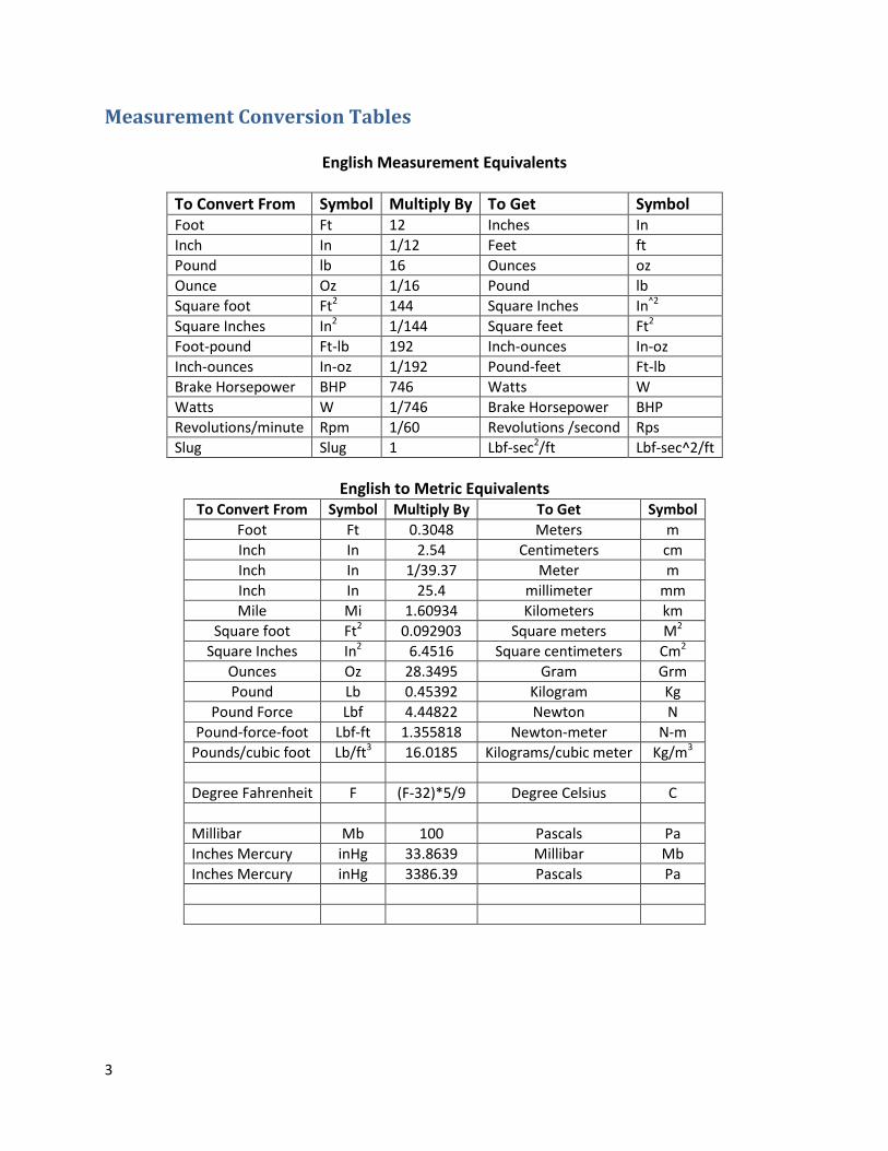
Measurement Conversion Tables

English Measurement Equivalents

To Convert From Symbol Multiply By To Get Symbol Foot Ft 12 Inches In

Inch In 1/12 Feet ft

Pound lb 16 Ounces oz

Ounce Oz 1/16 Pound lb

Square foot Ft2 144 Square Inches In^2

Square Inches In2 1/144 Square feet Ft2

Foot-pound Ft-lb 192 Inch-ounces In-oz

Inch-ounces In-oz 1/192 Pound-feet Ft-lb

Brake Horsepower BHP 746 Watts W

Watts W 1/746 Brake Horsepower BHP

Revolutions/minute Rpm 1/60 Revolutions /second Rps

Slug Slug 1 Lbf-sec2/ft Lbf-sec^2/ft

English to Metric Equivalents To Convert From Symbol Multiply By To Get Symbol

Foot Ft 0.3048 Meters m

Inch In 2.54 Centimeters cm

Inch In 1/39.37 Meter m

Inch In 25.4 millimeter mm

Mile Mi 1.60934 Kilometers km

Square foot Ft2 0.092903 Square meters M2

Square Inches In2 6.4516 Square centimeters Cm2

Ounces Oz 28.3495 Gram Grm

Pound Lb 0.45392 Kilogram Kg

Pound Force Lbf 4.44822 Newton N

Pound-force-foot Lbf-ft 1.355818 Newton-meter N-m

Pounds/cubic foot Lb/ft3 16.0185 Kilograms/cubic meter Kg/m3

Degree Fahrenheit F (F-32)*5/9 Degree Celsius C

Millibar Mb 100 Pascals Pa

Inches Mercury inHg 33.8639 Millibar Mb

Inches Mercury inHg 3386.39 Pascals Pa

4

Aircraft Lift and Drag

Symbol Description Metric Units British Units

b Wing Span m ft

Cl Lift Coefficient

Cdi Wing Induced Drag Coefficient

Cdw Wing Profile Drag Coefficient

Cdf Fuselage Drag Coefficient

Cdt Tail Drag Coefficient

g Gravity Constant 9.81 m/sec^2 32.2 ft/sec^2

h Height above sea level m ft

L Lift Force Kg-m/sec^2 Lb-ft/sec^2

Drag Drag Force Kg-m/sec^2 Lb-ft/sec^2

W Mass Kg Lb

P Power, Watts Kg-m^2/sec^3 1.356*Lb-ft^2/sec^3

V Air Speed m/sec ft/sec

Sw Wing Area m^2 ft^2

Sf Fuselage Effective Drag Area m^2 ft^2

St Tail Area m^2 ft^2

ρo Air Density at Sea Level 1.225 Kg/m^3 0.00765 Lb/ft^3

σ Air Density Correction for Height Above Sea Level

1-8.245E-05*h 1-2.519e-05*h

ρ Air Density = ρo*σ Kg/m^3 Lb/ft^3

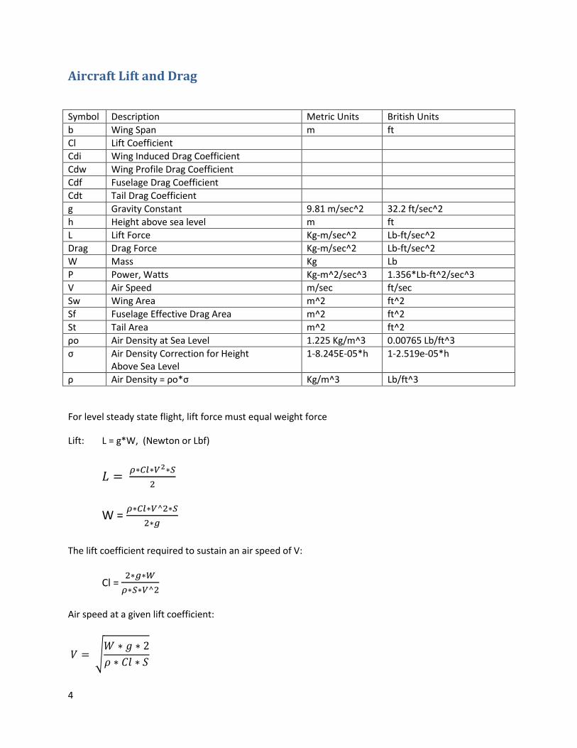
For level steady state flight, lift force must equal weight force

Lift: L = g*W, (Newton or Lbf)

W =

The lift coefficient required to sustain an air speed of V:

Cl =

Air speed at a given lift coefficient:

√

5

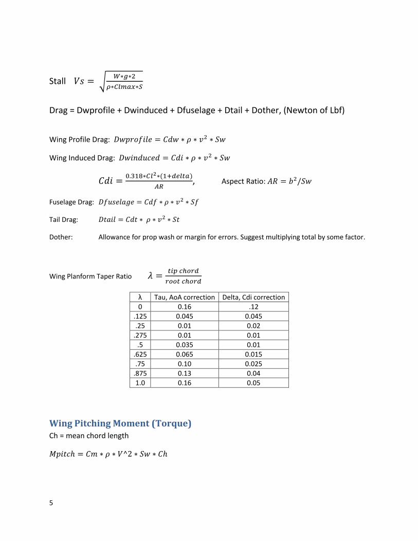
Stall √

Drag = Dwprofile + Dwinduced + Dfuselage + Dtail + Dother, (Newton of Lbf)

Wing Profile Drag:

Wing Induced Drag:

, Aspect Ratio:

Fuselage Drag:

Tail Drag:

Dother: Allowance for prop wash or margin for errors. Suggest multiplying total by some factor.

Wing Planform Taper Ratio

λ Tau, AoA correction Delta, Cdi correction

0 0.16 .12

.125 0.045 0.045

.25 0.01 0.02

.275 0.01 0.01

.5 0.035 0.01

.625 0.065 0.015

.75 0.10 0.025

.875 0.13 0.04

1.0 0.16 0.05

Wing Pitching Moment (Torque) Ch = mean chord length

6

Angle of Attack The actual angle of attack is a function of the lift coefficient, wing planform and the aspect ratio.

Α0 is angle of attack from airfoil infinite aspect ratio plot at given Cl.

Degrees

Reynolds Number & Drag Estimating

Re =

=

V is the fluid velocity L is the characteristic length, the chord width of an airfoil ρ is the fluid density μ is the dynamic fluid viscosity v is the kinematic fluid viscosity

v = 1.511E-05, m^2/sec at sea level

v = 1.626E-04, ft^2/sec at sea level

Divide v by σ for other altitudes.

A tapered wing has chords that decrease in length from root to tip. This means that the Reynolds number decreases in proportion and the corresponding drag coefficient increases. The drag area will decrease with chord decrease, and since drag is proportional to area and drag coefficient, the net drag change is not all that great. A compromise to calculating the drag at stations along the span and adding them is to use the mean aerodynamic chord length in the drag estimation.

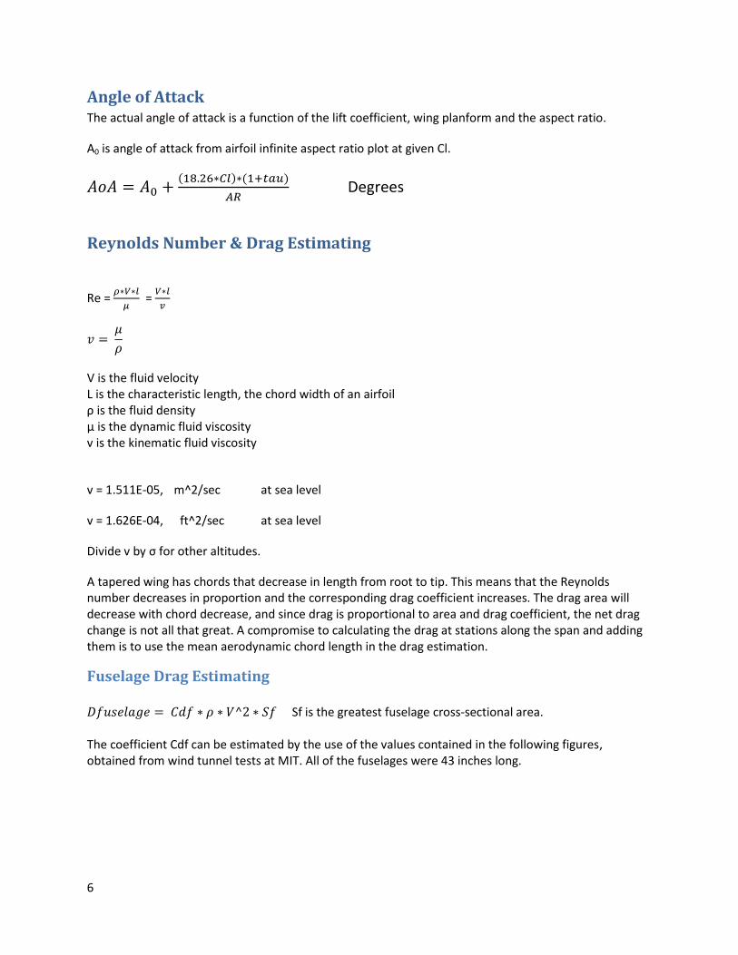
Fuselage Drag Estimating Sf is the greatest fuselage cross-sectional area. The coefficient Cdf can be estimated by the use of the values contained in the following figures, obtained from wind tunnel tests at MIT. All of the fuselages were 43 inches long.

7

Note that other combinations can be derived from these results. For instance, fuselages 1 and 8 are the same except that number 8 has landing gear. The increase in the coefficient is thus due to the landing gear.

Climb Rate & Angle of Climb

,

(

) , degrees

If thrust > drag then Climb Angle = 900

Wing Aerodynamic Center & Mean Chord Assumes uniform tapered wing, dimensions in inches R = root chord T = tip chord

8

Span = distance from root to tip (half of total wing span) Sweep = distance tip leading edge is swept back from root leading edge MAC = mean aerodynamic chord AC = aerodynamic center measured from root leading edge

(area of wing half)

Air Density, Standard Atmosphere Assumes standard temperature and pressure conditions at sea level. There is no allowance for actual

temperature or water vapor-caused variations.

po = sea level standard atmospheric pressure, 101.325 kPa

To = sea level standard temperature, 288.15 K

g = earth surface gravitational acceleration, 9.80665 m/s2

L = Temperature lapse rate, 0.0065, K/m

R = Ideal gas constant, 8.31447 J/(mol-K)

M = molar mass of dry air, 0.0289644 kg/mol

Temperature at altitude h meters above sea level:

T = To – L*h

The pressure at altitude h is given by:

(

)

Density then is found to be:

Kg/m3

9

This set of equations is essentially linear with altitude.

,Kg/m3

σ =

= 1- 8.24E-05*hmeter

Air Foils

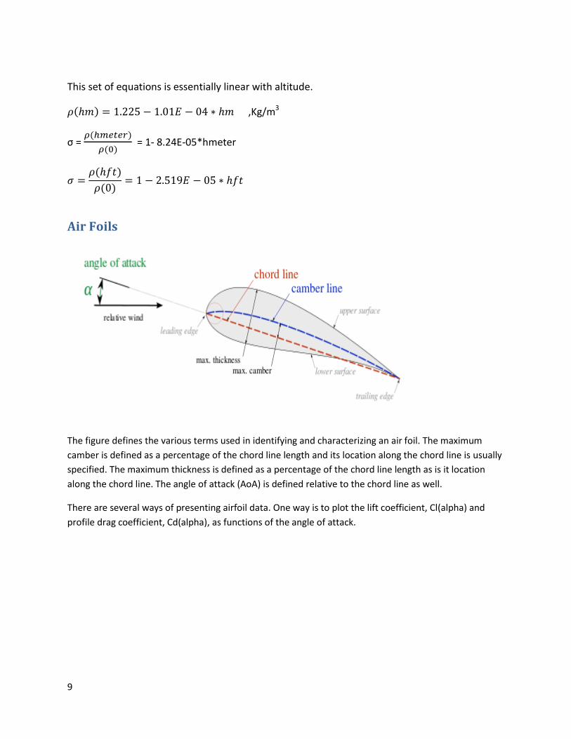
The figure defines the various terms used in identifying and characterizing an air foil. The maximum

camber is defined as a percentage of the chord line length and its location along the chord line is usually

specified. The maximum thickness is defined as a percentage of the chord line length as is it location

along the chord line. The angle of attack (AoA) is defined relative to the chord line as well.

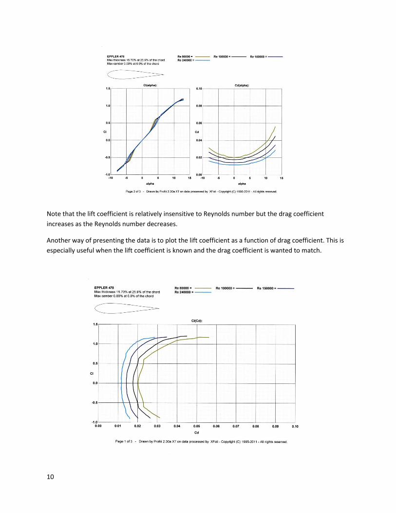
There are several ways of presenting airfoil data. One way is to plot the lift coefficient, Cl(alpha) and

profile drag coefficient, Cd(alpha), as functions of the angle of attack.

10

Note that the lift coefficient is relatively insensitive to Reynolds number but the drag coefficient

increases as the Reynolds number decreases.

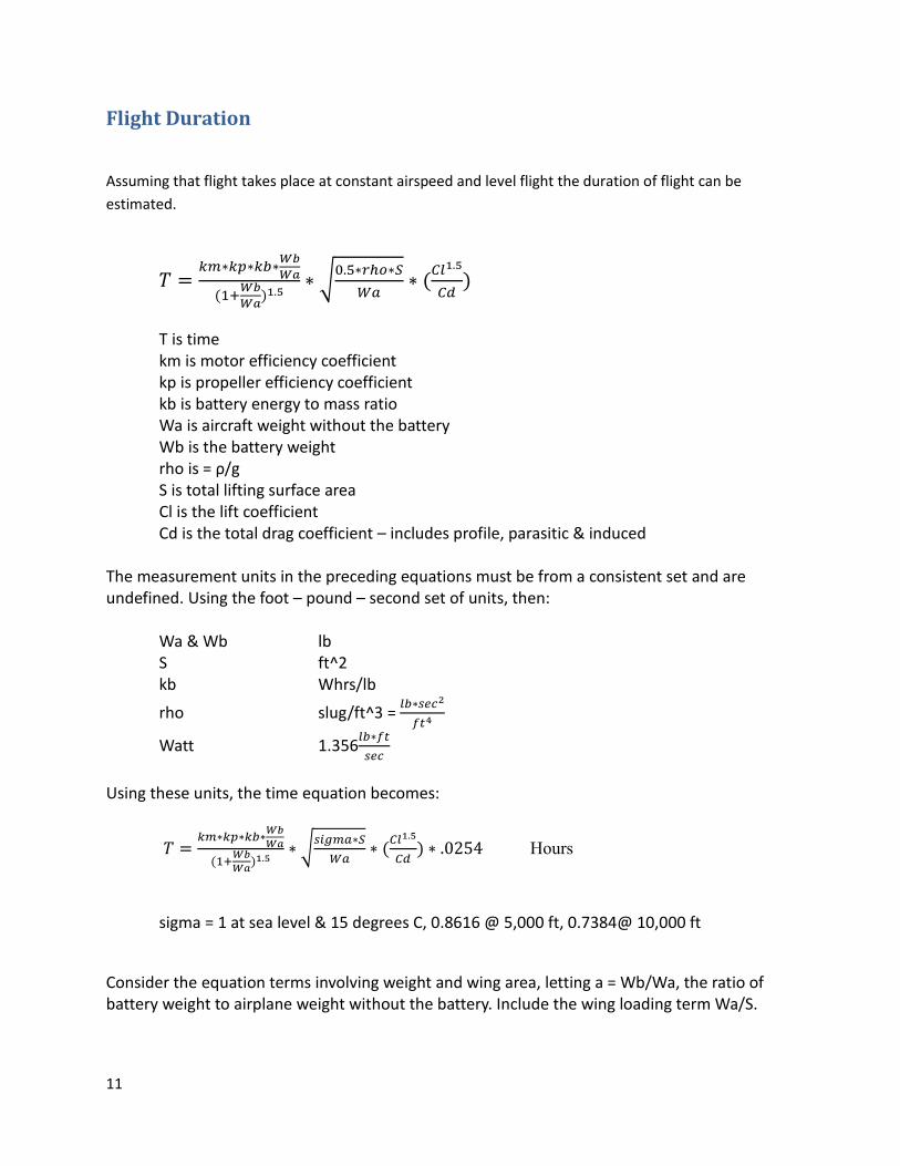
Another way of presenting the data is to plot the lift coefficient as a function of drag coefficient. This is

especially useful when the lift coefficient is known and the drag coefficient is wanted to match.

11

Flight Duration

Assuming that flight takes place at constant airspeed and level flight the duration of flight can be

estimated.

𝑘 𝑘 𝑘

𝑊𝑏

𝑊𝑎

𝑊𝑏

𝑊𝑎 1 5

√ 5

1 5

T is time km is motor efficiency coefficient kp is propeller efficiency coefficient kb is battery energy to mass ratio Wa is aircraft weight without the battery Wb is the battery weight rho is = ρ/g S is total lifting surface area Cl is the lift coefficient Cd is the total drag coefficient – includes profile, parasitic & induced The measurement units in the preceding equations must be from a consistent set and are undefined. Using the foot – pound – second set of units, then: Wa & Wb lb S ft^2 kb Whrs/lb

rho slug/ft^3 =

𝑓 4

Watt 1.356 𝑓

Using these units, the time equation becomes:

𝑘 𝑘 𝑘

𝑊𝑏

𝑊𝑎

𝑊𝑏

𝑊𝑎 1 5

√

1 5

Hours

sigma = 1 at sea level & 15 degrees C, 0.8616 @ 5,000 ft, 0.7384@ 10,000 ft

Consider the equation terms involving weight and wing area, letting a = Wb/Wa, the ratio of battery weight to airplane weight without the battery. Include the wing loading term Wa/S.

12

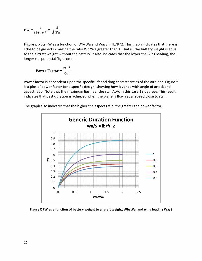
FW =

1 5 √

Figure x plots FW as a function of Wb/Wa and Wa/S In lb/ft^2. This graph indicates that there is little to be gained in making the ratio Wb/Wa greater than 1. That is, the battery weight is equal to the aircraft weight without the battery. It also indicates that the lower the wing loading, the longer the potential flight time.

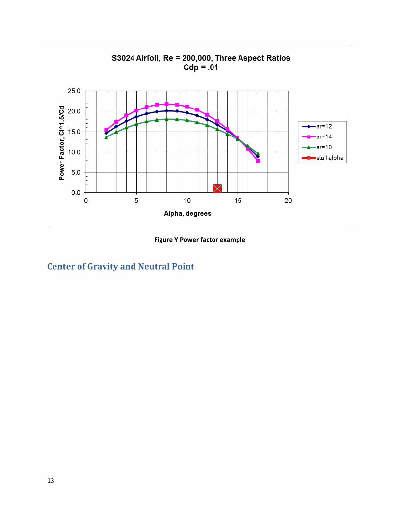
Power Factor = 1 5

Power factor is dependent upon the specific lift and drag characteristics of the airplane. Figure Y is a plot of power factor for a specific design, showing how it varies with angle of attack and aspect ratio. Note that the maximum lies near the stall AoA, in this case 13 degrees. This result indicates that best duration is achieved when the plane is flown at airspeed close to stall. The graph also indicates that the higher the aspect ratio, the greater the power factor.

Figure X FW as a function of battery weight to aircraft weight, Wb/Wa, and wing loading Wa/S

13

Figure Y Power factor example

Center of Gravity and Neutral Point

14

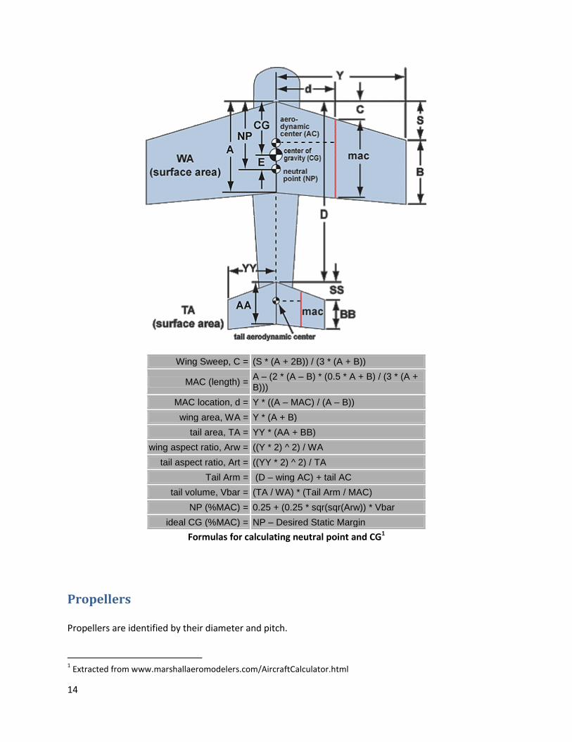
Wing Sweep, C = (S * (A + 2B)) / (3 * (A + B))

MAC (length) = A – (2 * (A – B) * (0.5 * A + B) / (3 * (A + B)))

MAC location, d = Y * ((A – MAC) / (A – B))

wing area, WA = Y * (A + B)

tail area, TA = YY * (AA + BB)

wing aspect ratio, Arw = ((Y * 2) ^ 2) / WA

tail aspect ratio, Art = ((YY * 2) ^ 2) / TA

Tail Arm = (D – wing AC) + tail AC

tail volume, Vbar = (TA / WA) * (Tail Arm / MAC)

NP (%MAC) = 0.25 + (0.25 * sqr(sqr(Arw)) * Vbar

ideal CG (%MAC) = NP – Desired Static Margin

Formulas for calculating neutral point and CG1

Propellers Propellers are identified by their diameter and pitch.

1 Extracted from www.marshallaeromodelers.com/AircraftCalculator.html

15

Pitch is the hypothetical distance forward a propeller would advance in one revolution if there were no

slippage.

Pitch is measured relative to the chord line, normally at 70 to 75% of the blade radius.

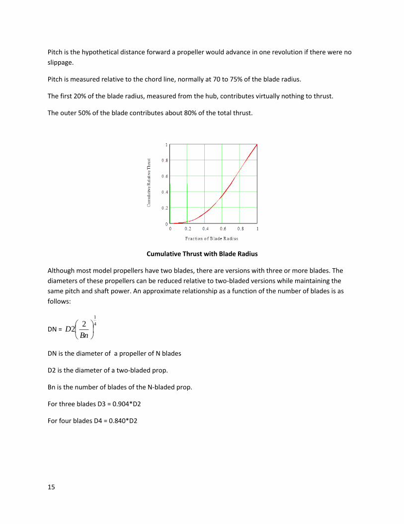
The first 20% of the blade radius, measured from the hub, contributes virtually nothing to thrust.

The outer 50% of the blade contributes about 80% of the total thrust.

Cumulative Thrust with Blade Radius

Although most model propellers have two blades, there are versions with three or more blades. The

diameters of these propellers can be reduced relative to two-bladed versions while maintaining the

same pitch and shaft power. An approximate relationship as a function of the number of blades is as

follows:

DN = 4

1

22

BnD

DN is the diameter of a propeller of N blades

D2 is the diameter of a two-bladed prop.

Bn is the number of blades of the N-bladed prop.

For three blades D3 = 0.904*D2

For four blades D4 = 0.840*D2

16

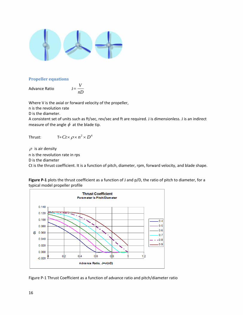
Propeller equations

Advance Ratio JnD

V

Where V is the axial or forward velocity of the propeller, n is the revolution rate D is the diameter. A consistent set of units such as ft/sec, rev/sec and ft are required. J is dimensionless. J is an indirect

measure of the angle at the blade tip.

Thrust: T= 42 DnCt

is air density

n is the revolution rate in rps D is the diameter Ct is the thrust coefficient. It is a function of pitch, diameter, rpm, forward velocity, and blade shape.

Figure P-1 plots the thrust coefficient as a function of J and p/D, the ratio of pitch to diameter, for a typical model propeller profile

Figure P-1 Thrust Coefficient as a function of advance ratio and pitch/diameter ratio

17

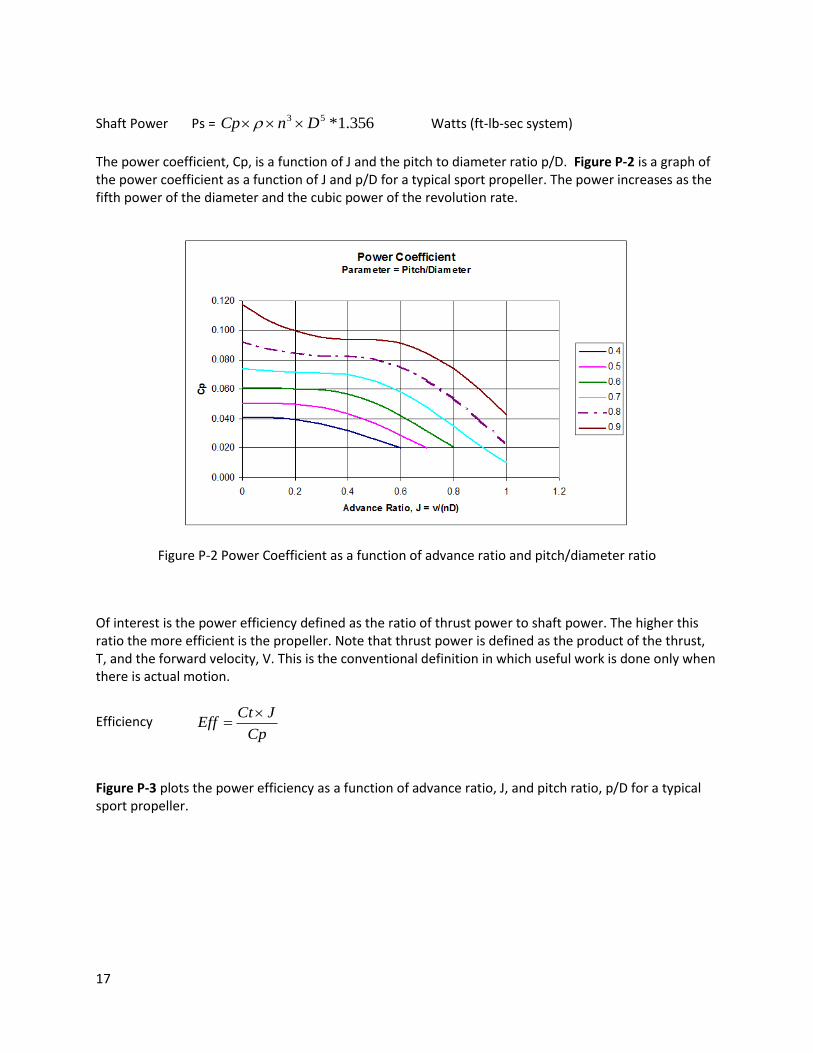
Shaft Power Ps = 356.1*53 DnCp Watts (ft-lb-sec system)

The power coefficient, Cp, is a function of J and the pitch to diameter ratio p/D. Figure P-2 is a graph of the power coefficient as a function of J and p/D for a typical sport propeller. The power increases as the fifth power of the diameter and the cubic power of the revolution rate.

Figure P-2 Power Coefficient as a function of advance ratio and pitch/diameter ratio

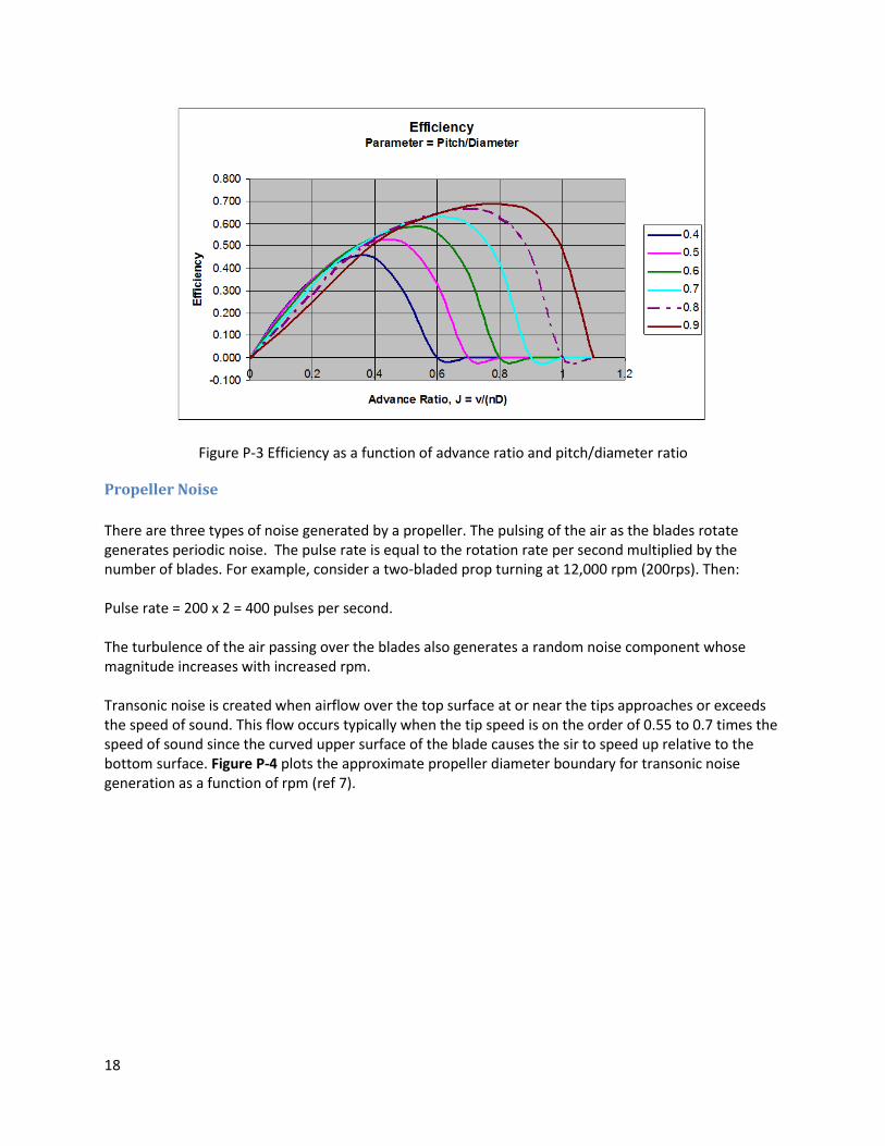
Of interest is the power efficiency defined as the ratio of thrust power to shaft power. The higher this ratio the more efficient is the propeller. Note that thrust power is defined as the product of the thrust, T, and the forward velocity, V. This is the conventional definition in which useful work is done only when there is actual motion.

Efficiency Cp

JCtEff

Figure P-3 plots the power efficiency as a function of advance ratio, J, and pitch ratio, p/D for a typical sport propeller.

18

Figure P-3 Efficiency as a function of advance ratio and pitch/diameter ratio

Propeller Noise

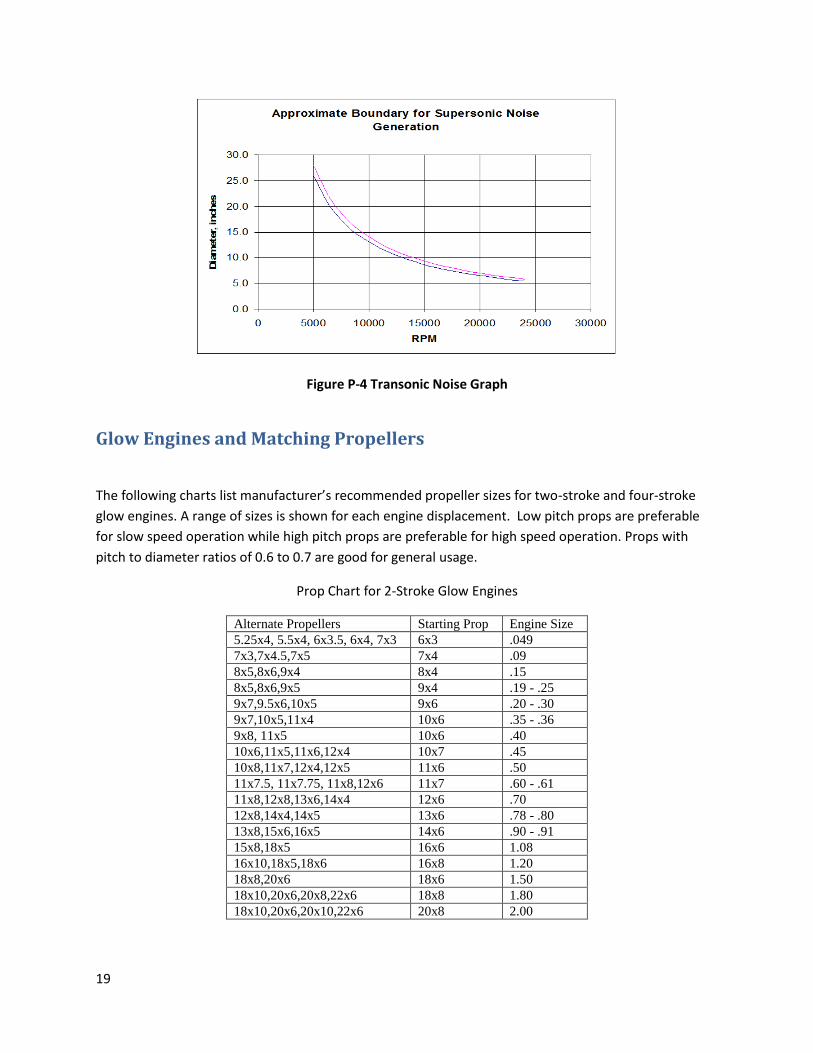
There are three types of noise generated by a propeller. The pulsing of the air as the blades rotate generates periodic noise. The pulse rate is equal to the rotation rate per second multiplied by the number of blades. For example, consider a two-bladed prop turning at 12,000 rpm (200rps). Then: Pulse rate = 200 x 2 = 400 pulses per second. The turbulence of the air passing over the blades also generates a random noise component whose magnitude increases with increased rpm. Transonic noise is created when airflow over the top surface at or near the tips approaches or exceeds the speed of sound. This flow occurs typically when the tip speed is on the order of 0.55 to 0.7 times the speed of sound since the curved upper surface of the blade causes the sir to speed up relative to the bottom surface. Figure P-4 plots the approximate propeller diameter boundary for transonic noise generation as a function of rpm (ref 7).

19

Figure P-4 Transonic Noise Graph

Glow Engines and Matching Propellers

The following charts list manufacturer’s recommended propeller sizes for two-stroke and four-stroke

glow engines. A range of sizes is shown for each engine displacement. Low pitch props are preferable

for slow speed operation while high pitch props are preferable for high speed operation. Props with

pitch to diameter ratios of 0.6 to 0.7 are good for general usage.

Prop Chart for 2-Stroke Glow Engines

Alternate Propellers Starting Prop Engine Size

5.25x4, 5.5x4, 6x3.5, 6x4, 7x3 6x3 .049

7x3,7x4.5,7x5 7x4 .09

8x5,8x6,9x4 8x4 .15

8x5,8x6,9x5 9x4 .19 - .25

9x7,9.5x6,10x5 9x6 .20 - .30

9x7,10x5,11x4 10x6 .35 - .36

9x8, 11x5 10x6 .40

10x6,11x5,11x6,12x4 10x7 .45

10x8,11x7,12x4,12x5 11x6 .50

11x7.5, 11x7.75, 11x8,12x6 11x7 .60 - .61

11x8,12x8,13x6,14x4 12x6 .70

12x8,14x4,14x5 13x6 .78 - .80

13x8,15x6,16x5 14x6 .90 - .91

15x8,18x5 16x6 1.08

16x10,18x5,18x6 16x8 1.20

18x8,20x6 18x6 1.50

18x10,20x6,20x8,22x6 18x8 1.80

18x10,20x6,20x10,22x6 20x8 2.00

20

Prop Chart for Four-Stroke Glow Engines

Alternate Propellers Starting Prop Engine Size

9x5,10x5 9x6 .20 - .21

10x6,10x7,11x4,11x5.11x7,11x7.

5,12x4,12x5

11x6 .40

10x6,10x7,10x8,11x7,11x7.5,12x

4,12x5,12x6

11x6 .45 - .48

11x7.5,11x7.75,11x8,12x8,13x5,

13x6,14x5,14x6

12x6 .60 - .65

12x8,13x8,14x4,14x6 13x6 .80

13x6,14x8,15x6,16x6 14x6 .90

14x8,15x6,15x8,16x8,17x6,18x5,

18x6

16x6 1.20

15x6,15x8,16x8,18x6,18x8,20x6 18x6 1.60

18x12,20x8,20x10 18x10 2.40

18x10,18x12,20x10 20x8 2.70

18x12,20x10 20x10 3.00

Electric Power Systems

Battery Resistance

Battery resistance is used in estimating the performance of RC electric power systems. The following

formula is useful for that purpose. It assumes that the battery is new as used batteries may have

substantially higher internal resistance.

5

, Ohms

Ncells is the number of cells in series

AH is the ampere hour rating

C is the c-rating. Multiply it times the Amp Hours to get maximum current draw.

21

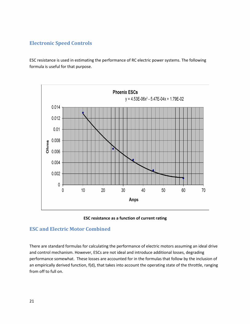
Electronic Speed Controls

ESC resistance is used in estimating the performance of RC electric power systems. The following

formula is useful for that purpose.

ESC resistance as a function of current rating

ESC and Electric Motor Combined

There are standard formulas for calculating the performance of electric motors assuming an ideal drive

and control mechanism. However, ESCs are not ideal and introduce additional losses, degrading

performance somewhat. These losses are accounted for in the formulas that follow by the inclusion of

an empirically derived function, f(d), that takes into account the operating state of the throttle, ranging

from off to full on.

22

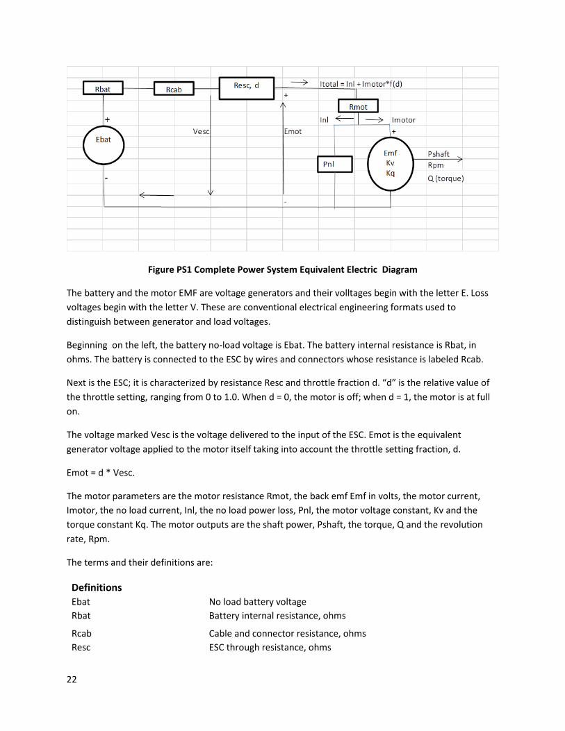
Figure PS1 Complete Power System Equivalent Electric Diagram

The battery and the motor EMF are voltage generators and their volltages begin with the letter E. Loss

voltages begin with the letter V. These are conventional electrical engineering formats used to

distinguish between generator and load voltages.

Beginning on the left, the battery no-load voltage is Ebat. The battery internal resistance is Rbat, in

ohms. The battery is connected to the ESC by wires and connectors whose resistance is labeled Rcab.

Next is the ESC; it is characterized by resistance Resc and throttle fraction d. “d” is the relative value of

the throttle setting, ranging from 0 to 1.0. When d = 0, the motor is off; when d = 1, the motor is at full

on.

The voltage marked Vesc is the voltage delivered to the input of the ESC. Emot is the equivalent

generator voltage applied to the motor itself taking into account the throttle setting fraction, d.

Emot = d * Vesc.

The motor parameters are the motor resistance Rmot, the back emf Emf in volts, the motor current,

Imotor, the no load current, Inl, the no load power loss, Pnl, the motor voltage constant, Kv and the

torque constant Kq. The motor outputs are the shaft power, Pshaft, the torque, Q and the revolution

rate, Rpm.

The terms and their definitions are:

Definitions Ebat

No load battery voltage

Rbat

Battery internal resistance, ohms

Rcab Cable and connector resistance, ohms

Resc

ESC through resistance, ohms

23

Rmot

Motor internal resistance, ohms

Pnl

Motor power loss due to internal non resistive causes

Emf

Motor back EMF, opposed to the battery voltage, volts

Pshaft

Power output through the motor shaft

Kv

Motor rpm per volt

Io

no load reference current at Vo

Vo

no load reference voltage

Inl

Motor no load current, Amps

Imot

Motor current transferring power to the output shaft, Amps

d Fraction of full throttle setting, range 0 to 1.0

Emot

The source voltage driving the motor from the ESC, Volts

Relationships

There are some relationships that are common to all working formulas that follow.

f(d) = 1+d*(1-d) ESC loss factor, multiplied by the motor current. Vesc = Ebat –Itotal*(Rbat + Rcab + Resc) Voltage into ESC Emotor= d*Vesc Voltage out of ESC to motor, viewed as a generator Inl = (Io/Vo)*Emf No load current, Amps Pnl = Inl*Emf No load power, Watts Itotal = Inl + Imot*f(d) Total current, Amps Emf = Kv * Rpm Motor back voltage, Volts Kq = 1353/Kv Torque constant, in-oz. /Amp Q = Kq*Imot Torque, in-oz. Pshaft = Imot* Emf Shaft power, Watts Case1: Assume that the throttle is at its full position and the motor is stalled such that the rpm is zero. Under these conditions the full battery voltage is applied to the motor and only the resistances impede the flow of current. As an example, assume that the battery voltage is 11 Volts and the total resistance is 0.15 ohms in a small motor rated 20 Amps and 1000 Kv. The current is then 11V/.15Ohms = 73 Amps, enough to severely damage the ESC, motor or battery. The torque would be 73*1353/1000 = 98 in- oz. If a finger or piece of clothing were the cause of the stalled condition, the torque would be such that real damage could occur. Case 2: A second case is to estimate the torque, rpm, shaft power and battery power by varying the current. This approach is fairly common in displaying the characteristics of a specific motor.

24

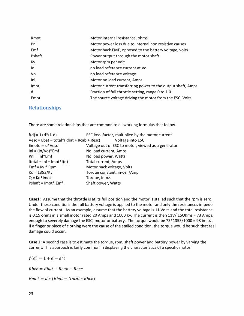
Example result for half-throttle setting

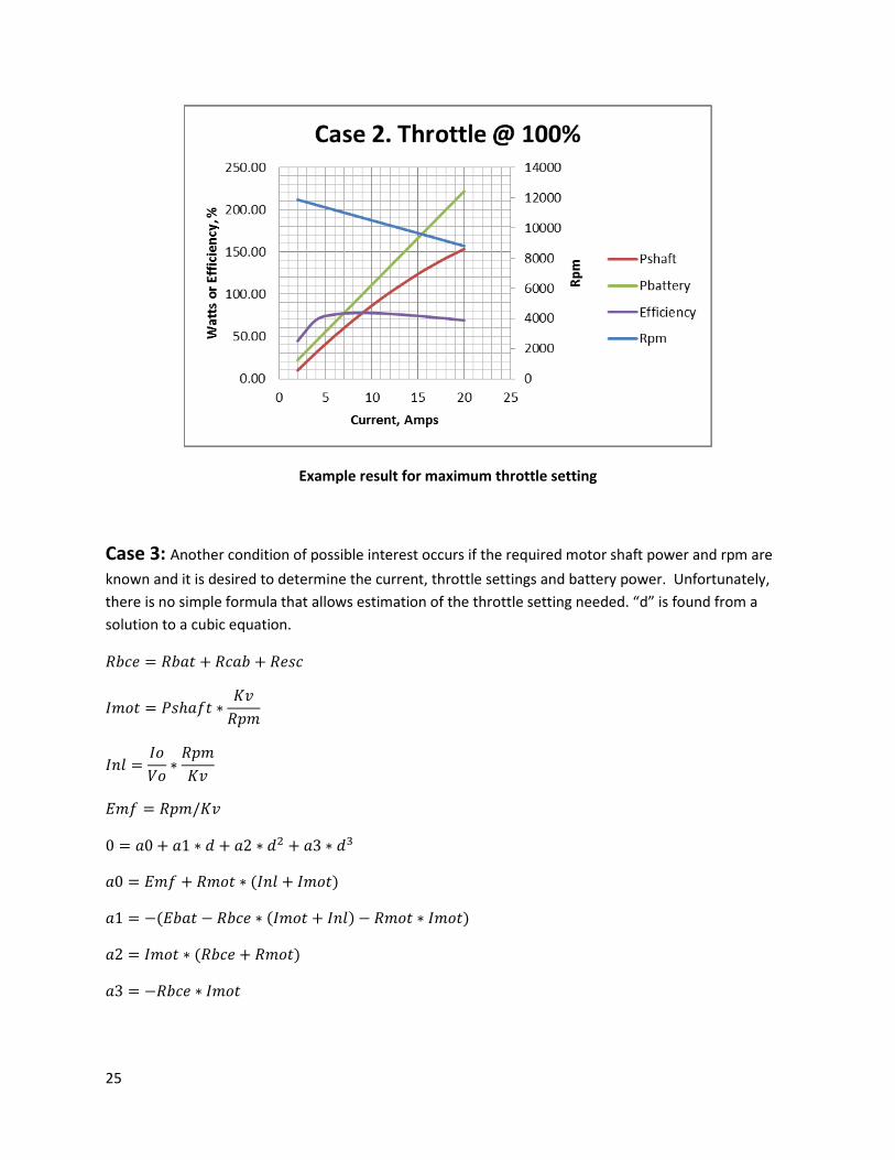
The battery power increases linearly with current. The shaft power increases linearly at low currents,

then slowly bends over as the internal losses increase more rapidly. The rpm decreases as the load

increases, the efficiency is low at low currents, increase rapidly then flattens out with increases in

current.

25

Example result for maximum throttle setting

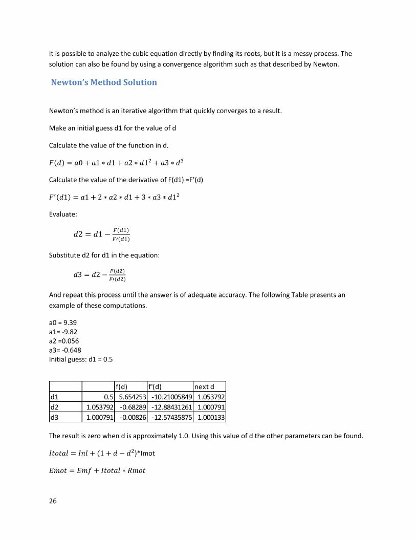
Case 3: Another condition of possible interest occurs if the required motor shaft power and rpm are

known and it is desired to determine the current, throttle settings and battery power. Unfortunately,

there is no simple formula that allows estimation of the throttle setting needed. “d” is found from a

solution to a cubic equation.

26

It is possible to analyze the cubic equation directly by finding its roots, but it is a messy process. The

solution can also be found by using a convergence algorithm such as that described by Newton.

Newton’s Method Solution

Newton’s method is an iterative algorithm that quickly converges to a result.

Make an initial guess d1 for the value of d

Calculate the value of the function in d.

Calculate the value of the derivative of F(d1) =F’(d)

Evaluate:

Substitute d2 for d1 in the equation:

And repeat this process until the answer is of adequate accuracy. The following Table presents an

example of these computations.

a0 = 9.39 a1= -9.82 a2 =0.056 a3= -0.648 Initial guess: d1 = 0.5

The result is zero when d is approximately 1.0. Using this value of d the other parameters can be found.

)*Imot

f(d) f'(d) next d

d1 0.5 5.654253 -10.21005849 1.053792

d2 1.053792 -0.68289 -12.88431261 1.000791

d3 1.000791 -0.00826 -12.57435875 1.000133

27

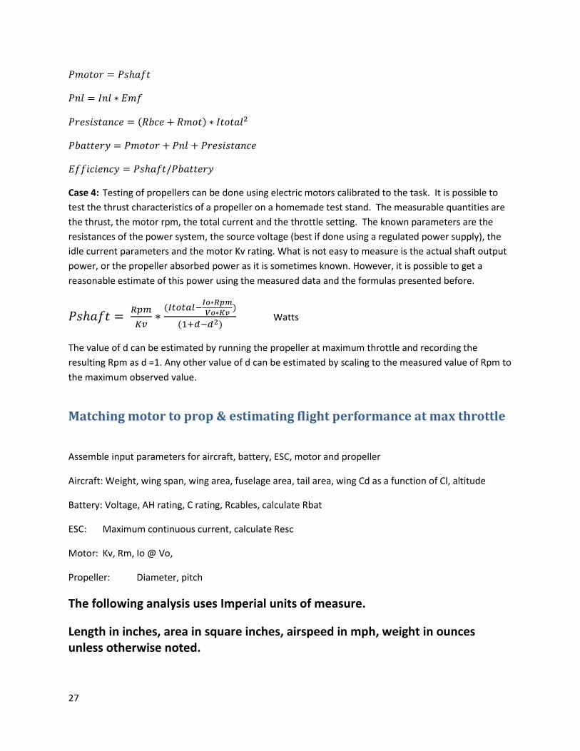
Case 4: Testing of propellers can be done using electric motors calibrated to the task. It is possible to

test the thrust characteristics of a propeller on a homemade test stand. The measurable quantities are

the thrust, the motor rpm, the total current and the throttle setting. The known parameters are the

resistances of the power system, the source voltage (best if done using a regulated power supply), the

idle current parameters and the motor Kv rating. What is not easy to measure is the actual shaft output

power, or the propeller absorbed power as it is sometimes known. However, it is possible to get a

reasonable estimate of this power using the measured data and the formulas presented before.

Watts

The value of d can be estimated by running the propeller at maximum throttle and recording the

resulting Rpm as d =1. Any other value of d can be estimated by scaling to the measured value of Rpm to

the maximum observed value.

Matching motor to prop & estimating flight performance at max throttle

Assemble input parameters for aircraft, battery, ESC, motor and propeller

Aircraft: Weight, wing span, wing area, fuselage area, tail area, wing Cd as a function of Cl, altitude

Battery: Voltage, AH rating, C rating, Rcables, calculate Rbat

ESC: Maximum continuous current, calculate Resc

Motor: Kv, Rm, Io @ Vo,

Propeller: Diameter, pitch

The following analysis uses Imperial units of measure.

Length in inches, area in square inches, airspeed in mph, weight in ounces unless otherwise noted.

28

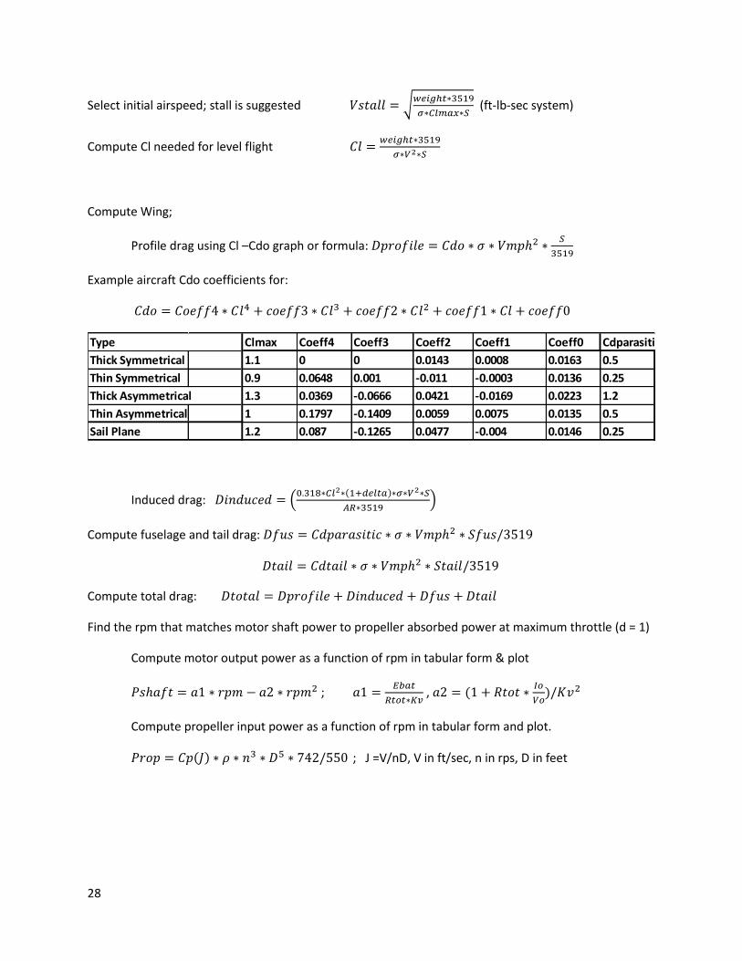
Select initial airspeed; stall is suggested √ 5

(ft-lb-sec system)

Compute Cl needed for level flight 5

Compute Wing;

Profile drag using Cl –Cdo graph or formula:

5

Example aircraft Cdo coefficients for:

Induced drag: (

5 )

Compute fuselage and tail drag:

Compute total drag:

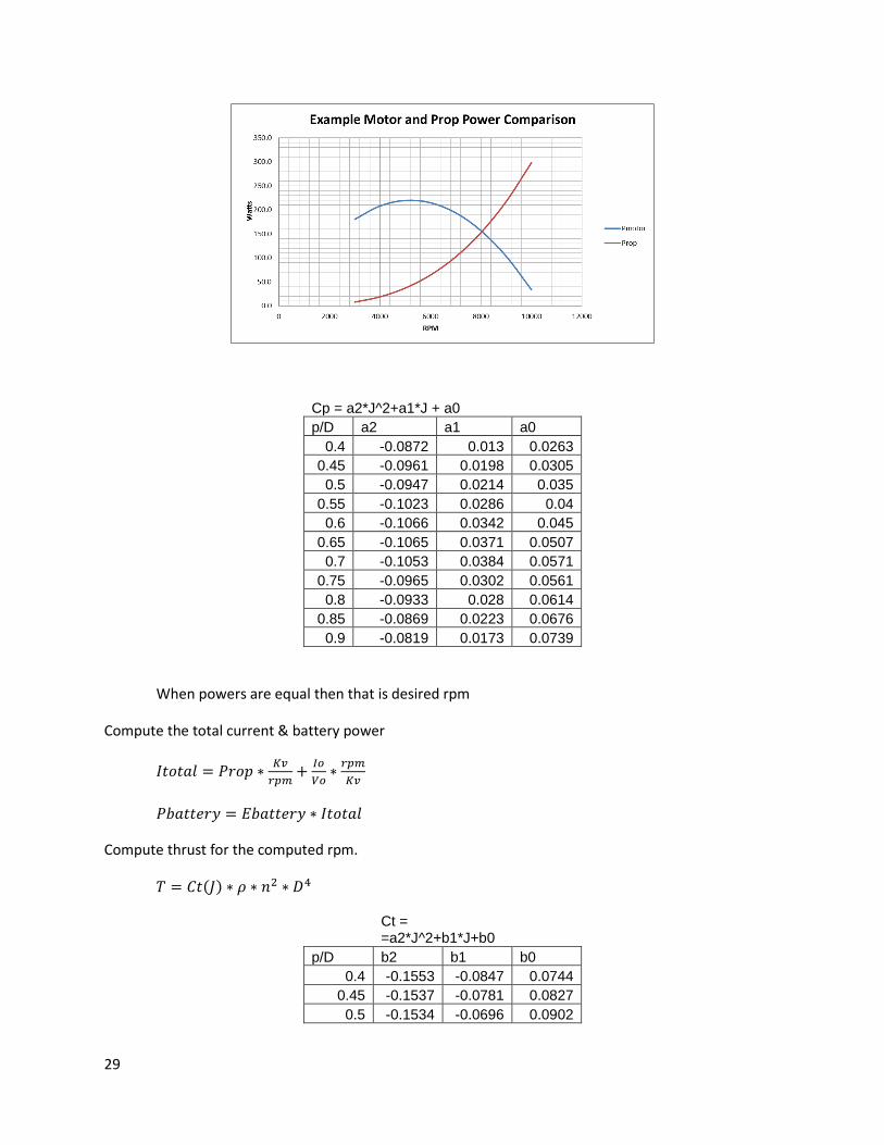
Find the rpm that matches motor shaft power to propeller absorbed power at maximum throttle (d = 1)

Compute motor output power as a function of rpm in tabular form & plot

;

,

Compute propeller input power as a function of rpm in tabular form and plot.

5 ; J =V/nD, V in ft/sec, n in rps, D in feet

Clmax Coeff4 Coeff3 Coeff2 Coeff1 Coeff0 Cdparasitic

Thick Symmetrical 1.1 0 0 0.0143 0.0008 0.0163 0.5

Thin Symmetrical 0.9 0.0648 0.001 -0.011 -0.0003 0.0136 0.25

Thick Asymmetrical 1.3 0.0369 -0.0666 0.0421 -0.0169 0.0223 1.2

Thin Asymmetrical 1 0.1797 -0.1409 0.0059 0.0075 0.0135 0.5

Sail Plane 1.2 0.087 -0.1265 0.0477 -0.004 0.0146 0.25

Type

29

Cp = a2*J^2+a1*J + a0 p/D a2 a1 a0

0.4 -0.0872 0.013 0.0263

0.45 -0.0961 0.0198 0.0305

0.5 -0.0947 0.0214 0.035

0.55 -0.1023 0.0286 0.04

0.6 -0.1066 0.0342 0.045

0.65 -0.1065 0.0371 0.0507

0.7 -0.1053 0.0384 0.0571

0.75 -0.0965 0.0302 0.0561

0.8 -0.0933 0.028 0.0614

0.85 -0.0869 0.0223 0.0676

0.9 -0.0819 0.0173 0.0739

When powers are equal then that is desired rpm

Compute the total current & battery power

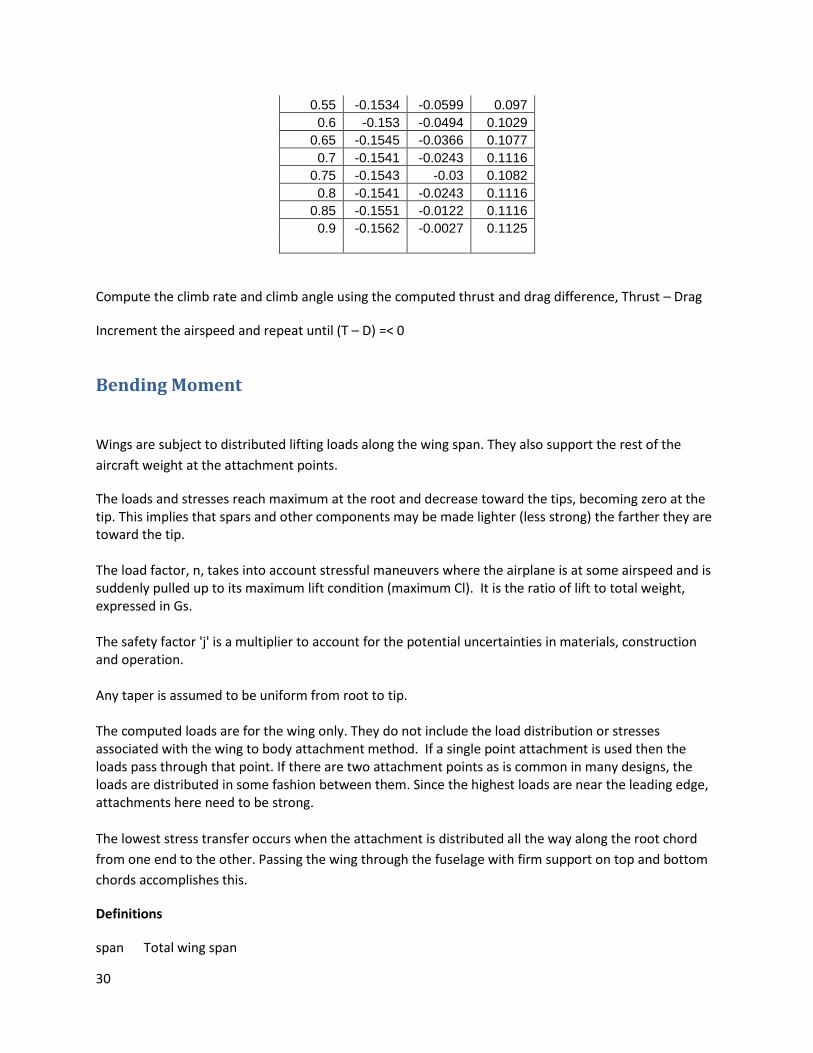
Compute thrust for the computed rpm.

Ct = =a2*J^2+b1*J+b0

p/D b2 b1 b0

0.4 -0.1553 -0.0847 0.0744

0.45 -0.1537 -0.0781 0.0827

0.5 -0.1534 -0.0696 0.0902

30

0.55 -0.1534 -0.0599 0.097

0.6 -0.153 -0.0494 0.1029

0.65 -0.1545 -0.0366 0.1077

0.7 -0.1541 -0.0243 0.1116

0.75 -0.1543 -0.03 0.1082

0.8 -0.1541 -0.0243 0.1116

0.85 -0.1551 -0.0122 0.1116

0.9 -0.1562 -0.0027 0.1125

Compute the climb rate and climb angle using the computed thrust and drag difference, Thrust – Drag

Increment the airspeed and repeat until (T – D) =< 0

Bending Moment

Wings are subject to distributed lifting loads along the wing span. They also support the rest of the

aircraft weight at the attachment points.

The loads and stresses reach maximum at the root and decrease toward the tips, becoming zero at the tip. This implies that spars and other components may be made lighter (less strong) the farther they are toward the tip. The load factor, n, takes into account stressful maneuvers where the airplane is at some airspeed and is suddenly pulled up to its maximum lift condition (maximum Cl). It is the ratio of lift to total weight, expressed in Gs. The safety factor 'j' is a multiplier to account for the potential uncertainties in materials, construction and operation. Any taper is assumed to be uniform from root to tip. The computed loads are for the wing only. They do not include the load distribution or stresses associated with the wing to body attachment method. If a single point attachment is used then the loads pass through that point. If there are two attachment points as is common in many designs, the loads are distributed in some fashion between them. Since the highest loads are near the leading edge, attachments here need to be strong.

The lowest stress transfer occurs when the attachment is distributed all the way along the root chord

from one end to the other. Passing the wing through the fuselage with firm support on top and bottom

chords accomplishes this.

Definitions

span Total wing span

31

cr Wing root chord

ct Wing tip chord

Qw Wing weight

Qt Total aircraft weight

Clmax Maximum wing lift coefficient

Vmax Maximum airspeed

J Safety factor

Bending Moment Equations

Wing semi-span

,

Semi-span area

,

Load Factor

Gs

Semi-span load

Tip load intensity

,

Root load intensity

,

Root Moment

,

Root vertical load

,

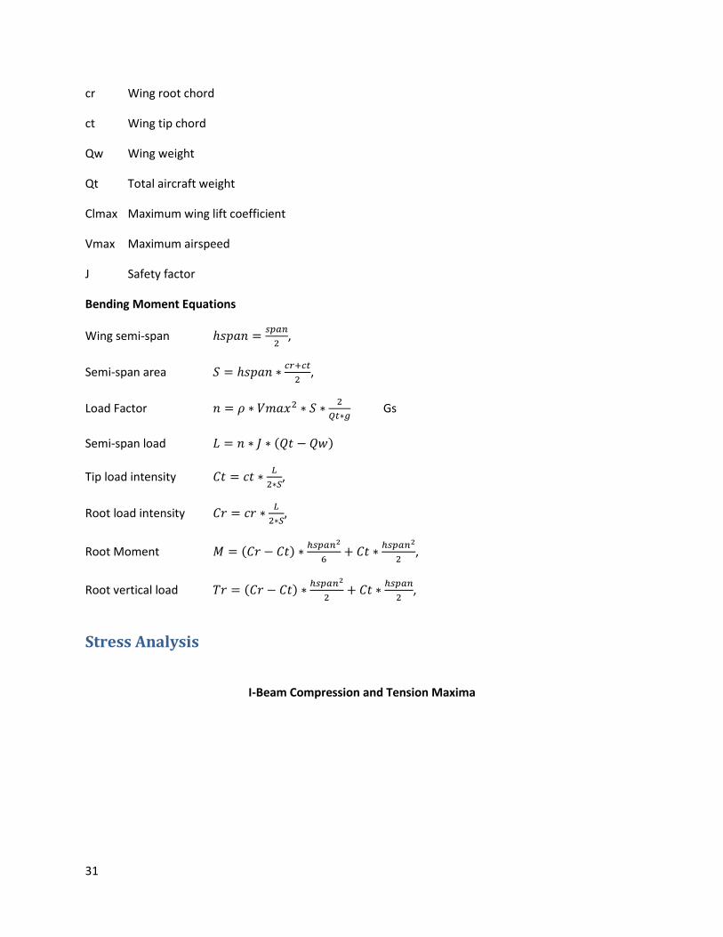
Stress Analysis

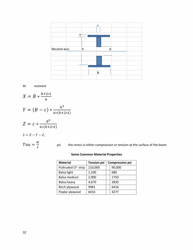
I-Beam Compression and Tension Maxima

32

M moment

,

psi the stress in either compression or tension at the surface of the beam

Some Common Material Properties

Material Tension psi Compression psi

Pultruded CF strip 110,000 90,000

Balsa light 1,100 680

Balsa medium 2,900 1750

Balsa heavy 4,670 2830

Birch plywood 9981 6416

Poplar plywood 6416 4277

c

t

Neutral axis h d

B