Rayleigh-gravity waves in a heavy elastic medium

Kuipers, M.; van de Ven, A.A.F.

Published: 01/01/1989

Document VersionPublisher’s PDF, also known as Version of Record (includes final page, issue and volume numbers)

Please check the document version of this publication:

• A submitted manuscript is the author's version of the article upon submission and before peer-review. There can be important differencesbetween the submitted version and the official published version of record. People interested in the research are advised to contact theauthor for the final version of the publication, or visit the DOI to the publisher's website.• The final author version and the galley proof are versions of the publication after peer review.• The final published version features the final layout of the paper including the volume, issue and page numbers.

Link to publication

General rightsCopyright and moral rights for the publications made accessible in the public portal are retained by the authors and/or other copyright ownersand it is a condition of accessing publications that users recognise and abide by the legal requirements associated with these rights.

• Users may download and print one copy of any publication from the public portal for the purpose of private study or research. • You may not further distribute the material or use it for any profit-making activity or commercial gain • You may freely distribute the URL identifying the publication in the public portal ?

Take down policyIf you believe that this document breaches copyright please contact us providing details, and we will remove access to the work immediatelyand investigate your claim.

Download date: 15. Jul. 2018

Eindhoven University of Technology Department of Mathematics and Computing Science

RANA 89-05

April 1989

RA YLEIGH-GRA VITY WAVES

IN A HEAVY

ELASTIC MEDIUM

by M. Kuipers

A.A.F. van de Yen

Reports on Applied and Numerical Analysis

Department of Mathematics and Computing Science

Eindhoven University of Technology

P.O. Box 513

5600 MB Eindhoven

The Netherlands

RAYLEIGH-GRAVITY WAVES IN A HEAVY ELASTIC MEDIUM

M. Kuipers1 and A.A.F. van de Ven2

1) University of Groningen, Department of Mathematics and Computing Science, P.O. Box 800, 9700 AV Groningen, The Netherlands.

2) Eindhoven University of Technology, Department of Mathematics and Computing Science, P.O. Box 513, 5600 MB Eindhoven, The Netherlands.

ABSTRACT

A plane wave travelling through an elastic incompressible medium with a plane bound­ary is considered. The motion is confined largely to the neighbourhood of the latter. In addition to elastic forces, gravitational ones are accounted for as well. The velocity of propagation is calculated applying a Lagrangian description of the problem.

1

1 Introduction

On a superficial view Rayleigh waves travelling at the plane surface of an elastic half space and gravity waves running at the level of an ideal fluid half space, are related phenomena. However, it is well-known that there is a salient difference. Right away we see that Rayleigh waves stem from elastic forces of the medium, whereas in the other wave problem these forces are lacking. Apparently, the gravity which tends to restore the fluid to an equilibrium position, acts as a kind of spring.

Formally, the calculation of the characteristics of Rayleigh waves proceeds from the linear theory of elasticity. According to it the process of linearization usually is applied right from the start. This means that from the outset external loads, strains and stresses are considered to be infinitesimally small quantities. Hence, the field equations and the boundary conditions can be referred to the reference configuration, which as a rule is the un deformed body ([1], [2]). Accordingly, in the underlying problem it is assumed that the undeformed free surface of the half space is free from normal and tangential traction. These conditions yield the well-known characteristic equation for the veloci ty of wave propagation.

On the contrary, gravity waves in an incompressible heavy fluid are calculated after a process of linearization has been carried out on an ad hoc basis [3]. As we know it is assumed that the pressure at the deformed free surface of the fluid is zero, and, farther, use is made of a kinematical condition implying that fluid particles once on the free surface remain on it. Apparently, the first assumption differs from what is presumed when dealing with Rayleigh waves. Stoker [4] starts from a formal series expansion of the velocity potential and the surface elevation with respect to an undefined parameter c. Then, using the same boundary conditions and retaining only terms linear in c, he recovers the pertinent equation.

One of the ends of this paper is to reconcile the seemingly divergent analyses of the two problems. vVe shall present a theory encompassing elastic forces as well as gravitational ones . Hence, the material considered is supposed to be a heavy, elastic and incompressible medium, so that we have to deal with a volume load, a pressure and elastic forces. It is readily seen, that introducing gravitational forces into Rayleigh waves gives rise to a regular perturbation problem, whereas in the opposite case, as a result of the appearance of higher derivatives , the perturbation is singular. In view of this, we have referred our analysis to an elastic layer of finite thickness. Eventually, the value of this is assumed to increase beyond all bounds.

The second aim of the present paper is of a didactical nature. It bears upon the way in which the analysis is carried out, to our mind as simple as possible. The problem considered can namely be classified as one at which infinitesimal stress is superimposed upon a given stress [5]. In addition to problems concerning vibrations of pre-stressed continua, this class also comprises buckling phenomena of elastic structures. We know that one's insight into the stability problem benefits from a rational approach which, at the same time, facilitates the analysis in question substantially ([6], [7], [8]). In particular, it appears possible to dispense with ad hoc linearizations and intricate considerations on the kinematics of the individual problems [9]. With a view to this, in the next section we shall develop a virtually non-linear theory based on a Lagrangian

2

description, which in a straightforward manner leads to the appropriate field equations and boundary conditions. These will be used in Section 3 to solve our two-dimensional problem of progressing surface waves. The result is discussed in Section 4.

3

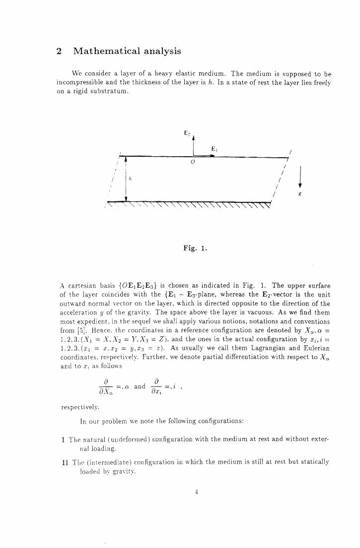
2 Mathematical analysis

We consider a layer of a heavy elastic medium. The medium is supposed to be incompressible and the thickness of the layer is h. In a state of rest the layer lies freely on a rigid substratum.

E, -! EI / n

0 7 /

1 /

/ /

/ g

Fig. 1.

A cartesian basis {OE) E 2 E3 } is chosen as indicated in Fig. 1. The upper surface of the layer coincides with the {E) - E3-plane, whereas the E 2-vector is the unit

outward normal vector on the layer. which is directed opposite to the direction of the accelerat ion 9 of the gravity. The space above the layer is vacuous. As we find them

most expedient, in the sequel we shall apply various notions, notations and conventions from [.)]. Hence. the coordinates in a reference configuration are denoted by X c> ' Q = 1, 2,3. (X) = X,X2 = Y,X3 = Z ), and the ones in the actual configuration by xi,i = 1.2.3. ( .1'1= I . .1'2 = y,x3 = z). As usually we call them Lagrangian and Eulerian coordinates . respectively. Further. we denote partial differentiation with respect to Xc> ami to X, as foUows

a --= 0 aXa .

respectively.

a and -.-= , l , ax i

In our problem we note the following configurations:

I The natural (undeformed) configuration with the medium at rest and without exter­

nal loading.

II TIle' (intermediate) configuration in which the medium is still at rest but statically

load ed by gra\'ity.

III The final configuration, which is a kinematically perturbed situation in which the medium is in motion after having received an initial disturbance from an external agency.

Since there is no essential geometric difference between I and II, we may choose the latter as the reference configuration. Hence, h is the thickness of the layer in the state II. The equations referring to the final or current state III will now be linearized with respect to state II (the small parameter being the displacement]! = ,;r - X). In II the first Piola-Kirchhoff stress tensor T, is

T, = PrgY1 , (0 ::; Y ::; h), (2.1 )

where pr is the density and 1 is the unit tensor. This stress satisfies the equilibrium equation.

(2.2)

in which Div denotes the divergence with respect to the Lagrangian coordinates x'c", together with the two pertinent boundary conditions at the free upper surface of the layer

TT12 = Trn = 0, for Y = 0, (2.3)

where the components Trio of T, refer to the cartesian basis.

In what follows we denote the Cauchy stress tensor in configuration III by T, and its components by T;j, again with respect to the (common) cartesian basis. The displacement vector 1!: occurring at the transition from II to III, together with all its derivatives with respect to Xa and Xi, is assumed to be infinitesimal by small, i.e. Ilu;,all = £ ~ 1. Hence, in 0(£) approximation we may equate the referential and spatial gradients of ]!,

Grad]! = grad1!:, (2.4 )

and, apparently, also the two divergences of ]!,

Div]! = div]!. (2.5)

In view of the incompressibility of the medium we have

(2.6.1 )

and

J = d£tF = 1, (2.6.2)

5

where :F = I + Grad.u denotes the deformation gradient. Hence, from the relation

(2.7)

and observing that T,. and T are of 0(1), it follows that in O(f) approximation

T,. = T(I - grad.uf, (2.8.1 )

or, in components,

(2.8.2)

For.u = Q, the Cauchy stress tensor T is equal to T,. in II according to (2.1), as is to be expected. In view of this, the following (linearized) constitutive relation is obvious

(2 .9)

where p is the increase of the pressure, [ is the linearized strain tensor defined as ~(grad.J! + (grad.J!)T), and p is the shear modulus. We note that pip and [ are O(f). Then from (2.8) we find in O(f) approximation

T,. = PrqYI - pI + 2J1[ - PrgY(grad.uf, (2.10.1)

or , in components ,

(2.10.2)

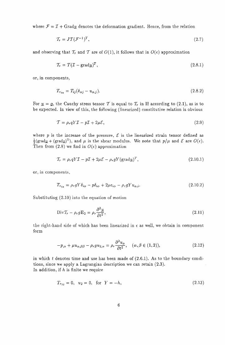
Substituting (2.10) into the equation of motion

(2.11)

the right-hand side of which has been linearized in f as well, we obtain in component form

(2.12)

in which t denotes time and use has been made of (2.6.1). As to the boundary condi­tions, since we apply a Lagrangian description we can retain (2.3). In addition , if h is finite we require

TT12 = 0, U2 = 0, for Y = -h, (2.13)

6

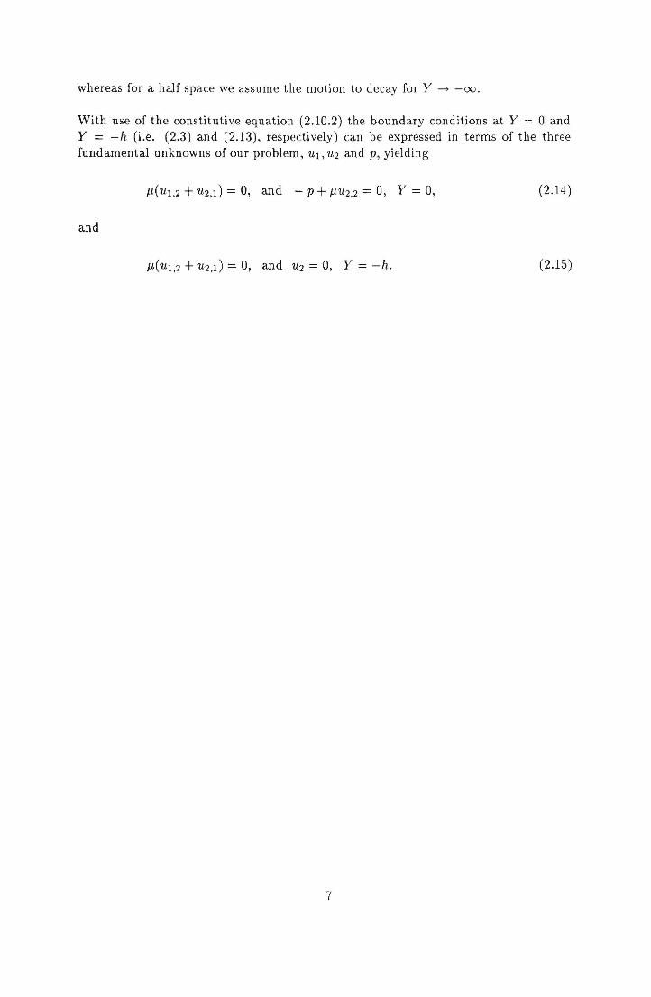
whereas for a half space we assume the motion to decay for Y ----. -00.

With use of the constitutive equation (2.10 .2) the boundary conditions at Y = ° and Y = -h (i.e. (2.3) and (2.13), respectively) can be expressed in terms of the three fundamental unknowns of our problem, Ul, U2 and p, yielding

J.L(Ul.2 + u2.d = 0, and - p + J.LU2.2 = 0, Y = 0, (2.14)

and

(2.15)

7

3 Surface waves

In this section we shall calculate the velocity of propagation of two-dimensional surface waves of the type

(3.1 )

Applying the decomposition theorem of Helmholtz we write (cL [2])

(3.2)

where <f; and 'lj; are functions of X, Y and t. From (2.6.1) it follows that in O(E) approximation

b.<f; = 0 , (3.3)

where b. denotes the two-dimensional Laplace operator. Moreoyer, substitution from (3.2) into (2.12) yields

ap a a ( a¢ a'lj; ) a2

(o¢ o'lj; ) - aX + J-l aY (6'lj;) - Prg aX ay - aX = Pr at2 aX + aY ,(3.4.1)

and

These two equations will be satisfied jf

(3.5.1)

(C2 is the velocity of shear waves) and

( a¢ av' ) 02¢

-p - Prg oY - ax = Pr ot2 + C , (3.5.2)

where the constant C may be equated to zero without impairing the generality of the solution considered. The Laplace equation (3.3) and the wave equation (3.5.1) form the basic equations of our problem; the relation (3.5.2) will be used to eliminate the pressure p from the boundary conditions (2.14). Thus, the boundary conditions (2.14) and (2.15) become (with use of (3.2))

(3.6)

8

for Y = 0, and

fJ¢ fJ'Ij; fJY - fJX = 0 ,

fJ2 ¢ fJ2'1j; fJ2'1j; 2 fJXfJY + fJy2 - fJX2 = 0 , (3.7)

for Y = -h. Through the use of (3.5.1) we can simplify (3.7) into

fJ¢ fJy = 0, and 'Ij; = 0, for Y = -h , (3.8)

without impairing the generality of the solution.

Let us now consider a sinusoidal wave of frequency pI27r, propagating in the E l -

direction with velocity c and wavelength 27r I f, so that c = pi f. Then we may try as solutions of (3.3) and (3.5.1)

¢ = F(Y)ei(pt-fX) , 'Ij; = G(Y)ei(pt-fX).

In the usual way it appears that

¢ = (AI cosh fY + A2 sinh fY)ei(pt-fX) ,

'Ij; = (Bl sinh sY + B2 cosh sY)ei(pt-fX) ,

(3.9)

(3.10.1)

(3.10.2)

where s2 = P - (pi C2)2. The constants AI, A2, Bl and B2 are to be determined from the boundary conditions (3.6) and (3.8). We thus find

- f Al sinh fh + f A2 cosh fh = 0 ,

-Bl sinh sh + B2 cosh sh = 0 . (3.11)

In what follows we shall make use of the following dimensionless quantities

SI = ~, kl = ..!:.., j = fh, g = Prg , f C2 I1f

(3.12)

so that sh = Slj, and si = 1 - ki- Apparently, if k1 ::; 1, then Sl is real; otherwise it is an imaginary number.

9

In order to obtain from (3 .11) a non-trivial solution the determin ant of the coef­ficients of AI , A 2, B1 , B2 must be zero. From this we find the following relation for the dimensionless gravity constant !J as a function of the normalized wave velocity kl and the dimensionless wave number j, (valid for kl f 0 and kl f 1)

" -4.)1 - ki tanh j + (2 - kf)2 tanh(}.)l - kf) !J = G( kl' J) = " "

kf tanh f tanh (f .) 1 - kf) (3.13)

10

. I j .

10 -

, ~ - !

4 Discussion

Evidently, the normalized gravity constant g cannot be negative. This restricts the domain of the function (3.13). In the further discussion we shall consider the cases o < k1 < 1, and kl > 1 separately.

Case 0 < kl < 1

We see that in this case all terms occurring on the right-hand side of (3.13) are real . Moreover, if h -. 00, Le. j -. 00, then

( 4.1)

Apparently, 9 = 0 then corresponds with

(4.2)

By inspection we see that this equation agrees with the corresponding one for Rayleigh waves through an elastic half space as obtained by Kolsky [5) , if his result is applied to an incompressible medium (Le. 01 = 0 in his expression (2.37)).

We note that (4 .1) yields positive values of 9 if (for kl E (0 , 1))

0.9553 < kl < 1.

I

I 0.51

I I

I

(4.3)

j ~oo

j= 10

/=7

°Li ______________ ~~I ------------~---\

o ~ ______________ ~~ __ ~~ ____ ~~ 0.9 0.95 \ 1.0 k I 0.9

~ 'l"

Fig. 2.

11

For finite values of j this domain shrinks with decreasing j. Our numerical re­

sults. which are visualized in Fig. 2.a, reveal that there ex.ists a lower limit jo(kd for

r 1.:1 E (0.9.553 , 1), below which no positive solutions for 9 can be obtained from (3.13). Investigation of the behaviour of G(k1 , j) in the neighbourhood of kl = 1 shows

that a necessary condition for G > 0 is j > 4 tanh j, which is satisfied if j > 4.

Figure 2.b shows the dimensionless gravity constant g, calculated according to (3.13), as a function of the dimensionless veloci ty of propagation kl for several values of the dimensionless wave number j, including j -+ 00. The domain of this function is here restricted to k) < 1.

Case k) > 1

In this case we have to replace R by iJk? - 1, but the right-hand side of

(3.13) remains real. For jJq - 1 :f. m!'. n E IN, we rewrite (3.13) in the fonn

. _ 4~ (2_q)2 9 = G( 1.:). j) = - _ ~ + 2 - .

qtan(fVJ.:f - 1) k)tanhf ( 4.-1 )

\\'e see that for fixed kl and increasing depth h, i.e. growing f, the denominator of the first terlll Oil the right-hand side of (-1.4) goes to zero whenever

j~-n7r .nE}.\;. (4.5 )

Apparently. 9 continuously changes sign. and we infer that not every combination of k) and j is possible (i.e. yields positive values for fJ). On the other hand, if we consider

!J as a fUIlction of 1..-1 for a fixed value of j. it appears that the intervals in which the

first term dominates owr the second one. and thus may render negative values of g. ~hrillk with illcreasing 1..- 1, Outside the immediate neighbourhood of the above singular

points. and for sll fhciently large I..- J • the value of 9 follows from the second term on the

righl-hand sidf' of (-l.-l) \\it h sufficient accuracy. For large kJ this yields

k2 - 1 !J::::;~--.

tanhf

which agrees with the well-known formula

c = gtanh(jh )

f

for water waws [-1 ].

12

(4.6 )

(4.7)

I- - - - - - - - - - - - - - - - - - - - - - - - - - - - - - - - - -- --

------

0.5

r - - - - - - - - - - - - - - -- - - - - - - - - - - - - - - - - - - - - - - --

I ~ -----0 ~~ /

~ '~ I

2 g

51

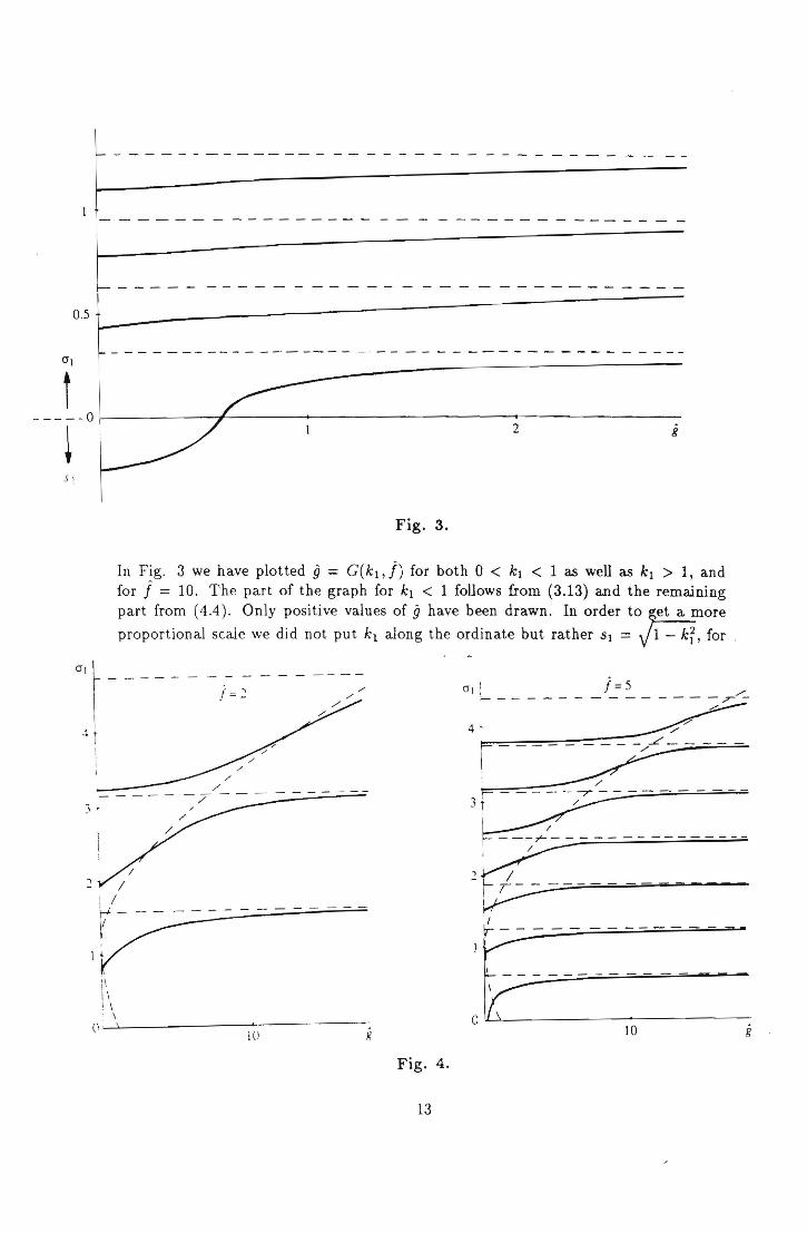
Fig. 3.

In Fig. 3 we have plot ted 9 = G( k1' j) for both 0 < k1 < 1 as well as k1 > 1, and for j = 10. The part of the graph for k1 < 1 follows from (3 _13) and the remaining part from (4.4). Only positive values of 9 have been drawn. In order to ~more

proportional scale we did not put k1 along the ordinate but rather Sl = VI - kr, for

3 •

I

2 / I /

f;;-:-­lV

1\ 1\ I \

\

f ='2 /' /'

() ~ . ...1-______ -'-_____ --:

10 g

Fig. 4.

13

( 1 ) j=5 /' ~--------------T-

4" ~ ...L r ~~~~~

P:::: - -r-

3~ ____ n __ _

, I~ ~~~--------=--------­

/

10

kl < 1 and 0'1 = Jk? - 1, for kl > 1. From the figure we see that for each value of 9 an infinite set of k1-values can be found , but almost all of these values are larger than one. Only for 0 < 9 < 0.6 (in the case f = 10) one value for kl < 1 can be obtained.

In case kl < 1 the number S occuring in the solution for 1/J according to (3.10.2) is real, implying that in the case of a half space (h ~ (0) this function decays ex­ponentially for Y ...... -00. Hence, in this case we deal with a surface wave. On the other hand , if kl > 1, the coefficient s becomes a purely imaginary number and then 'l/J becomes periodic in Y. So, the case kl > 1 does not lead to surface waves, even not in the case of a half space. From this we conclude that, in case j = 10, surface waves only occur if 9 E (0,0.6) (a result which can also be read off from Fig. 2.b).

Finally, ill Fig. 4 two graphs are given , showing 9 = G(kl' j) according to (4.4)

as a function of 0'1 = Jq - 1. for kl > 1, and for j = 2 and j = 5, respectively. The dotted line in these graphs represents the second term on the right-hand side of (4.4) . For larger val ues of 0'1 and away from the singular points given by (4 .5) we see that the g-curves and the dotted line approach each other. This becomes even more clear in Fig . . 5 .. where for j = 2 the analoug graph is drawn but now for larger values of g and 0'1 . (up to 9 = 130 and 0'1 E [3 . 11 J, respecti\"ely.

~­I O ~

~--~~~~==-'-=:::/ - - - - - - - -

s

o

'1 y-

10 50

Fig. 5.

14

- -I

100

Figure captions

Fig. 1. The layer resting on a rigid foundation

Fig. 2.a. The lower limit jo(kd for j(k~O) = 0.955)

Fig. 2.h. 9 as a function of k1 (for k1 < 1) with j as parameter.

Fig. 3. 9 as a function of 81 = VI - kr, for k1 < 1, and of 0"1 - jk'i, for k1 > 1, with

j = 10.

Fig. 4. 9 as a function of 0"1 = jk'i, kr, for j = 2 and j = 5.

Fig. 5. g-curves for higher values of 9 and 0"1; comparison with last term of (4.4) (dotted line)

References

1. K.F. Graff, Wave motion in elastic solids, Clarendon Press, Oxford (1975).

2. H. Kolsky, Stress waves in solids, Clarendon Press, Oxford (1953).

3. H. Lamb, Hydrodynamics, University Pr('ss, Cambridge (1962).

4. J.J. Stoker, Water waves, Interscience Publishers, Inc., New York (1957).

5. C. Truesdell and W. Noll, The non-linear field theories of mechanics, Encyclopedia of physics, Vol. III/3, Springer Verlag, Berlin (1965).

6. E. Trefftz, Zur Theorie der Stabilitat des elastischen Gleichgewichts, Zeitschr. f. angew. Math. und Mech., 13, 160-165, 1933.

7. C.E. Pearson, Theoretical elasticity, Harvard University Press, Cambridge, Mas­sachusetts (1959).

8. A.E. Green and J .E. Adkins, Large elastic deformations, Clarendon Press, Oxford (1960).

9. S. Timoshenko and J .M. Gere, Theory of elastic stability, McGraw-Hill Book Co., New York (1961).