Ray Tracing Tutorialby the Codermind team

Contents:

1. Introduction : What is ray tracing ?

2. Part I : First rays

3. Part II : Phong, Blinn, supersampling, sRGB and exposure

4. Part III : Procedural textures, bump mapping, cube environment map

5. Part IV : Depth of field, Fresnel, blobs

2

This article is the foreword of a serie of article about ray tracing. It's probably a word that you may have heard without really knowing what it represents or without an idea of how to implement one using a programming language. This article and the following will try to fill that for you. Note that this introduction is covering generalities about ray tracing and will not enter into much details of our implementation. If you're interested about actual implementation, formulas and code please skip this and go to part one after this introduction.

What is ray tracing ?

Ray tracing is one of the numerous techniques that exist to render images with computers. The idea behind ray tracing is that physically correct images are composed by light and that light will usually come from a light source and bounce around as light rays (following a broken line path) in a scene before hitting our eyes or a camera. By being able to reproduce in computer simulation the path followed from a light source to our eye we would then be able to determine what our eye sees.

Of course it's not as simple as it sounds. We need some method to follow these rays as the nature has an infinite amount of computation available but we have not. One of the most natural idea of ray tracing is that we only care about the rays that hit our eyes directly or after a few rebounds. The second idea is that our generated images will usually be grids of pixels with a limited resolution. Those two ideas together form the basis of most basic raytracers. We will place our point of view in a 3D scene, and we will shoot rays exclusively from this point of view and towards a representation of our 2D grid in space. We will then try to evaluate the amount of rebounds needed to go from the light source to our eye. This is mostly okay because the actual light simulation does not take into account the actual direction of the ray to be accurate. Of course it is a simplification we'll see later why.

How are raytracers used ?

The ideas behind ray tracing (in its most basic form) are so simple, we would at first like to use it everywhere. But it's not used everywhere.

Ray tracing has been used in production environment for off-line rendering for a few decades now. That is rendering that doesn't need to have finished the whole scene in less than a few milliseconds. Of course we should not generalize and let you know that several implementations of raytracer have been able to hit the "interactive" mark. Right now so called "real-time ray tracing" is a very active field right now, as it's been seen as the next big thing that 3D

3

accelerators need to be accelerating. Raytracer are really liked in areas where the quality of reflections is important. A lot of effects that seem hard to achieve with other techniques are very natural using a raytracer. Reflection, refraction, depth of field, high quality shadows. Of course that doesn't necessarily mean they are fast.

Graphics card on the other hand they generate the majority of images these days but are very limited at ray tracing. Nobody can say if that limitation will be removed in the future but it is a strong one today. The alternative to ray tracing that graphics card use is rasterization. Rasterization has a different view on image generation. Its primitive is not rays, but it is triangles. For each triangle in the scene you would estimate its coverage on the screen and then for each visible pixel that is touched by a triangle you would compute its actual color. Graphics cards are very good at rasterization because they can do a lot of optimization related to this. Each triangle is drawn independently from the precedent in what we call an "immediate mode". This immediate mode knows only what the triangle is made of, and compute its color based on a serie of attributes like shader program, global constants, interpolated attributes, textures. A rasterizer would for example typically draw reflection using an intermediate pass called render to texture, a previous rasterizer pass would feed into itself, but with the same original limitations which then cause all kind of precision issues. This amnesia and several other optimizations are what allow the triangle drawing to be fast. Raytracing on the other hand doesn't forget about the whole geometry of the scene after the ray is launched. In fact it doesn't necessarily know in advance what triangles, or objects it will hit, and because of interreflexion they may not be constrained to a single portion of space. Ray tracing tends to be "global", rasterization tends to be "local". There is no branching besides simple decisions in rasterization, branching is everywhere on ray tracing.

Ray tracing is not used everywhere in off line rendering either. The speed advantage of rasterization and other techniques (scan line rendering, mesh subdivision and fast rendering of micro facets) has often been hold against true "ray tracing solution", especially for primary rays. Primary rays are the one that hit the eye directly, instead of having rebound. Those primary rays are coherent and they can be accelerated with projective math (the attribute interpolation that fast rasterizers rely upon). For secondary ray (after a surface has been reflecting it, or refracting it), all bets are off because those nice properties disappear.

In the interest of full disclosure it should be noted that ray tracing maths can be used to generate data for rasterizer for example. Global illumination simulation may need to shoot ray to determine local properties such as ambiant occlusion or light bleeding. As long as the data is made local in the process that will be able to help a strict "immediate renderer".

Complications, infinity and recursion

Raytracers cannot and will not be a complete solution. No solution exist that can deal with true random infinity. It's often a trade off, trying to concentrate on what makes or break an image and its apparent realism. Even for off line renderer performance is important. It's hard to decide to shoot billions of rays per millions of pixel. Even if that's what the simulation seems to require. What trade offs do we need to do ? We need to decide to not follow every path possible.

Global illumination is a good example. In global illumination techniques such as photon mapping, we try to shorten the path between the light and the surface we're on. In all generality, doing full global illumination would require to cast infinite amount of ray in all the directions and see which percentage hit the light. We can do that but it's going to be very slow, instead, we'll first cast photons (using the exact same algorithm as ray tracing but in reverse from the light point of view) and see what surface they hit. Then we use that information to compute lighting in first approximation at each surface point. We only follow a new ray if we can have a good idea using a couple of rays (perfect reflection needs only one additional ray). Even then it can be expensive, as the tree of rays expands at a geometric rate. We have often to limit ourself to a maximum depth recursion.

Acceleration structure.

Even then, we'll want to go faster. Making intersection tests becomes the bottleneck if we have thousand or millions of intersectable objects in the scene and go for a linear search of intersection for each ray. Instead we definitely need an acceleration structure. Often used are hierarchical representation of a scene. Something like a KD-Tree or octree would come to mind. The structure

4

that we'll use may depend on the type of scene that we intend to render, or the constraints such as "it needs to be updated for dynamic objects", or "we can't address more than that amount of memory", etc. Acceleration structures can also hold photons for the photon mapping, and various other things (collisions for physics).

We can also exploit the coherence of primary rays. Some people will go as far as implementing two solutions, one that use rasterization or similar technique for primary rays and raytracing for anything beyond that. We of course need a good mean of communication between both stages and a hardware that is sufficiently competent at both.

«First RAYS»

This is the first part of the ray tracing series of tutorials. We've seen in the introduction what a raytracer was and how it was different from other solutions. Now let's concentrate on what it would requires to implement one in C/C++.

Our raytracer will have the following functionality. It will not try to be real time, and so will not take shortcuts because of performance only. Its code will try to stay as straightforward as possible, that means we'll try not to introduce complex algorithms. If we can avoid it. We'll make sure the basic concepts explained here will be visible in the code itself. The raytracer will work as a command line executable, that will take a scene file such as this one and output an image such as this one :

What does the raytracer do ?

First start with a simple pseudo language description of the basic ray tracing algorithm.

for each pixel of the screen{ Final color = 0; Ray = { starting point, direction }; Repeat {

5

for each object in the scene { determine closest ray object/intersection; } if intersection exists { for each light in the scene { if the light is not in shadow of another object { add this light contribution to computed color; } } } Final color = Final color + computed color * previous reflection factor; reflection factor = reflection factor * surface reflection property; increment depth; } until reflection factor is 0 or maximum depth is reached;} For this first part, we'll limit ourselves to spheres as objects (a center point and a radius), and point lights as light sources (a center point and an intensity).

Scanning the screen

We have to cast a ray, at each one of our pixel to determine its color. This translates as the following C code :

for (int y = 0; y < myScene.sizey; ++y) { for (int x = 0; x < myScene.sizex; ++x) { // ... } }Well so far no difficulty. Once we computed the final color we'll simply write it to our TGA file as this :

imageFile.put(min(blue*255.0f,255.0f)). put(min(green*255.0f, 255.0f)). put(min(red*255.0f, 255.0f));Okay, a few comments on this. First it should be noted that all the colors inside our code will be treated as three components floating point numbers. We'll see the importance of that later. But the TGA file itself is storing its data using a fixed precision 8 bits per component color. So we'll need to do a conversion. In this first page, a naive "saturation operator", that is clamp any value above 1.0f, then convert the result into an integer number between 0 and 255. We'll also see later why the clamping is considered "naive". Please bear with us in the meantime.

Now casting rays for good

We've got our starting point. It's somewhere on our projection screen. We arbitrarily decide to make all our rays point in a single direction (towards the positive Z coordinate).

ray viewRay = { {float(x), float(y), -1000.0f}, { 0.0f, 0.0f, 1.0f}};The single direction is important because it defines our projection. Every ray will be perpendicular to the screen, that means that we'll do the equivalent of splatting our scene along parallel lines toward the screen. It's called perpendicular projection (also known as orthographic projection). There are other types of projection (conic projection being another big one, and we'll introduce it later).

6

Types of projection change the way the ray are related to each other. But it should be noted that it doesn't change anything to the behavior of a single ray. So you'll see that even later when we change our code to handle conic perspective, the rest of the code, intersection and lighting will NOT change the least bit. That's a nice property of raytracing compared to other methods, for example rasterization hardware relies heavily on the property of orthographic/conic perspective.

We set the starting point at an arbitrary position that we hope will enclose the whole visible scene. Ideally there should be no clipping, so the starting point will depend on the scene. But it should not be too far, as too big a floating point number will cause floating point precision errors in the rendering.

When we'll go "conic", such a problem of determination of the starting point will disappear because the positions behind the oberver are then ILLEGAL.

The closest intersection

The ray is defined by its starting point and its direction (normalized) and is then parameterized by a arithmetic distance called "t". It denotes the distance from any point of the ray to the starting point of the ray.

We only move in one direction on the ray from the smaller t to the bigger t. We'll iterate through each object, determine if there is an intersection point, we'll find the corresponding t parameter of this intersection and we'll find the closest one by taking the smallest t that is positive (that means it's in front of our starting point not behind).

Sphere-Ray intersection

Since we're only dealing with spheres our code only contains a sphere-ray intersection function. It is one of the fastest and simplest intersection code that exists. That's why we start with spheres here. The math themselves are not that interesting we'll introduce our parameter inside an intersection equation. That will give us a second degree equation with one unknown t.

7

We compute the delta of the equation and if the delta is less than zero there is no solution, so no intersection and if it's greater than zero there is at most two solutions. We take the closest one. If you want more details to how we got to this please consult our Answers section (What is the intersection of a ray and a sphere ?). Here is the code of that function :

vecteur dist = s.pos - r.start; double B = r.dir * dist; double D = B*B - dist * dist + s.size * s.size; if (D < 0.0f) return false; double t0 = B - sqrt(D); double t1 = B + sqrt(D); bool retvalue = false; if ((t0 > 0.1f) && (t0 < t)) { t = (float)t0; retvalue = true; } if ((t1 > 0.1f) && (t1 < t)) { t = (float)t1; retvalue = true; }We take the closest one, but it has to be further than the starting point, that is why we compare t0 and t1 to 0.1f. Why not 0.0f ? Simply because there is a high risk that given our limited precision (in float), that after a reflection from a point we find that our ray, intersects the same object around the same point when it shouldn't with an infinite precision. By taking our starting point at a reasonable distance but close enough to not cause "gaps" we can avoid some artifacts.

Lighting our intersection point

The lighting in one point is equal to the sum of the contribution of each individual light source. The problem here is way oversimplified by providing a finite list of well defined point lights.

We rapidly cull any light that is not visible from our side of the surface. That is if the exiting normal to our sphere and the light direction, point towards opposite direction. This is achieved by this simple code :

// sign of dot product tells if they're pointing in the same direction if ( n * dist <= 0.0f ) continue;Then we determine if the point is in the shadow of another object for this particular light.

The code for this is similar to the intersection code that we had previously. We will cast a ray from our intersection point towards the light source (it's possible because it is a point light, that is a single point in space). But this time we don't care to find what the ray is intersecting or at what

8

distance. As soon as we find an intersection point between this new ray and any object in the scene we stop the iteration because we know that the object is in the light shadow.

Lambert

Lambert was a European mathematician of the 18th century. Lambert cosine's law is a relation between the angle an incoming light ray has with a surface, the light intensity of this ray and the amount of light energy that is received by unit of surface. In short if the angle is low (grazing light), the received energy is low, and if the angle is high (zenith) the energy is high. That law will for example in an unrelated topic explain why the temperature at the equator is higher than the temperature at the earth poles.

How is that important to us ? If we are given a perfectly diffusing surface, that's the only thing that will matter to compute the lighting. The property of diffusion is that the energy that is received in one direction is absorbed and partially reemitted in all directions. A perfect diffuse surface will emit the same amount of energy in all directions. That important property is why the perceived lighting of a surface that is perfectly diffuse will only depend on the angle of the incident light with that surface : it is totally independent of the viewing angle. Such a material is also called a lambertian, because its lighting property is only determined by the lambert's law described above (that's the only type of material that we support in this first chapter. For more complex models see the following chapters). On the illustration below, you can see the incoming light and the redistributed energy, it is constant in all direction that's why it's represented in a perfect circle.

When we hit such a surface in our raytracer code, we will compute the cosine of the angle theta that the incoming ray does with the surface (via the normal) :

float lambert = (lightRay.dir * n) * coef;Then we multiply that lambertian coeficient with the diffuse color property of the surface, that will give us the perceived lighting for the current viewing ray.

Reflection

What would be ray tracing without that good old perfect (though irrealist) reflection. In addition to the diffusion color attribute described above, we'll give our surface a reflection coefficient. If this coefficient is 0, then that surface is not reflective at all and we can stop our iteration for this pixel and go to the next one. If this coefficient is greater than 0, then part of the lighting for that surface will be computed by launching a new ray from a new starting point at the incident point on that surface. The direction of the new ray, is the "reflected" direction, reflection of the incident view ray by the surface normal.

float reflet = 2.0f * (viewRay.dir * n); viewRay.start = newStart; viewRay.dir = viewRay.dir - reflet * n; We could potentially end up in a situation where each new ray would hit a surface and be reflected and so on forever. In order to avoid infinite loop, we arbitrarily limit the number of

9

iterations by pixel (for example, no more than ten iterations in the current code). Of course when we hit that limitation the lighting will be wrong, but as long as we have no perfect reflection (less than a hundred percent) each iteration will contribute less than the previous one to the overall lighting. So hopefully cutting after the tenth iteration will not cause too many visual issues. We could alter that if we are to render a special scene that still requires more (a hall of mirror type of scene for example).

Digression : Computing successive reflections seems to be a natural fit for an recursive algorithm "from the book", but in practice and in our case, we preferred to go for an iterative algorithm. We save on the C stack usage but it will also require us to do some trade off in flexibility later.

The lighting models that we use here (Lambert + perfect reflection) are way too limited to render the complex natural materials. Other types of models (Phong, Blinn, Anisotropic, BRDF theory...) need to be introduced to account for more. We'll come back to it later.

As we saw previously in our first part, a perfectly diffuse material will send incident light back uniformly in all directions. At the other side of the spectrum, a perfect mirror only sends light in the opposite direction of the incident ray.

Reality is not as black and white as that, real object surfaces are often complex and difficult to model simply. I will describe here two empirical models of "shiny" surfaces that are not pure mirror.

This is the second part of the our series of articles about ray tracing in C++. It follows the part called "First rays".

Phong

Bui Tuong Phong was a student at the University of Utah when he invented the process that took his name (Phong lighting). It is a quick and dirty way to render objects that reflect light in a priviledged direction without a full blown reflection. In most cases that priviledged direction is that of the light vector, reflected by the normal vector of the surface.

The common usage is to describe that as the specular term, opposed to the diffuse term from the Lambert formula. The specular term varies based on the position of the observer, as you can see below in the equation that takes into account viewRay.dir :

float reflet = 2.0f * (lightRay.dir * n); vecteur phongDir = lightRay.dir - reflet * n; float phongTerm = _MAX(phongDir * viewRay.dir, 0.0f) ; phongTerm = currentMat.specvalue * powf(phongTerm, currentMat.specpower) * coef; red += phongTerm * current.red; green += phongTerm * current.green; blue += phongTerm * current.blue;Here is the result of the previous scene with some added Phong specular term:

10

Digression: an amusing story about the Phong lighting is that in papers that Bui Tuong Phong wrote his name is written in this order, which is the traditional order in Vietnam (and sometimes also in other countries where the given name is quoted after the family name). But for most english speaking readers that order is reversed and so people assumed his last name was Phong. Otherwise his work would have been known as the Bui Tuong lighting.

Blinn-Phong

A possible variation on the specular term is the derived version based on the work of Jim Blinn, who was at the time professor for Bui Tuong Phong in Salt Lake City and is now working for Microsoft Research.

Jim Blinn added some physical considerations to the initial empiric result. This goes through the computation of an intermediate vector at the midpoint between the light direction and the viewer's one (Blinn's vector). Then it goes through the computation of the dot product of this Blinn vector with the normal to the surface. A comparison with previous formula allows us to see that Blinn term is equally maximum when the view ray is the reflected of the light ray : it is a specular term.

vecteur blinnDir = lightRay.dir - viewRay.dir; float temp = sqrtf( blinnDir * blinnDir); if (temp != 0.0f ) { blinnDir = (1.0f / temp) * blinnDir; float blinnTerm = _MAX(blinnDir * n, 0.0f); blinnTerm = currentMat.specvalue * powf(blinnTerm , currentMat.specpower) * coef; red += blinnTerm * current.red ; green += blinnTerm * current.green ; blue += blinnTerm * current.blue; }Here is the result of the Blinn-Phong version. As you can see the output is pretty similar, this is the version we will use for the remaining of the series.

11

Antialiasing

There are numerous methods aimed at reducing aliasing. This article is not meant to be a complete description of what anti-aliasing does, or a complete directory of all the methods. For now we'll just describe our current solution which is based on basic supersampling.

The supersampling is the idea that you can take more individual color samples per pixel in order to reduce aliasing problems (mostly stair effect and to some extent moire effect). In our case for a final image of X,Y resolution, we'll render to the higher resolution of 2*X, 2*Y then take the average of four samples to get the color of one pixel. This is effectively a 4x supersampling because we're computing four times more rays per pixels. This is not necessary that those four extra samples are within the boundary of the original pixel, or that the averaging be a regular arithmetic average. But more on that later.

You can see on the following code how it goes. For each pixel that we have to compute we will effectively launch four rays, but those rays will see their contribution reduced to the quarter. The relative position of each pixel is free. But for simplicity reason and for now we'll just order them on a regular grid (as if we had just computed a four times larger image).

for (int y = 0; y < myScene.sizey; ++y) for (int x = 0; x < myScene.sizex; ++x) { float red = 0, green = 0, blue = 0; for(float fragmentx = x; fragmentx < x + 1.0f; fragmentx += 0.5f) for(float fragmenty = y; fragmenty < y + 1.0f; fragmenty += 0.5f) { // Each ray contribute to the quarter of a full pixel contribution. float coef = 0.25f; // Then just launch rays as we did before } // Then the contribution of each ray is added and the result is put into the image file } Here is the result of the applied 4x supersampling, greatly zoomed in:

12

Gamma function

Originally CRTs didn't have good restitution curve. That is the relation between a color stored in a frame buffer and its perceived intensity on the screen would not be "linear". Usually you would instead have something like Iscreen = Pow(I, gamma), with gamma greater than 1.

In order to correctly reproduce linear gradients or anything that rely on the good linear relation (for example dithering and anti-aliasing), you would then have to take into account this function when doing all your computations. In the case above for example, you would have to apply the inverse function Pow(I, 1/gamma). Nowadays that correction can be done at any point in the visualization pipeline, modern PC have even dedicated hardware in their DAC (digital to analog converter) that can apply this inverse function to the color stored into the frame buffer just before sending it to the monitor. But that's not the whole story.

To provide a file format that would be calibrated in advance for all kind of configurations (monitors, applications, graphics cards) that could exist out there is the squaring of the circle : it's impossible. Instead we rely on conventions and explicit tables (the jpeg format has profiles that describe what kind of response the monitor should provide to the encoded colors, then the application layer can match that to the profile provided for the monitor). For the world wide web and Windows platforms a standard has been defined, it is called sRGB. Any file or buffer that is sRGB encoded has had its color multiplied by the power of 1/2.2 before being written out to the file. In our raytracer we deal with a 32 bit float per color component, we have a lot of extra precision, that way we can apply the sRGB transform just before downconverting to 8 bit integer per component.

Here is an image that is sRGB encoded. Your monitor should have been calibrated to minimize the perceived difference between the solid gray parts and the dithered black and white pattern. (It will be harder to calibrate your LCD than your CRT, because, on typical LCDs, angle of view will impact the perceived relation between intensities but you should be able to find a spot that is good enough hopefully).

What would be the interest to encode images in sRGB format, rather than have them encoded in a linear color space and let the application/graphics card apply the necessary corrections at the end ? Well other than the fact that it is the standard and having your png or tga file in an sRGB space will ensure that the viewer if he's correctly calibrated will see them as you would expect, sRGB can be seen as a form of compression also. The human eye is more sensitive to lower intensity and so when reducing the 32 bit color to a 8 bit value you have less risk of having visible

13

banding when reproducing them. Because the pow(1/2.2) transform gives more precision to the lower intensity. (of course that's a poor compression, anything other than TGA is better, like jpeg or png, but since we output a tga file, the loss are already "factored in").

Here is the corresponding code :

float srgbEncode(float c){ if (c <= 0.0031308f) { return 12.92f * c; } else { return 1.055f * powf(c, 0.4166667f) - 0.055f; // Inverse gamma 2.4 }}//.. // gamma correction output.blue = srgbEncode(output.blue); output.red = srgbEncode(output.red); output.green = srgbEncode(output.green);

Photo exposure

On the previous page, I talked about the fact that the use of the min function in our float conversion to int was a "naive" approach. Let me detail that. We call that operator a saturation operator. What is saturation ? This term has a lot of different usage, you can encounter it in electronics, music, photography, etc. What it means in this case is that a signal that varies on a large interval is going to be converted to a smaller interval but with everything that was bigger than the max value of that smaller interval will be set equal to the max value itself. With this approach on the following diagram, any value that was between 1 and 2 will be seen as 1.

This works well only if all the interesting values are below 1. But in reality and in image synthesis this is not the case. Intensity in an image can vary wildly. The closer an object goes to a light source the brighter it becomes and this brightness is not limited artificially. Also ideally, we would like to have details in the high intensity as well as the low intensity. This approach is called tone mapping (mapping higher range values to a lower range value without losing too much details).

Photo exposure is one possible tone mapping operator. In real life photography with film, we used to have chemical surface where a component would migrate from one form to another as long as light would come on it. And the speed of migration would be dependant on the intensity of the light (flow of photons). After their migration they would become inert, slowing down the rate of migration over time. Areas with a lot of migration would appear brighter (after the intermediate use of a negative film or not) and those without migration would appear darker. With an infinite exposure time, all component would have migrated. Of course this is a gross simplification of the whole process, but this can give us an idea of how to deal with possibly unbound intensity. Our exposure function takes the final intensity as an exponential function of exposure time and light linear intensity. 1 - exp(lambda * I * duration).

14

Here is the corresponding code :

float exposure = -1.00f; blue = 1.0f - expf(blue * exposure); red = 1.0f - expf(red * exposure); green = 1.0f - expf(green * exposure); "Exposure" is a simplified term, no need to carry all the real life implications (at least in the scope of this limited tutorial).

The first image below, uses the original "saturation" operator and as we submit it to a bright light suffers from serious saturation artefacts. The second image uses our exposure operator and we submit it to the same light.

Digression : The exposure computation takes place before the gamme correction. We would also have to define automatically the exposure value instead of the hard coded value that we use above. Ideally an artist would select the right exposure amount until he gets what he wants from the image. Other effects such as blooming, halos, can simulate the effect of brighter lights on camera and our eye. Some bloom will happen naturally (due to foggy conditions, or because of

15

"color leaking" in the whole photography process, or because of small defects in our eyes), but most of the time they are added for dramatic effect. We won't use those in our program, but you could add those as an exercise.Here is the output of the program with the notions brought up in this page :

Now that we've seen how to treat some simple surface properties, we will try to add a few more details to our scenes. One of the simplest way to add details is via the use of textures.

I won't cover the texturing in its full exhaustive details, but I will detail here two concepts, one is the procedural texture and the other one is the environment texture or cubemap.

Specularity, supersampling, gamma correction and photo exposure

Perlin noise

Ken Perlin is one of the pionneers of the image synthesis field. He contributed to movies such as Tron, and his famous "noise" is one of the most used formula in the world of graphics. You can go and visit his webpage to learn more about his current project : http://mrl.nyu.edu/~perlin/. It's also on that website that you can find the source code for his noise algorithm that is remarkably simple. Here is the C++ version that I used and that is directly translated from the original version in java :

struct perlin{ int p[512]; perlin(void); static perlin & getInstance(){static perlin instance; returninstance;}

16

};

static intpermutation[] = { 151,160,137,91,90,15, 131,13,201,95,96,53,194,233,7,225,140,36,103,30,69,142,8,99,37,240,21,10,23, 190,6,148,247,120,234,75,0,26,197,62,94,252,219,203,117,35,11,32,57,177,33, 88,237,149,56,87,174,20,125,136,171,168,68,175,74,165,71,134,139,48,27,166, 77,146,158,231,83,111,229,122,60,211,133,230,220,105,92,41,55,46,245,40,244, 102,143,54, 65,25,63,161, 1,216,80,73,209,76,132,187,208,89,18,169,200,196, 135,130,116,188,159,86,164,100,109,198,173,186,3,64,52,217,226,250,124,123, 5,202,38,147,118,126,255,82,85,212,207,206,59,227,47,16,58,17,182,189,28,42, 23,183,170,213,119,248,152, 2,44,154,163, 70,221,153,101,155,167,43,172,9, 129,22,39,253,19,98,108,110,79,113,224,232,178,185, 112,104,218,246,97,228, 251,34,242,193,238,210,144,12,191,179,162,241,81,51,145,235,249,14,239,107, 49,192,214, 31,181,199,106,157,184, 84,204,176,115,121,50,45,127,4,150,254, 138,236,205,93,222,114,67,29,24,72,243,141,128,195,78,66,215,61,156,180};

static double fade(double t){ return t * t * t * (t * (t * 6 - 15) + 10);}

static double lerp(double t, double a, double b) { return a + t * (b - a);}

static double grad(int hash, double x, double y, double z) { int h = hash & 15; // CONVERT LO 4 BITS OF HASH CODE double u = h<8||h==12||h==13 ? x : y, // INTO 12 GRADIENT DIRECTIONS. v = h < 4||h == 12||h == 13 ? y : z; return ((h & 1) == 0 ? u : -u) + ((h&2) == 0 ? v : -v);}

double noise(double x, double y, double z) { perlin & myPerlin = perlin::getInstance(); int X = (int)floor(x) & 255, // FIND UNIT CUBE THAT Y = (int)floor(y) & 255, // CONTAINS POINT. Z = (int)floor(z) & 255; x -= floor(x); // FIND RELATIVE X,Y,Z y -= floor(y); // OF POINT IN CUBE. z -= floor(z); double u = fade(x), // COMPUTE FADE CURVES v = fade(y), // FOR EACH OF X,Y,Z. w = fade(z); int A = myPerlin.p[X]+Y, // HASH COORDINATES OF AA = myPerlin.p[A]+Z, // THE 8 CUBE CORNERS, AB = myPerlin.p[A+1]+Z, B = myPerlin.p[X+1]+Y, BA = myPerlin.p[B]+Z, BB = myPerlin.p[B+1]+Z;

return lerp(w, lerp(v, lerp(u, grad(myPerlin.p[AA], x, y, z), // AND ADD grad(myPerlin.p[BA], x-1, y, z)), // BLENDED lerp(u, grad(myPerlin.p[AB], x, y-1, z), // RESULTS grad(myPerlin.p[BB], x-1, y-1, z))), // FROM 8 lerp(v, lerp(u, grad(myPerlin.p[AA+1], x, y, z-1), // CORNERS grad(myPerlin.p[BA+1], x-1, y, z-1)),// OF CUBE

17

lerp(u, grad(myPerlin.p[AB+1], x, y-1, z-1 ), grad(myPerlin.p[BB+1], x-1, y-1, z-1 ))));}

perlin::perlin (void) { for (int i=0; i < 256 ; i++) { p[256+i] = p[i] = permutation[i];}}What this code does is to create a kind of pseudo-random noise, that can be visualized in one, two three dimensions. Noise that looks random enough is inevitable to break visible "patterns" if we were instead to rely on hand made content only. Ken Perlin also contributed some nice procedural models as we'll se with the following examples.

Procedural textures

If we were to populate our 3D world with objects, we would have to create geometry but also textures. Textures contain spatial data that we will use to modulate the existing appearance of our geometry. To have the sphere represent the Earth, there is no need to create geometric detail with the right color properties on the sphere. We can keep our simple sphere and instead map a diffuse texture on the surface that would modulate the lighting to the local property of the Earth (blue in the oceans, green or brown on the firm ground.). This is good enough in first approximation (as long as we don't zoom too much on it). The Earth textures would have to be authored. Most likely by a texture artist. This is generally true for all objects in a scene, detail needed to make it lifelike is too important to rely only on geometric detail (and the use of textures can also be used to compress geometric details, see displacement mapping).

Procedural textures are subset of textures. One that hasn't to be authored by a texture artist. Actually somebody still has to design them and place them on objects, but he wouldn't have to decide of the color of each of the texture component, the texels. That's the case because the procedural texture is generated with an implicit formula rather than fully described. Why would we want to do that ? Well there's a few advantages. Because the image is not fully described we can represent a lot more details without using a lot of storage. Actually some formulas (such as fractals) allow for infinite level of details, something that an hand drawing artist even full-time cannot achieve. There is also no limitations on the dimensions that the texture can have. For our Perlin noise, it's as efficient to have three dimensional textures as it is to have two dimensional textures. For a fully described textures, storage requirements would augment as N^3, and the authoring would be made much more difficult. Procedural textures can achieve cheap, infinite detail, that do not suffer from mapping problems (because we can texture three dimensional objects with a three dimensional texture instead of having to figure a UV mapping on the surface, for example have a twod image).

We can't use procedural textures everywhere. We are limited by the formulas that we have implemented, which can try to mimic an existing material, but as we've seen if we wanted to represent the Earth we would be better off with somebody working directly from a known image of the Earth. Also an advantage and inconvenient of procedural is that everything is computed in place. You don't compute what is not needed, but accelerating stuff by computing them offline can prove more difficult (you can do so but you lose the quality over storage advantage). Procedural content has still a lot of things to say in the near/far future because labor intensive methods can only get you as far as you have access to that cheap labor. Also you shouldn't base your impression of what procedural can do for you only on those examples, as the field has led to many applications that are better looking and more true to nature as what I'm presenting in this limited tutorial. But let's stop the digression now.

Turbulent texture

18

Our code now contains a basic implementation of an effect that Ken Perlin presented as an application of his noise, the turbulent texture. The basic idea of this texture and several other similar ones is that you can easily add details to the basic noise, by combining several versions of it at different resolutions. Those are called "harmonics", like the multiple frequencies that compose a sound. Each version is attenuated so that the result is not pure noise but rather adds some additional shape to the previous low resolution texture.

case material::turbulence:{ for (int level = 1; level < 10; level ++) { noiseCoef += (1.0f / level ) * fabsf(float(noise(level * 0.05 * ptHitPoint.x, level * 0.05 * ptHitPoint.y, level * 0.05 * ptHitPoint.z))); }; output = output + coef * (lambert * currentLight.intensity) * (noiseCoef * currentMat.diffuse + (1.0f - noiseCoef) * currentMat.diffuse2);}break;The noise itself is used to compute the interpolation coeficient between two diffuse colors. But it doesn't have to be limited to that, as we'll see later.

Marble textures

By taking the previous formula and just inputting it back to another formula involving a sinusoidal function you can obtain a differently looking effect, a pseudo-marble texture.

case material::marble: { for (int level = 1; level < 10; level ++) { noiseCoef += (1.0f / level) * fabsf(float(noise(level * 0.05 * ptHitPoint.x, level * 0.05 * ptHitPoint.y, level * 0.05 * ptHitPoint.z))); }; noiseCoef = 0.5f * sinf( (ptHitPoint.x + ptHitPoint.y) * 0.05f + noiseCoef) + 0.5f; output = output + coef * (lambert * currentLight.intensity) * (noiseCoef * currentMat.diffuse + (1.0f - noiseCoef) * currentMat.diffuse2); } break;Those are two simple examples that you could take and complexify as you will. You don't necessarily have to use a Perlin noise to generate procedural textures, other models exist (look for fractal, random particle deposition, checkerboards etc.).

Bump mapping

The textures above play on the diffusion term in the Lambert formula to make the surface more interesting, but we can play on more terms than that. The idea behind this bump mapping is that you can often guess the shape of a surface via its lighting rather than its silhouette. for example a very flat surface would have almost uniform lighting, whereas a bumpy surface, would see its lighting vary between dark and lighter areas. The thing is that our eye has become very good at decoding light variations, especially from diffuse lighting, so that a simple gradient in an image can make us see a shape that is not there. Of course in image synthesis it doesn't really matter which way the lighting has been computed, be it by real geometry or by other mean.

19

The lighting reacts to the normal directions, but if the bumps are not there we can still alter the normals themselves. Our code that follows will read the scale of the bumps in our scene file, then will displace the normal of the affected surface material by a vector that is computed from the Perlin noise. Before doing actual lighting computation we make sure our normal is "normalized", that meant that his length is one, so that we don't get distortion in the lighting (we don't want amplification, just perturbation). If the length isn't one, we correct that by taking its current length and dividing the current normal (all three normal coordinates) by it. By definition the result will have a length of one (and it keeps the same direction as the original).

if (currentMat.bump){ float noiseCoefx = float(noise(0.1 * double(ptHitPoint.x), 0.1 * double(ptHitPoint.y), 0.1 * double(ptHitPoint.z))); float noiseCoefy = float(noise(0.1 * double(ptHitPoint.y), 0.1 * double(ptHitPoint.z), 0.1 * double(ptHitPoint.x))); float noiseCoefz = float(noise(0.1 * double(ptHitPoint.z), 0.1 * double(ptHitPoint.x), 0.1 * double(ptHitPoint.y))); vNormal.x = (1.0f - currentMat.bump ) * vNormal.x + currentMat.bump * noiseCoefx; vNormal.y = (1.0f - currentMat.bump ) * vNormal.y + currentMat.bump * noiseCoefy; vNormal.z = (1.0f - currentMat.bump ) * vNormal.z + currentMat.bump * noiseCoefz; temp = vNormal * vNormal; if (temp == 0.0f) break; temp = invsqrtf(temp); vNormal = temp * vNormal;}The sphere on top of the image below uses a Lambertian material without any texture. The second half on bottom has its normal perturbated by a perlin noise. If the light was moving in this image, the light on the bump would be affected as naturally as with natural bumps. No additional geometric detail was needed below. The illusion is kind of broken on the silhouette of the sphere as the silhouette of the bottom half remains as flat as the non bumpy version.

20

Cubic environment mapping

The image synthesis world is all about illusion and shortcuts. Instead of having the idea of rendering the whole world that surrounds our scene, here is a much better idea. We can imagine that instead of being in a world full of geometries, light sources and so on, we are inside a big sphere (or a surrounding object), big enough to contain our whole scene. This sphere has some image projected on it and this image is the view of the world in all existing directions. From our rendering point of view, as long as the following properties are true, it doesn't matter where we are : the environment is far enough that small translation movements in the scene won't alter the view in a significant way (no parallax effect) and the outside environement is static and doesn't move by itself. That certainly wouldn't fit every situations but there are still some cases where this applies.

Well, in my case, I'm just interested to introduce the concept to you and to get cheap backgrounds without having to trace rays into that. The question is how do you map the environment to the big sphere ? There are several answers to that question but a possible answer is through cube mapping. So instead of texturing a sphere we'll texture a cube.

Why a cube ? There are multiple reasons. The first is that it doesn't really matter what shape that environment has. It could be a cube, a sphere, a dual paraboloid, in the end all that matters is that if you send a ray towards that structure you will get the right color/light intensity as if you were in the environment simulated by that structure. Second is that rendering to a cube is very simple, each face is similar to our planar projection, the cube being constituted of six different planar projections. Also storage is easy, faces of the cube are two dimensional arrays that can be stored easily and with a limited distortion. Here are the six faces of the cubes put end to end :

21

Not only that but also pointing a ray to that cube environment and finding the corresponding color is dead easy. We have to find first which face we're pointing at but that's pretty simple with basic math as seen in the code below :

color readCubemap(const cubemap & cm, ray myRay){ color * currentColor ; color outputColor = {0.0f,0.0f,0.0f}; if(!cm.texture) { return outputColor; } if ((fabsf(myRay.dir.x) >= fabsf(myRay.dir.y)) && (fabsf(myRay.dir.x) >= fabsf(myRay.dir.z))) { if (myRay.dir.x > 0.0f) { currentColor = cm.texture + cubemap::right * cm.sizeX * cm.sizeY; outputColor = readTexture(currentColor, 1.0f - (myRay.dir.z / myRay.dir.x+ 1.0f) * 0.5f, (myRay.dir.y / myRay.dir.x+ 1.0f) * 0.5f, cm.sizeX, cm.sizeY); } else if (myRay.dir.x < 0.0f) { currentColor = cm.texture + cubemap::left * cm.sizeX * cm.sizeY; outputColor = readTexture(currentColor, 1.0f - (myRay.dir.z / myRay.dir.x+ 1.0f) * 0.5f, 1.0f - ( myRay.dir.y / myRay.dir.x + 1.0f) * 0.5f, cm.sizeX, cm.sizeY); } } else if ((fabsf(myRay.dir.y) >= fabsf(myRay.dir.x)) && (fabsf(myRay.dir.y) >= fabsf(myRay.dir.z))) { if (myRay.dir.y > 0.0f) { currentColor = cm.texture + cubemap::up * cm.sizeX * cm.sizeY; outputColor = readTexture(currentColor, (myRay.dir.x / myRay.dir.y + 1.0f) * 0.5f, 1.0f - (myRay.dir.z/ myRay.dir.y + 1.0f) * 0.5f, cm.sizeX, cm.sizeY); } else if (myRay.dir.y < 0.0f) { currentColor = cm.texture + cubemap::down * cm.sizeX * cm.sizeY; outputColor = readTexture(currentColor, 1.0f - (myRay.dir.x / myRay.dir.y + 1.0f) * 0.5f, (myRay.dir.z/myRay.dir.y + 1.0f) * 0.5f, cm.sizeX, cm.sizeY); } } else if ((fabsf(myRay.dir.z) >= fabsf(myRay.dir.x)) && (fabsf(myRay.dir.z) >= fabsf(myRay.dir.y)))

22

{ if (myRay.dir.z > 0.0f) { currentColor = cm.texture + cubemap::forward * cm.sizeX * cm.sizeY; outputColor = readTexture(currentColor, (myRay.dir.x / myRay.dir.z + 1.0f) * 0.5f, (myRay.dir.y/myRay.dir.z + 1.0f) * 0.5f, cm.sizeX, cm.sizeY); } else if (myRay.dir.z < 0.0f) { currentColor = cm.texture + cubemap::backward * cm.sizeX * cm.sizeY; outputColor = readTexture(currentColor, (myRay.dir.x / myRay.dir.z + 1.0f) * 0.5f, 1.0f - (myRay.dir.y /myRay.dir.z+1) * 0.5f, cm.sizeX, cm.sizeY); } }

return outputColor;}cubemap is a structure defined by us that contains all the necessary informations related to the six textures that make the cube.

Once in the face, finding the texel and reading the color is done in a classic way. Each point of the texture is identified by a set of coordinate between 0 and 1. Each time it is called, the readTexture function will find the four texels closer to our direction in its array of data and do a bilinear interpolation between the color of those four points.

As a reminder, for four points P0, P1, P2, P3, the bilinear interpolation on a point situated on the square is given by the following formula :

This is then translated in our code by the function called readTexture described below :

color readTexture(const color* tab, float u, float v, int sizeU, int sizeV){ u = fabsf(u); v = fabsf(v); int umin = int(sizeU * u); int vmin = int(sizeV * v); int umax = int(sizeU * u) + 1; int vmax = int(sizeV * v) + 1; float ucoef = fabsf(sizeU * u - umin); float vcoef = fabsf(sizeV * v - vmin); // The texture is being addressed on [0,1] // There should be an addressing type in order to // determine how we should access texels when // the coordinates are beyond those boundaries.

// Clamping is our current default and the only

23

// implemented addressing type for now. // Clamping is done by bringing anything below zero // to the coordinate zero // and everything beyond one, to one. umin = min(max(umin, 0), sizeU - 1); umax = min(max(umax, 0), sizeU - 1); vmin = min(max(vmin, 0), sizeV - 1); vmax = min(max(vmax, 0), sizeV - 1);

// What follows is a bilinear interpolation // along two coordinates u and v.

color output = (1.0f - vcoef) * ((1.0f - ucoef) * tab[umin + sizeU * vmin] + ucoef * tab[umax + sizeU * vmin]) + vcoef * ((1.0f - ucoef) * tab[umin + sizeU * vmax] + ucoef * tab[umax + sizeU * vmax]); return output;}Once we've got that code we simply need to hook it up to the default case of our raytracer when we don't hit any of the scene geometry :

if (currentSphere == -1){ // No geometry hit, instead we simulate a virtual environment // by looking the color in a environment cube map. output += coef * readCubemap(myScene.cm, viewRay); break;}

Annex I : Auto exposure

One of the drawbacks of the previous exposure function that we were using was that the exposure ratio was constant. But one of the property of high dynamic range image is that the actual useful range of an image cannot be predicted easily, leading to an image underexposed or overexposed. This isn't flexible enough, so we'll introduce a function that does an automatic exposure determination. The result is less than perfect and auto exposure could be the topic of an article series of its own so I won't digress too much. The below code works "well enough" and can be easily tweaked.

float AutoExposure(scene & myScene){ #define ACCUMULATION_SIZE 16 float exposure = -1.0f; float accumulationFactor = float(max(myScene.sizex, myScene.sizey));

accumulationFactor = accumulationFactor / ACCUMULATION_SIZE; color mediumPoint = 0.0f; const float mediumPointWeight = 1.0f / (ACCUMULATION_SIZE*ACCUMULATION_SIZE); for (int y = 0; y < ACCUMULATION_SIZE; ++y) { for (int x = 0 ; x < ACCUMULATION_SIZE; ++x) { ray viewRay = { {float(x) * accufacteur, float(y) * accufacteur, -1000.0f}, { 0.0f, 0.0f, 1.0f}}; color currentColor = addRay (viewRay, myScene); float luminance = 0.2126f * currentColor.red + 0.715160f * currentColor.green

24

+ 0.072169f * currentColor.blue mediumPoint += mediumPointWeight * (luminance * luminance); } } float mediumLuminance = sqrtf(mediumPoint); if (mediumLuminance > 0.001f) { // put the medium luminance to an intermediate gray value exposure = logf(0.6f) / mediumLuminance; }

return exposure;}

Annex II : Corrections on texture read

A texture like our cubic environment map is a light source like another one and should be controled finely as well. First the storage of our texture usually happen after the original data has been exposed (if it is a 8 bits per component image) and is encoded as an sRGB image (because it is adapted to the viewing conditions on your PC). But internally all our lighting computations happen in a linear space and before exposure took place. If we don't take those elements into account, reading those images and integrating them in our rendering will be slightly off.

So in order to take that into account, each sample read from our cube map is corrected as this :

if (cm.bsRGB) { // We make sure the data that was in sRGB storage mode is brought back to a // linear format. We don't need the full accuracy of the sRGBEncode function // so a powf should be sufficient enough. outputColor.blue = powf(outputColor.blue, 2.2f); outputColor.red = powf(outputColor.red, 2.2f); outputColor.green = powf(outputColor.green, 2.2f); }

if (cm.bExposed) { // The LDR (low dynamic range) images were supposedly already // exposed, but we need to make the inverse transformation // so that we can expose them a second time. outputColor.blue = -logf(1.001f - outputColor.blue); outputColor.red = -logf(1.001f - outputColor.red); outputColor.green = -logf(1.001f - outputColor.green); }

outputColor.blue /= cm.exposure; outputColor.red /= cm.exposure; outputColor.green /= cm.exposure;

Here is the output of our program with the notions that we explained in this page :

25

For this page and the following ones you will also need the extra files in the archive called textures.rar (3 MB). It contains the cube map files used to render those images.

After dealing with surface properties in our previous articles, we'll go a bit more in depth of what a raytracer allows us to do easily.

One of the interesting property of ray tracing is to be independent of the model of camera, and that is what makes it possible to simulate advanced camera model with only slight code modification. The model we'll explore in this page is the one of the pin hole camera with a conic projection and a depth of field. Another interesting property is that contrary to a lot of other rendering methods such as rasterization, adding implicit objects is the matter of defining that object equation and intersection, in some cases (spheres) it is easier to compute intersection with the implicit object than it is with the equivalent triangle based one. Spheres are one possible implicitly defined primitive. We'll add a new one which we'll call blobs. Finally ray tracing is good for reflections as we've seen in our previous articles, but it can as easily simulate another physical effect called refraction. Refraction is a property of transparent objects, allowing us to draw glass-like or water-like surfaces.

This is the fourth part of our ray tracing in C++ article series. This article follows the one titled Procedural textures, bump mapping, cube environment map

Camera model and depth of field

What follows is the extreme simplification of what exists in our eye or in a camera.

A simplified camera is made of a optical center, that means the point where all the light rays converge, and a projection plane. This projection plane can be placed anywhere, even inside the scene since it happens to be a simulation on a computer and not a true camera (in the case of the true camera, the projection plane would be on the film or CCD). It also contained an optical system that is there to converge the rays that pass through the diaphragm. One thing important to understand for the physical model of cameras is that they have to let pass a full beam of light, big enough so that the the film or the retina are inscribed. The optical system must be configured so that the point of interest of the scene is sharp on the projection plane. It is often mutually exclusive, that means there can't be two points, one far and one near that can be both sharp at the same time. In photography we call that the depth of field. Our simplified model of camera allows us to simulate the same effect for an improved photo-realism. But the main advantage we have compared to real life photographer is that we can do easily without the constraint of the physical system.

The blur caused by the depth of field is a bit expensive to simulate because of the added computation. The reason is that in our case we'll try to simulate that effect with a stochastic method. That means we'll send a lot of pseudo-random rays to try to accommodate the complexity of the problem. The idea behind this technique is to imagine we shoot a photon ray through our optical system and that ray will be slightly deviated from the optical center because of the aperture of the diaphragm. The larger the hole at the diaphragm, the bigger the deviation can be. But for simplicity's sake we'll consider the optical system like a black box. Some people

26

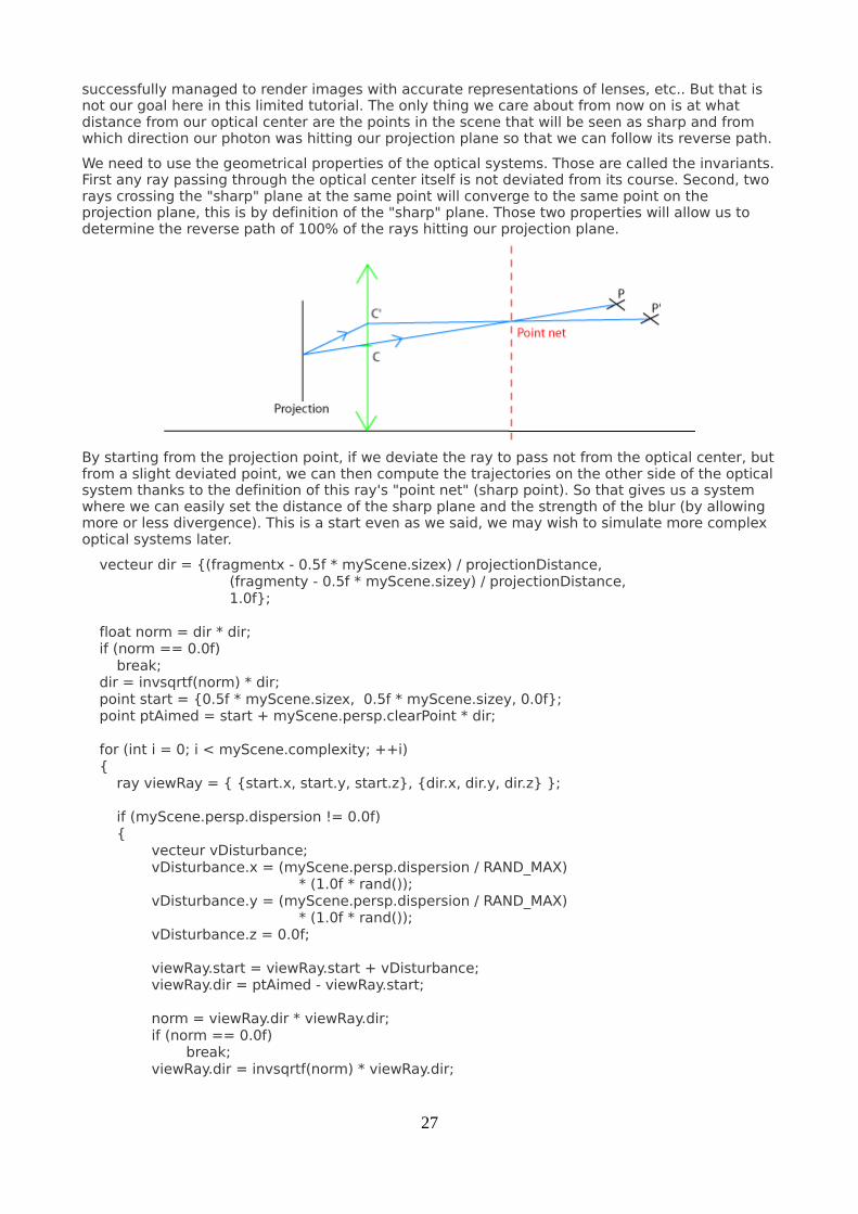
successfully managed to render images with accurate representations of lenses, etc.. But that is not our goal here in this limited tutorial. The only thing we care about from now on is at what distance from our optical center are the points in the scene that will be seen as sharp and from which direction our photon was hitting our projection plane so that we can follow its reverse path.

We need to use the geometrical properties of the optical systems. Those are called the invariants. First any ray passing through the optical center itself is not deviated from its course. Second, two rays crossing the "sharp" plane at the same point will converge to the same point on the projection plane, this is by definition of the "sharp" plane. Those two properties will allow us to determine the reverse path of 100% of the rays hitting our projection plane.

By starting from the projection point, if we deviate the ray to pass not from the optical center, but from a slight deviated point, we can then compute the trajectories on the other side of the optical system thanks to the definition of this ray's "point net" (sharp point). So that gives us a system where we can easily set the distance of the sharp plane and the strength of the blur (by allowing more or less divergence). This is a start even as we said, we may wish to simulate more complex optical systems later.

vecteur dir = {(fragmentx - 0.5f * myScene.sizex) / projectionDistance, (fragmenty - 0.5f * myScene.sizey) / projectionDistance, 1.0f};

float norm = dir * dir; if (norm == 0.0f) break; dir = invsqrtf(norm) * dir; point start = {0.5f * myScene.sizex, 0.5f * myScene.sizey, 0.0f}; point ptAimed = start + myScene.persp.clearPoint * dir;

for (int i = 0; i < myScene.complexity; ++i) { ray viewRay = { {start.x, start.y, start.z}, {dir.x, dir.y, dir.z} };

if (myScene.persp.dispersion != 0.0f) { vecteur vDisturbance; vDisturbance.x = (myScene.persp.dispersion / RAND_MAX) * (1.0f * rand()); vDisturbance.y = (myScene.persp.dispersion / RAND_MAX) * (1.0f * rand()); vDisturbance.z = 0.0f;

viewRay.start = viewRay.start + vDisturbance; viewRay.dir = ptAimed - viewRay.start; norm = viewRay.dir * viewRay.dir; if (norm == 0.0f) break; viewRay.dir = invsqrtf(norm) * viewRay.dir;

27

} color rayResult = addRay (viewRay, myScene, context::getDefaultAir()); fTotalWeight += 1.0f; temp += rayResult; } temp = (1.0f / fTotalWeight) * temp;The scene file now contains additional perspective information. The one that interests us here is the dispersion shown above. If the dispersion is not zero, then we have to look for the ray exiting from the optical center and the position of the "ptAimed" that is the point that lays at the distance clearPoint on that existing undisturbed ray. Then we add some perturbation and we recompute the direction from the perturbed origin to the ptAimed who is one of our invariant. The more we do that per pixel (with the number defined as "complexity"), the more we approach reality with an infinitely large number of rays. Of course we need to find the right compromise, because each additional ray makes the render longer. It's possible that we could find a heuristic to eliminate some of the additional rays on pixels that do not benefit from the extra complexity but let's not worry about that right now.

The "virtual" distance to the projection plane is determined by the FOV (field of view) and by the size of the viewport.

// We do some extra maths here, because our parameters are implicit.// The scene file contained the horizontal FOV (field of view)// and we have to deduct from it at what virtual distance // we can find our projection plane from the optical center.float projectionDistance = 0.0f;

if ((myScene.persp.type == perspective::conic) && myScene.persp.FOV > 0.0f && myScene.persp.FOV < 189.0f){ // This is a simple triangulation, from the FOV/2 // and the viewport horizontal size/2 projectionDistance = 0.5f * myScene.sizex / tanf (float(PIOVER180) * 0.5f * myScene.persp.FOV);}Ideally the coordinate of the scene should be independent of the resolution at which we render the scene but it is not here. In the future we should consider having a "normalized" coordinate system.

Here is the result of the depth of field effect with the sharp plane put at the same distance as the middle sphere :

28

And here is the result when the sharp plane is put at a farther distance. If the distance of the sharp plane is very large compared to the size of the aperture then only the landscape (at infinity) is seen as sharp here. For our eye and for a camera, "infinity" can be only a few feet away. It's only a matter of perception.

29

To get this level of quality without too much noise in the blur we need to send a large number of ray, more than one hundred per pixel in the image above. The time needed to render will almost scale linearly with the number of rays : if it takes one minute with one ray per pixel, then it will take one hundred minutes with one hundred rays per pixel. Of course this image took less (around several minutes at the time). Your mileage may vary, it all depends on the complexity of the scene, the amount of optimization that you could put into the renderer and of course of the performance of the CPU you're running it on.

The contribution of all the rays for a pixel are added together before the exposure and gamma correction took place. This is unlike the antialiasing computation. The main reason would be that the blur is the result of the addition of all photons before they hit the eye or the photosensitive area. In practice a very bright but blurry point one would leave a bigger trace on the image than a darker one. This is not a recent discovery as already painters like Vermeer exploited that small details to improve the rendering of their paintings. Vermeer like other people at his time had access to the dark chamber (camera oscura) which profoundly changed the perception of lighting itself.

Isosurfaces (blobs)

A iso-surface is a non planar surface that is defined mathematically like the set of points where a field of varying potential have the exact same value. The field has to be varying continuously else the definition does not constitute a surface. We suppose this field of scalar has the following properties :

- the fields that we consider are additive. That means that we have the field created by a source A, and the field created by the source B, if we put those two sources together, then the resulting field is simply the addition in each point of the space of the field A and the field B. In practice a lot of fields in real life acts this way. This is true for the magnetic field, the electric field and the

30

gravitational field, so the domain is well known. So if we wanted to represent an iso-gravitational surface we could use this method or a similar one.

- the potential field value when the source is a single point is well known. The potential is simply the inverse to the square distance to the source point. Thanks to this and the property above we can easily define the potential field created by N source points.

- this isn't a property but a mere discovered truth. We don't need a perfectly accurate representation of the iso-surface. We allow approximations in the rendering.

Below is a representation of 2D iso-potential curves (in red). Actually this image represents the field of three identical attractors in a gravitational field. Each single red line represents the iso-potential for a different value, in blue, we have the direction of the gradient of the scalar field. The gradient in that case is also the direction of the gravitational force.

What are the justifications for the above properties ? There is none. This is just one possible definitions for a blob you will probably be able to find other ones. Also you should note that for a single given source point, the iso-potential surfaces form a spherical shape. Only if there is a second (third, etc.) source in the area is the sphere deformed. That's why we'll sometimes see our blobs being called meta-balls. They are like spherical balls until they are close from each other, in which case they tend to fusion, as their potential fields add up.

Now let's examine our code implementation. Adding each potential and trying to resolve directly the potential = constant equation will be a bit difficult. Actually we'll end up with the resolution of polynomial equations of the nth degree but those will exceed what we want to do for our series of article. What we'll do instead is go the approximate way, but hopefully close enough for our limited scenes.

If we take the potential function f(r) = 1/r^2, we can approximate this rational function as a set of linear functions instead each of them operating on a different subdivision of space. If we divide the space around each source point with concentric spheres, between two concentric sphere we have the value 1/r^2 being close to a linear function f(r^2) = a*r^2 + b. Plus as we go further along the radius, at some point the potential for that source point becomes so close to zero that it has no chance to contribute to the iso-surface. Outside of that sphere, it's as if only the N-1 other source points contributed. This is an easy optimization that we can apply to quickly cull source points. The image below illustrate how our 1/r^2 function gets approximated by a series of linear function in r^2.

31

The image below illustrates how our view ray has to go through our field of potential. The potential function is null at the start, so the coefficients a, b, c are zero, zero, zero. Then it hits the first outer sphere. At this point with our approximation from above, the 1/r^2 potential becomes a polynomial of the first degree in r^2, r being defined as the distance that is between a point on our ray and the point that is the first source. This squared distance can be expressed in term of t, the arithmetic distance along our ray. This becomes then a polynomial function of the second degree in terms of t a1*t^2+b1*t+c1. We can then solves the equation a1*t^2+b1*t+c1 = constant to see if the ray has hit the iso-surface in that zone. Luckily for us it's a second degree equation with t as an unknown so very easy to solve (same complexity as our ray/sphere intersection described in the first page). We have to do that same intersection test for each new zone that the ray will encounter. Each zone is delimited by a sphere, that sphere will modify the equation by adding or subtracting a few terms but never by changing the shape of the equation. In fact we have very good features designed in that guarantee that the solution to our equation will be a continuous iso-potential surface.

So here follows the source code. Before doing the intersection test with the iso-surface we have to do the intersection tests with the concentric spheres. We'll have to determine how each intersection is sorted along the view ray, and how much each one contributes to the final equation. We'll have precomputed the contribution of each zone in a static array to accelerate the computation (those values stay constant for the whole scene).

for (unsigned int i= 0; i < b.centerList.size(); i++){ point currentPoint = b.centerList[i];

32

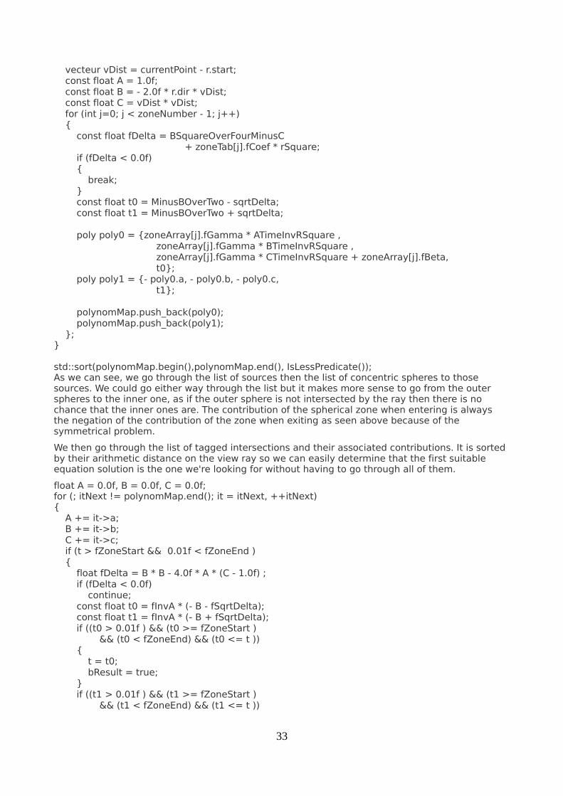
vecteur vDist = currentPoint - r.start; const float A = 1.0f; const float B = - 2.0f * r.dir * vDist; const float C = vDist * vDist; for (int j=0; j < zoneNumber - 1; j++) { const float fDelta = BSquareOverFourMinusC + zoneTab[j].fCoef * rSquare; if (fDelta < 0.0f) { break; } const float t0 = MinusBOverTwo - sqrtDelta; const float t1 = MinusBOverTwo + sqrtDelta;

poly poly0 = {zoneArray[j].fGamma * ATimeInvRSquare , zoneArray[j].fGamma * BTimeInvRSquare , zoneArray[j].fGamma * CTimeInvRSquare + zoneArray[j].fBeta, t0}; poly poly1 = {- poly0.a, - poly0.b, - poly0.c, t1}; polynomMap.push_back(poly0); polynomMap.push_back(poly1); };}

std::sort(polynomMap.begin(),polynomMap.end(), IsLessPredicate());As we can see, we go through the list of sources then the list of concentric spheres to those sources. We could go either way through the list but it makes more sense to go from the outer spheres to the inner one, as if the outer sphere is not intersected by the ray then there is no chance that the inner ones are. The contribution of the spherical zone when entering is always the negation of the contribution of the zone when exiting as seen above because of the symmetrical problem.

We then go through the list of tagged intersections and their associated contributions. It is sorted by their arithmetic distance on the view ray so we can easily determine that the first suitable equation solution is the one we're looking for without having to go through all of them.

float A = 0.0f, B = 0.0f, C = 0.0f;for (; itNext != polynomMap.end(); it = itNext, ++itNext){ A += it->a; B += it->b; C += it->c; if (t > fZoneStart && 0.01f < fZoneEnd ) { float fDelta = B * B - 4.0f * A * (C - 1.0f) ; if (fDelta < 0.0f) continue; const float t0 = fInvA * (- B - fSqrtDelta); const float t1 = fInvA * (- B + fSqrtDelta); if ((t0 > 0.01f ) && (t0 >= fZoneStart ) && (t0 < fZoneEnd) && (t0 <= t )) { t = t0; bResult = true; } if ((t1 > 0.01f ) && (t1 >= fZoneStart ) && (t1 < fZoneEnd) && (t1 <= t ))

33

{ t = t1; bResult = true; } if (bResult) return true; }}return false;Once the intersection point found, we have to compare it to the intersection point of other objects in the scene of course. If that's the one that is closer to the starting point we'll then have to do our lighting computation on that point. We have the point coordinates but we still need the normal to the surface in order to do the lighting, reflection and refraction. I've seen some people suggest to do the weighted average of all normals of the spheres around the source. But we can do way better than that, because of a nice property of the iso-potential surface. In the case of a surface defined at the points where potential=constant, then the normal to that surface is in the same direction as the gradient of the potential field. Below express as a mathematical expression :

The gradient of a potential field in 1/r^2 being a well known entity, we have the following code to compute the gradient of the sum of a couple of 1/r^2 fields :

vecteur gradient = {0.0f,0.0f,0.0f};float fRSquare = b.size * b.size;for (unsigned int i= 0; i < b.centerList.size(); i++){ vecteur normal = pos - b.centerList[i]; float fDistSquare = normal * normal; if (fDistSquare <= 0.001f) continue; float fDistFour = fDistSquare * fDistSquare; normal = (fRSquare/fDistFour) * normal;

gradient = gradient + normal;}After all those computations, here what we obtain when we combine three source points :

34

Fresnel and transparent volumes

Some materials have the property that they transmit the light really well (glass, water etc.) but affect its progression, which leads to two phenomenon. One phenomenon is the refraction, the ray of light is propagated but is deviated from its original trajectory. The deviation is controlled by a simple law that was first formulated by Descartes and Snell.

In short, if ThetaI is the incident angle that the view ray (or the light ray) does with the normal to the surface, then we have ThetaT, the angle that the transmitted ray does with the normal. ThetaT and ThetaI are part of the following equation : n2 * sin(ThetaT) = n1 * sin(ThetaI). This is the famous Snell-Descartes law.

n is called the refraction index of the medium. It is a variable with no unit that is computed for each medium by its relation to the void itself. The void is given a refraction index of 1. n1 is on the incident side and n2 is on the transmission side. Of course since the problem is totally symmetrical, you can easily swap the value of ThetaI and ThetaT, n1 and n2. In classical optics there is no difference between incoming ray and a ray that goes away. That's why we can consider light rays and view rays as similar objects.

The above relation cannot work for all values of ThetaI and ThetaT though. If n1 > n2, then there are some possible ThetaI values for which there is no corresponding ThetaT (because sin(ThetaT) cannot be bigger than one). What it means in practice is that in the real world, when the ThetaI exceeds a certain value then there is simply no transmission possible.

The second effect that those transparent surface cause is to reflect a part of their incident light. This reflection is similar to the mirror reflection we had described in the previous pages, that is the reflected ray is the symmetrical ray to the incident ray with the normal as the axis of symmetry. But what's different is that the intensity of the reflected ray will vary according to the amount of light that was transmitted by refraction.

What is the amount of light that is transmitted and the amount that is reflected ? That's where Fresnel comes into play. The Fresnel effect is a complex mechanism that needs to take into account the ondulatory nature of light (light is a wave). Until now we've treated all surfaces as perfect mirror. A surface of a perfect mirror has loaded particles that will be excited by the light and generate a perfect counter wave that will seemingly cause the ray to go towards the reflected direction.

But most surfaces are not perfect mirrors. Most of the time they will reflect light a little bit at some angles, and be more reflective at some other angles. That's the case of materials such as water and glass. But it's also the case for a lot of materials that are not even transparent, a paper sheet for example will reflect light that comes at a grazing angle and will absorb and re-diffuse the rest (according to the Lambert's formula). Wood, or ceramic would behave similarly too. The amount of light that is reflected in one direction depending on the angle of incidence is called the reflectance.

For a surface that reacts to an incident electromagnetic field there are two types of reflectance depending on the polarity of light. Polarity is the orientation along whom the electric and the magnetic fields are oscillating. For a given incident ray we can basically separate it into two separate rays, one where the photons are oriented along the axis parallel to the surface and one where the photons are oriented along a perpendicular axis. For a light that was not previously

35

polarized, the intensity of each kind is divided in half and half. Of course for simplification reaons we forget about the polarity of light and we simply take the average of the reflectance computed for parallel and perpendicular photons.

float fViewProjection = viewRay.dir * vNormal;fCosThetaI = fabsf(fViewProjection); fSinThetaI = sqrtf(1 - fCosThetaI * fCosThetaI);fSinThetaT = (fDensity1 / fDensity2) * fSinThetaI;if (fSinThetaT * fSinThetaT > 0.9999f){ fReflectance = 1.0f ; // pure reflectance at grazing angle fCosThetaT = 0.0f;}else{ fCosThetaT = sqrtf(1 - fSinThetaT * fSinThetaT); float fReflectanceOrtho = (fDensity2 * fCosThetaT - fDensity1 * fCosThetaI ) / (fDensity2 * fCosThetaT + fDensity1 * fCosThetaI); fReflectanceOrtho = fReflectanceOrtho * fReflectanceOrtho; float fReflectanceParal = (fDensity1 * fCosThetaT - fDensity2 * fCosThetaI ) / (fDensity1 * fCosThetaT + fDensity2 * fCosThetaI); fReflectanceParal = fReflectanceParal * fReflectanceParal;

fReflectance = 0.5f * (fReflectanceOrtho + fReflectanceParal);}Then we have to modify slightly the code that computes the lighting and the rest. First if the reflection and refraction coefficients are both equal to one then we forget about the any other lighting because in that case that means that all the light intensity is either reflected or transmitted. Then we have to follow the view ray after it hit the surface. Before that point we had very limited choice we were either reflected or stopped. Here we have a third choice appearing. The C++ language and the computer execution being sequential in nature we cannot follow all choices at the same time. We can use recursion and store temporary choices on the C++ stack or do something else. In our code we decided to do something else but it's pretty arbitrary so you shouldn't think that's the only solution. So instead of following the full tree of solutions, I only follow one ray at a time even if the choices made me diverge from another possible path. How can we account for BOTH reflection and refraction in this case ? We'll use the fact that we've already shot a lot of rays for the depth of field effect and that we can evaluate a lot of different paths by shooting rays and varying randomly (or not) the path taken in each ray. I call that the "Russian roulette", because at each divergence I pick randomly based on some "importance" heuristic which road my ray will take.

We need a lot of samples per pixels but we have to acknowledge that some samples will contribute more to the final image because they contributed more light. This leads to our implementation of importance sampling. The reflectance and transmittance we've computed above have then to be taken as "probabilities" that a given ray will take one path vs the other.

Here's what we have when we've rewritten those ideas in C++ :

float fRoulette = (1.0f / RAND_MAX) * rand();

if (fRoulette <= fReflectance){ // rays are either reflected, .. coef *= currentMat.reflection; viewRay.start = ptHitPoint; viewRay.dir += fReflection * vNormal;}else if(fRoulette <= fReflectance + fTransmittance){ // ..transmitted.. coef *= currentMat.refraction;

36

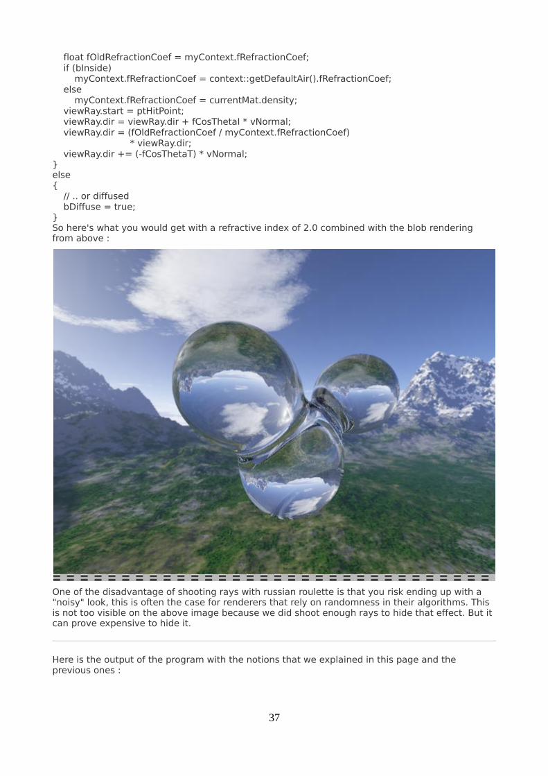
float fOldRefractionCoef = myContext.fRefractionCoef; if (bInside) myContext.fRefractionCoef = context::getDefaultAir().fRefractionCoef; else myContext.fRefractionCoef = currentMat.density; viewRay.start = ptHitPoint; viewRay.dir = viewRay.dir + fCosThetaI * vNormal; viewRay.dir = (fOldRefractionCoef / myContext.fRefractionCoef) * viewRay.dir; viewRay.dir += (-fCosThetaT) * vNormal;}else{ // .. or diffused bDiffuse = true;}So here's what you would get with a refractive index of 2.0 combined with the blob rendering from above :

One of the disadvantage of shooting rays with russian roulette is that you risk ending up with a "noisy" look, this is often the case for renderers that rely on randomness in their algorithms. This is not too visible on the above image because we did shoot enough rays to hide that effect. But it can prove expensive to hide it.

Here is the output of the program with the notions that we explained in this page and the previous ones :

37

For this page and the following ones you will also need the extra files in the archive called textures.rar (3 MB). It contains the cube map files used to render those images.

38