Toolbox for the Modeling and Analysis of Thermodynamic Systems (T-MATS)

User’s Guide

Jeffryes W. ChapmanVantage Partners, LLC,Cleveland, OH 44135

Thomas M. LavelleNASA Glenn Research Center,

Cleveland, OH 44135

Ryan D. MayVantage Partners, LLC,Cleveland, OH 44135

Jonathan S. Litt, and Ten-Huei GuoNASA Glenn Research Center,

Cleveland, OH 44135

Revisions list

Version Date User Descriptionv1.0 2013-11-15 JWC Initial Releasev1.1 2014-10-01 JWC Added T-MATS Cantera updatesv1.1.2 2016-01-15 JWC Added T-MATS callable functions and publications sections.

Moved Cantera section. Corrected PR scalar definition. Corrected equation 1 to reflect the Jacobian matrix. Updated Introduction. Added sections for T-MATS tools and version compatibility.

V1.1.3 2016-05-20 JWC Updated Tools section to and Callable MATLAB functions. Additionally created a new version compatibility section for version 1.1.3.

V1.2 2017-11-08 JWC Made various updates. Major updates include, adding volume and heat transfer libraries, adding NPSS to T-MATS conversion tool, updating T-MATS code example, updating references, and adding version information.

V1.2.1 2018-03-16 JWC Updated Cantera links to current github location.

1

Table of Contents1 Introduction......................................................................................................................................................5

1.1 Identification............................................................................................................................................5

1.2 Notation....................................................................................................................................................6

1.3 System Overview......................................................................................................................................6

1.4 T-MATS quick start guide........................................................................................................................6

1.4.1 Installing T-MATS...........................................................................................................................6

1.4.2 Un-installing T-MATS.....................................................................................................................7

1.4.3 T-MATS examples...........................................................................................................................8

1.4.4 Block Help........................................................................................................................................8

2 T-MATS Library Structure.................................................................................................................................9

3 T-MATS Tools..................................................................................................................................................10

3.1 T-MATS Tools..........................................................................................................................................10

3.1.1 GasTableBuilder.............................................................................................................................10

3.1.2 MapGeneration_Tools....................................................................................................................10

3.1.3 NPSS to TMATS conversion tool...................................................................................................10

3.2 T-MATS Simulink Tools...........................................................................................................................10

3.2.1 GF_Convert....................................................................................................................................10

3.2.2 Block Link Setup............................................................................................................................10

3.2.3 Set IDes..........................................................................................................................................11

4 Callable MATLAB Functions........................................................................................................................11

5 Cantera Integration.........................................................................................................................................12

5.1 Cantera Installation.................................................................................................................................12

5.2 Using T-MATS_Cantera Blocks and scripts...........................................................................................12

5.3 Interfacing with Cantera.........................................................................................................................15

6 T-MATS Simulation creation...........................................................................................................................18

6.1 Simulation Setup....................................................................................................................................18

6.2 T-MATS formatting...............................................................................................................................20

6.2.1 Color Coding..................................................................................................................................20

6.2.2 Simulink Wiring.............................................................................................................................20

6.2.3 Mask format....................................................................................................................................21

2

6.2.4 S-Functions.....................................................................................................................................23

6.3 Units.......................................................................................................................................................23

6.4 Solver Setup...........................................................................................................................................23

6.5 Turbomachinery Plant Setup..................................................................................................................24

6.5.1 Independent and Dependent variables.............................................................................................24

6.5.2 Maps...............................................................................................................................................25

6.5.3 Compressor Variable Geometries (IGVs and VSVs)......................................................................29

6.5.4 Bleeds and Air Bypass....................................................................................................................29

6.5.5 Turbofan modeling options.............................................................................................................31

6.5.6 iDesign............................................................................................................................................32

7 Customization.................................................................................................................................................32

7.1 Library Blocks........................................................................................................................................33

7.1.1 Creating new Simulink Library Browser folders............................................................................33

7.2 S-functions..............................................................................................................................................33

7.3 Tool Creation..........................................................................................................................................34

8 Troubleshooting T-MATS................................................................................................................................35

8.1 Convergence “Errors”.............................................................................................................................35

8.2 Crashing.................................................................................................................................................36

9 Version Compatibility.....................................................................................................................................37

9.1 Version 1.1.2...........................................................................................................................................37

9.2 Version 1.1.3...........................................................................................................................................38

9.3 Version 1.2..............................................................................................................................................38

10 Related Publications...................................................................................................................................39

11 T-MATS Tutorials........................................................................................................................................40

11.1 T-MATS example 1: Newton-Raphson Equation Solver........................................................................40

11.2 T-MATS example 2: Example_GasTurbine_SS.....................................................................................43

11.2.1 Creating the Gas Turbine Plant.......................................................................................................43

11.2.2 Plant Solver integration and plant inputs........................................................................................46

11.3 T-MATS example 3: Example_GasTurbine_Dyn...................................................................................49

11.3.1 General Architecture.......................................................................................................................49

11.3.2 Adding control to the simulation....................................................................................................53

11.3.3 Plant interface with outer loop systems...........................................................................................55

3

11.3.4 Advanced Simulation Structure and Formatting.............................................................................55

12 Acknowledgments......................................................................................................................................57

13 Appendix A.................................................................................................................................................58

Index of FiguresFigure 1. T-MATS/Cantera block hierarchy...........................................................................................................14Figure 2. Sample simulation architecture for a dynamic system.............................................................................18Figure 3. Sample T-MATS function block parameters mask..................................................................................20Figure 4. Sample T-MATS function block parameters mask with vectored inputs and checkboxes......................21Figure 5. Sample turbojet block diagram................................................................................................................23Figure 6. Sample compressor map (pressure ratio vs. corrected flow)...................................................................25Figure 7. Sample compressor map (efficiency vs. corrected flow).........................................................................26Figure 8. Sample turbine map (corrected flow vs. pressure ratio)..........................................................................27Figure 9. Sample turbine map (efficiency vs. pressure ratio)..................................................................................27Figure 10. Sample fan model creation schemes for a gas turbine with bypass.......................................................30Figure 11: Sample MATLAB internal problem message.......................................................................................35Figure 11. Model configuration parameters setup..................................................................................................40Figure 13. Run equation solver...............................................................................................................................41Figure 14. Gas turbine plant...................................................................................................................................44Figure 15. Steady-state solver setup.......................................................................................................................46Figure 16. Iterative NR Solver w JacobianCalc wiring...................................................................49Figure 17. Dynamic gas turbine simple “outer” loop..............................................................................................51Figure 18. Dynamic gas turbine with controller.....................................................................................................53

Index of TablesTable 1. T-MATS user’s manual notation................................................................................................................6Table 2. TMATS thermodynamic functions...........................................................................................................11Table 3. T-MATS_Cantera flow vector structure for Simulink..............................................................................12Table 4. Package TMATSC functions and classes.................................................................................................15Table 5. Class TMATSC.FlowDef methods, Cantera interface functions..............................................................16Table 6. T-MATS color coding..............................................................................................................................19Table 7. T-MATS default units and common constants.........................................................................................22Table 8. Dynamic turbofan model independent and dependent variables...............................................................24Table 9. Compressor map equations.......................................................................................................................26Table 10. Compressor map equations.....................................................................................................................28Table 11. T-MATS library file structure.................................................................................................................31Table 12. Steady-state turbofan engine example, unused outputs...........................................................................42Table 13. Example 2 convergence outputs.............................................................................................................47

4

1 IntroductionThe Toolbox for the Modeling and Analysis of Thermodynamic Systems (T-MATS) is a Simulink toolbox intended for use in the modeling and simulation of thermodynamic systems and their controls. The package contains generic thermodynamic and controls components that may be combined with a variable input iterative solver and optimization algorithm to create complex systems to meet the needs of a developer.

The goal of the T-MATS software is to provide a toolbox for the development of thermodynamic system models, which contains a simulation framework, multi-loop solver techniques, and modular thermodynamic simulation blocks. While much of the capability in T-MATS is in transient thermodynamic simulation, the developer’s main interests are in aero-thermal applications; as such, one highlight of the T-MATS software package is the turbomachinery block set. This set of Simulink blocks gives a developer the tools required to create virtually any steady-state or dynamic turbomachinery simulation, e.g., a gas turbine simulation. In systems where the control or other related systems are modeled in MATLAB/Simulink, the T-MATS developer has the ability to create the complete system in a single tool.

T-MATS turbomachinery blocks were created using a philosophy that combines the understandability and logic of physics-based models with the accuracy and tunability of empirically-developed models. This user’s guide is written with the assumption that the user is familiar with modeling thermodynamic systems, and a user is encouraged to see the referenced documentation1,2 for a review of general thermodynamic and modeling principles before building a simulation.

T-MATS is written in MATLAB®/Simulink® v2015aSP1 (The Mathworks, Inc.), is open source, and is intended for use by industry, government, and academia. All T-MATS equations were developed from public sources and all default maps and constants provided in the T-MATS software package are nonproprietary and available to the public.3 The software is released under the Apache V2.0 license agreement. License terms and conditions can be found at http://www.apache.org/licenses/LICENSE-2.0.

1.1 IdentificationThe T-MATS user’s guide applies to version 1.2 of the T-MATS software package, as developed by NASA Glenn Research Center. The package consists of a T-MATS Simulink library containing the following sub-libraries: Effectors and Controls, Heat Transfer, Numerical Methods, Solver, Thermo, Thermo_Cantera, Turbomachinery, Turbomachinery_Cantera, and Volume. In addition, the T-MATS package contains development tools, “T-MATS tools,” as well as examples to demonstrate how systems may be created using the Simulink libraries.

1 http://www2.chem.umd.edu/thermobook/ :Referenced as of 9/2013 2 Jones, S. M.,”Steady-State Modeling of Gas Turbine Engines using the Numerical Propulsion System Simulation Code,” GT2010-22350, ASME Turbo Expo, Glasgow, UK, June 14-18, 2010.3 Jones, S.M.,”An Introduction to Thermodynamic Performance Analysis of Aircraft Gas Turbine Engine Cycles Using the Numerical Propulsion System Simulation,” NASA/TM-2007-214690, March 2007.

5

1.2 NotationThe notation summarized in Table 1 will be used throughout the T-MATS User’s Guide.

Table 1. T-MATS user’s manual notation.

Type DefinitionCourier Font MATLAB function, Simulink blocks, or

code (i.e., Simulink: From block)Times New Roman Font Italics Variables (i.e., f(x)) or file names, block

input/outputArial Font File Paths (i.e., TMATS_Library\MEX)Platform: Name block Signify what library a block is taken from

(i.e., Simulink: From block)

1.3 System OverviewThe Toolbox for the Modeling and Analysis of Thermodynamic Systems (T-MATS) is a generic thermodynamic simulation system built in MATLAB/Simulink. Developed to use graphical-based simulation techniques to meet the requirements of industry professionals as well as academics, T-MATS combines generic thermodynamic and controls modeling capability with a numerical iterative solver to create a framework for the creation of complex thermodynamic system simulations. Numerical methods utilized by T-MATS include Newton-Raphson iterative solving techniques and Jacobian calculation techniques.

1.4 T-MATS quick start guide

1.4.1 Installing T-MATSTo install T-MATS execute the following steps:

1. Download T-MATS from the GIT server https://github.com/nasa/T-MATS /releases , click the green download button for the latest version, and extract the files to a folder that can be accessed by MATLAB, ensuring there are no spaces in the path name. Note that T-MATS was developed in the Microsoft Windows 7 operating system using MATLAB (baseline v2015aSP1) and Microsoft Software Development Kit (SDK) 7.1; it is not guaranteed to work on other operating systems, with other MATLAB versions, or with other compilers. For a full description of compilers compatible with MATLAB 2015a see http://www.mathworks.com/support/compilers/R2015a/index.html?sec=win64.

2. Navigate to the directory of the desired released version of T-MATS in the downloaded zip file, TMATS_vXX, in MATLAB.

3. Run Install_TMATS.m; this will set up the paths for T-MATS as well as create the mex files.If the user does not have elevated privileges, paths may not have been saved properly. If the paths have not been saved, new paths can manually be added to the pathdef.m file. Open the “Set Path” window by clicking on the “Set Path” button in the MATLAB toolbar on the HOME tab and add the paths (\TMATS_Library, \TMATS_Library\MEX, \TMATS_Library\TMATS_Support, and \TMATS_Tools) to the list. Click “Save” to save the path definitions; a message will pop up warning that administrator privileges are required and providing the option to instead save the paths to a new pathdef.m file. Save

6

this file to a location on the MATLAB path. Note: this process will save the current path list; before saving, it should be verified that no unintended paths are on the list. If a temporary install of T-MATS is desired the temporary install button can be selected on the install popup. Installing with temporary install will not save the new paths.

4. To add the T-MATS Simulink tools to the Simulink toolbar, create the MATLAB file, startup.m, with the following lines of code:

load_simulinkMenu_customization_TMATS

The startup.m file may be saved anywhere on the MATLAB path, and these lines function to load T-MATS editing tools to the Simulink window each time MATLAB is opened. If a startup.m file already exists, just add the above lines of code.If, during MATLAB startup, a warning is displayed notifying the user that Menu_customization_TMATS.m cannot be found, it is probable that the T-MATS paths have not been added properly in MATLAB. The most common reasons for missing path definitions are that either the T-MATS paths were not loaded into the pathdef file (see step 3 to solve this issue) or the modified startup.m file is being used by a version of MATLAB that T-MATS was not installed on. The warning messages can be removed by either installing T-MATS on the other version or by placing the startup.m file in a path used only by the desired MATLAB version. It should be noted that, while these warnings may be annoying, they will have no effect on the performance or functionality of MATLAB if T-MATS is not used.

5. Optionally, if a user wishes to use the Cantera integrated T-MATS blocks, the MATLAB Cantera toolbox will need to be installed. Instructions detailing the installation process are detailed in Section 5.1.

At this point the T-MATS library installation is complete. T-MATS modules may be found in the Simulink Library Browser under the heading “TMATS.” The T-MATS Simulink tools may be found under “Diagram” in the Simulink model window menu bar.

1.4.2 Un-installing T-MATSTo remove T-MATS, execute the following steps:

1. Execute Uninstall_TMATS.m from the same location that Install_TMATS was run. (By default, these files are both located in the TMATS folder).

a. If paths were added manually to the pathdef.m file during installation, they must be removed manually by re-saving the pathdef.m file after the Uninstall_TMATS.m file has been run.

2. Remove the following lines from the startup.m file:

load_simulinkMenu_customization_TMATS

7

1.4.3 T-MATS examplesT-MATS includes a number of sample systems set up to help a user gain insight into how to use the T-MATS library to simulate thermodynamic systems. To gain access to these examples, navigate to the Examples folder under TMATS_Examples and run TMATS_Run_Example.m. A selection of different examples will be listed in the MATLAB window (as shown below); the user can then indicate the number corresponding to the example to open. An alternate way to open an example is to navigate directly to the folder containing the example and run the *_setup_everything.m file (or by opening the *.slx file, in cases where a setup file does not exist).

>> run('C:\Builds\TMATS\TMATS_Examples\TMATS_Run_Example.m')Select the enumeration of the T-MATS Example to be setup:1) NewtonRaphson_Equation_Solver2) Steady State GasTurbine3) Dynamic GasTurbine4) Steady State Dual Spool High Bypass Engine JT9D5) Dynamic Dual Spool High Bypass Engine JT9D6) Steady State JT9D, Cantera7) Cycle Model8) Linearization Examples9) Volume Example10) Cancel Setup

The *_setup_everything.m script will execute every command necessary to set up that particular example, which may include any of the following: loading variables to the workspace, creating paths, loading busses, and opening the Simulink model. The paths can be removed by running the corresponding *_Example_cleanup.m file.

1.4.4 Block Help Each T-MATS module contains a help file that explains the particulars of how to set up that block, therefore the low level functionality of each block will not be discussed in this document. Additional documentation can be found in the block guide located in the T-MATS base directory.

8

2 T-MATS Library StructureThe T-MATS Library, as displayed in the Simulink Library Browser, contains four sub-libraries: Effectors and Controls, Numerical Methods, Solver, Thermo, Thermo_Cantera, Turbomachinery, Turbomachinery_Cantera and Volume.

1. Effectors and Controls: This sub-library contains the building blocks of the outermost loop of a simulation. The library blocks are simple representations of effector and control system components. Depending on the fidelity requirements of the simulation, it may be necessary to develop more complex models.

2. Heat Transfer: This sub-library contains building blocks to solve the heat flow problem using various methods, including 0-D lumped mass and 1-D methods using various discretization techniques.

3. Numerical Methods: This sub-library contains the most basic building blocks of the numerical solvers required to simulate a T-MATS system. These blocks are very generic and can be used to create iterative solvers for a wide range of systems, even outside of T-MATS.

4. Solver: This sub-library contains blocks that simplify simulation creation, including hybrid blocks, comprised of blocks from the “Numerical Methods” sub-library, and blocks that are useful for general simulation development.

5. Thermo: This sub-library contains blocks for general Thermodynamic systems. Many of the blocks located within this sub-library may be used in other TMATS libraries.

6. Thermo_Cantera: This sub-library contains general use Thermodynamic blocks that require the Cantera software package to run.

7. Turbomachinery: This sub-library contains the building blocks necessary to create a gas turbine model for simulation. The blocks are based on basic thermodynamic equations and principles, and use a series of maps that define the characteristics of the system being modeled. The default maps and constants in T-MATS are intended only for demonstration.

8. Turbomachinery_Cantera: This sub-library contains turbomachinery blocks that require the Cantera software package to run.

9. Volume: This sub-library contains building blocks dedicated to solving the 1-D flow problem. And is based on thermodynamic table lookups, independent of baseline T-MATS, for fluid properties.

T-MATS is intended to be an environment for building thermodynamic simulations in Simulink with the goal of dynamic analysis and controls design. The sub-libraries discussed above provide the basic building block of a simulation, however a user may be required to create new blocks, and/or tweak existing blocks, to meet his/her specific needs.

9

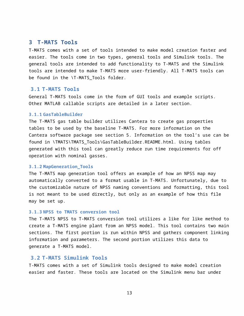
3 T-MATS ToolsT-MATS comes with a set of tools intended to make model creation faster and easier. The tools come in two types, general tools and Simulink tools. The general tools are intended to add functionality to T-MATS and the Simulink tools are intended to make T-MATS more user-friendly. All T-MATS tools can be found in the \T-MATS_Tools folder.

3.1 T-MATS ToolsGeneral T-MATS tools come in the form of GUI tools and example scripts. Other MATLAB callable scripts are detailed in a later section.

3.1.1 GasTableBuilderThe T-MATS gas table builder utilizes Cantera to create gas properties tables to be used by the baseline T-MATS. For more information on the Cantera software package see section 5. Information on the tool’s use can be found in \TMATS\TMATS_Tools\GasTableBuilder.README.html. Using tables generated with this tool can greatly reduce run time requirements for off operation with nominal gasses.

3.1.2 MapGeneration_ToolsThe T-MATS map generation tool offers an example of how an NPSS map may automatically converted to a format usable in T-MATS. Unfortunately, due to the customizable nature of NPSS naming conventions and formatting, this tool is not meant to be used directly, but only as an example of how this file may be set up.

3.1.3 NPSS to TMATS conversion toolThe T-MATS NPSS to T-MATS conversion tool utilizes a like for like method to create a T-MATS engine plant from an NPSS model. This tool contains two main sections. The first portion is run within NPSS and gathers component linking information and parameters. The second portion utilizes this data to generate a T-MATS model.

3.2 T-MATS Simulink ToolsT-MATS comes with a set of Simulink tools designed to make model creation easier and faster. These tools are located on the Simulink menu bar under Diagram -> T-MATS Tools. Each tool will be described in the following sections.

3.2.1 GF_ConvertThe GF_Convert tool changes the selected Simulink: GoTo block into a Simulink: From block, or vice versa. It will also convert a Simulink: Outport into a Simulink: Inport and vice versa.

3.2.2 Block Link SetupBlock Link Setup will create Simulink: GoTo blocks and/or Simulink: From blocks that correspond to a particular subsystem’s inputs and outputs, and then connect them with wires. T-MATS blocks will be dealt with on a case-by-case basis, with blocks and connections created as appropriate for that particular block. In many cases, additional Simulink: GoTo or Simulink: From blocks will be created that are intended to be used in other parts of the simulation. The Block Link Setup tool may also be used to create a Simulink: Inport or Simulink: Output block for a selected Simulink: GoTo or Simulink: From block, or vice versa.

10

3.2.3 Set IDesSet Ides will look through the current diagram for blocks containing the variable iDesign_M and changes it to the value specified in the GUI. Note: this only works for the current diagram and if there are sub-models being used they much be changed separately.

4 Callable MATLAB FunctionsMuch of modeling in T-MATS is based on non-linear table lookups that contain information about the thermodynamic state of a material or fluid flow. These table lookups can be accessed via the C-code, MATLAB script or through the Simulink browser folder T-MATS\Thermo. By default these table lookups contain the thermodynamic properties of air and a hydrocarbon exhaust gas. The ratio between these components is defined as FAR. To work with alternate components the baseline tables must be updated. Once T-MATS has been installed, the TMATS class will give access to the MATLAB table lookup functions, as shown in Table 2. These commands can be accessed by using the syntax TMATS. (i.e. TMATS.h2t(h,FAR)) or by using “import TMATS.*” in the workspace or a MATLAB script. This information may also be accessed by typing “help TMATS” in the MATLAB command window.

Table 2. TMATS thermodynamic functions.

Function descriptionT = h2t(h,FAR) Determine temperature [R] based on enthalpy [BTU/lbm] and fuel to air

ratios = pt2s(P,T,FAR) Determine entropy [BTU/(lbm*R)] based on temperature [R], pressure

[psia], and fuel to air ratioT = sp2t(s,P,FAR) Determine temperature [R] based on entropy [BTU/(lbm*R)], pressure

[psia], and fuel to air ratioh = t2h(T,FAR) Determine enthalpy [BTU/lbm] based on temperature [R] and fuel to air

ratioDViewGUI Runs the T-MATS data viewer GUI. This GUI can run a Simulink

model, plot the steady-state data, plot the transient data, and/or set the iDesign_M variable as desired. Note: for this tool to work correctly T-MATS station must be output using the Simulink/ToWorkspace block with data set to TimeSeries and be included in a bus containing W,h,T,P, and FAR (default T-MATS GasPthChar bus). Functions that plot performance maps will search out map data automatically, however data on the map requires component Data bus outputs set up similarly. Execute command, help TMATS.DViewGUI, for more details.

PlotCMap(NcVec, WcArray, PRArray, EffArray)

Plot compressor map with Wc, PR, and Eff defined as a functions of Nc and Rline. Execute command, help TMATS.PlotCMap, for more details.

PlotTMap(NcVec, PRVec, WcArray, EffArray)

Plot turbine map with Wc and Eff defined as functions of Nc and PR. Execute command, help TMATS.PlotCMap, for more details.

SSplot(filename, StationVarVec) Calls the T-MATS steady state data viewer. Variable: filename denotes the Simulink diagram that generated the data, StationVarVec is a vector

11

of all outputs generated by the ToWorkspace blocks. Note: this tool will search for all Simulink/ToWorkspace blocks, verify they are in the form of T-MATS station data (Timeseries with W,h,P,T,FAR) then use that data to make set plots. It will also search for compressor and turbine blocks to create map plots and Data busses for placing data on the maps. Execute command, help TMATS.SSplot, for more details.

TDplot(filename) Calls the T-MATS transient data viewer. The variable, filename, is the Simulink diagram name that is generating the desired data. Note: this tool will search for all Simulink/ToWorkspace blocks, verify they are in the form of T-MATS station data (Timeseries with W,h,P,T,FAR) then use that data to make set plots. It will also search for compressor and turbine blocks to create map plots and Data busses for placing data on the maps. Execute command, help TMATS.TDplot, for more details.

It should be noted, Table 2 lists only T-MATS functions that do not make use of the Cantera package. For T-MATS functions that require the Cantera package, see section 5.

5 Cantera IntegrationSome T-MATS blocks have been integrated with the open source Cantera software package. As stated by the software documentation (http://cantera.github.io/docs/sphinx/html/index.html), “Cantera is a suite of object-oriented software tools for problems involving chemical kinetics, thermodynamics, and/or transport processes.” Integration of Cantera brings many new capabilities to T-MATS, including the use of off nominal fuels, alternate flow path gasses, etc. This is accomplished with the addition of a new MATLAB package that includes a Simulink sub-library (Turbomachinery_Cantera and Thermo_Cantera), scripts, and classes.

5.1 Cantera InstallationT-MATS_Cantera makes use of MATLAB scripts with Cantera functions built in, which are located within the \TMATS\TMATS_Library\MATLAB_Scripts\Cantera_Enabled folder. To use these scripts the Cantera Toolbox must be installed into MATLAB/Simulink. Instructions on how to install the Cantera package are located at the software homepage (https://github.com/Cantera/cantera and http://cantera.github.io/docs/sphinx/html/index.html ). It should be noted that T-MATS_Cantera was developed using the Cantera Toolbox version 1.0. Toolbox version numbers can be checked using the ver command in MATLAB.

5.2 Using T-MATS_Cantera Blocks and scriptsT-MATS blocks that utilize Cantera functions are located in the Simulink library browser under *_Cantera and Cantera enabled scripts are located in the TMATSC MATLAB package. Before a simulation containing T-MATS_Cantera blocks or scripts can be run, a global variable, fs, must be defined and the script canteraload.m located in the folder, TMATS\TMATS_Library\MATLAB_Scripts\Cantera_Enabled\+TMATSC, must be filled out.

The canteraload.m script defines the Name and Species of the flow streams. Currently there may be up to six flow types that each contain up to six molecule components. This information is organized into a 6×6 matrices with rows containing molecule types and columns containing their proportions by weight. Flow compositions are

12

determined from a 6×1 vector where each value relates to one row of the 6×6 matrix. For example, a flow composition vector of [1 0 0 0 0 0] would relate to Air comprised of: N2; 0.7547, O2; 0.232, and AR; 0.0128 as seen below (Note, all compositions are proportional by weight). In general the flow composition vector is generated automatically then used along with the Name and Species matrices to complete and execute Cantera functions. Because of this, Name and Species form must be consistent with Cantera function notation. Default definitions for Name and Species is located below and details generic air (row 1), water (row 2), and fuel (row 3). The remaining 3 rows have not been defined.

Name = { 'N2' 'O2' 'AR' '' '' '';... %Air'H2O' '' '' '' '' '';... %Water'CH2' 'CH' '' '' '' '';... %Fuel'' '' '' '' '' '';...'' '' '' '' '' '';...'' '' '' '' '' '' };

Species = { 0.7547 0.232 0.0128 0 0 0;... %Air1 0 0 0 0 0;... %Water0.922189 0.077811 0 0 0 0;... %Fuel0 0 0 0 0 0;...0 0 0 0 0 0;...0 0 0 0 0 0};

In addition to specifying the composition values for the flows, it is also important to create the Cantera phase object to allow Cantera to communicate with MATLAB appropriately. The phase object is defined by creating global variable fs in the MATLAB workspace. The variable fs must contain all necessary molecule types that are used in the load script presented above. Below is an example of the commands that may be used to declare fs.

global fsfs = importPhase('gri30.cti')

The Cantera function importPhase will import one phase from an input file, in this case gri30.cti. For T-MATS_Cantera Simulink blocks, flow information is transferred via a 25×1 vector that is defined as shown in Table 3. This vector contains detailed flow information that may be used for calculations or informational purposes inside and/or outside of T-MATS blocks. The class containing methods TMATSC.FlowDef and TMATSC.FlwVec defines names for the flow vector, and may be updated per user requirements. It should be noted that all communication between Cantera and MATLAB is handled with a MATLAB class, as described in the next section, and a flow vector is only required because Simulink is incompatible with classes.

Table 3. T-MATS_Cantera flow vector structure for Simulink.

13

14

# Variable Description1 W gas path flow [pps]2 s entropy [BTU/(lbm*degR)]3 Tt total temperature [degR]4 Pt total pressure [psia]5 ht enthalpy [BTM/lbm]6 rhot total density (rho) [lbm/ft^3]7 gamt total specific heat ratio (gamma)8 Ts static temperature [degR]9 Ps static pressure [psia]10 hs static enthalpy [BTU/lbm]11 rhos static density (rho) [lbm/ft^3]12 gams static specific heat ratio (gamma)13 Vflow flow velocity [ft/sec]14 MN Mach number15 A flow area [in^2]16-21 CompVal_TMATS Flow composition vector, see canteraload.m for

definition of the 6 matter types22-25 none future use

5.3 Interfacing with CanteraT-MATS blocks that utilize Cantera functions have been built in a hierarchical fashion to allow a user to update the blocks to a level with which they are familiar. Looking at Figure 1, a simulation may be created in Simulink using the set of T-MATS_Cantera blocks. These blocks consist of an M-S-function that calls MATLAB scripts written using the TMATSC MATLAB package. This MATLAB package consists of specialty scripts and a class called FlowDef that acts as a simplified interface with Cantera. When working with a design any of these levels may be adjusted to meet task requirements.

Figure 1. T-MATS/Cantera block hierarchy.

15

Cantera Commands

TMATSC package, FlowDef class(MATLAB script)

Functional script(MATLAB script)

T-MATS_Cantera Block(M-S-function)

Simulation(Simulink)

The TMATSC MATLAB package contains a class and functions that are used in the creation of the T-MATS Cantera block set and are summarized in Table 4. Functions located within the package offer file manipulation and reading scripts useful for manipulating data storage.

Table 4. Package TMATSC functions and classes.

Function descriptionObject = FlowDef() Flow object constructor (see Table 5)[val] = canteraload(RequestType) Returns Name or Species matrix to be used in Cantera

command generation.[effMap, WcMap] = PRmapFile(MapFileName, NcMap, PRmap)

Table lookup for effMap and WcMap

[effMap, PRMap, WcMap, StallMargin] = RlineMap(MapFileName, NcMap, Rline)

Table lookup for effMap, PRMap, WcMap, and StallMargin

[val] = getV(var, parent) Get a variable from the workspacesetV(var, parent, value) Set a variable to the workspace.[string] = stripchar(string) Remove’ \’, ‘/’, or ‘\o’ from a character string.

The class TMATSC.FlowDef offers the ability to create flow objects that contain all the flow information required for thermodynamic computations, as well as laying out a simplified interface with Cantera functions, as shown in Table 5. Interaction with the Simulink environment is accomplished with the generation of a flow vector, described in Table 3 above, based a flow object. TMATSC functions and class methods can be imported into a script by implementing the command “import TMATSC.*” or by placing TMATSC. or TMATSC.FlowDef. , respectively, before the command. This information may also be accessed by typing “help TMATSC” in the MATLAB command window.

16

Table 5. Class TMATSC.FlowDef methods, Cantera interface functions.

Class Method descriptionFlow object construction:flow_new = FlowDef() 0 input Creates empty TMATSC flow objectflow_new = FlowDef(FlowVector) 1 input. Flow constructor based on flow vector.flow_new = FlowDef(flow, compNN, W, Tt, Pt)

4 inputs. Create populated flow object with total values only (Total only, based on set_TP)

flow_new = FlowDef(flow, compNN, W, Ts, Ps, MN)

5 inputs. Create populated flow object (Total and Static, based on set_TsPsMN)

flow_new = CanSet(flow) Set flow object composition values to Cantera format (CompVal_Can based on CompVal_TMATS flow object value)

flow_new = CanSet(flow, compNN) Set flow object composition values to Cantera format (CompVal_Can based on input compNN, 6×1 vector)

Cantera interface functions:flow_new = flowadd(flow1, flow2) Add flow1 and flow2 together, conserving enthalpy and massflow_new = flowcopy(flow) Copy information from one flow to another flowmass_frac = getMassFraction(flow, c) Return mass fraction of compound c in the object flowflow_new = set_hP(flow, ht, Pt) Set total conditions based on flow, total enthalpy and total

pressureflow_new = set_MN1(flow) Set the static conditions to sonic flow based on flow

conditionsflow_new = set_Ps(flow, Ps) Set the static conditions based on flow and static pressureflow_new = set_SP(flow, S, Pt) Set the total conditions based on flow and input entropy and

total pressureflow_new = set_TP(flow, Tt, Pt) Set the total conditions based on flow, total temperature, and

total pressureflow_new = set_TsPsMN(flow, Ts, Ps, MN) Set the conditions based on flow, static temperature, static

pressure, and Mach numberFlow object manual set functions:flow_new = TotalSet(flow, s, Tt, Pt, ht, rhot, gamt)

Manually sets total variables in flow object

flow_new = StaticSet(flow, Ts, Ps,hs, rhos, gams)

Manually sets static variables in flow object

flow_new = SpeedSet(flow, MN, A, Vflow) Manually sets speed variables in flow objectflow_new = SClr(flow) Clears all static variables in a flow objectflow_vector = FlwVec(flow) Creates 25×1 flow vector

To create an empty flow object, the following code can be executed in the MATLAB command prompt:

NewFlowObject = TMATSC.FlowDef();

Alternatively, a Cantera flow vector, as described in Table 3 , can be used to generate a defined flow object as shown below:

17

NewFlowObject = TMATSC.FlowDef(Flow_Vector);

The flow vector may be regenerated from the flow object using the FlwVec command:

FlowVector = FlwVec(FlowObjectName);

A good rule of thumb when choosing to use T-MATS_Cantera flow vectors or flow objects, is that a flow object created from the flow class should be used when working with the MATLAB scripting language, and the flow vector should be used only when transferring data out of Simulink blocks. It should be noted that when filling in a flow object manually, the TMATSC.CanSet method must be run after the CompVal_TMATS vector property has been set to automatically generate the CompVal_Can property, which is required by Cantera commands.

6 T-MATS Simulation creation

6.1 Simulation SetupIn many thermodynamic systems, the inputs to each component alone are not enough to determine how the system will respond. For example, the mass flow rate and pressure ratio across a compressor are not unique for a given shaft speed. In order to resolve this, a compressor map is used to solve for incoming flow to the compressor block. This calculated compressor flow and the actual incoming flow are then compared to calculate a flow error. During simulation, the flow error is driven to zero by adjusting the R-line value to change the position on the map at which the compressor is operating (see section 6.5 for more details).

The T-MATS software package contains blocks that allow for easy creation of a thermodynamic model that requires “outer loop” iteration (over time) and “inner loop” iteration. The iterative solver blocks in the “Solver” sub-library apply a Newton-Raphson method to iteratively solve for plant independent variables by monitoring plant dependent variables. For the example in the previous paragraph, the dependent variable is flow error and the independent variable is R-line. As with all Newton-Raphson techniques, a Jacobian for the plant is calculated by the solver; this Jacobian is essentially a linear map from the plant independent variables to the dependent variables, which may change based on the system operating point and the degree of system nonlinearity. In cases where the Newton-Raphson solver fails to converge in a timely manner due to a non-linearity, the T-MATS solver blocks will add robustness by recalculating the Jacobian matrix.

An easy way to learn how to use the T-MATS “Solver” sub-library is to look at the examples. There are three examples included in the T-MATS software package that demonstrate progressively more complicated solver implementations; for more information on the examples and setup, see the tutorial (Section Error: Reference source not found). In the first and simplest example, NewtonRaphson_Equation_Solver, the TMATS: SS NR Solver w JacobianCalc block is used to solve a system of three equations for three unknowns. It should be noted that the independent variables (x) and the dependent variables (f(x)) are both expressed in the form of a 3x1 vector. The input to the iterative solver block can be of any length, as long as the inputs, outputs, and appropriate mask input variables are all the same length.

The second example (GasTurbine_SS_Template) sets up a gas turbine with a steady-state solver using the T-MATS block set. In this example, the TMATS: SS NR Solver w JacobianCalc block is used as the system solver. The four inputs, or dependent variables (on the right hand side of the solver block), are the normalized flow errors from the nozzle, turbine, and compressor, as well as shaft acceleration. The independent

18

variables are flow into the engine, R-line (compressor), PR-map (turbine), and mechanical shaft speed. Components in the “Turbomachinery” sub-library have been color-coded for convenience (more details on the color scheme are in Section 6.2.1).

The third example (GasTurbine_Dyn_Template) simulates a dynamic gas turbine system. This system requires setting up a hierarchy with the TMATS: Iterative NR Solver w JacobianCalc block, as shown in Figure 2. The solver block and the plant (shown here as the IterativeSolver and InnerLoopPlant blocks) must be placed in a Simulink: While Iterator subsystem block. During operation, this setup will iteratively solve for convergence at each time step, “pausing” time to converge the system (if convergence has been lost), then begin evolving through time. To allow for dynamics, the Newton-Raphon solver does not solve for mechanical shaft speed as in the steady-state solver example; instead Ndot is integrated outside of the solver loop to calculate the shaft speed. In addition to the while-loop hierarchy, the dynamic gas turbine example also outlines how busses and model calls may be incorporated in the simulation structure. Most of this added structural complexity is not required and has been included for demonstrative purposes only. What is required is that the plant and the TMATS: Iterative NR Solver w JacobianCalc block are in one subsystem, with a Simulink: While Iteration block, and that all outside effectors are outside of that subsystem, as shown in Figure 2.

For more information on the example and setup, see the tutorial (SectionError: Reference source not found).

Figure 2. Sample simulation architecture for a dynamic system.

19

6.2 T-MATS formatting

6.2.1 Color CodingThe inputs and outputs of T-MATS blocks are color coded to aid in simulation setup:

Table 6. T-MATS color coding.

Typically, items of one color connect to items of the same color (red and magenta items may be exceptions, as noted in Table 6).

6.2.2 Simulink WiringT-MATS uses a vectored input/output scheme to limit inputs and outputs to those that are absolutely necessary. This means that many of the wires represent arrays of numbers that must be delivered correctly for the simulation to work properly. The order of elements in these wires is given in the “help” page for each block; alternatively, the wire definitions may be viewed by looking under the mask or by running the wire into a bus selector. As a special case, the bleed outputs from the compressor and the cooling flow inputs to the turbine are both dynamically-sized vectors that reflect the number of designed bleeds (specified in the compressor or turbine mask). In general, if an output is not expected to be wired directly to another block, it will be placed in the *_Data bus (e.g., stall margin is located in the C_Data output of the compressor block).

20

Color DescriptionBlue Gas path information containing flow, enthalpy, total temperature,

total pressure, and flow composition (typically fuel to air ratio (FAR))

Dark Green Independent variableGreen Dependent variableRed Independent variable that is obtained through integration in a

dynamic simulation, but may be solved for by the solver in a steady-state simulation (e.g. shaft speed)

Magenta Dependent variable that is integrated in a dynamic simulation, but may be used as a dependent variable in the iterative solver in the steady-state simulation (e.g. Ndot)

Pink Contributor to calculation of a dependent variable (e.g. torque)Yellow Effector command (example fuel flow), not typically used by the

solver

6.2.3 Mask formatT-MATS makes extensive use of the subsystem mask tools in Simulink. Each T-MATS block comes with a mask that has been created to allow the user to provide to the block any required parameter or setting without having to enter the block itself. The mask parameters for each T-MATS block may be viewed by double-clicking on that block; an example of a T-MATS block mask can be seen in Figure 3.

Figure 3. Sample T-MATS function block parameters mask.

At the top of the popup will be the name of the library block followed by a block description. The variables that may be changed in the mask will be listed in the parameters section, which may have multiple tabs. Each mask parameter input description is formatted as: “Name_M – Definition [units, if applicable] (matrix size, if applicable) (equation format),” where the suffix “_M” denotes a variable defined in the mask. “Equation format” is typically used for table formatting, described later in this section. Check boxes are used in cases where features can be enabled or disabled; variable names for these items have the form “(VariableName)En_M”. At the bottom of the parameter dialog is a “Help” button that will provide more information about the block when clicked.

21

Many T-MATS blocks accept vector inputs, the length of which may determine the number of block inputs, dependent variables, independent variables, or block outputs. If an input description contains the symbol (“(size)x1”), then that input needs to be a vector of length “size” as dictated by the design. In a specific module, the value of “size” needs to be the same for each item. For example, in the compressor block the dimensions of the input for customer bleed are cbx1 and for fractional bleed are bx1, so the length of the customer bleed vectors should all be the same (cb) and the length of fractional bleed vectors should be the same (b); it is not required that cb = b, as demonstrated in Figure 4 where cb = 3 and b = 2.

Figure 4. Sample T-MATS function block parameters mask with vectored inputs and checkboxes.

Maps and tables in T-MATS are entered as mask variables, with two inputs required for 1-D tables (axis and value breakpoints) and three inputs required for 2-D tables (breakpoints for two axes and for values). The axis breakpoint arrays will be indicated by the prefix “X_” or “Y_” while prefix “T_” indicates the array of table values. Scalars, which change the scale of maps and tables, are prefixed with “s_.” The input descriptions of all tables include a simple equation, surrounded by “(),” that denotes which axis variables are used for that particular table (e.g., in the compressor, “Wc = f (Nc,R-line)” denotes that an element of table Wc can be expressed as a function of axis variables Nc and R-line, which are defined right above it). Errors will be encountered if single element array (1x1) is entered for tables; instead a line or plane of the same number, for 1-D or 2-D tables respectively, should be entered to create a table with the same value. For example, a 2-D table with x-axis = [0 1], y-axis = [0 1], and table values = [5 5; 5 5], creates a plane of value 5.

22

6.2.4 S-FunctionsMany T-MATS function blocks make use of S-functions, which allow code to be developed in the C programming language and then be used by Simulink. (See Section 7.2 for more details about S-functions operation and Appendix A for a simple code example.) It is important to have a basic understanding of S-functions so the code may be tuned for each user’s need. The C code is compiled for use in Simulink via the MATLAB mex command.

6.3 UnitsUnless otherwise specified all T-MATS blocks and functions make use of English units. The common unit definitions and constants are detailed in Table 7.

Table 7. T-MATS default units and common constants.

Parameter UnitsAltitude (Alt) feetArea (A) Inches squared [in^2]Enthalpy (h) British thermal unit per pounds mass

[BTU/lbm]Entropy (s) British thermal unit per pounds mass

Rankine [BTU/(lbm*R)]Flow (W) Pounds per second [pps]Pressure (P) Pounds per square inch absolute [psia]Density(rho) Pounds mass per foot cubed [lbm/ft^3[Temperature(T) Degrees Rankine [R]Velocity Foot per second [ft/sec]Common Constants ValueGravity constant (g) 32.174049 [(ft*lbm)/(lbf*sec^2)]Joule’s constant (Jc) 778.169233 [ft*lbm/BTU]Standard day pressure (Pstd) 14.696 psiaStandard day temperature (Tstd) 518.67 R

6.4 Solver SetupThe T-MATS solver block sets are based around two major components: an iterative solver and a Jacobian calculator. The iterative solver makes use of the Newton-Raphson method to step a plant toward solution and is described mathematically in Eq. (1):

x (n+1 )=x (n )−f ( x (n ))

J(1)

The Jacobian matrix (J) is a linear map between plant inputs and outputs. It is defined by perturbing each plant input from an initial condition (x) to find the effect on the plant outputs (f). A more precise mathematical description of the Jacobian matrix can be seen in Eq. (2).

23

J=¿ [∂ f 1

∂ x1⋯

∂ f 1

∂ xn

⋮ ⋱ ⋮∂ f m

∂ x1⋯

∂ f m

∂ xn

] (2)

T-MATS solver blocks work in two major steps. In the first step, the Jacobian calculator calculates a linear map of the plant. Starting at the initial condition, the Jacobian calculator takes turns perturbing each input slightly, recording the results, and calculating the slope of each output as a function of each input. Once this is completed for each input, the Jacobian is built, inverted, and sent to the Newton-Raphson block. In the second step, the Newton-Raphson solver steps toward a solution using the Jacobian developed in the first step. This solver method makes the assumption that the plant is locally linear, so it is possible that the solver will not converge on a solution when the system is (highly) nonlinear. The help files for the blocks inside the solver (TMATS: Newton Raphson Solver and TMATS: Jacobian Calculator) include more information about the solver and how it works.

6.5 Turbomachinery Plant SetupThe “Turbomachinery” sub-library of the T-MATS Simulink library contains the generic blocks that may be combined to create gas turbines. The most basic definition of a gas turbine is a compressor in series with a burner, a turbine, and a shaft to connect them; more complex gas turbines may have multiple sets of compressors and turbines, as well as different air bypass setups. A simple example of a working gas turbine, used throughout this document, is the turbojet, which consists of a compressor, a burner, a turbine, and a nozzle in series (as shown in Figure 5). Descriptions of the plant setup in this section assumes the reader has some understanding of turbomachinery; if this is not the case, the reader should refer to the sources listed in Section 1.

Figure 5. Sample turbojet block diagram.

6.5.1 Independent and Dependent variablesIn a turbomachinery system, flow from station to station is typically unknown and must be solved for. T-MATS solver blocks can be used to drive the flow errors (the difference between input flow and internally calculated flow) to zero by changing the location of the operating point on compressor and turbine maps. When setting up

24

the simulation, the number of independent variables must match the number of dependent variables. Variable definitions for the dynamic gas turbine example (a simple turbojet) can be seen in Table 8.

Table 8. Dynamic turbofan model independent and dependent variables.

(Note: See the color coding section, 6.2.1, for an easy way to find typical independent and dependent variables)

It should be noted that, although certain inputs may be known in some simulations, setting the known independent variables to constants, and removing dependent variables from the solver, should not be done because minor changes in the vector of independent variables may drive convergence to a map point that does not exist, which will result in the simulation crashing. It is more prudent to simply use the known value(s) in the initial conditions of the independent variables and allow the solver to use the dependent variables to solve for it. If the initial conditions are indeed the steady-state solutions, the final value of the independent variables will remain close to, or the same as, the initial values. If precise input/output interdependencies are required, they can be generated using the TMATS: Jacobian Calculator block in the “Numerical Methods” sub-library.

6.5.2 MapsThe TMATS: Compressor block uses maps to compute efficiency, pressure ratio, and corrected flow for the compressor, each as a function of corrected compressor speed (Nc) and R-line (typically solved for by the iterative solver) as shown in Figure 6 and Figure 7. Because of the complication of creating a large multidimensional table in MATLAB, the compressor maps in Figure 6 and Figure 7 have been broken down into three different tables for T-MATS, which solve for corrected flow (Wc), pressure ratio (PR), and efficiency (Eff) separately. In addition, scalars have been provided to modify the inputs and outputs of this interpolation to modify performance map characteristics. The scaling of the compressor module’s maps is summarized below in Table 9. It should be noted that, for each turbomachinery component in T-MATS, speed and flow are corrected as in Eq.(3), where Nmech is mechanical shaft speed, Tin is total temperature at the block input, Tstd is standard day temperature (518.67degR), Pin is total pressure at the block input, Pstd is standard day pressure (14.7psia), and Win is flow at the block input.

Correct Speed ( Nc )=Nmech

√ TinTstd

Correct Flow (Wc )=Win(√ TinTstdPinPstd

)(3)

25

Dependent variables Independent variablesNozzle Flow Error Flow into EngineTurbine Flow Error Turbine PR-mapCompressor Flow Error Compressor R-line

Figure 6. Sample compressor map (pressure ratio vs. corrected flow).

26

Figure 7. Sample compressor map (efficiency vs. corrected flow).

Table 9. Compressor map equations.

(Note: Table definition variables are not listed, however it should be noted that each 2-D map requires x-axis, y-axis and table values definition.)

The TMATS: Turbine block uses maps to compute the efficiency and corrected flow for the turbine. These two variables are taken as functions of corrected turbine speed (Nc) and PR-map value (typically solved for by the iterative solver), as shown in Figure 8, and T-MATS uses two tables to represent the turbine map: one solves for efficiency (Eff) and the other for corrected flow (Wc). As with the compressor map definition, scalars are provided to allow for modification of performance map characteristics. Scaling of the turbine block’s maps has been summarized in Table 10.

27

Compressor map variable Map equationsScaled compressor speed Nc-map = Nc * C_NcPressure Ratio PR = (tablelookup(R-line, Nc-map) -1)* C_PR+1Corrected Flow Wc = tablelookup (R-line, Nc-map) * C_WcEfficiency Eff = tablelookup (R-line,Nc-map) * C_Eff

Figure 8. Sample turbine map (corrected flow vs. pressure ratio).

Figure 9. Sample turbine map (efficiency vs. pressure ratio).

28

Table 10. Compressor map equations.

(Note: Table definition variables are not listed, however it should be noted that each 2-D map requires x-axis, y-axis and table values definition. Also, turbine-defined parameters are independent of compressor-defined parameters.)

T-MATS has been designed to be as flexible as possible; however compressor and turbine maps can be defined in various ways. In cases where the maps are not compatible and cannot be adjusted for use with the T-MATS block sets, new modules must be created to be compatible with the map version that is desired.

One case where a map can be converted for use in a T-MATS module is when a compressor EM-line is used. An EM-line is an R-line that has been forced to take the form of a linear equation. The compressor module for T-MATS is designed to use tables for the map, not equations, but a translation from one map style to the other is possible by creating an R-line from the EM-line through calculation of various R-line points using the EM-line equation. Take, for example, the case where corrected flow (Wc) is a table lookup based on compressor speed (Nc) and EM-line, and the compressor pressure ratio and efficiency are defined as in Eq. (4).

PR=5+EM - line (Wc+100 )

Eff =tablelookup (Nc , EM - line)(PR0.1−1)

(4)

To convert this map to an R-line based map, pairs of Nc and EM-line values may be chosen for calculation of PR and Eff tables based solely on Nc and EM-line (EM-line values can essentially be used in place of R-line values). The table for Wc is already in an acceptable form, so translation is not required. In this example, all T-MATS scalars would be equal to 1 as they do not appear in the compressor map definition.

6.5.3 Compressor Variable Geometries (IGVs and VSVs)Variable geometries (VGs) within the compressor perform essential functions in many modern large engines. Inlet guide vanes (IGVs) and variable stator vanes (VSVs) are two such geometries that may need to be taken into account when developing a gas turbine engine model in T-MATS. In the TMATS: Compressor block VG positions must be taken into account in the compressor maps. At this time, T-MATS does not have the ability to produce off-nominal transients of the VGs; however this feature is planned for future releases.

6.5.4 Bleeds and Air BypassHigh pressure air generated by turbomachinery is a versatile commodity with a wide range of uses. In T-MATS, the removal of air via “bleeds” or air bypasses can be modeled in a few ways: inter-stage bleeds, such as customer bleeds and fractional bleeds, may be enabled for the TMATS: Compressor module and the T-MATS: Splitter block allows for the creation of bypass flow. The customer bleed is a constant demand for flow while fractional bleed is a fraction of the total flow through the compressor. Typically, customer bleed is air

29

Turbine map look up Map equationsScaled turbine speed Nc-map = Nc * C_NcScaled Pressure Ratio PR-map = (PRinput -1)* C_PR+1Corrected Flow Wc = tablelookup (PR-map, Nc-map) * C_WcEfficiency Eff = tablelookup (PR-map, Nc-map) * C_Eff

demanded for use by a system outside of the engine (e.g., to cool the cabin, run power generators, etc.) and fractional bleed is used as cooling flow in turbine components. Bleed flow outputs are vectors of flow path variables (color-coded blue as described in Table 6) combined in series and contain all information required for general processing. As currently written, twenty bleed flows of each bleed type may be requested in a block. Each bleed flow may be “pulled off” the bleed vector output and routed into the intended/appropriate input, such as cooling flow for a turbine.

Main air bypasses in the model may be created using the TMATS: Splitter block, which typically work in conjunction with a nozzle block. See Section 6.5.5 for more details about how to use a splitter to create a high bypass engine model.

30

6.5.5 Turbofan modeling optionsModeling a turbofan engine may require the creation of a fan module and the adoption of a system architecture that partitions flow into a main flow path and a bypass flow path. This architecture can be set up in several ways, each of which makes use of compressor, splitter, and nozzle T-MATS modules. In T-MATS, a fan may be modeled as a one-stage compressor, or the two flow paths in a high bypass engine (commonly called the tip and hub flows) may instead be modeled using one of the three flow-splitting modeling architectures in Figure 10:

Option 1. Split the main flow path before the fan, modeling the tip and hub flows separately with two compressor blocks.

Option 2. Dedicate separate input flows to the tip and hub, modeling each with separate compressor blocks.Option 3. Split the main flow path after the fan, modeling the entire fan with one compressor block (tip and

hub flows are combined).

The architecture chosen for a model will mainly be determined by the available maps, and the options in Figure 10 are by no means the only options for modeling tip and hub flow. It should be mentioned that the inclusion of a bypass flow creates additional independent and dependent variables that must be added to the solver. The additional independent variables are the input flows, R-lines, and/or splitter bypass ratios for the added components, while the additional dependent variables are the flow errors associated with these same components.

Figure 10. Sample fan model creation schemes for a gas turbine with bypass.

31

6.5.6 iDesignCertain T-MATS turbomachinery blocks have the capability of calculating engine map scale factors and internal variables, based on design or steady-state input parameters, through the process called iDesign. This process may be turned on through the mask variable iDes_M located under the iDesign tab of appropriate blocks. The iDes_M value may be set to 0, 1, or 2.

A value of 0 turns iDesign on and will allow the simulation to save key variables (i.e., scale factors and other key internal variables, such as nozzle throat area, etc.). A value of 1 turns iDesign off and specifies that the simulation shall use the key variables created when the system was run with iDesign turned on. A value of 2 turns iDesign off, but sets the key variables to values specified in the block mask.

Blocks that utilize iDesign (compressor, turbine modules, etc.) require certain design or steady-state variables to be known and entered into their masks in order for iDesign to work; the help menu for each of these blocks should be consulted to determine what is required. Once this information has been defined, the simulation can be run. Typically, an iDesign run involves simulation of a steady-state model to allow the solver to converge to its design point (or a suitable steady-state value). Once complete, the scale factor for iDesign enabled blocks may be found in the *_Data output bus, in a specified file, or in the workspace. Be aware that running T-MATS dynamically with iDesign enabled (0) will produce unpredictable results that should not be used. Also note that, in cases where the maps have not been scaled, the values calculated by iDesign should be within 1% of 1. Otherwise, in cases where the maps have been scaled (as in Example_Gas_Turbine_SS) the values calculated by iDesign may vary widely from 1 with a final value dictated by the requirements of the final map. It is useful to also note that, in general, if iDesign is used it should be enabled (0) for every block within the model that has the capability. Enabling only some blocks may result in solver convergence issues.

7 CustomizationAlthough T-MATS blocks are designed to be as general as possible, a user may need to customize an existing function within T-MATS, or create an entirely new function, to meet the needs of a specific application. This section will go over how to add new blocks to the library and how to change existing blocks to meet simulation needs.

The library file structure, in Table 11, reflects how T-MATS blocks are displayed in the Library Browser.

Table 11. T-MATS library file structure.

32

File Map equationsslblocks.m MATLAB script. Highest Level file,

contains library definition for the Simulink Browser Library

TMATS_Lib.slx Library file, contains subroutines that act as folder links for libraries

TMATS_FolderName.slx Library file, contains library links to the various T-MATS blocks

Lib_FolderName_BlockName_TMATS.slx Library file, contains individual T-MATS blocks

7.1 Library BlocksThe T-MATS library is essentially a grouping of useful Simulink blocks that can be connected together to create complex thermodynamic systems. By adding new library blocks, it is possible to expand and customize the simulation environment to meet the needs of the simulation. A new block can be added to a T-MATS library by performing the following steps:

1) Navigate to the \TMATS_Library folder in your T-MATS installation directory. 2) Open the Simulink Library Browser and create a new library by clicking File -> New -> Library (or open

and rename an existing T-MATS library file with a file name to reflect the contents of the new library).3) Create a block in the library file, making sure that the highest view in the hierarchy contains only a

subsystem. The library file must be saved before it can be linked to a T-MATS library.4) Open the file of the T-MATS sub-library into which the new block will be linked (e.g. TMATS_Solver)

and drag the new block into that window to create the link. Note that Simulink may prompt the user to unlock the library before it can be edited. This can be done by clicking Diagram-> Unlock Library.

5) After refreshing the Simulink Library Browser (F5), the new block will appear in the window.

7.1.1 Creating new Simulink Library Browser foldersSimulink Library Browser folders are an easy and convenient way to organize blocks contained in a library. The file slblocks.m is used to add libraries to the highest level of the Simulink Library Browser’s hierarchy. For T-MATS, this file links the high-level Library block, TMATS_Lib (which contains all the block “folders” for T-MATS), to the Simulink Library Browser. When adding new blocks to T-MATS that do not fit into the current library organization, it is suggested to add another folder to the library by augmenting a new “folder” to the TMATS_Lib.slx library file following these steps:

1) Open TMATS_Lib.slx, located at TMATS\TMATS_Library.2) Create a subsystem with no inputs or outputs, giving it an appropriate name. Note that the library will

need to be unlocked (following the prompt from Simulink) before it can be edited.3) Right click the block and select “Properties” from the menu. Under the “Callbacks” tab, select OpenFcn

and add the name of the library file containing the “folder” to the contents area (for example, TMATS_Turbo).

7.2 S-functionsIn T-MATS, many blocks utilize Simulink S-functions. S-functions allow for the integration of Simulink with code written in another programing language (in this case, C or C++), imparting a number of advantages over using traditional Simulink blocks. One advantage is speed: while many Simulink blocks and MATLAB functions can run quite fast, compiled C code typically runs much faster. A second advantage is that using S-functions allows for the use of legacy code, which may not be written in Simulink/MATLAB, in simulation development. (Legacy code, however, does require some modification to match the special formatting requirements of S-functions.) It should be noted that in order to use C code in a simulation, a MATLAB-compatible compiler must be installed and the code must be compiled (using the MATLAB mex function) to produce a MEX file.

S-functions calls are created in Simulink by placing in the model the S-function block located within the Simulink -> “User-Defined Functions” sub-library in the Simulink Library Browser. By default, S-function code

33

in T-MATS has been written in C. Starting with an example S-function as a template (such as the marked up function in Appendix A). For the purposes of compilation two types of S-function interface files are used, MEX file generation file for MATLAB/Simulink operation and TLC file generation for target hardware, executable, or rapid accelerator mode. Generally, if block operation must be updated the C-code body file may be changed to reflect the update. However, If the S-function I/O needs to be changed then the mex generation portion and the TLC files will both need to be updated.

For more information on S-function block setup, creation of MEX files, or functions prefixed with an mdl or ss, see the MATLAB help functions. Additional T-MATS code that may be used as examples can be found in the TMATS\TMATS_Library\MEX\C_code folder.

7.3 Tool CreationT-MATS makes use of internal MATLAB menu functions, which act to call .m scripts each time the menu item is selected. The setup of these menu functions is handled by the file Menu_customization_TMATS.m, located within the TMATS\Tools folder. Once T-MATS is installed, this script is called each time MATLAB is opened to create the items in the T-MATS tools menu using the sl_customization_manager command.

34

8 Troubleshooting T-MATS

8.1 Convergence “Errors”When running T-MATS modules in a loop with solver blocks, the simulation will first act to converge the plant. In a simulation with new compressor and turbine maps, it is common for discrepancies in parameters to be present. These discrepancies are the equivalent of placing the wrong hardware on the gas turbine (e.g. a gas turbine with a compressor that is too small) and will cause problems with plant convergence. Failures in convergence often result in Simulink notification of errors in blocks that seemingly have nothing to do with the solver, such as integrators or state-space blocks, which makes troubleshooting the error more difficult. This is why, if an error occurs when running a model, the value of dependent variables (f(x)) routed to the solver should be checked first. If any of the values are inf, NaN, or outside the specified iteration condition limits for the solver, the simulation is not converging. It should be noted that in some cases T-MATS blocks will issue errors. The reason for these errors will be justified in the error message and they will not be reviewed in this document.

Troubleshooting a convergence issue can be very difficult. Outlined here are a few ways to troubleshoot a suspect simulation:

1. Double-check block inputs: Check for errors in the maps and constants used in the simulation.2. Check solver inputs: Improper independent variable initial conditions, perturbation size, etc. may cause

the solver to get stuck in a local minimum that does not result in system convergence. 3. Check independent/dependent variable matching: Verify that all system independent variables and

dependent variables are accounted for in the simulation/solver. 4. Component testing: If data is available (from another example of the system) at the input and output of

each component (station), the simulation can be broken down to the component-level, feeding the inputs observed from the other model to the inputs of each block. This can help isolate a specific block that is not modeled correctly.

5. Steady-state testing: If the system is intended to be run dynamically, try running it in steady-state first to identify if a problem with the solver parameters is contributing to the convergence problem.

6. Run without solver: Take out all the solvers and run the simulation with constant input to each independent variable; if there is another example of the system that the model can be compared against, doing so can help find errors.

7. Analyze the Jacobian: It may be useful to look at the Jacobian (J), which shows the relationship between independent variables and dependent variables in the system, as the solver tries to converge to a solution. This value is located within S_Data bus output from the solver blocks and can be displayed using the Simlunk: Display sink block. Given an understanding of which independent variables should affect which dependent variables, the values of the Jacobian may be used to determine a possible source of error in the model.

8. Update the solver: If the solver is using a single Jacobian perturbation it may be necessary to up the inputs to use a multi-step approach. This can be done by updating the perturbations in the Jacobian calculator or solver mask.

9. iDesign: The iDesign feature, which can be turned on for each block, forces the simulation to converge; this feature may be used to help determine how “close” to convergence the simulation is, with the caveat

35

that unrealistic scalars may be produced (e.g. efficiency of a component might be greater than 1). See Section 6.5.6 for more information on iDesign.

8.2 CrashingThere may be times when a T-MATS simulation will crash and issue a system error, causing MATLAB to close ungracefully (Figure 11). These internal errors typically arise due to errors in the execution of the compiled C code (generally when the C code attempts to access memory locations that it doesn’t have access to). This can occur when:

Attempting to access elements of arrays outside of the memory range (e.g., element 21 of a 15 element array).

Using pointers incorrectly. Passing arrays to other functions by reference.

One such error has been observed when a length-1 vector or array is provided for a mask parameter used for table lookup. If the simulation crashes, one of the first steps should be to check that the mask parameters for each T-MATS module have proper length. It should be noted this is just one possible reason for the crash.

Figure 11: Sample MATLAB internal problem message

36

9 Version CompatibilityThis section describes version updates that may not be compatible with older versions of T-MATS. Each section contains a change name, a description of the change, and an action that may fix the problem. It should be noted this list is intended for functionality choice changes, and bug fixes that may change block or command operation may not be listed. When updating versions it is always wise to make a copy of your work before updating so that it may be referenced when troubleshooting new block behavior. All blocks are tested extensively before release, however it is always possible errors may occur. If an error is found please post it on https://github.com/nasa/T-MATS/issues and someone from the development team will address it ASAP. For general questions on version compatibility can be posted on the user’s forum: https://groups.google.com/forum/#!forum/t-mats-user-group .

For an up to date listing of all T-MATS commits please see: https://github.com/nasa/T-MATS/commits/master

9.1 Version 1.1.2Name Description Required action when updatingMATLAB version This version of T-MATS is baselined in

MATLAB v2015aSP1 and may not operate correctly in previous versions of MATLAB.

If MATLAB version errors are encountered, please see the MATLAB documentation for fixes. In general it is recommended to use the MATLAB version T-MATS was baselined in or a later version.

Bus name changes Bus names being output from blocks, such as the CharacFlowOut where changed to be simpler. This was done because the old format had naming conventions that were incompatible with Simulink Coder and auto bus generator.See Commit: 1a407d6ff6f16176aad8a0bcf318de942e60c987

If bus outputs are used as busses the names must be updated to be the new names. If this is not done there will be an error describing that MATLAB cannot find the old name.

Mask name update

Updated mask names in the Compressor and Turbine modules. Certain mask names were changed to have the word map in them if they are map values. This was done to hopefully make the purpose of the value more clear.See Commit:16def881d97c817ad9835857eb3cc41b1510cc86

Once T-MATS is updated the older version will not have the new name and the section will be filled out with the default value. These sections must be re-entered. This update only effects the Turbine and Compressor. It is advisable to save the inputs of the old version of your block before you update, so that it can be referenced when you update versions. If these are not redefined there will most likely be a matrix sizing error. If there is no error, the maps will be defined by the default values, which will give odd results.

Surge margin default definition

The compressor was updated to use a specific R-line for the default surge margin. These values are also set based on map values. This was done to make surge margin definition easier and more intuitive.

Go to the Surge Margin tab of the compressor and verify it is set up as intended. Update the surge values to be map values (rather than absolute). Defining it improperly will produce no errors, but the surge margin

37

See Commit:16def881d97c817ad9835857eb3cc41b1510cc86

values will not be correct.

Jacobian calculator perturbations

The Jacobian Calculator was updated to have the ability to do multiple perturbations. In doing this the perturbations input must now be defined as an array. This was done to add robustness to the Jacobian calculator.See Commit:2ef69fc23a1cf6be459e259818db61a8dc5859f1

In older versions, it didn’t matter if the Perturbation sizes in the mask of the Jacobian calculator or one of the solvers was defined as a row or a column vector.In the new version perturbations must be defined as sets of row vectors. For example if there are 3 inputs and you want to do 2 perturbations for each (1 and -1) the matrix would look like: [1 1 1; -1 -1 -1]. If it is defined improperly there will be a matrix sizing error.

iDesign variable creation

The iDesign function will now crate and use binary files for operation (instead of .mat files). This was done to facilitate code generation.See Commit:394144b917dff4cb7920d35a9d2d62732c277542

Old *.mat files that contain iDesign scalars are no longer usable. It is recommend that the scalars be recalculated using the new scheme. It should be noted that the old file name will be carried over to the new block. The name specified will most likely not be usable. It is recommended the default value for the file name be used instead.

Gear box flip The sides of the gear box have been reversed. This was done to make the inputs more intuitive.See Commit:e292e61f68ab2009ced76377d577d2814281cf8d

Verify values coming from the gear box are what is intended. It may be required to take the reciprocal of the gear ratio and change the efficiency to reflect the new block.

9.2 Version 1.1.3Name Description Required action when updatingNozzle type Nozzle type input was changed from a

number input into a pull down item.See Commit:27f56267bc7c386a53de9e7f469624835a022887

The pull down menu will default to a convergent nozzle, so if the model uses only convergent nozzles then nothing will change. If the model uses a convergent/divergent nozzle then it must be re-specified within the nozzle mask.

9.3 Version 1.2Name Description Required action when updatingSensor IC Added initial condition to sensor block. This

reduces the chance for creating algebraic loops when building a system.See Commit:f125912d969755815977f9a1f2e9a2b71def35ec

An initial condition will need to be set within the block. The default is 0 and will cause issues if not updated to be closer to reality.

38

10 Related PublicationsThe following publications may be used for additional reference.

1. Chapman, J.W., Lavelle, T.M., May, R.D., Litt, J.S., Guo, T-H., “Propulsion System Simulation Using the Toolbox for the Modeling and Analysis of Thermodynamic Systems (T-MATS),” 2014 AIAA Joint Propulsion Conference, Cleveland, OH, Jul 28-30, 2014.

2. Chapman, J.W., Lavelle, T.M., Litt, J.S., Guo, T-H., “A Process for the Creation of T-MATS Propulsion System Models from NPSS Data),” 2014 AIAA Joint Propulsion Conference, Cleveland, OH, Jul 28-30, 2014.

3. Lavelle, T.M., Chapman, J.W., May, R.D., Litt, J.S., and Guo, T.H., “Cantera Integration with the Toolbox for the Modeling and Analysis of Thermodynamic Systems (T-MATS),” 2014 AIAA Joint Propulsion Conference, Cleveland, OH, Jul 28-30, 2014.

4. Zinnecker, A.M., Chapman, J.W., Lavelle, T.M., and Litt, J.S., “Development of a twin-spool turbofan engine simulation using the Toolbox for the Modeling and Analysis of Thermodynamic Systems (T-MATS),” 2014 AIAA Joint Propulsion Conference, Cleveland, OH, Jul 28-30, 2014.

5. Chapman, J.W., Kratz, J., Guo, T-H., Litt, J.S., “Integrated Turbine Tip Clearance and Gas Turbine Engine Simulation,” AIAA 2016-5047, 2016 AIAA Joint Propulsion Conference, Salt Lake City, UT, 2016.

6. Chapman, J.W., Lavelle, T.M., Litt, J.S., “Practical Techniques for Modeling Gas Turbine Engine Performance,” AIAA 2016-4527, 2016 AIAA Joint Propulsion Conference, Salt Lake City, UT, 2016.

7. Chapman, J.W., Litt, J.S., “Control Design for an Advanced Geared Turbofan Engine,” AIAA 2017-4820, 2017 AIAA Joint Propulsion Conference, Atlanta, GA, 2017.

39

11 T-MATS TutorialsThe T-MATS software package is a Simulink library that can be used to model any thermodynamic system. In order to help the user better understand how the various blocks in the library can be assembled, the software package contains three examples. This tutorial will describe their development and highlight important points that the user should keep in mind when developing simulations. As a user works through the tutorial, it may be useful to have the corresponding example from the T-MATS library loaded for comparison.

11.1 T-MATS example 1: Newton-Raphson Equation SolverThis section will describe how to combine T-MATS blocks to create a simple equation solver. This solver is included in the examples section of T-MATS (NewtonRaphon_Equation_Solver.slx).

1) Create plant In this example, the plant is fully defined, is dependent only on a set of inputs, has 3 independent variables and 3 dependent variables, and is in the form of polynomials (created with Simulink: Fcn blocks). For quick reference, the three functions used in the T-MATS example have been reproduced in Eq. (5).

f 1 (u )=2∗u (1 )−5∗u (2 )+u (3 )+5f 2 (u )=u(1)3+2∗u(2)

f 3 (u )=u (1 )+ u(2)2−2∗u (3 )−3(5)

2) Place the solverIn this case, the system is not time-dependent so the steady-state solver block (TMATS: SS NR Solver w JacobianCalc) will be used.

3) Connect the blocksThe outputs of the function blocks are dependent only on the inputs to the function blocks. The T-MATS solver block has been designed to accept a vector input and produce a vector output, requiring that the outputs of the function blocks be multiplexed together, and then wired to the input of the solver block, f(x). The output of the solver, X, can be routed directly to the input of each function block, as those blocks accept a vector input (see the diagram later in this section, where displays were added to enable the user to observe results).

4) Set up the solver Double click the solver. The mask parameters need to be tuned per the application. The length of the vectors SJac_Per_M and SNR_IC_M must both be equal to the number of independent variables and dependent variables in the system (in this case, 3). See the example model NewtonRaphson_Equation_Solver.slx to view the mask parameters for this particular case.

5) Configure the simulation To avoid encountering errors when running the simulation, the solver options should be set up prior to doing so through the “Configuration Parameters” window, accessed from the “Simulation” option on the Simulink menu bar. Navigate to the “Solver” pane and select the fixed-step, discrete solver as shown in Figure 12.

40

6) Run the simulation At this point the system can be run. Click the green play button at the top of the Simulink model. If the simulation solver options have been properly set up, the simulation will run successfully

7) Execution is complete, interpret results The displays will be populated with the solution to the equations (see Figure 13 ). The element Converged in the S_Data output vector shows whether the model has converged. This element will be 1 if the convergence criteria have been met, but will be 0 if the solver inputs, f(x), do not approach zero.

41

Figure 12. Model configuration parameters setup.

Figure 13. Run equation solver.

42

11.2 T-MATS example 2: Example_GasTurbine_SSThis section will describe how to combine T-MATS blocks to create the simple steady-state gas turbine example included with T-MATS (GasTurbine_SS_Template.slx). Note that the example model makes use of the Block Link Setup tool to produce a clean-looking model by replacing lines with Simulink: GoTo and Simulink: From blocks.

11.2.1 Creating the Gas Turbine Plant1) Gather the blocks

Place TMATS: Shaft, Compressor, Burner, Turbine, Duct, and Nozzle blocks into a model. These are located in the “Turbomachinery” sub-library of T-MATS.

2) Connect the core gas path Line up the blocks in the same order as they are listed in step 1 and connect each GasPthChar output to the GasPathChar input of the next block. (The shaft is not part of this step.)

3) Connect the bleed gas path Although this example does not use customer bleed or cooling flow, connecting the FBldsCharOut output from the compressor with the CoolingFlwCharIn input to the turbine will allow for these features to be added later, if necessary.

4) Route un-used outputs to terminator blocks The outputs listed in Table 12 are not used in this tutorial and should be wired to a Simulink: Terminator block.

Table 12. Steady-state turbofan engine example, unused outputs.

Block Unused OutputCompressor CustBldsCharOut

C_Data

Burner B_DataTurbine T_Data

Nozzle WOut

Fg

N_Data

Note that using the Block Link Setup tool on each block will automatically place the Simulink: Terminator blocks at these outputs.

5) Set up the shaft componentConnect NmechOut (from the shaft) to the Nmech input on both the compressor and turbine. Multiplex the TrqOut outputs from the compressor and turbine and connect this signal to the Torque input on the shaft.

43

6) Set up the input flowThe TMATS: Ambient block converts environmental characteristics to gas turbine thermodynamic characteristics; place this block in the model and connect the GasPthChar output to the GasPthChar input of the TMATS: Compressor block. The ambient pressure (Pamb) output of the TMATS: Ambient block needs to be routed to the Pamb input of the TMATS: Nozzle while the A_Data output is unused and can be routed to a Simulink: Terminator block. Set inputs for the environmental conditions (TMATS: Ambient block) and fuel flow (TMATS: Burner block) to constants, since the simulation will solve for steady-state.

7) Define the mask parameters Constants and maps for each component should be updated per the user’s particular application. See the example model for values usable for this particular case. (Note that the actual values for each parameter are in the setup file, which creates the variables specified for the mask parameters in the Simulink model file.) The completed gas turbine plant model should resemble Figure 14, where Simulink: Display blocks have been added at the output of each component.

44

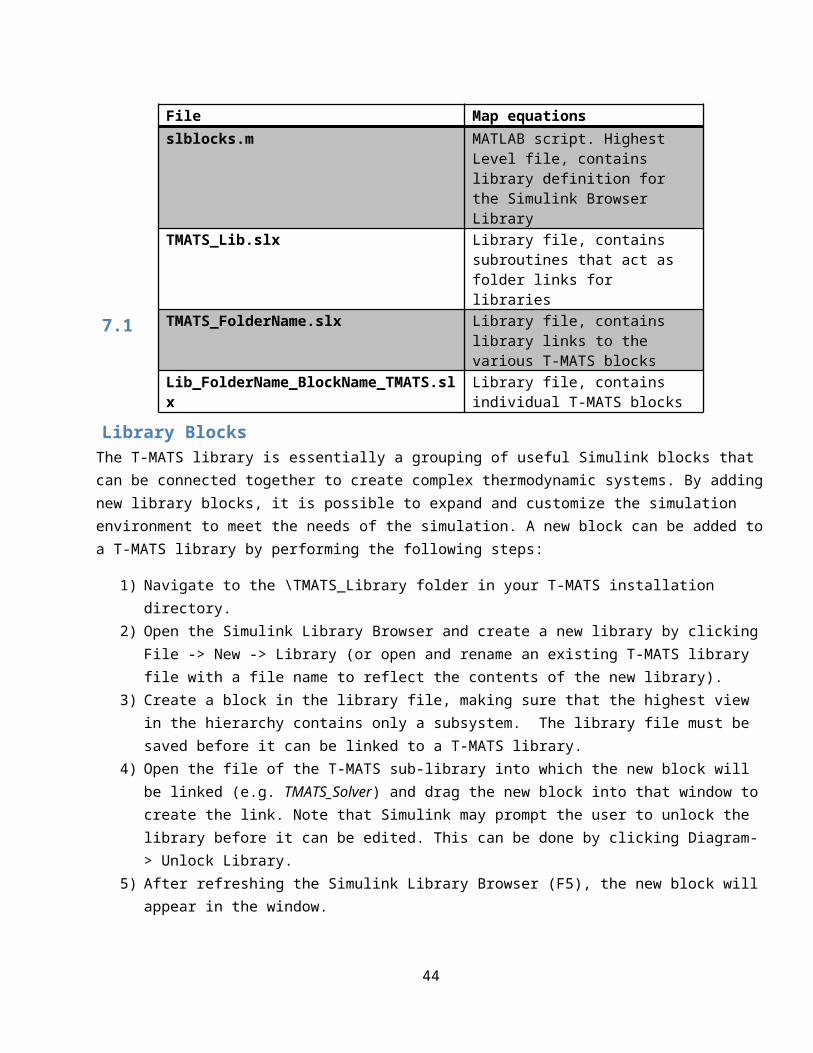
Figure 14. Gas turbine plant.

45

Ambient

Compressor

Shaft

Burner

Turbine

Duct

Nozzle

11.2.2 Plant Solver integration and plant inputs1) Create the solver

Place the TMATS: SS NR Solver w Jacobian Calc block in the model. Multiplex all dependent variables (component outputs color coded in green) and Ndot (from the shaft) and route the signal to the f(x) input of the solver block. De-multiplex the output of the solver block, X, and route each independent variable to one of the dark green inputs of the component blocks; one of the independent variables should be routed to the NMech input of the shaft block. In this example there are four independent variables and four dependent variables, as shown in Figure 15, where display blocks have been added to the solver input and output to aid in determining if the solver has converged to a solution.

2) Set up the solver parameters Once the signals have been connected, the solver mask parameters should be defined; these parameters include the initial conditions, the termination conditions, and other values that affect the accuracy of the solver. See the example for the values used for this model.

46

Figure 15. Steady-state solver setup.

47

3) Configure the solverOpen the simulation configuration window (Simulation -> Model Configuration Parameters on the Simulink menu bar) and select a fixed-step discrete solver, specifying the start and stop times as well as the fixed step size. (See the tutorial in Section 11.1 for more information on setting up the solver for simulation.)

4) Running the simulationOnce the engine model has been created and connected to the solver, the simulation can be run by pressing the run button located in the menu bar. After completing the run, the display blocks should be checked for convergence. It can be seen in Table 13 that the independent and dependent variables in example 2 are being driven to convergence (that is, the flow errors approach zero).

Table 13. Example 2 convergence outputs.

Independent variable Independent Request (value)

Dependent Variable Errors(dependent value)

W (system input) 101.2 pps Normalized flow error Nozzle 6.413e-06 N/AR-line (compressor) 1.955 N/A Normalized flow error compressor 6.379e-06 N/APRmap (turbine) 3.054 psia/psia Normalized flow error Turbine 4.884e-06 N/ANmech (shaft) 9980 rpm Ndot (shaft) 0.007742 rpm/sec

Because the steady-state gas turbine example requires definition of a large number of block parameters, the example was developed to utilize a setup script (the filename has the suffix “_setup_everything”). When run, this script creates a path to the SimSetup folder and runs all the files in that folder, which create the variable MWS in the workspace. This variable is a MATLAB data structure that contains many of the variables used in the example, which can be accessed with the syntax: MWS.Component.Variable (for example, MWS.HPC.s_Wc can be used to access the scalar for the Wc map in the HPC). When the simulation is run, Simulink will look for MWS in the MATLAB workspace and load the required variables. The example has been configured to automatically remove the temporary paths (created by the setup script) by running a cleanup script when the model file is closed.

48

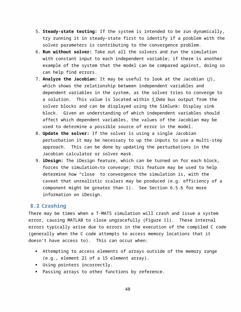
11.3 T-MATS example 3: Example_GasTurbine_DynAlthough it has the capability to solve for a steady-state condition, T-MATS is designed to ultimately be used in a dynamic simulation environment. This section will describe how to create a dynamic gas turbine simulation using T-MATS blocks and will also provide demonstration of various MATLAB practices the user may wish to utilize when developing a new simulation. This example is included in the examples section of T-MATS (GasTurbine_Dyn_Template.slx).

Before attempting to recreate the dynamic gas turbine simulation example, the user should read through the previous two examples, as certain topics covered in them will be skipped here. In particular, the description of how to structure the model assumes that the engine plant model has already been constructed, following the instructions presented in Section 11.2 for the steady-state gas turbine simulation.

11.3.1 General ArchitectureImplementing a dynamic solver in T-MATS requires that at least two separate loops be set up. This example uses an “inner” loop, which solves for convergence, and an “outer” loop, which steps through time. The “inner” loop includes the plant and the solver, and is where the independent variables are solved for from the dependent variables. The “outer” loop sets up the dynamic portion of the simulation and represents evolution of the system, which is converged at each time-step, over time. A hierarchical approach is required when creating such nested loops in Simulink (see Section 6.1 for more details).

11.3.1.1 Creating a Dynamic Simulation framework1) Set up the inner loop

Starting with the steady-state model described in the previous section, place a Simulink: While Iterator Subsystem in the model. Enter the subsystem and double-click the Simulink: While Iterator block to open the parameter window. Make the following changes: set the maximum number of iterations to -1, change the loop type to “do-while”, and check the box next to the “Show iteration number port” option.

2) Prepare the steady-state model for dynamic simulation Delete the default input and output ports in the Simulink: While Iterator Subsystem. Copy and paste the entire steady-state model (plant and solver blocks) into the subsystem. It may be helpful at this step to place the plant in its own subsystem within the while-iterator subsystem, as shown in Figure 16, where the low-level gas turbine components have been placed in the InnerLoopPlant subsystem.

3) Add the dynamic solver Replace the TMATS: SS NR Solver w JacobianCalc block with the TMATS: Iterative NR Solver w JacobianCalc block and connect the do_while_Condition output of the T-MATS solver to the cond input of the Simulink: While Iterator block, and the output of the Simulink: While Iterator block to the Iterations input of the T-MATS solver block, as shown in Figure 16.

4) Set up the solverIn the dynamic simulation, shaft speed is not one of the solver independent variables; reduce the order of the system by removing Ndot from the input to the solver block, and NMech from the output of the block, at the same time routing Ndot to the outer loop of the model and creating an input (for NMech) from the outer loop to the plant model. (A bus selector may be used for routing signals; see Section 11.3.4.1 for more information on this modification.)

49

Figure 16. Iterative NR Solver w JacobianCalc wiring.

50

5) Setup the outer loop Outside of the while iterator subsystem, route Ndot to the input of the TMATS: OuterLoop integrator block from the “Solver” sub-library (a bus selector may be used) and route the output of the integrator block to the NMech input of the plant (in the inner loop).To speed up the ability to modify the model when running multiple simulations, the environmental inputs (to the TMATS: Ambient block) and the fuel flow input (to the TMATS: Burner block), may similarly be routed from the outer loop to the inner loop. Bus creators may be used to combine these signals with NMech, as shown in Figure 17, to produce a cleaner-looking model.

6) Define the plant inputsEnvironmental inputs and fuel flow may be defined by connecting TMATS: Model Source blocks (from the “Solver” sub-library) to the respective inputs. The mask parameters for these blocks include a time vector and a vector that defines the values the signal takes at each time; the simulation profile can be defined through these inputs.

51

Figure 17. Dynamic gas turbine simple “outer” loop.

52

11.3.2 Adding control to the simulationThis section will describe how to add a simple feedback controller to the T-MATS simulation that uses shaft speed as the feedback signal.

1) Prepare the open-loop model for a controllerReplace the fuel flow TMATS: Model Source block with a TMATS: Model Source block for the shaft speed and place a TMATS: Simple PI controller block (from the “Effectors and Controls” sub-library) in the outer loop of the model

2) Connect the controllerWire Nmech, the output of the outer loop integrator block, to the Input_sensed input of the PI controller (this may require adding a Simulink: Zero-Order Hold block to sample Nmech). Also wire the output of the TMATS: Model Source block for shaft speed to the Input_dmd input of the PI controller, as shown in Figure 18. The output of the PI controller block should be wired to the fuel flow input of the burner block in the inner loop (i.e., inside the subsystem with the Simulink: While Iterator block).

3) Tune the controllerThe gains of the controller (defined in the mask parameters) may be tuned until the desired response is obtained. Note that although the PI controller may function adequately in a simple gas turbine, it does not represent a realistic gas turbine controller and will not have the ability to account for multi-variable constraints without significant modification.

53

Figure 18. Dynamic gas turbine with controller.

54

11.3.3 Plant interface with outer loop systemsIn a real system, engine effectors and internal states need to be accessed with control system hardware. The T-MATS package comes with generic controller interface blocks, such as the first-order sensor and actuator blocks in the “Effectors and Controls” sub-library, which may be used to simulate the dynamics introduced with added hardware. These blocks may be added to the “outer” loop of the model to increase simulation fidelity.

11.3.4 Advanced Simulation Structure and FormattingThe dynamic gas turbine example employs a few optional structural and formatting techniques that help to organize and partition the simulation. These options are useful when developing a complicated model or when several developers are collaborating to create the model. The techniques described in this section are based on MATLAB/Simulink blocks and are independent of the T-MATS package.

11.3.4.1 BussesBusses are a useful way to route signals through a Simulink model while keeping the diagram clean.

Creating Busses:1) Place a Simulink: Bus Creator block in the model. Any signal fed into that bus creator will be on the

bus and associated with the name of the wire fed into the bus creator. (Note that this is the only step required if a bus stays within a single model.)

2) The Bus Editor (found in the Edit menu) may be used to create bus elements. A bus that has been created in the Simulink diagram should also be created in the Bus Editor, being careful to organize the elements in the same order as they appear in the Simulink diagram.

3) After creating the bus, in the Bus Editor, select “Export to File” in the File menu of the editor. This saves the bus to a file that must be loaded before opening the Simulink model. (For example, the setup_everything.m script for the GasTurbine_Dyn_Template example loads all the necessary bus elements from the folder Bus)

4) To add any element to the bus later, these steps must be repeated (i.e., open the bus editor, add the new item, then save the item to a file.)

Using Busses:1) Bus elements may be routed off the bus through the use of the Simulink: Bus Selector block.

Simply wire the bus into the selector, and then use the dialog box to select which bus element(s) to output.

11.3.4.2 Model CallsModel calls may be used to incorporate external files into a Simulink model. This type of partitioning has three main advantages: it allows multiple users to work on the simulation at the same time (provided they don’t need the same file at the same time), it enables cleaner software version control, and it enables model reuse.

Setting up a model call requires placing a Simulink: Model block, from the “Ports and Subsystems” sub-library, in the model. Once the block has been placed, the file name of the model to be called should be specified in the dialog box opened by double-clicking the block. In the gas turbine example with the dynamics solver, calls were made to external plant and control models. The simulation may use Simulink: Model blocks with busses, which requires that the bus object creation method be followed.

55

Model Calls can also be used to simulate the plant in multiple simulation environments. For example, a steady–state simulation environment and a dynamic simulation environment could be created that both reference the same plant. This way, instead of having to modify two models to update the plant, a single file (containing the plant model) may be modified and these changes would be reflected in both simulation environments.

56

12 AcknowledgmentsThe authors would like to thank Alicia Zinnecker and Yuan Liu of N & R Engineering, and Jeffrey Csank of NASA Glenn Research Center for their work on T-MATS testing and for general technical advice. We would also like to thank Sanjay Garg at NASA Glenn Research Center for his support in the development of T-MATS, and the NASA Aviation Safety Program’s Vehicle Systems Safety Technologies (VSST) project for funding this work.

57

13 Appendix AMEX generation file:

/* T-MATS -- Burner_TMATS.c * % ************************************************************************* * % written by Jeffryes Chapman based on work by R. May and T. Lavelle * % NASA Glenn Research Center, Cleveland, OH * % February 27th, 2013 * % * % This file models the Burner Element for T-MATS simulation * % *************************************************************************/#define S_FUNCTION_NAME Burner_TMATS#define S_FUNCTION_LEVEL 2#include "simstruc.h"#include "functions_TMATS.h"#include "types_TMATS.h" #define LHV_p(S) ssGetSFcnParam(S,0)#define dPnormBurner_p(S) ssGetSFcnParam(S,1)#define Efficiency_p(S) ssGetSFcnParam(S,2)#define LHVEn_p(S) ssGetSFcnParam(S,3)#define hFuel_p(S) ssGetSFcnParam(S,4)#define NPARAMS 5 /* Forward declaration for Burner body of calcs */ extern void Burner_TMATS_body(real_T*, const real_T*, const BurnStruct*);

#define MDL_SET_WORK_WIDTHS /* Change to #undef to remove function */#if defined(MDL_SET_WORK_WIDTHS) && defined(MATLAB_MEX_FILE)/* Function: mdlSetWorkWidths =============================================== * Abstract: * Set up run-time parameters. */ static void mdlSetWorkWidths(SimStruct *S){ const char_T *rtParamNames[] = {"LHV", "DPnormBurner", "Eff", "LHVEn", "hFuel"}; ssRegAllTunableParamsAsRunTimeParams(S, rtParamNames);}#endif /* MDL_SET_WORK_WIDTHS */ static void mdlInitializeSizes(SimStruct *S){ int i; ssSetNumSFcnParams(S, NPARAMS); /* Number of expected parameters */ if (ssGetNumSFcnParams(S) != ssGetSFcnParamsCount(S)) { /* Return if number of expected != number of actual parameters */ return; }

58

Function parameter inputs.

Number of parameter inputs

C code function call definition

/* Set Block parameters tunable Note: Original version had all parameters set to non-tunable(?) */ for (i = 0; i < NPARAMS; i++) ssSetSFcnParamTunable(S, i, 1); ssSetNumContStates(S, 0); ssSetNumDiscStates(S, 0); if (!ssSetNumInputPorts(S, 1)) return; ssSetInputPortWidth(S, 0, 6); ssSetInputPortRequiredContiguous(S, 0, true); ssSetInputPortDirectFeedThrough(S, 0, 1); if (!ssSetNumOutputPorts(S, 1)) return; ssSetOutputPortWidth(S, 0, 6); ssSetNumSampleTimes(S, 1); ssSetNumRWork(S, 0); ssSetNumIWork(S, 0); ssSetNumPWork(S, 0); ssSetNumModes(S, 0); ssSetNumNonsampledZCs(S, 0); ssSetOptions(S, SS_OPTION_WORKS_WITH_CODE_REUSE | SS_OPTION_USE_TLC_WITH_ACCELERATOR); /* Register reserved identifiers to avoid name conflict */ if (ssRTWGenIsCodeGen(S) || ssGetSimMode(S)==SS_SIMMODE_EXTERNAL) { /* Register reserved identifier for OutputFcnSpec */ ssRegMdlInfo(S, "Burner_TMATS_body", MDL_INFO_ID_RESERVED, 0, 0, ssGetPath(S)); }} static void mdlInitializeSampleTimes(SimStruct *S){ ssSetSampleTime(S, 0, INHERITED_SAMPLE_TIME); ssSetOffsetTime(S, 0, 0.0); ssSetModelReferenceSampleTimeDefaultInheritance(S);} #define MDL_START#if defined(MDL_START)static void mdlStart(SimStruct *S){ }#endif static void mdlOutputs(SimStruct *S, int_T tid){ /* Input and output vectors */ const real_T *u = (const real_T*) ssGetInputPortSignal(S,0);

59

Number of inputs within the first inport

Number of inputs within the first outport

Begin C code for S-function here

real_T *y = (real_T *) ssGetOutputPortRealSignal(S,0); /* Block mask parameter struct */ BurnStruct burnPrms; burnPrms.LHV = *mxGetPr(LHV_p(S)); burnPrms.dPnormBurner = *mxGetPr(dPnormBurner_p(S)); burnPrms.Eff = *mxGetPr(Efficiency_p(S)); burnPrms.LHVEn = *mxGetPr(LHVEn_p(S)); burnPrms.hFuel = *mxGetPr(hFuel_p(S)); /* Perform core block calculations */ Burner_TMATS_body(y, u, &burnPrms);} static void mdlTerminate(SimStruct *S){} #ifdef MATLAB_MEX_FILE /* Is this file being compiled as a MEX-file? */#include "simulink.c" /* MEX-file interface mechanism */#else#include "cg_sfun.h" /* Code generation registration function */#endif/*==================*/

TLC generation file:%% File : Bleed_TMATS.tlc%%%% Description: %% Simulink Coder TLC Code Generation file for Bleed_TMATS%%%implements Bleed_TMATS "C" %% Function: BlockTypeSetup ===============================================%%%function BlockTypeSetup(block, system) void %% %% The Target Language must be C %if ::GenCPP==1 %<LibReportFatalError("This S-Function generated by the Legacy Code Tool must be only used with the C Target Language")> %endif %<LibAddToCommonIncludes("types_TMATS.h")> %<SLibAddToStaticSources("Bleed_TMATS_body.c")> %openfile forwardDecls extern void Bleed_TMATS_body(double *y, double *y1, const double *u, const double *BldInFlow, const BleedStruct* prm); BleedStruct bleedStruct; %closefile forwardDecls

60

Perform Core calculations

Perform Core calculations

%assign srcFile = LibGetModelDotCFile() %<LibSetSourceFileSection(srcFile, "Definitions", forwardDecls)> %endfunction %% Function: BlockInstanceSetup ===========================================%%%function BlockInstanceSetup(block, system) void %% %<LibBlockSetIsExpressionCompliant(block)>%endfunction %% Function: Outputs ======================================================%%%function Outputs(block, system) Output %% bleedStruct.WfracLen = %<LibBlockParameter(WfracLen,"","",0)>; bleedStruct.Wfrac = (double*)(%<LibBlockParameterBaseAddr(Wfrac)>); bleedStruct.IWork = &%<LibBlockIWork(Errors,"","",0)>; bleedStruct.BlkNm = "%<LibGetFormattedBlockPath(block)>"; %assign y_ptr = LibBlockOutputSignalAddr(0, "", "", 0) %assign y_dataType = LibBlockOutputSignalDataTypeName(0,"") %assign y1_ptr = LibBlockOutputSignalAddr(1, "", "", 0) %assign y1_dataType = LibBlockOutputSignalDataTypeName(1,"") %assign u_ptr = LibBlockInputSignalAddr(0, "", "", 0) %assign u_dataType = LibBlockInputSignalDataTypeName(0,"") %assign BldInFlow_ptr = LibBlockInputSignalAddr(1, "", "", 0) %assign BldInFlow_dataType = LibBlockInputSignalDataTypeName(1,"") %% Bleed_TMATS_body((%<y_dataType>*)%<y_ptr>,\ (%<y1_dataType>*)%<y1_ptr>,\ (%<u_dataType>*)%<u_ptr>,\ (%<BldInFlow_dataType>*)%<BldInFlow_ptr>,\ &bleedStruct); %%%endfunction %% [EOF]

Core calculation file:#include "types_TMATS.h"#include "constants_TMATS.h"#include "functions_TMATS.h"#include <math.h> #ifdef MATLAB_MEX_FILE#include "simstruc.h"#endif void Bleed_TMATS_body(double *y, double *y1, const double *u, const double *BldInFlow, const BleedStruct* prm){

61

Assign inputs and outputs

Inputs

double WIn = u[0]; /* Input Flow [pps] */ double htIn = u[1]; /* Input Enthalpy [BTU/lbm] */ double TtIn = u[2]; /* Temperature Input [degR] */ double PtIn = u[3]; /* Pressure [psia] */ double FARIn = u[4]; /* combusted Fuel to Air Ratio [frac] */ double BldInLen = u[5]; /* Length of Bleed Vector input */ /*--------Define Constants-------*/ double Wfin, htin, Test; double WOut, htOut, TtOut, PtOut, FAROut, WbldoutTotal; double Ws1,hts1,Tts1,Pts1,FARs1, Wfs1; double dHblds1, dHbldout, Wblds1, Wbldout, Wfblds1, Wfbldout; int Vtest; int i; /* define arrays for bleed outputs */ /* output bleeds */ double WbldOut[100]; double FARbldOut[100]; double PtbldOut[100]; double TtbldOut[100]; double htbldOut[100]; /* input bleeds */ double Wbld[100]; double FARbld[100]; double Ptbld[100]; double Ttbld[100]; double htbld[100]; /* Verify input bleed vector is a multiple of 5 */ Vtest = BldInLen/5; if(5*Vtest != BldInLen && *(prm->IWork+Er1)==0){ #ifdef MATLAB_MEX_FILE printf("Error in %s, one or more of the cooling flow input vector elements is missing(Vector form; 5x1: W,ht,Tt,Pt,FAR)\n",prm->BlkNm); #endif *(prm->IWork+Er1) = 1; } /* unpack BleedFlow vector */ for (i = 0; i < BldInLen/5; i++) { Wbld[i] = BldInFlow[5*i]; Ttbld[i] = BldInFlow[5*i+2]; Ptbld[i] = BldInFlow[5*i+3]; FARbld[i] = BldInFlow[5*i+4]; htbld[i] = t2hc(Ttbld[i],FARbld[i]); } /* Initialize cooling flow sum constants */ dHblds1 = 0; /* enthalpy * mass cooling flow rate at stage 1 */ Wblds1 = 0; /* total cooling flow at stage 1*/ Wfblds1 = 0; /* combusted fuel flow in cooling at stage */

62

Variable Definition

Core algorithms

/* calc station 1 bleed parameters */ for (i = 0; i < BldInLen/5; i++) { Wblds1 = Wblds1 + Wbld[i]; Wfblds1 = Wfblds1 + FARbld[i]*Wbld[i]*divby(1+FARbld[i]); dHblds1 = dHblds1 + htbld[i]*Wbld[i]; } /* calc station 1 flow parameters */ Ws1 = Wblds1 + WIn; Wfin = FARIn * WIn*divby(1+FARIn); Wfs1 = Wfblds1 + Wfin; FARs1 = Wfs1*divby(Ws1 - Wfs1); htin = t2hc(TtIn,FARIn); hts1 = (htin* WIn + dHblds1)*divby(Ws1); Tts1 = h2tc(hts1,FARs1); Pts1 = PtIn; htOut = hts1; TtOut = Tts1; PtOut = Pts1; FAROut = FARs1; WbldoutTotal = 0; for (i = 0; i < prm->WfracLen; i++) { WbldOut[i] = prm->Wfrac[i]*WIn; WbldoutTotal = WbldoutTotal +WbldOut[i]; } WOut = Ws1 - WbldoutTotal; Test = PtIn; /*------Assign output values------------*/ y[0] = WOut; /* Outlet Total Flow [pps] */ y[1] = htOut; /* Outlet Enthalpy [BTU/lbm]*/ y[2] = TtOut; /* Outlet Temperature [degR] */ y[3] = PtOut; /* Outlet Pressure [psia] */ y[4] = FAROut; /* Outlet Fuel to Air Ratio [NA] */ y[5] = Test; /*------Assign output values port2------------*/ /* fractional bleed, typically used for turbine cooling flow */ for (i = 0; i < prm->WfracLen; i++) { *y1++ = WbldOut[i]; *y1++ = htOut; *y1++ = TtOut; *y1++ = PtOut; *y1++ = FAROut; } }

63

Outputs

64