International Conference on Mathematics and Computational Methods Applied to Nuclear Science & Engineering (M&C 2013)Sun Valley, Idaho, USA, May 5-9, 2013, on CD-ROM, American Nuclear Society, LaGrange Park, IL (2013)

RAVEN AS A TOOL FOR DYNAMIC PROBABILISTIC RISKASSESSMENT: SOFTWARE OVERVIEW

A. Alfonsi, C. Rabiti, D. Mandelli, J.J. Cogliati, R.A. KinoshitaIdaho National Laboratory

2525 Fremont Avenue, Idaho Falls, ID 83415{andrea.alfonsi, cristian.rabiti, diego.mandelli, joshua.cogliati, robert.kinoshita}@inl.gov

ABSTRACT

RAVEN is a software tool under development at the Idaho National Laboratory (INL) that acts as thecontrol logic driver and post-processing tool for the newly developed Thermo-Hydraylic code RELAP-7. The scope of this paper is to show the software structure of RAVEN and its utilization in connectionwith RELAP-7. A short overview of the mathematical framework behind the code is presented alongwith its main capabilities such as on-line controlling/monitoring and Monte-Carlo sampling. A demo ofa Station Black Out PRA analysis of a simplified Pressurized Water Reactor (PWR) model is shown inorder to demonstrate the Monte-Carlo and clustering capabilities.

Key Words: Reactor Simulation, Probabilistic Risk Assessment, Dynamic PRA, Monte-Carlo, RELAP-7

1. INTRODUCTION

RAVEN (Reactor Analysis and Virtual control ENviroment) [1,2] is a software tool that acts as the con-trol logic driver for the newly developed Thermo-Hydraylic code RELAP-7. The goal of this paper is tohighlight the software structure of the code and its utilization in conjunction with RELAP-7. RAVEN isa multi-purpose Probabilistic Risk Assement (PRA) software framework that allows dispatching differentfunctionalities. It is designed to derive and actuate the control logic required to simulate the plant controlsystem and operator actions (guided procedures) and to perform both Monte-Carlo sampling of random dis-tributed events and event tree based analysis. In order to facilitate the input/output handling, a GraphicalUser Interface (GUI) and a post-processing data mining module, based on dimensionality and cardinalityreduction, are available. This paper wants to provide an overview of the software, highlighting the mathe-matical framework from which its structure is derived and showing a demo of a Station Black Out (SBO)analysis of a simplified Pressurized Water Reactor (PWR) model.

2. MATHEMATICAL FRAMEWORK

In this section the mathematical framework is briefly described by analyzing the set of the equations neededto model the control system in a nuclear power plant.

2.1. Plant and Control System Model

The first step is the derivation of the mathematical model representing, at a high level of abstraction, boththe plant and the control system models. In this respect, let be θ(t) a vector describing the plant status in thephase space; the dynamic of both plant and control system can be summarized by the following equation:

∂θ

∂t= H(θ(t), t) (1)

A. Alfonsi, C. Rabiti, D. Mandelli, J.J. Cogliati, R.A. Kinoshita

In the above equation we have assumed the time differentiability in the phase space. This is generally notrequired and it is used here for compactness of notation. Now an arbitrary decomposition of the phase spaceis performed:

θ =

(x

v

)(2)

The decomposition is made in such a way that x represents the unknowns solved by RELAP-7, while v arethe variables directly controlled by the control system (i.e., RAVEN). Equation 1 can now be rewritten asfollows:

∂x

∂t= F (x, v, t)

∂v

∂t= V (x, v, t)

(3)

As a next step, it is possible to note that the function V (x, v, t) representing the control system, does notdepend on the knowledge of the complete status of the system but on a restricted subset that we call controlvariables C:

∂x

∂t= F (x, v, t)

C = G(x, t)∂v

∂t= V (x, v, t)

(4)

2.2. Operator Splitting Approach

The system of equations in Eq. 4 is fully coupled and in the past it has always been solved with an operatorsplitting approach. The reasons for this choice are several:

• Control system reacts with an intrinsic delay

• The reaction of the control system might move the system between two different discrete states andtherefore numerical errors will be always of first order unless the discontinuity is treated explicitly.

RAVEN as well is using this approach to solve Eq. 4 which it becomes:∂x

∂t= F (x, vti−1, t)

C = G(x, t)∂v

∂t= V (x, vti−1, t)

(5)

2.3. The auxiliary plant and component status variables

So far it has been assumed that all information needed is contained in x and v. Even if this informationis sufficient for the calculation of the system status in every point in time, it is not a practical and efficientway to implement the control system. In order to facilitate the implementation of the control logic, a systemof auxiliary variables has been introduced . The auxiliary variables are those that in statistical analysis areartificially added to non-Markovian systems into the space phase to obtain back a Markovian behavior, sothat only the information contained in the previous time step is needed to determine the future status of thesystem. These variables can be classified into two types:

2/15

RAVEN as a tool for Dynamic Probabilistic Risk Assessment: Software Overview

• Global status auxiliary control variables (e.g., SCRAM status, time at which scram event begins, timeat which hot shut down event begins)

• Component status auxiliary variables (e.g., correct operating status, time from abnormal event)

Thus, the introduction of the auxiliary system into the mathematical framework leads to the following for-mulation of the Eq. 5:

∂x

∂t= F (x, vti−1, t)

C = G(x, t)∂a

∂t= A(x, C, a, vti−1, t)

∂v

∂t= V (x, vti−1, t)

(6)

3. RELAP-7 AND MOOSE

MOOSE [3] is a computer simulation framework, developed at Idaho National Laboratory (INL), that sim-plifies the process for predicting the behavior of complex systems and developing non-linear, multi-physicssimulation tools. As opposed to traditional data-flow oriented computational frameworks, MOOSE is basedon the mathematical principle of Jacobian-Free Newton-Krylov (JFNK) solution methods. Utilizing themathematical structure present in JFNK, physics are modularized into Kernels allowing for rapid produc-tion of new simulation tools. In addition, systems are solved fully coupled and fully implicit by employingphysics based preconditioning which allows for great flexibility even with large variance in time scales.Other than providing the algorithms for the solution of the differential equation, MOOSE also provides allthe manipulation tools for the C++ classes containing the solution vector. This framework has been used toconstruct and develop the Thermo-Hydraulic code RELAP-7, giving an enormous flexibility in the couplingprocedure with RAVEN.

RELAP-7 is the next generation nuclear reactor system safety analysis. It will become the main reactorsystems simulation toolkit for RISMC (Risk Informed Safety Margin Characterization) [4] project andthe next generation tool in the RELAP reactor safety/systems analysis application series (the replacementfor RELAP5). The key to the success of RELAP-7 is the simultaneous advancement of physical models,numerical methods, and software design while maintaining a solid user perspective. Physical models includeboth PDEs (Partial Differential Equations), ODEs (Ordinary Differential Equations) and experimental basedclosure models. RELAP-7 will eventually utilize well posed governing equations for multiphase flow, whichcan be strictly verified. RELAP-7 uses modern numerical methods which allow implicit time integration,higher order schemes in both time and space and strongly coupled multi-physics simulations. RELAP-7 isthe solver for the plant system except for the control system. From the mathematical formulation presentedSection 2, RELAP-7 solves ∂x

∂t = F (x, vti−1, t).

4. RAVEN

RAVEN has been developed in a high modular and pluggable way in order to enable easy integration ofdifferent programming languages (i.e., C++, Python) and coupling with other applications including theones based on MOOSE. The code consists of four modules:

3/15

A. Alfonsi, C. Rabiti, D. Mandelli, J.J. Cogliati, R.A. Kinoshita

!

!

!

!

!

!

MOOSE%

%RELAP'7!! !!" = !!!! , !!!!! , !!!! = ! !(!, !)!

RAVEN!(RELAP'7!Interface)!

!

!! !

RAVEN!(Control!Logic)!

!!!" = !!!!, !!!!! , !!!

!! ! !!! !

!!! !

Figure 1: Control System Software Layout.

• RAVEN/RELAP-7 interface (see Section 4.1)

• Python Control Logic (see Section 4.2)

• Python Calculation Driver (see Section 4.3)

• Graphical User Interface (see Section 4.4)

4.1. RAVEN/RELAP-7 interface

The RAVEN/RELAP-7 interface, coded in C++, is the container of all the tools needed to interact withRELAP-7/MOOSE. It has been designed in order to be general and pluggable with different solvers si-multaneously in order to allow an easier and faster development of the control logic/PRA capabilities formulti-physics applications. The interface provides all the capabilities to control, monitor, and process theparameters/quantities in order to drive the RELAP-7/MOOSE calculation. In addition, it contains the toolsto communicate to the MOOSE input parser whose information, i.e. input syntax, must be received as inputin order to run a RAVEN calculation. So far, the input file includes four main sections.:

• RavenMonitored class;

• RavenControlled class;

• RavenAuxiliary class;

• RavenDistributions class.

The RavenMonitored class provides the connection with the calculation framework in order to retrieve thepost-processed quantities from the simulation (e.g., average fuel temperature, average fluid pressure in acomponent). The typical input structure for a Monitored parameter in RAVEN is as following:

[Monitored][./ MaxTempCladCH1]

component name = CH1

4/15

RAVEN as a tool for Dynamic Probabilistic Risk Assessment: Software Overview

operator = NodalMaxValuepath = CLAD:TEMPERATUREdata type = double

[../][./ MaxTempCladCH2]

component name = CH2operator = NodalMaxValuepath = CLAD:TEMPERATUREdata type = double

[../]...

[]

Within the block identified by the keyword Monitored, the user can specify the monitored quantities thatneed to be processed during the calculation. Each monitored variable is identified through a Raven Alias(i.e., MaxTempCladCH1), the name that is used in the control logic Python input in order to refer to theparameter contained in the simulation. The user has to provide the following information in order to build amonitored variable:

• component name, the name of the RELAP-7 component that contains the variable the code must acton;

• operator, the post-processor operation that must be performed on the variable;

• path, the variable name and its location within the calculation framework (RELAP-7/MOOSE vari-able name);

• data type, data type (i.e., double, float, int, boolean).

RAVEN can use all the post-processor operators that are available in MOOSE (e.g., ElementAverageValue,NodalMaxValue, etc.). Depending on which component it’s acting on, some operations may be disabled (forexample, ElementAverageValue is not available in 0-D components).

The RavenControlled class provides the link between RAVEN and RELAP-7/MOOSE in order to retrieveand/or change properties within the simulation (e.g., fuel thermal conductivity, pump mass flow). The typicalinput structure for a controlled parameter in RAVEN is as follows:

[ Controlled ]control logic input = control logic input file name[./ power fraction CH1]

property name = FUEL:power fractiondata type = doublecomponent name = CH1

[../][./ power fraction CH2]

property name = FUEL:power fractiondata type = doublecomponent name = CH2

[../]...

[]

5/15

A. Alfonsi, C. Rabiti, D. Mandelli, J.J. Cogliati, R.A. Kinoshita

Within the block identified by the keyword Controlled, the user can specify the properties that, during thecalculation, will be controlled through the Python control logic. The name and path of the control logicinput file are provided by the parameter control logic input (not specifying the ”.py” extension). Eachcontrolled variable is identified through a Raven Alias (e.g., power fraction CH1): the name that is used inthe control logic Python input in order to refer to the parameter contained in the simulation. The user hasto provide different information in order to build a controlled variable:

• component name, the name of the RELAP-7 component that contains the variable the code must acton;

• property name, the variable name and its location within the calculation framework (RELAP-7/MOOSEvariable name);

• data type, data type (i.e., double, float, int, boolean).

Through this class, RAVEN is able to retrieve property values and, in case of changes, push the new valuesback into the simulation.

The RavenAuxiliary class is the container of auxiliary variables. The Raven Auxiliary system is not con-nected with RELAP-7/MOOSE environment. The typical input structure for a auxiliary parameter inRAVEN is as follows:

[RavenAuxiliary][./ scram start time ]

data type = doubleinitial value = 61.0

[../][./ CladDamaged]

data type = boolinitial value = False

[../]...

[]

Each auxiliary variable is identified through a Raven Alias (e.g., CladDamaged): the name that is used inthe control logic Python input in order to refer to the parameter contained in the RAVEN interface. Theuser has to provide different information in order to build a auxiliary variable:

• initial value, initialization value;

• data type, data type (i.e., double, float, int, bool).

As previously mentioned, these variables are needed to ensure that system remains Markovian, so that onlythe previous time step information are necessary to determine the future status of the plant.

The RavenDistributions class contains the algorithms, structures and interfaces for several predefined proba-bility distributions. It is only available in the Python control logic, since it is not needed a direct interactionwith RAVEN/RELAP-7/MOOSE environment. The user can actually choose among nine different types of

6/15

RAVEN as a tool for Dynamic Probabilistic Risk Assessment: Software Overview

distribution (e.g., Normal, Triangular, Uniform, Exponential); each of them, in order to be initialized, re-quires a different set of parameters depending on the type of distribution. An an example, the followinginput create a Normal and a Triangular distribution:

[ Distributions ][./ ExampleNormalDis]

type = NormalDistributionmu = 1sigma = 0.01xMax = 0.8xMin = 0

[../][./ ExampleTriangularDis]

type = TriangularDistributionxMin = 1255.3722xPeak = 1477.59xMax = 1699.8167

[../]...

[]

The class RavenDistributions is the base of the Monte-Carlo and Dynamic Event Tree capabilities presentin RAVEN.

4.2. Python Control Logic

The control logic module is used to drive a RAVEN/RELAP-7 calculation. Up to now it is implemented bythe user via Python scripting. The reason of this choice is to try to preserve generality of the approach inthe initial phases of the project so that further specialization is possible and inexpensive. The form throughwhich the RAVEN variables can be called is the following:

• Auxiliary.RavenAlias;

• Controlled.RavenAlias;

• Monitored.RavenAlias.

Regarding the RavenDistributions mentioned in Section 4.1, they are also available for the control logic in asimilar form to the other variable (distributions.RavenAlias(allowable list of arguments) ). The implemen-tation of the control logic via Python is rater convenient and flexible. The user only needs to know fewPython syntax rules in order to build an input. Although this extreme simplicity, it will be part of the GUItask to automatize the construction of the control logic scripting in order to minimize user effort.A small example of a control logic input is reported below: the thermal conductivity of the gap (thermal-ConductGap) is set equal to the thermal conductivity of the fuel when the fuel temperature (averageFuel-Temperature) is greater than 910 K.

import sysdef control function (monitored, controlled , auxiliary ):

if monitored.averageFuelTemperature > 910:controlled . thermalConductGap = controlled . thermalConductFuel

return

7/15

A. Alfonsi, C. Rabiti, D. Mandelli, J.J. Cogliati, R.A. Kinoshita

Figure 2: RAVEN Calculation Flow - Initialization.

8/15

RAVEN as a tool for Dynamic Probabilistic Risk Assessment: Software Overview

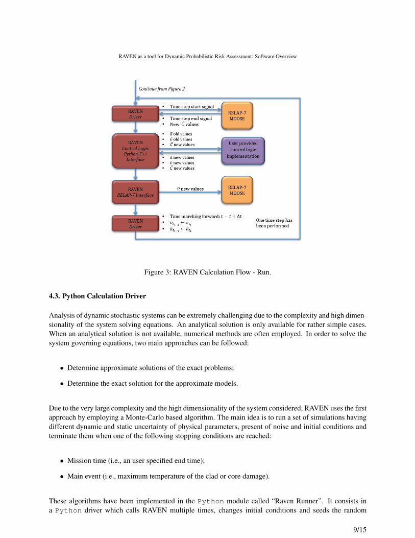
Figure 3: RAVEN Calculation Flow - Run.

4.3. Python Calculation Driver

Analysis of dynamic stochastic systems can be extremely challenging due to the complexity and high dimen-sionality of the system solving equations. An analytical solution is only available for rather simple cases.When an analytical solution is not available, numerical methods are often employed. In order to solve thesystem governing equations, two main approaches can be followed:

• Determine approximate solutions of the exact problems;

• Determine the exact solution for the approximate models.

Due to the very large complexity and the high dimensionality of the system considered, RAVEN uses the firstapproach by employing a Monte-Carlo based algorithm. The main idea is to run a set of simulations havingdifferent dynamic and static uncertainty of physical parameters, present of noise and initial conditions andterminate them when one of the following stopping conditions are reached:

• Mission time (i.e., an user specified end time);

• Main event (i.e., maximum temperature of the clad or core damage).

These algorithms have been implemented in the Python module called “Raven Runner”. It consists ina Python driver which calls RAVEN multiple times, changes initial conditions and seeds the random

9/15

A. Alfonsi, C. Rabiti, D. Mandelli, J.J. Cogliati, R.A. Kinoshita

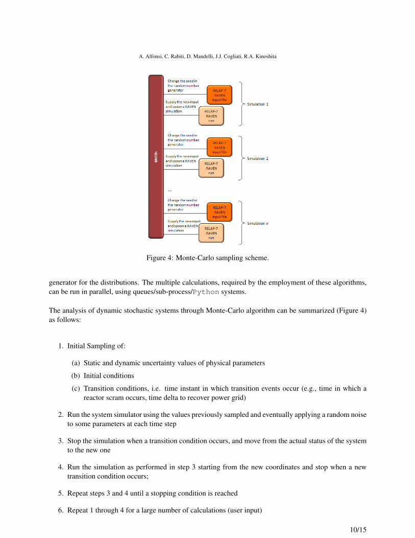
Figure 4: Monte-Carlo sampling scheme.

generator for the distributions. The multiple calculations, required by the employment of these algorithms,can be run in parallel, using queues/sub-process/Python systems.

The analysis of dynamic stochastic systems through Monte-Carlo algorithm can be summarized (Figure 4)as follows:

1. Initial Sampling of:

(a) Static and dynamic uncertainty values of physical parameters

(b) Initial conditions

(c) Transition conditions, i.e. time instant in which transition events occur (e.g., time in which areactor scram occurs, time delta to recover power grid)

2. Run the system simulator using the values previously sampled and eventually applying a random noiseto some parameters at each time step

3. Stop the simulation when a transition condition occurs, and move from the actual status of the systemto the new one

4. Run the simulation as performed in step 3 starting from the new coordinates and stop when a newtransition condition occurs;

5. Repeat steps 3 and 4 until a stopping condition is reached

6. Repeat 1 through 4 for a large number of calculations (user input)

10/15

RAVEN as a tool for Dynamic Probabilistic Risk Assessment: Software Overview

Figure 5: Input/plan Visualization GUI Window.

Figure 4 shows a scheme of the interaction between the code and the RAVEN runner in case of Monte-Carlocalculations. The runner basically perform a different seeding of the random number generator and interact,through RAVEN, with the Python control logic input in order to sample the variables specified by the user.

4.4. Graphical User Interface

As previously mentioned, a Graphical User Interface (GUI) is not required to run RAVEN, but it representsan added value to the whole code. The GUI is compatible with all the capabilities actually present in RAVEN(control logic, Monte-Carlo, etc.). Its development is performed using QtPy, which is a Python interfacefor a C++ based library (C++) for GUI implementation. The GUI is based on a software named Peacock,which is a GUI interface for MOOSE based application and, in its base implementation, is only able toassist the user in the creation of the input. In order to make it fit all the RAVEN needs, the GUI has beenspecialized and it is in continuous evolution.

5. SOFTWARE LAYOUT AND CALCULATION FLOW

Figures 2 and 3 show the calculation flow employed by RAVEN/RELAP-7/MOOSE software. A typicalRAVEN calculation can be summarized in the following logic steps:

1. Perform Initialization

2. RELAP-7/MOOSE updates the information contained in each component class with the actual solu-tion x

3. RAVEN requests MOOSE to perform the post-processing manipulation in order to construct C

11/15

A. Alfonsi, C. Rabiti, D. Mandelli, J.J. Cogliati, R.A. Kinoshita

Figure 6: PWR model scheme.

4. Equation ∂v∂t = V (x, vti−1, t) is solved and the set of control parameters for the next time step vti is

determined

5. RAVEN asks RELAP-7/MOOSE to compute the solution x for the following time step

6. Repeat from 2 to 5 until the end of the calculation or an exit condition is reached (e.g., clad failure)

6. DEMO FOR A PWR PRA ANALYSIS

In order to show the capabilities of RAVEN coupled with RELAP-7/MOOSE, a simplified PWR PRA anal-ysis has been employed. Figure 6 shows the scheme of the PWR model. The reactor vessel model consistsof the Down-comers, the Lower Plenum, the Reactor Core Model and the Upper Plenum. Core channels(flow channels with heat structure attached to each of them) were used to describe the reactor core. The coremodel consists of three parallel core channels and one bypass flow channel. There are two primary loops,i.e., loop A and loop B. Each loop consists of the Hot Leg, a Heat Exchanger and its secondary side pipes,the Cold Leg and a primary Pump. A Pressurizer is attached to the Loop A piping system to control thesystem pressure. A Time Dependent Volume (pressure boundary conditions) component is used to representthe Pressurizer. Since the RELAP-7 code does not have the two-phase flow capability yet, single-phasecounter-current heat exchanger models are implemented to mimic the function of steam generators in orderto transfer heat from the primary to the secondary. In order to perform a PRA analysis on this simplifiedmodel, it has been necessary to control unconventional parameters (i.e. inlet/outlet friction factors), sinceRELAP-7 still has limitations for the component controllable parameters and models. In the followingparagraph, the PRA station black out sequence of events is reported.

6.1. Station Black Out (SBO) analysis

The Probabilist Risk Assessment analysis has been performed simulating a Station Black Out accident,making Monte-Carlo samplings on the recovery time of the diesel generators t1 (delta time from reactorscram signal) and the clad failure temperature TCf . Two sets of Monte-Carlo calculations have been run:

• 400 runs, randomizing t1 (Normal distribution, mu = 120 s, sigma = 20 s) and TCf (Triangulardistribution, xPeak = 1477.59 K, xMin = 1255.37 K, xMax = 1699.82 K)

12/15

RAVEN as a tool for Dynamic Probabilistic Risk Assessment: Software Overview

• 400 runs, randomizing only t1

The SBO transient is based on the following sequence of events (starting from a steady-state operationalcondition of the Nuclear Power Plant [5]):

• 60.0 seconds, transient begins

• 61.0 seconds, loss of power grid and immediate shutdown of the reactor(scram):

– Pump coast-down;

– Decay heat power;

– Diesel Generators and residual heat removal system (RHRS) not available.

• t1, recovery of the diesel generators

• t2, end of transient either for clad failure or 300 seconds of simulation (PRA success)

Since the scope of this demo is to show the capabilities contained in RAVEN and RELAP-7 capabilities arenot optimized for long simulation times, the transient has been accelerated in order to simulate a maximumof 300 seconds. In the following paragraph, the simulations results are shown and explained.

6.2. Results

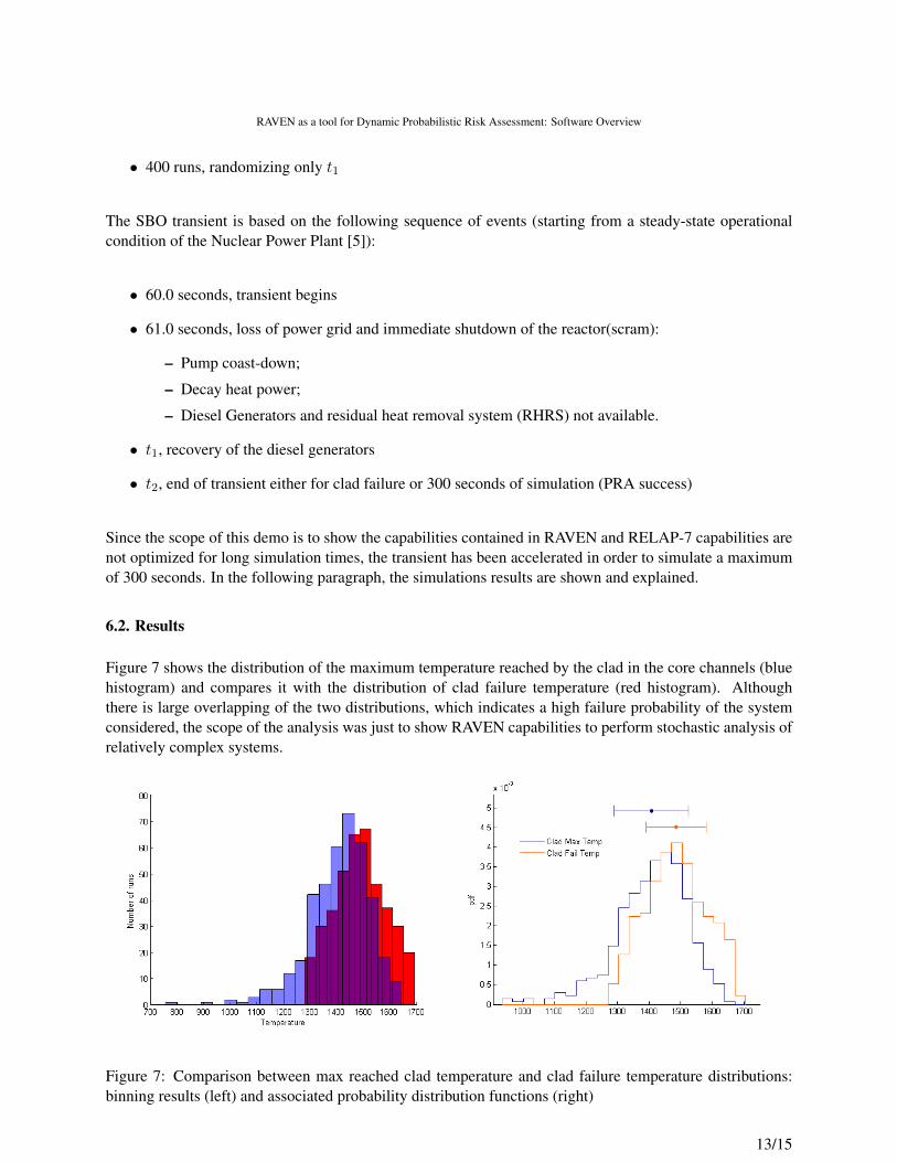
Figure 7 shows the distribution of the maximum temperature reached by the clad in the core channels (bluehistogram) and compares it with the distribution of clad failure temperature (red histogram). Althoughthere is large overlapping of the two distributions, which indicates a high failure probability of the systemconsidered, the scope of the analysis was just to show RAVEN capabilities to perform stochastic analysis ofrelatively complex systems.

Figure 7: Comparison between max reached clad temperature and clad failure temperature distributions:binning results (left) and associated probability distribution functions (right)

13/15

A. Alfonsi, C. Rabiti, D. Mandelli, J.J. Cogliati, R.A. Kinoshita

Figure 8: Limit Surface for the SBO analysis of a simplified PWR model

In addition, Fig. 8 shows the limit surface, i.e. the boundaries between system failure (red points) andsystem success (green points), obtained by the 400 Monte-Carlo simulations. Since only two uncertainparameters have been considered (i.e., DG recovery time and clad fail temperature), this boundary lies in a2-dimensional space. The slope of the limit surface pictured in Fig. 8 also shows, in this particular demo,how the DG recovery time has a greater impact on the system dynamics then the clad failure temperature.

It has also been performed a new set of 400 Monte-Carlo simulations in which, now, the clad failure tem-perature is fixed at a predefined value TFail = 1477.59 (i.e., there is no triangular distribution associated toit). As expected, the probability of core damage was slightly different among thee two set of simulations.This fact shows how modeling of uncertainties can impact risk evaluation.

7. CONCLUSIONS

In this paper it has been presented RAVEN as a tool to perform dynamic PRA through Monte-Carlo sam-pling. In particular, the software structure and all the components that are involved in the computation havebeen presented, including system simulator (i.e., RELAP-7) and the control logic, characterized by monitorsystem dynamics and on-line control of selected parameters. An example of PRA analysis has been alsopresented for a SBO-like case for a simplified PWR loop. The description of the implementation for suchcase demonstrates how the flexibility of the software framework provides the basic tools to perform Dy-namic PRA, uncertainty quantification and plant control. Next capabilities, to be implemented to RAVENand that are currently under development, include dynamic event tree generation [6], adaptive sampling [7]and more advanced data mining algorithms [8].

REFERENCES

[1] C. Rabiti, A. Alfonsi, J. Cogliati, D. Mandelli, and R. Kinoshita, “Reactor analysis and virtual controlenvironment (raven) fy12 report,” Tech. Rep. INL/EXT-12-27351, Idaho National Laboratory (INL),2012.

14/15

RAVEN as a tool for Dynamic Probabilistic Risk Assessment: Software Overview

[2] C. Rabiti, A. Alfonsi, D. Mandelli, J. Cogliati, and R. Martineau, “Raven as control logic and proba-bilistic risk assessment driver for relap-7,” in Proceeding of American Nuclear Society (ANS), San Diego(CA), vol. 107, pp. 333–335, 2012.

[3] D. Gaston, G. Hansen, S. Kadioglu, D. A. Knoll, C. Newman, H. Park, C. Permann, and W. Tai-tano, “Parallel multiphysics algorithms and software for computational nuclear engineering,” Journal ofPhysics: Conference Series, vol. 180, no. 1, p. 012012, 2009.

[4] D. Mandelli and C. Smith, “Integrating safety assessment methods using the risk informed safety mar-gins characterization (rismc) approach,” in Proceeding of American Nuclear Society (ANS), San Diego(CA), vol. 107, pp. 883–885, 2012.

[5] D. Anders, R. Berry, D. Gaston, R. Martineau, J. Peterson, H. Zhang, H. Zhao, and L. Zou, “Relap-7level 2 milestone report: Demonstration of a steady state single phase pwr simulation with relap-7,”Tech. Rep. INL/EXT-12-25924, Idaho National Laboratory (INL), 2012.

[6] A. Hakobyan, T. Aldemir, R. Denning, S. Dunagan, D. Kunsman, B. Rutt, and U. Catalyurek, “Dynamicgeneration of accident progression event trees,” Nuclear Engineering and Design, vol. 238, no. 12,pp. 3457 – 3467, 2008.

[7] D. Mandelli and C. Smith, “Adaptive sampling using support vector machines,” in Proceeding of Amer-ican Nuclear Society (ANS), San Diego (CA), vol. 107, pp. 736–738, 2012.

[8] D. Mandelli, A. Yilmaz, and T. Aldemir, “Scenario analysis and pra: Overview and lessons learned,” inProceedings of European Safety and Reliability Conference (ESREL 2011), Troyes (France), 2011.

15/15