Rational Transparency Choicein Financial Market Equilibrium∗

Marc-Andreas Muendler¶

University of California, San Diego and CESifo

December 5, 2005

AbstractAdd a stage of signal acquisition to a canonical model of portfolio choice.Under fully revealing asset price, investors’ information demand reflectstheir choice of transparency. In reducing uncertainty, financial trans-parency raises expected asset price and thus benefits holders of the riskyasset. At a natural transparency limit, however, investors pay to inhibitfurther disclosure in order to forestall the erosion of the asset’s expectedexcess return. The natural transparency limit varies with the portfolioposition. There is a dominant investor with a risky asset endowmentmodestly above market average who single-handedly determines trans-parency in equilibrium. The dominant investor strictly improves welfarefor investors with similar endowments but strictly reduces welfare for oth-ers when acquiring signals beyond their natural transparency limits. Thewelfare consequences of financial transparency are thus intricately linkedto the wealth distribution.

Keywords: Information acquisition; rational expectations equilibrium;fully revealing asset price; financial transparency; disclosure; gamma dis-tributed asset returns; Poisson distributed signals

JEL Classification: JEL D81, D83, G14

∗I thank Joel Sobel, Mark Machina, Ross Starr, Maury Obstfeld, Bob Anderson, DanMcFadden, Sven Rady, David Romer, Andy Rose, Tom Rothenberg, Chris Shannon and AchimWambach for insightful remarks. Seminar participants at University of Munich, City UniversityBusiness School London, George Washington University, Deutsche Bundesbank, Universityof California San Diego and at ESEM 2002 Venice made helpful suggestions. This papersubstantially extends a previously circulated version entitled “Another look at informationacquisition under fully revealing asset prices.”

¶muendler@ucsd.edu (econ.ucsd.edu/muendler). University of California San Diego, Dept.of Economics #0508, 9500 Gilman Dr., La Jolla, CA 92093-0508, USA

1

Financial transparency is widely regarded as a cornerstone of well-functioningcapital markets and a remedy to financial distress. What is the welfare effectof financial transparency? This paper pays close attention to the importance ofheterogeneous portfolios and financial market conditions for the economic valueof transparency. The paper shows that there is a natural transparency limit atwhich rational investors pay to inhibit disclosure. The natural transparency limitvaries with initial portfolio holdings.

A literature on learning and experimentation analyzes incentives for infor-mation acquisition and the public-goods character of information, but frequentlytreats markets in abstract terms and disregards equilibrium price effects of trans-parency. Many models of financial information, on the other hand, consider sig-nal receipt as exogenous to investors. The framework of this paper permits ananalysis of the utility value of financial transparency based on first principles.To determine the economic value of financial transparency, the paper examinesfully revealing asset price. Under fully revealing price, the choice of individualinformation becomes a choice of public transparency. Finitely many rational in-vestors have well-defined signal demands which, in turn, capture the marginalutility benefits and costs of transparency.

Natural transparency limits arise because, as information removes risk, itraises expected asset price and diminishes an asset’s expected excess return. Atan investor’s transparency limit, the utility loss from diminished excess returnsoutweighs information benefits. To take an example, risk averse investors arecompensated for default risk with returns that exceed the expected losses un-der default. More information strictly diminishes this excess return. At thetransparency limit, rational lenders reject further information to keep the excessreturn. Prior to investors’ natural transparency limits, financial information is apublic good.

An investor’s natural transparency limit crucially depends on initial port-folio holdings. When initial portfolio positions are heterogeneous, a dominantinvestor with an endowment close to market average emerges and dictates thetransparency outcome.1 Transparency makes the asset safer and thus raises theexpected asset price. A higher expected asset price benefits the dominant in-vestor most, who holds an asset endowment modestly above market average.Investors with smaller asset holdings experience only a smaller revaluation effectfrom more transparency, and investors with larger holdings suffer more from thehigher expected variance of their endowment value because signal realizationsmay be favorable or unfavorable. The dominant investor acquires information toa degree that makes investors with smaller or larger initial asset holdings strictly

1This heterogeneity in endowments generalizes Muendler (2005) and stresses the importanceof the wealth distribution for informational welfare.

2

worse off if the acquired number of signals exceeds those investors’ transparencylimits. As a consequence, additional information results in an unambiguousPareto improvement only if investors are sufficiently homogeneous.

Information and transparency are matters of degree. Beyond binary infor-mation acquisition as in Grossman and Stiglitz (1980) or Diamond (1985), thepresent paper gives investors a choice of a number of signals in the spirit of ex-perimentation. The present setup draws on Raiffa and Schlaifer (1961) whoseconjugate-prior decision model provides a natural extension of the canonical port-folio choice model and gives rise to a law of demand for financial information—similar to the experimentation paradigm of repeated sampling (Moscarini andSmith 2001) but for risk averse, not risk neutral, agents. Most important, thisapproach allows rational investors to account for the equilibrium price impact oftransparency. Demand for transparency is strong if many risky assets are in themarket, or if investors are highly risk averse, or if the expected mean-varianceratio of the asset return is relatively low so that uncertainty matters stronglycompared to expected returns.

Recent financial-market or general-equilibrium models address transparencybut often stop short of giving investors a rational choice of information (Morrisand Shin 2002, Krebs 2005). Morris and Shin (2002) argue in a beauty-contestmodel, for instance, that more public information may reduce welfare. Theirresult has been widely interpreted as counsel against transparency but the con-clusion has been challenged within the original setting (Svensson 2005) as well asin extensions (Angeletos and Pavan 2004). Experimentation models give rise todecreasing but strictly positive marginal benefits to information and show thatthe public-goods character of information induces free-riding (e.g. Moscariniand Smith 2001, Cripps, Keller and Rady 2005). The abstract experimentationframework, however, does not tie the value of information to financial primitives.When embedding experimentation in a financial market context, informationturns into a public bad at the natural transparency limit.

Financial transparency can reduce welfare because information diminishesthe asset’s expected excess return by raising expected asset price—an effect thatalso occurs in partially revealing rational expectations equilibrium (e.g. Admati1985, Easley and O’Hara 2004). Easley, Hvidkjaer and O’Hara (2002) empiricallyconfirm the diminishing effect of public information on expected excess returns.They find for a set of NYSE listed stocks between 1983 and 1998 that assetsexhibit a lower excess return if public information matters relatively more fortheir valuation.2

2The resolution of information risk as in Easley et al. (2002) does not need to be the causeof the diminishing excess return effect. Investors hold identical beliefs at all relevant stages inthis paper; information nevertheless raises asset price and diminishes the excess return.

3

The joint equilibrium in signal and asset markets is called a Rational In-formation Choice Equilibrium (RICE) and builds on common equilibrium def-initions: a Walrasian rational expectations equilibrium (REE) for assets anda Samuelson (1954) style public-goods equilibrium for signals, given rationalBayesian updating.3 A fully revealing equilibrium exists for countably manyinvestors (Muendler forthcoming). Conversely, an individual in a continuum ofinvestors would have no price impact (Grossman and Stiglitz 1980, Kim andVerrecchia 1991) and there would be no well-defined marginal valuation for pub-lic information. In contrast to Grossman and Stiglitz (1980) or Diamond (1985),RICE does not require a grouping of agents into informed and uninformed in-vestors (which would equate their ex ante utilities), and thus permits a welfareanalysis of transparency in terms of individual expected utilities.

This paper employs the Poisson-gamma pair of signal-return distributions.Apart from its welcome tractability, the Poisson-gamma pair exhibits many re-alistic features. The normal-normal pair, in contrast, would result in an unrea-sonable natural transparency limit at no information for investors without initialrisky asset holdings. Financial information often comes in discrete levels such asStandard & Poor’s and Moody’s investment grades or on a three-level buy-hold-sell scale; Poisson distributed signals are discrete. A gamma distribution of theasset payoff is the unique conjugate prior distribution to Poisson signals so thata closed-form solution of the financial market equilibrium ensues.4 Special casesof the gamma distribution are the chi-squared, the Erlang, and the exponen-tial distribution, for instance. The prominence and success of the Nelson (1991)exponential ARCH model in empirical finance suggests that the gamma familyis a particularly relevant one for return distributions. Realistically, gamma dis-tributed gross returns cannot be negative so that investors never lose more thantheir principal.

The existence of a natural transparency limit is largely invariant to distribu-tional assumptions.5 For price to be fully revealing, investors are given a commondegree of constant absolute risk aversion (CARA). While CARA utility providesa generalization over risk neutrality in the experimentation and learning litera-tures, informational properties of utility functions other than CARA are littleknown in the financial information literature and beyond the scope of this paper.

3The public-goods character of signals is also common in models of experimentation (Boltonand Harris 1999, Cripps, Keller and Rady 2005). Under partially revealing price, informationhas public-goods character too because price permits belief updating (Admati 1985).

4Davis (1993) and Heston (1993) present earlier models in finance that employ the gammadistribution.

5When signals are a sum of the asset’s fundamental plus noise and the fundamental andnoise distributions have moment-generating functions, then the natural transparency limit iszero information for investors with no risky asset endowment (Muendler forthcoming).

4

In Muendler (2005) I argue that, to instill more transparency, cutting costsof information acquisition is superior to disclosure because disclosure crowds outprivate information acquisition and risks a violation of investors’ transparencylimits. The present paper shows that this recommendation carries over to thecase of heterogeneous investors. Instilling more transparency is best achievedby cutting costs because it results in a Pareto improvement for all investors ifthey are sufficiently homogeneous so that no one’s transparency limit is violated,whereas disclosure could breach transparency limits. If investors’ endowmentsare strongly heterogenous, cutting information costs can inflict welfare losses onsome investors with initial positions far from those of the dominant investor.But cutting information costs continues to be superior to disclosure becausereduced information costs necessarily benefit investors with initial positions closeto market average, whereas public disclosure risks violating the transparencylimit even of investors with close-to-average endowments.

The remainder of this paper is organized as follows. Section 1 puts forth themodelling assumptions and adds a stage of information acquisition to a canonicalportfolio choice model. The resulting financial market equilibrium is presented inSection 2. Section 3 derives the information market equilibrium and determinesthe level of financial transparency, while Section 4 analyzes the informationalefficiency under a normative perspective. Section 5 concludes. Some proofs arerelegated to the appendix.

1 Information and Portfolio Choice

There are two periods, today and tomorrow, and two assets: One safe bond band one risky stock x. Assets are perfectly divisible. The safe bond sells at aprice of unity today and pays a real interest rate r ∈ (−1,∞) tomorrow so thatthe gross interest factor is R≡1+r ∈ (0,∞). The risky asset sells at a price Ptoday and has a payoff of θ tomorrow.

Add an initial stage of signal acquisition to the standard expected utilitymodel of portfolio choice. Investors can acquire signals to update their priorbeliefs about the risky asset return. Think of signals as spy robots and of signalrealizations as the spy robots’ reports. Markets for spy robots (signals) Si

n openat 9am today. Robot n, hired by investor i, reports back exclusively to investori with a signal realization si

n before 10am. How many spy robots N i shouldinvestor i hire?

Figure 1 illustrates the timing of decisions. Every investor i is endowed withinitial wealth W i

0 ≡ bi0+Pxi

0. At 9am, investors choose the number of signals (spyrobots) N i. To do so, they maximize ante notitias expected utility based on theirprior beliefs before signal realizations become known (ante notitias). Investors

5

time

tomorrow

q

Information about q

nature post notitias

P( , )b x0 0

i i

Choice of

NSignals

i

Choice of

C ;0

( , )b xi i

i

resulting

in C1

i

sni

n=1

Ni

SignalRealizations

AssetEndowments

UnobservedDraw of

Asset ReturnAssetPrice

Walrasian Eqlm.

Bayesian Eqlm.

q

Revelationof Return

today

ante notitias

Figure 1: Timing of decisions and information revelation

then receive the realizations si1, ..., s

iN i of these N i signals (they get to know

the content of the spy robots’ reports) and update their beliefs. When WallStreet opens at 10am today, investors choose consumption today and tomorrow,C i

0 and Ci1, and decide how much of the risky asset to hold. At this stage, they

maximize post notitias expected utility based on their posterior beliefs.6 TheWalrasian auctioneer in the financial market sets the price P for the risky assetsuch that the stock market clears. The bond market clears given the interestfactor R.

The asset price at 10am will contain information. The reason is that each in-vestor chooses her portfolio given her observations of signal realizations (si

nN i

n=1),and the Walrasian auctioneer at Wall Street clears the market by calling an equi-librium price. In the benchmark case of a fully revealing equilibrium, the assetprice is invertible in a sufficient statistic of all investors’ posterior beliefs andpermits the rational extraction of all relevant market information. This is thecase of analysis in the present paper.

In the spirit of competitive equilibrium, a rational expectations equilibrium(REE) that clears both the asset market and the market for signals can be definedas a Walrasian equilibrium at Wall Street preceded by a Bayesian public-goodsequilibrium in the market for spy robot services. I call this extension of REE to a

6To clarify the timing of signal realizations, I distinguish between ante notitias and postnotitias expected utility. Ante notitias expected utility is different from prior expected utilityin that the arrival of N i signals is rationally incorporated in ante notitias expected utility.Raiffa and Schlaifer (1961) favored the terms “prior analysis,” “pre-posterior analysis” and“posterior analysis.”

6

rational Bayesian public-goods equilibrium in the signal market and a subsequentWalrasian asset market equilibrium a Rational Information Choice Equilibrium,or RICE.

Definition 1 (RICE). A Rational Information Choice Equilibrium (RICE) isan allocation of xi∗ risky assets, bi∗ safe bonds, and N i∗ signals to investorsi = 1, ..., I and an asset price P along with consistent beliefs such that

• the portfolio (xi∗, bi∗) is optimal given RP and investors’ post notitias be-liefs for i = 1, ..., I,

• the market for the risky asset clears,∑I

i=1 xi∗ = Ix, and

• the choice of signals N i∗ is optimal for investors i = 1, ..., I given the sumof all other investors’ signal choices

∑k 6=i N

k,∗ and a marginal signal costc.

x denotes the average risky asset supply per investor.Rational Bayesian investors choose their demand for signals given the ex-

pected asset market REE at Wall Street under anticipated information revela-tion. The equilibrium in the market for signals is the benchmark public-goodsequilibrium following Samuelson’s (1954) definition, where agents know otheragents’ total demand for the public good at the time of their decision. Whenasset price fully reveals a sufficient statistic of all investors’ signal realizationspost notitias, signals are pure (non-rival and non-excludable) public goods antenotitias.

1.1 Conjugate updating

Financial information often comes in discrete levels such as Standard & Poor’sor Moody’s investment grades, or on a three-level buy-hold-sell scale. Poissondistributed signals in particular are discrete and exhibit several useful statisti-cal properties. The sum of N i conditionally independent Poisson signals, forinstance, is itself Poisson distributed with mean and variance N iθ (appendix B).For a large number of draws and small probabilities, Poisson probabilities ap-proximate binomial signal distributions (many buy-sell signals) (Casella andBerger 1990, Example 2.3.6).

Assumption 1 (Poisson distributed signals and conjugate updating). Signalsare Poisson distributed and update the prior distribution of the asset return θ toa posterior distribution from the same family.

7

A gamma distribution of the asset return, θ ∼ G(αi, βi), uniquely satisfies as-sumption 1 (Robert 1994, Proposition 3.3). The parameters αi and βi are specificto investors’ beliefs in principle. The parameter αi is sometimes referred to asthe shape parameter and 1/βi as the scale parameter.

Distributions that are closed under sampling so that prior and posterior dis-tributions belong to the same family are called conjugate prior distributions. Thegamma distribution is a conjugate prior to the Poisson distribution.7 A gammadistributed asset return exhibits the additional advantage that its support isstrictly positive so that, realistically, negative returns cannot occur. In contrast,a normal asset return would imply that stock holders must cover losses beyondthe principal (θ<−P ) with a strictly positive probability.

Under assumption 1, signals Si1, ..., S

iN iI

i=1 are conditionally independent

given the realization of the asset return, Sin|θ i.i.d.∼ f(si

n |θ ). While assets areassumed to be perfectly divisible, signals have to be acquired in discrete numbers.

Useful properties of the Poisson and gamma distributions are reported inappendix B. The most important property relates to the updating of beliefs.

Fact 1 (Conjugate updating). Suppose the prior distribution of θ is a gammadistribution with parameters α > 0 and β > 0. Signals Si

1, ..., SiN i are indepen-

dently drawn from a Poisson distribution with the realization of θ as parameter.Then the post notitias distribution of θ, given realizations si

1, ..., siN i of the sig-

nals, is a gamma distribution with parameters αi = α+∑N i

n=1 sin and βi = β+N i.

Proof. See Robert (1994, Proposition 3.3).

The mean of a gamma distributed return θ is αi/βi, and its variance αi/(βi)2.The mean-variance ratio will play a key role in particular: Ei [θ] /Vi (θ) = βi.

1.2 Portfolio choice

A signal costs c. So, the intertemporal budget constraint of investor i becomes

bi + Pxi = bi0 + Pxi

0 − Ci0 − cN i (1)

today.Ci

1 = Rbi + θxi (2)

will be available for consumption tomorrow.

7The gamma distribution is also a conjugate prior distribution to itself and a normal dis-tribution, for instance.

8

Assumption 2 (Expected CARA utility). Investors i = 1, . . . , I evaluate con-sumption with additively separable utility U i at constant individual discount ratesρi and under common constant absolute risk aversion:

U i = E[u(Ci

0) + ρiu(Ci1)

∣∣F i], (3)

where u(C) = − exp−AC < 0, A > 0 is the Pratt-Arrow measure of absoluterisk aversion, and F i denotes investor i’s information set.

For ease of notation, abbreviate investor i’s conditional expectations withEi [·] ≡ E [· |F i ] when they are based on post notitias beliefs, and with Ei

ante [·] ≡E [· |F i

ante ] for ante notitias beliefs in anticipation of N i signal receipts. Postnotitias expectations will coincide for all investors under fully revealing price.

To analyze the utility benefit of signals, given expected price responses tosignal realizations in general equilibrium, it is instructive to consider the case ofinvestors who are identical in beliefs and risk aversion. This homogeneity willmake price fully revealing (common priors are not necessary for fully revealingprice but convenient). Investors’ initial portfolios, however, are heterogeneous.

Assumption 3 (Common priors and risk aversion). Investors hold identicalprior beliefs about the joint signal-return distribution and share the same degreeof risk aversion.

If investors also know market size, asset price becomes fully revealing.

Assumption 4 (Known market size). The average supply of the risky asset xand the total number of investors I are certain and known.

Assumptions 2 through 4 provide a closed-form solution for financial marketequilibrium in a RICE. The prior information market equilibrium in a RICE,however, has no closed form. Its analysis becomes tractable under the followingadditional assumption.

Assumption 5 (Single-price responses to signal realizations). The equilibriumprice of the safe asset does not respond to signal realizations on other assets’returns.

The assumption is equivalent to the limiting case where markets for single riskyassets are small relative to the overall market for safe bonds so that single signalrealizations alter R negligibly little (see appendix D for a formal derivation).Economies with large government debt and small open economies are leadingexamples.

9

On the second stage (Wall Street at 10am), investor i maximizes expectedutility (3) with respect to consumption C i

0 today and stock holdings xi, given (1)and (2) and the asset price P , and after having received the realizations of herN i signals si

jN i

j=1. For a gamma distributed asset return, demand for the riskyasset becomes

xi∗ =βi

A

Ei [θ]−RP

RP≡ βi

A· ξi (4)

(plug the moment-generating function of the gamma distribution in appendix B(fact 4) into the first-order condition (A.1) in appendix A). Demand for the riskyasset decreases in price and the safe asset’s return; demand is the higher the lessrisk averse investors become (lower A) or the higher the expected mean-varianceratio βi of the asset is. Investors go short in the risky asset whenever their returnexpectations fall short of opportunity cost, Ei [θ] < RP , and go long otherwise.Under CARA, demand for the risky asset is independent of wealth W i

0.The term Ei [θ −RP ] /RP in (4) is an individual investor i’s expected relative

excess return over opportunity cost. Risk averse investors demand this premium.For later reference, define the expected relative excess return as

ξi ≡ Ei [θ]−RP

RP. (5)

The expected relative excess return ξi has important informational propertiesthat crucially affect incentives for information acquisition.

2 Financial Market Equilibrium

To solve for a RICE backwards, this section establishes financial market equilib-rium given any market equilibrium for spy robots.8 Investors i = 1, ..., I havereceived the realizations of their conditionally independent N i ≥ 0 signals. It is10am, and investors choose portfolios (xi∗, bi∗) given their post notitias informa-tion.

In REE, rational investors not only consider their own signal realizations.

They extract information also from price. Because RP and∑N i

n=1 sin are corre-

lated in equilibrium, the post notitias distribution of the asset return, based onthis information set, can be complicated. If price P is fully revealing, however,the information sets of all investors coincide. This gives the rational beliefs inREE a closed and linear form analogous to fact 1.

8The equilibrium at Wall Street is analogous to that in Muendler (2005) because risky assetdemand is independent of endowments under CARA.

10

Lemma 1 (Unique asset market REE). Under assumptions 1 through 4, theasset market REE in RICE is unique and symmetric with

αi = α +I∑

k=1

Nk∑n=1

skn ≡ α, (6)

βi = β +I∑

k=1

Nk ≡ β, (7)

RP =α

β

1

1 + ξ, (8)

where xi∗ = x and ξi = ξ ≡ Ax/β.

Proof. By (4) and for beliefs (6) and (7), xi∗ = α/(ARP ) − β/A for all i. So,market clearing xi∗ = x under definition 1 of RICE implies (8).

Uniqueness of beliefs (6) and (7) follows by construction. By (4) and marketclearing, RP can be expressed as a linear affine function of ΣI

k=1ΣNk

n=1skn with

known parameters, because risk aversion A is common to all investors. Butthen, every investor i can infer Σk 6=iΣ

Nk

n=1skn from her knowledge of own signal

realizations. Since the random variables Σk 6=iΣNk

n=1skn and ΣN i

n=1sin are Poisson

distributed by fact 3 (appendix B) and conditionally independent given θ, arational investor applies Bayesian updating following fact 1. Hence, αi = α +ΣN i

n=1sin+ΣI

k 6=iΣNk

n=1skn and βi = β+N i+ΣI

k 6=iNk. ΣI

k 6=iNk is known by definition 1

of RICE.No less than ΣI

k=1ΣNk

n=1skn signals can get revealed in REE because, if some αi

did not include some sin, investor i would violate Bayesian updating (fact 1).

The equilibrium price P fully reveals aggregate information of all market

participants∑I

i=1

∑N i

n=1 sin. This is a sufficient statistic for every moment of

θ given∑I

i=1 N i (which is known by definition 1 of RICE). Price is also fullyrevealing if investors’ individual prior beliefs differ and investors merely knowaverage prior beliefs. In general, the equilibrium price is fully revealing if andonly if assumptions 1, 2 and 4 are satisfied, and investors know average priorbeliefs and share a common degree of risk aversion (see appendix C).

In fully revealing REE, investors’ information sets coincide by (6) and (7).Consequently, the expected relative excess return ξi = ξ (5) coincides. It becomes

ξ =E [θ]−RP

RP=

Ax

β=

Ax

β +∑I

k=1 Nk∈ (0, ξ] where ξ ≡ Ax

β. (9)

The upper bound ξ is the elementary excess return: the maximal expected excessreturn absent information acquisition.

11

The expected relative excess return over opportunity cost Ei [θ−RP ] /RP iscrucial for individual incentives to acquire information. Information acquisitiondiminishes the expected relative excess return. Equilibrium price P will revealsignal realizations. So, private information will become publicly known to in-vestors through informative price, and risk averse investors will value the riskyasset more thus bidding up price. Therefore, investors expect higher opportu-nity cost of the risky asset Eante [RP ] in the face of reduced uncertainty. Thediminishing effect of public information on the expected relative excess returnalso occurs in additive signal-return models for any distribution with a moment-generating function (Muendler forthcoming) and when price is partially revealing(Admati 1985, Easley and O’Hara 2004).

Lemma 2 (Diminishing excess return). Under assumptions 1 through 4, theexpected relative excess return ξ in asset market REE strictly falls in the numberof signals, while the expected opportunity cost of the risky asset Eante [RP ] strictlyincreases in the number of signals ante notitiam.

Proof. Note that ξ = Eante [ξ] by (9). The number of signals N =∑I

k=1 Nk

strictly diminishes ξ by (9). The number of signals strictly raises Eante [RP ] =(α + αN/β)/(Ax + β) since ∂Eante [RP ] /∂N = ξ/β2(1 + ξ)2 > 0.

3 Information Market Equilibrium

Given the expected financial market equilibrium, how much information do in-vestors acquire in RICE? Investors dislike the diminishing effect of informationon the expected relative excess return ξ but anticipate a more educated portfo-lio choice if they can receive signal realizations. In their ante notitias choice ofthe optimal number signals, risk averse investors weigh the diminishing excessreturn and the marginal cost of a signal against the benefit of a more informedintertemporal consumption allocation.

Signals raise asset price Eiante [P ] ante notitias by Lemma 2. So, investors who

are endowed with the risky asset xi0 experience a positive endowment revaluation

effect of signal acquisition ante notitias. In other words, investors who holdthe risky asset have an incentive to acquire information and raise the value oftheir endowment W i

0 = bi0 + Pxi

0 by buying signals. To distinguish between thediminishing effect of information on the expected relative excess return ξ and thepositive endowment revaluation effect of information, it is instructive to definethe relative risky asset endowment of investor i as

ωi ≡ xi0

x∈ [0, I].

12

If one investor initially owns all risky assets, then ωi = I. If an investor ownsthe market average amount of assets, then ωi = 1.

Investors evaluate ante notitias expected utility for their signal choice, tak-ing the potential revaluation of their endowments into account. Ante notitiasexpected utility has a closed form if R is constant, which assumption 5 guaran-tees.

For heterogeneous investors with arbitrary endowments xi0 = ωix and Poisson-

gamma signal-return distributions, ante notitias expected utility becomes

Eiante

[U i

]= −δi exp

−A R1+R

(W i0 − cN i)

(10)

×[1 +

([(1 + ξ) exp

ξ

1+ξ(ωi−1)

] 11+R − 1

)ξξ

]−α

(see appendix E).Although the number of signals is discrete, one can take the derivative of ante

notitias utility with respect to N i to describe the optimal signal choice. Strictmonotonicity of the first-order condition in the relevant range will prove this tobe admissible. Differentiating (10) with respect to the number of signals yieldsthe incentive to purchase information. As long as ∂Ei

ante [U i∗] /∂N i > 0, investori will generically purchase more signals. If ∂Ei

ante [U i∗] /∂N i ≤ 0 for all N i, shepurchases no information at all.

Differentiate (10) with respect to N i, and divide by −Eiante [U i∗] > 0 for

clarity, to find

− 1

Eiante [U

i∗]∂Ei

ante [Ui∗]

∂N i= −A R

1+Rc (11)

+α

β

[(1 + ξ) exp

ξ(ωi−1)

1+ξ

] 11+R

(1− 1

1+Rξ(ξ+ωi)(1+ξ)2

)−1

1 +

([(1 + ξ) exp

ξ(ωi−1)

1+ξ

] 11+R − 1

)ξξ

.

The first term on the right hand side of (11) is negative and represents themarginal cost of a signal, MC. The second term expresses the potential marginalsignal benefit MBi(ξ, ωi), which can be positive or negative.9 Note that theincentive for information acquisition does not depend on an investor’s patience.

9In Muendler (2005), where investors are homogeneous, I call the marginal utility benefitthe action value of information. Contrary to the action value of information, the potentialmarginal signal benefit is not homogeneous at any given information level (any given ξ). Thepotential benefit can be a strict utility loss for some investors at a given ξ while other investorsstill gain from more information.

13

1

Ωi

0MBi

1

Ωi

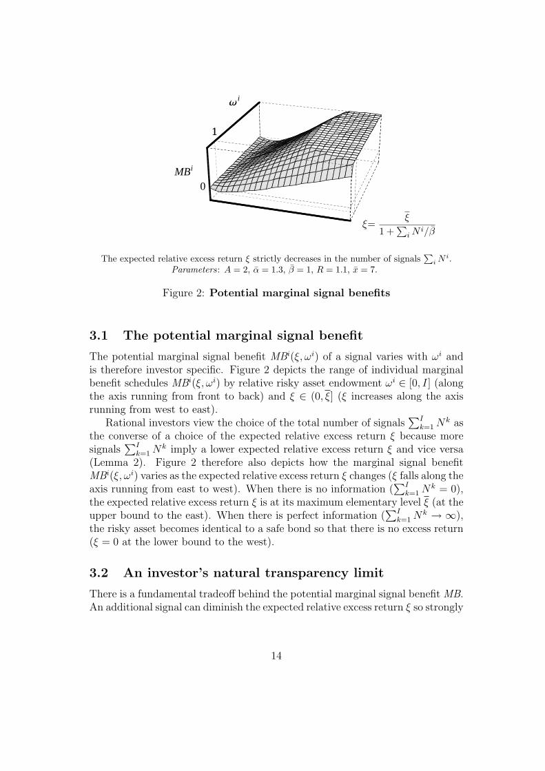
The expected relative excess return ξ strictly decreases in the number of signals∑

i N i.Parameters: A = 2, α = 1.3, β = 1, R = 1.1, x = 7.

ξ=ξ

1 +∑

i Ni/β

Figure 2: Potential marginal signal benefits

3.1 The potential marginal signal benefit

The potential marginal signal benefit MBi(ξ, ωi) of a signal varies with ωi andis therefore investor specific. Figure 2 depicts the range of individual marginalbenefit schedules MBi(ξ, ωi) by relative risky asset endowment ωi ∈ [0, I] (alongthe axis running from front to back) and ξ ∈ (0, ξ] (ξ increases along the axisrunning from west to east).

Rational investors view the choice of the total number of signals∑I

k=1 Nk asthe converse of a choice of the expected relative excess return ξ because moresignals

∑Ik=1 Nk imply a lower expected relative excess return ξ and vice versa

(Lemma 2). Figure 2 therefore also depicts how the marginal signal benefitMBi(ξ, ωi) varies as the expected relative excess return ξ changes (ξ falls along theaxis running from east to west). When there is no information (

∑Ik=1 Nk = 0),

the expected relative excess return ξ is at its maximum elementary level ξ (at theupper bound to the east). When there is perfect information (

∑Ik=1 Nk → ∞),

the risky asset becomes identical to a safe bond so that there is no excess return(ξ = 0 at the lower bound to the west).

3.2 An investor’s natural transparency limit

There is a fundamental tradeoff behind the potential marginal signal benefit MB.An additional signal can diminish the expected relative excess return ξ so strongly

14

ωi = 0 ωi = 18

ξ

MB,MC

0 ξ-ξ ω*ξ κ

*

ξ-

Signal Benefitante notitias

Signal Cost

ξ

MB,MC

0 ξ-ξ ω*ξ κ

*

ξ-

Signal Benefitante notitias

Signal Cost

ωi = 1 ωi = 8

ξ

MB,MC

0 ξ-ξ κ*

Signal Benefitante notitias

Signal Cost

ξ

MB,MC

0 ξ-ξ ω*ξ κ

*

Signal Benefitante notitias

Signal Cost

ξ-

The expected relative excess return ξ = ξ/(1 +∑

i N i/β) strictly decreases in∑

i N i.Parameters: A = 2, α = 1.3, β = 1, R = 1.1, x = 7, c = .1.

Figure 3: Potential marginal signal benefits by endowment

that this negative effect more than outweighs the benefits of information.10

Figure 3 depicts sections of the graph in Figure 2 for four relative risky assetendowments ωi and shows the individual marginal benefit schedules MBi(ξ, ωi).These sections could represent an economy with ten investors, for instance, whereeight investors hold ωi = 1/8 and one investor each holds ωi = 1 and ωi = 8.

Starting from zero information (at the eastern most excess return ξ = ξ),the individual marginal benefit schedule MBi(ξ, ωi) decreases monotonically inthe number of signals for every investor (as we move westwards). Ultimately,the potential marginal benefit MB of an additional signal reaches zero. Mostimportant, the potential marginal signal benefit MB turns strictly negative whenthe expected relative excess return ξ drops very far. Call the threshold where

10It can be shown for the case of a normal-normal pair of signal-return distributions thatthe diminishing effect of information on the expected excess return is so strong that the MBnever turns positive for ωi = 0 (an implication of Theorem 4, Muendler forthcoming). For aPoisson-gamma pair of distributions, however, the MB term in (11) can take a negative or apositive sign for ωi = 0.

15

the potential marginal signal benefit turns weakly negative investor i’s naturaltransparency limit ξi.

At the natural transparency limit ξi, investor i pays to inhibit further infor-mation disclosure. The potential benefit MB does not constitute a benefit buta cost once ξ falls below an investor’s natural transparency limit. The negativeMB for low ξ reflects that, given a relatively large number of available signals,the negative effect of an additional signal on the expected relative excess return ξoutweighs the benefit from a more informed expected portfolio choice ante noti-tias. A low ξ means that investors currently hold relatively many signals givenmarket size and the mean-variance ratio of the asset.

The transparency limit is investor specific because information revalues therisky asset, and the revaluation affects investors with heterogeneous endowmentsin different ways. The diminishing effect of an additional signal on the excessreturn ξ weighs heavily for investors with large initial risky asset positions be-cause ante notitias they are strongly affected by expected asset price volatility,anticipating that information will move price post notitias. The diminishing ef-fect of an additional signal on the excess return is also particularly strong forinvestors with no endowment of the risky asset (xi

0 = 0) since the increase in theopportunity cost RP is not mitigated by any positive wealth effect of asset priceon their endowments.

Facing the marginal utility cost of information MC, every investor comes upwith an individually optimal choice of ξ∗ωi given her relative stock endowment

ωi. When the elementary excess return ξ ≡ Ax/β (the maximal expected excessreturn absent information acquisition) is high, then a given choice of excessreturn ξ∗ωi requires a large amount of information acquisition, and vice versa.So, information demand is strong if many risky assets are in the market, or ifinvestors are highly risk averse, or if prior expectations of the mean-varianceratio of the asset return are relatively low so that uncertainty matters stronglycompared to expected returns.

Proposition 1 (Potential marginal signal benefit). The following is true for thepotential marginal signal benefit MB(ξ, ωi) under assumptions 1 to 5.

1. Investor i’s natural transparency limit ξi ∈ (0,∞) uniquely solves the zero

potential marginal signal benefit condition MB(ξi, ωi) = 0 given R∈(0,∞)

and ωi. The potential marginal signal benefit depends on ωi but not on ξ.

2. The potential marginal signal benefit MB(ξ, ωi) takes strictly positive valuesif and only if the prevailing expected relative excess return exceeds investori’s natural transparency limit ξ > ξi.

16

3. If investor i’s natural transparency limit is less than the elementary excessreturn ξi < ξ then, in the range ξ ∈ [ξi, ξ], the potential marginal signalbenefit MB(ξ, ωi) strictly monotonically increases in ξ and is unboundedfor arbitrarily large ξ.

4. If investor j has a risky asset endowment around the market average withωj ∈ [

√R/(

√1+R +

√R),

√1+R/(

√1+R − √

R)], then the potentialmarginal signal benefit MB(ξ, ωj) attains strictly positive values for anyξ ∈ (0, ξ] so that investor j’s natural transparency limit is infinite infor-mation.

Proof. See appendix F.

Proposition 1 establishes that there is an investor specific natural transparencylimit below which the investor pays to inhibit further disclosure. The naturaltransparency limit is unique for each investor i and is determined by the investor’srisky asset endowment ωi (statements 1 and 2). So, the incentive for informationacquisition varies with the risky asset endowment.

Proposition 1 also shows, however, that there is always a market size x, or adegree of risk aversion A, or a level of the prior mean-variance ratio of the riskyasset β behind ξ so that, for any investor i with endowment ωi, at least one costlysignal becomes worthwhile to acquire in equilibrium as x is raised (statement 3).

Finally, Proposition 1 identifies a range of risky asset endowments ωi ∈[√

R/(√

1+R+√

R),√

1+R/(√

1+R−√R)] where the potential marginal signalbenefit never turns negative (statement 4), not even as ξ approaches zero. Thisrange contains the market average endowment ωi = 1 as depicted in Figure 3.An investor with initial stock holdings in this range will hire unboundedly manyspy robots when their fee goes to zero.

These properties of the potential marginal signal benefit MB characterize theinformation market equilibrium in RICE. Signals are public goods and thereforeperfect strategic substitutes under fully revealing price because any fellow in-vestor’s signal is as useful (or detrimental) as an own signal. Consequently, theinformation market equilibrium does not pin down how many signals a singleinvestor holds. In RICE, one investor may acquire all

∑i N

i signals while no-body else buys any signal, or all investors may hold the same number of signals.Monotonicity of the individual potential marginal signal benefit schedules im-plies, however, that the equilibrium information level

∑Ik=1 Nk,∗ is unique.

Proposition 2 (Information market equilibrium). A RICE results in the fol-lowing informational outcomes for any R∈(0,∞) under assumptions 1 to 5.

1. If the cost of a signal is strictly positive, then the equilibrium informationlevel

∑Ik=1 Nk,∗ is unique.

17

2. If the cost of a signal is strictly positive, any permutation of the signalallocation that maintains the information level

∑Ik=1 Nk,∗ is an equilibrium.

3. If the cost of a signal is nil but R>0, and if there is at least one investor jwith a risky asset endowment ωj ∈ [

√R/(

√1+R+

√R),

√1+R/(

√1+R−√

R)], then the unique signal market equilibrium involves an infinite amountof freely received signals.

It remains to determine how investors arrive at∑I

k=1 Nk,∗ in the equilibriumfor spy robots.

3.3 Dominant investor valuation of signals

Information demand is intricately tied to investors’ risky asset endowments inRICE. There is, in fact, a single dominant investor with an above-average en-dowment of the risky asset. This dominant investor’s marginal signal valuationdominates everyone else’s valuation so that she single-handedly picks the infor-mation market outcome. In the sample economy of Figure 3, the average investorκ with ωκ =1 has the strongest incentive for information acquisition among theten investors and continues to acquire signals until the expected relative excessreturn ξ is diminished into a neighborhood around ξ∗κ. All other investors wouldstop acquiring signals earlier: at some expected relative excess return ξ∗ω > ξ∗κ.In Figure 3, the dominant investor κ’s endowment revaluation effect is so strongthat the individual marginal signal benefit MBκ never turns negative for anylevel of the expected relative excess return ξ. Proposition 3 shows that the dom-inant investor is to be found in an open set around investors with endowmentsof ωκ =1 and above.

The individual marginal signal benefit in equation (11) involves the expectedrelative excess return ξ and investor i’s relative risky asset endowment ωi innon-algebraic ways. Proposition 3 states properties of the information marketequilibrium for intervals of endowments.

Proposition 3 (Dominant Investor Valuation of Signals). A RICE has the fol-lowing allocation properties for any R∈(0,∞) under assumptions 1 to 5.

1. Given any ξ∗, the individual marginal signal benefit MB(ξ∗, ωκ) is maximalin equilibrium for a dominant investor κ. The dominant investor’s uniquerelative risky asset endowment falls into the interval ωκ

max MB ∈ (1, 1 +R(1+ξ∗)). This investor determines the total number of signals

∑Ik=1 Nk,∗

in equilibrium and diminishes expected relative excess return to ξ∗.

18

√1+R

√1+R−√R

√R

√1+R +

√R

0

Ωi

The expected relative excess return ξ strictly decreases in the number of signals∑

i N i.Parameters: A = 2, α = 1.3, β = 1, R = 1.1, x = 7.

ξ=ξ

1 +∑

i Ni/β

MB<0

ωi = 1

Figure 4: Contours of potential marginal signal benefits

2. The individual marginal signal benefit MB(ξ∗, ωi) at expected relative excessreturn ξ∗ is strictly positive for investors with endowments ωi in an openinterval Ω+ that includes [1, ωκ] ⊂ Ω+.

Proof. See appendix G.

Figure 4 shows contours of the potential marginal signal benefit MB(ξ, ωi)and serves to illustrate Proposition 3. Proposition 3 establishes that, for a givenequilibrium excess return ξ∗ (or any ξ), there is a unique ωκ

max MB that maxi-mizes the potential marginal signal benefit (statement 1). Equivalently, sinceMB(ξ, ωi) is monotonic in ξ when positive (Proposition 1), every marginal signalbenefit MB(ξ, ωi) contour must have one unique ωκ

max MB, for which ξ is minimal.Figure 4 depicts these ωκ

max MB as the western most points of the MB contours.Fix the marginal cost of a signal in utility terms, cAR/(1 + R). This cost

is the same for all investors by the first order condition (11). So, in equi-librium, the decisive investor must sit on the marginal signal benefit contourMB(ξ, ωi) = cAR/(1 + R). Pick any relative risky asset endowment ωj; theMB(ξ, ωi) contour returns the expected relative excess return ξ that investor

19

j finds optimal. Investor j will acquire signals until the expected relative ex-cess return in equilibrium is pushed down to her desired level. Move along theMB(ξ, ωi) to its western most point. This is the relative risky endowment levelof the unique dominant investor, ωκ

max MB ∈ (1, 1 + R(1 + ξ)), for whom theincentives to acquire information strictly exceed those of any other investor.

For investors with relative risky asset endowments below or above ωκmax MB,

the diminishing effect of signals on the expected excess return ξ weighs moreheavily. So, the investor with relative risky asset endowment ωκ

max MB single-handedly determines the information market outcome. This investor κ will con-tinue acquiring signals and diminish the expected relative excess return ξ untilthe total number of signals

∑Ik=1 Nk,∗ satisfies her first-order condition (11) for

signal demand. Proposition 3 also shows, however, that investors with relativerisky asset endowments in a range from below unity to above ωκ

max MB do not suf-fer a utility loss from the dominant investor’s signal choice (statement 2). Whatis the overall welfare impact of transparency?

4 Informational Efficiency

The rational Bayesian framework permits the application of a Pareto criterionto judge transparency in financial markets.

Definition 2 (Informational Pareto efficiency) An allocation of xi∗∗ risky assets,bi∗∗ safe bonds, and N i∗∗ signals to investors i = 1, ..., I is called informationallyPareto efficient in a given market environment (ξ, R) if there is no other allo-cation such that all investors are at least as well off and at least one investor isstrictly better off.

To investigate whether RICE is Pareto efficient, imagine a benevolent socialplanner who can instruct every consumer j to buy exactly N j∗∗ signals. Thissocial planner maximizes

∑Ij=1 Ei

ante [U j] with respect to N1, ..., N I. Thus,similar to Samuelson’s (1954) condition for public good provision, a benevolentsocial planner’s first-order conditions for information allocation are not (11) butinstead

− 1

Ejante [U

j]

∂∑I

k=1 Ekante

[Uk∗∗]

∂Nk= −A R

1+Rc (12)

+α

β

[(1 + ξ) exp

−ξ1+ξ

] 11+R

(1− 1

1+Rξ2

(1+ξ)2

)−1

1 +

([(1 + ξ) exp

−ξ1+ξ

] 11+R − 1

)ξξ

(1 +

I∑

k 6=j

Ekante

[Uk∗∗]

Ejante [U j∗∗]

)

20

SB,MB,MC

0 ξ-ξ *ξ **ξ-

Private Signal Benefitante notitias

Social Signal Benefitante notitias

Signal Cost

The expected relative excess return ξ strictly decreases in the number of signals∑

i N i.Parameters: A = 2, α = 1.3, β = 1, R = 1.1, x = 7, c = .1.

ξ=ξ

1 +∑

i Ni/β

Figure 5: Socially desirable information choice for homogeneous in-vestors

for any j ∈ 1, ..., I, written in terms of that investor j’s utility. Thus, com-pared to the privately perceived benefits, the potential social benefits SB thata social planner considers scale up the private benefits MB by a factor of 1 +(1/Ej

ante [U j∗∗]) ·∑Ik 6=j Ek

ante

[Uk∗∗] > 1.

4.1 Welfare effects for homogeneous investors

To simplify the welfare analysis, consider the case of I−1 homogeneous investorswith ωi = 0 and one single owner j of the risky asset with ωj = I. The upper leftand lower right graphs in figure 3 exemplify this case for a sample economy withI = 8 investors, seven of whom hold ωi = 0 while one owns ωj = I = 8. Neitherthe sole owner nor investors with safe endowments may value information much.In fact, the marginal signal benefit approaches negative infinity for the sole ownerof a risky project as her relative risky asset endowment ωj (the project size Ix)increases for a given average endowment x (claim 4 in appendix G).

Not even for homogeneous investors with no initial risky asset holdings needinformation be desirable. Proposition 1 implies that signals can turn from apublic good into a public bad as market conditions change. These market con-ditions are captured by ξ. If ξ drops below the homogeneous investors’ jointtransparency limit, information becomes a public bad, and a benevolent socialplanner wants to implement an even smaller amount of information than theprivate market. For no information is acquired in private markets in that case

21

anyway, the market equilibrium is informationally efficient when information isa public bad.

On the other hand, if information is a public good under given market con-ditions, a social planner wants (weakly) more information to be allocated thanmarkets provide. Individual investors do not take into account that their signalacquisition also benefits other investors through fully revealing price. In thiscase, markets allocate (weakly) less information than desirable. Signals are notdivisible, however, and we cannot infer from condition (12) that a social plannerwants to implement strictly more information. In Figure 5, a social planner wantsto allocate information so that the relative excess return is brought down fromaround ξ∗ to around ξ∗∗. If a single additional signal makes the implementablelevel of ξ drop far below ξ∗∗, however, investors could be better off if relativeexcess return ξ remains at the market equilibrium level around ξ∗.

Even if signals are free with c = 0, only the market outcome with finiteinformation is efficient but not the one with infinite information. As long as thebond is valuable (R > 0), neither markets nor the social planner want to removeuncertainty. In incomplete markets, investors with no initial risky asset holdingsprefer to have a second asset around that is not a perfect substitute to the bond.Risk-averse investors want to hold risky assets that yield a positive excess returnξ over opportunity cost. Only if the bond becomes useless and R → 0, doesunbounded information Pareto become efficient.

4.2 Welfare effects for heterogeneous investors

The welfare analysis changes considerably when endowments with the risky as-set differ across investors. Now, one dominant investor κ with close-to-market-average holdings of the risky asset determines the equilibrium number of signalin RICE (Proposition 3). Investors with endowments in an open interval around[1, ωκ] strictly benefit from investor κ’s additional information choice since theirmarginal utility benefit of signals is strictly positive and they do not have to payfor the public good.

For investors outside the open set of endowments of ωκ =1 and above, how-ever, the individual marginal signal benefit MBi(ξ, ωi) can turn strictly negativeeven in the presence of the endowment revaluation effect. Reduce the signalcost in Figure 3, for instance. Then the individual marginal benefit schedulesMBi(ξ, ωi) can dip into the strictly negative range before investor κ reaches hernatural transparency limit. Similarly, consider the western-most (strictly posi-tive) potential marginal benefit contour in Figure 4. At the equilibrium outcomeξ∗ for the dominant investor on this contour, the potential marginal signal benefithas turned strictly negative for investors at the extremes of the ωi distribution.

22

Formally, at any ξ, the marginal signal benefit approaches negative infinity as ωi

increases for a given average endowment x (claim 4 in appendix G). So, when thedistribution of risky asset endowments is unequal and many investors hold riskyasset endowments far from average, the dominant investor’s information choiceinflicts a strict negative externality on numerous investors. If, on the other hand,investors’ risky asset endowments are distributed closely around the market av-erage, the endowment revaluation effect makes signals similarly valuable to allinvestors. Proposition 4 summarizes these insights.

Proposition 4 (Informational Efficiency). A RICE has the following informa-tional efficiency properties for any R∈(0,∞) under assumptions 1 to 5.

1. If every investor i’s endowment ωi falls into the interval ωi ∈ [1, ωκ], whereωκ is the dominant investor κ’s endowment (Proposition 3), then RICE isnot informationally Pareto efficient. Up to discrete tolerance, an increasein the number of signals raises every investor’s ante notitias utility.

2. If there is one investor j with an endowment outside the range where infi-nite information is beneficial, ωj /∈ [

√R/(

√1+R+

√R),

√1+R/(

√1+R−√

R)], then there is an information cost c low enough so that RICE is in-formationally Pareto efficient. An increase in the number of signals strictlyreduces investor j’s ante notitias utility while, up to discrete tolerance, theincrease in the number of signals strictly raises the dominant investor’sante notitias utility.

Information acquisition creates a two-group society of investors. The endow-ment revaluation effect of more signals strictly outweighs the diminishing effecton the expected excess return ξ for a first group of investors in an open set Ω+

of relative risky asset endowments around [1, ωκ] ⊂ Ω+ (Proposition 3). In fact,given the choice of free signals, investors k with endowments inside the rangeωk ∈ [

√R/(

√1+R +

√R),

√1+R/(

√1+R − √

R)] (Proposition 1), would re-move all uncertainty from the market—just to enjoy the endowment revaluation.

For the second group of investors, endowments are either too small so that thediminishing effect on the expected excess return starts to outweigh the endow-ment revaluation effect at some small enough ξ, or endowments are too large sothat the expected variance of price outweighs the endowment revaluation effectat some small enough ξ. Outside the endowment range where infinite costlessinformation is beneficial (outside [

√R/(

√1+R+

√R),

√1+R/(

√1+R−√R)]),

the marginal ante notitias utility of an additional signal is strictly negative forlow ξ. The second group of investors suffers a strict negative externality in antenotitias utility terms from the rush to information of the first group of investors.

23

The Pareto criterion applied to a social planner’s transparency choice loses itsbite: investors in the second group are worse off with every additional signal.

Overall, transparency leads to an unambiguous Pareto improvement only inmarkets with sufficiently similar investors—after the risky asset has been issuedand all investors hold it in their initial portfolios to some degree. If an asset hasnot been issued yet so that only one agent holds the asset in his or her initialendowment, public disclosure can violate everyone’s transparency limit.

4.3 Asset price precision

Most commonly, the informational efficiency of financial markets is judged withcriteria that do not relate to welfare but to the degree of information transmis-sion through asset price. Fama (1970) discerns three degrees of market efficiencyin this welfare-independent sense: Strong, semi-strong, and weak. Prices arefully revealing in RICE under the assumptions of this paper (Lemma 3 in ap-pendix C). So, Ei [RP − Ei [RP ]] = 0 and RICE satisfies strong-form efficiency.An alternative statistically well defined measure of the informativeness of a signalis its precision, the inverse of the ante notitias variance. Informational efficiencyin this non-welfare sense relates to price as a source of information.

The precision of price, a Poisson variable by (4) and fact 3 (appendix B), is

1

Eiante [Vi (P |θ)] =

β2

α

((1 + ξ) +

∑Ii=1 N i∗/β

)2

∑Ii=1 N i∗/β

.

So, the precision of price can fall with the number of signals purchased. For

∂

∂N i

(1

Eiante [Vi (P |θ)]

)=

β

α

(∑I

i=1 N i∗/β)2 − (1 + ξ)2

(∑I

i=1 N i∗/β)2,

each additional signal reduces the precision of the market clearing price if theamount of pre-existing information

∑Ik=1 Nk,∗ is small.

Proposition 5 (Precision loss of the price system). In asset market REE underassumptions 1 through 4, the ante notitias precision of the price system decreaseswith every additional signal if and only if

∑Ik=1 Nk,∗/β < 1 + ξ.

Precision of price can fall with the number of signals purchased.11 Each in-vestor anticipates that she and all others will respond to signals in their portfolio

11Bushee and Noe (2000) provide empirical evidence that more information may worsen pricevolatility.

24

choice. From an ante notitias perspective, asset demand (4) can become morevolatile with the anticipated arrival of information. The expected variance ofasset demand is

Eiante

[Vi

(xi∗|θ) |RP

]=

α

βA2(RP )2

(I∑

k=1

Nk

)

by fact 3. Financial markets need to clear and every investor ends up hold-ing x risky assets in equilibrium by Proposition 3, irrespective of information.Hence, market price has to fully absorb any demand moves that stem from in-formation revelation. As a consequence, the variance of price can increase withmore information acquisition. When there is relatively little pre-existing infor-mation

∑Ik=1 Nk,∗, an additional signal will affect individual demands strongly

and thus add to the price’s variance. If, on the other hand, a lot of information isavailable already, an additional signal that gets fully revealed through price willmove investors’ demands little. If investors receive many signals, an additionalpiece of information is likely to confirm previous observations and tends to sta-bilize demand. So, equilibrium price is expected to become less volatile with anadditional signal if the pre-existing information level

∑Ik=1 Nk,∗ is high.

Rational investors completely internalize this change in price volatility whenthey maximize ante notitias utility. In that sense, the precision of price is irrel-evant for the Pareto efficiency of RICE.

5 Conclusion

By adding a stage of signal acquisition to a canonical model of portfolio choice,this paper has shown that investors with heterogeneous initial holdings of therisky asset find financial transparency, even if free, only desirable to a degree. Inreducing uncertainty, transparency raises expected asset price and thus benefitsholders of the risky asset. At their natural transparency limits, however, investorspay to inhibit further disclosure in order to prevent the information-inducedincrease in expected asset price and to avert an erosion of the asset’s expectedexcess return. The natural transparency limit varies with an investor’s initialportfolio position. The natural transparency limit shifts to perfect informationfor investors around the market average risky asset endowment because theseinvestors benefit most from rising expected asset price. There is, in fact, adominant investor with a risky asset endowment modestly above market averagewho keeps acquiring signals after all other investors’ demand for transparency isexhausted. The dominant investor’s transparency choice strictly improves welfarefor investors with similar (modestly smaller or larger) risky asset endowments.

25

Investors with strongly different risky asset endowments, however, suffer a strictwelfare loss if the dominant investor keeps acquiring signals beyond their naturaltransparency limits.

Financial transparency not only changes its utility benefit with market con-ditions. Transparency raises expected asset price and thus also affects investors’portfolio positions ante notitias. So, the value of public signals is intricatelylinked to the distribution of risky asset endowments across heterogeneous in-vestors. This poses an intriguing problem for the analysis of informational ef-ficiency in the presence of heterogeneous investors. A common distinction ineconomics between pure allocative efficiency in the Pareto sense and distributivejudgements is hard to uphold for financial information in a rational Bayesianframework.

Extensions of the framework in this paper remain for future work: an analysisof information values in complete markets, an investigation of partially revealingequilibrium (such as for investors with different degrees of risk aversion), and theconsideration of investors who engage in strategic demand decisions to partlyconceal their information. The driving force behind the effects of transparency,however, is the diminishing effect of information on an asset’s excess return. In-formation diminishes the asset’s excess return because a sufficient statistic ofprivate signals is publicly inferrable from price. Neither complete markets norpartially revealing equilibrium nor strategic investors can make asset price en-tirely uninformative, or else price would lose its allocation function. So informa-tion continues to diminish excess returns in those settings albeit in a mitigatedmanner (Admati 1985, Easley and O’Hara 2004). It thus appears plausible thatmain results of this paper will carry over to generalizations and extensions.

26

Appendix

A Optimality conditions and portfolio value

Define t ≡ −Axi ∈ (−∞, 0) for the moment generating function (MGF) Mθ|Fi(t).Maximizing (3) over xi and bi for CARA (assumption 2 and 3) yields the first-order conditions

P

ρi= H i M ′

θ|Fi(t) and1

ρiR= H i Mθ|Fi(t), (A.1)

where H i ≡ exp−A[(1+R)bi + Pxi −W i0 − cN i]. Note that H i, W i

0, Ci1 and

C i0 are functions of F i since RP depends on F i.

With the definition of H i, the optimal portfolio value can be written

bi + Pxi = 11+R

(W i

0 − cN i + RP xi − 1A

ln H i)

(A.2)

= 11+R

[bi0 + RP (xi

0/R + xi) + 1A

ln ρiRMθ|Fi(−Axi)− cN i],

where the second line follows from the bond first-order condition in (A.1).The matrix of cross-derivatives for the two assets bi and xi reflects the second-

order conditions:

B = −A2ρi exp−ARbi∣∣∣∣R(1+R)Mθ|Fi(t) ·(1+R)M ′

θ|F i(t) PM ′θ|Fi(t) + M ′′

θ|Fi(t)

∣∣∣∣ (A.3)

by (A.1). If B is negative definite, a unique global utility maximum results.Equivalently, require −B to be positive definite and all upper-left sub-matricesmust have positive determinants. Since the upper-left entry in B is strictlypositive, negative definiteness of B is equivalent to

det(−B) = A4(ρi)2 exp−2ARbiR(1+R)[M ′′

θ|Fi(t)Mθ|Fi(t)−M ′θ|Fi(t)2

]> 0,

which in turn is equivalent to

M ′′θ|Fi(t)

Mθ|Fi(t)−

(M ′

θ|Fi(t)

Mθ|Fi(t)

)2

> 0 (A.4)

since Mθ|Fi(t) > 0. This condition implies that M ′θ|Fi(t)/Mθ|Fi(t) strictly mono-

tonically increases in t, or strictly monotonically decreases in xi for t ≡ −Axi.The condition is satisfied for a gamma distribution.

27

B Poisson and gamma distributions

Fact 1 in the text states how Poisson signals update beliefs about gamma dis-tributed returns. This appendix lists further useful properties of Poisson andgamma distributions

B.1 Poisson signals

Poisson distributed signals Sin|θ i.i.d.∼ P(θ) have a density

f(si

n |θ)

=

exp−θ θsi

n/sin! for si

n > 00 for si

n ≤ 0

Fact 2 (Poisson MGF). The MGF of a Poisson signal is

MS|θ(t) = expθ(expt − 1).Proof. Casella and Berger (1990).

Fact 3 (Sum of Poisson signals). The sum of N independently Poisson dis-tributed signals with a common mean and variance θ, S1 + ...+SN , has a Poissondistribution with parameter Nθ.

Proof. The distribution of the sum of N independent Poisson variables is theproduct ΠN

n=1f (sin |θ ) = exp−Nθ θ

∑Nn=1 si

n/∑N

n=1 sin!, a Poisson distribution

with parameter Nθ.

B.2 Gamma payoffs

Given an individual investor i’s information set αi, βi, the risky asset payoff isdistributed θ ∼ G(αi, βi) so that its density is

π(θ∣∣αi, βi

)=

(βi)αi

θαi−1 exp−βiθ/Γ(αi) for θ > 00 otherwise

where the gamma function is given by Γ(αi) ≡ ∫∞0

zαi−1e−z dz. The two param-eters αi and βi must be positive.

Fact 4 (Gamma MGF). The MGF of a gamma distributed return is

Mθ|αi,βi(t) =

(βi

βi − t

)αi

.

Proof. Casella and Berger (1990).

28

C Conditions for fully revealing price

Lemma 3 Suppose signals are Poisson, the asset return is gamma distributed(assumption 1), and expected utility is CARA (assumption 2). Then equilibrium

price P fully reveals all investors’ information∑I

i=1

∑N i

n=1 sin in RICE if and only

if

1. investors know average prior beliefs and share a common degree of riskaversion (a weaker version of assumption 3),

2. investors know market size (assumption 4),

3. investors know the total number of all other investors’ signals∑I

k=1 Nk atthe time of portfolio choice, and

4. investors are not borrowing constrained.

Proof. Lemma 1 establishes sufficiency. Necessity of assumptions 3 and 4 followsby inspection of the general solution for market price given individual beliefs

αi = αi +∑N i

n=1 sin and βi = βi + N i, based on heterogeneous priors αi and βi,

and arbitrary degrees of risk aversion Ai:

RP =1I

∑Ii=1

αi

Ai

x +∑I

i=1βi

Ai

=

(1I

∑Ii=1

αi

Ai

)+ 1

I

∑Ii=1

1Ai

∑N i

n=1 sin

x +(

1I

∑Ii=1

βi

Ai

)+ 1

I

∑Ii=1

1Ai N i

.

If investors have a common degree of risk aversion Ai = A, only knowledge ofthe average prior beliefs 1

I

∑Ii=1 αi and 1

I

∑Ii=1 βi is necessary to make price fully

revealing.Conditional independence of signals is necessary since investor i would not

know the correlation between RP and her signals if perfect copies or correlatedsignals had been sent to other investors. If

∑Ik=1 Nk were unknown to investor

i, she would not be able to extract the sufficient statistic∑I

k=1

∑Nk

n=1 skn from

price.For necessity of unconstrained borrowing, consider the case in which some

investors cannot go short in the risky asset due to a borrowing constraint. Thenanother investor will not know whether the equilibrium price is low because manyrelatively poor investors received bad signals and hit their borrowing constraintor whether only a few relatively wealthy investors received extremely bad signals.As a consequence, price uncertainty remains.

29

D Bond return response to stock information

Taking logs of both sides of the bond first-order condition in (A.1) yields

A(1+R)bi − Abi0 + AP (xi − xi

0) = ln[ρiRMθ|Fi(−A xi)] + AcN i,

a permissible operation since ρi, R,Mθ|Fi(·) > 0 by their definitions. Summingup both sides over investors i and dividing by their total number yields

ARb− ln ρiR− ln Mθ|Fi(t)− Ac∑I

k=1 Nk/I = 0 (D.1)

where b ≡ ∑Ii=1 bi

0/I is the average initial bond endowment per investor and t ≡−Ax. Equation (D.1) implicitly determines the gross bond return R. Post noti-

tias, Mθ|Fi(t) and R respond to the signal realization. Define s ≡ ∑Ik=1

∑Nk

n=1 skn.

Applying the implicit function theorem to (D.1) for the MGF of the gammadistribution Mθ|α,β(t) = [β/(β − t)]α yields

dR

ds= − ln(1 + ξ)

Ab− 1/R

for α = α + s, β = β +∑I

k=1 Nk by (6) and ξ = Ax/β given∑I

k=1 Nk. Thebond return falls in response to a favorable signal realization s iff b > 1/(AR).So, in principle, R too is a function of the signal realization s. For large bondendowments b, however,

limb→∞

dR/ds = 0.

Similarly, dR/ds = 0 for ξ = x = 0.

E Ante notitias expected indirect utility

The following property of the Poisson-gamma signal-return distributions provesuseful for the derivation of ante notitias expected indirect utility.

Fact 5 (Expected signal effect on utility). For two arbitrary constants B and ξ,N Poisson distributed signals S1, ..., SN and a conjugate prior gamma distributionof their common mean θ, the following is true:

Eante

(1 + ξ)

−B·N∑

n=1sn · exp

− ξ(ωi−1)

1+ξB ·

N∑n=1

sn

= (1 + ξ)αB exp

α ξ(ωi−1)1+ξ

B(

1 +[(1 + ξ)B exp

ξ(ωi−1)

1+ξB

− 1

]ββ

)−α

,

where α and β are the parameters of the prior gamma distribution of θ, andβ = β + N is the according parameter of the post notitias distribution.

30

Proof. By iterated expectations Eante [·] = Eθ [E [· |θ ]]. The ‘inner’ expectationE [· |θ ] is equal to

E [· |θ ] =∑∞

(∑N

n=1sn)= 0(1 + ξ)

−BN∑

n=1sn

exp

− ξ(ωi−1)

1+ξB

N∑n=1

sn

f

(∑Nn=1 sn

)

= exp−Nθ

(1− (1 + ξ)−B exp

− ξ(ωi−1)

1+ξB

),

because the sum∑N

n=1 sn is Poisson distributed with mean Nθ (fact 3). Thus,by the MGF of a gamma distribution (fact 4),

Eante [·] = Eθ

[exp

−θ

(1− (1 + ξ)−B exp

− ξ(ωi−1)

1+ξB

)(β − β)

]

= (β)α(β +

(1− (1 + ξ)−B exp

− ξ(ωi−1)

1+ξB

)(β − β)

)−α

.

since N = β − β (fact 1). Simplifying the last term and factoring out (1 +

ξ)B exp ξ(ωi−1)1+ξ

B proves fact 5.

For a gamma distributed asset return, post notitias expected indirect utilitybecomes

Ei [U i∗] = −δi exp−A R

1+R(W i

0 − cN i)

exp

ξ(ωi−1)1+ξ

− αi

1+R(1 + ξ)−

αi

1+R (E.1)

where ωi ≡ xi0/x ∈ [0, I] is the relative endowment of investors with the risky

asset, and ξ ≡ Ax/β. With fact 5 at hand, one can set B ≡ 1/(1 + R) (byassumption 5) and obtains ante notitias expected utility (10) for ωi = 0 and (10)for arbitrary ωi ∈ [0, I].

F Monotone marginal signal benefit schedule

(proof of Proposition 1)

Define the relative endowment of investors with the risky asset as ωi ≡ xi0/x ∈

[0, I]. The expected relative excess return ξ is bounded by ξ ∈ (0, ξ]. Un-der assumptions 1 through 5, the potential marginal signal benefit MB(ξ, ωi)is MB(ξ, ωi) = g(ξ, ωi)/h(ξ, ωi) by (11) with

m(ξ, ωi) ≡[(1 + ξ) exp

ξ(ωi−1)

1 + ξ

] 11+R

, (F.1)

h(ξ, ωi) ≡ 1 +[m(ξ, ωi)− 1

] ξ

ξ, (F.2)

g(ξ, ωi) ≡ −ξ2

ξ

∂h(ξ, ωi)

∂ξ= m(ξ, ωi)

(1− 1

1+R

ξ(ξ+ωi)

(1 + ξ)2

)−1. (F.3)

31

The proof of Proposition 1 proceeds in four steps.First, claim 1 sates useful properties of m(ξ, ωi) for the discussion of g(ξ, ωi)

and h(ξ, ωi). Second, claim 2 establishes that the numerator g(ξ, ωi) strictlyincreases in ξ iff ξ > |ωi−1|

√1 + 1/R − ωi and that it is not bounded above.

So, the numerator boosts the marginal benefit MB(ξ, ωi) higher and higher asξ rises. Third, claim 3 establishes that the denominator h(ξ, ωi) is boundedbelow and above in the positive range, and that it strictly decreases in ξ iff thenumerator is strictly positive. So, the denominator cannot explode and booststhe marginal benefit MB(ξ, ωi) higher where the potential benefit MB(ξ, ωi) ispositive. The latter two claims imply that MB(ξ, ωi) strictly increases in ξ iffξ > |ωi−1|

√1 + 1/R− ωi and that MB(ξ, ωi) is unbounded for arbitrarily large

ξ. So, fourth and last, MB(ξ, ωi) ultimately attains strictly positive values andcontinues to strictly increase in that positive range.

Claim 1 m(ξ, ωi) strictly increases in ωi; m(0, ωi) = 1; and m(ξ, ωi) > 1 forany ξ > 0, ωi ≥ 0 and R∈(0,∞).

Proof. By (F.1), ∂m(ξ, ωi)/∂ξ = m(ξ, ωi)ξ/(1 + ξ) > 0, which establishes thefirst part of the claim.

Taking natural logs of both sides of (F.1) is permissible since m(ξ, ωi) > 0and shows that m(ξ, ωi) ≥ 1 iff ln(1 + ξ) ≥ −ξ(ωi−1)/(1 + ξ). Since m(ξ, ωi)strictly increases in ωi, consider ωi = 0. So, m(ξ, 0) ≥ 1 iff ln(1+ ξ) ≥ ξ/(1 + ξ).Note that equality holds at ξ = 0 but ln(1 + ξ) increases strictly faster in ξ thanξ/(1 + ξ) increases in ξ for any ξ > 0. So, m(ξ, 0) > 1. Since m(ξ, ωi) strictlyincreases in ωi, m(ξ, ωi) > 1.

Claim 2 g(ξ, ωi) strictly increases in ξ iff ξ > |ωi−1|√

1 + 1/R−ωi. In addition,limξ→0 g(ξ, ωi) = 0 and limξ→∞ g(ξ, ωi) = +∞.

Proof. The first derivative of g(ξ, ωi) with respect to ξ is

∂g(ξ, ωi)

∂ξ=

ξ

(1+R)2(1+ξ)4m(ξ, ωi)

[R(ξ + ωi)2 − (1+R)(ωi − 1)2

].

So, ∂g(ξ, ωi)/∂ξ = 0 at ξ = 0 and at ξ = |ωi−1|√

1 + 1/R − ωi (the negativeroot is ruled out by ξ ≥ 0). Evaluating ∂g(ξ, ωi)/∂ξ = 0 around the zero pointsshows that g(ξ, ωi) strictly decreases in ξ if ξ ∈ (0, |ωi−1|

√1 + 1/R − ωi) and

strictly increases if ξ ∈ (|ωi−1|√

1 + 1/R− ωi,∞).limξ→0 g(ξ, ωi) = m(0, ωi) − 1 = 0 by claim 1. limξ→∞ g(ξ, ωi) = −1 +

limξ→∞ expξ/(1 + R) = +∞ since R∈(0,∞).

32

Claim 2 implies that, if |ωi−1|√

1 + 1/R − ωi > 0, then there must be a

strictly positive ξi > |ωi−1|√

1 + 1/R − ωi that solves g(ξi, ωi) = 0 because

g(ξ, ωi) strictly decreases as long as ξ < |ωi−1|√

1 + 1/R− ωi but subsequently

strictly increases in ξ. If |ωi−1|√

1 + 1/R− ωi ≤ 0, however, then g(ξi, ωi) = 0

only at ξi = 0.

Claim 3 h(ξ, ωi) strictly decreases in ξ iff g(ξ, ωi) > 0. h(ξ, ωi) is bounded inh(ξ, ωi) ∈ (1, h(ξi, ωi)] for any ξ ∈ (0, ξ] and R∈ (0,∞), where ξ is given by (9)

and ξi solves g(ξi, ωi) = 0. Moreover, h(ξi, ωi) > 1.

Proof. By (F.3), ∂h(ξ, ωi)/∂ξ < 0 iff g(ξ, ωi) > 0. So, h(ξ, ωi) attains its globalmaximum at ξi, which solves g(ξi, ωi) = 0, and h(ξ, ωi) attains its minimumeither if ξ → 0 or if ξ → ∞. By L’Hopital’s rule, limξ→0 m(ξ, ωi)/ξ − 1/ξ = 0so limξ→0 h(ξ, ωi) = 1. Similarly, for any R∈ (0,∞), limξ→∞ h(ξ, ωi) = 1 (but,as R → 0, limξ→∞ h(ξ, ωi) = 1 + ξ expωi − 1). This establishes that h(ξ, ωi) ∈(1, h(ξi, ωi)] for any ξ ∈ (0, ξ].

Claims 2 and 3 imply that, if |ωi−1|√

1 + 1/R − ωi > 0, then MB(ξ, ωi)

strictly increases in ξ iff ξ > |ωi−1|√

1 + 1/R− ωi and MB(ξ, ωi) is unboundedfor arbitrarily large ξ. So, MB(ξ, ωi) attains strictly positive values if and only ifξ > ξi, where ξi > |ωi−1|

√1 + 1/R−ωi > 0 solves g(ξi, ωi) = 0, and ξi∈(0,∞)

is independent of ξ and unique given R∈(0,∞).If |ωi−1|

√1 + 1/R−ωi ≤ 0, however, then MB(ξ, ωi) attains strictly positive

and increasing values for any ξ ∈ (0, ξ]. |ωi−1|√

1 + 1/R− ωi ≤ 0 is satisfied if

ωi ∈ [√

R/(√

1+R +√

R),√

1+R/(√

1+R−√R)].

G Dominant investor valuation of signals

(proof of Proposition 3)

Define the relative endowment of investors with the risky asset as ωi ≡ xi0/x ∈

[0, I]. The expected relative excess return ξ is bounded by ξ ∈ (0, ξ]. Un-der assumptions 1 through 5, the potential marginal signal benefit MB(ξ, ωi)is MB(ξ, ωi) = g(ξ, ωi)/h(ξ, ωi) by (11) with h(ξ, ωi) and g(ξ, ωi) given by (F.3)and (F.2).

The proof of the remainder of Proposition 3 draws on properties of g(ξ, ωi)and h(ξ, ωi), which claims 4 and 5 establish. Claim 6 evaluates the potentialmarginal signal benefit MB(ξ, ωi) at ωi = 1.

Claim 4 g(ξ, ωi) strictly decreases in ωi iff ωi > 1 + R(1 + ξ). In addition,limωi→∞ g(ξ, ωi) = −∞.

33

Proof. The first derivative of g(ξ, ωi) with respect to ωi is

∂g(ξ, ωi)

∂ωi=

1

1+R

ξ2

(1+ξ)2m(ξ, ωi)

[R(1 + ξ)− (ωi − 1)

],

where m(ξ, ωi) is given by (F.1). So, ∂g(ξ, ωi)/∂ωi = 0 at ωi = 1 + R(1 + ξ).Evaluating ∂g(ξ, ωi)/∂ξ = 0 around this unique zero point shows that g(ξ, ωi)strictly increases in ωi if ωi ∈ [0, 1 + R(1 + ξ)) and strictly increases if ωi ∈(1 + R(1 + ξ), I]. So, limωi→∞ g(ξ, ωi) = −∞ for R∈(0,∞) and ξ∈(0, ξ].

Claim 5 h(ξ, ωi) strictly increases in ωi and is strictly convex in ωi at any ξ > 0.

Proof. The first and second derivatives of h(ξ, ωi) with respect to ωi are

∂h(ξ, ωi)

∂ωi=

1

1+R

ξ

1+ξm(ξ, ωi) > 0

and∂2h(ξ, ωi)

∂(ωi)2=

1

1+R

ξ

1+ξ

∂h(ξ, ωi)

∂ωi> 0.

Claim 6 The potential marginal signal benefit MB(ξ, 1) is strictly positive atωi = 1 for ξ >0,R>0. At ωi = 1, the potential marginal signal benefit MB(ξ, 1)strictly increases in ωi.

Proof. At ωi = 1, MB(ξ, 1) > 0 iff

11+R

ln(1 + ξ) > − ln(1− 1

1+Rξ

1+ξ

).

Note that equality holds at ξ = 0 but the left-hand side increases strictly fasterin ξ (it increases by 1/(1+R)(1+ξ)) than the right-hand side increases (whichincreases in ξ by 1/(1+ξ)2[1+R− ξ/(1+ξ)]) for any ξR > 0. So, MB(ξ, 1) > 0.

The first derivative of MB(ξ, ωi) with respect to ωi is

∂MB(ξ, ωi)

∂ωi=

(∂g(ξ, ωi)/∂ωi

g(ξ, ωi)− ∂h(ξ, ωi)/∂ωi

h(ξ, ωi)

)MB(ξ, ωi).

So, ∂MB(ξ, ωi)/∂ωi > 0 at ωi = 1 iff(

∂g(ξ, ωi)/∂ωi

g(ξ, ωi)

/∂h(ξ, ωi)/∂ωi

h(ξ, ωi)

)∣∣∣∣∣ωi=1

> 1 (G.1)

34

since h(ξ, ωi) > 1 by claim 3 and ∂h(ξ, ωi)/∂ωi > 1 by claim 5 for ξ>0. A roundof simplifications shows that inequality (G.1) is equivalent to

ξ(ξ + ξR) > ξ(1+R)[(1+ξ)

11+R − 1

].

Note that this condition holds with equality at ξ = 0 but the left-hand sideincreases strictly faster in ξ (it increases by ξ(1+2Rξ/ξ) > ξ) than the right-hand

side increases (which increases in ξ by ξ(1+ξ)−1

1+R < ξ). So, ∂MB(ξ, 1)/∂ωi > 0.

These claims help establish Proposition 3. g(ξ, ωi) attains its unique maxi-mum in ωi at ωi = 1 + R(1 + ξ) by claim 4 while h(ξ, ωi) strictly increases inωi but is convex. So, given any ξ, MB(ξ, ωi) must attain its global maximumat some ωκ < 1 + R(1 + ξ). At ωi = 1, MB(ξ, 1) strictly increases. This provesthe first statement of Proposition 3 that, given any ξ, MB(ξ, ω) must attain itsunique global maximum for some ωκ ∈ (1, 1 + R(1 + ξ)). The second statementthat MB(ξ, ω) > 0 for ω in an open interval Ω+ that includes [1, ωκ] ⊂ Ω+ fol-lows because MB(ξ, ωi) is strictly positive and strictly increases at ω = 1 for anyξ > 0. So, MB(ξ, ω) > 0 in an open interval around ω = 1. MB(ξ, ω) is maximalat ωκ so that the open interval Ω+ must in fact extend to [1, ωκ] ⊂ Ω+.

35

References

Admati, Anat R., “A Noisy Rational Expectations Equilibrium for Multi-asset Se-curities Markets,” Econometrica, May 1985, 53 (3), 629–57.

Angeletos, George Marios and Alessandro Pavan, “Transparency of Informationand Coordination in Economies with Investment Complementarities,” AmericanEconomic Review, May 2004, 94 (2), 91–98.

Bolton, Patrick and Christopher Harris, “Strategic Experimentation,” Econo-metrica, March 1999, 67 (2), 349–74.

Bushee, Brian J. and Christopher F. Noe, “Corporate Disclosure Practices, Insti-tutional Investors, and Stock Return Volatility,” Journal of Accounting Research,Supplement 2000, 38, 171–202.

Casella, George and Roger L. Berger, Statistical inference, 6th ed., New York:Duxbury, June 1990.

Cripps, Martin William, Godfrey Keller, and Sven Rady, “Strategic Experi-mentation with Exponential Bandits,” Econometrica, January 2005, 73 (1), 39–68.

Davis, Ronald E., “Certainty-Equivalent Models for Portfolio Optimization UsingExponential Utility and Gamma-Distributed Returns,” in Kenneth D. Lawrence,John B. Jr. Guerard, and Gary R. Reeves, eds., Advances in mathematical pro-gramming and financial planning, Vol. 3, Greenwich, CT and London: JAI Press,1993, pp. 69–108.

Diamond, Douglas W., “Optimal Release of Information by Firms,” Journal ofFinance, September 1985, 40 (4), 1071–94.

Easley, David and Maureen O’Hara, “Information and the Cost of Capital,”Journal of Finance, August 2004, 59 (4), 1553–83.

, Soeren Hvidkjaer, and Maureen O’Hara, “Is Information Risk a Determi-nant of Asset Returns?,” Journal of Finance, October 2002, 57 (5), 2185–2221.

Fama, Eugene F., “Efficient Capital Markets: A Review of Theory and EmpiricalWork,” Journal of Finance, May 1970, 25 (2), 383–417.

Grossman, Sanford J. and Joseph E. Stiglitz, “On the Impossibility of Infor-mationally Efficient Markets,” American Economic Review, June 1980, 70 (3),393–408.

Heston, Steven L., “Invisible Parameters in Option Prices,” Journal of Finance,July 1993, 48 (3), 933–47.

36

Kim, Oliver and Robert E. Verrecchia, “Market Reaction to Anticipated An-nouncements,” Journal of Financial Economics, December 1991, 30 (2), 273–309.

Krebs, Tom, “Fundamentals, Information, and International Capital Flows: A Wel-fare Analysis,” European Economic Review, April 2005, 49 (3), 579–98.

Morris, Stephen and Hyun Song Shin, “Social Value of Public Information,”American Economic Review, December 2002, 92 (5), 1521–34.

Moscarini, Giuseppe and Lones Smith, “The Optimal Level of Experimentation,”Econometrica, November 2001, 69 (6), 1629–44.

Muendler, Marc-Andreas, “The Action Value of Information and the NaturalTransparency Limit,” University of California, San Diego, Department of Eco-nomics Discussion Paper, September 2005, 2005-09.

, “The Possibility of Informationally Efficient Markets,” Journal of EconomicTheory, forthcoming.

Nelson, Daniel B., “Conditional Heteroskedasticity in Asset Returns: A New Ap-proach,” Econometrica, March 1991, 59 (2), 347–70.

Raiffa, Howard and Robert Schlaifer, Applied Statistical Decision Theory Studiesin managerial economics, Boston, Massachusetts: Graduate School of BusinessAdminitration, Harvard University, 1961.

Robert, Christian P., The Bayesian Choice: From Decision-Theoretic Foundationsto Computational Implementation Springer Texts in Statistics, first ed., New York:Springer, 1994.

Samuelson, Paul A., “The Pure Theory of Public Expenditure,” Review of Eco-nomics and Statistics, November 1954, 36 (4), 387–89.

Svensson, Lars E. O., “Social Value of Public Information: Morris and Shin (2002) IsActually Pro Transparency, Not Con,” American Economic Review, 2005. forth-coming.

37