Rational Sunspots

Guido Ascaria, Paolo Bonomolob , HedibertF.Lopesc

a University of Oxford, b Sveriges Riksbank1, c INSPER

Nonlinear Models in Macroeconomics and Finance for anUnstable World

Norges Bank, Oslo, 2018

1The views expressed are solely the responsibility of the authors and should not to beinterpreted as reflecting the views of Sveriges Riksbank.

Ascari, Bonomolo and Lopes Oslo, January 2018 1 / 35

This Paper

1 Propose a method to consider a broader class of solutions tostochastic linear models. Two generalizations:

A novel way to introduce sunspots that yields drifting parameters andstochastic volatilityInclude temporary unstable solutions: we allow for determinacy,indeterminacy and instability

2 Develop an econometric strategy to verify if unstable paths areempirically relevant

3 Application:

Example of U.S. Great inflation (Lubik and Schorfheide, 2004, modeland data)U.S. inflation dynamics in the 70’s are better described by unstableequilibrium paths.

Motivation

RE generally implies multiple equilibria

ExplosiveStable

How can we get uniqueness? (Sargent and Wallace ,1973; Phelps andTaylor, 1977; Taylor, 1977; Blanchard, 1979)

Stability Criterion: Transversality conditionsIn saddle paths dynamics only one solution is stable

This became the standard in Macroeconomics (Blanchard and Kahn,1980)

Example: U.S. Great Inflation periodIs it appropriate to rule out unstable paths from the empirical analysis?

1960 1965 1970 1975 1980 1985 1990 1995 20002

US Inflation

Figure: CPI inflation, quarterly data. Sample: 1960Q1 - 1997Q4

Is there any evidence that inflation is described (at least for a while) byunstable equilibria?

A simple example: multiple RE solutions

Consider the following simple one equation model:

yt =1θEtyt+1 + εt , εt ∼ N(0, σ2ε ) (1)

Equation (1) has an infinite number of solutions:

yt+1 = Etyt+1 + ηt+1yt+1 = θyt − θεt + ηt+1 (2)

where Etηt+1 = 0.Assume:

ηt+1 = (1+M)εt+1 + ζt+1

where ζt+1 = sunspot or non-fundamental error.

Two sources of multiplicity:This paper considers the FIRST term: intrinsic multiplicity of RE solutions

Assume ζt = 0 ∀t. All the solutions for yt are described by

yt = θyt−1 − θεt−1 + (1+M)εt (3)

Degree of freedom: the solution is parameterized by M ∈ (−∞,+∞)

Two famous particular cases:

"pure" forward-looking solution: M = 0 (ηt = εt )

yFt − θyFt−1 = εt − θεt−1

yFt = εt ∀t (4)

"pure" backward-looking solution (M = −1)

yBt = θyBt−1 − θεt−1 (5)

yt = θyt−1 − θεt−1 + (1+M)εt (3)

yFt = εt ∀t (4)

yt = θyt−1 − θεt−1 + (1+M)εt (3)

yFt = εt ∀t (4)

The interpretation for M

For M 6= −1, the expected value = an exponentially weightedaverage of the past observations (Muth, 1961)

Etyt+1 = Mt

∑i=0

)iyt+1−i

Natural interpretation for M: the way agents form expectations

M defines the importance the agents give to the past data, both inabsolute terms (M vs 0), and in relative terms.

Infinite solutions = infinite way we can set that weights => how tochoose?

Etyt+1 = Mt

∑i=0

)iyt+1−i

Etyt+1 = Mt

∑i=0

)iyt+1−i

The stability criterion (e.g., Blanchard and Kahn, 1980)

yt = θyt−1 − θεt−1 + (1+M)εt

Is the stability criterion suffi cient to identify a unique path?

1 If |θ| > 1 YES determinacy, by imposing M = 0 = f.l.solution yFt = εt (MSV solution)

2 If |θ| < 1 NO indeterminacy

=> "Sunspot equilibria can often be constructed by randomizing overmultiple equilibria of a general equilibrium model" Benhabib and Farmer(1999, p.390)

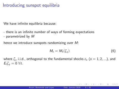
Introducing sunspot equilibria

We have infinite equilibria because:

- there is an infinite number of ways of forming expectations- parametrized by M

hence we introduce sunspots randomizing over M:

Mt = Mt (ζt ) (6)

where ζt i.i.d., orthogonal to the fundamental shocks εs (s = 1, 2, ...), andEtζt = 0 ∀t.

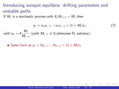
Introducing sunspot equilibria: drifting parameters andunstable pathsIf Mt is a stochastic process with EtMt+1 = Mt then

yt = αtyt−1 − αt εt−1 + (1+Mt )εt (7)

with αt = θMt

Mt−1(with Mt−1 6= 0 otherwise FL solution).

Same form as yt = θyt−1 − θεt−1 + (1+M)εt

Drifting parameters and stochastic volatility within the rationalexpectations framework. Cogley and Sargent (2005), Primiceri(2005).

Intuition:agents can modify in every period the expectation formationprocess

Reconsidering unstable paths: |θ| > 1 and Mt temporarily differentfrom zero

yt = αtyt−1 − αt εt−1 + (1+Mt )εt (7)

with αt = θMt

yt = αtyt−1 − αt εt−1 + (1+Mt )εt (7)

with αt = θMt

yt = αtyt−1 − αt εt−1 + (1+Mt )εt (7)

with αt = θMt

Which process for M? RE Solutions

- With Mt random variable the forecast error becomes:

ηt = (1+Mt )εt + (Mt −Mt−1)

(t−1∑i=1

θi εt−i

- Under RE Et−1ηt = 0, then:

1 Et−1(Mt ) = Mt−1 (Mt martingale)2 Et−1 [(1+Mt )εt ] = 0, (Mt must be uncorrelated with εt)

if |θ| < 1 : Use conditions 1 and 2if |θ| > 1 : Unstable paths. Consider the role of transversality condition

Temporarily explosive paths

All the paths corresponding to expected temporary deviations of Mt

from 0 will not violate the transversality condition

RE requires Mt martingale, butif |θ| > 1 and Mt martingale, when Mt 6= 0 the economy is expectedto remain on the unstable path, so transversality condition would beviolated

=> To allow for temporary unstable paths relax the martingaleassumption (and RE)Deviation can be minimal without practical implications Mprocess

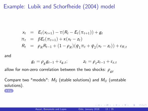
Example: Lubik and Schorfheide (2004) model

xt = Et (xt+1)− τ(Rt − Et (πt+1)) + gtπt = βEt (πt+1) + κ(xt − zt )Rt = ρRRt−1 + (1− ρR )(ψ1πt + ψ2(xt − zt )) + εR ,t

andgt = ρggt−1 + εg ,t ; zt = ρzzt−1 + εz ,t

allow for non-zero correlation between the two shocks: ρgz

Compare two "models": MS (stable solutions) and MU (unstablesolutions).Eig

The estimation strategy

The model has stochastic volatility, then the likelihood distribution isnot Gaussian

Common practice in non linear DSGE literature: use particle filter toapproximate the likelihood in MCMC (Fernandez-Villaverde andRubio-Ramirez, 2007)

Different approach: Particle filter to approximate the posteriordistribution of the parameters and Mt

Sequential Learning on the parameters: how inference evolves overtime gives additional information about the role of sunspots andunstable paths

Particle filter

1 Marginalization. l : all latent states different from M; y : data

p(l ,M |y) = p(l |y ,M)︸︷︷︸Kalman Filter

p(M |y)︸︷︷︸Particle Filter

2 Parameter learning, combining:

1 Particle Learning by Carvalho, Johannes, Lopes and Polson (2010):

2 Liu and West (2001)

See also Chen, Petralia and Lopes (2010)

Priors and Distributions: same as in LS

Models

Estimates Great Inflation sample

Stable Model, Great Inflation:Estimated path for Mt and sequential inference on the parameter ψ1.

Indeterminacy plays a role from the mid 70’Ascari, Bonomolo and Lopes Oslo, January 2018 18 / 35

Unstable Model, Great Inflation

The behavior of Mt

IRFs Models

Comparing the relative fit of Ms/Mu

Cumulative Bayes Factor: 2 ln(Wt ) and the inflation rate

The Bayes Factor strongly favours the unstable modelAscari, Bonomolo and Lopes Oslo, January 2018 20 / 35

Estimates Great Moderation sample

Unstable Model, Great InflationEstimated path for Mt and sequential inference on the parameter γ.

Model MU selects the unique stable solution Models

Comparing the relative fit of Ms/Mu

Cumulative Bayes Factor: 2 ln(Wt ) and the inflation rate

Conclusions

We broaden the class of solutions to linear models

Drifting parameters and stochastic volatility

Temporary unstable paths

Our methodology allows the data to choose between different possiblealternatives: determinacy, indeterminacy and instability

When the data are allowed this possibility, they unambiguously selectthe unstable model to explain the stagflation period in the ‘70s

Temporary unstable paths can be empirically relevant and shouldnot be excluded a priori

Conclusions

Which process for M? Temporary unstable paths

To guarantee the transversality condition relax the martingale assumption(and RE):

Mt = NtAt−1

- Nt martingale- At ∈ {0, 1} non increasing random sequence

Indicate with T̄ random variable: T̄ = inf {t : At = 0}Properties of Mt :

1 Et (Mt+1) = Mt for t < T̄ and t > T̄Et (Mt+1) = 0 for t = T̄

In general Et (ηt+1) = 0.

2 limh→∞ EtMt+h = 0

The transversality condition holds backl

Compare two "models": MS (stable solutions) and MU (unstablesolutions).

Assumption on M

UNDER STABILITY MS

If Taylor principle respected (determinacy) => Mt = 0 ∀tIf Taylor principle not respected (indeterminacy): Mt = Mt−1 + ζt

UNDER INSTABILITY MU

Mt = NtAt−1

Nt ={Nt−1/γ+ ζt with probability γ0 with probability 1− γ

Model MuGI MuGM priors

Transmission mechanism of structural shocks: GIRF in the MU model

Transmission mechanism of sunspot shock: GIRF in the MU model:solid line: M = 0, dashed line: M = 0.52

Rational Sunspots - Norges Bank

Documents

Transcript of Rational Sunspots - Norges Bank