
Rational Krylov subspace methods for phi-functions in ...
143
Rational Krylov subspace methods for ϕ-functions in exponential integrators Zur Erlangung des akademischen Grades eines DOKTORS DER NATURWISSENSCHAFTEN von der Fakult¨ at f¨ ur Mathematik des Karlsruher Instituts f¨ ur Technologie (KIT) genehmigte DISSERTATION von Tanja G¨ ockler ausL¨orrach Tag der m¨ undlichen Pr¨ ufung: 23. Juli 2014 Referent: PD Dr. Volker Grimm 1. Korreferentin: Prof. Dr. Marlis Hochbruck 2. Korreferent: Prof. Dr. habil. Bernhard Beckermann
Transcript of Rational Krylov subspace methods for phi-functions in ...

Rational Krylov subspace methods forϕ-functions in exponential integrators
Zur Erlangung des akademischen Grades eines
DOKTORS DER NATURWISSENSCHAFTEN
von der Fakultat fur Mathematik des
Karlsruher Instituts fur Technologie (KIT)
genehmigte
DISSERTATION
von
Tanja Gockler
aus Lorrach
Tag der mundlichen Prufung: 23. Juli 2014
Referent: PD Dr. Volker Grimm
1. Korreferentin: Prof. Dr. Marlis Hochbruck
2. Korreferent: Prof. Dr. habil. Bernhard Beckermann

Acknowledgements
At this point, I wish to convey my genuine gratitude to a number of people whose supportmade this thesis possible.
First of all, I would like to express my special appreciation and thanks to my advisorPD Dr. Volker Grimm for the opportunity to work on this interesting topic and for hisexcellent supervision, constant support and motivation as well as for countless hours ofhelpful inspiring discussions during the research and writing process of this thesis. I amalso very grateful to Prof. Dr. Marlis Hochbruck for being my second advisor and forgiving me numerous valuable and constructive suggestions. Prof. Dr. habil. BernhardBeckermann from University Lille in France deserves my honest thanks for serving as anexternal referee and for his very useful proposals for improvement.
I thank the Deutsche Forschungsgemeinschaft (DFG) for supporting this work via GR3787 / 1-1.
Moreover, I would like to thank my colleagues for the pleasant and fantastic workingenvironment. A very special thank goes to Lena Martin for careful proofreading andmany helpful suggestions for improvement of my dissertation. In addition, I am obligedto PD Dr. Markus Neher who convinced me to start a doctorate after my first stateexamination and proof-read parts of this thesis. I also acknowledge my friends for theirhelp and encouragement during the period of my PhD studies.
Finally, I extend my sincere gratitude to my family for their invaluable and kind support.


Contents
Notation 3
1 Introduction 5
1.1 Motivation . . . . . . . . . . . . . . . . . . . . . . . . . . . . . . . . . . . . 5
1.2 Outline . . . . . . . . . . . . . . . . . . . . . . . . . . . . . . . . . . . . . . 8
2 Matrix functions 11
2.1 Jordan canonical form . . . . . . . . . . . . . . . . . . . . . . . . . . . . . . 11
2.2 Polynomial interpolation . . . . . . . . . . . . . . . . . . . . . . . . . . . . . 13
2.3 Cauchy integral formula . . . . . . . . . . . . . . . . . . . . . . . . . . . . . 16
3 Discretized evolution equations and exponential integrators 19
3.1 Spatial discretization . . . . . . . . . . . . . . . . . . . . . . . . . . . . . . . 20
3.1.1 Finite differences . . . . . . . . . . . . . . . . . . . . . . . . . . . . . 20
3.1.2 Finite elements . . . . . . . . . . . . . . . . . . . . . . . . . . . . . . 23
3.1.3 Spectral methods . . . . . . . . . . . . . . . . . . . . . . . . . . . . . 26
3.2 Strongly continuous semigroups . . . . . . . . . . . . . . . . . . . . . . . . . 27
3.3 Exponential Runge-Kutta methods . . . . . . . . . . . . . . . . . . . . . . . 31
4 Krylov subspace methods 35
4.1 Orthogonal projections . . . . . . . . . . . . . . . . . . . . . . . . . . . . . . 35
4.2 Standard Krylov subspace . . . . . . . . . . . . . . . . . . . . . . . . . . . . 37
4.3 Rational Krylov subspace . . . . . . . . . . . . . . . . . . . . . . . . . . . . 43
4.4 Near-optimality of the Krylov subspace approximation . . . . . . . . . . . . 50
4.5 Generalization and computation of the Krylov subspace approximation . . . 52
5 Shift-and-invert Krylov subspace approximation 55
5.1 Transformation to the unit disk . . . . . . . . . . . . . . . . . . . . . . . . . 56
5.2 Error bounds for f ∈M . . . . . . . . . . . . . . . . . . . . . . . . . . . . . 61
5.3 Error bounds for the ϕ-functions . . . . . . . . . . . . . . . . . . . . . . . . 63
5.4 Choice of the shift γ . . . . . . . . . . . . . . . . . . . . . . . . . . . . . . . 66
5.5 The case of operators . . . . . . . . . . . . . . . . . . . . . . . . . . . . . . . 69
5.6 Numerical experiments . . . . . . . . . . . . . . . . . . . . . . . . . . . . . . 71
5.6.1 Test example . . . . . . . . . . . . . . . . . . . . . . . . . . . . . . . 71
5.6.2 One-dimensional wave equation . . . . . . . . . . . . . . . . . . . . . 72
5.6.3 Convection-diffusion equation . . . . . . . . . . . . . . . . . . . . . . 75
6 Extended Krylov subspace approximation 81
6.1 Smoothness of the initial value . . . . . . . . . . . . . . . . . . . . . . . . . 82
6.2 Motivation . . . . . . . . . . . . . . . . . . . . . . . . . . . . . . . . . . . . 83
6.3 Error bounds . . . . . . . . . . . . . . . . . . . . . . . . . . . . . . . . . . . 88
6.4 Computation of the extended Krylov subspace approximation . . . . . . . . 93

2 Contents
6.5 Numerical experiments . . . . . . . . . . . . . . . . . . . . . . . . . . . . . . 956.5.1 Schrodinger equation . . . . . . . . . . . . . . . . . . . . . . . . . . . 956.5.2 Wave equation on a non standard domain . . . . . . . . . . . . . . . 102
7 Rational Krylov subspace approximation with simple poles 1117.1 Preliminary notes . . . . . . . . . . . . . . . . . . . . . . . . . . . . . . . . . 1117.2 Error bounds . . . . . . . . . . . . . . . . . . . . . . . . . . . . . . . . . . . 1157.3 Choice of the parameters γ and h . . . . . . . . . . . . . . . . . . . . . . . . 1217.4 Comparison with a fixed rational approximation . . . . . . . . . . . . . . . 1247.5 Numerical experiments . . . . . . . . . . . . . . . . . . . . . . . . . . . . . . 126
7.5.1 Comparison with the fixed rational approximation . . . . . . . . . . 1277.5.2 Convergence rate testing . . . . . . . . . . . . . . . . . . . . . . . . . 1277.5.3 Parallel test example . . . . . . . . . . . . . . . . . . . . . . . . . . . 1287.5.4 Wave equation on a non standard domain . . . . . . . . . . . . . . . 131
8 Conclusion and outlook 133
Bibliography 135

Notation
We always denote matrices with bold capital letters A,B, . . . and vectors with bold smallletters v,w, . . . . Linear operators are designated by capital letters A,B, . . . and functionsby small letters f, g, v, . . . .
I identity matrix
O zero matrix
0 zero vector
Pm space of polynomials with degree less than or equal to m
Pm−1
qm−1
pm−1(z)qm−1(z) : pm−1 ∈ Pm−1
for a fixed qm−1 ∈ Pm−1
diag( · · · ) diagonal matrix
tridiag( · · · ) tridiagonal matrix
pminA minimal polynomial of the matrix A
pminA,v minimal polynomial of A with respect to the vector v
deg(p) degree of the polynomial p
int(Γ) interior of the closed contour Γ
(· , ·) inner product
‖ · ‖ operator, matrix, or vector norm
‖ · ‖2 Euclidean vector norm
‖ · ‖M ‖M1/2 · ‖2, where M is some positive definite Hermitian matrix
σ(A) set of eigenvalues of A
W (A) field of values of A given by (Ax,x) : ‖x‖ = 1C−0 closed left complex half-plane z ∈ C : Re(z) ≤ 0R+
0 real numbers greater than or equal to zero
⊗ Kronecker product
∆, ∇ Laplace and Nabla operator
∇n normal derivative
u′ derivative of u with respect to the time t
∂Ω boundary of the domain Ω
O(·) Landau notation for asymptotic behavior(f(z) = O
(g(z)
)as z → ξ means that there exist constants C, ε > 0
with |f(z)| ≤ C|g(z)| for |z − ξ| < ε)
Cn(Ω) space of n-times continuously differentiable functions on Ω
L1(Ω) space of Lebesgue integrable functions on Ω

L2(Ω) space of quadratically Lebesgue integrable functions on Ω
C∞c (Ω) space of infinitely differentiable functions with compact support on Ω
Hk(Ω) Sobolev space of k-times weakly differentiable L2-functions on Ω
H10 (Ω) closure of C∞c (Ω) in H1(Ω)
I identity operator
T (t) strongly continuous semigroup
D(A) domain of the operator A
ρ(A), σ(A) resolvent set and spectrum of A
Range(A) image of A
Null(A) null space of A
AH complex conjugate transpose of the matrix A
Vm+ Moore-Penrose inverse of Vm
Km(A,v) polynomial Krylov subspace
Qm(A,v) rational Krylov subspace
Kγq+1,m(A,v) extended Krylov subspace
Rm(A) rational matrix subspace
span· · · set of all linear combinations of the vectors in brackets
dim(·) dimension of the space
D, D open and closed unit disk
T interval [−π, π) (real numbers modulo 2π)
ω(g, δ) modulus of continuity defined as sup|s−t|≤δ |g(s)− g(t)|ωr(· , ·) rth modulus of smoothness
ωrφ(· , ·) weighted φ-modulus of smoothness
Tm set of real trigonometric polynomials of degree m
bxc largest integer not greater than x
Ff Fourier transform of f
Lf Laplace transform of f
BV (X) set of functions with bounded variation on the interval X
VarXf variation of f on the interval X
Var∗Xf variation of a correction f∗ of f
1X indicator function of the interval X

Chapter 1
Introduction
1.1 Motivation
Many problems in science and engineering are modeled by partial differential equations.After a discretization in space, for example, by finite differences, finite elements or pseu-dospectral methods, such problems can be written as a semi-linear system of ordinarydifferential equations
u′(t) = Au(t) + g(t,u(t)
), u(0) = u0 (1.1)
with functions u : R → RN , g : R × RN → RN , and a large sparse discretizationmatrix A ∈ RN×N . The parameter N depends on the chosen space grid. Moreover,u0 ∈ RN denotes the initial value and t is the time parameter. Typically, the nonlinearpart g
(t,u(t)
)is non-stiff and the linear part Au(t) is stiff. As the matrix A in the linear
part of (1.1) usually stems from the discretization of an unbounded linear differentialoperator, the norm of A grows for finer and finer space grids.
There is no precise definition of “stiffness”. In the literature, for instance [33, 36, 51], onecan find various descriptions. On the one hand, stiff ordinary differential equations mightbe characterized by the fact that the eigenvalues λi of the discretization matrix A satisfy
maxi|Re(λi)| min
i|Re(λi)| . (1.2)
On the other hand, we often say that a given problem is stiff, if the use of an explicitnumerical integration scheme requires impractically small time steps to obtain the desiredaccuracy, so that for the efficient integration an implicit method is needed which allowsfor larger time steps, but is more costly. A third possible definition is that stiff problemsmay have fast (stiff) and slowly (non-stiff) varying components. This is, for example, thecase in chemical kinetics, where very fast and slow reactions take place simultaneously.
In this context, the example of the wave equation shows the difficulty of measuring stiffness:For explicit schemes, the Courant-Friedrichs-Lewy (CFL) condition enforces a restrictionof the time step size dependent on the spatial mesh. To overcome this drawback, we thushave to use an implicit time integration method. However, the characterization (1.2) doesnot apply in this case, since the discretization matrix A, corresponding to the first orderformulation of the wave equation, has purely imaginary eigenvalues.
In order to cover these different cases of stiffness, we study problems of the form (1.1) witha matrix A whose field of values W (A) is located somewhere in the closed left complexhalf-plane. More precisely, W (A) is generally widely distributed in the left half-plane andthe norm of A can become arbitrarily large. Roughly speaking, we can denote A as a“stiff” matrix.
6 1 Introduction
Up to now, many numerical time integration schemes have been designed to handle stiffdifferential equations. These include exponential integrators which were developed inthe 1960s and are primarily attributable to Certaine [11], Pope [67], Lawson [50], andNørsett [61]. The idea behind this very important class of integrators is to solve the linearpart Au(t) of the model problem (1.1) exactly by the matrix exponential and to integratethe remaining nonlinear part by an explicit scheme. Here, the so-called ϕ-functions comeinto play, which are closely related to the exponential function. These ϕ-functions aregiven as
ϕ`(z) =
∫ 1
0e(1−θ)z θ`−1
(`− 1)!dθ , ` ≥ 1 .
In the simplest case, we approximate the nonlinearity g(t,u(t)
)by g(0,u0) with u0 = u(0)
and obtain the exponential Euler method
u(τ) ≈ eτAu0 + τϕ1(τA)g(0,u0) , ϕ1(z) =ez − 1
z,
which involves the action of the matrix exponential eτA on u0 and the entire ϕ1-functionevaluated at τA times g(0,u0). If g is constant, the scheme reproduces the exact solution.
Exponential integrators have the great advantage that even if ‖A‖ is large, this does notimply a restriction of the admissible time step size τ in the integration. Furthermore,the error bounds do not depend on ‖A‖ as well. Since, in general, A is a huge matrix,the required matrix functions cannot be computed directly. This is why exponentialintegrators have been regarded as impractical for a long time. But in the last decades,it became apparent that there is hope to overcome this drawback by approximating theoccurring products of matrix functions with vectors in a suitable manner.
One possibility is to project A ∈ RN×N onto a subspace of dimension m N , reducingthe problem to the evaluation of a matrix function for a small m × m - matrix, see forinstance [16, 23, 85]. This is the basic idea of the well-known standard Krylov subspacemethod, where f(A)v is approximated by the action of a polynomial matrix functionon the vector v ∈ RN . Besides the standard Krylov subspace method, rational Krylovsubspace techniques have been studied recently in, e.g., [29–31,46,52,59,60,62,69,84]. Astheir name suggests, these methods are based on a rational approximation.
In order to retain the beneficial properties of exponential integrators, it is crucial andindispensable to approximate the occurring matrix functions in such a way that the ap-proximation quality is independent of ‖A‖. Rational Krylov subspace methods representa very promising approach in this direction: In contrast to the polynomial Krylov method,the convergence of the rational process is independent of ‖A‖. This reveals the rationalKrylov subspace method as the optimal choice for our purposes. The following standardmodel problem illustrates these facts.
We consider the one-dimensional heat equation u′ = ∆u on the interval (0, 1) with ini-tial function u0(x) = x(1 − x) and homogeneous Dirichlet boundary conditions. Thediscretization with finite differences leads to the system of ordinary differential equations
u′(t) = Au(t) , u(0) = u0 , A = (N + 1)2 tridiag(1,−2, 1) ∈ RN×N ,
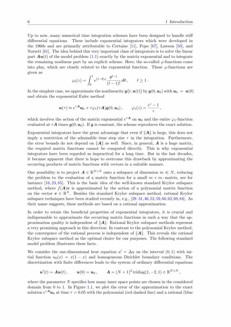
where the parameter N specifies how many inner space points are chosen in the considereddomain from 0 to 1. In Figure 1.1, we plot the error of the approximation to the exactsolution eτAu0 at time τ = 0.05 with the polynomial (red dashed line) and a rational (blue
1.1 Motivation 7
solid line) Krylov subspace method against the number of iteration steps for N = 50 onthe left and N = 200 on the right-hand side. The convergence behavior of the standardKrylov approximation is strongly linked to the number N of inner grid points. The finerthe discretization the later the method starts to converge. The rational Krylov subspaceprocess clearly outperforms the polynomial Krylov approximation and achieves a highaccuracy after only a few iterations independent of the value N .
0 5 10 15 20 2510−14
10−11
10−8
10−5
10−2
N = 50
0 20 40 60 80 10010−14
10−11
10−8
10−5
10−2
N = 200
Figure 1.1: Comparison of the polynomial (red dashed line) and the rational (blue solidline) Krylov subspace method with N = 50, 200 discretization points.
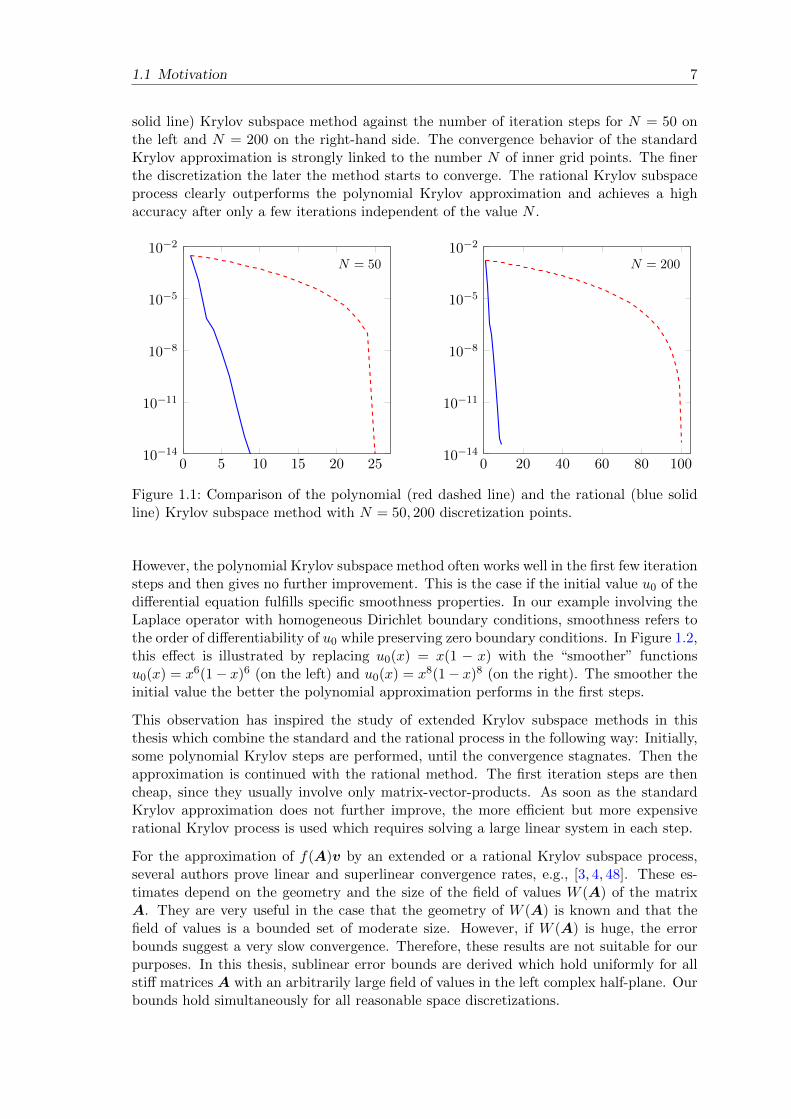
However, the polynomial Krylov subspace method often works well in the first few iterationsteps and then gives no further improvement. This is the case if the initial value u0 of thedifferential equation fulfills specific smoothness properties. In our example involving theLaplace operator with homogeneous Dirichlet boundary conditions, smoothness refers tothe order of differentiability of u0 while preserving zero boundary conditions. In Figure 1.2,this effect is illustrated by replacing u0(x) = x(1 − x) with the “smoother” functionsu0(x) = x6(1− x)6 (on the left) and u0(x) = x8(1− x)8 (on the right). The smoother theinitial value the better the polynomial approximation performs in the first steps.
This observation has inspired the study of extended Krylov subspace methods in thisthesis which combine the standard and the rational process in the following way: Initially,some polynomial Krylov steps are performed, until the convergence stagnates. Then theapproximation is continued with the rational method. The first iteration steps are thencheap, since they usually involve only matrix-vector-products. As soon as the standardKrylov approximation does not further improve, the more efficient but more expensiverational Krylov process is used which requires solving a large linear system in each step.
For the approximation of f(A)v by an extended or a rational Krylov subspace process,several authors prove linear and superlinear convergence rates, e.g., [3, 4, 48]. These es-timates depend on the geometry and the size of the field of values W (A) of the matrixA. They are very useful in the case that the geometry of W (A) is known and that thefield of values is a bounded set of moderate size. However, if W (A) is huge, the errorbounds suggest a very slow convergence. Therefore, these results are not suitable for ourpurposes. In this thesis, sublinear error bounds are derived which hold uniformly for allstiff matrices A with an arbitrarily large field of values in the left complex half-plane. Ourbounds hold simultaneously for all reasonable space discretizations.
8 1 Introduction
0 2 4 6 8 1010−14
10−11
10−8
10−5
10−2
0 2 4 6 8 1010−14
10−11
10−8
10−5
10−2
Figure 1.2: Convergence of the polynomial (red dashed line) and the rational (blue solidline) Krylov subspace approximation for the initial values u0(x) = x6(1 − x)6 (left) andu0(x) = x8(1− x)8 (right).
1.2 Outline
The aim of this thesis is to analyze the convergence of rational and extended Krylovsubspace methods for the approximation of the product of the matrix ϕ-functions and avector, ϕ(A)v, appearing in exponential integrators. With regard to semi-linear problemsof the form (1.1) with stiff linear part, we are interested in error bounds that hold uniformlyfor all matrices A ∈ CN×N with field of values in the closed left complex half-plane. Thatmeans we are searching for convergence rates which are independent of the refinement ofthe spatial discretization.
In Chapter 2, we define matrix functions via the Jordan canonical form, polynomial in-terpolation and the Cauchy integral formula. Moreover, we give a brief overview of somefundamental properties of matrix functions.
The basic concepts and ideas of spatial discretization methods, strongly continuous semi-groups and exponential integrators, especially exponential Runge-Kutta methods, are re-viewed in Chapter 3.
Chapter 4 contains a description of standard and general rational Krylov subspaces aswell as the approximation methods derived from these subspaces. In addition, the near-optimality property of Krylov subspace methods and the efficient computation of theapproximation are discussed.
In the subsequent Chapter 5, a special class of rational Krylov subspace methods is intro-duced, namely the shift-and-invert Krylov subspace approximation, which uses one singlerepeated pole at γ > 0. We derive error bounds for a special class of functions and, inparticular, for the ϕ-functions. Furthermore, suitable choices of γ are suggested.
A convergence analysis of the extended Krylov subspace approximation, whose conver-gence strongly depends on the abstract smoothness of the initial value, is presented inChapter 6.

1.2 Outline 9
In Chapter 7, we turn to the approximation of matrix functions times a vector in a rationalKrylov subspace with different simple poles, which are equidistantly distributed on a linein the right complex half-plane parallel to the imaginary axis.
All results obtained in Chapter 5, 6, and 7 are illustrated by several numerical experimentsat the end of each chapter.
Finally, we give a short conclusion and a brief outlook in Chapter 8.


Chapter 2
Matrix functions
Based on the books [38] by Higham and [47] by Horn and Johnson, we give a brief overviewon the theory of matrix functions in this chapter. The emphasis is placed on the differentdefinitions of matrix functions, as needed for the numerical solution of ordinary or semi-discretized differential equations.
The most familiar matrix function is presumably the matrix exponential that can be usedto express the solution of the homogeneous system
u′(t) = Au(t) , u(0) = u0
by the formula u(t) = etAu0, where A is a constant matrix, whose entries do not dependon the time t. The probably most obvious definition of the matrix exponential etA is givenby the well-known power series
etA =
∞∑k=0
1
k!tkAk ,
which converges for all matrices A, since we have
‖etA‖ ≤∞∑k=0
1
k!tk‖A‖k = et‖A‖ <∞
for any sub-multiplicative matrix norm ‖ · ‖. This is just one of many possibilities forthe computation of etA. In the review [58] by Moler and Van Loan, the authors presenttwenty different ways to compute the exponential of a matrix.
For a general complex-valued function f and an arbitrary square matrix A ∈ CN×N , thereare several more or less equivalent ways to define a matrix function f(A). In the following,we will confine ourselves to the three most important representations determined in termsof the Jordan canonical form, a Hermite interpolation polynomial as well as the Cauchyintegral formula. We will see that the definition of f(A) and its well-definedness arestrongly related to the spectrum σ(A) of A, which is given by
σ(A) := λ ∈ C : λ eigenvalue of A .
Moreover, it will turn out that every matrix function f(A) can be represented pointwise,that means for a fixed matrix A, as a polynomial matrix function.
2.1 Jordan canonical form
Before we address the question of how a general function f : C→ C can be extended to amapping from CN×N to CN×N , we consider the simple case of a polynomial p ∈ Pm, where

12 2 Matrix functions
Pm denotes the set of all polynomials with degree less than or equal to m. In this case, thepolynomial function of a matrix A is defined by inserting A into the given polynomial.
Definition 2.1 For p(z) = amzm + am−1z
m−1 + . . . + a1z + a0 ∈ Pm with z ∈ C andcoefficients a0, . . . , am ∈ C, the polynomial matrix function p(A) is defined as
p(A) := amAm + am−1A
m−1 + . . .+ a1A+ a0I .
It is well-known that every matrix A ∈ CN×N can be represented in Jordan canonicalform
A = SJS−1, J = diag(Jn1 , . . . ,Jns) ,
where n1 + . . . + ns = N , S ∈ CN×N is nonsingular, and J ∈ CN×N is unique up to apermutation of the Jordan blocks Jn1 , . . . ,Jns . Each Jordan block is of the form
Jnk = Jnk(λk) =
λk 1
λk. . .. . . 1
λk
∈ Cnk×nk ,
where the values λk are eigenvalues of the matrix A, which are not necessarily distinct.By inserting A = SJS−1 into a polynomial p, we find
p(A) = Sp(J)S−1, p(J) = diag(p(Jn1), . . . , p(Jns)
).
Using the Taylor expansion
p(z) =
m∑j=0
p(j)(λk)
j!(z − λk)j
around the eigenvalue λk ∈ σ(A) and writing Jnk(λk) = λkI + N , with the nilpotentmatrix N = Jnk(0), we obtain
p(Jnk) =m∑j=0
p(j)(λk)
j!(λkI +N − λkI)j =
minm,nk−1∑j=0
p(j)(λk)
j!N j ,
since N j = O for j ≥ nk. Due to the special structure of N , the matrix N j has the valueone on the jth upper diagonal and zeros elsewhere, and it follows that
p(Jnk) =
p(λk) p′(λk) · · ·
p(nk−1)(λk)
(nk − 1)!
p(λk). . .
.... . . p′(λk)
p(λk)
∈ Cnk×nk .
This shows that p(A) is essentially determined by the derivatives of p(z) at the eigenvaluesof the matrix A. It seems reasonable to generalize the definition of polynomial matrixfunctions p(A) to arbitrary matrix functions f(A). Therefore, we have to ensure that therequired derivatives of f exist on σ(A).

2.2 Polynomial interpolation 13
We recall that the minimal polynomial pminA (z) of A is the unique monic polynomial of
smallest degree such that pminA (A) = O. If we assume that A ∈ CN×N has r distinct
eigenvalues λ1, . . . , λr, this polynomial is given as
pminA (z) =
∏λk∈σ(A)
(z − λk)mk =r∏
k=1
(z − λk)mk , (2.1)
where the exponent mk corresponds to the size of the largest Jordan block associated withthe eigenvalue λk ∈ σ(A). The minimal polynomial is a divisor of any other polynomial pwith p(A) = O.
Definition 2.2 Let pminA , as in (2.1), be the minimal polynomial of A. A function f is
said to be defined on the spectrum σ(A) of A, if f (j)(λk) exists for j = 0, . . . ,mk − 1 andk = 1, . . . , r.
With these considerations in mind, we can state the next definition.
Definition 2.3 Let f be defined on σ(A) and let A = SJS−1 be the Jordan canonicalform of A with J = diag(Jn1 , . . . ,Jns) and Jnk = Jnk(λk) ∈ Cnk×nk . Then we set
f(A) := Sf(J)S−1 = S diag(f(Jn1), . . . , f(Jns)
)S−1 ,
where
f(Jnk) =
f(λk) f ′(λk) · · · f (nk−1)(λk)
(nk − 1)!
f(λk). . .
.... . . f ′(λk)
f(λk)
∈ Cnk×nk . (2.2)
The matrix function f(A) according to Definition 2.3 is well defined, that is, the defini-tion does not depend on the particular Jordan canonical form (Horn and Johnson [47],Theorem 6.2.9). For a diagonalizable matrix A, the blocks f(Jnk) are all of size one, andDefinition 2.3 yields
f(A) = S diag(f(λ1), . . . , f(λN )
)S−1 , J = diag(λ1, . . . , λN ) .
In the case of multi-valued complex functions, such as the square root or the logarithm,it is common practice to use a single branch for the function f in each Jordan block, ifan eigenvalue occurs in more than one block. These matrix functions are called primary.Taking distinct branches for the same eigenvalue in different Jordan blocks, a nonprimarymatrix function is obtained. In this thesis, we will be only concerned with primary matrixfunctions.
2.2 Polynomial interpolation
A further representation of the matrix function f(A) is based on polynomial interpolation.We assume again that λ1, . . . , λr are the distinct eigenvalues of the matrixA ∈ CN×N . Thefirst lemma of this section shows that a matrix polynomial p(A) is completely determinedby the values of p on the spectrum of A.

14 2 Matrix functions
Lemma 2.4 Let pminA (z) = (z − λ1)m1 · · · (z − λr)mr be the minimal polynomial of A and
let p, q be two polynomials. Then we have p(A) = q(A) if and only if
p(j)(λk) = q(j)(λk) for j = 0, . . . ,mk − 1 , k = 1, . . . , r . (2.3)
Proof. Higham [38], Theorem 1.3. o
Lemma 2.4 says that we may replace a given polynomial p in p(A) by an arbitrary poly-nomial q satisfying (2.3) without changing the result. Similar to the considerations in theprevious section, this property can be transferred to general functions. This leads to thefollowing representation of a matrix function via polynomial interpolation.
Theorem 2.5 Let f be defined on σ(A) and let pminA (z) = (z − λ1)m1 · · · (z − λr)
mr
be the minimal polynomial of the matrix A. We have f(A) = p(A) if and only if theν :=
∑rk=1mk = deg(pmin
A ) interpolation conditions
p(j)(λk) = f (j)(λk) for j = 0, . . . ,mk − 1 , k = 1, . . . , r (2.4)
are fulfilled.
Proof. We have to check that the definition of f(A) via the Jordan canonical form inDefinition 2.3 complies with the representation as matrix polynomial p(A), where p has tofulfill the Hermite interpolation condition (2.4). The equivalence of both representationsfollows from the comparison of the individual blocks f(Jnk) defined in (2.2) correspondingto f(A) = Sf(J)S−1 = S diag
(f(Jn1), . . . , f(Jns)
)S−1 and the blocks p(Jnk) corre-
sponding to the polynomial p(A) = S p(J)S−1 = S diag(p(Jn1), . . . , f(Jns)
)S−1. o
By Theorem 2.5, every matrix function f(A) can be written as a polynomial p in A. Theproperties of p depend on the values of the function f and its derivatives on σ(A). Thereexists a uniquely determined polynomial p ∈ Pν−1 with ν = deg(pmin
A ) that satisfies theHermite interpolation condition (2.4). Theorem 2.5 implies further that f(A) and g(A)are equal if and only if
f (j)(λk) = g(j)(λk) for j = 0, . . . ,mk − 1 , k = 1, . . . , r .
An explicit formula for the Hermite interpolation polynomial that fulfills (2.4) is given bythe Lagrange-Hermite formula
p(z) =r∑
k=1
[(mk−1∑j=0
1
j!Φ
(j)k (λk)(z − λk)j
)r∏j=1j 6=k
(z − λj)mj], Φk(z) =
f(z)r∏j=1j 6=k
(z − λj)mj.
If A ∈ CN×N has N distinct eigenvalues, we have mk = 1 for k = 1, . . . , N in the minimalpolynomial and the above formula reduces to the Lagrange interpolation polynomial
p(z) =
N∑k=1
f(λk)
N∏j=1j 6=k
z − λjλk − λj
.

2.2 Polynomial interpolation 15
It is also possible to use divided differences for the computation of the interpolation poly-nomial. For this purpose, we define the tuple
(x1, . . . , xν) := (λ1, . . . , λ1︸ ︷︷ ︸m1
, λ2, . . . , λ2︸ ︷︷ ︸m2
, . . . , λr, . . . , λr︸ ︷︷ ︸mr
)
that contains all distinct eigenvalues λ1, . . . , λr of A according to their multiplicity in theminimal polynomial in the specified order. Then
p(z) =ν∑k=1
f [x1, . . . , xk]k−1∏j=1
(z − xj)
is the desired Hermite interpolation polynomial. For a function f and points xk, . . . , xk+i,the divided differences are given as
f [xk] = f(xk) ,
f [xk, . . . , xk+i] =f [xk+1, . . . , xk+i]− f [xk, . . . , xk+i−1]
xk+i − xkfor xk 6= xk+i ,
f [xk, . . . , xk+i] =f (i)(xk)
i!for xk = xk+i .
Example 2.6 We consider the exponential function f(z) = ez for the matrix
A =
4 1 0 11 1 −1 30 1 4 11 3 −1 1
=
0 2 0 1−1
2 0 1 00 2 0 012 0 1 0
·−2 0 0 00 4 1 00 0 4 10 0 0 4
·
0 2 0 1−1
2 0 1 00 2 0 012 0 1 0
−1
= SJS−1
with minimal polynomial pminA (z) = (z + 2)(z − 4)3. The corresponding Hermite interpo-
lation polynomial that fulfills the required conditions p(−2) = f(−2), p(j)(4) = f (j)(4) forj = 0, 1, 2 is given by
p(z) = e4 + e4(z − 4) +1
2e4(z − 4)2 +
13e4 − e−2
216(z − 4)3
=13e4 − e−2
216z3 − 4e4 − e−2
18z2 − e4 + 2e−2
9z +
31e4 + 8e−2
27.
By construction, we have f(A) = p(A) such that the matrix exponential eA can becomputed by inserting A into the polynomial p. Alternatively, one can use Definition 2.3to obtain
eA = S
f(−2) 0 0 0
0 f(4) f ′(4) 12f′′(4)
0 0 f(4) f ′(4)
0 0 0 f(4)
S−1 =
2e4 e4 −e4 e4
e4 e4+e−2
2 −e4 e4−e−2
2
e4 e4 0 e4
e4 e4−e−2
2 −e4 e4+e−2
2
.The exponential function is depicted in Figure 2.1 together with the associated Hermiteinterpolation polynomial p and its first two derivatives. m
Some useful properties of matrix functions are collected in the following theorem, whichcan be found as Theorem 1.13 in Higham [38]. The proof relies on the representation off(A) via polynomial interpolation.

16 2 Matrix functions
−2 2 4
−40
−20
20
40
60
ez
p(z)
p′(z)
p′′(z)
Figure 2.1: The exponential function and its Hermite interpolation polynomial p corre-sponding to the matrix A.
Theorem 2.7 Let the function f be defined on σ(A), then
1. f(A) and A commute with each other,
2. f(AT ) = f(A)T ,
3. for invertible X, we have f(XAX−1) = Xf(A)X−1,
4. f(λk) are the eigenvalues of f(A), where λk are the eigenvalues of A,
5. X commutes with f(A), if X commutes with A.
2.3 Cauchy integral formula
A third way of representing the matrix function f(A) is via the Cauchy integral formulafrom complex analysis. The generalization of the Cauchy integral theorem from scalarfunctions to matrix functions gives rise to the following theorem.
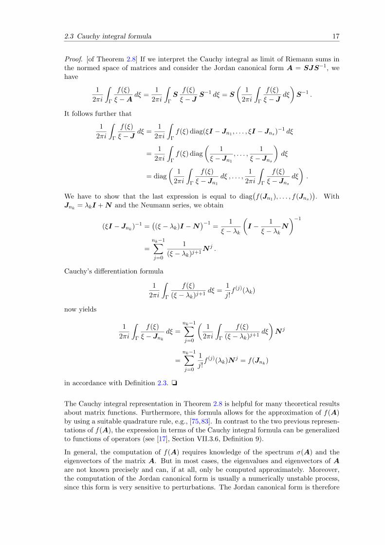
Theorem 2.8 Let f : Ω→ C be analytic in the sim-ply connected domain Ω ⊂ C and let σ(A) ⊂ Ω. Wehave
f(A) =1
2πi
∫Γf(ξ)(ξI −A)−1 dξ ,
where Γ is an arbitrary simple closed rectifiable curvethat encloses σ(A) in Ω and has winding number one.
Ω
Γ
λ1
λ2
λr
For σ(A) ⊂ int(Γ), the curve Γ is disjoint from the spectrum of A and the resolvent(ξI − A)−1 in the integrand is well-defined. The resolvent is a matrix function as well.For better readability, we will often use the short notation 1
ξ−A in the following instead of
the equivalent expression (ξI −A)−1.
2.3 Cauchy integral formula 17
Proof. [of Theorem 2.8] If we interpret the Cauchy integral as limit of Riemann sums inthe normed space of matrices and consider the Jordan canonical form A = SJS−1, wehave
1
2πi
∫Γ
f(ξ)
ξ −Adξ =
1
2πi
∫ΓS
f(ξ)
ξ − JS−1 dξ = S
(1
2πi
∫Γ
f(ξ)
ξ − Jdξ
)S−1 .
It follows further that
1
2πi
∫Γ
f(ξ)
ξ − Jdξ =
1
2πi
∫Γf(ξ) diag(ξI − Jn1 , . . . , ξI − Jns)−1 dξ
=1
2πi
∫Γf(ξ) diag
(1
ξ − Jn1
, . . . ,1
ξ − Jns
)dξ
= diag
(1
2πi
∫Γ
f(ξ)
ξ − Jn1
dξ , . . . ,1
2πi
∫Γ
f(ξ)
ξ − Jnsdξ
).
We have to show that the last expression is equal to diag(f(Jn1), . . . , f(Jns)
). With
Jnk = λkI +N and the Neumann series, we obtain
(ξI − Jnk)−1 =((ξ − λk)I −N
)−1=
1
ξ − λk
(I − 1
ξ − λkN
)−1
=
nk−1∑j=0
1
(ξ − λk)j+1N j .
Cauchy’s differentiation formula
1
2πi
∫Γ
f(ξ)
(ξ − λk)j+1dξ =
1
j!f (j)(λk)
now yields
1
2πi
∫Γ
f(ξ)
ξ − Jnkdξ =
nk−1∑j=0
(1
2πi
∫Γ
f(ξ)
(ξ − λk)j+1dξ
)N j
=
nk−1∑j=0
1
j!f (j)(λk)N
j = f(Jnk)
in accordance with Definition 2.3. o
The Cauchy integral representation in Theorem 2.8 is helpful for many theoretical resultsabout matrix functions. Furthermore, this formula allows for the approximation of f(A)by using a suitable quadrature rule, e.g., [75,83]. In contrast to the two previous represen-tations of f(A), the expression in terms of the Cauchy integral formula can be generalizedto functions of operators (see [17], Section VII.3.6, Definition 9).
In general, the computation of f(A) requires knowledge of the spectrum σ(A) and theeigenvectors of the matrix A. But in most cases, the eigenvalues and eigenvectors of Aare not known precisely and can, if at all, only be computed approximately. Moreover,the computation of the Jordan canonical form is usually a numerically unstable process,since this form is very sensitive to perturbations. The Jordan canonical form is therefore

18 2 Matrix functions
commonly avoided in numerical analysis. Consequently, the representations of f(A) basedon the Jordan canonical form or the corresponding Hermite interpolation polynomial yieldno adequate methods to determine f(A) exactly. The Cauchy integral formula is typicallynot used for the exact computation of f(A) as well.
Hence, one has to carefully design algorithms that compute accurate approximations tomatrix functions for dense matrices of moderate size. This is still a subject of currentresearch. Fortunately, for the matrix exponential and the matrix ϕ-functions, which areof interest in this thesis, algorithms for dense and moderate-sized matrices are known,cf. [2, 38, 77]. An overview about the computation of f(A) for more general functions fand dense matrices A can be found in [38,39].
In view of the numerical solution of differential equations, we are interested in the eval-uation of the action of a matrix function f(A) on a vector v, without computing f(A)explicitly. We will see that Krylov subspace methods are suitable to approximate f(A)vefficiently. Here, the methods for dense matrices cannot be applied. The occurring ma-trices A are sparse and large, but f(A) is usually a large non-sparse matrix. The ideato circumvent the problems mentioned above is to project the large matrix A ∈ CN×Nonto some Krylov subspace of dimension m N . This approach reduces A to a smallermatrix Sm of size m ×m for which f(Sm) can be determined with standard algorithmsfor dense matrices of moderate size. We will come back to this issue in Chapter 4.

Chapter 3
Discretized evolution equations andexponential integrators
We are interested in the time integration of semi-linear problems of the form
u′(t) = Au(t) + g(t, u(t)
), u(0) = u0 , (3.1)
which represents either a system of ordinary differential equations in CN , that stems froma suitable spatial discretization of a partial differential equation, or an abstract evolutionequation on some Banach space with a linear, usually unbounded, differential operatorA. Later on in this thesis, we will often restrict ourselves to Hilbert spaces, which are aspecial case of Banach spaces.
In the first case, we denote by A ∈ CN×N the discretization matrix and by u ∈ CN theapproximation of the exact solution. For a finite-difference discretization, for example, thisvector u contains approximate values of the solution u at certain grid points of the spatialdomain. For a finite-element discretization, u is the coefficient vector of the nodal basisfunctions. In the discrete case, we thus write equation (3.1) as u′(t) = Au(t) +g
(t,u(t)
),
u(0) = u0 with bold letters.
In the second case, one usually has to discretize the operator A by some kind of dis-cretization process, such as finite-difference, pseudospectral, or finite-element methods.Therefore, we are concerned with matrices anyway. Nevertheless, we will study the fol-lowing approximation methods in time for the abstract equation (3.1), in order to gaininsight in the convergence behavior.
In what follows, we will consider stiff problems, where A is an unbounded operator on someHilbert space H, or a huge matrix, whose norm can become arbitrarily large. Stiff dis-cretization matrices A corresponding to the discretization of a partial differential equationmay be characterized by a large field of values
W (A) :=
(Ax,x)
(x,x): x ∈ CN , x 6= 0
= (Ax,x) : x ∈ CN , ‖x‖ = 1
located in the left complex half-plane, i.e., W (A) ⊆ C−0 with
C−0 := z ∈ C : Re(z) ≤ 0 ,
see, for instance, [36,51]. By (· , ·) we always denote a suitable inner product on CN withassociated norm ‖x‖ =
√(x ,x) for x ∈ CN .
As a consequence of their bounded stability region, explicit integrators usually fail to in-tegrate the linear part of (3.1) for stiff problems, unless impractically small time steps areused. Exponential integrators are an important class of numerical methods for the time

20 3 Discretized evolution equations and exponential integrators
integration of evolution equations which overcome this drawback. The name “exponentialintegrators” arises from the fact that these special integrators contain the matrix expo-nential or the operator exponential, i.e., the strongly continuous semigroup generated byA, and so-called ϕ-functions that are closely related to the exponential function.
Before we explain the ideas of exponential integrators and their construction based on thereview [44] by Hochbruck and Ostermann, we outline the spatial discretization of partialdifferential equations, e.g., [9,55]. For fine space discretizations, the discretization matricesare huge and we might say that the matrix exponential corresponds to an approximationof the semigroup. We will need this correspondence later on, in order to understandthe convergence of our methods. Therefore, we will summarize fundamental facts aboutstrongly continuous semigroups and their generators following the books by Miklavcic [57],by Pazy [65], and by Engel and Nagel [19].
3.1 Spatial discretization
Using a spatial discretization, a partial differential equation is transformed into a systemof ordinary differential equations of the form (3.1) with A ∈ CN×N and u ∈ CN . Thissystem of ordinary differential equations can then be solved with the help of standard timeintegration methods. As an example of a stiff system, we consider the two-dimensionalheat equation with homogeneous Dirichlet boundary conditions
u′ = ∆u for (x, y) ∈ Ω , t ≥ 0 ,
u(0, x, y) = u0(x, y) for (x, y) ∈ Ω ,
u(t, x, y) = 0 for (x, y) ∈ ∂Ω , t ≥ 0
on the Hilbert space L2(Ω) for a given domain Ω ⊂ R2. The space L2(Ω) contains allfunctions that are quadratically Lebesgue integrable on Ω, that is,
L2(Ω) := f : Ω→ R :
∫Ω|f |2 d(x, y) <∞ .
Moreover, ∆ denotes the Laplacian ∆ = ∂2
∂x2 + ∂2
∂y2 on R2.
In the following, we will focus on the finite-difference, the finite-element, and the spectraldiscretization, and present the basic ideas of these methods.
3.1.1 Finite differences
As domain Ω, we take a square. For the approximation, we discretize Ω by a uniformgrid with mesh size h = 1
n+1 and equidistant nodes (xi, yj) = (x0 + ih, y0 + jh) ∈ Ω,i, j = 0, . . . , n+ 1, in each direction as depicted in Figure 3.1. If the solution u of the heatequation is sufficiently smooth, Taylor expansion yields
∂2
∂x2u(t, xi, yj) =
1
h2
(u(t, xi + h, yj)− 2u(t, xi, yj) + u(t, xi − h, yj)
)+O(h2) .
The same considerations apply to the second derivative of u with respect to the spacevariable y. Neglecting the remainder term of order h2, which is small for a fine spatial
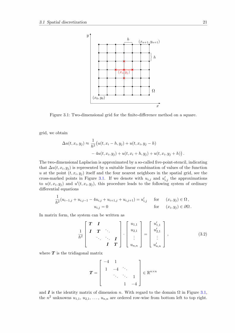
3.1 Spatial discretization 21
x
y
(x0, y0)
(xn+1, yn+1)
(xi, yj)
h
h
Ω
Figure 3.1: Two-dimensional grid for the finite-difference method on a square.
grid, we obtain
∆u(t, xi, yj) ≈1
h2
(u(t, xi − h, yj) + u(t, xi, yj − h)
− 4u(t, xi, yj) + u(t, xi + h, yj) + u(t, xi, yj + h)).
The two-dimensional Laplacian is approximated by a so-called five-point-stencil, indicatingthat ∆u(t, xi, yj) is represented by a suitable linear combination of values of the functionu at the point (t, xi, yj) itself and the four nearest neighbors in the spatial grid, see thecross-marked points in Figure 3.1. If we denote with ui,j and u′i,j the approximationsto u(t, xi, yj) and u′(t, xi, yj), this procedure leads to the following system of ordinarydifferential equations
1
h2(ui−1,j + ui,j−1 − 4ui,j + ui+1,j + ui,j+1) = u′i,j for (xi, yj) ∈ Ω ,
ui,j = 0 for (xi, yj) ∈ ∂Ω .
In matrix form, the system can be written as
1
h2
T I
I T. . .
. . .. . . II T
·u1,1
u2,1
...
un,n
=
u′1,1u′2,1
...
u′n,n
, (3.2)
where T is the tridiagonal matrix
T =
−4 1
1 −4. . .
. . .. . . 1
1 −4
∈ Rn×n
and I is the identity matrix of dimension n. With regard to the domain Ω in Figure 3.1,the n2 unknowns u1,1, u2,1, . . . , un,n are ordered row-wise from bottom left to top right.
22 3 Discretized evolution equations and exponential integrators
This allows to reformulate the considered heat equation as the system
u′(t) = Au(t) , u(0) = u0 ,
where A ∈ RN×N , N = n2, is the block tridiagonal matrix A = tridiag(I,T , I) andu(t) ∈ RN is a vector containing the values u1,1, u2,1, . . . , which are approximations tou(t, x1, y1), u(t, x2, y1), . . . on the inner grid points. A discrete approximation for thesolution u is then determined by solving u′(t) = Au(t) with a time integration methodfor ordinary differential equations, where “discrete” means that the numerical solution isknown only at certain points of the space domain Ω.
To reveal the stiff character of the semi-discrete system u′(t) = Au(t), we compute theeigenvalues of the discretization matrix A. With the help of the Kronecker product ⊗,the matrix A is represented as
A = I ⊗L+L⊗ I, L =1
h2
−2 1
1 −2. . .
. . .. . . 1
1 −2
∈ Rn×n .
The eigenvalues of the tridiagonal matrix L are well-known, cf. [51], Section 2.10. They aregiven by λk = − 4
h2 sin2(
kπ2(n+1)
)for k = 1, . . . , n. For two matrices B and C with eigen-
values µ1, . . . , µn and ν1, . . . , νn, the eigenvalues of the Kronecker product B⊗C are µiνjfor i, j = 1, . . . , n. With the Jordan canonical form L = SJS−1, J = diag(λ1, . . . , λn), itfollows that
I ⊗L+L⊗ I = (S ⊗ S)(I ⊗ J + J ⊗ I)(S ⊗ S)−1
by the properties of the Kronecker product. Since σ(A) = σ(I⊗J+J⊗I), the eigenvaluesof A are given by
− 4
h2
(sin2
(iπ
2(n+ 1)
)+ sin2
(jπ
2(n+ 1)
)), i, j = 1, . . . , n .
For fine discretizations of the domain Ω, the mesh size h becomes small and σ(A) containsnegative eigenvalues of small as well as very large absolute value. This illustrates that weare concerned with a stiff problem.
If we want to measure the quality of the numerical solution u, it is appropriate to scalethe standard Euclidean norm ‖ · ‖2 with the mesh size h of the space grid (e.g., [55],Section 6.1). This scaled Euclidean norm,
‖u‖h := h‖u‖2 =
(h2
n∑i,j=1
u2ij
) 12
≈(∫
Ωu2d(x, y)
) 12
,
can be interpreted as a discrete L2-norm. For an arbitrary matrix A ∈ CN×N , the inducedmatrix norm ‖ · ‖h coincides with the spectral matrix norm ‖ · ‖2, since
‖A‖h = supx6=0
‖Ax‖h‖x‖h
= supx6=0
‖Ax‖2‖x‖2
= ‖A‖2 .
3.1 Spatial discretization 23
3.1.2 Finite elements
In contrast to the finite-difference method, where the exact solution is approximated atcertain grid points, the finite-element method is based on taking an appropriate linearcombination of some fixed nodal basis functions φi on subregions of the space domain Ω,that is,
u(t, x, y) ≈N∑i=1
ui(t)φi(x, y) .
We first state a variational formulation by rewriting our problem in a weak form. Sub-sequently, we discretize the problem with respect to the space variables x and y, which
yields an approximate solution u(t) =(ui(t)
)Ni=1
in the finite-element space SN of dimen-sion N . In the simplest case, this finite-element space contains continuous, piecewise linearfunctions on a partition of the domain Ω containing triangular elements.
By (· , ·)L2(Ω) and ‖ · ‖L2(Ω) we denote the inner product and its induced matrix norm
(v, w)L2(Ω) =
∫Ωvw d(x, y) , ‖v‖L2(Ω) =
√(v, v)L2(Ω) , v, w ∈ L2(Ω) .
We define the Sobolev space
Hk(Ω) := v ∈ L2(Ω) :∂α+β
∂αx ∂βyv(x, y) ∈ L2(Ω) , α+ β ≤ k , α, β ∈ N0 ,
where the derivatives are understood in the weak sense. Moreover, we need the Sobolevspace H1
0 (Ω), which is the closure of C∞0 (Ω) with respect to the Sobolev norm ‖ · ‖H1(Ω).Hereby, C∞0 (Ω) is the space of infinitely differentiable functions on Ω with compact supportand the H1-norm, induced by the inner product
(v, w)H1(Ω) =
∫Ωvw d(x, y) +
∫Ω∇v∇w d(x, y) ,
is given as
‖v‖H1(Ω) =(‖v‖2L2(Ω) + ‖∇v‖2L2(Ω)
) 12,
where ∇v is a weak gradient vector that contains the weak partial derivatives of v. Infact, H1
0 (Ω) contains all functions whose weak derivative belongs to the space L2(Ω) andthat vanish on the boundary ∂Ω of the considered domain Ω.
To find the weak formulation for the heat equation, we multiply the differential equationby a test function φ ∈ H1
0 (Ω), integrate over Ω, and apply Green’s formula such that∫Ωφu′ d(x, y) =
∫Ωφ∆u d(x, y) = −
∫Ω∇φ∇u d(x, y) +
∫∂Ωφ∇nu ds
for all φ ∈ H10 (Ω), where ∇nu designates the normal derivative of u. The integral over ∂Ω
vanishes for φ ∈ H10 (Ω), since by assumption φ is equal to zero on ∂Ω. Using the inner
product on L2(Ω), one can briefly note
(φ, u′)L2(Ω) = −(∇φ,∇u)L2(Ω) .

24 3 Discretized evolution equations and exponential integrators
Let φ1, . . . , φN be a basis of the finite-element space SN . We replace u(t, x, y) by a linearcombination of these basis functions, that is, u(t, x, y) ≈
∑Ni=1 ui(t)φi(x, y) ∈ SN , and
search for coefficients ui(t) such that
N∑i=1
u′i(t)(φi, φk)L2(Ω) = −N∑i=1
ui(t)(∇φi,∇φk)L2(Ω) for k = 1, . . . , N . (3.3)
If we approximate the initial function u0(x, y) by∑N
i=1 γi φi(x, y) ∈ SN , we have ui(0) = γifor i = 1, . . . , N . With the vectors u(t) =
(ui(t)
))Ni=1 and u0 = (γi)
Ni=1, equation (3.3) reads
Mu′(t) = Su(t) , u(0) = u0
in matrix notation, where M is the so-called mass matrix and S the stiffness matrix,whose entries are given by
(M)ij = mij = (φi, φj)L2(Ω) , (S)ij = sij = −(∇φi,∇φj)L2(Ω) , i, j = 1, . . . , N .
The solution of this system can then be approximated by standard methods for ordinaryinitial value problems. The matrix M is symmetric positive definite and thus invertible.Multiplying both sides with M−1 from the left yields the ordinary differential equationu′(t) = M−1Su(t) which has the form (3.1) with the stiff matrix A = M−1S and g = 0 .
We have not yet considered the question of how the nodal basis functions φi look like inour case. The first step consists of generating a suitable triangulation over the domain Ω.First, the given domain is approximated by a polygon ΩT . The triangulation is composedof triangles Ki, i = 1, . . . , E, such that the triangles meet edge-to-edge and vertex-to-vertex and Ω = K1 ∪K2 ∪ . . . ∪KE . We denote by hi the diameter of the circumcircle ofthe triangle Ki and by ρi the radius of the circle inscribed in Ki. We assume that the ratioof hi to ρi is smaller than some constant, so that triangles with very small or large anglesare avoided. In the following, the inner nodes of our mesh are denoted by a1, . . . , aN . Inthe simplest case, we construct piecewise linear basis functions with
φi(aj) =
1 , i = j ,
0 , i 6= jfor i, j = 1, . . . , N ,
so that φi is equal to zero on all triangles that do not contain the vertex ai. Since φi = 0for all i with ai ∈ ∂ΩT , the basis functions are in H1
0 (ΩT ), and moreover form a basis ofthe finite-element space SN .
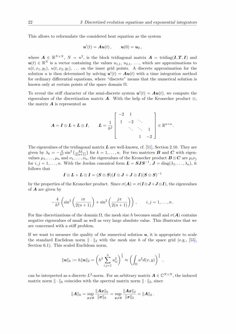
A simple example, where the rectangular domain ΩT is discretized with congruent trian-gles, is shown in Figure 3.2. Additionally, we depict one of the basis functions φi, thattakes the value one at the vertex ai and is equal to zero on all other vertices.
Since mij and sij are only different from zero, if the vertices ai and aj belong to thesame triangle, the mass matrix M and the stiffness matrix S are sparse. This is alsodemonstrated in the following example.
Example 3.1 We take the simple 4×5 - grid with mesh size h and inner vertices a1, . . . , a6,which is shown in Figure 3.3. If we want to compute, e.g., the entry s11 = (∇φ1,∇φ1)L2(Ω)
of the stiffness matrix S, it suffices to consider the six triangles K1, . . . ,K6 adjacent to a1
separately to obtain
s11 = −6∑j=1
∫Kj
∇φ1∇φ1 d(x, y) = −1
2h2
(2
h2+
1
h2+
1
h2+
2
h2+
1
h2+
1
h2
)= −4 .
3.1 Spatial discretization 25
ai
φi
ΩT
Figure 3.2: Basis function φi corresponding to the node ai.
In order to determine s12, we only have to investigate K3 and K4, since ∇φ1∇φ2 is zeroon the other triangles. This yields
s12 = −1
2h2
(− 1
h2− 1
h2
)= 1 .
Similar considerations apply to the remaining entries of the stiffness matrix S. For theentries (M)ij = (φi, φj)L2(Ω), i, j = 1, . . . , 6, of the mass matrix, the computation issimplified by using a quadrature formula. If K is a triangle with area |K| and (xk, yk),k = 1, 2, 3, are the midpoints of the sides, the quadrature rule∫
Kp(x, y) d(x, y) ≈ |K|
3
(p(x1, y1) + p(x2, y2) + p(x3, y3)
)is exact for any quadratic polynomial p. By making use of these facts, one can easilycompute
M = h2 · 1
12
6 1 0 1 0 01 6 1 1 1 00 1 6 0 1 11 1 0 6 1 00 1 1 1 6 10 0 1 0 1 6
, S =
−4 1 0 1 0 01 −4 1 0 1 00 1 −4 0 0 11 0 0 −4 1 00 1 0 1 −4 10 0 1 0 1 −4
.
Note that S has the same structure as the matrix A = I ⊗ L + L ⊗ I from the finite-difference discretization. The eigenvalues of M−1S all lie in the left complex half-plane.Their proportionality to 1
h2 expresses again the stiff character of the heat equation. m
In practical computations, the inner products in the mass and the stiffness matrix, arecomputed in a clever way by an assembling process. We consider the single triangleselement-wise, determine locally the corresponding integrals on each element, and assemblethe derived information. For a fast and effective computation, the triangles are mappedby an affine transformation to a reference element K, and the integration is performed byusing an appropriate quadrature formula.
Analogously to the scaled Euclidean norm ‖ · ‖h = h‖ · ‖2 for the finite-difference method,we have to use a suitable discrete L2-norm. This can be motivated by the equality∫
Ωu2 d(x, y) ≈
N∑i,j=1
ui(t)uj(t) (φi, φj)L2(Ω) = u(t)TMu(t) .

26 3 Discretized evolution equations and exponential integrators
ΩK1
K2
K3
K4
K5
K6
h
a1 a2 a3
a4 a5 a6
Figure 3.3: Regular grid used in Example 3.1.
Since the mass matrixM ∈ RN×N is symmetric and positive definite, there exists a uniquematrix square root M1/2 which is also symmetric positive definite (cf. [26], Section 4.2.4).The matrix M is unitary diagonalizable by M = Q diag(η1, . . . , ηN )QT and the matrixsquare root M1/2 is thus given by Q diag(
√η1, . . . ,
√ηN )QT . For u := u(t) ∈ RN , we
therefore define
‖u‖M =√
(u,u)M , (u,u)M = uTMu = ‖M1/2u‖22 .
For an arbitrary matrix A ∈ CN×N , we then obtain
‖A‖M = supx6=0
‖Ax‖M‖x‖M
= supx6=0
‖M1/2AM−1/2M1/2x‖2‖M1/2x‖2
= ‖M1/2AM−1/2‖2 .
3.1.3 Spectral methods
Later on in this thesis, we will also use a spectral discretization, but only for one-dimensional problems. For this reason, we mention only briefly the idea behind thisdiscretization method. A detailed description is then given within the sections of thecorresponding numerical experiments.
The spectral method is based on approximating the unknown solution u by a finite linearcombination of the eigenfunctions ψj,k(x, y) of the Laplacian with homogeneous Dirichletboundary conditions. For instance, in the special case when Ω = (0, 1)2, these eigenfunc-tions read
ψj,k(x, y) = C · sin(jπx) sin(kπy) , j, k ∈ N ,
where the constant C is chosen such that∫
Ω ψ2j,k d(x, y) = 1. The functions ψj,k form an
orthonormal basis of L2(Ω). Because of
∆ψj,k(x, y) = −π2(j2 + k2)ψj,k(x, y) ,
the corresponding eigenvalues are −π2(j2 + k2) for j, k ∈ N. A discretization is nowobtained by substituting the ansatz
u(t, x, y) ≈n∑
j,k=1
uj,k(t)ψj,k(x, y)

3.2 Strongly continuous semigroups 27
in the given heat equation, which yields
n∑j,k=1
u′j,k(t)ψj,k(x, y) = −n∑
j,k=1
π2(j2 + k2)uj,k(t)ψj,k(x, y) .
This represents a system of ordinary differential equations
u′(t) = Au(t) ,
where u(t) ∈ RN , N = n2, contains the coefficients uj,k(t), that have to be determined.The discretization matrix A ∈ RN×N is a diagonal matrix with entries −π2(j2 + k2) forj, k = 1, . . . , n, and norm ‖A‖2 = 2π2N .
In conclusion of this section, the following can be said: Not only for the heat equation,but also for general abstract or discretized differential equations, we should always keepin mind that we are concerned with unbounded operators or huge discretization matrices,whose norm can become arbitrarily large for very fine grids. In simple terms, one mightsay that the discretization matrix is approaching more and more the associated unboundeddifferential operator, if we refine the spatial grid. With regard to the approximation ofthe matrix exponential and related matrix ϕ-functions in exponential integrators, it willtherefore be decisive to obtain error bounds that are not affected by the unboundednessof the operator A and that do not depend on the norm of the discretization matrix A.
3.2 Strongly continuous semigroups
Let X be some Banach space. We denote by ‖ · ‖ the norm on X as well as the operatornorm that is for a bounded operator B : X → X defined as
‖B‖ = supx∈Xx 6=0
‖Bx‖‖x‖
.
In the following, we are concerned with the abstract semi-linear problem
u′(t) = Au(t) + g(t, u(t)
), u(0) = u0 , (3.1)
where A : D(A) ⊆ X → X is a linear, in general unbounded, operator on X with domainof definition D(A). If g
(t, u(t)
)= 0, (3.1) reduces to
u′(t) = Au(t) , u(0) = u0 . (3.4)
For u0 ∈ D(A), we assume that there exists a unique solution u(t) of (3.4). Then we candefine an operator semigroup T (t) such that
T (t)u0 := u(t) for t ≥ 0 ,
where T (0) = I is the identity on X and the mapping t 7→ T (t)u0 is continuous from R+0
to the Banach space X. If we choose u(s) as initial value, the uniqueness of the solutionimplies that
T (t)u(s) = T (t)T (s)u0 = u(t+ s) = T (t+ s)u0 ,
indicating the semigroup property T (t)T (s) = T (t + s). These fundamental facts are

28 3 Discretized evolution equations and exponential integrators
summarized in the following definition.
Definition 3.2 A family(T (t)
)t≥0
of bounded linear operators on a Banach space X is
called a strongly continuous semigroup (or shortly C0-semigroup), if the following condi-tions are fulfilled:
(a) We have T (t+ s) = T (t)T (s) for all t, s ≥ 0 and T (0) = I.
(b) For every x ∈ X, the orbit map
ξx : R+0 → X , t 7→ T (t)x
is continuous.
It is well-known that right continuity of the orbit map at zero implies continuity ofξx on [0,∞). That is, we can replace part (b) in Definition 3.2 by the requirementlimt0 ‖T (t)x− x‖ = 0 for all x ∈ X. We immediately derive from Definition 3.2 that theoperators commute, since
T (t)T (s) = T (t+ s) = T (s+ t) = T (s)T (t) .
Furthermore, one can easily prove by induction that
T (nt) = T (t+ . . .+ t) = T (t)n for n ∈ N .
By the continuity of the orbit map ξx, it follows that T (t) is locally bounded on compactintervals [0, t0], that is ‖T (t)x‖ <∞ for all t ∈ [0, t0], t0 > 0, and every x ∈ X. From theUniform Boundedness Principle1, we conclude that a C0-semigroup is uniformly boundedon each compact interval of R+
0 . This fact implies that every strongly continuous semigroupis exponentially bounded. More exactly, there exist constants M ≥ 1 and ω ≥ 0 such thatthe inequality
‖T (t)‖ ≤Meωt for all t ≥ 0 (3.5)
holds true. To see this, we choose t0 > 0 and M ≥ 1 with ‖T (s)‖ ≤ M for all s ∈ [0, t0]and set t = s+ nt0 for n ∈ N0. Then
‖T (t)‖ ≤ ‖T (s)‖‖T (t0)‖n ≤Mn+1 ≤Meωnt0 ≤Meωt for all t ≥ 0 ,
where ω = ln(M)/t0 ≥ 0. If the semigroup satisfies inequality (3.5), we also say that T (t)is of type (M,ω). At this point, it should be noted that there are also semigroups whichsatisfy (3.5) with ω < 0.
Since T (t)u0 can be regarded as the unique solution of the abstract equation (3.4) withinitial value u0, we should analyze strongly continuous semigroups with respect to theirdifferentiability. First, we point out that right differentiability of the orbit map ξx at t = 0is equivalent to differentiability of ξx on R+
0 . Its derivative is given by
ξ′x(t) = T (t) ξ′x(0) for all t ≥ 0 .
The right derivative ξ′x(0) at t = 0 yields an operator A that is called the infinitesimalgenerator of the C0-semigroup.
1Uniform Boundedness Principle: If a set T of bounded linear operators is pointwise bounded, then it isuniformly bounded (e.g., Theorem 3.17 in [74]).

3.2 Strongly continuous semigroups 29
Definition 3.3 The infinitesimal generator (or simply generator) A : D(A) ⊆ X → X ofa strongly continuous semigroup
(T (t)
)t≥0
is defined as
Ax := ξ′x(0) =d
dtT (t)x
∣∣∣t=0
= limh0
1
h
(T (h)x− x
)for every x in the domain
D(A) := x ∈ X : limh0
1
h
(T (h)x− x
)exists . (3.6)
The following example illustrates that every matrix A ∈ CN×N generates, as a specialcase of a linear operator on CN , a C0-semigroup. In analogy to the matrix exponential, itprovides a motivation to think of the semigroup T (t) as an operator exponential etA. Forthis reason, we will also write etA for T (t).
Example 3.4 We consider a matrix A ∈ CN×N on X = CN . It is well known that thesolution of the initial value problem u′(t) = Au(t), u(0) = u0, is given by
T (t)u0 := etAu0 , t ∈ R .
One can easily check that etA satisfies the semigroup properties and that ddt e
tA = AetA
for all t ∈ R. Consequently, T (t) is not only a C0-semigroup, but moreover a C0-group(i.e., Definition 3.2 holds for t ∈ R) with infinitesimal generator A. If the field of valuesW (A) is contained in the left complex half-plane, the semigroup is bounded by one, thatis, ‖etA‖ ≤ 1 with M = 1 and ω = 0 in (3.5), cf. Lemma 7.1 below. Such semigroups oftype (1, 0) are called contraction semigroups. m
It follows directly from the definition that the generator A of a strongly continuous semi-group T (t) is a linear operator. Another important property is that the C0-semigroup andits generator commute on D(A). If x ∈ D(A), then also T (t)x ∈ D(A) and
d
dtT (t)x = T (t)Ax = AT (t)x for all t ≥ 0 .
The infinitesimal generator A is a closed and densely defined operator that determines thesemigroup uniquely. Closedness means that xn → x and Axn → y in X for any sequence(xn)n∈N in D(A) implies x ∈ D(A) and Ax = y. An operator A is called densely defined,if its domain D(A) is dense in X.
It is also important to look at the spectral properties of the generator A. For this purpose,we recall the following definition.
Definition 3.5 The resolvent set of a closed linear operator A : D(A) ⊆ X → X isdefined by
ρ(A) := z ∈ C : zI −A is bijective .The spectrum of A is given as σ(A) := C \ ρ(A).
Assuming z ∈ ρ(A), the inverse R(z,A) := (zI−A)−1 exists. It is also called the resolventof A. If A is closed, the resolvent R(z,A) is closed as well. By definition, the domain ofR(z,A) is equal to X and we can conclude from the Closed Graph Theorem2 that
R(z,A) : X → D(A) , z ∈ ρ(A)
2Closed Graph Theorem: If X, Y are Banach spaces and B : D(B) ⊆ X → Y is a closed linear operatorwith D(B) = X, then B is bounded (e.g., Theorem 3.10 in [74]).

30 3 Discretized evolution equations and exponential integrators
is a bounded operator on X. Furthermore, we have the identity
zR(z,A)− I = AR(z,A) , z ∈ ρ(A)
and, for all x ∈ D(A), the resolvent commutes with A, i.e., AR(z,A)x = R(z,A)Ax. Themapping z 7→ R(z,A), z ∈ ρ(A), is infinitely many times complex differentiable with
dn
dznR(z,A) = (−1)n n!R(z,A)n+1 , n ∈ N .
For a strongly continuous semigroup of type (M,ω) with generator A, powers of theresolvent are bounded by
‖R(z,A)n‖ ≤ M
(Re(z)− ω)nfor Re(z) > ω , n ∈ N . (3.7)
Conversely, the following theorem provides necessary and sufficient conditions, including(3.7), for A to generate a C0-semigroup.
Theorem 3.6 (Hille-Yosida) A linear operator A : D(A) ⊆ X → X is the infinitesimalgenerator of a C0-semigroup with
‖T (t)‖ ≤Meωt for M ≥ 1, ω ∈ R and all t ≥ 0
if and only if the following conditions are satisfied:
1. A is a closed and densely defined operator.
2. For every z ∈ C with Re(z) > ω it holds that z ∈ ρ(A) and inequality (3.7) issatisfied for all n ∈ N.
Moreover, we mention another important generation theorem. For later purposes, thistheorem is only required for the case of a Hilbert space H.
Theorem 3.7 (Lumer-Phillips) Let A be a linear operator on some Hilbert space H.If Re(Ax, x) ≤ 0 for all x ∈ D(A) and Range(z0I−A) = H for some z0 with Re(z0) > 0,then A is the infinitesimal generator of a C0-semigroup of contractions on H.
Resolvents can be used for the approximation of the semigroup T (t) by a rational function.If A is an infinitesimal generator of a strongly continuous semigroup, a common resolventbased approximation is the implicit Euler scheme
etAx = T (t)x = limn→∞
(n
tR(nt,A))n
x = limn→∞
(I − t
nA
)−nx , x ∈ X . (3.8)
Later on in this thesis, we will always be concerned with operators A generating a contrac-tion semigroup of type (1, 0). In this case, we have ‖ntR(nt , A)n‖ ≤ 1 and the conditionsin Brenner and Thomee [10] for the rational approximation of a semigroup are fulfilled.Under these assumptions, the implicit Euler method represents a special case of the resultsin [10]. For x ∈ D(A2), Brenner and Thomee have shown that the implicit Euler schemeis convergent of order one. More precisely, it holds∥∥∥∥∥T (t)x−
(I − t
nA
)−nx
∥∥∥∥∥ ≤ C t2
n‖A2x‖ .

3.3 Exponential Runge-Kutta methods 31
A similar bound of this form can also be obtained for general semigroups of type (M,ω),if we consider a rescaled semigroup A−ωI and define a new norm being equivalent to ‖ · ‖to avoid the constant M .
A second possible approximation to T (t), that is strongly related to the implicit Eulermethod and represents a polynomial approach, is the explicit Euler scheme
etAx = T (t)x = limn→∞
(I +
t
nA
)nx .
The existence of this limit is only ensured, if A is a bounded operator. Whereas (3.8)involves powers of the bounded resolvent, the explicit Euler formula contains powers ofthe possibly unbounded operator A, so that the explicit Euler scheme generally may failto exist or converge, respectively. To guarantee that (I + t
nA)nx is well defined for alln ∈ N, we must assume that x ∈
⋂∞n=1D(An), which imposes a strong restriction on x.
3.3 Exponential Runge-Kutta methods
Exponential integrators provide an interesting class of numerical methods for the timeintegration of stiff ordinary differential equations. The basic idea of these integrators isto separate the linear term of the differential equation u′(t) = Au(t) + g
(t, u(t)
), that can
be solved exactly, from the nonlinear part g(t, u(t)
). An important class of exponential
integrators are exponential Runge-Kutta methods which rely on the variation of constantsformula
u(tn + τ) = eτAu(tn) +
∫ τ
0e(τ−σ)Ag
(tn + σ, u(tn + σ)
)dσ (3.9)
for the solution of the semi-linear problem at time tn+1 = tn + τ . In the functional ana-lytic framework, the notation eτA is here used for the C0-semigroup T (τ) = eτA generatedby the linear operator A on some Banach space X, or respectively, for the matrix ex-ponential in the finite dimensional case. The following results hold for operators A, thatgenerate a strongly continuous semigroup, as well as for matrices, stemming from a spatialdiscretization of an abstract differential operator.
The construction of exponential Runge-Kutta schemes is similar to standard Runge-Kuttamethods. We approximate the integral in (3.9) by a quadrature formula with nodes0 ≤ ci ≤ 1 and weights bi(τA), i = 1, . . . , s, in which the nonlinearity is approximatedand the semigroup is treated exactly. Since the integral involves the unknown solution u,internal stages are required. The internal stage values Uni ≈ u(tn + ciτ) are computed byanother quadrature formula with the same nodes ci and weights aij(τA) applied to
u(tn + ciτ) = eciτAu(tn) +
∫ ciτ
0e(ciτ−σ)Ag
(tn + σ, u(tn + σ)
)dσ . (3.10)
Assume we are given an approximation un ≈ u(tn), this leads to the exponential Runge-Kutta scheme
Uni = eciτAun + τs∑j=1
aij(τA)Gnj ≈ u(tn + ciτ) ,
Gnj = g(tn + cjτ, Unj) ≈ g(tn + cjτ, u(tn + cjτ)
),
un+1 = eτAun + τs∑i=1
bi(τA)Gni ≈ u(tn + τ) .

32 3 Discretized evolution equations and exponential integrators
If we set A equal to zero, this one-step method reduces to the standard Runge-Kuttascheme with coefficients aij(0) and bi(0). A desirable feature of numerical time integrationmethods is the preservation of equilibria u∗ satisfying Au∗ + g(t, u∗) = 0. By postulatingu∗ = un = Uni for all i and all n, it follows that the coefficients have to fulfill
s∑i=1
bi(z) = ϕ1(z) ,s∑j=1
aij(z) = ciϕ1(ciz) . (3.11)
Replacing g(tn+σ, u(tn+σ)
)in the variation of constants formulas (3.9) and (3.10) by an
interpolation polynomial with nodes c1, . . . , cs, we can conclude that the weights aij(z) andbi(z) of the exponential Runge-Kutta method may be expressed as a linear combinationof the ϕ-functions
ϕ`(z) =
∫ 1
0e(1−θ)z θ`−1
(`− 1)!dθ , ` ≥ 1 . (3.12)
The first two of these ϕ-functions are given by
ϕ1(z) =ez − 1
z, ϕ2(z) =
ez − 1− zz2
.
In the literature, a number of equivalent definitions for the ϕ-function can be found besidesthe integral representation (3.12), for example,
ϕ`(z) =ez − t`−1(z)
z`, t`−1(z) =
`−1∑k=0
zk
k!, (3.13)
where t`−1(z) is the (`− 1)st order Taylor polynomial of the exponential function. Thesefunctions can be extended holomorphically to the point zero by ϕ`(0) = 1
`! and are thereforeanalytic for all z ∈ C. Moreover, the ϕ-functions fulfill the recurrence relation
ϕ`+1(z) =ϕ`(z)− 1
`!
zfor ` ≥ 0 with ϕ0(z) := ez .
By our assumption, A generates a strongly continuous semigroup on some Banach spaceX, so that we can use formula (3.12) and the bound (3.5) to conclude that the operatorfunctions ϕ`(τA) are bounded on X by
‖ϕ`(τA)‖ ≤∫ 1
0‖e(1−θ)τA‖︸ ︷︷ ︸≤Meωτ(1−θ)
θ`−1
(`− 1)!dθ ≤Mϕ`(ωτ) .
The simplest exponential Runge-Kutta method is to take s = 1 and c1 = 0, correspondingto an approximation of the nonlinearity in the integral by g
(tn +σ, u(tn +σ)
)≈ g(tn, un).
This yields the exponential Euler method
un+1 = eτAun + τϕ1(τA)g(tn, un) . (3.14)
In practical applications, where the operator A is represented by a large matrixA ∈ CN×Nafter a discretization in space, it is advantageous to replace the matrix exponential eτA
by the equivalent expression I + τϕ1(τA)A. This results in the representation
un+1 = un + τϕ1(τA)(Aun + g(tn,un)
),
which can be evaluated more efficiently than (3.14), since only one product of a matrixfunction and a vector has to be computed instead of two. In the next chapter, we will

3.3 Exponential Runge-Kutta methods 33
discuss Krylov subspace methods that constitute a powerful tool for the approximation ofsuch products of a matrix function with some vector.
The construction of exponential Runge-Kutta methods can best be explained by means ofthe linear problem
u′(t) = Au(t) + f(t) , u(0) = u0 . (3.15)
In this case, the variation of constants formula (3.9) simplifies to
u(tn + τ) = eτAu(tn) +
∫ τ
0e(τ−σ)Af(tn + σ) dσ
= eτAu(tn) + τ
∫ 1
0e(1−θ)τAf(tn + τθ) dθ .
(3.16)
Substituting f(tn + τθ) by the Lagrange interpolation polynomial
f(tn + τθ) =
s∑i=1
f(tn + ciτ)`i(θ) , `i(θ) =
s∏j=1j 6=i
θ − cjci − cj
,
with 0 ≤ ci ≤ 1 and ci 6= cj for i 6= j, we obtain the exponential quadrature rule
un+1 = eτAun + τ
s∑i=1
bi(τA)f(tn + ciτ) . (3.17)
For s = 2, for example, we have the weights
b1(z) =1
c1 − c2ϕ2(z)− c2
c1 − c2ϕ1(z) ,
b2(z) =1
c2 − c1ϕ2(z)− c1
c2 − c1ϕ1(z) ,
which satisfy the first requirement in (3.11). The exponential trapezoidal rule is obtainedby taking the nodes c1 = 0 and c2 = 1.
For the convergence analysis of the exponential quadrature rule (3.17), we compute theTaylor expansion of f(tn + σ) around tn in the variation of constants formula (3.16).Similarly, we expand the term f(tn + ciτ) in the numerical solution (3.17) in a Taylorseries and compare both expansions. Solving the error recursion en = un − u(tn), it isproven in [43] by Hochbruck and Ostermann that the error is uniformly bounded by
‖un − u(tn)‖ ≤ Cτpn−1∑j=0
∫ tj+1
tj
‖f (p)(σ)‖ dσ , tn ∈ [0, T ] , (3.18)
for f (p) ∈ L1(0, T ;X), if the method satisfies the order conditions
ϕj(τA)−s∑i=1
bi(τA)cj−1i
(j − 1)!= 0 , j = 1, . . . , p .
The space L1(0, T ;X) contains all functions g : [0, T ] → X such that∫ T
0 ‖g(s)‖ ds < ∞for the norm ‖ · ‖ on X. The constant C in (3.18) depends only on T , but not on thechosen step size τ . Especially, for the exponential Euler method, we have the error bound
‖un − u(tn)‖ ≤ Cτ sup0≤t≤tn
‖f ′(t)‖ ,

34 3 Discretized evolution equations and exponential integrators
whenever the function f : [0, T ]→ X is differentiable with supt∈[0,T ] ‖f ′(t)‖ <∞.
For a more general semi-linear problem (3.1), involving the nonlinearity g(t, u(t)
), the
construction and analysis becomes more complicated. In this case, we have expressions ofthe form eτA
(g(tn, un) − g
(tn, u(tn)
))that have to be bounded in a suitable way. For a
detailed description of exponential Runge-Kutta methods for this more general semi-linearproblem, we refer the reader to [42].
Usually, the semi-linear problem in (3.1) arises from a fixed linearization of some evolutionequation u′(t) = F
(t, u(t)
), leading to F
(t, u(t)
)= Au(t)+g
(t, u(t)
)with A ≈ ∂F
∂u (t0, u0).By using a continuous linearization along the current numerical solution un ≈ u(tn) in-stead, we obtain so-called exponential Rosenbrock methods, whose simplest representativeis the exponential Rosenbrock-Euler method given by
un+1 = un + τϕ1(τAn)F (tn, un) , An =∂F
∂u(tn, un) .
Beside exponential one-step methods, it is also possible to construct exponential multistepmethods that are related to explicit Adams methods. The idea behind these multistepmethods is to exploit the information from previous time steps for the calculation of thenext approximate value un+1 (cf. Hochbruck and Ostermann [45]).

Chapter 4
Krylov subspace methods
In the previous chapter, we have seen that the application of an exponential integratorto the semi-discrete problem u′(t) = Au(t) + g
(t,u(t)
)requires the evaluation of the
product of the matrix ϕ-functions with some vector v, that is, ϕ`(τA)v for some ` ∈ N.In general, we are concerned with large and sparse discretization matrices A ∈ CN×N .Since the matrix function f(A) is usually not sparse for arbitrary functions f defined onσ(A), it is inconvenient to first compute f(A) and then to multiply the result by thevector v. Instead, we will approximate the action of f(A) on the vector v by projectingthe problem onto a suitable Krylov subspace of much smaller dimension than N .
Principally, there are two main options available: The use of a standard (polynomial)Krylov subspace yields an approximation of the form
f(A)v ≈ pm−1(A)v , pm−1 ∈ Pm−1 ,
whereas rational Krylov subspace methods lead to an approximation
f(A)v ≈ rm−1(A)v , rm−1 =pm−1
qm−1∈ Pm−1
qm−1.
Hereby, we denote byPm−1
qm−1=
pm−1(z)
qm−1(z): pm−1 ∈ Pm−1
the space of all rational functions with numerator polynomial of degree at most m − 1and a fixed chosen denominator polynomial qm−1 ∈ Pm−1, whose roots have to be distinctfrom the eigenvalues of A. The properties of the rational Krylov subspace approximationare determined by the particular choice of qm−1.
Before we study standard and rational Krylov subspace methods on the basis of [30,38, 41, 69, 70, 72, 73, 84], we first summarize the most important facts about orthogonalprojections following [30] and [73]. After that, we discuss the near-optimality propertyand the efficient computation of Krylov subspace approximations, especially for the caseof the matrix ϕ-functions (see [72,77]).
4.1 Orthogonal projections
Since our approximation methods for f(A)v are based on the projection onto some Krylovsubspace, we resume here the basic results on projectors. Later on, we will solely dealwith orthogonal projections and, therefore, we only describe these.

36 4 Krylov subspace methods
A projector P ∈ CN×N is a linear mapping froma vector space CN to itself such that P 2 = P isfulfilled. If P is a projector, the same holds truefor the so-called complementary projector I −P .It is well-known that Range(P ) = Null(I − P ),and conversely Range(I − P ) = Null(P ). Fur-thermore, we have Range(P ) ∩ Null(P ) = 0.This shows that a projector separates the vectorspace CN into two complementary subspaces, thatis, CN = Range(P )⊕Null(P ).
v
Pv
Pv − v
S
Figure 4.1: Orth. projectionof v onto the subspace S.
Let (· , ·) denote the inner product on CN . Then an orthogonal projector onto the subspaceS is defined by the requirement that
Pv ∈ S and Pv − v ⊥ S ,
where orthogonality is meant with respect to the inner product on CN . Alternatively, aprojector can be recognized as an orthogonal projector by the condition
(v,Pw) = (Pv,w) for all v,w ∈ CN .
That means P has to be self-adjoint with respect to the chosen inner product. For theEuclidean inner product (v,w) = wHv, we simply have P = PH .
Given a matrix Vm ∈ CN×m, whose columns build an orthonormal basis of the m-dimensio-nal subspace S, the orthogonal projector Pm reads VmVm
+, where Vm+ ∈ Cm×N is the
Moore-Penrose pseudoinverse of Vm.
Definition 4.1 For Vm ∈ CN×m, the Moore-Penrose inverse of Vm is the unique solutionof the four equations
VmVm+Vm = Vm , (Vm
+Vm)∗ = Vm+Vm ,
Vm+VmVm
+ = Vm+ , (VmVm
+)∗ = VmVm+ ,
where Vm+Vm ∈ Cm×m and VmVm
+ ∈ CN×N .
The notation B∗ in Definition 4.1 indicates the adjoint of B with respect to the choseninner product (· , ·) on CN or Cm, fulfilling the property
(Bv,w) = (v,B∗w) for all v,w ∈ CN or v,w ∈ Cm .
Hereby, the vector space Cm is always endowed with the standard Euclidean inner product,whereas the inner product on CN is customized for the current application.
Any inner product (· , ·) : CN × CN → C can be written as
(v,w)M = wHMv , v,w ∈ CN
with a positive definite Hermitian matrix M ∈ CN×N (e.g., [27]). The orthogonal projec-tor onto S with respect to (· , ·)M is thus given as Pm = VmVm
+ = VmVmHM . This can
easily be verified by checking that Vm+ = Vm
HM fulfills all conditions in Definition 4.1.Since M is a positive definite Hermitian matrix, we can conclude that
‖v‖M =√
(v,v)M = ‖M1/2v‖2 .

4.2 Standard Krylov subspace 37
Considering, for example, the finite-element method, the matrix M is given as the massmatrix. If CN is equipped with the standard Euclidean inner product, we have M = Iand Vm
+ = VmH, so that Pm = VmVm
H.
Of course, an orthogonal projector can also be defined in the continuous case: Let Hbe some Hilbert space with inner product (· , ·) and let S ⊆ H be an m-dimensionalsubspace onto which we want to project orthogonally. Since H is a Hilbert space, wecan find an orthonormal basis v1, . . . , vm of S, that we collect in the so-called quasi-matrix1 Vm = [v1 v2 · · · vm]. For the projection operator, we use the analogue notationPm = VmV
+m with
Vm :
Cm → H a1
...am
7→m∑j=1
ajvjand V +
m :
H → Cm
v 7→
(v, v1)...
(v, vm)
.Then the orthogonal projection of an arbitrary vector v ∈ H onto S is given as
Pmv = VmV+m v = Vm
(v, v1)...
(v, vm)
=m∑j=1
(v, vj)vj .
4.2 Standard Krylov subspace
Krylov methods have a long historyin numerical analysis. The standard(also called polynomial) Krylov sub-space goes back to 1931, when theRussian applied mathematician Alek-sey N. Krylov studied the computationof eigenvalues by using the sequencev,Av,A2v, . . ., in order to find thecharacteristic polynomial coefficients ofthe matrixA, see [49]. For that reason,subspaces of the form as in the follow-ing definition have later been named asKrylov subspaces. Figure 4.2: Krylov in the 1930s2
Definition 4.2 For m ≥ 1, the mth Krylov subspace of the matrix A ∈ CN×N and thevector v ∈ CN is defined by 2
Km(A,v) := spanv,Av, . . . ,Am−1v = p(A)v : p ∈ Pm−1 .
Km(A,v) contains all linear combinations of the images of the vector v under the kthpower of the matrix A for k = 0, . . . ,m− 1. These are exactly all matrix polynomials of
1The term “quasi-matrix” originates from Stewart [82].2http://en.wikipedia.org/wiki/Aleksey Krylov

38 4 Krylov subspace methods
degree smaller than or equal to m − 1 times v. The Krylov subspace is invariant underarbitrary shifts, i.e., Km(A,v) = Km(A− γI,v) for any γ ∈ C.
Since we have seen in Chapter 2 that all matrix functions f(A) can be represented by amatrix polynomial, it seems reasonable to use an approximation of the form
f(A)v ≈ p(A)v ∈ Km(A,v) , p ∈ Pm−1 .
Besides the minimal polynomial pminA (z) = (z−λ1)m1 · · · (z−λr)mr , see (2.1), we define the
minimal polynomial pminA,v(z) of A with respect to the vector v to be the monic polynomial
of lowest degree such that pminA,v(A)v = 0 . This polynomial has the form
pminA,v(z) = (z − λ1)l1 · · · (z − λr)lr with lk ≤ mk , k = 1, . . . , r ,
and divides any polynomial p with p(A)v = 0 , especially the minimal polynomial of A.The dimension of Km(A,v) is for m = 1, 2, . . . equal to m, until m reaches deg(pmin
A,v) =: µ.For m ≥ µ, the Krylov subspace is invariant under A and we have Km(A,v) = Kµ(A,v),that is,
K1(A,v) ( K2(A,v) ( . . . ( Kµ(A,v) = Kµ+1(A,v) = . . . .
We therefore call µ the invariance index of the Krylov subspace Km(A,v). The nexttheorem shows that for every function f , which is defined on the spectrum of A, we havef(A)v ∈ Kµ(A,v) (see, e.g., Higham [38], Theorem 13.2).
Theorem 4.3 Let f be defined on σ(A) and let pminA,v(z) = (z − λ1)l1 · · · (z − λr)
lr bethe minimal polynomial of A with respect to v. If p is the unique Hermite interpolationpolynomial with deg(p) < µ = l1 + . . .+ lr satisfying
p(j)(λk) = f (j)(λk) for j = 0, . . . , lk − 1 , k = 1, . . . , r ,
then f(A)v = p(A)v holds true.
Usually, the invariance index µ can be quite large. In this case, we choose an approximationfor f(A)v in the mth Krylov subspace of order m < µ by using a suitable compression ofthe matrix A onto Km(A,v). Before we can define the Krylov subspace approximationof f(A)v, we have to construct an orthonormal basis Vm = [v1 v2 · · · vm] ∈ CN×m ofKm(A,v). Here, we restrict ourselves to the Euclidean inner product and its inducedmatrix norm, the spectral norm, and write briefly ‖ · ‖ instead of ‖ · ‖2. In the subsequentSection 4.5, we will then explain how the following facts and results can be easily adaptedto a general inner product on CN . For the computation of the orthonormal basis Vm, astabilized Gram-Schmidt process is used, which is also known as Arnoldi procedure. It isdescribed in Algorithm 4.4. Assuming that we are given an orthonormal basis Vm, thenew basis vector vm+1 is derived from
vm+1 = Avm −m∑j=1
hj,mvj , vm+1 =1
hm+1,mvm+1 , hm+1,m = ‖vm+1‖ .
The orthogonality condition vHj vm+1 = 0 for j = 1, . . . ,m implies that the coefficients
must satisfy hj,m = vHj Avm. This yields the Arnoldi decomposition
AVm = VmHm + hm+1,mvm+1eTm = Vm+1Hm , (4.1)

4.2 Standard Krylov subspace 39
where em denotes the mth unit vector in Cm, Hm = (hi,j)mi,j=1 ∈ Cm×m is an unreduced
upper Hessenberg matrix and
Hm =
[Hm
0 · · · 0 hm+1,m
]∈ C(m+1)×m .
A Hessenberg matrix is a special kind of matrix whose entries hi,j satisfy hi,j = 0 for alli > j+1. We say that an upper Hessenberg matrix is unreduced, if the matrix has no zerosubdiagonal entries. With the help of the orthogonality condition Vm
HVm = I, we obtainfrom (4.1) the compression
VmHAVm = Hm ∈ Cm×m
of A ∈ CN×N onto Km(A,v) with respect to Vm. If A is Hermitian or skew-Hermitian,the matrix Hm is Hermitian or skew-Hermitian as well, since
Hm = VmHAVm = Vm
HAHVm = HmH for Hermitian A ,
Hm = VmHAVm = −VmHAHVm = −Hm
H for skew-Hermitian A .
As a result, Hm has to be tridiagonal and the Arnoldi process reduces to a short three-term recurrence relation, which is then called the Hermitian or skew-Hermitian Lanczosalgorithm, see [63] and the references therein.
Algorithm 4.4 Arnoldi process
given: A ∈ CN×N , v ∈ CN
v1 = v/‖v‖for m = 1, 2, . . . do
for j = 1, . . . ,m do
hj,m = vHj Avm
end for
vm+1 = Avm −∑m
j=1 hj,mvj
hm+1,m = ‖vm+1‖vm+1 = vm+1/hm+1,m
end for
With these considerations, we can now define the Arnoldi approximation of order m tof(A)v as
f(A)v ≈ Vmf(VmHAVm)Vm
Hv = ‖v‖Vmf(Hm)e1 . (4.2)
A further motivation for the Arnoldi approximation, presented in [41] by Hochbruck andLubich, is based on the Full Orthogonalization Method (FOM) in [71] applied to the linearsystem (ξI −A)x(ξ) = v, whose solution x depends on the shift ξ. The Full Orthogo-nalization Method constitutes an iterative technique for solving large linear systems. Itdetermines an approximate solution x(ξ) ≈ xm(ξ) = Vmym(ξ) ∈ Km(A,v) such that theresidual rm(ξ) = v − (ξI −A)xm(ξ) is orthogonal to the Krylov subspace, which means
0 = VmH(v − (ξI −A)xm(ξ)
)= ‖v‖e1 − (ξI −Hm)ym(ξ) , (4.3)

40 4 Krylov subspace methods
where we assume that ξ 6∈ W (A). Since σ(Hm) ⊆ W (Hm) ⊆ W (A) (see relation (4.6)below for Hm = Sm), the matrix ξI − Hm is invertible, and (4.3) is thus equivalentto xm(ξ) = ‖v‖Vm(ξI −Hm)−1e1. Hence, the Full Orthogonalization Method uses theapproach
(ξI −A)−1v = x(ξ) ≈ xm(ξ) = ‖v‖Vm(ξI −Hm)−1e1 . (4.4)
We assume that the function f is analytic in a neighborhood Ω of W (A). The Arnoldiapproximation to f(A)v is now obtained by replacing (ξI−A)−1v in the Cauchy integralformula in Theorem 2.8 by the relation (4.4). This gives
f(A)v =1
2πi
∫Γ
f(ξ)
ξ −Av dξ ≈ ‖v‖Vm
1
2πi
∫Γ
f(ξ)
ξ −Hme1 dξ = ‖v‖Vmf(Hm)e1 ,
where Γ is a closed contour in Ω which surrounds the field of values W (A) ⊇W (Hm).
Usually, (4.2) is a good approximation to f(A)v for m N . The advantage of theArnoldi approximation is that the problem has been reduced from dimension N to m, andwe just have to evaluate a matrix function for the small matrix Hm. This can be done byalgorithms for dense matrices (see, e.g., Higham [38]).
For later purposes, especially in view of rational Krylov subspace methods, we are not onlyinterested in a basis Vm of Km(A,v) built by the Arnoldi process, but also in arbitraryorthonormal bases Vm of the Krylov subspace. In the following, we therefore generalize theArnoldi approximation to any orthonormal basis of Km(A,v). For the sake of simplicity,we restrict ourselves to orthonormal bases with respect to the standard Euclidean innerproduct. However, all the following results remain valid for orthonormal bases with respectto an arbitrary inner product. The case of a not necessarily orthonormal basis and anarbitrary inner product, involving the Moore-Penrose inverse mentioned in the previoussection, is described in Guttel’s thesis [30]. In later applications, we will indicate, if adifferent inner product is used.
For an arbitrary orthonormal basis Vm of Km(A,v), the compression VmHAVm of the
matrix A to the Krylov subspace does usually not coincide with the upper Hessenbergmatrix Hm from the Arnoldi decomposition. This suggests the introduction of a newnotation for the compression of A with respect to a general orthonormal basis given bySm = Vm
HAVm.
Definition 4.5 Let Vm be an orthonormal basis of Km(A,v) and let the function f beanalytic on W (A). The Krylov subspace approximation of order m to f(A)v is defined as
f(A)v ≈ Vmf(Sm)VmHv , (4.5)
where Sm = VmHAVm ∈ Cm×m is the compression of A to Km(A,v).
A justification of this definition follows from the fact that the Krylov subspace approxima-tion is independent of the chosen orthonormal basis. To see this, we take two orthonormalbases Vm and Wm of Km(A,v). Then there exists a nonsingular matrix U ∈ Cm×m withWm = VmU . Since
I = WmHWm = UHVm
HVmU = UHU ,
the matrix U has to be unitary, i.e., U−1 = UH , and with Theorem 2.7, part 3, we obtainthe desired equality
Wmf(WmHAWm)Wm
Hv = VmUf(U−1VmHAVmU)U−1Vm
Hv = Vmf(VmHAVm)Vm
Hv .
4.2 Standard Krylov subspace 41
The eigenvalues of the compression Sm = VmHAVm of A onto Km(A,v) are known as
Ritz values of A (see [64]). They are also independent of the particular choice of thebasis, since, for arbitrary orthonormal bases Vm and Wm of Km(A,v), the compressionsVmHAVm and Wm
HAWm are similar.
An important property of this compression is that the field of values of Sm is containedin the field of values of A: For an arbitrary x ∈ Cm with ‖x‖ = 1, it holds
xHSmx = xHVmHAVmx = yHAy ∈W (A) , (4.6)
by setting y := Vmx ∈ CN with ‖y‖ = ‖Vmx‖ = ‖x‖ = 1, and so W (Sm) ⊆ W (A). Thisguarantees the existence of f(Sm) in Definition 4.5, if we assume that f is analytic onW (A).
It is easy to check that Pm = VmVmH is an orthogonal projector fulfilling
Range(Pm) = Km(A,v) , Pm2 = Pm , Pm
H = Pm .
The expression Am = PmAPm can thus be regarded as a restriction of A onto the Krylovsubspace Km(A,v) via orthogonal projection.
Lemma 4.6 Let Vm be an orthonormal basis of Km(A,v). If f is analytic on W (A) and,in addition, defined at zero, we find
Vmf(Sm)VmHv = f(Am)v ,
where Sm = VmHAVm, Am = PmAPm, and Pm = VmVm
H is the orthogonal projector ontothe Krylov subspace Km(A,v).
Proof. Because of Am = VmSmVmH, we have σ(Am) = σ(Sm) ∪ 0, where the eigenvalue
zero occurs in the minimal polynomial pminAm
with multiplicity one. Hence, the assumptionon f ensures that f(Am) is defined. Let now p be a polynomial that interpolates f atσ(Sm) and zero in the Hermite sense. Then the relation
Vmf(Sm)VmHv = Vmp(Sm)Vm
Hv = p(Am)v = f(Am)v
yields the desired result. o
If the function f is analytic on W (A), but not defined at zero, we still have the relationVmf(Sm)Vm
Hv = p(Am)v, where p is the polynomial that interpolates f at σ(Sm) in theHermite sense. Later, we will consider the ϕ-functions which are holomorphic on thewhole complex plane and thus, in particular, defined at zero. For functions of this type,we can always write the Krylov subspace approximation of ϕ(A)v as ϕ(Am)v insteadof Vmϕ(Sm)Vm
Hv. On the one hand, the notation Vmϕ(Sm)VmHv is more advantageous
in view of computational issues and, on the other hand, the alternative representationϕ(Am)v provides a shorter notation for the Krylov subspace approximation.
If f is a polynomial of degree less than or equal to m− 1, the Krylov approximation (4.5)even yields the exact result (e.g., Saad [72], Lemma 3.1).
Lemma 4.7 Let Vm be an orthonormal basis of Km(A,v) and set Sm = VmHAVm and
Am = PmAPm for Pm = VmVmH. Moreover, let p ∈ Pm−1 be arbitrary. Then we have
p(A)v = Vmp(Sm)VmHv = p(Am)v.

42 4 Krylov subspace methods
Proof. Since p is a polynomial of maximal degree m− 1, it is sufficient to show the claimfor the monomials p0(z) = 1, p1(z) = z, . . . , pm−1(z) = zm−1, that means
Ajv = VmSmj Vm
Hv = Amj v for 0 ≤ j ≤ m− 1 .
The statement is clearly true for j = 0, since
A0v = v = Pmv = VmVmHv = VmSm
0 VmHv = Am
0 v .
So, we assume that the assertion holds true for some k with 0 ≤ k ≤ m − 2. Because ofAk+1v ∈ Km(A,v) for 0 ≤ k ≤ m− 2, we obtain by induction
Ak+1v = PmAAkv = (PmAPm)Akv
= (VmSmVmH)VmSm
k VmHv = VmSm
k+1VmHv = Am
k+1 v ,
which proves the result. o
Not only for polynomials of degree less than the dimension of the Krylov subspace, butalso if we perform the Krylov iteration until the invariance index µ is reached, the Krylovapproximation (4.5) becomes exact. In this case, the Krylov subspace Kµ(A,v) is invariantunder multiplication with A. This means that there exists a matrix T ∈ Cm×m withAVµ = VµT which is equal to Sµ, due to
Sµ = V Hµ AVµ = V H
µ VµT = T .
Using this relation, it follows for ξ 6∈W (A) ⊇W (Sµ) that
ξVµ −AVµ = ξVµ − VµSµ ⇐⇒ 1
ξ −AVµV
Hµ = Vµ
1
ξ − SµV Hµ
and hence1
ξ −AVµV
Hµ v =
1
ξ −Av = Vµ
1
ξ − SµV Hµ v .
The Cauchy integral formula then implies
f(A)v =1
2πi
∫Γ
f(ξ)
ξ −Av dξ =
1
2πi
∫ΓVµ
f(ξ)
ξ − SµV Hµ v dξ = Vµf(Sµ)V H
µ v ,
where Γ is a simple closed rectifiable curve enclosing W (A). The Krylov subspace appro-ximation in Kµ(A,v) thus yields the exact result.
In general, we do not iterate until the invariance index µ is reached, we rather com-pute a polynomial approximation of f(A)v in Km(A,v): By Theorem 2.5, f(Sm) canbe represented as p(Sm), where p is a polynomial of degree less than or equal to m − 1.This polynomial p interpolates f at the Ritz values of A, that is, in the eigenvalues ofSm according to their multiplicity in the minimal polynomial of Sm. With the help ofLemma 4.7, we conclude that
Vmf(Sm)VmHv = Vmp(Sm)Vm
Hv = p(A)v ∈ Km(A,v) , (4.7)
where p ∈ Pm−1 is the polynomial that interpolates f at σ(Sm). This equality points outthat the Krylov subspace approximation can be interpreted as a polynomial interpolation,where the nodes are the Ritz values of A. The approximation quality depends on how well

4.3 Rational Krylov subspace 43
p(A)v ∈ Km(A,v) approximates f(A)v, where p is the interpolation polynomial definedin (4.7).
For the Arnoldi approximation, in the special case that f(z) = eτz for τ > 0, A isHermitian negative semi-definite with eigenvalues in the interval [−4ρ, 0], ρ > 0, and v isa vector with ‖v‖ = 1, Theorem 2 in Hochbruck and Lubich [41] states the error bound
‖eτAv − VmeτHme1‖ ≤
10 e
−m2
5ρτ ,√
4ρτ ≤ m ≤ 2ρτ ,
10e−ρτ
ρτ
(eρτm
)m, m ≥ 2ρτ ,
(4.8)
which yields a superlinear convergence after m ≥√‖τA‖ iteration steps. Furthermore,
for skew-Hermitian matrices A with eigenvalues in an interval on the imaginary axis oflength 4ρ, Theorem 4 in [41] yields
‖eτAv − VmeτHme1‖ ≤ 12 e−(ρτ)2
m
(eρτm
)m, m ≥ 2ρτ ,
which only leads to a substantial error reduction for m ρτ .
These results show that the convergence of the Arnoldi method might set in very late,if the norm of A is large. We either must accept that very many Krylov iterations haveto be performed or that a small time step size τ has to be chosen such that ‖τA‖ is ofmoderate size.
Later on, we will see that this restriction does not exist for rational Krylov subspacemethods. For rational Krylov subspace methods, it is possible to obtain error boundsthat are independent of ‖A‖. Given a large matrix A, resulting from a discretization of apartial differential equation, rational Krylov methods have the favorable and very usefulproperty that the convergence rate does not depend on the refinement of the space grid,whereas the convergence of the standard Krylov subspace method starts the later the finerthe spatial domain is discretized.
4.3 Rational Krylov subspace
In contrast to the standard Krylov subspace, which contains powers of the matrix Atimes a vector v, we now consider a different Krylov subspace based on rational matrixfunctions with m− 1 poles distinct from σ(A). The rational Krylov subspace method wasdeveloped by Ruhe, cf. [69], in the context of eigenvalue computations. It is a more generalversion of the spectral transformation Lanczos method [20], where the Lanczos algorithmis applied to the shifted and inverted matrix (γI −A)−1 to approximate eigenvalues closeto γ 6∈ σ(A).
Definition 4.8 Assume that the polynomial qm−1 ∈ Pm−1 has no roots in σ(A). Thenthe rational Krylov subspace of order m ≥ 1 is defined by
Qm(A,v) := qm−1(A)−1Km(A,v) =
r(A)v : r ∈ Pm−1
qm−1
.

44 4 Krylov subspace methods
The assumption on the prescribed denominator polynomial qm−1 in Definition 4.8 ensuresthat the inverse qm−1(A)−1 exists. Using the fact that every matrix function f(A) com-mutes with A, cf. Theorem 2.7, we have qm−1(A)−1Ajv = Ajqm−1(A)−1v for all j ≥ 0,so that
Qm(A,v) = Km(A, qm−1(A)−1v) .
This natural link between the rational and the polynomial Krylov subspace, spanned by Aand the modified initial vector qm−1(A)−1v, allows to transfer results from the standardto the rational Krylov subspace in a simple way.
Since qm−1(A)−1 has full rank, we can conclude
dim(Qm(A,v)
)= dim
(qm−1(A)−1Km(A,v)
)= dim
(Km(A,v)
).
Therefore, Qm(A,v) has the same invariance index µ as Km(A,v). Analogously to thecase of the polynomial Krylov subspace, we have f(A)v ∈ Qµ(A,v) and nested spaces
Q1(A,v) ( Q2(A,v) ( . . . ( Qµ(A,v) = Qµ+1(A,v) = . . . ,
if the denominator polynomials qm−1 and qm of all two consecutive spaces differ only bya linear factor. Invariance in the rational case means that we can multiply every elementw of Qµ(A,v) with an arbitrary matrix function f(A) and the obtained product f(A)walways stays in Qµ(A,v), provided that the function f is defined on σ(A).
The rational Krylov subspace Qm(A,v) possesses an alternative representation, which isoften useful. This is the subject of the following lemma.
Lemma 4.9 If the denominator polynomial qm−1 ∈ Pm−1 of the rational Krylov subspaceQm(A,v) is of the form qm−1(z) = (z1 − z)n1 · · · (zs − z)ns with zk 6∈ σ(A), k = 1, . . . , s,and
∑sk=1 nk = m− 1, then Qm(A,v) can be written as
Qm(A,v) =
r(A)v : r ∈ Pm−1
qm−1
=
a0v +s∑
k=1
ns∑j=1
ak,j(zk −A)j
v : a0, ak,j ∈ C
= span
v ,
1
(zk −A)jv : 1 ≤ j ≤ nk , 1 ≤ k ≤ s
.
Proof. Since the last equality is clear, it remains to show the second equality. To this end,we use partial fraction expansion. For every polynomial pm−1 ∈ Pm−1, there are uniquecoefficients a0, ak,j ∈ C such that
pm−1(z)
qm−1(z)= a0 +
s∑k=1
ns∑j=1
ak,j(zk − z)j
for all z 6= zk , k = 1, . . . , s .
Replacing z ∈ C by the matrix A and multiplying with the vector v from the right,we obtain the inclusion “⊆ ”. The missing inclusion “⊇ ” is obtained by reducing theexpression h(z) := a0 +
∑sk=1
∑nsj=1
ak,j(zk−z)j
to the common denominator. This shows that
h ∈ Pm−1/qm−1. o
In general, the prescribed denominator polynomial qm−1 of the rational Krylov subspaceQm(A,v) is of the form
qm−1(z) =
m−1∏k=1
(zk − z)
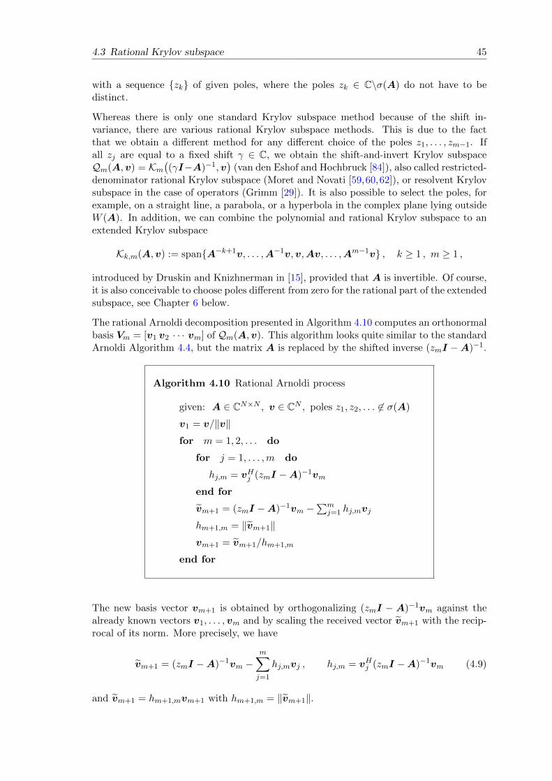
4.3 Rational Krylov subspace 45
with a sequence zk of given poles, where the poles zk ∈ C\σ(A) do not have to bedistinct.
Whereas there is only one standard Krylov subspace method because of the shift in-variance, there are various rational Krylov subspace methods. This is due to the factthat we obtain a different method for any different choice of the poles z1, . . . , zm−1. Ifall zj are equal to a fixed shift γ ∈ C, we obtain the shift-and-invert Krylov subspaceQm(A,v) = Km
((γI−A)−1,v
)(van den Eshof and Hochbruck [84]), also called restricted-
denominator rational Krylov subspace (Moret and Novati [59,60,62]), or resolvent Krylovsubspace in the case of operators (Grimm [29]). It is also possible to select the poles, forexample, on a straight line, a parabola, or a hyperbola in the complex plane lying outsideW (A). In addition, we can combine the polynomial and rational Krylov subspace to anextended Krylov subspace
Kk,m(A,v) := spanA−k+1v, . . . ,A−1v,v,Av, . . . ,Am−1v , k ≥ 1 , m ≥ 1 ,
introduced by Druskin and Knizhnerman in [15], provided that A is invertible. Of course,it is also conceivable to choose poles different from zero for the rational part of the extendedsubspace, see Chapter 6 below.
The rational Arnoldi decomposition presented in Algorithm 4.10 computes an orthonormalbasis Vm = [v1 v2 · · · vm] of Qm(A,v). This algorithm looks quite similar to the standardArnoldi Algorithm 4.4, but the matrix A is replaced by the shifted inverse (zmI −A)−1.
Algorithm 4.10 Rational Arnoldi process
given: A ∈ CN×N , v ∈ CN , poles z1, z2, . . . 6∈ σ(A)
v1 = v/‖v‖for m = 1, 2, . . . do
for j = 1, . . . ,m do
hj,m = vHj (zmI −A)−1vm
end for
vm+1 = (zmI −A)−1vm −∑m
j=1 hj,mvj
hm+1,m = ‖vm+1‖vm+1 = vm+1/hm+1,m
end for
The new basis vector vm+1 is obtained by orthogonalizing (zmI − A)−1vm against thealready known vectors v1, . . . ,vm and by scaling the received vector vm+1 with the recip-rocal of its norm. More precisely, we have
vm+1 = (zmI −A)−1vm −m∑j=1
hj,mvj , hj,m = vHj (zmI −A)−1vm (4.9)
and vm+1 = hm+1,mvm+1 with hm+1,m = ‖vm+1‖.

46 4 Krylov subspace methods
In contrast to Algorithm 4.10, the rational Arnoldi algorithm originally considered byRuhe in [69,70] uses
w = Vmym ,
hj,m = vHj
(I − 1
zmA
)−1
Aw , j = 1, . . . ,m
vm+1 =
(I − 1
zmA
)−1
Aw −m∑j=1
hj,mvj ,
where the vector ym should be chosen such that (I− 1zmA)−1Aw ∈ Qm+1(A,v)\Qm(A,v).
Theoretically, it could happen that the rational Arnoldi process 4.10 yields vm+1 = 0and thus breaks down, although the invariance index µ has not yet been reached. Thisis the case, if the previously computed vector is of the form vm = pm−1(A)qm−1(A)−1vand the new pole zm is a root of the polynomial pm−1 ∈ Pm−1. Such a breakdown mightalso appear in the rational Krylov decomposition by Ruhe, if ym has not been suitablyselected. However, in numerical experiments we never have observed such an “unluckybreakdown”.
To obtain a formula similar to the standard Arnoldi decomposition (4.1), we multiply (4.9)by zmI −A and reorder the terms to obtain
Am+1∑j=1
hj,mvj = zm
m+1∑j=1
hj,mvj − vm .
In matrix notation, this relation can also be written as
AVmHm + hm+1,mAvm+1eTm = Vm(HmDm − I) + zmhm+1,mvm+1e
Tm ,
where Hm = (hi,j)mi,j=1 ∈ Cm×m and Dm = diag(z1, . . . , zm).
For the shift-and-invert Krylov subspace Qm(A,v) = Km((γI −A)−1,v
)with zj = γ for
j = 1, . . . ,m− 1, we have the decomposition
(A− γI)VmHm = −Vm + (γI −A)hm+1,mvm+1eTm (4.10)
or
(γI −A)−1Vm = VmHm + hm+1,mvm+1eTm . (4.11)
This is just the standard Arnoldi decomposition, where A is replaced by (γI − A)−1.Consequently, the rational process with a fixed pole γ only breaks down with hm+1,m = 0,if the invariance index µ is reached, as is the case for the standard Arnoldi algorithm(e.g., Saad [73], Proposition 6.6). This is called a “lucky breakdown”, since then f(A)vbelongs to the computed subspace Qµ(A,v). For the shift-and-invert Krylov subspace, arearrangement of (4.10) yields the compression
HHm := VmHAVm = γI −H−1
m − hm+1,mVmHAvm+1e
TmH
−1m , (4.12)
whereas for the general case, we find
HHm := VmHAVm = (HmDm − I)H−1
m − hm+1,mVmHAvm+1e
TmH
−1m .

4.3 Rational Krylov subspace 47
By analogy with the standard Arnoldi approximation (4.2) above, the rational Arnoldiapproximation reads
f(A)v ≈ Vmf(VmHAVm)Vm
Hv = ‖v‖Vmf( HHm)e1 . (4.13)
A slightly different approximation for symmetric and negative semi-definite matrices andthe function f(z) = ez, based on the shift-and-invert Krylov subspace, is discussed byHochbruck and van den Eshof in [84]. The authors consider the transformed functiongγ(t) = eγ−t
−1such that gγ((γI −A)−1) = eA and therefore suggest the approximation
eAv ≈ ‖v‖Vmgγ(Hm)e1 = ‖v‖VmeγI−H−1m e1 ,
where Hm = VmH(γI−A)−1Vm is the matrix in the rational Arnoldi decomposition (4.11).
This approximation is motivated by the fact that eAv is mainly determined by the eigen-values of A with smallest modulus. If we apply the Lanczos process to the shifted andinverted matrix (γI − A)−1, these important eigenvalues are detected faster. Becauseof relation (4.12), the matrix HHm can be seen as a rank-1 modification of γI − H−1
m .This means that the approximation in [84] does not coincide with the rational Arnoldiapproximation defined in (4.13), but yields a similar approximation.
Reviewing our results, one can note that depending on how we compute an orthonormalbasis Vm of Qm(A,v) = Km(A, qm−1(A)−1v), the matrix Vm ∈ CN×m has a differentform. On the one hand, we might determine Vm by the standard Arnoldi Algorithm 4.4using the matrix A and the vector qm−1(A)−1v and, on the other hand, a computation viathe rational Arnoldi Algorithm 4.10 would be possible. Both procedures lead to a differentbasis of the same subspace. This is why all the following statements will be formulated fora general orthonormal basis of Qm(A,v), which not necessarily coincides with the matrixVm obtained by the rational Arnoldi process.
Definition 4.11 Let Vm be an orthonormal basis of the rational Krylov subspace Qm(A,v)and assume that the denominator qm−1 ∈ Pm−1 has no roots in W (A). For a function fanalytic on W (A), the rational Krylov subspace approximation reads
f(A)v ≈ Vmf(Sm)VmHv , Sm = Vm
HAVm .
As for the standard Krylov subspace approximation, this definition is independent of theparticular choice of the orthonormal basis Vm of Qm(A,v). Applying the rational Arnoldiprocess for the computation of Vm, we have Sm = HHm. Analogously to the Ritz valuesabove, we refer to the eigenvalues of the compression Sm = Vm
HAVm of A to Qm(A,v) asrational Ritz values of A.
Defining Am = PmAPm, where Pm = VmVmH is the orthogonal projection onto the
rational Krylov subspace Qm(A,v), similar to Lemma 4.6, we find again that
Vmf(Sm)VmHv = f(Am)v ,
if the considered function f is, additionally, defined at zero.
The next theorem makes a statement about the exactness of the rational Krylov subspaceapproximation for all rational functions in Pm−1/qm−1. According to Lemma 4.7, thisproperty is already known for the standard Krylov subspace and can directly be transferredto rational Krylov subspace methods (see Beckermann and Reichel [4], p. 21).

48 4 Krylov subspace methods
Lemma 4.12 Let Vm be an orthonormal basis of Qm(A,v) and Sm = VmHAVm. For any
rational function r ∈ Pm−1/qm−1, the rational Krylov subspace approximation is exact,that means
r(A)v = Vmr(Sm)VmHv ,
provided that r(Sm) is defined.
Proof. Let w = qm−1(A)−1v and Vm be a basis of Qm(A,v) = Km(A,w). For anarbitrary polynomial pm−1 ∈ Pm−1, Lemma 4.7 gives
pm−1(A)w = Vmpm−1(Sm)VmHw .
Furthermore, we have
v = qm−1(A)w = Vmqm−1(Sm)VmHw ⇐⇒ qm−1(Sm)−1Vm
Hv = VmHw
and therefore
r(A)v = pm−1(A)qm−1(A)−1v = pm−1(A)w = Vmpm−1(Sm)VmHw
= Vmpm−1(Sm)qm−1(Sm)−1VmHv = Vmr(Sm)Vm
Hv ,
which concludes the proof. o
Lemma 4.12 is now exploited to show the following interpolation result (see, e.g., Guttel[30], Theorem 4.8), which is the analogue to relation (4.7) above in the polynomial case.
Lemma 4.13 Assume that f(Sm) is defined. On the condition that the roots of the de-nominator polynomial qm−1 do not coincide with the eigenvalues of Sm, we have
Vmf(Sm)VmHv = r(A)v , Sm = Vm
HAVm ,
where the rational function r ∈ Pm−1/qm−1 interpolates f at the rational Ritz values ofthe matrix A.
Proof. We define g := qm−1f . By Theorem 2.5, we have g(Sm) = pm−1(Sm) for a poly-nomial pm−1 ∈ Pm−1, where pm−1 interpolates g in the Hermite sense at the eigenvaluesof the matrix Sm, that is, at the rational Ritz values of A. From this, we can concludethat r := pm−1/qm−1 interpolates the function f at σ(Sm) in the Hermite sense. For thisreason, we obtain f(Sm) = pm−1(Sm)/qm−1(Sm) and thus
Vmf(Sm)VmHv = Vm
pm−1(Sm)
qm−1(Sm)VmHv = Vmr(Sm)Vm
Hv = r(A)v
with the help of Lemma 4.12. o
In a similar way, other important properties of the polynomial Krylov subspace processcan be transferred to the rational method. These properties include, for example, theexactness property f(A)v = Vµf(Sµ)V H
µ v, if the invariance index µ is reached.

4.3 Rational Krylov subspace 49
0 5 10 1510−10
10−5
100
n = 10
0 10 20 3010−10
10−5
100
n = 20
0 20 4010−10
10−5
100
n = 30
Figure 4.3: Plot of error versus iteration steps of the standard (red dashed line) and therational (blue solid line) Krylov subspace method for the two-dimensional heat equationand n = 10, 20, 30.
Example 4.14 In order to demonstrate the advantages of the rational over the stan-dard Krylov subspace method, we consider the discretization of the two-dimensional heatequation on Ω = (0, 1)2 with homogeneous Dirichlet boundary conditions for the initialfunction
u(0, x, y) = u0(x, y) = 100 · x2(1− x)2y2(1− y)2
‖x2(1− x)2y2(1− y)2‖L2(Ω).
In Section 3.1.1, we have seen that the finite-difference discretization leads to the systemof ordinary differential equations u′(t) = Au(t), u(0) = u0, with solution u(t) = etAu0.We choose n inner grid points in each space direction and set N = n2. Actually, we shouldwrite Ah instead of A to indicate that the discretization matrix depends on the mesh sizeh = 1
n+1 . This is the case in all our numerical experiments, but we will always omit the
subscript h. In this example, the discretization matrix A ∈ RN×N has the field of values
W (A) =
[− 8
h2sin2
(nπ
2(n+ 1)
),− 8
h2sin2
(π
2(n+ 1)
)]on the negative real line with the limit
W (A)→ (−∞,−2π2] for h→ 0 .
We approximate eτAu0 for τ = 0.05 by the standard and a rational Krylov subspacemethod with denominator polynomial qm−1(z) = (1− z)m−1. For n = 10, 20, 30, the com-parison of the obtained error curves is shown in Figure 4.3. It becomes evident that therational Krylov subspace method achieves a high accuracy in a few iteration steps inde-pendent of the grid spacing h = 1
n+1 , whereas the convergence behavior of the polynomialmethod deteriorates the larger the value n is chosen. This effect can be explained by theerror bound (4.8) that predicts a superlinear convergence only after m ≥
√‖τA‖ Krylov
steps. Since ‖τA‖ is proportional to τh2 , it is not surprising that the convergence is worse,
if we decrease the mesh size h.
In order to prove a grid-independent convergence, we therefore need a uniform error boundthat applies to all matrices with an arbitrary field of values on the negative real line. Withregard to general evolution equations of parabolic or hyperbolic type, we have to look forerror estimates that are uniform for all matrices with an arbitrarily large field of values inthe left complex half-plane. This condition can never be fulfilled by a polynomial Krylovsubspace method, but we will see later in this thesis that rational Krylov subspace methodsare suitable to approximate uniformly matrix functions of such stiff matrices and henceguarantee a grid-independent convergence. m

50 4 Krylov subspace methods
4.4 Near-optimality of the Krylov subspace approximation
The exactness property of the standard and the rational Krylov subspace method inLemma 4.7 and 4.12 can be used to bound the error ‖f(A)v − Vmf(Sm)Vm
Hv‖ of theKrylov subspace approximation by a scalar approximation problem on the field of valuesW (A). For this purpose, we need a helpful theorem of Crouzeix [12].
Lemma 4.15 For an arbitrary matrix A and any polynomial p, we have
‖p(A)‖ ≤ C supz∈W (A)
|p(z)| , C ≤ 11.08 .
Crouzeix conjectures that this bound can be improved to C = 2. By Runge’s Theorem, cf.Corollary 12.1.2 in [28], the function f can be uniformly approximated by a polynomialon W (A), if f is analytic in a neighborhood of W (A). A density argument then makes itpossible to generalize Lemma 4.15 to any function f that is analytic in a neighborhood ofthe field of values: Let Σ be a set with W (A) ⊆ Σ, then
‖f(A)‖ ≤ C supz∈Σ|f(z)| (4.14)
holds true. This estimate is a very powerful tool, which enables us to formulate a well-known result concerning the near-optimality of the polynomial and the rational Krylovsubspace approximation.
Theorem 4.16 Let Sm = VmHAVm be the compression of A onto the standard Krylov
subspace Km(A,v) and let the function f be analytic in a neighborhood of W (A). Thenfor any set Σ ⊇W (A), we have
‖f(A)v − Vmf(Sm)VmHv‖ ≤ 2 C‖v‖ min
p∈Pm−1
supz∈Σ|f(z)− p(z)| .
The same holds true, if Sm = V Hm AVm is the compression of A onto the rational Krylov
subspace Qm(A,v), that is,
‖f(A)v − Vmf(Sm)V Hm v‖ ≤ 2 C‖v‖ min
r∈Pm−1qm−1
supz∈Σ|f(z)− r(z)| .
Proof. Due to Lemma 4.7, we know in the first case that p(A)v = Vmp(Sm)VmHv for
any polynomial p ∈ Pm−1. Since Vm has orthonormal columns by assumption, we have‖Vmx‖ = ‖x‖ for all x ∈ CN . Moreover, VmVm
H is the projection onto Km(A,v), suchthat VmVm
Hv = v and thus ‖VmHv‖ = (vHVmVmHv)1/2 = ‖v‖. This yields
‖f(A)v − Vmf(Sm)VmHv‖ = ‖f(A)v − p(A)v + Vmp(Sm)Vm
Hv − Vmf(Sm)VmHv‖
≤ ‖f(A)− p(A)‖‖v‖+ ‖p(Sm)− f(Sm)‖‖v‖
≤ 2 C‖v‖ supz∈Σ|f(z)− p(z)| ,
where the last inequality is obtained by (4.14) and the fact that W (Sm) ⊆ W (A). Ifwe take the minimum over all polynomials p ∈ Pm−1, the first statement of the theoremis proved. Analogously, using Lemma 4.12, the second estimate for the rational Krylovsubspace approximation can be shown. o

4.4 Near-optimality of the Krylov subspace approximation 51
For normal matrices, the bounds in Theorem 4.16 hold with C = 1 and Σ = σ(A) ∪ σ(Sm):Since in this case A is unitary diagonalizable, that is, A = UDUH with unitary U and adiagonal matrix D, it follows
‖f(A)v − p(A)v‖ ≤ ‖U(f(D)− p(D)
)UH‖‖v‖ ≤ ‖v‖ sup
z∈σ(A)|f(z)− p(z)|
for any polynomial p ∈ Pm−1. Analogously, we derive
‖f(A)v − r(A)v‖ ≤ ‖v‖ supz∈σ(A)
|f(z)− r(z)|
for any rational function r ∈ Pm−1/qm−1. The same applies for ‖f(Am)v− p(Am)v‖ and‖f(Am)v − r(Am)v‖.
Theorem 4.16 has a far-reaching consequence: In order to find an error bound for theKrylov subspace approximation, we may study the scalar best approximation problem
minp∈Pm−1
supz∈Σ|f(z)− p(z)| or min
r∈Pm−1qm−1
supz∈Σ|f(z)− r(z)|
on a set Σ ⊇ W (A). Whereas for the polynomial problem there exists a unique best ap-proximation, the rational best approximation exists, but it might not be unique (e.g., [87]).
The exponential function f(z) = ez, for example, can be approximated by a truncatedTaylor series, Chebyshev or Faber polynomials, see, for instance, [6,41,72,81]. Since poly-nomials are unbounded on unbounded domains, the results achieved with these approachesare only useful, if W (A) is a bounded set of moderate size in the complex plane.
Possible rational approximations are Pade, Chebyshev-Pade or Caratheodory-Fejer ap-proximations and methods which are based on the Faber transform for rational functionsor the application of a quadrature rule to a suitable contour integral, e.g., [4,34,75,83]. Anatural candidate for the latter is the Cauchy integral formula
f(z) =1
2πi
∫Γ
f(ξ)
ξ − zdξ ,
where Γ is a path with parametrization Γ(t) winding around W (A). Applying the trun-cated trapezoidal rule with m − 1 equally spaced nodes wk of distance h, we obtain therational approximation
f(z) ≈ r(z) =h
2πi
m−1∑k=1
f(Γ(wk)
)Γ(wk)− z
Γ′(wk) .
Another way to obtain upper bounds for the standard and the rational Krylov subspaceapproximation relies on a scalar problem of approximating f by an interpolating polyno-mial p or an interpolating rational function r. This approach uses the following formulasgiven in Walsh [87] (Chapter III, equation (4) and Chapter VIII, Theorem 2): Let thefunction f be analytic in a domain Σ ⊂ C and let p ∈ Pm−1 interpolate f at the nodesα1, . . . , αm ∈ Σ. If Γ is a contour in Σ encircling α1, . . . , αm, we have the error represen-tation
f(z)− p(z) =1
2πi
∫Γ
sm,0(z)
sm,0(ξ)
f(ξ)
ξ − zdξ , z ∈ int(Γ) ,

52 4 Krylov subspace methods
where sm,0(z) = (z − α1) · · · (z − αm). Similarly, the error for the approximation of f bya rational function r with interpolation nodes α1, . . . , αm and poles β1, . . . , βm−1 distinctfrom the values αk, k = 1, . . . ,m, is given by
f(z)− r(z) =1
2πi
∫Γ
sm,m−1(z)
sm,m−1(ξ)
f(ξ)
ξ − zdξ , z ∈ int(Γ) , z 6∈ β1, . . . , βm−1
with
sm,m−1(z) =(z − α1) · · · (z − αm)
(z − β1) · · · (z − βm−1).
This leads to the difficult task to select the nodes αk, the poles βk, and the contour Γ insuch a way that
maxz∈Σ |sm,j(z)|minξ∈Γ |sm,j(ξ)|
, j ∈ 0,m− 1 (4.15)
is as small as possible, in order to give a reasonable error estimate. This leads to toolsfrom logarithmic potential theory (see, for instance, [30]). However, it would go beyondthe scope of this thesis to get into further details about this theory here.
In all these cases, it has to be ensured that the roots z1, . . . , zm−1 of the prescribeddenominator polynomial qm−1(z) of the rational Krylov subspace method must coincidewith the poles of the chosen rational approximation r(z). This means, in particular, thatthe poles have to be known in advance.
Moreover, there exist rational Krylov subspace methods that use an automated parameterselection. For functions of Cauchy-Stieltjes type3, the authors in [32] suggest to choose thenext pole zm such that |sm,m−1(zm)| = minξ∈Γ |sm,m−1(ξ)|. This strategy aims to makethe denominator in (4.15) as large as possible.
4.5 Generalization and computation of the Krylov subspaceapproximation
Previously, we only considered the Euclidean inner product. In this section, we generalizethe Krylov subspace approximation to arbitrary inner products (· , ·)M on CN , whereM ∈ CN×N is a fixed positive definite Hermitian matrix. In this case, we have the verysimilar formula
f(A)v ≈ f(Am)v = Vmf(Sm)Vm+v (4.16)
for any function f that is analytic on W (A) and defined at the point zero. Like before,Sm = Vm
+AVm ∈ Cm×m is the compression andAm = PmAPm is the restriction ofA ontothe Krylov subspace. The matrix Pm = VmVm
+ = VmVmHM designates the orthogonal
projection on the Krylov subspace with respect to the inner product (· , ·)M on CN andVm
+ = VmHM is the Moore-Penrose inverse of Vm defined in Definition 4.1 associated to
(· , ·)M . Using the approximation (4.16), the problem of computing f(A)v for a largeN -by-N matrix A is reduced to the evaluation of Vmf(Sm)Vm
+v. In this case, we onlyhave to evaluate a matrix function for the small matrix Sm of size m ×m with m N .This can be done by standard algorithms for dense matrices.
3Functions of Cauchy-Stieltjes type can be written in the form f(z) =∫
Γ(z−x)−1dµ(x) with some measure
µ supported on a closed set Γ ⊂ C.

4.5 Generalization and computation of the Krylov subspace approximation 53
Krylov subspaces can also be defined for operators A on some Hilbert space H. For thispurpose, we replace the matrix A and the vector v by the operator A and a vector v ∈ H.The Krylov subspace approximation to the operator function f(A) times v is definedanalogously by f(Am)v = f(PmAPm)v, where Pm is the orthogonal projector onto theconsidered Krylov subspace Km(A, v) or Qm(A, v).
While it is clear how f(Am)v is computed in the discrete case, we have to think about whatis meant by the notation f(Am)v = f(PmAPm)v in the case of an operator. According toSection 4.1, the projection operator Pm reads Pm = VmV
+m , where Vm is the quasi-matrix
Vm = [v1 · · · vm] with vj ∈ H for j = 1, . . . ,m, that contains an orthonormal basis of theKrylov subspace. The Moore-Penrose inverse V +
m applied to v ∈ H is understood as thevector
V +m v =
(v, v1)(v, v2)
...(v, vm)
∈ Cm ,
containing all inner products of v and the basis functions v1, . . . , vm of the space ontowhich we want to project. We also need the compression V +
mAVm of the operator A ontothe Krylov subspace that is computed to
V +mAVm =
(Av1, v1) · · · (Avm, v1)...
...(Av1, vm) · · · (Avm, vm)
∈ Cm×m ,
which we also designate with Sm in analogy to the discrete case. Then the Krylov subspaceapproximation for operator functions is given by
f(A)v ≈ f(Am)v = Vmf(Sm)V +m v = Vm g =
m∑j=1
gjvj ∈ H ,
where g = (gj)mj=1 = f(Sm)V +
m v ∈ Cm and Sm = V +mAVm ∈ Cm×m. This shows that
even in the case of operators, we only have to compute a matrix function f(Sm) of a smallm×m - matrix, which is then multiplied by the vector V +
m v ∈ Cm.
For our purposes, mainly f(z) = ϕ`(z) is of great interest. In particular, we have seenthat, generally, every time step in the exponential integrator requires the evaluation of thelinear combination
ϕ0(τA)w0 + ϕ1(τA)w1 + . . .+ ϕs(τA)ws
of the matrix ϕ-functions acting on certain vectors wj . The approximation of ϕ`(τA)wj
by a Krylov subspace method leads to expressions of the type Vmϕ`(τSm)Vm+wj .
For the computation of ϕ`(Sm) times a vector v, there exists an elegant way based on anidea of Saad [72]. He used an augmented matrix HSm and calculated the matrix exponentialof HSm to obtain bTϕ1(Sm) for any vector b ∈ Cm. This result was generalized by Sidje [77]to the computation of ϕ`(Sm)v for an arbitrary vector v ∈ Cm with the help of theaugmented matrix
HSm+` =
Sm vI`−1
0 · · · 0
∈ C(m+`)×(m+`) ,
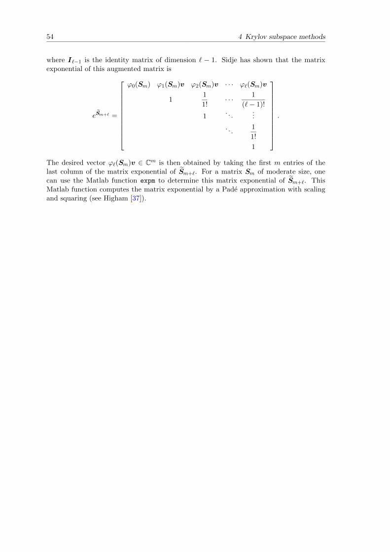
54 4 Krylov subspace methods
where I`−1 is the identity matrix of dimension ` − 1. Sidje has shown that the matrixexponential of this augmented matrix is
e SSm+` =
ϕ0(Sm) ϕ1(Sm)v ϕ2(Sm)v · · · ϕ`(Sm)v
11
1!· · · 1
(`− 1)!
1. . .
...
. . .1
1!
1
.
The desired vector ϕ`(Sm)v ∈ Cm is then obtained by taking the first m entries of thelast column of the matrix exponential of HSm+`. For a matrix Sm of moderate size, onecan use the Matlab function expm to determine this matrix exponential of HSm+`. ThisMatlab function computes the matrix exponential by a Pade approximation with scalingand squaring (see Higham [37]).

Chapter 5
Shift-and-invert Krylov subspaceapproximation
In this chapter, we consider for γ > 0 the approximation of f(A)v in the so-called shift-and-invert Krylov subspace Qm(A,v) with denominator qm−1(z) = (γ − z)m−1, that is
Qm(A,v) = Km((γI −A)−1,v
)= span
v,
1
γ −Av, . . . ,
1
(γ −A)m−1v
(5.1)
for an arbitrary vector v ∈ CN and a large matrix A ∈ CN×N with a field of valuessomewhere in the left complex half-plane, that means
W (A) ⊆ C−0 = z ∈ C : Re(z) ≤ 0 .
For the chosen inner product (· , ·) on CN , the required condition W (A) ⊆ C−0 is equivalentto the relation Re(Av,v) ≤ 0 for all v ∈ CN . We designate by ‖ · ‖ the norm associatedwith the inner product on CN . As matrix norm, we always choose the induced norm thatwe denote with ‖ · ‖, too.
In the context of exponential integrators, we are particularly interested in the special casef(z) = ϕ`(z) and matricesA stemming from a spatial discretization of a partial differentialequation. For fine discretizations, such matrices typically have a widely distributed fieldof values in the left complex half-plane and a huge norm. Exponential integrators havethe favorable property that the temporal convergence results are independent of ‖A‖.Furthermore, they can be regarded as explicit schemes without a severe restriction of thetime step size, even if the norm of the discretization matrix is very large. To preservethese benefits, it is important to approximate the matrix ϕ-functions independent of ‖A‖.We will derive error bounds for the shift-and-invert Krylov subspace method which satisfythis requirement.
In order to do this, we first approximate the matrix function f(A) in the matrix subspace
Rm(A) = span
I,
1
γ −A, . . . ,
1
(γ −A)m−1
. (5.2)
This result can then be used to bound the error for the approximation of f(A)v in therational Krylov subspace Rm(A)v = Qm(A,v). Since it will become apparent that f(A)can be approximated uniformly in Rm(A) for every matrix A with W (A) ⊆ C−0 , this isalso true for the shift-and-invert Krylov subspace approximation to f(A)v. Whenever thenotation Qm(A,v) is used in this chapter, we always mean the shift-and-invert Krylovsubspace defined in (5.1) with denominator qm−1(z) = (γ − z)m−1.
We also discuss possible choices of the free parameter γ > 0, that speed up our convergencerate. Moreover, following the paper [29] by Grimm, we resume the results for abstractevolution equations and the approximation of operator functions f(A)v in a so-calledresolvent Krylov subspace spanned by powers of the resolvent (γI−A)−1 and the vector v.

56 5 Shift-and-invert Krylov subspace approximation
5.1 Transformation to the unit disk
In order to estimate the error for the approximation of f(A) in the rational matrix spaceRm(A) defined in (5.2), we first reduce the problem to a scalar approximation problemon C−0 by using Crouzeix’s inequality (4.14). Afterwards, the problem of approximatingf(z) in the left complex half-plane is transformed to an approximation problem on theunit circle, where well-known results for trigonometric approximation can be applied.
In the following, we denote by D the open unit disk in the complex plane and by D theclosed unit disk with boundary ∂D, that is,
D := z ∈ C : |z| < 1 , D := z ∈ C : |z| ≤ 1 , ∂D := z ∈ C : |z| = 1 .
Similar to Lemma 4.9, the next lemma provides an alternative representation of the matrixspace Rm(A), that will be useful for later purposes.
Lemma 5.1 We have(γ+Aγ−A
)m ∈ Rm+1(A) for m = 0, 1, 2, . . . and γ > 0. Moreover, itholds that
Rm(A) = span
I,
1
γ −A, . . . ,
1
(γ −A)m−1
= span
I,γ +A
γ −A, . . . ,
(γ +A
γ −A
)m−1.
Proof. We exploit the identity γγ−A −
Aγ−A = I to obtain
γ +A
γ −A=
γ
γ −A+
A
γ −A=
2γ
γ −A− I ∈ R2(A) . (5.3)
Since the identity matrix I commutes with any matrix, we can conclude(γ +A
γ −A
)k=
(2γ
γ −A− I
)k=
k∑j=0
(k
j
)(−1)k−j(2γ)j
(1
γ −A
)j∈ Rk+1(A)
by the binomial theorem. This proves the inclusion “⊇ ”. To show the missing inclusion“⊆ ”, we use (5.3) to find
1
γ −A=
1
2γ
(I +
γ +A
γ −A
).
This gives(1
γ −A
)k=
(1
2γ
)k (I +
γ +A
γ −A
)k
=
(1
2γ
)k k∑j=0
(k
j
)(γ +A
γ −A
)j∈ span
I,γ +A
γ −A, . . . ,
(γ +A
γ −A
)k
and our lemma is proved. o
This lemma enables us to turn the best approximation problem
infr∈Pm−1
qm−1
‖f(A)− r(A)‖ = infak
∥∥∥∥∥f(A)−m−1∑k=0
ak1
(γ −A)k
∥∥∥∥∥ ,
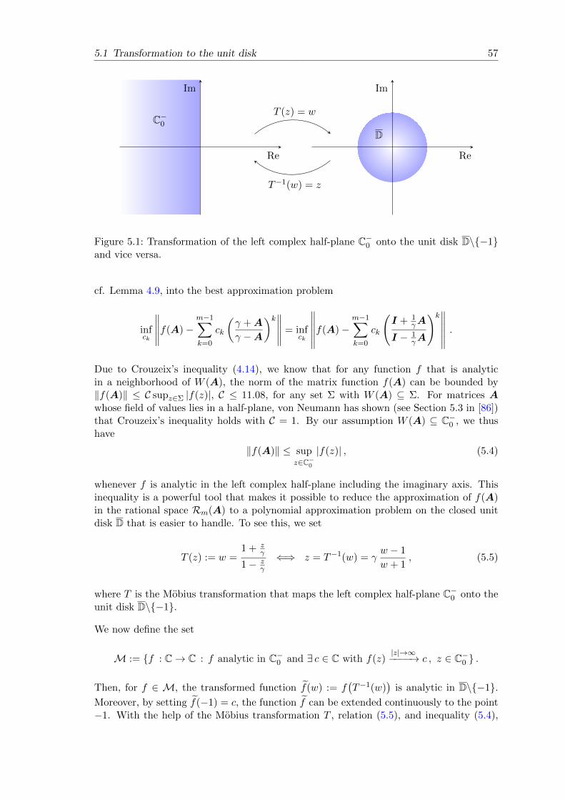
5.1 Transformation to the unit disk 57
C−0
Re
Im
T (z) = w
T−1(w) = z
D
Re
Im
Figure 5.1: Transformation of the left complex half-plane C−0 onto the unit disk D\−1and vice versa.
cf. Lemma 4.9, into the best approximation problem
infck
∥∥∥∥∥f(A)−m−1∑k=0
ck
(γ +A
γ −A
)k∥∥∥∥∥ = infck
∥∥∥∥∥∥f(A)−m−1∑k=0
ck
(I + 1
γA
I − 1γA
)k∥∥∥∥∥∥ .Due to Crouzeix’s inequality (4.14), we know that for any function f that is analyticin a neighborhood of W (A), the norm of the matrix function f(A) can be bounded by‖f(A)‖ ≤ C supz∈Σ |f(z)|, C ≤ 11.08, for any set Σ with W (A) ⊆ Σ. For matrices Awhose field of values lies in a half-plane, von Neumann has shown (see Section 5.3 in [86])that Crouzeix’s inequality holds with C = 1. By our assumption W (A) ⊆ C−0 , we thushave
‖f(A)‖ ≤ supz∈C−0
|f(z)| , (5.4)
whenever f is analytic in the left complex half-plane including the imaginary axis. Thisinequality is a powerful tool that makes it possible to reduce the approximation of f(A)in the rational space Rm(A) to a polynomial approximation problem on the closed unitdisk D that is easier to handle. To see this, we set
T (z) := w =1 + z
γ
1− zγ
⇐⇒ z = T−1(w) = γw − 1
w + 1, (5.5)
where T is the Mobius transformation that maps the left complex half-plane C−0 onto theunit disk D\−1.
We now define the set
M := f : C→ C : f analytic in C−0 and ∃ c ∈ C with f(z)|z|→∞−−−−→ c , z ∈ C−0 .
Then, for f ∈ M, the transformed function f(w) := f(T−1(w)
)is analytic in D\−1.
Moreover, by setting f(−1) = c, the function f can be extended continuously to the point−1. With the help of the Mobius transformation T , relation (5.5), and inequality (5.4),

58 5 Shift-and-invert Krylov subspace approximation
we now obtain the estimate∥∥∥∥∥∥f(A)−m−1∑k=0
ck
(I + 1
γA
I − 1γA
)k∥∥∥∥∥∥ ≤ supz∈C−0
∣∣∣∣∣∣f(z)−m−1∑k=0
ck
(1 + z
γ
1− zγ
)k∣∣∣∣∣∣≤ max
w∈D
∣∣∣∣∣f(γw − 1
w + 1
)−m−1∑k=0
ckwk
∣∣∣∣∣= max
w∈D
∣∣∣∣∣f(w)−m−1∑k=0
ckwk
∣∣∣∣∣ .For the sake of brevity and a clear representation, we additionally introduce at this pointthe short notations f(t) := f
(T−1(eit)
)and T := [0, 2π).
If we assume that f ∈M, the transformed function f is analytic on D and continuous onD and we can conclude with the Maximum Modulus Theorem from complex analysis that
maxw∈D
∣∣∣∣∣f(w)−m−1∑k=0
ckwk
∣∣∣∣∣ = maxw∈∂D
∣∣∣∣∣f(w)−m−1∑k=0
ckwk
∣∣∣∣∣ = maxt∈T
∣∣∣∣∣f(t)−m−1∑k=0
ckeitk
∣∣∣∣∣ .So, we are now concerned with a trigonometric approximation problem for the 2π-periodicfunction f(t) on T. For this purpose, we split f(t) into its real and imaginary partand apply a result of Achyeser [1] to the 2π-periodic real-valued functions Re[f(t)] andIm[f(t)]. His result, formulated in the subsequent theorem, is based on Jackson’s well-known theorem about the error of the best uniform approximation to a real-valued periodicfunction by a trigonometric polynomial. Achyeser’s theorem involves the modulus ofcontinuity ω(g, δ), which we state in the following definition.
Definition 5.2 The modulus of continuity ω(g, δ), δ > 0, of a real-valued continuousfunction g is defined as
ω(g, δ) := sup|s−t|≤δ
|g(s)− g(t)| .
In particular, if g is a 2π-periodic and continuous function, we have
ω(g, δ) = sup0<h≤δ
maxt∈T|g(t+ h)− g(t)| .
Theorem 5.3 (Achyeser [1], Section 4) Let g be a 2π-periodic real-valued function thatis n times continuously differentiable. Then there exists a trigonometric polynomial
Jm,n(g, t) =a0
2+m−1∑k=1
Dk(m,n)(ak cos(kt) + bk sin(kt)
), (5.6)
where ak, bk are the Fourier coefficients of the function g and Dk(m,n) are real constantsthat depend on m and n, such that
maxt∈T|g(t)− Jm,n(g, t)| ≤ C(n)
mnω
(g(n),
1
m
)with a constant C(n) that depends only on n.

5.1 Transformation to the unit disk 59
The proof of this theorem is based on the Jackson integral
Jn(x) =1
2λn
∫Tf(x+ t)
(sin(nt2
)n sin
(t2
))4
dt =1
2λn
∫Tf(x+ t)Kn(t) dt , n ∈ N ,
where 12λnKn(t) is the so-called Jackson kernel and the constant λn is defined by the
relation∫T
12λnKn(t) dt = 1. In [1], Achyeser uses a slightly different representation of the
Jackson integral by de la Vallee Poussin [13] that is given as
Jn(x) =3
2π
∫Rf
(x+
2t
n
)(sin(t)
t
)4
dt , n ∈ N .
The Jackson integrals Jn(x) and Jn(x) are trigonometric polynomials of degree 2n − 2(cf. [54], p. 55) respectively 2n− 1 (cf. [1]). They are applied in approximation theory inorder to bound the best trigonometric approximation of a periodic function. Using theintegral Jn(x), Achyeser has proved the bound in Theorem 5.3 only for the case that mis even. If we make use of the representation Jn(x) instead of Jn(x), it turns out that theresult is also valid for odd values of m.
The expression Jm,n(g, t) in Theorem 5.3 looks quite similar to the (m−1)st partial Fouriersum of the function g that is given by
Sm−1g(t) =a0
2+
m−1∑k=1
ak cos(kt) + bk sin(kt)
with Fourier coefficients
ak =1
π
∫ 2π
0g(t) cos(kt) dt , bk =
1
π
∫ 2π
0g(t) sin(kt) dt ,
except for the fact that the sum in (5.6) contains additional constants Dk(m,n). Theseconstants are specified by the Jackson kernel.
Achyeser’s Theorem 5.3 is only applicable to real-valued and not to complex-valued func-tions. Therefore, we have to subdivide our problem into two real approximation problems:one for the real part and one for the imaginary part. But since we want to examine theexpression infck maxt∈T |f(t)−
∑m−1k=0 cke
itk|, it is not possible to simply approximate the
real and imaginary part of f(t) separately from each other. The trigonometric approxima-tion of the two parts is coupled by the common coefficients ck. Only the special form ofthe Fourier coefficients associated to Re[f(t)] and Im[f(t)] will allow us to consider thesetwo terms independently. More precisely, we exploit the fact that if the Fourier coefficientsof Re[f(t)] are given as aRe
k and bRek , then Im[f(t)] has the Fourier coefficients aIm
k = −bRek
and bImk = aRek . This is the content of the next lemma.
Lemma 5.4 Let the complex function f(w) be analytic in D and continuous on D. Denoteby aRe
k , bRek the Fourier coefficients of the real part Re[f(eit)] = Re[f(t)] and by aIm
k , bImkthe Fourier coefficients of the imaginary part Im[f(eit)] = Im[f(t)]. Then the Fouriercoefficients satisfy
aRek = bImk , bRe
k = −aImk , k ≥ 1 .

60 5 Shift-and-invert Krylov subspace approximation
Proof. For k ≥ 1, the function f(w)wk−1 = f(T−1(w)
)wk−1 is holomorphic in D and
continuous on D. By Cauchy’s integral theorem, the integral of f(w)wk−1 over the closedcurve ∂D is zero. This yields
0 =
∫∂Df(w)wk−1 dw =
∫ 2π
0f(eit)ieikt dt
=
∫ 2π
0
(Re[f(t)] + i Im[f(t)]
)(i cos(kt)− sin(kt)
)dt
= −∫ 2π
0Re[f(t)] sin(kt) + Im[f(t)] cos(kt) dt
+ i
∫ 2π
0Re[f(t)] cos(kt)− Im[f(t)] sin(kt) dt
= −π (bRek + aIm
k ) + i π (aRek − bImk ) .
This implies aRek = bImk and bRe
k = −aImk , which proves the assertion. o
With regard to Theorem 5.3, the idea is now to choose the coefficients ck in the approxi-mation problem maxt∈T |f(t)−
∑m−1k=0 cke
itk| as
c∗0 = a0 − ib0 , c∗k = Dk(m,n)(ak − ibk) ,
a0 =aRe
0
2, b0 = −a
Im0
2, ak = aRe
k , bk = bRek for 1 ≤ k ≤ m− 1 ,
(5.7)
where Dk(m,n) are the coefficients of the trigonometric polynomial Jm,n in Theorem 5.3.
This enables us to separate the approximation problem for f(t), t ∈ T, into two indepen-dent subproblems for the real and imaginary part in the following way:
infck
maxt∈T
∣∣∣f(t)−m−1∑k=0
ckeitk∣∣∣ ≤ max
t∈T
∣∣∣∣∣f(t)−m−1∑k=0
c∗keitk
∣∣∣∣∣≤max
t∈T
∣∣∣f(t)− (a0 − ib0)−m−1∑k=1
Dk(m,n)(ak − ibk)(
cos(kt) + i sin(kt))∣∣∣
= maxt∈T
∣∣∣Re[f(t)]− a0 −m−1∑k=1
Dk(m,n)(ak cos(kt) + bk sin(kt)
)+ i Im[f(t)] + ib0 − i
m−1∑k=1
Dk(m,n)(− bk cos(kt) + ak sin(kt)
)∣∣∣≤max
t∈T
∣∣∣Re[f(t)]− aRe0
2−m−1∑k=1
Dk(m,n)(aRek cos(kt) + bRe
k sin(kt))∣∣∣ (5.8)
+ maxt∈T
∣∣∣Im[f(t)]− aIm0
2−m−1∑k=1
Dk(m,n)(aImk cos(kt) + bImk sin(kt)
)∣∣∣ , (5.9)
where we have used Lemma 5.4 and (5.7) for the last inequality. The application of

5.2 Error bounds for f ∈M 61
Theorem 5.3 to the terms (5.8) and (5.9) finally gives
infck
maxt∈T
∣∣∣f(t)−m−1∑k=0
ckeitk∣∣∣ ≤ C(n)
mn
[ω
(Re[ f ](n),
1
m
)+ ω
(Im[ f ](n),
1
m
)], (5.10)
if f is n times continuously differentiable. The moduli for the real and imaginary part in(5.10) can be combined to one modulus of continuity for f (n) on T.
Lemma 5.5 The two moduli of continuity in (5.10) fulfill the inequality
ω
(Re[ f ](n),
1
m
)+ ω
(Im[ f ](n),
1
m
)≤ 2ω
(f (n),
1
m
),
where the last modulus ω(f (n), 1m) has to be understood as generalization of Definition 5.2
to complex-valued functions g : R→ C.
Proof. Because of∣∣∣Re[f(t+ h)](n) − Re[f(t)](n)∣∣∣ ≤ ∣∣∣f (n)(t+ h)− f (n)(t)
∣∣∣ ,∣∣∣Im[f(t+ h)](n) − Im[f(t)](n)∣∣∣ ≤ ∣∣∣f (n)(t+ h)− f (n)(t)
∣∣∣for all t ∈ T and 0 < h ≤ 1
m , we conclude that
sup0<h≤ 1
m
maxt∈T
∣∣∣Re[f(t+ h)](n) − Re[f(t)](n)∣∣∣︸ ︷︷ ︸
= ω(Re[ f ](n), 1
m
)≤ sup
0<h≤ 1m
maxt∈T
∣∣∣f (n)(t+ h)− f (n)(t)∣∣∣︸ ︷︷ ︸
= ω(f (n), 1
m
),
sup0<h≤ 1
m
maxt∈T
∣∣∣Im[f(t+ h)](n) − Im[f(t)](n)∣∣∣︸ ︷︷ ︸
= ω(Im[ f ](n), 1
m
)≤ sup
0<h≤ 1m
maxt∈T
∣∣∣f (n)(t+ h)− f (n)(t)∣∣∣︸ ︷︷ ︸
= ω(f (n), 1
m
).
This yields the desired inequality. o
For practical computations, it is in general easier to estimate the moduli for the real andimaginary part separately instead of investigating the modulus of continuity for the wholefunction f (n) on T.
How the inequality (5.10) for the best trigonometric approximation of f(t) can be used tobound the Krylov subspace approximation error for functions f ∈M will be discussed inthe next section. Furthermore, we will estimate the two moduli of continuity of the realand imaginary part for the special case f(t) = ϕ`(t), ` ≥ 1.
5.2 Error bounds for f ∈ M
Let W (A) ⊆ C−0 and f ∈ M. We summarize the ideas of the previous section andconclude that the best approximation of f(A) in the rational matrix subspace Rm(A) can

62 5 Shift-and-invert Krylov subspace approximation
be bounded by
infr∈Pm−1
qm−1
‖f(A)− r(A)‖ ≤ infck
supz∈C−0
∣∣∣∣∣∣f(z)−m−1∑k=0
ck
(1 + z
γ
1− zγ
)k∣∣∣∣∣∣≤ inf
ckmaxt∈T
∣∣∣∣∣f(t)−m−1∑k=0
ckeitk
∣∣∣∣∣ ≤ maxt∈T
∣∣∣∣∣f(t)−m−1∑k=0
c∗keitk
∣∣∣∣∣ ≤ C(n)
mnω
(f (n),
1
m
),
(5.11)
whenever f(t) ∈ Cn(T). Hereby, the coefficients c∗k are chosen as suggested in (5.7). Recall
that f(t) is defined as f(T−1(eit)
), where T designates the Mobius transformation which
maps the left complex half-plane onto the unit disk. The estimate (5.11) is, in particular,valid for the special rational function
r∗(z) =m−1∑k=0
c∗k
(1 + z
γ
1− zγ
)k∈ Pm−1
qm−1. (5.12)
With these considerations we now derive an upper bound for the error ‖f(A)v−f(Am)v‖of the shift-and-invert Krylov subspace approximation, where Am is given by PmAPmand Pm represents the orthogonal projection onto Qm(A,v) = Km
((γI −A)−1,v
). But
first of all, we must guarantee that W (Am) ⊆ C−0 , such that the projected matrix Am
actually fits in our framework.
Lemma 5.6 If W (A) ⊆ C−0 , the restriction Am = PmAPm of the matrix A ∈ CN×N tothe subspace Qm(A,v) satisfies W (Am) ⊆ C−0 as well.
Proof. The relation W (Am) ⊆ C−0 is equivalent to Re(Amx,x) ≤ 0 for all x ∈ CN .Setting y = Pmx and using the fact that Pm is self-adjoint, cf. Definition 4.1, it follows
Re(Amx,x) = Re(PmAPmx,x) = Re(APmx,Pmx) = Re(Ay,y) ≤ 0 ,
since W (A) ⊆ C−0 by assumption. o
Theorem 5.7 Let A be a matrix with W (A) ⊆ C−0 and suppose f ∈ M. Moreover, for
f(t) = f(T−1(eit)
), we assume that the nth derivative f (n) exists and is continuous on
T. Then the error of the approximation f(Am)v to f(A)v in the shift-and-invert Krylovsubspace Qm(A,v) is bounded by
‖f(A)v − f(Am)v‖ ≤ 2C(n)
mnω
(f (n),
1
m
)‖v‖ ,
where Am = PmAPm and Pm is the orthogonal projection onto Qm(A,v).
Proof. Because of Lemma 5.6 and Lemma 4.12, we know that W (Am) ⊆ C−0 and that
r(A)v = r(Am)v for every r ∈ Pm−1
qm−1with qm−1(z) = (γ − z)m−1 .
We now consider the special rational function r∗ defined in (5.12). Then r∗(A)v belongsto Qm(A,v) and we have r∗(A)v = r∗(Am)v. Since r∗ is determined solely by f and not

5.3 Error bounds for the ϕ-functions 63
by the matrices A or Am, the error bound (5.11) can be applied to ‖f(A) − r∗(A)‖ aswell as to ‖f(Am) − r∗(Am)‖. Using the triangle inequality and (5.11), we are now ableto conclude that
‖f(A)v − f(Am)v‖ ≤ ‖f(A)− r∗(A)‖ ‖v‖+ ‖f(Am)− r∗(Am)‖ ‖v‖
≤ 2C(n)
mnω
(f (n),
1
m
)‖v‖
holds true. o
In a nutshell, this theorem says that the convergence rate of the shift-and-invert Krylovsubspace approximation for f(A)v, f ∈M, depends only on the smoothness properties ofthe transformed function f
(T−1(w)
)on the boundary of the unit circle. The obtained error
bound is completely independent of ‖A‖. Consequently, we have a uniform convergencefor all matrices A with a field of values somewhere in the left complex half-plane.
5.3 Error bounds for the ϕ-functions
The findings of Section 5.2 raise the question what is to be expected for f = ϕ`. For ` ≥ 1,the modulus |ϕ`(z)| tends to zero for all |z| → ∞ with Re(z) ≤ 0, so that ϕ` ∈ M withc = 0. In contrast, we have ϕ0 6∈ M, since |ez| → 0 for Re(z)→ −∞, whereas |ez| = 1 onthe imaginary axis. Thus, Theorem 5.7 can only be used for the ϕ`-functions with ` ≥ 1.According to the previous considerations, we have to analyze the real and imaginary partof ϕ`(t) = ϕ`
(T−1(eit)
)with respect to their differentiability. The next lemma will be
helpful for this purpose.
Lemma 5.8 Both functions x sin(
1x
)and x cos
(1x
), x ∈ R, are 1
2 -Holder continuous onany bounded domain.
Proof. We show the assertion only for the first function x sin(
1x
), since the proof for the
second function x cos(
1x
)can be conducted analogously. We start with∣∣∣∣y sin
(1
y
)− x sin
(1
x
)∣∣∣∣2 =
∣∣∣∣y2 sin2
(1
y
)− 2xy sin
(1
y
)sin
(1
x
)+ x2 sin2
(1
x
)∣∣∣∣ .Due to 2xy = x2 + y2 − (y − x)2 and
∣∣ sin ( 1x
)∣∣ ≤ 1, we get with the triangle inequality∣∣∣∣y sin
(1
y
)− x sin
(1
x
)∣∣∣∣2 ≤ 2
∣∣∣∣y2 sin
(1
y
)− x2 sin
(1
x
)∣∣∣∣+ |y − x|2 .
On a bounded domain, the function x2 sin(
1x
)is Lipschitz continuous, because its deriva-
tive is bounded. It thus follows∣∣∣∣y sin
(1
y
)− x sin
(1
x
)∣∣∣∣ ≤ C |y − x| 12by taking the square root. o

64 5 Shift-and-invert Krylov subspace approximation
π0
2
4
6
8
·10−3
Figure 5.2: Plot of Re[ϕ`(t)] for t ∈ [3, 3.28], ` = 2, and γ = 1.
Theorem 5.9 Let A satisfy W (A) ⊆ C−0 and let Pm be the orthogonal projection ontothe shift-and-invert Krylov subspace Qm(A,v). For the restriction Am = PmAPm of Ato Qm(A,v), we have the error bound
‖ϕ`(A)v − ϕ`(Am)v‖ ≤ C(`, γ)
m`2
‖v‖ , ` ≥ 1 .
Proof. Due to Theorem 5.7, our task is to study the modulus of continuity ω(ϕ(n)` , 1
m).This is equivalent to examine separately the real and imaginary part of ϕ`(t) with respectto its smoothness. Here, we restrict ourselves to the analysis of Re[ϕ`(t)]. The imaginarypart can be estimated analogously. Before we start our investigation, it is worthwhile tomention that
eit − 1
eit + 1= i tan
(t
2
),
so that ϕ`(t) = ϕ`(iγ tan
(t2
)). As composition of infinitely many times differentiable
functions on T\π, T = [0, 2π), the function Re[ϕ`(t)] = Re[ϕ`(iγ tan
(t2
))]is also
infinitely often differentiable for t 6= π. For this reason, we analyze Re[ϕ`(t)] on theinterval Tπ := (π − σ, π + σ) for 0 < σ < π, cf. Figure 5.2. Hereby, it is necessary todistinguish whether the index ` of the ϕ`-function is odd or even. In the following, we willanalyze these two cases one after another.
(i) ` even: Using the representation (3.13) for ϕ`(iγ tan
(t2
)), we find
Re[ϕ`(t)] = (−1)`2
cos(γ tan
(t2
))(γ tan
(t2
))` −`2−1∑k=0
(−1)kγ2k−`
(2k)!tan2k−`
(t
2
) .There is no need to worry about the second term, containing the sum over k, sincetan2k−` ( t
2
)is infinitely often differentiable on Tπ for all k ∈ 0, . . . , `2 − 1. Differ-

5.3 Error bounds for the ϕ-functions 65
entiating the first term with respect to t,
d
dt
cos(γ tan
(t2
))(γ tan
(t2
))` = −1
2
[`γ
cos(γ tan
(t2
))(γ tan
(t2
))`+1+ γ
sin(γ tan
(t2
))(γ tan
(t2
))`+`
γ
cos(γ tan
(t2
))(γ tan
(t2
))`−1+
1
γ
sin(γ tan
(t2
))(γ tan
(t2
))`−2
],
we see that we obtain a linear combination of similar expressions, where the numera-tor is partly replaced by sin
(γ tan
(t2
))and where the exponent of the denominator
has changed by +1, 0, −1 or −2. The different terms are continuously differen-tiable as long as the exponent in the denominator is greater than 2. The functionssin(γ tan
(t2
))/ tan2
(t2
)and cos
(γ tan
(t2
))/ tan2
(t2
)have no continuous derivative,
but their derivatives are bounded on Tπ. This shows that Re[ϕ`(t)] ∈ C`2−1(Tπ) and
ω
(Re[ ϕ` ](
`2−1),
1
m
)≤ C(`, γ)
m,
using the mean value theorem with |Re[ϕ`(ξ)]( `
2)| ≤ C(`, γ) for all ξ ∈ Tπ.
(ii) ` odd: Since now
Re[ϕ`(t)] = (−1)`−1
2
sin(γ tan
(t2
))(γ tan
(t2
))` +
`−12−1∑
k=0
(−1)k+1 γ2k−`+1
(2k + 1)!tan2k−`+1
(t
2
) ,the same considerations as in (i) apply with the exception that the first termsin(γ tan
(t2
))/ tan`
(t2
)can only be differentiated continuously b `2c times for t ∈ Tπ,
until we get expressions of the form
g1(t) :=sin(γ tan
(t2
))γ tan
(t2
) or g2(t) :=cos(γ tan
(t2
))γ tan
(t2
) .
The application of Lemma 5.8 with x = 1/(γ tan
(t2
))and y = 1/
(γ tan
( t+1/m2
))gives for j ∈ 1, 2 the estimate
∣∣∣∣gj (t+1
m
)− gj(t)
∣∣∣∣ ≤ C∣∣∣∣∣∣ 1
γ tan(t+1/m
2
) − 1
γ tan(t2
)∣∣∣∣∣∣
12
≤ C(γ)√m
, t ∈ Tπ ,
where the second inequality follows by the mean value theorem. This yields
ω
(Re[ ϕ` ]b
`2c,
1
m
)≤ C(`, γ)√
m.
Furthermore, note that m−b`/2cm−1/2 = m−`/2.
Together with Theorem 5.7 and a similar estimate for Im[ϕ`(t)], the statement of thetheorem is proved. o
For the best approximation of the matrix function ϕ`(A) in the rational matrix spaceRm(A), the proof of Theorem 5.9 shows, in particular, that
infr∈Pm−1
qm−1
‖ϕ`(A)− r(A)‖ ≤ ‖ϕ`(A)− r∗(A)‖ ≤ C(`, γ)
m`2
, (5.13)

66 5 Shift-and-invert Krylov subspace approximation
where r∗ is the rational function r∗(z) =∑m−1
k=0 c∗k
(1+z/γ1−z/γ
)kin (5.12) with coefficients c∗k
defined by (5.7).
Remark 5.10 When applying numerical methods for the time integration of evolutionequations, one is interested in the approximation of ϕ`(τA)v, where τ > 0 denotes thestep size in time. Since
Re((τA)x,x
)= τ Re(Ax,x) ≤ 0 for all x ∈ CN ,
we have W (τA) ⊆ C−0 in the case that W (A) ⊆ C−0 . As a result, replacing A by τA leadsto exactly the same scalar approximation problem on the unit disk independent of thestep size τ . This has the far-reaching consequence that all of the above theorems remainvalid with the same constants for τA instead of A, that is,
‖ϕ`(τA)v − ϕ`(τAm)v‖ ≤ C(`, γ)
m`2
‖v‖ .
5.4 Choice of the shift γ
So far, the shift γ > 0 has been regarded as a free parameter of the rational matrixsubspace Rm(A) and the shift-and-invert Krylov subspace Qm(A,v). This section aimsto discuss a strategy for a best possible choice of γ. To this end, we will choose γ dependingon the dimension m of the approximation space. In order to obtain suitable conditions forγ, which raise the asymptotic convergence rate, we need another modulus of smoothness,the rth modulus of smoothness ωr(g, δ). In contrast to the previous sections, where weused ω(g(n), δ) for g ∈ Cn(T), this modulus is given by the following definition (see [14]).
Definition 5.11 For δ > 0, the rth modulus of smoothness ωr(g, δ) of a continuous func-tion g is defined as
ωr(g, δ) := sup0<h≤δ
maxt∈T|∆r
h(g, t)| , ∆rh(g, t) =
r∑k=0
(r
k
)(−1)r−kg(t+ kh) , (5.14)
where ∆rh(g, t) is an rth order difference.
The first modulus of continuity ω1(g, δ) coincides with the modulus of continuity ω(g, δ) inDefinition 5.2. Compared to ω(g, δ), which only measures the continuity properties of thefunction g, the modulus ωr(g, δ) is useful for measuring higher smoothness. Furthermore,we have the relations
ωr(g, δ) ≤ δr maxt∈T|g(r)(t)| and ωr+k(g, δ) ≤ δrωk(g(r), δ) , (5.15)
see [14], p. 46.
In order to measure the quality of approximation for a 2π-periodic real-valued function gby its mth partial Fourier sum Smg(t), we make use of the Jackson-Stechkin inequalityfor the best approximation of g by a trigonometric polynomial P ∈ Tm (see, e.g., [14],Chapter 7, Theorem 2.3). The Jackson-Stechkin inequality reads
infP∈Tm
maxt∈T|g(t)− P (t)| ≤ C(r)ωr
(g,
1
m
), (5.16)
where Tm denotes the set of trigonometric polynomials of degree m. With the help of thisinequality, we can formulate the following lemma.

5.4 Choice of the shift γ 67
Lemma 5.12 The approximation of a real 2π-periodic and continuous function g by itsmth partial Fourier sum Smg is bounded by
|g(t)− Smg(t)| ≤ C(r) ln(m)ωr
(g,
1
m
). (5.17)
Proof. A relation between the approximation by the mth partial Fourier sum and thebest trigonometric approximation can be found as Proposition 1.5.2 in Pinsky [66]. Thisproposition states
|g(t)− Smg(t)| ≤(5 + ln(m)
)infP∈Tm
maxt∈T|g(t)− P (t)| .
Due to the Jackson-Stechkin inequality (5.16), we obtain the desired result. o
The same ideas as in Section 5.1 for the estimate of infck maxt∈T |f(t) −∑m−1
k=0 ckeitk| on
page 60, but this time with Dk(m,n) = 1, lead for f ∈M to the bound
‖f(A)v − f(Am)v‖ ≤ C(r) ln(m)
[ωr
(Re[ f ],
1
m
)+ ωr
(Im[ f ],
1
m
)]‖v‖ . (5.18)
Since we approximate the real and imaginary part of the function f(t) by a trigonometricpolynomial of degree less than or equal to m − 1, it should read m − 1 instead of meverywhere in inequality (5.18). It is nevertheless possible to write m, if we slightlychange the generic constant C(r).
In the case that f is n - times continuously differentiable, we immediately get from (5.15)for r = n, k = 1 and Lemma 5.5 that
‖f(A)v − f(Am)v‖ ≤ C(n)
mnln(m)ω
(f (n),
1
m
)‖v‖ .
Compared to Theorem 5.7, we have an additional factor ln(m). This is caused by settingthe constantsDk(m,n) in the trigonometric approximation equal to one and by consideringthe approximation of Re[f(t)] and Im[f(t)] by its (m − 1)st partial Fourier sum, whichis only the best trigonometric approximation in the L2-norm, but not in the maximumnorm. However, we do not have to worry about this extra factor, since ln(m) grows slowerthan any positive power mβ with β > 0.
We now aim to find an optimal shift γ for the case f = ϕ`, ` ≥ 1, in (5.18). Of course, theestimate of ωr(g, δ) requires more effort than the estimate of ω(g(n), δ), since differences∆rh(g, t) of order r are involved. These differences have to be bounded in a suitable manner
and necessitate several case distinctions. Thus, one may wonder why we should now workwith this apparently more complicated modulus of smoothness ωr(g, δ). The reason forthis is the following: If we use the Jackson-Stechkin bound (5.16), we can conclude how theconstants occurring in the estimates of the two moduli ωr(Re[ ϕ` ], 1
m) and ωr(Im[ ϕ` ], 1m)
depend on the parameters γ and r. From this, it is possible to deduce an appropriateparameter γ. In contrast, by analyzing the constants C(`, γ) in the error estimates ofthe previous section, where the modulus ω(g(n), δ) for a function g ∈ Cn(T) was used, wecould not gain any insight into a suitable choice of γ.
For the shift γ, we choose the ansatz γ(m) := mα with α ∈ R. This choice enables us toderive a condition for the parameter α, depending on ` and r, that raises our asymptotic

68 5 Shift-and-invert Krylov subspace approximation
` i j
` even`2
`2 , . . . , `
r 1, . . . , `
`2
`2
` odd b `2c+ 1 b `2c, . . . , `
r 1, . . . , `
Table 5.1: Possible values of i and j in (5.19).
convergence rate of order O(m−`/2). The key advantage of the modulus ωr(g, δ) used hereis that the parameter r is not bounded by the smoothness of g ∈ Cn(T) and can thus bechosen greater than n.
The estimates of the two moduli ωr(Re[ ϕ` ], δ) and ωr(Im[ ϕ` ], δ) are not very difficult,since they partially rely on the ideas of the previous section. However, they are quitetedious and require a case distinction whether r, ` and b`/2c are even or odd. This is whywe do not present here a detailed derivation of the results stated below.
The main ideas are as follows: As in the proof of Theorem 5.9, one has to treat separatelythe two cases t ∈ Tπ = (π−σ, π+σ), 0 < σ < π, and t ∈ T\π. In the first case, the samerepresentation of Re[ϕ`(t)] and Im[ϕ`(t)] via formula (3.13) can be used. The occurringrth order differences are estimated by a suitable Taylor expansion. The calculation revealsthat, thereby, the condition r > `
2 +1 has to be fulfilled. For t ∈ T\π on the other hand,we represent ϕ`(t) by formula (3.12), use the bound
maxt∈[a,b]
|∆rhg(t)| ≤ hr max
t∈[a,b]|g(r)(t)| for g ∈ Cr([a, b]) , a, b ∈ R ,
and Faa die Bruno’s formula, a generalization of the chain rule to higher derivatives.Altogether, the analysis shows that terms of the form
C(r)δi
γ jand C(r)δrγk , k ∈ 1, . . . , r (5.19)
appear with a generic constant C(r). Possible values of i and j are summarized in Ta-ble 5.1. The decisive prefactors, being most restrictive, are δ`/2γ−`/2 and δrγr. Theylead with δ = 1
m and γ = mα to convergence rates of order m−`/2−α`/2 and m−r+αr. Bybalancing these two expressions, we find the condition
− `2− α`
2= −r + αr or α =
r − `2
r + `2
.
This choice of α leads to the improved convergence rate
O(m−
`2
(1+α)),

5.5 The case of operators 69
which tends to O(m−`) for r → ∞. If we increase r, the rate of convergence becomesfaster and faster. But the analysis shows that the occurring constants grow in the worstcase like
(0.792r/ ln(r+ 1)
)r. This results from an estimate using Faa di Bruno’s formula
in combinatorial form and the bound in [5] on Bell numbers. By counting partitions, thesenumbers indicate how many terms in Faa die Bruno’s formula appear. As a result, theparameter r should not be chosen too large, in order to obtain a reasonable error bound.
For example, if we consider the ϕ1-function, we have an improved rate of order O(m−6/7)for the choice r = 3 compared to O(m−`/2) = O(m−1/2). How the choice of γ affects theapproximation behavior is illustrated by the following simple numerical experiment.
Example 5.13 We consider the approxima-tion of ϕ4(A)v in Qm(A,v) for a matrix A ∈C1 000×1 000 with W (A) ⊆ [−100 i, 100 i] anda random vector v of norm 1, which is gen-erated by the Matlab function randn. Theshift γ is chosen as one (black solid line) and,according to the discussion above, as γ = mα
with α = r−2r+2 for r = 6, 12, 24 and m = 20.
In Figure 5.3, the approximation error is plot-ted against the number of iteration steps. Asexpected, we have a better convergence forlarger r. The apprehension that overly larger have a negative effect cannot be observedhere. Hence, the worst case estimate for C(r)above seems to be too pessimistic. m
0 5 10 15 2010−6
10−5
10−4
10−3
10−2
10−1
γ = 1
γ = 201/2
γ = 205/7
γ = 2011/13
Figure 5.3: Error ‖ϕ4(A)v − ϕ4(Am)v‖versus m.
Remark 5.14 Probably, a result similar to Achyeser’s Theorem 5.3 holds true for therth modulus of smoothness which could not be found in standard literature. In this case,estimate (5.18) above would hold true without the factor ln(m).
5.5 The case of operators
The approximation of operator functions f(A)v, especially of ϕ`(A)v, in the resolventspace Qm(A, v) is analyzed in Grimm [29], where A is assumed to be a linear operator ona Hilbert space H satisfying Range(λI−A) = H for some λ with Re(λ) > 0 and the dissi-pativity property Re(Ax, x) ≤ 0 for every x ∈ D(A). The notation Qm(A, v) means thatthe matrix A ∈ CN×N and the vector v ∈ CN in the rational Krylov subspace Qm(A,v)are replaced by the operator A and v ∈ H. Using the Lumer-Phillips Theorem 3.7, we canconclude that A generates a strongly continuous contraction semigroup with ‖eτA‖ ≤ 1for all τ ≥ 0, where ‖ · ‖ designates the norm induced by the inner product on H.
We denote by f(0) : R → C the restriction of a function f : C → C to Re(z) = 0, thatis, f(0)(ζ) = f(iζ) for ζ ∈ R. Moreover, we assume that f is holomorphic and bounded
on C−0 and that f(0) ∈ C(R), Ff(0) ∈ L1(R) and supp(Ff(0)) ⊆ [0,∞), where Ff(0) is theFourier transform of f(0), given as
Ff(0)(s) =1
2π
∫ ∞−∞
e−ixsf(0)(x) dx .

70 5 Shift-and-invert Krylov subspace approximation
For a function f , fulfilling the above assumptions, we use the functional calculus (cf. [18])
f(A) :=
∫ ∞0
esAFf(0)(s) ds ,
which defines a bounded linear operator f(A) with ‖f(A)‖ ≤ ‖Ff(0)‖L1(R). One can showthat the ϕ`-functions, ` ≥ 1, satisfy the required assumptions and that ϕ`(A), defined viathe functional calculus, coincides with the former definition
ϕ`(A) =
∫ 1
0e(1−s)A s`−1
(`− 1)!ds ,
see (3.12). It is shown in [29] that the best approximation of the operator function f(A)in the resolvent subspace
Rm(A) = span(γI −A)−1, . . . , (γI −A)−m , γ > 0
has the bound
infR∈Rm(A)
‖f(A)−R‖ ≤ C ωrφ(f ,
1√m− 1
), f(s) = esFf(0)
(s
γ
),
where r < m − 1 and C is a constant independent of f . The quality of approximationis measured with the so-called weighted φ-modulus of smoothness ωrφ(g, δ) introduced by
De Bonis, Mastroianni and Viggiano in [7] to characterize the K-functional1 of a functiong by its structural properties. The main part of this modulus is defined by
Ωrφ(g, δ) := sup
0<h≤δ‖w∆r
hφ(g, ·)‖L1[4r2h2, 1h2 ]
with the rth symmetric difference
∆rhφ(g, t) =
r∑j=0
(−1)j(r
j
)g
(t+
hφ(t)
2(r − 2j)
),
where 0 < δ ≤ 1, φ(t) =√t and w(t) = e−t for t > 0. For the complete modulus, we now
compose ωrφ(g, δ) as
ωrφ(g, δ) := Ωrφ(g, δ) + inf
p∈Pr−1
‖w(g − p)‖L1(0,4r2δ2) + infq∈Pr−1
‖w(g − q)‖L1( 1δ2,∞) .
A detailed analysis of ωrφ(ϕ`,
1√m−1
)for ϕ`(s) = esFϕ`,(0)
(sγ
)and r = ` shows that
infR∈Rm(A)
‖ϕ`(A)−R‖ ≤ C(`, γ)
m`2
. (5.20)
Like above, we define by Pm the orthogonal projection onto the resolvent Krylov subspaceQm(A, v) and set Am = PmAPm. Then the resolvent Krylov subspace approximation hasthe error bound
‖ϕ`(A)v − ϕ`(Am)v‖ ≤ C(`, γ)
m`2
‖v‖ .
1The general K-functional is given by Kr,φ(f, δr)w,p = infg(r−1)∈ACloc‖w(f−g)‖Lp +δr‖wφrg(r)‖Lp , where
0 < δ ≤ 1, 1 ≤ p ≤ ∞, w is a Laguerre weight of the form w(t) = tαe−t and ACloc is the set of locallyabsolutely continuous functions.

5.6 Numerical experiments 71
The bounds here look quite similar to our bounds in Section 5.3 for the matrix case, exceptfor the fact that the constants C(`, γ) are different. But the modulus of continuity fromDefinition 5.2, used in the new derivation of this bound in Section 5.3, is more commonand much easier to calculate than the weighted φ-modulus of smoothness in this section.
In [29], the shift γ has been regarded as a fixed constant. To improve the convergencerate in [29], we can proceed analogously to Section 5.4 to find an optimal γ. For thispurpose, we examine by a tedious calculation how the terms occurring in the estimate ofωrφ(ϕ`,
1√m−1
)depend on γ > 0. Looking for the most restrictive terms and setting again
γ = mα, α ∈ R, we get a condition that the parameter α should fulfill, namely α = r−`r+`
for ` < r < m− 1. With this choice, we achieve an upgraded convergence rate of order
O(m−
`2
(1+α)), α =
r − `r + `
.
A sketch of the proof can be found in [25]. It should be noted that we do not end up withthe same optimal value for γ and the same improved rate as in Section 5.4. But this is notsurprising, since we used different moduli of smoothness. Again, we should keep in mindthat the predicted convergence is indeed faster for larger values of r, but at the cost of aconstant C(`, γ) in (5.20) that grows like Kr for a fixed constant K > 0.
5.6 Numerical experiments
In our first experiment, we consider a simple test example that validates the theoreticalbounds and that illustrates the faster convergence for ϕ`-functions of larger index ` . Bythe example of a one-dimensional wave equation, the influence of the choice of the shiftγ on the convergence rate is demonstrated in Section 5.6.2. Finally, we compare theshift-and-invert Krylov subspace method with the implicit Euler and the Crank-Nicolsonscheme for a finite-element discretization of a convection-diffusion equation.
5.6.1 Test example
We take a 5 000 × 5 000 - matrix with equidistant eigenvalues on the imaginary axis be-tween −1 000 i and 1 000 i that we collect in a diagonal matrix D = diag(λ1, . . . , λ5 000).Performing an orthogonal similarity transform, we obtain a dense matrix A = QHDQ,where Q is chosen as an orthogonal test matrix from the Matlab gallery ’orthog’ of typek = 1. The exact matrix function, that we need as a reference solution, can be easilycomputed by ϕ`(A) = QHϕ`(D)Q. The initial vector v ∈ R5 000 is generated by randn
and scaled such that ‖v‖2 = 1. The matrix A is obviously normal and, therefore, we haveW (A) = [−1 000 i, 1 000 i] ⊆ C−0 so that our error estimates apply.
In Figure 5.4 on the left-hand side, the error curves for the approximation of ϕ`(A)v in theshift-and-invert Krylov subspace Qm(A,v) with shift γ = 1 show a sublinear convergencebehavior that is significantly faster for larger indices `. From the top down, the plot showsthe approximation error for ` = 2, 4, 6, 8 (red, blue, green, black line) against the numberof rational Krylov steps. To compare the convergence rate with our predicted convergencerate of order m−`/2, we draw the same error curves (solid lines) in a double logarithmicscale together with some lines of order O(m−`/2), ` = 2, 4, 6, 8, on the right-hand side ofFigure 5.4.

72 5 Shift-and-invert Krylov subspace approximation
0 20 40 60 80 10010−14
10−11
10−8
10−5
10−2
` = 2
` = 4
` = 6
` = 8
100 101 10210−14
10−11
10−8
10−5
10−2 ` = 2
` = 4
` = 6
` = 8
Figure 5.4: Left-hand side: Error ‖ϕ`(A)v − ϕ`(Am)v‖2 plotted against the number ofshift-and-invert Krylov steps for γ = 1. Right-hand side: Same plot as on the left but indouble logarithmic scale together with lines of order O(m−`/2), which correspond to thepredicted convergence rate.
5.6.2 One-dimensional wave equation
In a second example, we approximate the solution of a one-dimensional wave equationwith a source term f(t, x) on the right hand side that is given as
u′′ =∂2
∂x2u+ f(t, x) for x ∈ Ω , t ≥ 0 ,
u(0, x) = u0(x) , u′(0, x) = u′0(x) for x ∈ Ω ,
on the Hilbert space H = L2(Ω) with Ω = (0, 1). We assume homogeneous Dirichletboundary conditions, u(t, 0) = u(t, 1) = 0, and use a spectral method for the spatial dis-cretization. The functions ψk(x) =
√2 sin(kπx) are eigenfunctions of the second derivative
operator with homogeneous Dirichlet boundary conditions to the eigenvalues −(kπ)2 andform an orthonormal basis of L2(Ω) (cf. Section 6.2 below). Hence, u(t, x) can be expandedin a generalized Fourier series
u(t, x) =∞∑k=1
ak(t)ψk(x) , ψk(x) =√
2 sin(kπx) (5.21)
with the unknown Fourier coefficients
ak(t) =
∫ 1
0u(t, x)ψk(x) dx .
We search for an approximate solution of the wave equation in the finite dimensionalsubspace spanψ1(x), . . . , ψN (x). For this purpose, we approximate the source termf(t, x) by the truncated generalized Fourier series
f(t, x) ≈N∑k=1
fk(t)ψk(x) , fk(t) =
∫ 1
0f(t, x)ψk(x) dx , k = 1, . . . , N .

5.6 Numerical experiments 73
In order to approximate the unknown solution u(t, x) in (5.21), we substitute the ansatz
uN (t, x) =
N∑k=1
ak(t)ψk(x)
into the given partial differential equation which leads to
N∑k=1
a′′k(t)ψk(x) = −N∑k=1
(kπ)2ak(t)ψk(x) +N∑k=1
fk(t)ψk(x) .
This is a system of ordinary differential equations
a′′(t) = −Ba(t) + f(t)
for the coefficients ak(t), where
a(t) =(ak(t)
)Nk=1
, f(t) =(fk(t)
)Nk=1
, B = diag(π2, (2π)2, . . . , (Nπ)2
).
The initial conditions a(0) =(ak(0)
)Nk=1
and a′(0) =(a′k(0)
)Nk=1
read
ak(0) =
∫ 1
0u0(x)ψk(x) dx , a′k(0) =
∫ 1
0u′0(x)ψk(x) dx , k = 1, . . . , N .
Setting v(t) = a(t) and w(t) = a′(t), the system a′′(t) = −Ba(t) + f(t) can also bewritten as [
v(t)w(t)
]′=
[O I−B O
] [v(t)w(t)
]+
[0f(t)
].
With the transformation w(t) = B−1/2w(t), we find the representation
y′(t) =
[v(t)w(t)
]′=
[O B1/2
−B1/2 O
] [v(t)w(t)
]+
[0
B−1/2f(t)
]= Ay(t) + F (t)
(5.22)
with B1/2 = diag(π, 2π, . . . , Nπ
)and initial value
y(0) = y0 =
[v0
w0
], v0 =
(ak(0)
)Nk=1
, w0 = B−1/2(a′k(0)
)Nk=1
.
The matrix A ∈ R2N×2N in (5.22) is skew-symmetric and hence has purely imaginaryeigenvalues. Since A is a normal matrix, the field of values W (A) is the convex hull of itseigenvalues and lies on the imaginary axis. More precisely, we have W (A) = [−iNπ, iNπ]and, thus, A fits in our framework above.
We choose f(t, x) = f(x) = sin(πx). Then the exponential Euler method yields the exactsolution of the semi-discrete problem (5.22), that is,
y(τ) = eτAy0 + τϕ1(τA)F = τϕ1(τA)(Ay0 + F ) + y0 .
As initial functions, we use
u0(x) = 0 , u′0(x) = 100x2(1− x)2 ,

74 5 Shift-and-invert Krylov subspace approximation
such that v0 = 0 . Because of
a′k(0) =
∫ 1
0u′0(x)ψk(x) dx =
200√
2
k5π5
(cos(kπ)(k2π2 − 12)− k2π2 + 12
),
we further have
w0 = (w0,k)Nk=1 , w0,k =
0 , k even ,
400√
2
kπ· 12− k2π2
k5π5, k odd .
The orthonormality of the chosen basis functions ψk(x) on L2(Ω) gives∫ 1
0
(N∑k=1
ak(t)ψk(x)
)2
dx
12
=
(N∑k=1
a2k(t)
) 12
= ‖a‖2 ,
so that we can measure the approximation error in the standard Euclidean norm. Thisidentity is also known as Parseval’s equality.
In Figure 5.5, we see the obtained results using N = 31, 63, 1 023, 1 048 575 ansatz functions(top left to bottom right) for the approximation of ϕ1(τA)(Ay0 + F ) in the subspace
Qm(τA,Ay0 +F ) = Km((γI − τA
)−1,Ay0 +F ) (blue solid and black dash-dotted line)
and, for comparison, in the polynomial Krylov subspace Km(τA,Ay0 + F ) (red dashedline). The Krylov subspace approximation reads
ϕ1(τA)(Ay0 + F ) ≈ ϕ1(τAm)(Ay0 + F ) = Vmϕ1(τSm)VmH(Ay0 + F )
with the compression Sm = VmHAVm and the restriction Am = PmAPm of the matrix
A, where Pm = VmVmH is the orthogonal projection onto the rational or, respectively,
standard Krylov subspace.
The approximation error is plotted against the number of iterations for m = 1, . . . , 20,time step τ = 0.1, and different shifts γ = 1 (blue solid line), γ = 203/5 (black dash-dottedline). The second shift is chosen as γ = m(r−1/2)/(r+1/2) according to the analysis inSection 5.4 with m = 20, r = 2 and, therefore, results in a noticeably faster convergencerate. As predicted by the error bounds above, the error curves corresponding to therational method show a sublinear convergence behavior.
The polynomial method only leads to success for very coarse space discretizations witha small number (N = 31, 63) of basis functions ψk(x), k = 1, . . . , N . For larger valuesof N , we observe a stagnation of the error curve after the third iteration step, whereasthe rational approximation performs well independent of the number of basis functions.This effect is, roughly speaking, caused by the smoothness properties of the initial valueAy0 +F . In the next chapter, we will explain this observation in detail. Furthermore, wediscuss how the standard and rational Krylov subspace method can be efficiently combined,in order to exploit the decrease of the less expensive standard Krylov subspace method inthe first few iteration steps.
Moreover, we compare the performance of the standard and the shift-and-invert Krylovsubspace method with respect to approximation error versus computing time in seconds.For the finest grid with N = 1 048 575 ansatz functions and time step τ = 0.1 as above,the obtained results are shown in Figure 5.6. The computation has been conducted inthe software environment Matlab, Release 2014a, under Ubuntu, Release 13.10, on a dualXeon CPU workstation with a total of eight cores each running at 2.33 GHz.

5.6 Numerical experiments 75
0 5 10 15 2010−5
10−4
10−3
10−2
10−1
100
N = 31
0 5 10 15 2010−5
10−4
10−3
10−2
10−1
100
N = 63
0 5 10 15 2010−5
10−4
10−3
10−2
10−1
100
N = 1 023
0 5 10 15 2010−5
10−4
10−3
10−2
10−1
100
N = 1 048 575
Figure 5.5: Plot of the error ‖ϕ1(τA)(Ay0 + F ) − ϕ1(τAm)(Ay0 + F )‖2 versus the di-mension of the Krylov subspace for the standard Krylov subspace Km(τA,Ay0 +F ) (reddashed line) and the shift-and-invert Krylov subspace Qm(τA,Ay0 +F ) with γ = 1 (bluesolid line) and γ = 203/5 (black dash-dotted line) for τ = 0.1, N = 31, 63, 1 023, 1 048 575.
5.6.3 Convection-diffusion equation
As a third numerical example, we consider the convection-diffusion equation
u′ = d∆u− bT∇u for (x, y) ∈ Ω , t ≥ 0 ,
u(0, x, y) = u0(x, y) for (x, y) ∈ Ω
with homogeneous Dirichlet boundary conditions on the unit square Ω = (0, 1)2 for theHilbert space H = L2(Ω). The coefficient d > 0 is called the diffusivity or diffusioncoefficient, bT represents the velocity, and u describes the concentration of a substance.The spatial discretization is done by finite elements using a regular triangulation withn+ 2 nodes in each space direction, such that we have a quadratic grid with N = n2 innernodes and mesh size h = 1
n+1 . We choose the standard N nodal linear basis functions φk,k = 1, . . . , N , that take the value 1 at the kth vertex and 0 at all other nodes. According

76 5 Shift-and-invert Krylov subspace approximation
100 101 10210−5
10−4
10−3
10−2
10−1
100
Figure 5.6: Plot of error versus computation time in seconds for the standard (red dottedline) and the shift-and-invert Krylov subspace method with γ = 1 (blue solid line) andγ = 203/5 (black dash-dotted line) for N = 1 048 575 and τ = 0.1.
to Section 3.1.2, this leads to the system of ordinary differential equations
Mu′(t) = Su(t) , u(0) = u0 , (5.23)
where M represents the mass matrix, S is the stiffness matrix, and the coefficient vector
u(t) =(uk(t)
)Nk=1∈ CN contains the coefficients of the approximation
u(t, x, y) ≈N∑k=1
uk(t)φk(x, y) .
By multiplication with M−1 from the left, equation (5.23) can be written as
u′(t) = M−1Su(t) = Au(t) , u(0) = u0
with exact solution u(τ) = eτAu0. Since the error analysis above only states estimates forthe ϕ`-functions for ` > 0 and not for the exponential function, we rewrite the solution as
u(τ) = τϕ1(τA)Au0 + u0 (5.24)
and approximate instead the action of the matrix ϕ1-function of τA on Au0 in the shift-and-invert Krylov subspace Qm(τA,Au0).
The corresponding inner product (v,w)M = wHMv, v,w ∈ CN , with associated norm‖v‖M =
√(v,v)M is determined by the mass matrixM , containing the L2-inner products
(φi, φj)L2(Ω) =
∫Ωφiφj d(x, y)
of the finite-element basis φk, k = 1, . . . , N . In order to apply the results from above, wehave to assure that the field of values with respect to the inner product (· , ·)M satisfiesW (A) = W (M−1S) ⊆ C−0 , which is the statement of the following lemma.
Lemma 5.15 The matrix A = M−1S of the finite-element discretization fulfills
Re(Av,v)M ≤ 0 .

5.6 Numerical experiments 77
Proof. The stiffness matrix S = S1 + S2 stems from the spatial discretization of thedifferential operator d∆− bT∇ in the convection diffusion equation, where S1 representsthe part that belongs to the Laplacian d∆ and S2 is assigned to −bT∇. Because of d > 0,the first part S1 is symmetric negative definite and has a field of values on the negativereal axis. Moreover, since∫
Ω(bT∇φi)φj d(x, y) = −
∫Ω
(bT∇φj)φi d(x, y) ,
the second matrix S2 is skew-symmetric and has a field of values on the imaginary axis.Denoting by W2(·) the field of values with respect to the standard Euclidean inner product(· , ·)2, we have
W2(S) = W2(S1)︸ ︷︷ ︸⊆R−
+W2(S2)︸ ︷︷ ︸⊆ iR
⊆ C−0 .
For every vector v, we thus obtain
Re(Av,v)M = Re(Sv,v)2 ≤ 0 ,
which proves the result. o
We now approximate ϕ1(τA)Au0 in the rational Krylov subspace Qm(τA,Au0) for thetime step size τ = 0.005, diffusion coefficient d = 0.05 and velocity bT = [−50,−50] ona grid with N = 10 000 inner nodes. The initial value u0 has the shape of a small peakin the lower left corner of the unit square (see Figure 5.7 on the left), which moves tothe upper right corner as time progresses and meanwhile diffuses a bit. More exactly, theinitial value u0 is given by
u0(x, y) =
105 · (x− 0.05)2 (x− 0.5)2 (y − 0.05)2 (y − 0.5)2 , (x, y) ∈ [0.05, 0.5]2 ,
0 , elsewhere .
The computation of an orthonormal basis Vm of Qm(τA,Au0) is done by a rationalArnoldi decomposition. In the most general sense, this process is, for a finite-elementdiscretization, realized by Algorithm 5.16, which is here given in a simplified and easilyreadable form. For the numerical experiments, we made improvements concerning thestability and efficiency. For example, a reorthogonalization is used in each step and wecompute (γM − τS)−1w only once for each iteration of the loop over m. Not only in thisnumerical experiment, but also in all other experiments, we used improved versions of thepresented algorithms for the numerical computations.
The basis Vm obtained from Algorithm 5.16 is orthonormal with respect to the M -innerproduct such that Vm
HMVm = I. In addition to the basis vector vm+1, we compute theauxiliary vector w = Mvm+1 in each iteration step. This is motivated by the fact that,in the calculation of hj,m, we have
(γI − τA)−1vm = (γI − τM−1S)−1vm = (γM − τS)−1w .
The projector onto the shift-and-invert Krylov subspace is given by Pm = VmVmHM and
the restriction of A = M−1S onto the rational subspace reads
Am = PmAPm = VmSmVmHM , Sm = Vm
HMAVm = VmHSVm .

78 5 Shift-and-invert Krylov subspace approximation
Algorithm 5.16 FE rational Arnoldi process
given: mass matrix M ∈ CN×N ,
given: stiffness matrix S ∈ CN×N ,
given: initial value v ∈ CN , shift γ > 0
w = Mv
v1 = v/‖v‖M , w = w/‖v‖Mfor m = 1, 2, . . . do
for j = 1, . . . ,m do
hj,m =((γM − τS)−1w,vj
)M
end for
vm+1 = (γM − τS)−1w −∑m
j=1 hj,mvj
w = Mvm+1
hm+1,m = ‖vm+1‖Mvm+1 = vm+1/hm+1,m
w = w/hm+1,m
end for
With this, the rational Krylov subspace approximation is calculated as
ϕ1(τA)Au0 ≈ ϕ1(τAm)Au0 = Vmϕ1(τSm)VmHMAu0 = ‖Au0‖MVmϕ1(τSm)e1 .
Even though the error estimates above provide no convergence result for the direct ap-proximation of eτAu0 in the rational Krylov subspace Qm(τA,u0), relation (5.24) allowsus to use the available rational Krylov subspace approximation for ϕ1(τA)Au0. On theright-hand side of Figure 5.7, we draw the approximation error (blue solid line)
Em := ‖eτAu0 − (u0 + τϕ1(τAm)Au0)‖M
against the number of iteration steps for the shift γ = 1. In this situation, Theorem 5.9yields the sublinear bound
Em = τ‖ϕ1(τA)Au0︸ ︷︷ ︸= 1
τ (eτAu0 − u0)
−ϕ1(τAm)Au0‖M ≤ τC(γ)√m‖Au0‖M . (5.25)
Finally, we compare the performance of the shift-and-invert Krylov method with the im-plicit Euler and the Crank-Nicolson method. Applied to the system of ordinary differentialequations u′(t) = Au(t) = f
(u(t)
), u0 = u(0), these schemes compute an approximation
of u(τ) = eτAu0 via the recursions
implicit Euler: uimEk+1 = uimE
k + τmf(uimE
k+1) ,
Crank-Nicolson: uCNk+1 = uCN
k + τmf(
12(uCN
k + uCNk+1)
)

5.6 Numerical experiments 79
0 10 20 30 40 5010−6
10−5
10−4
10−3
10−2
10−1
100
Figure 5.7: Left-hand side: Initial value u0 on the unit square. Right-hand side: Plot of theapproximation error Em versus m (blue solid line) together with the error of the implicitEuler method (red dashed line) and the Crank-Nicolson scheme (green dash-dotted line).
for k = 0, . . . ,m− 1. In our case, we have
eτAu0 ≈ uimEm =
(I − τ
mA)−m
u0
and
eτAu0 ≈ uCNm =
((I − τ
2mA)−1 (
I +τ
2mA))m
u0 .
It is well-known that the implicit Euler scheme is convergent of order one, whereas theCrank-Nicolson method is convergent of order two, that means
‖u(τ)− uimEm ‖ = O
( τm
)and ‖u(τ)− uCN
m ‖ = O(τ2
m2
).
Via the relations
uimEm ∈ Km+1
((mI − τA)−1,u0
)and uCN
m ∈ Km+1
((2mI − τA)−1,u0
),
the implicit Euler and the Crank-Nicolson scheme are related to the shift-and-invert Krylovsubspace method.
For the direct comparison of the three methods, we do not approximate the solutioneτAu0 via the ϕ1-function but directly by eτAm+1u0, where Am+1 is the restriction of Ato Km+1
((mI − τA)−1,u0
)or Km+1
((2mI − τA)−1,u0
), even though the error bounds
derived above make no statement in this case.
On the left-hand side of Figure 5.8, we draw the error for the approximation of eτAu0
for τ = 0.005 by the rational Krylov process with pole γ = m (blue solid line) and bythe implicit Euler method (red dashed line). On the right-hand side, the error curves forthe shift-and-invert Krylov subspace approximation with γ = 2m (blue solid line) andfor the Crank-Nicolson scheme (green dash-dotted line) are depicted. In both cases, therational Krylov subspace method converges significantly faster. The reason for this obser-vation is the near-optimality property of Krylov subspace methods, which was discussed

80 5 Shift-and-invert Krylov subspace approximation
in Section 4.4. The implicit Euler and the Crank-Nicolson scheme can be interpreted asa fixed rational approximation in Km+1
((mI − τA)−1,u0
)or Km+1
((2mI − τA)−1,u0
).
In contrast, by Theorem 4.16 the rational Krylov process automatically yields a near-bestapproximation in these subspaces.
0 10 20 3010−7
10−6
10−5
10−4
10−3
10−2
10−1
0 10 20 3010−7
10−6
10−5
10−4
10−3
10−2
10−1
Figure 5.8: Left-hand side: Comparison of the implicit Euler scheme (red dashed line) withthe shift-and-invert method for γ = m (blue solid line). Right-hand side: Comparison ofthe Crank-Nicolson scheme (red dashed line) with the shift-and-invert method for γ = 2m(blue solid line). In both pictures, the error is plotted against m.
Even if we choose the fixed shift γ = 1 and compare the performance of the shift-and-invertKrylov subspace approximation for eτAu0 via u0 +τϕ1(τAm)Au0 with the implicit Eulerand the Crank-Nicolson method in Figure 5.7 on the right-hand side, the convergence rateof the rational Krylov process is considerably better.
In contrast to the fixed inverse (γI − τA)−1 used in the rational Krylov decomposition,the inverse (I − τ
mA)−1 for the implicit Euler or (I − τ2mA)−1 for the Crank-Nicolson
method varies depending on the iteration index m. Once the inverse of γI − τA isknown (e.g., in form of an LU decomposition), it can be applied in the rational Krylovalgorithm independent of the number m of iteration steps. Conversely, (I − τ
mA)−1 and(I − τ
2mA)−1 have to be computed from scratch every time, if we raise the dimension mof the approximation subspace, in order to approximate the solution more accurately.

Chapter 6
Extended Krylov subspace approximation
If the initial value v satisfies specific smoothness conditions, it is often worthwhile to con-sider the extended Krylov subspace approximation of f(A)v, which combines the standardand the rational Krylov subspace process. For a nonsingular and symmetric matrix A,the extended Krylov subspace
Kq+1,m(A,v) = spanAqv, . . . ,Av,v,A−1v, . . . ,A−(m−1)v , q ≥ 0 , m ≥ 1
was first proposed by Druskin and Knizhnerman [15], in order to approximate the matrixsquare root and related functions. Of course, the extended Krylov subspace method isgeneralizable to non-symmetric matrices. In [48], Knizhnerman and Simoncini study theapproximation of Markov type functions by an extended Krylov subspace method forsymmetric and non-symmetric matrices as well.
Because of the relation Kq+1,m(A,v) = Kq+m(A,A−(m−1)v), the extended Krylov sub-space can alternatively be seen as a standard Krylov subspace of order q + m with themodified starting vector A−(m−1)v. Since we would like to approximate matrix functionsfor matrices A with a field of values somewhere in the left complex half-plane and A thusmay have zero eigenvalues, we will study a shifted version of this subspace, namely
Kγq+1,m(A,v) = span
Aqv, . . . ,Av,v,
1
γ −Av, . . . ,
1
(γ −A)m−1v
, γ > 0 .
This subspace is of dimension q+m, if the invariance index has not been reached yet. Thepurely polynomial and purely rational part of this subspace are given by
Kγq+1,1(A,v) = span Aqv, . . . ,Av,v = Kq+1(A,v)
and
Kγ1,m(A,v) = span
v,
1
γ −Av, . . . ,
1
(γ −A)m−1v
= Km
((γI −A)−1,v
).
That is, Kγ1,m(A,v) coincides with the shift-and-invert Krylov subspace in Chapter 5.
Assuming that A is a large discretization matrix with W (A) ⊆ C−0 , as in the previoussection, we are interested in error bounds for the approximation of ϕ`(A)v that guarantee auniform convergence over all possible grids in space. This is an important property for theefficient application of the extended Krylov subspace method in exponential integrators.
In the first part of this chapter, it will turn out in which way the abstract smoothnessof the continuous function v in a Hilbert space H, that is associated with the discretevector v, leads to a restriction for the index q of the polynomial part Kγq+1,1(A,v) of theextended Krylov subspace. Afterwards, we state error bounds for the extended Krylovsubspace approximation and illustrate our results by several numerical experiments. Thecontents of this chapter can also be found in our paper [25].

82 6 Extended Krylov subspace approximation
6.1 Smoothness of the initial value
We first motivate to what extent the abstract smoothness of the initial value v ∈ H isrepresented by the discretized vector v and that its smoothness plays a central role inthe extended Krylov subspace approximation. In contrast to matrices, the differentialoperator A can only be applied to elements of a subspace D(A) ⊆ H, where D(A) isthe domain of A defined in (3.6). If we think of A, for example, as the Laplace operatorwith homogeneous Dirichlet boundary conditions, it is clear that A can only be appliedto functions v ∈ H that are twice differentiable and equal to zero at the boundary of thespatial domain Ω. Setting D(A0) := D(I) := H, we define recursively spaces of smootherand smoother functions by
D(An) := v ∈ D(An−1) : An−1v ∈ D(A) , n = 1, 2, . . . .
Approximating the action of an operator function f(A) on a vector v ∈ H in the polynomialKrylov subspace Kq+1(A, v) or in the extended Krylov subspace Kγq+1,m(A, v), we wouldhave to assume that v ∈ D(Aq) to ensure that Av, . . . , Aqv are defined in the case ofoperators. This smoothness requirement on v has a decisive effect on the discrete casethat must not be neglected.
In order to illustrate this fact, we examine the one-dimensional Laplace operator A = ∂2
∂x2
on the interval Ω = (0, 1) with homogeneous Dirichlet boundary conditions on the Hilbertspace H = L2(Ω). As initial value, we choose
v(x) =x4(1− x)4
‖x4(1− x)4‖L2(Ω), x ∈ Ω . (6.1)
Then v is infinitely often differentiable, but the forth derivative v(4) does no longer fulfill thezero boundary conditions, such that v ∈ D(Aj) for j ≤ 2 and v 6∈ D(A3). The discretizedoperator is given by the matrix A = 1
h2 tridiag(1,−2, 1) ∈ RN×N , where h = 1N+1 denotes
the mesh size and N is the number of inner discretization points of Ω. This matrix arisesfrom a finite-difference approximation of the second derivative. For the discretized initialvalue v ∈ RN , we evaluate the continuous function in (6.1) at N inner grid points.
Let us consider the vectors Av, A2v and A3v corresponding to the continuous counter-parts v(2), v(4) and v(6). Figure 6.1 clearly shows that Av replicates the necessary zeroboundary conditions very well. However, this is no longer the case for A2v and A3v. Thisshows that a further multiplication of A2v with A is problematic. Moreover, we observethat the entries of Akv become larger and larger, if we increase the value k ∈ N.
We compute the discrete L2-norm of Ajv for j = 1, . . . , 4 and plot them against the meshsize h = 1
N+1 in Figure 6.3. The norms ‖Ajv‖, corresponding to the well-defined abstract
expressions Av and A2v for v ∈ D(A2), stay at the same level for smaller values of h. Asopposed to this, ‖A3v‖ and ‖A4v‖ grow rapidly for finer spatial meshes. The observedbehavior corresponds to the fact that the associated continuous initial value v does neitherbelong to D(A3) nor to D(A4).
The situation is quite different, if we apply powers of (γI − A)−1 to the initial value vinstead. The boundedness and the smoothing property (γI − A)−1 : H → D(A) of theresolvent is transferred to the discrete case. The vectors (γI − A)−kv all replicate thehomogeneous Dirichlet boundary conditions and remain uniformly bounded for all k ∈ N,cf. Figure 6.2.

6.2 Motivation 83
0 0.5 1
−50
0
0 0.5 1
0
104
0 0.5 1
107
0
Figure 6.1: Plot of Av, A2v and A3v for N = 39.
0 0.5 10
0.1
0 0.5 10
0.01
0 0.5 10
0.001
Figure 6.2: Plot of (γI −A)−1v, (γI −A)−2v and (γI −A)−3v for γ = 1 and N = 39.
In summary, we can say that an approximation of f(A)v in the extended Krylov sub-space Kγq+1,m(A,v) is only reasonable in the case that the continuous counterpart satisfiesthe condition v ∈ D(Aq). The size of the polynomial part of the extended subspace istherefore restricted by the maximal smoothness of the initial value v. In the following, wewill establish error bounds for the approximation of ϕ`(A)v in Kγq+1,m(A,v) that involve‖Aqv‖. For this reason, we will always assume that the vector v corresponds to a continu-ous value v ∈ D(Aq), where A is the operator associated withA. This requirement ensuresthat ‖Aqv‖ does not grow for finer discretizations and yields a uniform grid-independentconvergence for the extended Krylov approximation.
6.2 Motivation
The standard Krylov subspace approximation has the benefit that the computation ischeap, since we only have to evaluate matrix-vector multiplications. However, the con-vergence can be very slow. This is, in particular, the case if A stems from a fine spacediscretization and therefore has huge norm, or if the initial value is not sufficiently smooth.In contrast, it was illustrated in Chapter 5 that the shift-and-invert Krylov method hasthe great advantage that the convergence is independent of ‖A‖ and does not require anysmoothness assumptions on the initial data. But nevertheless, its computation is moreexpensive, since we have to solve a large linear system in each iteration step. Thus, it maybe worthwhile to start with some standard Krylov steps, as long as the approximation isimproved, and then to continue with the rational Krylov subspace method. This leads tothe idea of searching an approximation in the extended space Kγq+1,m(A,v).

84 6 Extended Krylov subspace approximation
10−4 10−3 10−2 10−1100
105
1010
1015
1020
‖Av‖
‖A2v‖
‖A3v‖
‖A4v‖
Figure 6.3: Plot of the discrete L2-norm ‖Ajv‖ for j = 1, . . . , 4 against the mesh size h.
To further motivate this idea, we return to the one-dimensional wave equation in Sec-tion 5.6.2. This time, we choose initial values with different smoothness properties. Forthe sake of simplicity, we set f(t, x) = 0 and consider the abstract equation
u′′ = −Bu =∂2
∂x2u , u(0) = u0 , u′(0) = u′0
on the Hilbert space H = L2(Ω), where B is the negative Laplace operator − ∂2
∂x2 withhomogeneous Dirichlet boundary conditions on Ω = (0, 1). The eigenvalues λk and eigen-functions ψk of B are given by
λk = (kπ)2 , ψk(x) =√
2 sin(kπx) , k ∈ N .
These eigenfunctions are orthonormal with respect to the L2-inner product (· , ·)L2(Ω).Since B is a positive and self-adjoint operator with a compact resolvent, the eigenfunctionsψk build an orthonormal basis of the Hilbert space H by the spectral theorem ([56], p. 95).So, every function in L2(Ω) can be written as an infinite series of these basis functions,i.e., u =
∑∞k=1 akψk, with generalized Fourier coefficients ak = (u, ψk)L2(Ω). The action of
the operator B on a function u is defined as
Bu =
∞∑k=1
(kπ)2akψk , ak =
∫ 1
0u(t, x)ψk(x) dx
with domain
D(B) = u ∈ H :∞∑k=1
(kπ)4a2k <∞ .
For α ∈ R, we define fractional powers by
Bαu :=
∞∑k=1
λαk akψk ,

6.2 Motivation 85
whose domain is
D(Bα) = u ∈ H : ‖Bαu‖L2(Ω) <∞ .
Setting v = u and w = B−1/2u′, we can rewrite the wave equation in an abstract form as
y′(t) =
[v(t)w(t)
]′=
[0 B1/2
−B1/2 0
] [v(t)w(t)
]= Ay(t)
with initial value
y(0) = y0 =
[v0
w0
]=
[v(0)w(0)
]=
[u(0)
B−1/2u′(0)
]and D(A) = D(B1/2) × D(B1/2) = H1
0 (0, 1) × H10 (0, 1). As outlined in the previous
subsections, we are interested in the domain D(Ak) = D(Bk/2)×D(Bk/2), where D(Bk/2)contains all functions that are k times weakly differentiable and whose (k−1)st derivativeis zero at the boundary points 0 and 1.
Let us consider the initial value
yq0 =
[vq0
wq0
], vq0(x) =
xq(1− x)q
‖xq(1− x)q‖L2(Ω), wq0(x) = 0 ,
for which we have yq0 ∈ D(Aq), but yq0 6∈ D(Aq+1), since dq
dxq vq0(x) does no longer fulfill the
required zero boundary conditions.
For the spectral discretization, we approximate u =∑∞
k=1 akψk by a linear combination
of the first N eigenfunctions ψ1, . . . , ψN . More precisely, we use uN =∑N
k=1 akψk withcoefficients ak that have to be determined. This leads to the system of ordinary differentialequations
y′(t) =
[v(t)w(t)
]′=
[O B1/2
−B1/2 O
] [v(t)w(t)
]= Ay(t) , y(0) = yq0 =
[vq0
wq0
](6.2)
with
B1/2 = diag(π, 2π, . . . , Nπ) , v(t) =(ak(t)
)Nk=1
, w(t) = B−1/2(a′k(t)
)Nk=1
.
The discretized initial values vq0 and wq0 contain the first N Fourier coefficients of the
continuous counterparts vq0 and wq0.
We now approximate the solution eτAyq0 of (6.2) in the polynomial, the rational andthe extended Krylov subspace for time step size τ = 0.1, shift γ = 1, and N = 1 023basis functions. According to the smoothness of the initial value, the polynomial part ofthe extended Krylov subspace is restricted by the index q. For q = 2, 3, 4, 5, we see theobtained error curves plotted against the number of Krylov steps in Figure 6.4.
The polynomial steps of the extended Krylov decomposition are not performed in theindicated order of the subspace Kγq+1,m(τA,yq0). Instead, we proceed from yq0, Ayq0, . . .up to Aqyq0, such that the first q + 1 steps coincide with the standard Krylov subspaceprocedure, cf. Section 6.4. Therefore, the blue solid and the red dashed line are identicalat the beginning.

86 6 Extended Krylov subspace approximation
0 5 10 15 2010−6
10−5
10−4
10−3
10−2
10−1
100
q = 2
0 5 10 15 2010−6
10−5
10−4
10−3
10−2
10−1
100
q = 3
0 5 10 15 2010−6
10−5
10−4
10−3
10−2
10−1
100
q = 4
0 5 10 15 2010−6
10−5
10−4
10−3
10−2
10−1
100
q = 5
Figure 6.4: Plot of the error ‖eτAyq0 − eτAq+myq0‖2 versus the dimension of the Krylovsubspace for the standard Krylov subspace Kγq+m,1(τA,yq0) (red dashed line), the ratio-nal Krylov subspace Kγ1,q+m(τA,yq0) (green dash-dotted line), and the extended Krylovsubspace Kγq+1,m(τA,yq0) (blue solid line) with initial vectors yq0, q = 2, 3, 4, 5, whose con-
tinuous counterparts satisfy yq0 ∈ D(Aq) but yq0 6∈ D(Aq+1). The parameters are chosen asγ = 1, τ = 0.1, and N = 1 023.
A first observation is that the accuracy of the rational and the extended Krylov subspaceapproximation increases with the index q. The smoothness of the chosen initial functionhas thus an influence on the convergence rate and affects how well eτAyq0 can be approxi-mated in the considered Krylov subspaces. This dependence of the approximation qualityon the smoothness of the initial value may be expected for a very fine discretization inspace, in which case A represents more and more the differential operator A. It is as-tonishing that this behavior can be observed even for a coarse discretization using onlyN = 1 023 basis functions.
The approximation in the polynomial Krylov subspace Kγq+m,1(τA,yq0) works fine until
the subspace encloses vectors of the form Alyq0 with l > q. This point is marked inFigure 6.4 by the vertical dashed line between the (q + 1)st standard Krylov step, thatdoes not use the vector Aq+1yq0, and the (q + 2)nd step, that does use Aq+1yq0. Thisobservation justifies the application of the extended Krylov subspace method, where we

6.2 Motivation 87
first perform q + 1 polynomial Krylov steps and then continue with the rational Krylovsubspace approximation.
The situation is a little bit different, if we use another initial value yq0 = [vq0, wq0]T . We
define the function g(x) = xq+2(x− 12)q and set
vq0(x) =
g(x) , x ∈ [0, 1
2 ]
(−1)q+1g(1− x) , x ∈ (12 , 1]
, vq0(x) =vq0(x)
‖vq0(x)‖L2(Ω).
This function can be differentiated q times and the qth weak derivative has a discontinuityat x = 1
2 , that is, yq0 ∈ D(Aq) and yq0 /∈ D(Aq+1). As before, the second component of theinitial value is chosen as wq0 = 0.
In Figure 6.5, we see that the polynomial Krylov method might stagnate before the vectorAqyq0 is used for the approximation of eτAyq0. This happens one iteration step earlieras expected, namely in the qth instead of the (q + 1)st step. Nevertheless, this imposesno problem, since the abstract smoothness of the initial value is often not known in ad-vance. In fact, we rely on heuristic methods to determine the point, where the polynomialmethod achieves no further improvement and where we should start to use the rationalapproximation. Two heuristic approaches will be presented in Section 6.5.1.
0 5 10 15 2010−4
10−3
10−2
10−1
100 q = 3
0 5 10 15 2010−4
10−3
10−2
10−1
100 q = 5
Figure 6.5: Plot of the error ‖eτAyq0 − eτAq+m yq0‖2 versus the dimension of the Krylovsubspace for the standard Krylov subspace Kγq+m,1(τA, yq0) (red dashed line), the rationalKrylov subspace Kγ1,q+m(τA, yq0) (green dash-dotted line), and the extended Krylov sub-space Kγq+1,m(τA, yq0) (blue solid line) with initial vectors yq0, q = 3, 5, whose continuous
counterparts satisfy yq0 ∈ D(Aq) but yq0 6∈ D(Aq+1). The parameters are chosen as γ = 1,τ = 0.1, and N = 1 023.
Applying the extended Krylov subspace process, we can achieve a speed-up, since thestandard Krylov method is, in general, cheap, due to the fact that only matrix-vectormultiplications have to be performed. In contrast, the rational approximation usuallyperforms better but is more expensive, because the rational Krylov decomposition requiresthe solution of a linear system (γI − τA)−1v in each iteration step.

88 6 Extended Krylov subspace approximation
6.3 Error bounds
The derivation of error bounds for the extended Krylov subspace approximation stronglyrelies on the results of the shift-and-invert Krylov subspace method. As in Chapter 5, weassume that the matrix A ∈ CN×N satisfies
W (A) ⊆ C−0 (6.3)
with respect to some inner product on CN . Given a Hilbert space H with inner product(· , ·), such matrices typically originate from a differential operator A with Re(Av, v) ≤ 0for all v ∈ D(A) and Range(λI − A) = H for some λ in the right complex half-plane,such that A generates a strongly continuous contraction semigroup on H by the Lumer-Phillips Theorem 3.7. Since the discretized operatorA ∈ CN×N retains properties inherentto the continuous counterpart A, the assumption (6.3) is justified for a suitable spatialdiscretization. According to the discussion above, we state the following assumption onthe initial vector v.
Assumption 6.1 Let A ∈ CN×N be a discretization matrix of some differential operatorA including boundary conditions, which generates a strongly continuous contraction semi-group on H. Then we assume that the vector v ∈ CN stems from the discretization of afunction v ∈ D(Aq) ⊆ H. Moreover, we suppose that the discretization is suitably chosensuch that the smoothness requirements of the corresponding abstract problem are well re-flected in the discrete case, that means ‖Aqv‖ ≤ K‖Aqv‖, v ∈ D(Aq), for a constant Kwhich does not depend on the spatial grid.
This assumption ensures that ‖Aqv‖ is bounded irrespectively of the spatial mesh size andlater guarantees that our error bounds hold uniformly, that is, independent of a refinementof the discretization in space.
Example 6.2 We consider a differential operator A on L2(Ω), Ω = (0, 1), that is givenas the negative second derivative operator including homogeneous Dirichlet boundaryconditions. Moreover, we take a vector v ∈ D(Aq) which we represent in the eigenbasisψk(x) =
√2 sin(kπx) of A via v =
∑∞k=1 vk(t)ψk(x). Using a spectral discretization with
N ansatz function, we obtain the discretization matrix A = diag(π2, (2π)2, . . . , (Nπ)2)
and the vector v =(vk(t)
)Nk=1
. In this case it is easy to see that
‖Aqv‖2 =
(N∑k=1
((kπ)2qvk(t)
)2) 12
≤
( ∞∑k=1
((kπ)2qvk(t)
)2) 12
= ‖Aqv‖L2(Ω) ,
i.e., the inequality ‖Aqv‖ ≤ K‖Aqv‖ in Assumption 6.1 holds with K = 1. m
We aim to derive error bounds for the approximation of ϕ`(A)v, ` ≥ 0, in the extendedKrylov subspace Kγq+1,m(A,v). A first step to this end is the following lemma that linksthe best approximation of ϕ`(A)v in the extended Krylov subspace Kγq+1,m(A,v) with thebest approximation of ϕq+`(A)Aqv in the rational space Kγ1,m(A,v). This relation makesit possible to fall back on the results that we established in Chapter 5 for the shift-and-invert Krylov subspace approximation. This time, we apply the bounds to the product ofthe matrix function ϕq+`(A) and the vector Aqv.
6.3 Error bounds 89
Lemma 6.3 Let A ∈ CN×N be a matrix with W (A) ⊆ C−0 . Then
infz∈Kγq+1,m(A,v)
‖ϕ`(A)v − z‖ ≤ infy∈Kγ1,m(A,Aqv)
‖ϕq+`(A)Aqv − y‖
holds for any ϕ`-function with ` ≥ 0.
Proof. Our aim is to show that for any coefficients b0, . . . , bm−1 ∈ C in (6.4), one can findcoefficients a1, . . . , am−1 ∈ C and a polynomial pq ∈ Pq, so that
ϕq+`(A)Aqv −m−1∑k=0
bk1
(γ −A)kAqv︸ ︷︷ ︸
∈ Kγ1,m(A,Aqv)
= ϕ`(A)v − pq(A)v −m−1∑k=1
ak1
(γ −A)kv︸ ︷︷ ︸
∈ Kγq+1,m(A,v)
. (6.4)
For this purpose, we consider the corresponding scalar problem. Since
pq(z)−m−1∑k=1
ak1
(γ − z)k∈ Pq+m−1
qm−1, qm−1(z) = (γ − z)m−1 ,
we have to prove that, for any polynomial pm−1 ∈ Pm−1, we can find a polynomialpq+m−1 ∈ Pq+m−1 with(
ϕq+`(z)−pm−1(z)
(γ − z)m−1
)zq = ϕ`(z)−
pq+m−1(z)
(γ − z)m−1.
Using formula (3.13) for the ϕ-functions, we obtain
ϕq+`(z)zq =
1
zq+`
(ez −
q+`−1∑k=0
zk
k!
)zq = ϕ`(z)−
q−1∑k=0
zk
(k + `)!= ϕ`(z)− pq−1(z)
for some polynomial pq−1 ∈ Pq−1. This gives(ϕq+`(z)−
pm−1(z)
(γ − z)m−1
)zq = ϕq+`(z)z
q − pm−1(z)
(γ − z)m−1zq
= ϕ`(z)− pq−1(z)− pm−1(z)
(γ − z)m−1zq
= ϕ`(z)−pq+m−1(z)
(γ − z)m−1
and thus the validity of the desired relation (6.4). Since (6.4) says that every element inϕq+`(A)Aqv + Kγ1,m(A,Aqv) can be expressed as an element in ϕ`(A)v + Kγq+1,m(A,v),we deduce the inclusion
‖ϕq+`(A)Aqv − y‖ : y ∈ Kγ1,m(A,Aqv) ⊆ ‖ϕ`(A)v − z‖ : z ∈ Kγq+1,m(A,v) .
This yields the statement of the lemma. o
According to Lemma 6.3, it is now possible to reduce the problem of bounding the bestapproximation in the extended Krylov subspace to a problem of finding an estimate for thebest approximation in the shift-and-invert Krylov subspace. This results in the followingtheorem.

90 6 Extended Krylov subspace approximation
Theorem 6.4 Suppose that W (A) ⊆ C−0 , and let A and v fulfill Assumption 6.1. Thenthe best approximation of ϕ`(A)v, ` ≥ 0, in the extended Krylov subspace Kγq+1,m(A,v) isuniformly bounded by
infz∈Kγq+1,m(A,v)
‖ϕ`(A)v − z‖ ≤ C(`, q, γ)
mq+`
2
‖Aqv‖ ≤ K C(`, q, γ)
mq+`
2
‖Aqv‖ ,
where the constants K and C(`, q, γ) are independent of the spatial grid.
Proof. For y =∑m−1
k=0 bk1
(γ−A)kAqv ∈ Kγ1,m(A,Aqv), we have
‖ϕq+`(A)Aqv − y‖ ≤
∥∥∥∥∥ϕq+`(A)−m−1∑k=0
bk1
(γ −A)k
∥∥∥∥∥ ‖Aqv‖ ≤ C(`, q, γ)
mq+`
2
‖Aqv‖ ,
by choosing the coefficients b0, . . . , bm−1 according to relation (5.13) above. With Lemma 6.3,we obtain
infz∈Kγq+1,m(A,v)
‖ϕ`(A)v − z‖ ≤ infy∈Kγ1,m(A,Aqv)
‖ϕq+`(A)Aqv − y‖ ≤ C(`, q, γ)
mq+`
2
‖Aqv‖ ,
which proves the first inequality. The second inequality is just a consequence of Assump-tion 6.1 on v and A. o
With “uniformly bounded” in Theorem 6.4, we mean that the error bound holds true forarbitrary matrices with a field of values in the left complex half-plane and that the boundis independent of the refinement of the space discretization. The latter is guaranteed byour assumption on the discretization matrix A and the initial vector v, which is due tothe close connection between the continuous expression Aqv ∈ H, that is only definedfor v ∈ D(Aq), and its discrete counterpart Aqv ∈ CN , as explained in Section 6.1. Thesmoothness of the initial data plays no important role for a coarse discretization, but isindispensable for fine discretizations. If we waive the requirement that v and A have tosatisfy Assumption 6.1, the first inequality in Theorem 6.4 is still valid, since we alwayshave ‖Aqv‖ < ∞ in the discrete case, compared with ‖Aqv‖ that is only bounded forv ∈ D(Aq). However, depending on the spatial mesh, ‖Aqv‖ can become arbitrarily large.
In contrast to the best approximation of ϕ`(A)v in the extended Krylov subspace, whichis usually unknown, the extended Krylov subspace approximation defined by
ϕ`(A)v ≈ ϕ`(Aq+m)v , Aq+m = Pq+mAPq+m ,
can be computed efficiently. As before, Pq+m is the orthogonal projection ontoKγq+1,m(A,v)
with respect to the chosen inner product on CN . To bound ‖ϕ`(A)v − ϕ`(Aq+m)v‖, weneed the fact that the extended Krylov subspace approximation is exact for all functionsbelonging to Pq+m−1/qm−1 with qm−1(z) = (γ − z)m−1, cf. Lemma 4.12.
Lemma 6.5 Let Pq+m be the orthogonal projection onto the extended Krylov subspaceKγq+1,m(A,v). Then for any pq ∈ Pq and arbitrary coefficients a1, . . . , am−1, we have
pq(A)v −m−1∑k=1
ak1
(γ −A)kv = pq(Aq+m)v −
m−1∑k=1
ak1
(γ −Aq+m)kv ,
where Aq+m = Pq+mAPq+m.

6.3 Error bounds 91
Proof. Since Pq+m is the orthogonal projection onto the extended Krylov subspaceKγq+1,m(A,v), we have the relations
Pq+mAkv = Akv , 0 ≤ k ≤ q ,
Pq+m1
(γ −A)kv =
1
(γ −A)kv , 1 ≤ k ≤ m− 1 .
(6.5)
These properties of Pq+m immediately yield
Akv = Pq+mAkv = Pq+mA
kPq+mv = (Pq+mAPq+m)kv = Aq+mk v .
Thus, it remains to be shown that (γI −A)−kv = (γI −Aq+m)−kv for 1 ≤ k ≤ m− 1.With the help of (6.5) and γ
γ−A − I = Aγ−A , the assertion is verified for k = 1 by
v =γ
γ −Av − Pq+m
(γ
γ −A− I
)v =
γ
γ −Av − Pq+m
A
γ −Av
=γ
γ −Av − Pq+mAPq+m
1
γ −Av = (γI −Aq+m)
1
γ −Av
and multiplying both sides from the left with (γI−Aq+m)−1. For γ > 0, this inverse exists,since analogously to Lemma 5.6, one can easily show that σ(Aq+m) ⊆ W (Aq+m) ⊆ C−0 .Via induction with hypothesis (γI −A)−kv = (γI −Aq+m)−kv for some k ≤ m − 2, weobtain with (6.5) that
1
(γ −Aq+m)kv =
1
(γ −A)kv
= Pq+m1
(γ −A)kv + γ
1
(γ −A)k+1v − γPq+m
1
(γ −A)k+1v
= γ1
(γ −A)k+1v − Pq+m
1
(γ −A)k
(γ
γ −A− I
)v
= γ1
(γ −A)k+1v − Pq+mAPq+m
1
(γ −A)k+1v
= (γI −Aq+m)1
(γ −A)k+1v ,
which is equivalent to1
(γ −Aq+m)k+1v =
1
(γ −A)k+1v
and thus proves the desired claim. o
Theorem 6.6 Let A be a matrix with W (A) ⊆ C−0 and assume that v and A satisfyAssumption 6.1. Moreover, let Pq+m be the orthogonal projection onto the extended Krylovsubspace Kγq+1,m(A,v) and Aq+m = Pq+mAPq+m. Then
‖ϕ`(A)v − ϕ`(Aq+m)v‖ ≤ C(`, q, γ)
mq+`
2
‖Aqv‖ ≤ K C(`, q, γ)
mq+`
2
‖Aqv‖ ,
holds uniformly for ` ≥ 0, where the constants K and C(`, q, γ) are independent of thespace discretization.

92 6 Extended Krylov subspace approximation
Proof. Because of W (Aq+m) ⊆ C−0 , the matrix Aq+m fits in our framework and we areable to apply the previous results. We choose z ∈ Kγq+1,m(A,v) = Kγq+1,m(Aq+m,v) with
z = pq(A)v −m−1∑k=1
ak1
(γ −A)kv = pq(Aq+m)v −
m−1∑k=1
ak1
(γ −Aq+m)kv ,
cf. Lemma 6.5, such that, by relation (6.4), there exist coefficients b0, . . . , bm−1 with
ϕ`(A)v − z = ϕq+`(A)Aqv −m−1∑k=0
bk1
(γ −A)kAqv
and
ϕ`(Aq+m)v − z = ϕq+`(Aq+m)Aq+mq v −
m−1∑k=0
bk1
(γ −Aq+m)kAq+mq v .
Using this, it follows
‖ϕ`(A)v − ϕ`(Aq+m)v‖ ≤ ‖ϕ`(A)v − z‖+ ‖ϕ`(Aq+m)v − z‖
=
∥∥∥∥∥ϕq+`(A)Aqv −m−1∑k=0
bk1
(γ −A)kAqv
∥∥∥∥∥+
∥∥∥∥∥ϕq+`(Aq+m)Aq+mq v −
m−1∑k=0
bk1
(γ −Aq+m)kAq+mq v
∥∥∥∥∥≤
∥∥∥∥∥ϕq+`(A)−m−1∑k=0
bk1
(γ −A)k
∥∥∥∥∥ ‖Aqv‖
+
∥∥∥∥∥ϕq+`(Aq+m)−m−1∑k=0
bk1
(γ −Aq+m)k
∥∥∥∥∥ ‖Aqv‖ ,
since ‖Aq+mq v‖ = ‖Aqv‖ by Lemma 6.5. The coefficients b0, . . . , bm−1 are now selected
according to the rational function r∗ in relation (5.13) for the shift-and-invert Krylovsubspace approximation. Since r∗ is independent of the matrix argument, as long as thematrix has a field of values in C−0 , the estimate (5.13) can be applied to the first termcontaining A as well as to the second term with Aq+m. Hence, we obtain
‖ϕ`(A)v − ϕ`(Aq+m)v‖ ≤ C(`, q, γ)
mq+`
2
‖Aqv‖ ≤ K C(`, q, γ)
mq+`
2
‖Aqv‖ ,
where we used Assumption 6.1 for the last inequality. o
Compared to the shift-and-invert Krylov subspace method in Chapter 5, we obtained thesame sublinear convergence rate as if we would approximate ϕq+`(A)v instead of ϕ`(A)v.
The statements above show that the extended Krylov subspace approximation is tracedback to a rational approximation in the shift-and-invert Krylov subspace. Because of theinequality
infz∈Kγq+1,m(A,v)
‖ϕ`(A)v − z‖ ≤ infy∈Kγ1,m(A,Aqv)
‖ϕq+`(A)Aqv − y‖
6.4 Computation of the extended Krylov subspace approximation 93
from Lemma 6.3, we can exploit the results for the shift-and-invert Krylov subspace ap-proximation. In particular, we are able to refer to Section 5.4, where suitable choices ofthe shift γ > 0 were discussed. We have seen, that an improvement of the convergencerate is obtained by choosing the shift depending on the dimension m of the rational Krylovsubspace, i.e., γ = mα with an appropriate exponent α. The optimal γ for the approxi-mation of ϕ`(A)v in the shift-and-invert subspace Km
((γI −A)−1,v
)= Kγ1,m(A,v) was
given for α = (r − `2)/(r + `
2) with r > `2 + 1. Since the approximation of ϕ`(A)v in
the extended space Kγq+1,m(A,v) is related to the approximation of ϕq+`(A)Aqv in theshift-and-invert space Kγ1,m(A,Aqv), we now have
γ = mα , α =r − q+`
2
r + q+`2
, r >q + `
2+ 1 ,
which gives the improved convergence rate
O(m−
q+`2
(1+α)).
6.4 Computation of the extended Krylov subspaceapproximation
The first step of the extended Krylov subspace method is to determine an orthonormalbasis of Kγq+1,m(A,v). For this purpose, we use Algorithm 6.7 that combines the standardand rational Arnoldi algorithm.
As already mentioned in the previous chapter, we are actually interested in the approxima-tion of ϕ`(τA)v, where τ > 0 denotes the time step size of the numerical time integrationscheme. In this case, we have the error estimate
‖ϕ`(τA)v − ϕ`(τAq+m)v‖ ≤ C(`, q, γ)
mq+`
2
τ q‖Aqv‖ , ` ≥ 0 .
We thus search for an approximation ϕ`(τAq+m)v to ϕ`(τA)v in the extended subspaceKγq+1,m(τA,v). Since the polynomial part of this subspace fulfills
Kγq+1,1(τA,v) = Kγq+1,1(A,v) ,
it is common practice to exclude τ in the polynomial Arnoldi process. On the other hand,we have (γI − τA)−1 = 1
τ (γτ I −A)−1 and therefore
Kγ/τ1,m(A,v) = Kγ1,m(τA,v) 6= Kγ1,m(A,v) .
This is why we cannot drop the time step size τ in the rational part of the extendedArnoldi process. Otherwise, we would have to take the scaled shift γ
τ . We thus computean orthonormal basis of
Kγq+1,m(τA,v) = span
Aqv, . . . ,Av ,v,
1
γ − τAv, . . . ,
1
(γ − τA)m−1v
= Kγq+1,1(A,v) +Kγ1,m(τA,v) .

94 6 Extended Krylov subspace approximation
Algorithm 6.7 Extended Arnoldi process
given: A ∈ CN×N , v ∈ CN , γ > 0
v1 = v/‖v‖for m = 1, 2, . . . do
if m ≤ qfor j = 1, . . . ,m do
hj,m = (Avm,vj)
end for
vm+1 = Avm −∑m
j=1 hj,mvj
hm+1,m = ‖vm+1‖vm+1 = vm+1/hm+1,m
else
for j = 1, . . . ,m do
hj,m =((γI − τA)−1vm,vj
)end for
vm+1 = (γI − τA)−1vm −∑m
j=1 hj,mvj
hm+1,m = ‖vm+1‖vm+1 = vm+1/hm+1,m
end if
end for
According to Algorithm 6.7, the orthonormal basis of the extended Krylov subspace is notcalculated in the indicated order Aqv, Aq−1v, . . . up to (γI − τA)−m+1v. Instead, weproceed as in the standard Arnoldi process: We first take the initial vector v and normalizethis vector to obtain v1. Then we orthogonalize Av,A2v, . . . ,Aqv successively againstall previously computed basis vectors v1,v2, . . . . If the iteration index q + 1 is reached,we switch to the rational Arnoldi method and use the last computed vector vq+1 of thepolynomial Arnoldi decomposition as starting vector. This process yields an orthonormalbasis Vq+m = [v1 v2 · · · vq+m] ∈ CN×(q+m) of Kγq+1,m(τA,v) that is orthogonal with
respect to the chosen inner product on CN .
Like before, for a function f analytic on W (A) and the standard Euclidean inner product,the extended Krylov subspace approximation is computed as
f(A)v ≈ ‖v‖Vq+mf(Sq+m)V q+mH v = ‖v‖Vq+mf(Sq+m)e1
with a small matrix Sq+m = V q+mH AVq+m ∈ C(q+m)×(q+m).
6.5 Numerical experiments 95
6.5 Numerical experiments
In the following numerical experiments, we approximate the solution of a Schrodingerequation on the unit square and of a wave equation on a non standard domain by theextended Krylov subspace method. Our numerical results are compared with the standardand the shift-and-invert Krylov subspace approximation.
6.5.1 Schrodinger equation
We consider the dimensionless time-dependent free Schrodinger equation on the unitsquare Ω = (0, 1)2 given by
u′ = i∆u for (x, y) ∈ Ω , t ≥ 0 ,
u(0, x, y) = u0(x, y) for (x, y) ∈ Ω
with homogeneous Dirichlet boundary conditions for the Hilbert space L2(Ω). If we splitthe solution u in its real and imaginary part, we obtain the system
(Reu)′ = −∆(Imu) ,
(Imu)′ = ∆(Reu) .
Setting v = Reu, w = Imu and defining the operator B as −∆ with homogeneous Dirichletboundary conditions, we can write the Schrodinger equation as
y′(t) = Ay(t) with A =
[0 B−B 0
], y(t) =
[v(t)w(t)
]on L2(Ω)×L2(Ω). The domain of the operator A is given by D(A) = D(B)×D(B) withD(B) = H1
0 (Ω) ∩H2(Ω). As initial value, we choose
y(0) = yq0 =
[vq0
wq0
], vq0(x, y) = wq0(x, y) =
x2q(1− x)2qy2q(1− y)2q
‖x2q(1− x)2qy2q(1− y)2q‖L2(Ω), (6.6)
such that yq0 ∈ D(Aq) but yq0 6∈ D(Aq+1), since Aqyq0 does no longer fulfill the required zeroboundary conditions. Therefore, we can refer to q as the maximal index of smoothness forthe initial value yq0 with respect to the differential operator A.
A finite-difference discretization on the standard grid (ih, jh) for i, j = 0, . . . , n + 1, andmesh width h = 1
n+1 gives with N = n2 the 2N × 2N - discretization matrix
A =
[O B−B O
], B =
1
h2(T ⊗ I + I ⊗ T ) , T = tridiag(−1, 2,−1) , (6.7)
where B ∈ RN×N represents the five-point stencil for the negative Laplacian in twodimensions. Moreover, we define the discretized initial values vq0, wq
0 as the functions vq0,wq0 evaluated at the inner grid points, i.e.,
yq0 =
[vq0
wq0
]=
[vq0(ih, jh)ni,j=1
wq0(ih, jh)ni,j=1
].

96 6 Extended Krylov subspace approximation
(0, 0) (1, 0)
(0, 1) (1, 1)
Ω
h
Figure 6.6: Regular triangulation of the unit square together with the used (n + 2)2 gridnodes of the finite-difference and the finite-element discretization.
The appropriate inner product reads (x, z)h = h2zHx for x, z ∈ C2N and the associatednorm ‖ · ‖h is the standard Euclidean norm ‖ · ‖2 scaled by h, that is, ‖x‖h = h‖x‖2.Overall, this results in the semi-discrete evolution equation
y′(t) = Ay(t) , y(t) =
[v(t)w(t)
], y(0) = yq0
with exact solution y(τ) = eτAyq0 at time τ .
For a regular triangulation of the unit square, the same matrix A arises by a linearfinite-element discretization with mass lumping. As depicted in Figure 6.6, we have thesame nodes as for the spatial grid of the finite-difference approximation before. Using thestandard N = n2 linear nodal basis functions φk and approximating the real part v andimaginary part w of the function u by
v(t, x, y) ≈N∑k=1
vk(t)φk(x, y) , w(t, x, y) ≈N∑k=1
wk(t)φk(x, y) ,
we obtain the system of ordinary differential equations
My′(t) = Sy(t) , y(t) =
[v(t)
w(t)
], yq0 =
[vq0
wq0
]
with the mass and stiffness matrices
M =
[M O
O M
]∈ R2N×2N , S =
[O S
−S O
]∈ R2N×2N .
The idea of mass lumping is to replace the mass matrix with a diagonal approximationby applying a quadrature rule, rather than performing exact integrations, see [21], p. 83.This approach has the advantage that inverting the diagonal mass lumped matrix is verysimple. More precisely, in order to compute the entries (M)ij of the mass matrix, we takethe quadrature formula∫
Kφiφj d(x, y) ≈ |K|
3
3∑k=1
φi(xk, yk)φj(xk, yk) =: (M)ij

6.5 Numerical experiments 97
for the integration over a triangle K with area |K|, where (xk, yk), k = 1, 2, 3, denote the
corners of K. Since (M)ij = 0 for i 6= j and (M)ij = h2 for i = j, the mass lumped matrix
reads M = h2I. The computation of the L2-inner products (S)ij = (∇φi,∇φj)L2(Ω)
reveals that S = T ⊗ I + I ⊗T with the tridiagonal matrix T defined in (6.7). Hence, thestiffness matrix for our regular grid is given by S = h2A, where A is the finite-differencediscretization matrix in (6.7). Altogether, we end up with the same initial value problem
y′(t) = M−1Sy(t) =1
h2h2A = Ay(t) , y(0) = yq0
as before. Note that the inner product (x, z)M = zHMx = h2zHx for x, z ∈ C2N ,associated with the finite-element discretization, coincides with the inner product (· , ·)hof the finite-difference method.
For the computation of the extended Krylov subspace approximation of eτAyq0, we applyAlgorithm 6.7 with the initial vector yq0 and use the inner product (· , ·) = (· , ·)M . Theprojection Pq+m to Kγq+1,m(τA,yq0) is Pq+m = Vq+mV q+m
H M , where Vq+m ∈ C2N×(q+m)
contains an M -orthogonal basis of the Krylov subspace. Since M is in this special casegiven as h2I, it is just as well possible to take the standard Euclidean inner product (· , ·)2
and the projector Pq+m = Vq+mV vHq+m, where the columns of Vq+m = hVq+m are now
orthonormal with respect to (· , ·)2. This leads to exactly the same approximation
eτAyq0 ≈ ‖yq0‖MVq+me
τSq+me1 = ‖yq0‖2Vq+meτ Sq+me1
with compressions Sq+m = V q+mH MAVq+m = V q+m
H SVq+m and Sq+m = V vHq+mAVq+m.
In a first numerical experiment, we would like to illustrate how the smoothness of theinitial value affects the convergence behavior of the Krylov subspace method. As men-tioned above, we choose initial vectors yq0 stemming from continuous values yq0 defined in(6.6) with yq0 ∈ D(Aq) and yq0 6∈ D(Aq+1). In Figure 6.7, the approximation of eτAyq0in the extended Krylov subspace Kγq+1,m(τA,yq0) (blue solid line) is compared with theapproximation in the polynomial space Kγq+m,1(τA,yq0) (red dashed line) and in the ra-tional space Kγ1,q+m(τA,yq0) (green dash-dotted line) for step size τ = 0.005, shift γ = 1,different numbers N of discretization points, and various smoothness indices q. From topleft to bottom right, we have N = 16 129 and q = 6, N = 65 025 and q = 5, N = 261 121and q = 4, N = 1 046 529 and q = 3.
The standard Krylov subspace method behaves as expected. According to the abstractsmoothness of the continuous initial value yq0, the polynomial Krylov process only workswell in the first q + 1 steps and then stagnates. The vertical dashed line indicates theiteration step, at which the standard Krylov subspace involves vectors Alyq0 with l > q.In contrast, the extended and the rational Krylov approximation both perform well.
It is also interesting to compare the performance of the three methods with respect toerror versus computation time. This is shown in Figure 6.8 for q = 5, N = 65 025 onthe left and for q = 4, N = 261 121 on the right. The convergence time comparisonillustrates that the extended method clearly outperforms the standard and the rationalKrylov subspace process. As above, the parameters are chosen as γ = 1 and τ = 0.005.The computations have been conducted in the software environment Matlab, ReleaseR2013b, under Ubuntu, Release 12.04, on a dual core processor with frequency 3 GHz ona desktop machine. In our example, one iteration of the standard Krylov subspace methodonly requires a multiplication of the large but sparse stiffness matrix S with some vector.

98 6 Extended Krylov subspace approximation
0 5 10 15 2010−4
10−3
10−2
10−1
100 q = 6
0 5 10 15 2010−4
10−3
10−2
10−1
100 q = 5
0 5 10 15 2010−4
10−3
10−2
10−1
100 q = 4
0 5 10 15 2010−4
10−3
10−2
10−1
100 q = 3
Figure 6.7: Plot of the error ‖eτAyq0 − eτAq+myq0‖M versus the dimension of the Krylovsubspace for the standard Krylov subspace Kγq+m,1(τA,yq0) (red dashed line), the rationalKrylov subspace Kγ1,q+m(τA,yq0) (green dash-dotted line) and the extended Krylov sub-space Kγq+1,m(τA,yq0) (blue solid line) for N = 16 129, q = 6 (top left), N = 65 025, q = 5(top right), N = 261 121, q = 4 (bottom left), N = 1 046 529, q = 3 (bottom right), andparameters γ = 1, τ = 0.005 in each case.
Of course, this is much cheaper and faster than solving a linear system of the form
(γI − τA)−1x = (γM − τS)−1Mx
in each step of the rational process. This justifies the application of the standard Krylovsubspace method in the first q + 1 iteration steps, according to our index q of maximalsmoothness, and the strategy to continue with the rational approximation afterwards. If,however, one would discretize the differential equation by finite elements without masslumping, we would also have to solve a linear system of the form Ax = M−1Sx with anon-diagonal mass matrixM for the polynomial Krylov process. In this case, the standardKrylov subspace decomposition requires comparable numerical costs as the rational Krylovsubspace method.
The special structure of the matrix S enables us to solve the linear systems with thehelp of the discrete sine transform. This is due to the fact that the tridiagonal matrixT = tridiag(−1, 2,−1) ∈ Rn×n has eigenvalues λk and orthonormal eigenvectors rk that

6.5 Numerical experiments 99
are given as
λk = 4 sin2
(kπ
2(n+ 1)
),
rk =
√2√
n+ 1
[sin
(kπ
n+ 1
), sin
(2kπ
n+ 1
), . . . , sin
(nkπ
n+ 1
) ]Tfor k = 1, . . . , n. These eigenvectors are related to the discrete sine transform whichtransforms a vector (xj)
nj=1 into a vector (yk)
nk=1 by
yk =n∑j=1
xj sin
(jkπ
n+ 1
), k = 1, . . . , n .
If the eigenvectors rk are collected in the orthogonal matrix R, then T is diagonalizablevia the transformation T = RDRT with D = diag(λ1, . . . , λn). To compute T−1b for avector b ∈ Cn, we therefore have to consider T−1b = RD−1RTb. More exactly, we firstapply a discrete sine transform to the vector b, multiply with the diagonal matrix D−1
and finally transform the obtained result back via the inverse transformation. However,we are not interested in T−1b, but in the solution of the linear system
(γI − τA)−1x =
[γ(γ2I + τ2B2)−1 τB(γ2I + τ2B2)−1
−τB(γ2I + τ2B2)−1 γ(γ2I + τ2B2)−1
][x1
x2
].
That is, we have to compute (γ2I + τ2B2)−1x1 = z1 and (γ2I + τ2B2)−1x2 = z2. Sincethe eigenvalues ofB = 1
h2 (T⊗I+I⊗T ) are λj,k = 1h2 (λj+λk) with associated eigenvectors
rj,k = rj ⊗ rk for j, k = 1, . . . , n (see Section 3.1.1), similar ideas can be used to computez1 and z2 using the discrete sine transform.
10−2 10−1 100 10110−4
10−3
10−2
10−1
100
10−1 100 10110−4
10−3
10−2
10−1
100
Figure 6.8: Plot of error versus computation time in seconds for the standard (red dottedline), the rational (green dash-dotted line) and the extended (blue solid line) Krylov sub-space method for q = 5, N = 65 025 on the left-hand side and q = 4, N = 261 121 on theright-hand side as well as γ = 1, τ = 0.005 in both cases.
An improvement of the convergence rate for the extended Krylov approximation based onthe subspace Kγq+1,m(τA,yq0) is achieved by choosing the shift γ appropriately, that is,
γ = mα , α =r − q+`
2
r + q+`2
, r >q + `
2+ 1 , (6.8)

100 6 Extended Krylov subspace approximation
pursuant to Section 6.3. If we want to perform 20 extended Krylov steps for an initial valuewith smoothness index q, it holds m = 20− q. Since the ϕ0-function ϕ0(τA)yq0 = eτAyq0is approximated, we have ` = 0. In Figure 6.9, the error curves of the extended Krylovsubspace approximation with N = 1 046 529, τ = 0.005, and q = 2, 3 (left, right) are shownfor γ = 1 (blue solid line) and γ = 183/5 (black dash-dotted line) on the left-hand side aswell as γ = 1 (blue solid line) and γ = 175/11 (black dash-dotted line) on the right-handside. These values of γ correspond in both cases to the choice r = 4 in (6.8). The methodapplied with γ = 183/5 and γ = 175/11, respectively, exhibits a faster convergence behaviorthan the method applied with the shift γ = 1. Of course, the adaption of the parameterγ only takes effect after the first (q + 1)st step, since the choice of γ has no influence onthe polynomial approximation.
0 5 10 15 2010−5
10−4
10−3
10−2
10−1
100 q = 2
0 5 10 15 2010−5
10−4
10−3
10−2
10−1
100 q = 3
Figure 6.9: Comparison of the extended Krylov subspace approximation in Kγq+1,m(τA,yq0)
with N = 1 046 529 for q = 2, γ = 1 (blue solid line), γ = 183/5 (black dash-dotted line)on the left and q = 3, γ = 1 (blue solid line), γ = 175/11 (black dash-dotted line) on theright. The error ‖eτAyq0 − eτAq+myq0‖M is plotted versus the dimension of the extendedKrylov subspace for τ = 0.005.
This method might not lead to success for time steps τ that are too large. This behavioris, roughly speaking, caused by the fact that the quality of the polynomial approximationis principally measured via Taylor expansion (e.g., [72]). If τk‖Akyq0‖M is large for k ≤ q,it can happen that the approximation error does not decrease, although we have not yetreached the maximal index q of smoothness. This effect is depicted in Figure 6.10. Here,the approximation error in the extended (blue solid line), the polynomial (red dashed line)and in the shift-and-invert (green dash-dotted line) Krylov subspace are plotted versus thenumber of iteration steps. On the left-hand side, we take τ1 = 0.005, N = 65 025, γ = 1,and the initial value y4
0 with continuous counterpart y40 ∈ D(A4) but y4
0 6∈ D(A5). Onthe right-hand side, we use the same data but τ2 = 0.05. Comparing the quantities ofτ4i ‖A4y4
0‖M for i = 1, 2, we find
τ41 ‖A4y4
0‖M ≈ 2.8 , τ42 ‖A4y4
0‖M ≈ 2.8 · 104 .
This explains why the polynomial method for the approximation of eτ2Ay40 even fails in
the first iteration steps. For larger τ , the rational and extended Krylov subspace methodstill converge, but the improvement of the approximation quality is notably slower.
Finally, we are left with the question of how the smoothness of the initial value, that is

6.5 Numerical experiments 101
0 5 10 15 2010−5
10−4
10−3
10−2
10−1
100
101 τ1 = 0.005
0 5 10 15 2010−5
10−4
10−3
10−2
10−1
100
101 τ2 = 0.05
Figure 6.10: Plot of the error ‖eτiAy40 − eτiAq+my4
0‖M versus the dimension of the Krylovsubspace for the standard Krylov subspace Kγq+m,1(τiA,y
40) (red dashed line), the rational
Krylov subspace Kγ1,q+m(τiA,y40) (green dash-dotted line) and the extended Krylov sub-
space Kγq+1,m(τiA,y40) (blue solid line) with parameters N = 1 046 529, γ = 1, q = 4, and
time step sizes τ1 = 0.005, τ2 = 0.05.
usually not known in advance, can be detected in general. The simplest heuristic approachto find the index q, at which it is reasonable to stop the polynomial approximation andto continue with the rational Krylov process, is to compute
Em := ‖eτAmyq0 − eτAm−1yq0‖M ,
where Am = PmAPm is the restriction onto the polynomial subspace Kγm,1(τA,yq0). IfEm is less than a given tolerance, we terminate the standard Krylov iteration and use therational method.
In Figure 6.11, we plot the error of the standard Krylov method (red dashed line) togetherwith Em (cyan dash-dotted line) against m for N = 65 025, q = 5 (on the left) andN = 1 046 529, q = 3 (on the right). The vertical dashed line indicates as before the point,where the polynomial approximation uses vectors Alyq0 with l > q. In both pictures, Emdecreases in the first q+1 steps and then stagnates. The “zig-zag” behavior of the standardKrylov approximation error, which we also observed in some other numerical experiments(see, e.g., the one-dimensional wave equation in Section 5.6.2), has the consequence thatthe stagnation of Em is located at around 10−1 and, therefore, might not allow for clearconclusions. It could lead to the wrong inference that the polynomial Krylov subspaceapproximation improves by O(10−1) with each iteration step. For this reason, a clearerindicator would be desirable. As an alternative heuristic detection, it is possible to take
Em := min‖eτAmyq0 − eτAm−1yq0‖M , ‖eτAmyq0 − e
τAm−2yq0‖M ,
which is depicted in Figure 6.11 by the orange solid line. The indication that the maximalindex of smoothness has been reached is now more obvious and we can choose for example10−2 or 10−3 as threshold value to stop the standard method and to start with the rationalKrylov subspace approximation.

102 6 Extended Krylov subspace approximation
0 5 10 15 2010−4
10−3
10−2
10−1
100 q = 5
0 5 10 15 2010−4
10−3
10−2
10−1
100 q = 3
Figure 6.11: Plot of Em (cyan dash-dotted line) and Em (orange solid line) versus m to-gether with the error ‖eτAyq0−eτAmyq0‖M of the standard Krylov subspace approximation(red dashed line) for N = 65 025, q = 5 (left), N = 1 046 529, q = 3 (right), and τ = 0.005.
6.5.2 Wave equation on a non standard domain
For the non standard spatial domain Ω in Figure 6.13, consisting of two basins and asemicircular pipeline between them, we consider the wave equation with homogeneousNeumann boundary conditions
u′′ = ∆u− u for (x, y) ∈ Ω , t ≥ 0 ,
u(0, x, y) = u0(x, y) , u′(0, x, y) = u′0(x, y) for (x, y) ∈ Ω ,
∇nu = 0 for (x, y) ∈ ∂Ω
on the Hilbert space L2(Ω). In the following, we numerically approximate the solution uin the polynomial, the shift-and-invert, and the extended Krylov subspace. This time, wedo not use the skew-symmetric first-order formulation as in Section 5.6.2, but instead therepresentation
y′(t) =
[u(t)u′(t)
]′=
[0 I
∆− I 0
] [u(t)u′(t)
]= Ay(t) , y(0) = y0 =
[u0
u′0
],
where ∆ is the Laplacian with homogeneous Neumann boundary conditions. This for-mulation requires the application of a suitable inner product. In the following, we as-sume that z = [z1, z2]T and z = [z1, z2]T are two arbitrary vectors with z1, z1 ∈ H1(Ω),∇nz1 = ∇nz1 = 0 on ∂Ω, and z2, z2 ∈ L2(Ω). For B = diag(−∆ + I, I), we define theinner product
(z, z)B = (Bz, z)L2(Ω)×L2(Ω) =
([−∆ + I 0
0 I
] [z1
z2
],
[z1
z2
])L2(Ω)×L2(Ω)
=((−∆ + I)z1, z1
)L2(Ω)
+ (z2, z2)L2(Ω)
=
∫Ω∇z1∇z1 d(x, y) +
∫Ωz1z1 d(x, y) +
∫Ωz2z2 d(x, y) .
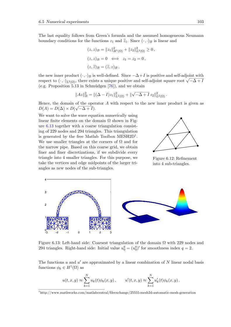
6.5 Numerical experiments 103
The last equality follows from Green’s formula and the assumed homogeneous Neumannboundary conditions for the functions z1 and z1. Since (· , ·)B is linear and
(z, z)B = ‖z1‖2H1(Ω) + ‖z2‖2L2(Ω) ≥ 0 ,
(z, z)B = 0 ⇐⇒ z1 = z2 = 0 ,
(z, z)B = (z, z)B ,
the new inner product (· , ·)B is well-defined. Since −∆+I is positive and self-adjoint withrespect to (· , ·)L2(Ω), there exists a unique positive and self-adjoint square root
√−∆ + I
(e.g. Proposition 5.13 in Schmudgen [76]), and we obtain
‖Az‖2B = ‖(∆− I)z1‖2L2(Ω) + ‖√−∆ + I z2‖2L2(Ω) .
Hence, the domain of the operator A with respect to the new inner product is given asD(A) = D(∆)×D(
√−∆ + I).
We want to solve the wave equation numerically usinglinear finite elements on the domain Ω shown in Fig-ure 6.13 together with a coarse triangulation consist-ing of 229 nodes and 294 triangles. This triangulationis generated by the free Matlab Toolbox MESH2D1.We use smaller triangles at the corners of Ω and forthe narrow pipe. Based on this coarse grid, we obtainfiner and finer discretizations, if we subdivide everytriangle into 4 smaller triangles. For this purpose, wetake the vertices and edge midpoints of the larger tri-angles as new nodes of the sub-triangles.
Figure 6.12: Refinementinto 4 sub-triangles.
Figure 6.13: Left-hand side: Coarsest triangulation of the domain Ω with 229 nodes and294 triangles. Right-hand side: Initial value uq0 = (uq0)′ for smoothness index q = 2.
The functions u and u′ are approximated by a linear combination of N linear nodal basisfunctions φk ∈ H1(Ω) as
u(t, x, y) ≈N∑k=1
uk(t)φk(x, y) , u′(t, x, y) ≈N∑k=1
u′k(t)φk(x, y) .
1http://www.mathworks.com/matlabcentral/fileexchange/25555-mesh2d-automatic-mesh-generation

104 6 Extended Krylov subspace approximation
In contrast to evolution equations with homogeneous Dirichlet boundary conditions, weadditionally have to take basis functions φk(x, y) ∈ H1(Ω) for the nodes on the boundary∂Ω. For every test function φk ∈ H1(Ω), the integral over ∂Ω in Green’s formula∫
Ωφk∆u d(x, y) = −
∫Ω∇φk∇u d(x, y) +
∫∂Ωφk∇nu ds
vanishes because of the prescribed homogeneous Neumann boundary conditions. Thisleads to the semi-discrete problem[
M OO M
] [v(t)w(t)
]′=
[O M
S −M O
] [v(t)w(t)
],
[v(0)w(0)
]=
[v0
w0
](6.9)
with initial values v0 =(uk(0)
)Nk=1
and w0 =(u′k(0)
)Nk=1
. The mass matrix M and thestiffness matrix S−M , which represents the discretization of ∆−I, consist of the L2-innerproducts
(M)ij = (φi, φj)L2(Ω) , (S)ij = −(∇φi,∇φj)L2(Ω) , i, j = 1, . . . , N .
Multiplying equation (6.9) from the left with the block diagonal matrix diag(M−1,M−1),the semi-discrete formulation reads
y′(t) =
[v(t)w(t)
]′=
[O I
M−1(S −M) O
] [v(t)w(t)
]= Ay(t) , y(0) = y0 =
[v0
w0
].
Since M and −S are symmetric positive definite, the same holds true for the composition−(S −M) of both matrices. Therefore, the positive definite and symmetric matrix
B =
[−(S −M) O
O M
],
corresponding to the operator counterpart B = diag(−∆ + I, I) from above, defines aninner product (· , ·)B on C2N by([
z1
z2
],
[z1
z2
])B
=[zH1 zH2
] [ −(S −M) OO M
] [z1
z2
]= −zH1 (S −M)z1 + zH2 Mz2 .
With respect to this inner product, we will show that W (A) ⊆ C−0 or, to be more precise,W (A) ⊆ iR. Thus, the matrix A fits in our framework above. This underlines theimportance to consider arbitrary inner products.
Lemma 6.8 For the inner product (· , ·)B, we have W (A) ⊆ iR or, respectively,
Re(Az, z)B = 0 for all z ∈ C2N .
Proof. For an arbitrary z = [zT1 , zT2 ]T ∈ C2N , a short calculation yields
(Az, z)B =
([O I
M−1(S −M) O
] [z1
z2
],
[z1
z2
])B
=
([z2
M−1(S −M)z1
],
[z1
z2
])B
= −zH1 (S −M)z2 + zH2 (S −M)z1 = 2i Im(zH2 (S −M)z1) ∈ iR .
This implies Re(Az, z)B = 0 and the lemma is proved. o

6.5 Numerical experiments 105
We now approximate the exact solution y(τ) of the semi-discrete problem at time τ in thepolynomial, the shift-and-invert, and the extended Krylov subspace by
y(τ) = eτAy0 ≈ eτAq+my0 = Vq+meτSq+mV H
q+mBy0 ,
where Vq+m ∈ CN×(q+m) is an orthonormal basis of the considered Krylov subspace oforder q + m. With the orthogonal projection Pq+m = Vq+mV
Hq+mB, the restriction of A
reads Aq+m = Pq+mAPq+m and the compression is given as Sq+m = V Hq+mBAVq+m. The
computation of Sq+m requires no calculation of M−1(S −M), since
BA =
[O −(S −M)
S −M O
].
The initial values uq0 and (uq0)′, whose index q refers to the abstract smoothness withrespect to the differential operator A, describe a peak in the right basin, each given bythe same function
g(x, y) =
(x− 1)2q+1(x− 3)2q+1y2q+1(y − 1)2q+1 , (x, y) ∈ [1, 3]× [0, 1] ,
0 , otherwise .
We normalize the vector [g, g]T with respect to the norm ‖ · ‖B associated to the innerproduct (· , ·)B with B = diag(−∆ + I, I). This means that we scale the vector [g, g]T bythe reciprocal of ∥∥[g, g]T
∥∥2
B=
∫Ω
(2g2 +∇g∇g
)d(x, y) .
By construction, yq0 = [g, g]T /‖[g, g]T ‖B belongs to D(Aq) but not to D(Aq+1). The cor-responding discrete initial value is designated by yq0 = [(vq0)T , (wq
0)T ]T = [(vq0)T , (vq0)T ]T
for vq0,wq0 ∈ CN .
On the basis of the considerations pre-sented in the previous Section 6.1, we plotin Figure 6.14 the quantities ‖A2y2
0‖B and‖A3y2
0‖B for different refinements of thetriangulation. The value 1 on the horizon-tal axis corresponds to the coarsest gridshown in Figure 6.13 and the values 2, 3, 4to the next three finer grids, that we ob-tain by subdividing each triangle into 4smaller sub-triangles, where the new tri-angles are created by joining nodes intro-duced at the edge midpoints. As expectedfrom the smoothness index q = 2, thenorm ‖A2y2
0‖B stays at the same level,whereas ‖A3y2
0‖B increases, if we refinethe spatial mesh.
1 2 3 40
1 · 103
2 · 103
3 · 103
‖A2y20‖B
‖A3y20‖B
Figure 6.14: Values ‖Ajy20‖, j = 2, 3,
for different refinements of the mesh.
In Figure 6.15, we draw the error curves for a coarse grid with 18 816 triangles and 10 057nodes for τ = 0.1, q = 1, 2 (left, right) and, in Figure 6.16, for a fine grid with 301 056triangles, 153 121 nodes (on the left) and 1 204 224 triangles, 607 297 nodes (on the right)for the parameters τ = 0.05 and q = 1. In the computations, the choice γ = 15 for the

106 6 Extended Krylov subspace approximation
shift has turned out to be advantageous with regard to the multigrid solver used for theapproximate solution of the linear systems in the rational Krylov decomposition.
The error curve for the approximation of eτAyq0 in the polynomial subspaceKγq+m,1(τA,yq0)is marked by a red dashed line, in the rational subspace Kγ1,q+m(τA,yq0) by a green dashed-dotted line and in the extended Krylov subspace Kγq+1,m(τA,yq0) by a blue solid line.As expected, the polynomial approximation virtually stagnates after q + 1 Krylov steps,whereas the errors of the extended and the rational Krylov subspace process exhibit asublinear convergence behavior.
0 5 10 15 2010−5
10−4
10−3
10−2
10−1
100 q = 1
0 5 10 15 2010−5
10−4
10−3
10−2
10−1
100 q = 2
Figure 6.15: Plot of the error ‖eτAyq0 − eτAq+myq0‖B versus the dimension of the Krylovsubspace for the standard Krylov subspace Kγq+m,1(τA,yq0) (red dashed line), the ratio-nal Krylov subspace Kγ1,q+m(τA,yq0) (green dash-dotted line), and the extended Krylovsubspace Kγq+1,m(τA,yq0) (blue solid line) for a coarse grid with 18 816 triangles, 10 057nodes, γ = 15, τ = 0.1, and smoothness indices q = 1, 2.
In the rational Krylov subspace decomposition, we have to solve linear systems of the form(γI − τA)x = vm, where vm = [(v1
m)T , (v2m)T ]T is the basis vector that is computed in
the mth iteration step. Noting that
(γI − τA)−1vm =
[γM −τM
−τ(S −M) γM
]−1 [M O
O M
][v1m
v2m
]
=
[ (γ2M − τ2(S −M)
)−1(γMv1
m + τMv2m)(
γ2M − τ2(S −M))−1
(τ(S −M)v1m + γMv2
m)
],
(6.10)
we have to solve two linear systems with the matrix(γ2M − τ2(S −M)
)−1and different
right-hand sides γMv1m + τMv2
m and τ(S −M)v1m + γMv2
m.
Since the matrices M and −(S −M) are both symmetric and positive definite, we canuse a standard geometric multigrid method which is based on the following idea (see, forinstance, Chapter V in [9]): Solving a large linear system Ax = b stemming from a spatialdiscretization, we first apply a smoother (e.g., Gauss-Seidel or damped Jacobi iteration)to some initial guess x0 of the solution x. This procedure removes high oscillations ofthe error vector x− x0 on the actual fine grid, whereas low frequencies are only reducedvery slowly. On that account, we change to a coarser grid, on which the low frequency
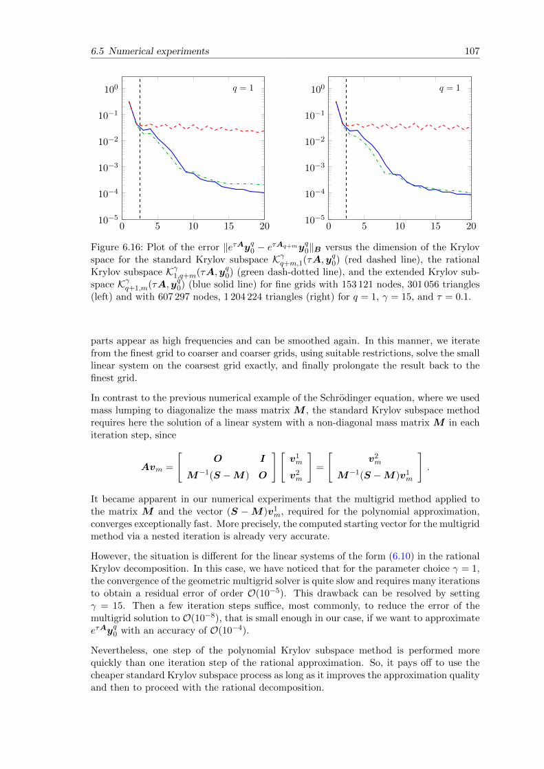
6.5 Numerical experiments 107
0 5 10 15 2010−5
10−4
10−3
10−2
10−1
100 q = 1
0 5 10 15 2010−5
10−4
10−3
10−2
10−1
100 q = 1
Figure 6.16: Plot of the error ‖eτAyq0 − eτAq+myq0‖B versus the dimension of the Krylovspace for the standard Krylov subspace Kγq+m,1(τA,yq0) (red dashed line), the rationalKrylov subspace Kγ1,q+m(τA,yq0) (green dash-dotted line), and the extended Krylov sub-space Kγq+1,m(τA,yq0) (blue solid line) for fine grids with 153 121 nodes, 301 056 triangles(left) and with 607 297 nodes, 1 204 224 triangles (right) for q = 1, γ = 15, and τ = 0.1.
parts appear as high frequencies and can be smoothed again. In this manner, we iteratefrom the finest grid to coarser and coarser grids, using suitable restrictions, solve the smalllinear system on the coarsest grid exactly, and finally prolongate the result back to thefinest grid.
In contrast to the previous numerical example of the Schrodinger equation, where we usedmass lumping to diagonalize the mass matrix M , the standard Krylov subspace methodrequires here the solution of a linear system with a non-diagonal mass matrix M in eachiteration step, since
Avm =
[O I
M−1(S −M) O
][v1m
v2m
]=
[v2m
M−1(S −M)v1m
].
It became apparent in our numerical experiments that the multigrid method applied tothe matrix M and the vector (S −M)v1
m, required for the polynomial approximation,converges exceptionally fast. More precisely, the computed starting vector for the multigridmethod via a nested iteration is already very accurate.
However, the situation is different for the linear systems of the form (6.10) in the rationalKrylov decomposition. In this case, we have noticed that for the parameter choice γ = 1,the convergence of the geometric multigrid solver is quite slow and requires many iterationsto obtain a residual error of order O(10−5). This drawback can be resolved by settingγ = 15. Then a few iteration steps suffice, most commonly, to reduce the error of themultigrid solution to O(10−8), that is small enough in our case, if we want to approximateeτAyq0 with an accuracy of O(10−4).
Nevertheless, one step of the polynomial Krylov subspace method is performed morequickly than one iteration step of the rational approximation. So, it pays off to use thecheaper standard Krylov subspace process as long as it improves the approximation qualityand then to proceed with the rational decomposition.

108 6 Extended Krylov subspace approximation
Computing for q = 2 and τ = 0.05 recursively y2k+1 ≈ eτAy2
k, k = 0, 1, . . ., with theextended Krylov method, we obtain an approximation to the exact solutions u(t) andu′(t) at time τ = 5 and τ = 10. In the first case, we iterate until m = 100 and, in thesecond case, we iterate until m = 200. The approximate solutions for u(5) and u(10) aredepicted in Figure 6.18 and Figure 6.19.
Furthermore, we want to illustrate what happens, if we use a “wrong” inner product forwhich the field of values ofA is not located in the left complex half-plane. For this purpose,we take the standard inner product for the finite-element discretization with respect tothe block diagonal matrix B = diag(M ,M) instead of B = diag(−(S −M),M) above.Then for arbitrary vectors 0 6= z = [zT1 , z
T2 ]T ∈ C2N , we have
(Az, z)B
(z, z)B
=1
(z, z)B
·(2i Im(zH1 Mz2) + zH2 Sz1
)⊆W
B(A) .
Choosing z in such a way that z1 = −z2, we can conclude that WB
(A) contains quantitiesin the right complex half-plane, since −S is positive definite. In Figure 6.17, we plot theapproximation error against the dimension of the Krylov subspace for the same parametersas in Figure 6.16, but using the “wrong” inner product with respect to B. In this case,no convergence can be observed anymore, regardless of whether we consider the extended,the shift-and-invert, or the polynomial Krylov subspace approximation.
0 10 20 30 40 5010−4
10−3
10−2
10−1
100
101
102
103
0 10 20 30 40 5010−2
10−1
100
Figure 6.17: Plot of the error ‖eτAyq0 − eτAq+myq0‖B versus the dimension of the Krylovsubspace for the standard Krylov subspace Kγq+m,1(τA,yq0) (red dashed line), the rationalKrylov subspace Kγ1,q+m(τA,yq0) (green dash-dotted line), and the extended Krylov sub-space Kγq+1,m(τA,yq0) (blue solid line) for the grid with 153 121 nodes, 301 056 triangles(left) and with 607 297 nodes, 1 204 224 triangles (right) for q = 1, γ = 15, τ = 0.1, andthe “wrong” inner product with respect to B = diag(M ,M).

6.5 Numerical experiments 109
Figure 6.18: Approximation to the exact solution u at time τ = 5.
Figure 6.19: Approximation to the exact solution u at time τ = 10.


Chapter 7
Rational Krylov subspace approximationwith simple poles
So far, we have concentrated on the shift-and-invert Krylov subspace method, a specialcase of the rational Krylov approximation, that uses only one single repeated pole atγ > 0. This chapter will focus on a rational Krylov method for the approximation ofϕ`(A)v, ` ≥ 1, taking different simple poles in the right complex half-plane. As before,we consider matrices A ∈ CN×N of arbitrary dimension N that satisfy the conditionW (A) ⊆ C−0 with respect to some inner product (· , ·) on the vector space CN .
In this chapter, we aim to speed-up the convergence of the Krylov approximation ofϕ`(A)v. Therefore, we choose 2m+ 1 equidistant poles zk ∈ C on the line Re(z) = γ > 0in the right complex half-plane. For this choice of poles, we will prove a faster convergencerate of order O(m−`). For comparison, we have seen that the error of the shift-and-invertKrylov subspace approximation behaves like O(m−`/2). Moreover, the resulting rationalKrylov process is easily parallelizable, since for different poles zk the 2m+1 linear systems(zkI − A)xk = v can be solved independently in parallel, which leads to an additionalspeed-up.
The following results are based on our preprint [24]. Before we turn to the analysis of therational Krylov subspace method with simple poles, we first need some preliminaries thatwe outline in the first section.
7.1 Preliminary notes
To guarantee the existence of (zkI −A)−1 under our assumption W (A) ⊆ C−0 , the poleszk of the rational Krylov subspace have to be located in the right complex half-plane. Wechoose 2m + 1 equidistant points zk = γ + ihk, k = −m, . . . ,m, with distance h on theline Re(z) = γ > 0 (cf. Figure 7.1) and consider the rational Krylov subspace
Q2m+2(A,v) =
r(A)v : r ∈ P2m+1
q2m+1
with the prescribed denominator polynomial
q2m+1(z) =
m∏k=−m
(zk − z) , zk = γ + ihk , k = −m, . . . ,m . (7.1)
By Lemma 4.9, this subspace can also be written as
Q2m+2(A,v) = span
v,
1
z−m −Av,
1
z−m+1 −Av, . . . ,
1
zm −Av
.

112 7 Rational Krylov subspace approximation with simple poles
z−m
z0
zm
h
γ
W (A)
Re
Im
Figure 7.1: Locus of W (A) and the roots zk of the denominator polynomial q2m+1.
Our first goal is to analyze the approximation of ϕ`(A) for ` ≥ 1 in the rational matrixsubspace
R2m+1(A) = span
r(A) : r ∈ P2m
q2m+1
.
We will establish uniform error estimates that hold true for matrices A with an arbitrarilylarge field of values in C−0 . Afterwards, these results will be used to bound the error‖ϕ`(A)v − ϕ`(Am)v‖ of the Krylov approximation. As before, Am = PmAPm is therestriction of A to Q2m+2(A,v), Pm denotes the orthogonal projector onto the rationalKrylov subspace, and Vm ∈ CN×(2m+2) contains an orthonormal basis [v1 v2 · · · v2m+2]of Q2m+2(A,v).
This basis Vm can be determined in parallel by assigning to every computing node thecalculation of xk = (zkI −A)−1v, that is required for the rational Krylov decomposition.This parallelization is possible by our choice of the poles leading to 2m+1 decoupled linearsystems for the 2m + 1 different poles zk, k = −m, . . . ,m. Subsequently, the computedsolutions xk are orthogonalized against each other to obtain an orthonormal basis of theKrylov subspace. As opposed to this, it is only possible to compute the basis of theshift-and-invert Krylov subspace with one fixed pole γ > 0 by a sequential process.
Whenever we write Q2m+2(A,v) or R2m+1(A), in what follows, we always mean therational subspace with the fixed denominator polynomial q2m+1 defined in (7.1).
In the following, we state a few definitions and lemmas, in order to lay a groundworkfor later examinations. The first lemma shows that the matrix exponential for arbitrarymatrices with a field of values in the left complex half-plane is bounded by one.
Lemma 7.1 For an arbitrary matrix A ∈ CN×N satisfying W (A) ⊆ C−0 and all τ ≥ 0,it holds
‖eτA‖ ≤ 1 .
Proof. (cf. LeVeque [51], p. 300) We consider the initial value problem u′(t) = Au(t) with

7.1 Preliminary notes 113
an arbitrary initial value u(0) = u0. By our assumption on W (A), we have
d
dt‖u(t)‖2 =
(u′(t),u(t)
)+(u(t),u′(t)
)=(Au(t),u(t)
)+(u(t),Au(t)
)= 2 Re
(Au(t),u(t)) ≤ 0
and thus ddt ‖u(t)‖ ≤ 0. It follows
‖eτAu0‖ = ‖u(τ)‖ ≤ ‖u(0)‖ = ‖u0‖ for any u0 ∈ CN .
As a consequence, the induced matrix norm of eτA is bounded by one. o
By equation (3.12), ϕ`(A) can be written as
ϕ`(A) =
∫ 1
0e(1−θ)A θ`−1
(`− 1)!dθ =
∫ 1
0esA
(1− s)`−1
(`− 1)!ds , ` ≥ 1 .
For our particular purposes, the representation
ϕ`(A) =
∫ ∞0
esA(1− s)`−1
(`− 1)!· 1[0,1](s) ds , ` ≥ 1 , (7.2)
is useful, which looks, at first sight, more complicated than the previous formula. But thisrepresentation of the matrix ϕ-functions provides the advantage that the rational matrixfunctions r(A) ∈ R2m+1(A) possess a similar integral representation.
Lemma 7.2 Every rational matrix function r(A) ∈ R2m+1(A) can be expressed as
r(A) =p2m(A)
q2m+1(A)=
m∑k=−m
ak1
γ + ihk −A=
∫ ∞0
esAm∑
k=−make−(γ+ihk)s ds ,
where q2m+1(z) =∏mk=−m(zk − z) with zk = γ + ihk, γ > 0.
Proof. The second equality follows directly from Lemma 4.9. In order to show the thirdequality, we first note that, by Lemma 7.1, we have
‖esAe−(γ+ihk)s‖ ≤ |e−γs|‖esA‖ ≤ e−γs for all s ≥ 0 .
Consequently, the improper Riemann integral∫∞
0 esAe−(γ+ihk)s ds exists and we conclude
that lims→∞ esAe−(γ+ihk)s = O. This yields∫ ∞
0esAe−(γ+ihk)s ds = − 1
γ + ihk −AesAe−(γ+ihk)s
∣∣∣∞0
=1
γ + ihk −A(7.3)
and therefore∫ ∞0
esAm∑
k=−make−(γ+ihk)s ds =
m∑k=−m
ak
∫ ∞0
esAe−(γ+ihk)s ds =
m∑k=−m
ak1
γ + ihk −A
as claimed above. o

114 7 Rational Krylov subspace approximation with simple poles
Comparing equation (7.3) with the general formula of the Laplace transform, which is fora function f : [0,∞)→ C defined as
Lf(t) =
∫ ∞0
f(s)e−ts ds ,
the inverse (zkI −A)−1 can be understood as the Laplace transform of f(s) = esA at thepoint t = zk = γ + ihk (e.g., [40], Section 11.1). In this context, the parameter γ > 0causes an exponential damping that will be relevant for later purposes.
We have already seen above that if W (A) ⊆ C−0 , the same holds true for τA, that is,W (τA) ⊆ C−0 for τ ≥ 0. Without loss of generality, we thus state our theorems in thefollowing for τ = 1. All subsequent results remain valid for τA, the matrix A has just tobe replaced by the scaled matrix τA everywhere.
The estimate for the best approximation of ϕ`(A) in the subspace R2m+1(A) will lead toa problem of best trigonometric approximation in the space L1 on the unit circle T. Werefer to T as the real numbers with the identification of points modulo 2π, and the spaceL1(T) consists of all 2π-periodic functions satisfying
∫T |f(s)| ds <∞. To bound the error
of the approximation problem on L1(T), we will need a similar modulus of smoothness asin Chapter 5 and the concept of bounded variation. Following [14], we state the followingtwo definitions.
Definition 7.3 A 2π-periodic function f is of bounded variation on the unit circle T, orin short notation f ∈ BV (T), if
VarTf := supn−1∑i=1
|f(xi+1)− f(xi)| <∞ ,
where the supremum is taken over all partitions x1 < x2 < . . . < xn, xi ∈ T, i = 1, . . . , n.
Functions of bounded variation can have a countable number of discontinuities αi, wherebythe left and right limits, limsαi f(s) and limsαi f(s), have to exist at each point αi. Fur-thermore, we will require the modified variation Var∗T f , which is defined as the variationof a correction f∗ of the function f . This corrected function f∗ coincides with f exceptfor the points αi of discontinuity.
Definition 7.4 For f ∈ BV (T) with a countable set of discontinuities αi, we define
Var∗T f := VarT f∗ ,
where the corrected function f∗ is some function that coincides with f on T\⋃iαi and
takes values between limsαi f(s) and limsαi f(s) at the points αi of discontinuity.
With this newly defined variation, we can bound the rth modulus of smoothness ωr(f, δ)L1(T)
with respect to the space L1(T),
ωr(f, δ)L1(T) := sup0<h≤δ
∫T|∆r
h(f, t)| dt , ∆rh(f, t) =
r∑k=0
(r
k
)(−1)r−kf(t+ kh) ,
for a function f ∈ L1(T) (see [14], Theorem 9.3 in Chapter 2 on page 53 for p = 1). Thismodulus of smoothness has already been used in Section 5.4, cf. equation (5.14), for themaximum norm.

7.2 Error bounds 115
Lemma 7.5 Let f ∈ L1(T) be a 2π-periodic function which can be corrected on a set ofmeasure zero to a function g such that g(r−2) is absolutely continuous and the generalized(weak) derivative g(r−1) is of bounded variation on T. Then the estimate
ωr(f, δ)L1(T) ≤ δr Var∗T g(r−1) , δ > 0
holds true.
The Stechkin inequality, obtained in the next lemma, enables us to bound the best ap-proximation of a function f ∈ L1(T) by a trigonometric polynomial using the rth modulusof smoothness of f (see [14], Theorem 2.3 in Chapter 7 for the case p = 1).
Lemma 7.6 For r = 1, 2, . . . and a 2π-periodic functions f ∈ L1(T), there exists a con-stant C(r) such that
Em(f) := infP∈Tm
∫T|f(s)− P (s)| ds ≤ C(r)ωr
(f,
1
m
)L1(T)
,
where Tm denotes the set of all trigonometric polynomials of degree m with functions ofthe form
P (s) =α0
2+
m∑k=1
αk cos(ks) + βk sin(ks) , αk, βk ∈ R .
Since Tm is a finite dimensional space, there exists an element P ∗ ∈ Tm of best approxi-mation for which the infimum in Em(f) is attained.
Herewith, all key requirements for the estimate of ‖ϕ`(A)− r(A)‖ for r(A) ∈ R2m+1(A)in the next section are provided.
7.2 Error bounds
The first theorem in this section states an upper bound for the best approximation ofϕ`(A), ` ≥ 1, in the rational matrix space
R2m+1(A) =
r(A) : r ∈ P2m
q2m+1
, q2m+1(z) =
m∏k=−m
(zk − z) ,
where the poles zk are given, as mentioned above, by zk = γ+ ihk for k = −m, . . . ,m andshift γ > 0.
Theorem 7.7 Let A be a matrix with W (A) ⊆ C−0 . Then for the best approximation ofthe matrix function ϕ`(A) for ` ≥ 1 in the subspace R2m+1(A), it holds
infr∈ P2m
q2m+1
‖ϕ`(A)− r(A)‖ ≤ C1(`, γ)e−
γπh
1− e−2γπh
+ C2(`, γ)1
(hm)`, (7.4)
where the constants C1 and C2 depend only on γ and `.

116 7 Rational Krylov subspace approximation with simple poles
Proof. With the auxiliary results in Section 7.1, we are able to reduce the approximationproblem on CN×N to a one-dimensional problem on the right semi-axis [0,∞). Splittingthis one-dimensional problem into two appropriate subproblems on two disjoint subinter-vals of [0,∞), we finally obtain the two different terms on the right hand-side of the bound(7.4). In this bound, the second term arises from a trigonometric approximation on a finitespectrum and the first term is obtained due to the exponentially damping of the Laplacetransform in (7.3), caused by the shift γ.
We first note that via partial fraction expansion, cf. Lemma 4.9, we have
infr∈ P2m
q2m+1
‖ϕ`(A)− r(A)‖ = infak
∥∥∥∥∥ϕ`(A)−m∑
k=−mak
1
γ + ihk −A
∥∥∥∥∥ .Using the integral representation of ϕ`(A) in (7.2) and of the rational function r(A) inLemma 7.2 as well as the inequality ‖esA‖ ≤ 1 in Lemma 7.1, the following one-dimensio-nal expression is obtained:∥∥∥∥∥ϕ`(A)−
m∑k=−m
ak1
γ + ihk −A
∥∥∥∥∥ ≤∫ ∞
0‖esA‖
∣∣∣∣∣1[0,1](s)(1− s)`−1
(`− 1)!−
m∑k=−m
ake−(γ+ihk)s
∣∣∣∣∣ ds≤∫ ∞
0
∣∣∣∣∣1[0,1](s)(1− s)`−1
(`− 1)!−
m∑k=−m
ake−(γ+ihk)s
∣∣∣∣∣ ds .For the rest of the proof, we always assume that the distance h between the equidistantpoles zk is chosen such that h < π, which implies that π
h > 1. Now, the last integral issplitted into
∫ ∞0
∣∣∣∣∣1[0,1](s)(1− s)`−1
(`− 1)!−
m∑k=−m
ake−(γ+ihk)s
∣∣∣∣∣ ds=
∫ πh
0
∣∣∣∣∣1[0,1](s)(1− s)`−1
(`− 1)!−
m∑k=−m
ake−(γ+ihk)s
∣∣∣∣∣ ds+
∫ ∞πh
∣∣∣∣∣m∑
k=−make−(γ+ihk)s
∣∣∣∣∣ ds (7.5)
=
∫ πh
0
∣∣∣∣∣1[0,1](s)(1− s)`−1
(`− 1)!−
m∑k=−m
ake−(γ+ihk)s
∣∣∣∣∣ ds+∞∑j=1
∫ (2j+1)πh
(2j−1)πh
∣∣∣∣∣m∑
k=−make−(γ+ihk)s
∣∣∣∣∣ ds .In order to exploit the results for the best trigonometric approximation on L1(T) in theprevious section, the first term, involving the indicator function 1[0,1](s), must be extendedto the interval [−π
h ,πh ) in a suitable way. A change of variables then leads to the required
domain T = [−π, π) of integration. For this purpose, we have to find a new function thatcoincides with 1[0,1](s)(1−s)`−1/(`−1)! on [0, πh ) and that has sufficient smoothness prop-erties. The last requirement is to guarantee a best possible trigonometric approximation.With regard to this, we define the function
g(s) :=
C
∫ s
−1e− 1
1−(2t+1)2 dt , −1 < s < 0 ,
1 , s ≥ 0 ,
0 , s ≤ −1
(7.6)

7.2 Error bounds 117
with C = (∫ 0−1 e
− 1
1−(2t+1)2 dt)−1. This function g is infinitely many times differentiable,that is, g ∈ C∞(R). Furthermore, we set
f`(s) := g(s) · eγs · 1[−1,1](s)(1− s)`−1
(`− 1)!∈ C`−2(R) .
This newly defined function belongs to C∞(R\1) and has a weak derivative of order`− 1 (see Figure 7.2 for ` = 3).
−1 1
0.3
f3
−1 1
0.5
−0.5
f ′3
−1 1
5f ′′3
Figure 7.2: Plot of f3, f ′3, and the weak derivative f ′′3 with jump discontinuity at 1.
Since g(s) = 1 for s ≥ 0, it follows∫ πh
0
∣∣∣∣∣1[0,1](s)(1− s)`−1
(`− 1)!−
m∑k=−m
ake−(γ+ihk)s
∣∣∣∣∣ ds=
∫ πh
0
∣∣∣∣∣e−γseγs · g(s) · 1[0,1](s)(1− s)`−1
(`− 1)!−
m∑k=−m
ake−γse−ihks
∣∣∣∣∣ ds=
∫ πh
0e−γs
∣∣∣∣∣f`(s)−m∑
k=−make−ihks
∣∣∣∣∣ ds ≤∫ π
h
0
∣∣∣∣∣f`(s)−m∑
k=−make−ihks
∣∣∣∣∣ ds≤∫ π
h
−πh
∣∣∣∣∣f`(s)−m∑
k=−make−ihks
∣∣∣∣∣ ds .The coefficients a−m, . . . , am are now chosen according to the best approximation for f`(s)in the space Tm of all real trigonometric polynomials of degree m. This leads to∫ π
h
−πh
∣∣∣∣∣f`(s)−m∑
k=−make−ihks
∣∣∣∣∣ ds = minbk
∫ πh
−πh
∣∣∣∣∣f`(s)−m∑
k=−mbke−ihks
∣∣∣∣∣ ds=
1
h·minbk
∫ π
−π
∣∣∣∣∣f` ( sh)−m∑
k=−mbke−iks
∣∣∣∣∣ ds =1
h· Em
(f`
( ·h
)),
(7.7)
if the real function f`(·h)∣∣T is extended periodically to a function in L1(T). Since the best
approximation of a real function has to be real as well, the complex coefficients ak haveto be taken in such a way that a−k = ak. Then we have
ake−iks + a−ke
iks = 2 Re(ak) cos(ks) + 2 Im(ak) sin(ks)

118 7 Rational Krylov subspace approximation with simple poles
and∑m
k=−m ake−iks is a real trigonometric polynomial. The application of Lemma 7.6
now yields
Em
(f`
( ·h
))≤ C(r)ωr
(f`
( ·h
),
1
m
)L1(T)
.
The (`−2)nd derivative of f`(·h) is absolutely continuous and the (`−1)st weak derivative
is of bounded variation on T. Hence, we are able to apply Lemma 7.5 with r equal to `,to obtain
ωr
(f`
( ·h
),
1
m
)L1(T)
≤ 1
m`Var∗T f
(`−1)`
( ·h
)=
1
m`VarT
(f
(`−1)`
( ·h
))∗=:
1
m`VarT u`(·) ,
where
u`(·) =(f
(`−1)`
( ·h
))∗=
(d`−1
ds`−1
[f`
( ·h
)])∗∈ BV (T) .
According to Definition 7.4, the function u`(·) is a suitable correction of the function
f(`−1)` ( ·h) with jump discontinuity at h. In our case, we choose
u`(s) :=
f
(`−1)`
( sh
), s ∈ T\h ,
1
2
(limsh
f(`−1)`
( sh
)+ limsh
f(`−1)`
( sh
)), s = h .
Moreover, we define the transformed function
u`(s) :=
f
(`−1)` (s) , s ∈
[−πh ,
πh
)\1 ,
1
2
(lims1
f(`−1)` (s) + lim
s1f
(`−1)` (s)
), s = 1 ,
which does no longer depend on h. Due to the definition of f`(s), the function u`(s) isequal to zero for s ≤ −1 and s > 1. With the chain rule we obtain
VarT u`(·) =1
h`−1Var[−π
h,πh
)u`(·) =1
h`−1Var[−1,1]u`(·) .
Altogether, we have
∫ πh
−πh
∣∣∣∣∣f`(s)−m∑
k=−make−ihks
∣∣∣∣∣ ds ≤ C2(`, γ)1
(hm)`, C2(`, γ) = C(`)Var[−1,1]u`(·) ,
where the property u`(·) ∈ BV (T) assures that C2(`, γ) <∞. Consequently, the first termin (7.5) is covered. Our next task is to bound the second term. As mentioned above, wewill take advantage of the fact that the parameter γ in the exponential function leads toa damping in the remaining domain of integration. Noting that
e−γs ≤ e−γ(2j−1)πh for s ∈
[(2j − 1)
π
h, (2j + 1)
π
h
], j = 1, 2, . . . ,

7.2 Error bounds 119
we conclude by the periodicity of eihks and the geometric series that
∞∑j=1
∫ (2j+1)πh
(2j−1)πh
∣∣∣∣∣m∑
k=−make−(γ+ihk)s
∣∣∣∣∣ ds ≤∞∑j=1
e−γ(2j−1)πh
∫ (2j+1)πh
(2j−1)πh
∣∣∣∣∣m∑
k=−make−ihks
∣∣∣∣∣ ds= eγ
πh
( ∞∑j=0
(e−2γ π
h
)j− 1
)·∫ π
h
−πh
∣∣∣∣∣m∑
k=−make−ihks
∣∣∣∣∣ ds=
e−γπh
1− e−2γ πh
·∫ π
h
−πh
∣∣∣∣∣m∑
k=−make−ihks
∣∣∣∣∣ ds .The integral term can be estimated by exploiting that the coefficients a−m, . . . , am havebeen chosen in (7.7) according to the best approximation. This gives∫ π
h
−πh
∣∣∣∣∣m∑
k=−make−ihks
∣∣∣∣∣ ds =
∫ πh
−πh
∣∣∣∣∣m∑
k=−make−ihks − f`(s) + f`(s)
∣∣∣∣∣ ds≤∫ π
h
−πh
|f`(s)| ds + minbk
∫ πh
−πh
∣∣∣∣∣f`(s)−m∑
k=−mbke−ihks
∣∣∣∣∣ ds≤ 2
∫ πh
−πh
|f`(s)| ds ,
if we set b−m = . . . = bm = 0. Inserting the definition of f`, we get∫ πh
−πh
|f`(s)| ds =
∫ πh
−πh
∣∣∣∣g(s) · eγs · 1[−1,1](s)(1− s)`−1
(`− 1)!
∣∣∣∣ ds≤ eγ
∫ 1
−1
∣∣∣∣(1− s)`−1
(`− 1)!
∣∣∣∣ ds ≤ eγ 2`
`!.
Thus, the second term in (7.5) fulfills the inequality
∞∑j=1
∫ (2j+1)πh
(2j−1)πh
∣∣∣∣∣m∑
k=−make
(−γ−ihk)s
∣∣∣∣∣ ds ≤ C1(`, γ)e−γ
πh
1− e−2γ πh
, C1(`, γ) = eγ2`+1
`!.
Finally, we obtain the desired error bound. o
The assumption h < π in the proof of Theorem 7.7 is not mandatory. Just as well, wecan choose another condition for the distance h between the simple poles zk = γ + ihk.Then we need a suitable change of variables in the proof, in order to end up again with atrigonometric approximation problem on L1(T).
The attentive reader may have recognized that we just considered the approximationof ϕ`(A) in the space R2m+1(A), containing all rational matrix functions of the formp2m(A)/q2m+1(A) with p2m ∈ P2m, whereas we are finally interested in an approximationof ϕ`(A)v in the Krylov subspace
Q2m+2(A,v) =
r(A)v : r ∈ P2m+1
q2m+1
,

120 7 Rational Krylov subspace approximation with simple poles
whose numerator polynomial p2m+1 has a degree one larger than in the space R2m+1(A).Compared to the subspace R2m+1(A)v = P2m(A)/q2m+1(A)v, one could say that therational Krylov subspace Q2m+2(A,v) contains in addition the vector v. This additionalvector is required to ensure that the condition r(A)v = r(Am)v holds for every rationalfunction r ∈ P2m/q2m+1, where Am = PmAPm and Pm is the orthogonal projectiononto Q2m+2(A,v). In particular, this requirement necessitates that Pmv = v, which isonly fulfilled if v is an element of the considered Krylov subspace. The following simpleexample illustrates this claim.
We consider r(z) = 1γ−z ∈ P2m/q2m+1 and assume that Pm is the orthogonal projection
onto R2m+1(A)v. The requirement r(A)v = r(Am)v is then equivalent to
1
γ −Av =
1
γ − PmAPmv
⇐⇒ (γI − PmAPm)1
γ −Av =
γ
γ −Av − Pm
A
γ −Av = v
⇐⇒ γ
γ −Av + Pm
(I − γ
γ −A
)v = Pmv = v ,
showing that Pmv = v has to be fulfilled.
Due to the relation
R2m+1(A)v + spanv =P2m(A)
q2m+1(A)v + spanv =
P2m+1(A)
q2m+1(A)v = Q2m+2(A,v) ,
we study, from now on, the approximation of ϕ`(A)v by ϕ`(Am) for ` ≥ 1, where Am
is the restriction of A to the rational Krylov subspace Q2m+2(A,v). With the help ofTheorem 7.7, we are able to bound the best approximation of ϕ`(A)v in the subspaceR2m+1(A)v. This raises the question whether Theorem 7.7 can nevertheless be appliedfor the approximation of ϕ`(A)v in Q2m+2(A,v). The answer to this question is yes: SinceP2m/q2m+1 ⊂ P2m+1/q2m+1, adding the vector v to the subspace causes no problem.
Theorem 7.8 Let the matrix A satisfy W (A) ⊆ C−0 and let Am = PmAPm be therestriction of A to Q2m+2(A,v) via orthogonal projection. Then the error of the rationalKrylov subspace approximation can be bounded by
‖ϕ`(A)v − ϕ`(Am)v‖ ≤ 2
[C1(`, γ)
e−γπh
1− e−2γπh
+ C2(`, γ)1
(hm)`
]‖v‖ ,
where C1 and C2 are the same constants as in Theorem 7.7.
Proof. By Lemma 4.12, the Krylov subspace approximation in Q2m+2(A,v) is exact forevery rational function r ∈ P2m+1/q2m+1, where q2m+1(z) =
∏mk=−m(γ + ihk − z). With
r(A)v = r(Am)v, it follows
‖ϕ`(A)v − ϕ`(Am)v‖ ≤ ‖ϕ`(A)− r(A)‖‖v‖+ ‖ϕ`(Am)− r(Am)‖‖v‖
for all r ∈ P2m+1/q2m+1. We pick this rational function r especially from the spaceP2m/q2m+1 ⊆ P2m+1/q2m+1 and use the already known relation W (Am) ⊆W (A) ⊆ C−0 .
7.3 Choice of the parameters γ and h 121
In this case, we are able to estimate both terms on the right hand-side as in the proof ofTheorem 7.7. This gives
‖ϕ`(A)v − ϕ`(Am)v‖ ≤ 2‖v‖∫ ∞
0
∣∣∣∣∣1[0,1](s)(1− s)`−1
(`− 1)!−
m∑k=−m
ake−(γ+ihk)s
∣∣∣∣∣ ds .From here, the estimate of the one-dimensional approximation problem proceeds analo-gously to the proof of Theorem 7.7 and we end up with
‖ϕ`(A)v − ϕ`(Am)v‖ ≤ 2
[C1(`, γ)
e−γπh
1− e−2γπh
+ C2(`, γ)1
(hm)`
]‖v‖ ,
which concludes the proof. o
If the first term of the error bound in Theorem 7.8 is small enough, the second term pre-dicts a sublinear convergence behavior of order O
((hm)−`
). The obtained error bound is
completely independent of the matrix A and therefore guarantees a uniform approxima-tion for arbitrary matrices whose field of values is located somewhere in the left complexhalf-plane. In the case that A represents a spatial discretization matrix of a differentialoperator, we proved a convergence rate that is entirely independent of the chosen meshsize and the refinement of the grid.
It has to be taken into account that only the second term of our error bound decreaseswith the dimension of the Krylov subspace. In order to obtain an efficient and usefulerror estimate, it is of great importance that the occurring free parameters are reasonablychosen. In contrast to the shift-and-invert and the extended Krylov subspace method,where we use a single repeated pole γ, we not only have to think about a suitable choice ofthe shift γ, but also about an appropriate selection for the distance h between the differentpoles of our rational Krylov subspace method. This will be the content of the next section.
7.3 Choice of the parameters γ and h
In this section, we want to investigate suitable choices for the free parameters γ and h.To this end, let us recall that the error for the approximation of ϕ`(A)v in the rationalKrylov subspace Q2m+2(A,v) behaves like
‖ϕ`(A)v − ϕ`(Am)v‖ ≤ 2
[C1(`, γ)
e−γπh
1− e−2γπh
+ C2(`, γ)1
(hm)`
]‖v‖ .
For the subsequent discussion, we have to understand in what way the two occurringconstants C1(`, γ) and C2(`, γ) depend on γ. Looking back to the proof of Theorem 7.7,we already know that
C1(`, γ) = eγ2`+1
`!, C2(`, γ) = C(`)Var[−1,1]u`(·) ,
where u`(s) was defined as f(`−1)` (s) for s ∈ [−π
h ,πh )\1 and as the mean of the left and
right limit of f(`−1)` (s) on the jump at the point 1. Hereby, the function f` was given as
f`(s) = g(s) · eγs · 1[−1,1](s)(1− s)`−1
(`− 1)!∈ C`−2(R)

122 7 Rational Krylov subspace approximation with simple poles
with the auxiliary function g defined in (7.6). To estimate the variation of u`, we exploitthe fact that u` is only supported on [−1, 1] and differentiable on [−1, 1). Moreover, it iswell-known that for a function f , which is differentiable on [a, b], we have
Var[a,b] f(·) =
∫ b
a|f ′(s)| ds
(for instance, [68], Section 16.1). This leads to the inequality
Var[−1,1]u`(·) ≤∫ 1
−1|f (`)` (s)| ds+ sup
s∈[−1,1)|f (`−1)` (s)| ,
where the last term is required to cover the jump discontinuity of u` at 1. Hence, we are
now concerned with the estimate of |f (`−1)` (s)| as well as |f (`)
` (s)| for s ∈ [−1, 1). For thefunction g in (7.6), we define the constant
Cg := maxk=0,...,`
maxs∈[−1,1]
|g(k)(s)| <∞ ,
which is independent of γ, since g itself does not depend on γ. The general Leibniz ruleyields
|f (`−1)` (s)| =
∣∣∣∣∣`−1∑k=0
(`− 1
k
)g(`−1−k)(s)
(eγs
(1− s)`−1
(`− 1)!
)(k)∣∣∣∣∣
≤ Cg ·`−1∑k=0
(`− 1
k
) ∣∣∣∣∣(eγs
(1− s)`−1
(`− 1)!
)(k)∣∣∣∣∣ , s ∈ [−1, 1) .
Using the Leibniz rule once more, we obtain∣∣∣∣∣(eγs
(1− s)`−1
(`− 1)!
)(k)∣∣∣∣∣ ≤
k∑j=0
(k
j
) ∣∣∣(eγs)(k−j)∣∣∣ ∣∣∣∣∣(
(1− s)`−1
(`− 1)!
)(j)∣∣∣∣∣ ≤ 2 eγ(1 + γ)k
by the binomial identity. The last inequality follows from the fact that∣∣( (1−s)`−1
(`−1)!
)(j)∣∣ ≤ 2
for all j = 0, . . . , k, ` ≥ 1, and s ∈ [−1, 1). Then a further application of the binomialidentity provides the bound
|f (`−1)` (s)| ≤ 2Cge
γ ·`−1∑k=0
(`− 1
k
)(1 + γ)k = 2Cge
γ(2 + γ)`−1 .
An analogous estimate for the second term |f (`)` (s)| yields |f (`)
` (s)| ≤ 2Cgeγ(2 + γ)`.
Altogether, this gives
Var[−1,1]u`(·) ≤∫ 1
−12Cge
γ(2 + γ)` ds+ 2Cgeγ(2 + γ)`−1 ≤ 6Cge
γ(2 + γ)`
and thus
C2(`, γ) = C(`)Var[−1,1]u`(·) ≤ C(`)eγ(2 + γ)`
with a constant C(`) that depends only on `.

7.3 Choice of the parameters γ and h 123
We are now prepared to discuss suitable choices for γ and h, by taking the whole expression
C1(`, γ)e−
γπh
1− e−2γπh
+ C2(`, γ)1
(hm)`≤ 2`+1
`!
eγ(1−πh
)
1− e−2γπh
+ C(`) eγ(2 + γ)`1
(hm)`(7.8)
into account. We first observe that the shift γ > 0 should neither be chosen too small nortoo large, since otherwise either the first or the second term in (7.8) becomes quite large.Apart from this, a suitable choice for h is also not obvious. What is certain is that theparameter h is restricted by 0 < h < π, in accordance with the assumption in the proofof Theorem 7.7.
The first term in (7.8) is independent of the iteration index and therefore does not decreasewith m. A first possibility for the choice of the two parameters might be to define h andγ in such a way that
C1(`, γ)e−
γπh
1− e−2γπh
≤ tol ,
where tol is a given tolerance, e.g., tol = 10−4. We should avoid very small values for h,since the second term in (7.8) is of order O(h−`). Furthermore, we would have to expect in-stability problems in the orthogonalization process of the parallel rational Krylov subspacedecomposition for small h, since (zkI −A)−1v ≈ (zk+1I −A)−1v. This stability problemcan be overcome by using the serial rational Arnoldi decomposition in Algorithm 4.10 orthe rational Krylov subspace procedure by Ruhe. On the other hand, values of h greaterthan one unfortunately imply that the prefactor eγ(2 + γ)` of the second term is quitelarge. For the case ` = 1, the correlation between h, γ, and eγ(2 + γ)` is demonstrated inthe following table:
C1(`, γ) e−γπh
1−e−2γπh
h γ eγ(2 + γ)
≤ 10−4 0.25 ≥ 1 ≥ 8.2
≤ 10−4 0.5 ≥ 2.1 ≥ 33.5
≤ 10−4 1 ≥ 5 ≥ 1038.9
≤ 10−4 2 ≥ 18.6 ≥ 2.5 · 109
Table 7.1: Correlation between h, γ, and eγ(2 + γ)` for ` = 1.
A second possible strategy is to choose a fixed γ of moderate size, for example γ = 1, andto select h such that both terms in (7.8) equally decrease with the dimension m of therational Krylov subspace. For this, we have to solve the equation e−γπ/h = (hm)−` for h.If we rearrange this expression in a suitable way, we have
e−γπh =
1
(hm)`⇐⇒ (hm)` =
(eγπh`
)`⇐⇒ hm = e
γπh`
⇐⇒ γπm
`=γπ
h`eγπh` . (7.9)

124 7 Rational Krylov subspace approximation with simple poles
At this point, the so-called Lambert W -function W (z) comes into play. It is given asthe inverse function of f(x) = xex = z and therefore provides a solution of the equationz = W (z)eW (z). Identifying z with γπm
` and W (z) with γπh` in (7.9), the relation
W(γπm
`
)=γπ
h`or h =
γπ
`
1
W(γπm
`
) (7.10)
is obtained. Using the well-known estimate (cf. [35])
ln(z)− ln(
ln(z))≤W (z) ≤ ln(z) , z ≥ e , z ∈ R ,
we find for h = γπ` W
(γπm`
)−1the estimates
e−γπh = e−`W( γπm` ) ≤ e−`[ln( γπm` )−ln(ln( γπm` ))] =
(`
γπm
)(ln(γπm
`
))= O
(ln(m)`
m`
)and
1
(hm)`=
(`
γπm
)`W `(γπm
`
)≤(
`
γπm
)` (ln(γπm
`
))= O
(ln(m)`
m`
).
Consequently, the terms in (7.8) behave like
C1(`, γ)e−
γπh
1− e−2γπh
+ C2(`, γ)1
(hm)`≤ C(`, γ)
(ln(m)
m
)`. (7.11)
7.4 Comparison with a fixed rational approximation
This section draws a comparison between the approximation of ϕ`(A)v, ` ≥ 2, in therational Krylov subspace Q2m+2(A,v) and a fixed rational approximation using the samepoles zk = γ + ihk, that is,
ϕ`(A)v ≈m∑
k=−m
ckzk −A
v
with given coefficients c−m, . . . , cm ∈ C. Such a fixed approximation is obtained with thehelp of the ideas in Stenger [80] as well as Lopez-Fernandez and Palencia [53] applied tothe following useful representation of the ϕ`-functions by the Cauchy integral formula.
Lemma 7.9 For ` ≥ 2 and z ∈ C−0 , we have
ϕ`(z) =1
2πi
∫Γ
eξ
ξ`1
ξ − zdξ ,
where Γ is a curve with parametrization Γ(t) = γ + it, γ > 0, and the parameter t ∈ Rruns from −∞ to +∞.
Proof. We use the representation
ϕ`(z) =ez
z`−
`−1∑k=0
zk−`
k!, ϕ`(0) =
1
`!,

7.4 Comparison with a fixed rational approximation 125
for the ϕ`-functions, cf. relation (3.13). Since ϕ` is analytic in C, the Cauchy integralformula yields
ϕ`(z) =1
2πi
∫Γ
eξ
ξ`1
ξ − zdξ − 1
2πi
∫Γ
`−1∑k=0
ξk−`
k!
1
ξ − zdξ , (7.12)
where Γ is a simple closed rectifiable curve with winding number one around z ∈ C−0 . For
the contour Γ, we take particularly the boundary Γ1 + Γ2 of the left semicircle of the diskwith center point γ > 0 and radius R > 0, which is parametrized by
Γ1(t) = γ + it , t ∈ [−R,R] , Γ2(t) = γ +Reit , t ∈(π
2,3π
2
),
such that z ∈ int(Γ) = int(Γ1 + Γ2). Using the residue theorem, we see that the secondterm on the right-hand side of (7.12) vanishes. Moreover, it is easy to verify that
limR→∞
1
2πi
∫Γ2
eξ
ξ`1
ξ − zdξ = 0 .
Since, for ` ≥ 2, we have
limR→∞
∣∣∣∣∫Γ1
eξ
ξ`1
ξ − zdξ
∣∣∣∣ ≤ limR→∞
∫ R
−R
eγ
|γ + it|`1
|γ + it− z|dt ≤ eγ
γ
∫ ∞−∞
1
|γ + it|`dt <∞ ,
the improper integral over Γ1 exists and the desired statement of the lemma is provedwith Γ(t) = Γ1(t) for t ∈ R. o
The limit
limt→±∞
eγ+it
(γ + it)`1
γ + it− z= 0
of the integrand in Lemma 7.9 suggests an approximation of ϕ`(z) by the application of atruncated trapezoidal rule with step size h to the integral representation. More precisely,we consider the approximation
ϕ`(z) ≈h
2π
m∑k=−m
eγ+ihk
(γ + ihk)`1
γ + ihk − z=: Sm(ϕ`, h, z) ,
where Sm(ϕ`, h, z) is a rational function with the same poles zk = γ+ihk as in our rationalKrylov subspace method above. The quadrature error of this approach will be estimatedin the next lemma.
Lemma 7.10 The error of the truncated trapezoidal rule applied to the integral represen-tation of ϕ`(z), ` ≥ 2, in Lemma 7.9 is for all z ∈ C−0 bounded by
|ϕ`(z)− Sm(ϕ`, h, z)| ≤ C1(`, γ)1
e2πdh − 1
+ C2(`, γ)1
(hm)`−1, 0 < d < γ . (7.13)
Proof. The proof follows the ideas of the proof of Theorem 1 given in [53]. First, we set
g(t) :=eγ+it
(γ + it)`1
γ + it− z.

126 7 Rational Krylov subspace approximation with simple poles
Then we estimate∣∣∣∣∣∫ ∞−∞
g(t) dt− hm∑
k=−mg(kh)
∣∣∣∣∣ =
∣∣∣∣∣∣∫ ∞−∞
g(t) dt− h∞∑
k=−∞g(kh) + h
∑|k|≥m+1
g(kh)
∣∣∣∣∣∣≤
∣∣∣∣∣∫ ∞−∞
g(t) dt− h∞∑
k=−∞g(kh)
∣∣∣∣∣+ h∑
|k|≥m+1
|g(kh)| .
The first term satisfies the assumptions of Theorem 4.1 in [80] and can be bounded by∣∣∣∣∣∫ ∞−∞
g(t) dt− h∞∑
k=−∞g(kh)
∣∣∣∣∣ ≤ C(g, d)
e2πdh − 1
, 0 < d < γ .
A calculation of the second term gives
h∑
|k|≥m+1
|g(kh)| = h∑
k≥m+1
(|g(kh)|+ |g(−kh)|
)≤ 2h
eγ
γ
∞∑k=m+1
1
|γ + ihk|`
≤ 2heγ
γ
∫ ∞mh
1
s`ds =
2eγ
γ(`− 1)
1
(hm)`−1.
With C1(`, γ) := C(g, d) and C2(`, γ) = 2eγ
γ(`−1) the proof is finished. o
If we now replace z ∈ C−0 in (7.13) by a matrix A with W (A) ⊆ C−0 and use Crouzeix’sinequality ‖f(A)‖ ≤ C supz∈C−0
|f(z)| with C = 1 (cf. Section 5.3 in von Neumann [86]),
we find
‖ϕ`(A)v − Sm(ϕ`, h,A)v‖ ≤ supz∈C−0
|ϕ`(z)− Sm(ϕ`, h, z)|‖v‖
≤[C1(`, γ)
1
e2πdh − 1
+ C2(`, γ)1
(hm)`−1
]‖v‖
for 0 < d < γ and ` ≥ 2. This bound looks quite similar to the result for the rationalKrylov subspace approximation in Theorem 7.7. There, we proved an error bound oforder O(m−`), whereas the convergence rate of the fixed rational approximation here isonly O(m−(`−1)).
7.5 Numerical experiments
In what follows, we contrast the rational Krylov subspace approximation in Q2m+2(A,v)with the fixed rational approximation from Section 7.4 and check the predicted convergencerates of Theorem 7.8 numerically. After that, the performance of a serial and a parallelimplementation of the rational Krylov subspace process with simple poles is compared withrespect to computing time. At the end, we come back to the wave equation considered inSection 6.5.2.

7.5 Numerical experiments 127
7.5.1 Comparison with the fixed rational approximation
The first numerical experiment is meant to demonstrate the superiority of the rationalKrylov subspace approximation with simple poles zk = γ + ihk over the fixed rationalapproximation discussed in Section 7.4.
In Figure 7.3, the fixed rational approximation (red dashed line) of ϕ`(A)v is compared tothe rational Krylov subspace approximation in Q2m+2(A,v) (blue solid line) for ` = 2, 4,a random vector v with ‖v‖2 = 1, and a dense normal matrix A ∈ C1 000×1 000 witheigenvalues located on the boundary of the semicircle with radius 100 and midpoint 0 inthe left complex half-plane. The parameters are chosen as γ = 2 and h = 0.5, such thatthe first term on the right in (7.8) is of order O(10−4) for ` = 2 and of order O(10−9) for` = 4. We see that the rational Krylov subspace method is better than the approximationvia the fixed rational matrix function Sm(ϕ`, h,A) times v.
On the one hand, this observation can be explained by the fact that, according to ouranalysis above, the convergence rate of the rational Krylov subspace process behaveslike O(m−`) and, in contrast, the rate of the fixed approximation decreases only likeO(m−(`−1)). On the other hand, a faster convergence is to be expected by the near-optimality property of Krylov subspace methods, cf. Section 4.4.
0 10 20 30 40 5010−7
10−6
10−5
10−4
10−3
10−2
10−1
` = 2
0 10 20 30 40 5010−7
10−6
10−5
10−4
10−3
10−2
10−1
` = 4
Figure 7.3: Comparison of the fixed rational approximation from Section 7.4 and the ratio-nal Krylov subspace approximation with simple poles. The errors ‖ϕ`(A)v − ϕ`(Am)v‖2and ‖ϕ`(A)v − Sm(ϕ`, h,A)v‖2 are plotted versus m for γ = 2, h = 0.5, and ` = 2, 4.
7.5.2 Convergence rate testing
For the same test matrix A ∈ C1 000×1 000 as in the previous Section 7.5.1 and a randomvector v of norm one, we check how well the predicted convergence rates match the actualapproximation errors obtained in numerical experiments. By Em we denote the errorfor the approximation of ϕ`(A)v in the rational Krylov subspace Q2m+2(A,v), that is,Em = ‖ϕ`(A)v − ϕ`(Am)v‖2, where Am is the restriction of A to Q2m+2(A,v) viaorthogonal projection.
For the parameter choice γ = 2 and h = 0.5, according to Table 7.1, we plot in Figure 7.4on the left hand-side the values ln(Em)/ ln(m) against the number m of iteration steps.
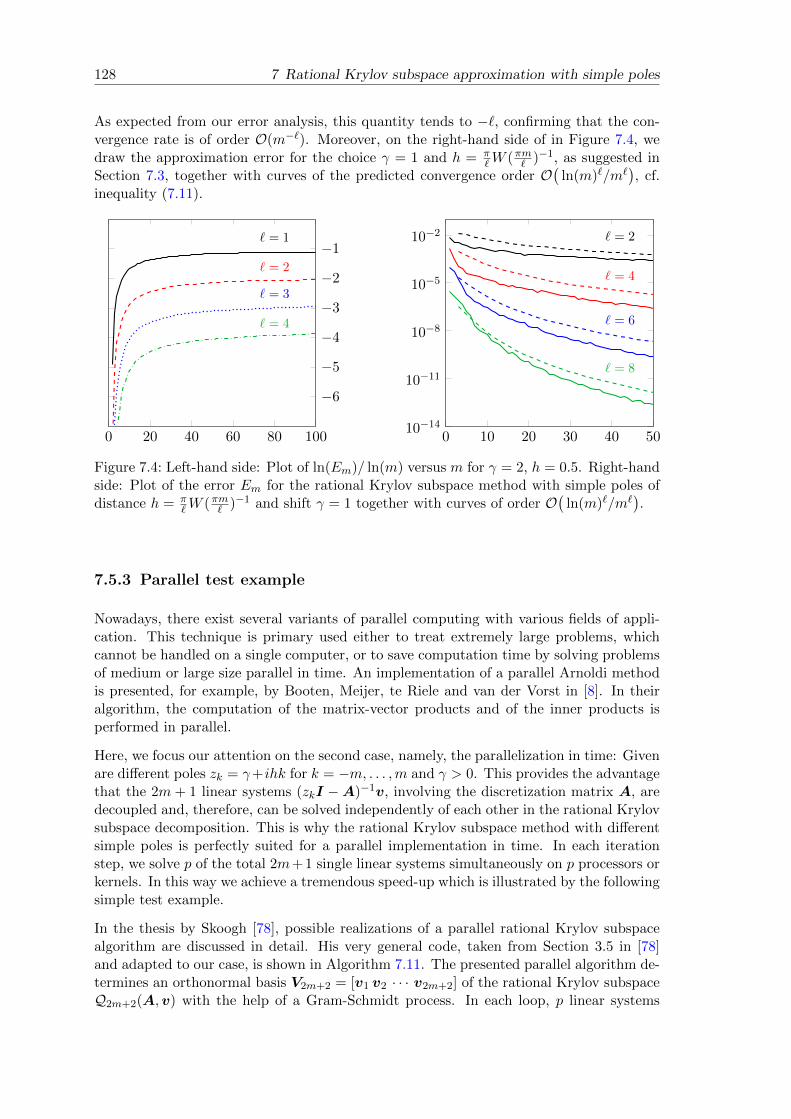
128 7 Rational Krylov subspace approximation with simple poles
As expected from our error analysis, this quantity tends to −`, confirming that the con-vergence rate is of order O(m−`). Moreover, on the right-hand side of in Figure 7.4, wedraw the approximation error for the choice γ = 1 and h = π
`W (πm` )−1, as suggested inSection 7.3, together with curves of the predicted convergence order O
(ln(m)`/m`
), cf.
inequality (7.11).
0 20 40 60 80 100
−6
−5
−4
−3
−2
−1` = 1
` = 2
` = 3
` = 4
0 10 20 30 40 5010−14
10−11
10−8
10−5
10−2 ` = 2
` = 4
` = 6
` = 8
Figure 7.4: Left-hand side: Plot of ln(Em)/ ln(m) versus m for γ = 2, h = 0.5. Right-handside: Plot of the error Em for the rational Krylov subspace method with simple poles ofdistance h = π
`W (πm` )−1 and shift γ = 1 together with curves of order O(
ln(m)`/m`).
7.5.3 Parallel test example
Nowadays, there exist several variants of parallel computing with various fields of appli-cation. This technique is primary used either to treat extremely large problems, whichcannot be handled on a single computer, or to save computation time by solving problemsof medium or large size parallel in time. An implementation of a parallel Arnoldi methodis presented, for example, by Booten, Meijer, te Riele and van der Vorst in [8]. In theiralgorithm, the computation of the matrix-vector products and of the inner products isperformed in parallel.
Here, we focus our attention on the second case, namely, the parallelization in time: Givenare different poles zk = γ+ihk for k = −m, . . . ,m and γ > 0. This provides the advantagethat the 2m + 1 linear systems (zkI −A)−1v, involving the discretization matrix A, aredecoupled and, therefore, can be solved independently of each other in the rational Krylovsubspace decomposition. This is why the rational Krylov subspace method with differentsimple poles is perfectly suited for a parallel implementation in time. In each iterationstep, we solve p of the total 2m+1 single linear systems simultaneously on p processors orkernels. In this way we achieve a tremendous speed-up which is illustrated by the followingsimple test example.
In the thesis by Skoogh [78], possible realizations of a parallel rational Krylov subspacealgorithm are discussed in detail. His very general code, taken from Section 3.5 in [78]and adapted to our case, is shown in Algorithm 7.11. The presented parallel algorithm de-termines an orthonormal basis V2m+2 = [v1 v2 · · · v2m+2] of the rational Krylov subspaceQ2m+2(A,v) with the help of a Gram-Schmidt process. In each loop, p linear systems

7.5 Numerical experiments 129
wk = (zkI −A)−1wk are solved in parallel on p different processors (or kernels) for givenstarting vectors wk. The resulting vectors wk are then orthogonalized against each otherand against all previously computed basis vectors vi. For the first iteration step withj = 1, the starting vectors wk, k = 1, . . . , p, are set to v1. In the next iterations of thewhile loop, each of the p processors can use its own orthogonalized wk of the previous step.Taking wk = vk instead, this would lead to a sequential algorithm, since the solution of(zkI −A)wk = vk is only available, if vk is known in advance. For our experiments, wesimply choose wk = v = v1 for all k.
Algorithm 7.11 Parallel rational Krylov subspace process
given: A ∈ CN×N , v ∈ CN
given: set of poles Z := zk = γ + ihk , k = −m. . . ,mv1 = v/‖v‖j = 1
while j ≤ 2m+ 1
choose vectors wk, k = 1, . . . , p
choose poles zk ∈ Z, k = 1, . . . , p
compute wk = (zkI−A)−1wk, k = 1, . . . , p (parallel step)
for k = 1, . . . , p do
for i = 1, . . . , j do
hi,j = (wk,vi)
end for
wk = wk −∑j
i=1 hi,jvi
hj+1,j = ‖wk‖vj+1 = wk/hj+1,j
j = j + 1
end for
end while
Skoogh discusses several implementations of the parallel rational Krylov subspace algo-rithm. On the one hand, one can use an additional processor, also called master, thatperforms the orthogonalization of the computed vectors wk. On the other hand, it isalso possible that each of the p so-called slave processors orthogonalizes its own computedvector. However, this requires the exchange of the orthogonalized vectors between theprocessors. More information and further details concerning, i.a., the advantages and dis-advantages of the different implementations, especially the communication time, can befound in [78]. We will not go into any more detail here.
For our purposes, we use the first variant: A master handles the program control, managesthe communication, and performs the orthogonalization, whereas every slave processorsolves one of the occurring linear systems.

130 7 Rational Krylov subspace approximation with simple poles
In order to demonstrate that a parallel computation of the rational Krylov subspace de-composition can essentially outperform the serial implementation, we consider a dense1 500× 1 500 - matrix A with the field of values W (A) = [−1 500,−1] ⊆ C−0 on the nega-tive real axis and a random vector v of norm one. We apply a serial and a parallel versionof the rational Krylov subspace method for the approximation of ϕ1(τA)v and ϕ4(τA)vwith the parameter choice τ = 0.05, γ = 1, and h = 0.25, in accordance with Table 7.1.The comparison is shown in Figure 7.2, where the approximation error is plotted againstthe computing time in seconds. The smallest error corresponds to the dimension 100 ofthe Krylov subspace, that is, m = 49 in Q2m+2(A,v).
The parallel version has been conducted on a local cluster of 13 heterogeneous workstationcomputers using MPI and the C programming language, whereas the serial process hasbeen computed on one of these workstations. Even though the network is not a high-performance network suited for parallel computations, the parallel-in-time version of therational Krylov subspace approximation with simple poles is enormously faster and thusmore efficient for our considered test problem.
Moreover, we display in Figure 7.2 the approximation error obtained by the implicit Eulermethod applied to the system of ordinary differential equations
y′(t) = Ay(t) +t`−1
(`− 1)!v , y(0) = 0
with solution y(τ) = τ `ϕ`(τA)v. This serves as a reference for standard stiff integrators.For a reasonable comparison, the results of the implicit Euler scheme are scaled by thefactor τ−`.
0 50 100 15010−8
10−6
10−4
10−2
100
0 50 100 15010−8
10−6
10−4
10−2
100
Table 7.2: Comparison of a serial (red dashed line) with a parallel (blue solid line) imple-mentation of the rational Krylov subspace method and with the implicit Euler method(green dash-dotted line) for the approximation of ϕ1(τA)v (top) and ϕ4(τA)v (bottom),where A is a dense matrix with W (A) = [−1 500,−1]. The error is plotted versus com-puting time in seconds. The parameters are chosen as τ = 0.05, γ = 1, and h = 0.25.
We performed the same numerical experiment up to the Krylov subspace dimension 450,requiring O(1012) floating point operations, which is equivalent to about 1 Tflop. Forthe approximation of ϕ1(τA)v up to an accuracy of 1.044555 · 10−9, the parallel version

7.5 Numerical experiments 131
needed 33.53 seconds and the serial variant needed 837.6 seconds, which is approximatelyequal to 14 minutes.
Furthermore, we show in Figure 7.3 the error versus computing time for the approximationof ϕ4(A)v, where A is a dense matrix with a field of values W (A) = [−1 500 i,−i] on theimaginary axis. On the left-hand side, a local cluster of 13 heterogeneous workstations hasbeen used for the computation. On the right-hand side, we computed the approximationon a single machine with 12 true kernels. Again, the parallel implementation exhibits asignificant speed-up.
0 50 100 150 200
10−7
10−6
10−5
10−4
10−3
10−2
0 200 400 600
10−7
10−6
10−5
10−4
10−3
10−2
Table 7.3: Comparison of a serial (red dashed line) with a parallel (blue solid line) imple-mentation of the rational Krylov subspace method and with the implicit Euler method(green dash-dotted line) for the approximation of ϕ4(A)v, where A is a dense matrix withW (A) = [−1 500 i,−i], γ = 1, and h = 0.25. The error is plotted versus computing timein seconds. On the left-hand side, a local cluster of 13 heterogeneous workstations hasbeen used and, on the right-hand side, a single machine with 12 true kernels.
7.5.4 Wave equation on a non standard domain
In order to compare the shift-and-invert Krylov subspace method with the rational Krylovsubspace approximation with simple poles, we return to the wave equation in Section 6.5.2,
u′′ = ∆u− u for (x, y) ∈ Ω , t ≥ 0 ,
u(0, x, y) = u0(x, y) , u′(0, x, y) = u′0(x, y) for (x, y) ∈ Ω ,
∇nu = 0 for (x, y) ∈ ∂Ω
on L2(Ω) with homogeneous Neumann boundary conditions for the non standard spatialdomain shown in Figure 6.13 above. In Section 6.5.2, we have seen that for a finite-elementdiscretization, the semi-discrete first order formulation is given as
y′(t) =
[v(t)w(t)
]′=
[O I
M−1(S −M) O
] [v(t)w(t)
]= Ay(t) , y(0) = y0 =
[v0
w0
]with (M)ij = (φi, φj)L2(Ω), (S)ij = −(∇φi,∇φj)L2(Ω), where φk(x, y) ∈ H1(Ω) are thelinear ansatz functions of the finite-element method. As initial value, we choose the vectory0 = y1
0 from Section 6.5.2.

132 7 Rational Krylov subspace approximation with simple poles
This time, we do not approximate eτAy0, but ϕ1(τA)Ay0 in the alternative representationeτAy0 = τϕ1(τA)Ay0 +y0. We compute approximations in the rational Krylov subspaceQ2m+2(τA,Ay0) with simple poles of distance h = 1 and in the shift-and-invert Krylovsubspace K2m+2((γI − τA)−1,Ay0). In both cases, we take γ = 3. For this choice ofparameters, the fixed term in the error bound (7.4), which does not depend on m, is ofsize O(10−3).
A comparison of the two methods is shown in Figure 7.5 for two different choices of τ andnumbers of triangles of the finite-element mesh. The blue solid error curve refers to therational Krylov subspace with simple poles and the red dashed error curve to the Krylovspace with one single pole. The error ‖ϕ1(τA)Ay0 − ϕ1(τAm)Ay0‖B is plotted againstm, where Am is the restriction of A to Q2m+2(τA,Ay0) or K2m+2((γI − τA)−1,Ay0),respectively. The error is measured with respect to ‖ · ‖B, where B was given as the blockdiagonal matrix B = diag(−(S −M),M).
For the solution of the shifted linear systems((γ + ihk)2M − τ2(S −M)
)x = b, cf.
(6.10) above, we can no longer use a multigrid method with Gauss-Seidel smoother. Forcomplex shifts γ+ ihk, the matrix here is not real symmetric and positive definite like thematrix γ2M−τ2(S−M) occurring in the shift-and-invert Krylov subspace approximation.Instead of the Gauss-Seidel iteration, we apply the Quasi Minimal Residual method (cf.[22]) for the smoothing process in the multigrid method as suggested in [79], Section 5.15.
0 2 4 6 810−4
10−3
10−2
10−1
100
0 2 4 6 810−5
10−4
10−3
10−2
10−1
Figure 7.5: Plot of the error ‖ϕ1(τA)Ay0 − ϕ1(τAm)Ay0‖B versus m for the rationalKrylov subspaces Q2m+2(τA,Ay0) (blue solid line) and K2m+2((γI − τA)−1,Ay0) forτ = 0.05 and a mesh with 18 816 triangles, 10 057 nodes (left), τ = 0.01 and a mesh with301 056 triangles, 153 121 nodes (right), and parameters γ = 3, h = 1.

Chapter 8
Conclusion and outlook
The goal of this thesis was to study the convergence behavior of rational Krylov subspacemethods for the approximation of ϕ`(A)v. These ϕ-functions play a fundamental role inthe application of exponential integrators for the time integration of evolution equations.Their efficient and reliable computation is presently of great interest and a subject ofcurrent research. For large stiff matrices A, that arise from the discretization of someunbounded differential operator and have a field of values in the left complex half-plane,rational Krylov methods significantly outperform the well-established standard Krylovsubspace iteration and other standard methods for stiff problems such as the implicitEuler or the Crank-Nicolson scheme.
We have analyzed the approximation of ϕ`(A)v in a rational Krylov subspace with onesingle repeated pole γ > 0 and with equidistant simple poles γ + ihk, k = −m, . . . ,m,on the line Re(z) = γ. For stiff matrices A with W (A) ⊆ C−0 , sublinear convergencerates could be shown which do not depend on the norm of the discretization matrix A.As a consequence, it is guaranteed that these rational Krylov subspace methods convergeindependent of the refinement of the spatial mesh. In contrast, the standard Krylovsubspace approximation has error bounds that always involve ‖A‖, so that this methodis not suited for our purposes.
However, if the initial value is smooth enough, it became apparent that it is often advan-tageous to first perform some cheaper standard Krylov steps and then to continue withthe more efficient but usually more expensive rational Krylov subspace process. This hasled us to study extended Krylov subspace methods. They represent a skillful combinationof the polynomial and the rational Krylov subspace iteration which results in a fastergrid-independent convergence, provided that the vector v satisfies certain smoothnessproperties.
Since the obtained error bounds for rational and extended Krylov subspace methods holduniformly over all possible grids in space, the presented techniques constitute a promisingapproximation method for the ϕ-functions evaluated at large discretization matrices A.In order to achieve an approximation to ϕ`(A)v that is as optimal as possible, we alsodiscussed suitable choices for the shift γ and the free parameter h, which determines thedistance of the equidistant poles for the rational Krylov subspace process with differentsimple poles.
In the next step, it would be interesting to examine more precisely the influence of thesmoothness of the initial data to the rational Krylov subspace approximation. The ob-servations in our numerical experiments suggest that not only the convergence rate ofthe extended method but also the rate of the rational Krylov subspace approximation isaffected by the smoothness properties of the initial vector.

134 8 Conclusion and outlook
In the case that the field of values of the matrix A has a special geometry, that is, W (A)is, for example, a subset of the negative real line or lies in a sector in the left complexhalf-plane, better convergence rate are observed than predicted by our estimates. Thenext important step could therefore be to improve the error bounds depending on theopening angle of the sector, in which the field of values is located. Such matrices with afield of values in some sector arise from the discretization of parabolic problems involvingsectorial operators.

Bibliography
[1] N. Achyeser. Uber den Jacksonschen Approximationssatz. Communications de laSociete Mathematique de Kharkow, 8(4):3–12, 1934.
[2] A. H. Al-Mohy and N. J. Higham. Computing the action of the matrix exponential,with an application to exponential integrators. SIAM Journal on Scientific Comput-ing, 33(2):488–511, 2011.
[3] B. Beckermann and S. Guttel. Superlinear convergence of the rational Arnoldi methodfor the approximation of matrix functions. Numerische Mathematik, 121(2):205–236,2012.
[4] B. Beckermann and L. Reichel. Error estimates and evaluation of matrix functionsvia the Faber transform. SIAM Journal on Numerical Analysis, 47(5):3849–3883,2009.
[5] D. Berend and T. Tassa. Improved bounds on bell numbers and on moments of sumsof random variables. Probability and Mathematical Statistics, 30(2):185–205, 2010.
[6] L. Bergamaschi and M. Vianello. Efficient computation of the exponential operatorfor large, sparse, symmetric matrices. Numerical Linear Algebra with Applications,7(1):27–45, 2000.
[7] M. C. De Bonis, G. Mastroianni, and M. Viggiano. K-functionals, moduli of smooth-ness and weighted best approximation on the semiaxis. In Functions, series, operators(Budapest, 1999), pages 181–211. Janos Bolyai Math. Soc., Budapest, 2002.
[8] J. G. L. Booten, P. M. Meijer, H. J. J. te Riele, and H. A. van der Vorst. ParallelArnoldi method for the construction of a Krylov subspace basis: an application inmagnetohydrodynamics. In HPCN, Lecture Notes in Computer Science, pages 196–201. Springer, 1994.
[9] D. Braess. Finite Elemente: Theorie, schnelle Loser und Anwendungen in der Elas-tizitatstheorie. Springer, Berlin, 4., uberarbeitete und erweiterte Auflage, 2007.
[10] P. Brenner and V. Thomee. On rational approximations of semigroups. SIAM Journalon Numerical Analysis, 16(4):683–694, 1979.
[11] J. Certaine. The solution of ordinary differential equations with large time constants.In Mathematical methods for digital computers, pages 128–132. Wiley, New York,1960.
[12] M. Crouzeix. Numerical range and functional calculus in Hilbert space. Journal ofFunctional Analysis, 244(2):668–690, 2007.
[13] C. de la Vallee Poussin. Lecons sur l’approximation des fonctions d’une variable reelle:Professees a la Sorbonne. Collection de monographies sur la theorie des fonctions.Gauthier-Villars, Paris, 1919.

136 Bibliography
[14] R. A. DeVore and G. G. Lorentz. Constructive approximation. Die Grundlehren dermathematischen Wissenschaften in Einzeldarstellungen. Springer, Berlin, 1993.
[15] V. Druskin and L. Knizhnerman. Extended Krylov subspaces: approximation of thematrix square root and related functions. SIAM Journal on Matrix Analysis andApplications, 19(3):755–771, 1998.
[16] V. L. Druskin and L. A. Knizhnerman. Error bounds in the simple Lanczos proce-dure for computing functions of symmetric matrices and eigenvalues. ComputationalMathematics and Mathematical Physics, 31:20–30, 1991.
[17] N. Dunford and J. T. Schwartz. Linear operators, Part I. Wiley classics library. WileyInterscience Publ., Hoboken, New Jersey, 1988.
[18] H. Emamirad and A. Rougirel. A functional calculus approach for the rational approx-imation with nonuniform partitions. Discrete and Continuous Dynamical Systems,22(4):955–972, 2008.
[19] K.-J. Engel and R. Nagel. A Short Course on Operator Semigroups. Universitext.Springer, 2006.
[20] T. Ericsson and A. Ruhe. The spectral transformation Lanczos method for the numer-ical solution of large sparse generalized symmetric eigenvalue problems. Mathematicsof Computation, 35(152):1251–1268, 1980.
[21] D. J. Estep, M. G. Larson, and R. D. Williams. Estimating the error of numeri-cal solutions of systems of reaction diffusion equations. Memoirs of the AmericanMathematical Society. American Mathematical Society, Providence, R.I., 2000.
[22] R. W. Freund and N. M. Nachtigal. QMR: a quasi-minimal residual method fornon-Hermitian linear systems. Numerische Mathematik, 60(3):315–339, 1991.
[23] E. Gallopoulos and Y. Saad. Efficient solution of parabolic equations by Krylovapproximation methods. SIAM Journal on Scientific and Statistical Computing,13(5):1236–1264, 1992.
[24] T. Gockler and V. Grimm. Uniform approximation of ϕ-functions in exponentialintegrators by a rational Krylov subspace method with simple poles. To appear inSIAM Journal on Matrix Analysis and Applications, 2014.
[25] T. Gockler and V. Grimm. Convergence analysis of an extended Krylov subspacemethod for the approximation of operator functions in exponential integrators. SIAMJournal on Numerical Analysis, 51(4):2189–2213, 2013.
[26] G. H. Golub and C. F. Van Loan. Matrix computations. Johns Hopkins studies in themathematical sciences. Johns Hopkins University Pr., Baltimore, Md., 4th edition,2013.
[27] A. Greenbaum. Iterative methods for solving linear systems. Frontiers in appliedmathematics. SIAM, Philadelphia, 1997.
[28] R. E. Greene and S. G. Krantz. Function Theory of One Complex Variable. GraduateStudies in Mathematics. American Mathematical Society, 3rd edition, 2006.
[29] V. Grimm. Resolvent Krylov subspace approximation to operator functions. BITNumerical Mathematics, 52(3):639–659, 2012.

Bibliography 137
[30] S. Guttel. Rational Krylov methods for operator functions, PhD thesis, TU Berg-akademie Freiberg, Germany, 2010.
[31] S. Guttel. Rational Krylov approximation of matrix functions: Numerical methodsand optimal pole selection. GAMM Mitteilungen, 36(1):8–31, 2013.
[32] S. Guttel and L. Knizhnerman. A black-box rational Arnoldi variant for Cauchy-Stieltjes matrix functions. BIT Numerical Mathematics, 53(3):595–616, 2013.
[33] E. Hairer and G. Wanner. Solving Ordinary Differential Equations II : Stiff andDifferential-Algebraic Problems. Springer, Berlin, Heidelberg, 2nd revised edition,2010.
[34] N. Hale, N. J. Higham, and L. N. Trefethen. Computing Aα, log(A), and related ma-trix functions by contour integrals. SIAM Journal on Numerical Analysis, 46(5):2505–2523, 2008.
[35] M. Hassani. Approximation of the Lambert W Function. RGMIA Research ReportCollection, 8(4), 2005.
[36] D. J. Higham and L. N. Trefethen. Stiffness of ODEs. BIT Numerical Mathematics,33(2):285–303, 1993.
[37] N. J. Higham. The scaling and squaring method for the matrix exponential revisited.SIAM Journal on Matrix Analysis and Applications, 26(4):1179–1193, 2005.
[38] N. J. Higham. Functions of matrices: theory and computation. Society for Industrialand Applied Mathematics, Philadelphia, 2008.
[39] N. J. Higham and A. H. Al-Mohy. Computing matrix functions. Acta Numerica,19:159–208, 2010.
[40] E. Hille and R. S. Phillips. Functional analysis and semi-groups. Colloquium publi-cations. American Mathematical Society, Providence, R.I., revised edition, 1957.
[41] M. Hochbruck and C. Lubich. On Krylov subspace approximations to the matrixexponential operator. SIAM Journal on Numerical Analysis, 34(5):1911–1925, 1997.
[42] M. Hochbruck and A. Ostermann. Explicit exponential Runge-Kutta methods forsemilinear parabolic problems. SIAM Journal on Numerical Analysis, 43(3):1069–1090, 2005.
[43] M. Hochbruck and A. Ostermann. Exponential Runge-Kutta methods for parabolicproblems. Applied Numerical Mathematics, 53(2–4):323–339, 2005.
[44] M. Hochbruck and A. Ostermann. Exponential integrators. Acta Numerica, 19:209–286, 5 2010.
[45] M. Hochbruck and A. Ostermann. Exponential multistep methods of Adams-type.BIT Numerical Mathematics, 51(4):889–908, 2011.
[46] M. Hochbruck, T. Pazur, A. Schulz, E. Thawinan, and C. Wieners. Efficient timeintegration for discontinuous Galerkin approximations of linear wave equations. Toappear in Journal of Applied Mathematics and Mechanics, 2014.
[47] R. A. Horn and C. R. Johnson. Topics in matrix analysis. University Press, Cambridge[u.a.], 1st publ. edition, 1991.

138 Bibliography
[48] L. Knizhnerman and V. Simoncini. A new investigation of the extended Krylovsubspace method for matrix function evaluations. Numerical Linear Algebra withApplications, 17(4):615–638, 2010.
[49] A. N. Krylov. On the numerical solution of the equation by which, in technicalmatters, frequencies of small oscillations of material systems are determined. IZV.Akad. Nauk SSSR, 7(4):491–539, 1931. in Russian.
[50] J. D. Lawson. Generalized Runge-Kutta processes for stable systems with large Lip-schitz constants. SIAM Journal on Numerical Analysis, 4:372–380, 1967.
[51] R. J. LeVeque. Finite difference methods for ordinary and partial differential equa-tions : steady-state and time-dependent problems. Society for Industrial and AppliedMathematics, Philadelphia, 2007.
[52] L. Lopez and V. Simoncini. Analysis of projection methods for rational functionapproximation to the matrix exponential. SIAM Journal on Numerical Analysis,44(2):613–635, 2006.
[53] M. Lopez-Fernandez and C. Palencia. On the numerical inversion of the Laplacetransform of certain holomorphic mappings. Applied Numerical Mathematics, 51(2-3), 2004.
[54] G. G. Lorentz. Approximation of functions. American Mathematical Society. AMSChelsea Publishing, Providence, R.I., 1986.
[55] S. H. Lui. Numerical analysis of partial differential equations. Pure and appliedmathematics: a Wiley series of texts, monographs, and tracts. Wiley, Hoboken, NewJersey, 2011.
[56] C. R. MacCluer. Boundary Value problems and Fourier Expansions. Dover Publica-tions, Mineola, New York, revised edition, 2004.
[57] M. Miklavcic. Applied Functional Analysis and Partial Differential Equations. WorldScientific Publishing Co. Pte. Ltd., Singapore, 1998.
[58] C. Moler and C. Van Loan. Nineteen dubious ways to compute the exponential of amatrix, twenty-five years later. SIAM Review, 45(1):3–49, 2003.
[59] I. Moret. On RD-rational Krylov approximations to the core-functions of exponentialintegrators. Numerical Linear Algebra with Applications, 14(5):445–457, 2007.
[60] I. Moret and P. Novati. RD-rational approximations of the matrix exponential. BITNumerical Mathematics, 44(3):595–615, 2004.
[61] S. P. Nørsett. An A-stable modification of the Adams-Bashforth methods. In Conf.on Numerical Solution of Differential Equations (Dundee, 1969), pages 214–219.Springer, Berlin, 1969.
[62] P. Novati. Using the restricted-denominator rational Arnoldi method for exponentialintegrators. SIAM Journal on Matrix Analysis and Applications, 32(4):1537–1558,2011.
[63] B. N. Parlett. A new look at the Lanczos algorithm for solving symmetric systems oflinear equations. Linear Algebra and its Applications, 29:323–346, 1980.
[64] B. N. Parlett. The symmetric eigenvalue problem. Prentice-Hall series in computa-tional mathematics. Prentice-Hall, Englewood Cliffs, NJ, 1980.

Bibliography 139
[65] A. Pazy. Semigroups of linear operators and applications to partial differential equa-tions. Applied mathematical sciences. Springer, New York, corrected 2nd printing,1992.
[66] M. A. Pinsky. Introduction to fourier analysis and wavelets. Graduate studies inmathematics. American Mathematical Society, Providence, R.I, 2009.
[67] D. A. Pope. An exponential method of numerical integration of ordinary differentialequations. Communications of the ACM, 6:491–493, 1963.
[68] H. M. Protter and C. B. Morrey. A first course in real analysis. Undergraduate textsin mathematics. Springer, New York, 2nd edition, 1991.
[69] A. Ruhe. Rational Krylov sequence methods for eigenvalue computation. LinearAlgebra and its Applications, 58:391–405, 1984.
[70] A. Ruhe. The rational Krylov algorithm for nonsymmetric eigenvalue problems. III.Complex shifts for real matrices. BIT Numerical Mathematics, 34(1):165–176, 1994.
[71] Y. Saad. Krylov subspace methods for solving large unsymmetric linear systems.Mathematics of Computation, 37(155):105–126, 1981.
[72] Y. Saad. Analysis of some Krylov subspace approximations to the matrix exponentialoperator. SIAM Journal on Numerical Analysis, 29(1):209–228, 1992.
[73] Y. Saad. Iterative methods for sparse linear systems. SIAM, Society for Industrialand Applied Mathematics, Philadelphia, 2nd edition, 2003.
[74] M. Schechter. Principles of Functional Analysis. Graduate Studies in Mathematics.American Mathematical Society, 2nd edition, 2001.
[75] T. Schmelzer and L. N. Trefethen. Evaluating matrix functions for exponential in-tegrators via Caratheodory-Fejer approximation and contour integrals. ElectronicTransactions on Numerical Analysis, 29:1–18, 2007/08.
[76] K. Schmudgen. Unbounded self-adjoint operators on Hilbert space. Graduate texts inmathematics. Springer, Dordrecht, 2012.
[77] R. B. Sidje. Expokit: A software package for computing matrix exponentials. ACMTransactions on Mathematical Software, 24(1):130–156, 1998.
[78] D. Skoogh. An implementation of a parallel rational Krylov algorithm, PhD thesis,Goteborg University and Chalmers University of Technology, Sweden, 1996.
[79] Y. Sphira. Matrix-Based Multigrid: Theory and Applications. Numerical Methodsand Algorithms. Springer US, Boston, MA, 2nd edition, 2008.
[80] F. Stenger. Approximation via Whittaker’s cardinal function. Journal of Approxi-mation Theory, 17:222–240, 1976.
[81] D. E. Stewart and T. S. Leyk. Error estimates for Krylov subspace approximations ofmatrix exponentials. Journal of Computational and Applied Mathematics, 72(2):359–369, 1996.
[82] G. W. Stewart. Afternotes goes to graduate school: lectures on advanced numericalanalysis. SIAM, Philadelphia, 1998.
[83] L. N. Trefethen, J. A. C. Weideman, and T. Schmelzer. Talbot quadratures andrational approximations. BIT Numerical Mathematics, 46(3):653–670, 2006.

140 Bibliography
[84] J. van den Eshof and M. Hochbruck. Preconditioning Lanczos approximations to thematrix exponential. SIAM Journal on Scientific Computing, 27(4):1438–1457, 2006.
[85] H. A. van der Vorst. An iterative solution method for solving f(A)x = b, using Krylovsubspace information obtained for the symmetric positive definite matrix A. Journalof Computational and Applied Mathematics, 18(2):249–263, 1987.
[86] J. von Neumann. Eine Spektraltheorie fur allgemeine Operatoren eines unitarenRaumes. Mathematische Nachrichten 4, pages 258–281, 1951.
[87] J. L. Walsh. Interpolation and approximation by rational functions in the complexdomain. Colloquium publications. American Mathematical Society, Providence, R.I.,5th edition, 1969.


![Deflation and augmentation techniques in Krylov …introduction to Krylov subspace methods and to [74] for a recent overview on Krylov subspace methods; see also [20, 21] for an advanced](https://static.fdocuments.net/doc/165x107/5edc1784ad6a402d66669cc6/deiation-and-augmentation-techniques-in-krylov-introduction-to-krylov-subspace.jpg)


![COMPUTING APPROXIMATE (BLOCK) RATIONAL ......Krylov subspace, as we have already shown for extended Krylov subspaces in [17]. Block Krylov subspace methods are an extension of Krylov](https://static.fdocuments.net/doc/165x107/5edc1787ad6a402d66669cca/computing-approximate-block-rational-krylov-subspace-as-we-have-already.jpg)


