Rational hyperholomorphic functions in R4 · doi:10.1016/j.jfa.2004.07.012. ... 123 restricted to ....

Journal of Functional Analysis 221 (2005) 122–149

www.elsevier.com/locate/jfa

Rational hyperholomorphic functions inR4

Daniel Alpaya,∗,1, Michael Shapirob,2, Dan VolokcaDepartment of Mathematics, Ben-Gurion University of the Negev, Beer-Sheva 84105, Israel

bDepartamento de Matemáticas, E.S.F.M. del I.P.N., 07300 México, D.F., MéxicocDepartment of Mathematics, Ben-Gurion University of the Negev, Beer-Sheva 84105, Israel

Received 9 January 2004; accepted 2 July 2004Communicated by Sarason

Available online 13 October 2004

Abstract

We introduce the notion of rationality for hyperholomorphic functions (functions in the kernelof the Cauchy–Fueter operator). Following the case of one complex variable, we give threeequivalent definitions: the first in terms of Cauchy–Kovalevskaya quotients of polynomials,the second in terms of realizations and the third in terms of backward-shift invariance. Alsointroduced and studied are the counterparts of the Arveson space and Blaschke factors.© 2004 Elsevier Inc. All rights reserved.

MSC: Primary 47S10; Secondary 30G35

Keywords:Hyperholomorphic functions; Rational functions; Realization theory

1. Introduction

It is well known that functions holomorphic in a domain�⊂C are exactly theelements of the kernel of the Cauchy–Riemann differential operator

� = ��x

+ i ��y

∗ Corresponding author. Fax: +972-8-647-7648.E-mail addresses:[email protected](D. Alpay), [email protected](M. Shapiro),

[email protected](D. Volok).1 Supported by the Israel Science Foundation (Grant no. 322/00).2 Partially supported by CONACYT projects as well as by Instituto Politécnico Nacional in the framework

of COFAA and CGPI programs.

0022-1236/$ - see front matter © 2004 Elsevier Inc. All rights reserved.doi:10.1016/j.jfa.2004.07.012

http://www.elsevier.com/locate/jfa

mailto:[email protected]



D. Alpay et al. / Journal of Functional Analysis 221 (2005) 122–149 123

restricted to�. A polynomial inx andy is holomorphic if, and only if, it is a polynomialin the complex variablez = x + iy, and rational holomorphic functions are quotientsof polynomials.Holomorphic functions of one complex variable have a natural generalization to the

quaternionic setting when one replaces the Cauchy–Riemann operator by the Cauchy–Fueter operator

D = ��x0

+ e1�

�x1+ e2

��x2

+ e3�

�x3.

In this expression thexj are real variables and theej are imaginary units of theskew-fieldH of quaternions (see Section 2 below for more details). Solutions of theequationDf = 0 are called left-hyperholomorphic functions (they are also called left-hyperanalytic, or left-monogenic, or regular, functions, see[18,13,23]). Right-hyperholomorphic functions are the solutions of the equation

fD = �f�x0

+ �f�x1

e1 + �f�x2

e2 + �f�x3

e3 = 0.

When trying to generalize the notions of polynomial and rational functions to thehyperholomorphic setting, one encounters several obstructions. For instance, the quater-nionic variable

x = x0 + x1e1 + x2e2 + x3e3

is not hyperholomorphic. Moreover, the point-wise product of two hyperholomorphicfunctions is not hyperholomorphic in general and the point-wise inverse of a non-vanishing hyperholomorphic function need not be hyperholomorphic.For the polynomials these difficulties were overcome by Fueter, who introduced in

[16] the symmetrized multi-powers of the three elementary functions

�1(x) = x1 − e1x0, �2(x) = x2 − e2x0, and �3(x) = x3 − e3x0.

The polynomials thus obtained are known today as the Fueter polynomials. They are(both right and left) hyperholomorphic and appear in power series expansions of hy-perholomorphic functions. In particular, a hyperholomorphic polynomial is a linearcombination of the Fueter polynomials.In this paper we introduce the notion of rational hyperholomorphic function. We

obtain three equivalent characterizations: the first one in terms of quotients and productsof polynomials, the second one in terms of realization and the last one in terms ofbackward-shift-invariance. These various notions need to be suitably defined in thehyperholomorphic setting. A key tool here is the Cauchy–Kovalevskaya product ofhyperholomorphic functions.

124 D. Alpay et al. / Journal of Functional Analysis 221 (2005) 122–149

We also introduce a reproducing kernel Hilbert space of left-hyperholomorphic func-tions which seems to be the counterpart of the Arveson space of the ball—the repro-ducing kernel Hilbert space of functions holomorphic in the open unit ball ofCN withthe rational reproducing kernel 1

1−∑ zjwj. WhenN = 1, this is just the Hardy space

of the open unit disk. It was first introduced by Drury in[14] and proved in recentyears to be a better extension of the Hardy space than the classical Hardy space of theunit ball of CN , at least for problems in operator theory (see for instance the papers[1,2,9,10,12]for a sample of examples and applications). In particular, it is invariantunder the operatorsMzj of multiplication by the variableszj , j=1, . . . , N , and it holdsthat

I −N∑1

MzjM∗zj

= C∗C, (1.1)

whereC is the point evaluation at the origin.To explain our approach let us consider briefly first the case of holomorphic functions

of one complex variable. Letf andg be two functions holomorphic in a neighborhoodof the origin, with the power series expansions

f (z) =∞∑n=0

znan and g(z) =∞∑n=0

znbn (1.2)

at the origin. Then the point-wise product(fg)(z) = f (z)g(z) has at the origin theexpansion

(fg)(z) =∞∑n=0

zncn, (1.3)

where the sequence{cn}, given by

cn =n∑m=0

ambn−m, (1.4)

is called the convolution of the sequences{an} and{bn}. It appears that the substitute forpoint-wise product in the hyperholomorphic setting (the Cauchy–Kovalevskaya product)is also a convolution.In the 1960s, the state space theory of linear systems gave rise to a representation

of a rational function calledrealization (see [20,11]). Still assuming analyticity in aneighborhood of the origin, this representation is of the form

r(z) = D + zC(I − zA)−1B, (1.5)


whereA,B,C,D are matrices of appropriate dimensions. It is particularly suitable forthe study of matrix-valued rational functions.Realization theory has various extensions in the setting of several complex variables;

see e.g.[17,28]. One approach, related to functions holomorphic in the unit ball, ex-ploits the so-called Gleason problem (see[4,3]). A solution of the Gleason problem,due to Leibenson (see[19], [26, Section 15.8, p. 151]), was adapted to the settingof hyperholomorphic functions in[8] and [7]. It leads naturally to the analogues of(1.2)–(1.4); these are the expansions in terms of Fueter polynomials and the Cauchy–Kovalevskaya product, mentioned above. Moreover, in this way we obtain the analogueof the realization (1.5) and other equivalent descriptions of the class of rational hy-perholomorphic functions, as well as the reproducing kernel of the counterpart of theArveson space (quite different from the quaternionic Cauchy kernel).This paper is organized as follows. In Section 2 we review facts from the quaternionic

analysis and present some preliminary results, concerning backward-shift operators inthe hyperholomorphic setting. In Section3 we give three definitions of a rationalfunction in the hyperholomorphic case and prove their equivalence. In Section4 wedefine and study the counterparts of the Arveson space of the unit ball and the Blaschkefactors.Some of the results presented here were announced in[5]. In forthcoming papers

we will consider the theory of linear systems in the quaternionic case and Beurling-Lax-type theorems for the Arveson space in the present setting.

2. Quaternions and hyperholomorphic functions

2.1. The skew-field of quaternions

In this section, we provide some background on quaternionic analysis needed in thispaper. For more information, we refer the reader to[27] and to [6]. The Hamiltonskew-field of quaternionsH is the real four-dimensional linear spaceR4 equipped withthe product, defined as follows.For the elements of the standard basise0,e1,e2,e3 the rules of multiplication form

the Cayley table:

e0 e1 e2 e3e0 e0 e1 e2 e3e1 e1 −e0 e3 −e2e2 e2 −e3 −e0 e1e3 e3 e2 −e1 −e0

(2.1)


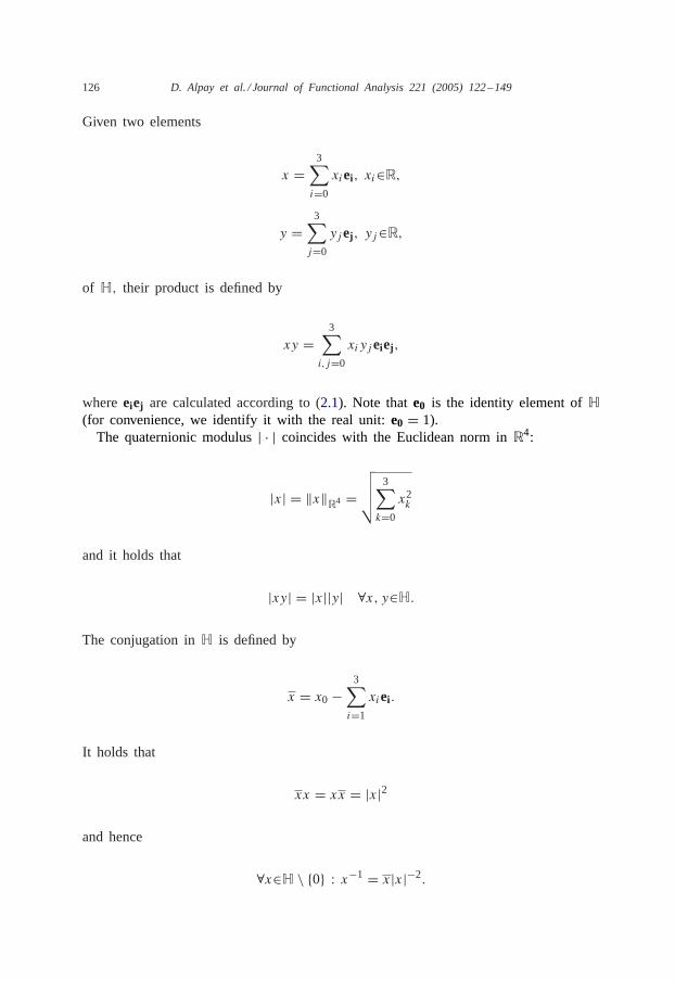
Given two elements

x =3∑i=0xiei, xi∈R,

y =3∑j=0

yjej , yj∈R,

of H, their product is defined by

xy =3∑

i,j=0xiyjeiej ,

whereeiej are calculated according to (2.1). Note thate0 is the identity element ofH(for convenience, we identify it with the real unit:e0 = 1).The quaternionic modulus| · | coincides with the Euclidean norm inR4:

|x| = ‖x‖R4 =√√√√ 3∑k=0x2k

and it holds that

|xy| = |x||y| ∀x, y∈H.

The conjugation inH is defined by

x = x0 −3∑i=1xiei .

It holds that

xx = xx = |x|2

and hence

∀x∈H \ {0} : x−1 = x|x|−2.


2.2. Hyperholomorphic functions and the Cauchy–Kovalevskaya product

We have already mentioned in Section1 that anH-valued functionf, R-differentiablein an open connected set�⊂H, is said to be left-hyperholomorphic in� if it satisfiesin � the following differential equation:

3∑i=0

ei�f�xi

= 0. (2.2)

Analogously, anH-valued functionf, R-differentiable in an open connected set�⊂H,

is said to be right-hyperholomorphic in� if it satisfies in� the differential equation

3∑i=0

�f�xi

ei = 0. (2.3)

The differential operator

D =3∑i=0

ei�

�xi

is called the Cauchy–Fueter operator. It satisfies the identity

DD = DD = �4,

where

D = ��x0

−3∑j=1

ej�

�xjand �4 =

3∑i=0

�2

�x2i.

Thus hyperholomorphic functions are, in particular, harmonic.In the sequel we shall restrict ourselves to the case of left-hyperholomorphic func-

tions. One can, of course, obtain analogous results for right-hyperholomorphic functions,as well.Let us denote the right-H-module of functions, left-hyperholomorphic in�, by

OH(�). Assume that� is a ball, centered at the origin. Then, as was proved in[7], any elementf∈OH(�) can be written in the form

f (x) = f (0)+3∑n=1

�n(x)Rnf (x), (2.4)


where

�n(x) = xn − x0en (2.5)

are entire (both right and left) hyperholomorphic functions, and the operators

Rn : OH(�) �→ OH(�)

are defined by

Rnf (x) =1∫0

�f�xn

(tx) dt. (2.6)

(see [24, p. 118; 26, Section 15; 8, p. 151; 3]for these operators in the setting ofthe unit ball ofCN ). Note that it follows from the hyperholomorphic Cauchy integralformula thatOH(�)⊂C∞(�), hence the operatorsRn commute:

RmRnf (x) =1∫0

1∫0

�2f�xn�xm

(utx)t dt du = RnRmf (x)

and that

Rnf (0) = �f�xn

(0).

Hence, applying the formula (2.4) for Rnf , we get

f (x) = f (0)+3∑n=1

�n(x)�f�xn

(0)+∑

0�n�m�3

(�n(x)�m(x)+ �m(x)�n(x)

)RmRnf (x).

Iterating this process, one obtains an expansion off in terms of symmetrized productsof �n, analogous to the classical Taylor power series expansion.To be more precise, let us introduce the multi-index notation we shall use throughout

this paper. The symmetrized product ofa1, . . . , an∈H is defined by

a1 × a2 × · · · × an = 1

n!∑�∈Sn

a�(1)a�(2) · · · a�(n),


whereSn is the set of all permutations of the set{1, . . . , n}. Furthermore, for�,�∈Z3+we use the usual notation

|�| = �1 + �2 + �3, �! = �1!�2!�3!, �� if �j��j ∀j,

�� = �|�|

�x�11 �x�2

2 �x�33

,

e1 = (1 0 0

), e2 = (

0 1 0), e3 = (

0 0 1).

Using the above notation, we can formally write

f (x) =∞∑n=0

∑|�|=n

��(x)f�, (2.7)

where

��(x)= �1(x)×�1 × �2(x)

×�2 × �3(x)×�3, (2.8)

f�= 1

�! (��f )(0). (2.9)

The polynomials��, defined by (2.8), are called the Fueter polynomials. It can beproved that the Fueter polynomials are entire (both left and right) hyperholomorphicand that the series (2.7) is normally convergent. Thus one can characterize the right-H-moduleOH of functions, left-hyperholomorphic in a neighborhood of the origin, asfollows (see[13]):

Theorem 2.1. An H-valued functionf, defined in a neighborhood of the origin, be-longs to the spaceOH if, and only if, it can be represented in the form(2.7),where

�(f ) = lim supn→∞

∑

|�|=n|f�|

1n

<∞. (2.10)

In this case the series(2.7) converges uniformly on compact subsets of the ball

{x∈H : |x| · �(f ) < 1}.


Corollary 2.2. An H-valued polynomial p of real variablesx0, x1, x2, x3 is left-hyperholomorphic if, and only if, it is a finite linear combination of Fueter polynomials:

p(x) =m∑n=0

∑|�|=n

��p�, p�∈H.

Remark 2.3. In view of Theorem2.1, in the quaternionic analysis the elementaryfunctions�n play role, similar in a sense to that ofzn in several complex variables. Thus�n are sometimes called the hyperholomorphic variables. The term “total variables" isused also referring to the fact that both�n and all its powers are hyperholomorphic, see[13,18]. We note, however, that�n are neither independent, norH-linear. Moreover, thechoice of left-hyperholomorphic variables is not unique: e.g.,�n(e1x) are also suitablefor this role, but are not right-hyperholomorphic.

It is useful to calculate the expressions for the operatorsRn, defined by (2.6), interms of expansions (2.7).

Lemma 2.4. Let f∈OH(�) be given by(2.7). Then

Rnf (x) =∑��en

�n|�|�

�−en(x)f�. (2.11)

Proof. Without loss of generality,f is a Fueter polynomial. But

��

�xn(x) = �n�

�−en(x),

hence

Rn��(x)=

1∫0

��

�xn(tx) dt

=1∫0

�nt |�|−1��−en(x) dt = �n|�|�

�−en(x). �

In view of Lemma2.4, we propose the following

Definition 2.5. The operatorsRn:OH �→OH, defined by (2.11), are called the backward-shift operators.


Following the analogy with the complex case, we would like to impose onOH thestructure of a ring. However, the point-wise product is not suitable here. For instance,the function�1�2 is not hyperholomorphic. Instead, one can use (see[13, Section 14]and compare with (1.2)–(1.4) in Section1) the following

Definition 2.6. The Cauchy–Kovalevskaya product (below: C–K-product)f�g of thefunctions

f =∑

��f�, g =∑

��g�,

left-hyperholomorphic in a neighborhood of the origin, is defined by

f � g =∞∑n=0

∑|�|=n

��∑

0��

f�g�−�. (2.12)

Remark 2.7. Note that

(f � g) ∣∣x0=0= f

∣∣x0=0 · g ∣∣

x0=0

and hence the C–K-product is the Cauchy–Kovalevskaya extension (see for instance[21, Section 1.7]) with respect to the Cauchy–Fueter operator of the point-wise productin R3. This explains the terminology.

Remark 2.8. In certain special cases the C–K-product coincides with the point-wiseone. For instance, ifg(x) ≡ const thenf�g = fg, but not necessarilyg�f = gf !Another special case is discussed in Section3.4.

Proposition 2.9. The spaceOH, equipped with the C–K-product, is a ring. Moreover,

�(f�g)� max{�(f ),�(g)}.

Proof.Without loss of generality, we take�(f ) = �(g) = �. Then∀>0, ∃C()>0,∀k :∑|�|=k

|a�|�C()(� + )k,

∑|�|=k

|b�|�C()(� + )k.


Hence

∑|�|=n

|∑

0��

a�b�−�|�∑|�|=n

∑0��

|a�||b�−�|�n∑k=0

∑|�|=k

|a�|∑

|�|=n−k|b�|

�(n+ 1)C()2(� + )n

and so

�(f�g)��. �

The C–K-product can be generalized to spaces of matrix-valued left-hyperholo-morphic functions in the usual way: for

F = (f,�)∈Om×nH , G = (g�,�)∈On×pH

we define

F�G =∑

�

f,��g�,�

,�

.

The question arises, when an elementF∈On×nH is C–K-invertible. In view of (2.12), anecessary condition is that the valueF(0) must be invertible inHn×n. This turns outto be also sufficient:

Proposition 2.10. Let F∈On×nH . If F(0) is invertible in H then F is C–K-invertible inOn×nH and its C–K-inverseF−�∈On×nH is given by the series

F−� = (F (0))−1�(In −G)−� = (F (0))−1�∞∑k=0G�k, (2.13)

where

G = In − F(F(0))−1.

Proof. It suffices to show the normal convergence of the series

(In −G)−� =∞∑k=0G�k (2.14)


in a neighborhood of the origin for arbitraryG∈On×nH , satisfyingG(0) = 0. Accordingto Theorem2.1,

G =∞∑p=1

∑|�|=p

��A�

and there existsA∈R+ such that

∀p > 0:∑|�|=p

‖A�‖�Ap,

where‖ · ‖ denotes the operator norm. Then

G�k =∞∑p=k

∑|�|=p

��∑

�1 + . . .+ �k = ��1, . . . ,�k �= 0

A�1 · · ·A�k .

But for p�k�1∑|�|=p

‖∑

�1 + . . .+ �k = ��1, . . . ,�k �= 0

A�1 · · ·A�k‖

�∑

p1 + . . .+ pk = pp1, . . . , pk > 0

∑|�1|=p1

‖A�1‖ · · ·∑

|�k |=pk‖A�k‖

�(p − 1k − 1

)Ap < (2A)p.

Therefore,

|x| < 1

4A⇒‖G�k(x)‖� 1

2k−1,

and the normal convergence of the series (2.14) in the ball{x:|x|<1/4A} follows. �

2.3. The Gleason problem in the hyperholomorphic case

In view of Remark 2.3, the formula (2.4) may be considered as a solution fora Gleason problem with respect to the hyperholomorphic variables�n (see [8,7] for


details and references). However, there is a disadvantage in that the point-wise prod-uct appears. In particular, the individual terms�n(x)Rnf (x) in the sum (2.4) neednot be left-hyperholomorphic, in general. The goal of the present section is to con-sider the Gleason problem with the point-wise product being replaced by the C–K-product.

Definition 2.11. Let f∈OH. The Gleason problem forf is to find a triple of functionsg1, g2, g3∈OH, such that

f − f (0) =3∑n=1

�n�gn.

It turns out that the backward-shift operatorsRn provide a solution for this newGleason problem, as well.

Theorem 2.12.Let f∈OH. Then it holds that

f − f (0) =3∑n=1

�n�Rnf. (2.15)

Proof. According to (2.11), we have

3∑n=1

�n�Rnf =3∑n=1

∑��en

�n|�|�

�f� =∑|�|>0

��f� = f − f (0). �

In general, the solution for the Gleason problem, provided by the backward-shiftoperators, is not the only possible one. To illustrate this observation, let us considerthe subspaces ofOmH, in which the problem is solvable.

Definition 2.13. A subspaceW of OmH is said to be resolvent-invariant if

∀f∈W ∃g1, g2, g3∈W : f − f (0) =3∑n=1

�n�gn.

If, moreover, the spaceW is Rn-invariant forn = 1,2,3 then it is said to be backward-shift-invariant.

Theorem 2.14.A finite-dimensional subspaceW of OmH is resolvent-invariant(respec-tively, backward-shift-invariant) if, and only if, it is spanned by the columns of a


matrix-valued function of the form

W = C�(I −

3∑n=1

�nAn

)−�, (2.16)

where C andAn are constant matrices with entries inH (respectively, An commute).

In the proof of Theorem2.14 we shall use the following.

Lemma 2.15. Let A1, A2 and A3 be in H'×'. Then in a neighborhood of the originit holds that

(I' − �1A1 − �2A2 − �3A3)−� =

∑�∈Z3+

��A� |�|!�! , (2.17)

where

A� = A×�11 × A×�2

2 × A×�33 . (2.18)

Proof. We have

(I' − �1A1 − �2A2 − �3A3)−� =

∞∑k=0

(�1A1 + �2A2 + �3A3

)�k.

Let us prove by induction onk that

(�1A1 + �2A2 + �3A3

)�k =∑|�|=k

��(A

×�11 × A×�2

2 × A×�33

) |�|!�! . (2.19)

Indeed, (2.19) obviously holds fork = 0, and if it holds for somek then we have

(�1A1 + �2A2 + �3A3

)�(k+1)=(�1A1 + �2A2 + �3A3)� ∑

|�|=k��A� |�|!

�!

=∑

|�|=k+1�� (|�| − 1)!

�!

×(�1A1A�−e1 + �2A2A�−e2 + �3A3A�−e3)=

∑|�|=k+1

��A� |�|!�! . �


Proof of Theorem 2.14.Let W be a resolvent-invariant finite-dimensional subspaceof OmH and letW be a matrix-valued hyperholomorphic function whose columns forma basis ofW. Then there exist constant matricesAn∈H'×' (with ' = dimW) andC = W(0), such that

W = C +3∑n=1

�n�WAn = C +W�3∑n=1

�nAn,

henceW is of the form (2.16). If W is, moreover, backward-shift-invariant thenAncan be chosen to satisfyRnW = WAn. Since the operatorsRn commute, the matricesAn chosen in this way commute, as well.Conversely, letW be the span of the columns of a matrix-valued function of the

form (2.16). Then

W −W(0)=C�(I −

3∑n=1

�nAn

)−�− C

=W�(I −

(I −

3∑n=1

�nAn

))=

3∑n=1

�n�WAn

and henceW is resolvent-invariant. If, moreover, the matricesAn commute then,

according to Lemma2.15,

W =∑�∈Z3+

��CA�11 A

�22 A

�33

|�|!�! ,

henceRnW = WAn. This completes the proof.

3. Rational hyperholomorphic functions

3.1. Definitions

In this section we give three definitions of a rational function, left-hyperholomorphicin a neighborhood of the origin. We prove that they are equivalent in Section3.3.The first definition parallels the classical definition in terms of quotients of polyno-

mials in the complex case. Here polynomials are replaced by the Fueter polynomials,point-wise multiplication is replaced by the C–K-product, and inverses are replaced bythe C–K-inverses.


Definition 3.1. An Hm×n-valued functionR, left-hyperholomorphic in a neighborhoodof the origin, is said to be rational if all its entries belong to the minimal subringQH ofOH, which contains hyperholomorphic polynomials and is closed under C–K-inversion:

r∈QH, r(0) �= 0⇒∃r−�∈QH.

Example 3.2. Let j = 1,2,3. The functions�j , �2j and more generally all the Fueterpolynomials are rational.

Example 3.3. The function

(((1− �1e1)

−� + 2)−� + �1��3

2

)−� + ��53 e3

is rational.

The next example will play an important role in the sequel.

Example 3.4. Let a∈H. The function

x �→(1− �1�1(a)− �2�2(a)− �3�3(a))−� (3.1)

is rational.

Remark 3.5. Note that Definition3.1, admits the following interpretation in terms ofthe Cauchy–Kovalevskaya extension (see Remark2.7): an Hm×n-valued functionR,left-hyperholomorphic in a neighborhood of the origin, is rational if and only if itsrestriction to the hyperplanex0 = 0 is of the form

R∣∣x0=0=

Q(x1, x2, x3)

r(x1, x2, x3),

whereQ is anHm×n-valued polynomial andr is anR-valued polynomial,r(0) �= 0.Hence, for instance, the quaternionic Cauchy kernel

E(y − x) = 1

vol S3y − x

|y − x|4 ,

considered for a fixedy �= 0 as a hyperholomorphic function in{x:|x|<|y|}, isrational.We would like to mention also that in the special case whenR

∣∣x0=0 is a real-

valued rational function which can be, moreover, decomposed into the product of


complex-valued rational functions of degree one, an explicit integral representation forthe rational hyperholomorphic functionR(x) was obtained by Laville in[22].

The second definition parallels the realization (1.5) (see Section1) in the complexcase.

Definition 3.6. An Hm×n-valued functionR, left-hyperholomorphic in a neighborhoodof the origin, is said to be rational if it can be represented in the form

R = D + C�(I − �1A1 − �2A2 − �3A3)−��(�1B1 + �2B2 + �3B3), (3.2)

where Ai, Bi , C and D are constant matrices with entries inH and of appropriatedimensions.

For brevity, from now on we shall use the notation

�(') = (�1I' �2I' �3I'

)∈O'×3'H . (3.3)

The dimension' will usually be understood from the context and will be omitted. Then(3.2) can be rewritten as:

R = D + C�(I − �A)−��B, (3.4)

where

A =A1A2A3

and B =

B1B2B3

. (3.5)

The third definition is in terms of the resolvent-invariance.

Definition 3.7. An Hm×n-valued functionR, left-hyperholomorphic in a neighborhoodof the origin, is said to be rational if there is a finite-dimensional resolvent-invariantspaceW⊂OmH, such that for everyv∈Hn the Gleason problem forRv is solvablein W.

The main result of the paper, presented in Section3.3, is that all three definitionsare equivalent. In view of Proposition2.15, they are also equivalent to the following.

Definition 3.8. An Hm×n-valued functionR, left-hyperholomorphic in a neighborhoodof the origin, is said to be rational if it can be represented as

R =∞∑n=0

∑|�|=n

��R�,


where for |�|�1

R� = (|�| − 1)!�! C

(�1A�−e1 �2A�−e2 �3A�−e3 )B

with A,B,C being constant matrices of appropriate dimensions.

3.2. Preparatory lemmas

The proof of the equivalence of Definitions3.1–3.7 is based on several technicallemmas.

Lemma 3.9. Let R∈On×nH admit the representation(3.4), whereD∈Hn×n is invertible.Then R is C–K-invertible and its C–K-inverseR−� admits the representation

R−� = D−1 −D−1C�(I − ZA)−��ZBD−1, (3.6)

where A = A− BD−1C.

Proof. We have:

(D + C�(I − �A)−��B)�(D−1 −D−1C�(I − �A)−��BD−1)

= I − C�(I − �A)−��BD−1 + C�(I − �A)−��BD−1

−C�(I − �A)−��BD−1C�(I − �A)−��BD−1

= I − C�{(I − �A)−� − (I − �A)−�

+(I − �A)−��BD−1C�(I − �A)−�}��BD−1.

But

�BD−1C = �(A− A) = (I − �A)− (I − �A),

hence the expression in the curly brackets is equal to 0. �

Lemma 3.10. There exists a unitary matrixU∈H3('+m)×3('+m) such that

diag (�('), �(m)) = �('+m)U. (3.7)


Proof. It suffices to take

U =

I' 0 0 0 0 00 0 0 Im 0 00 I' 0 0 0 00 0 0 0 Im 00 0 I' 0 0 00 0 0 0 0 Im

. �

Lemma 3.11. Let Ri∈Omi×niH , i = 1,2, admit the representations

Ri(x) = D(i) + C(i)�(I − �A(i))−��B(i).

If n2 = m1 thenR1�R2 admits the representation

R1�R2=D(1)D(2)

+ (C(1) D(1)C(2) )�(I − �U

(A(1) B(1)C(2)

0 A(2)

))−��U

(B(1)D(2)

B(2)

).

If m1 = m2, n1 = n2 thenR1 + R2 admits the representation

R1 + R2=D(1) +D(2)

+ (C(1) C(2) )�(I − �U

(A(1) 00 A(2)

))−��U

(B(1)

B(2)

).

In both formulas U is as in Lemma 3.10.

Proof. We have:

R1�R2=D(1)D(2) +D(1)C(2)�(I − �A(2))−��B(2)

+C(1)�(I − �A(1))−��B(1)D(2)

+C(1)�(I − �A(1))−� � �B(1)C(2)�(I − �A(2))−� � �B(2)

=D(1)D(2) + (C(1) D(1)C(2)

)�(−� −−��−�0 �−�

)�(

�B(1)D(2)

�B(2)

),


where

=I − �A(1),

�=−�B(1)C(2),

�=I − �A(2).

Using the formula

(−� −−��−�0 �−�

)=(

�0 �

)−�,

we have:

R1�R2=D(1)D(2)

+ (C(1) D(1)C(2) )�( I − �A(1) −�B(1)C(2)

0 I − �A(2)

)−��(

�B(1)D(2)

�B(2)

)

=D(1)D(2)

+ (C(1) D(1)C(2) )�(I − �U

(A(1) B(1)C(2)

0 A(2)

))−��U

(B(1)D(2)

B(2)

).

In order to obtain the second formula, it is enough to apply the first one for

(R1 I

)�(I

R2

). �

3.3. Equivalence between the various definitions

Proposition 3.12. Definitions3.7 and 3.6 are equivalent.

Proof. Indeed, ifR∈Om×nH admits the representation (3.4), whereAi∈Hp×p, let us

denote byW the span of columns of the matrix-functionW = C�(I − �A)−�. Ac-cording to Theorem2.14, the finite-dimensional spaceW is resolvent-invariant, and∀v∈Hn the functions

Gk = C�(I − �A)−�Bkv∈W, k = 1,2,3,

are a solution of the Gleason problem forRv.Conversely, assume thatW⊂OmH is a finite-dimensional resolvent-invariant space, in

which ∀v∈Hn the Gleason problem forRv is solvable. According to Theorem2.14,


there exists a matrix-function of the formW = C�(I − �A)−�, whose columns spanW. Hence there exist constant matricesBk such that

R − R(0) =3∑k=1

�k�WBk.

Since the hyperholomorphic variables (and, more generally, all the Fueter polynomials)belong to the center of the ringOH, we obtain forR the representation (3.2) withD = R(0). �

Proposition 3.13. Definitions3.1 and 3.6 are equivalent.

Proof. First of all we note that, in view of Lemmas3.9 and3.11, the space of elementsof OH which admit the representation (3.2) is a subring, which is closed under theC–K-inversion. Substituting in (3.2) Bk = 0 (respectively,C = Bk = 1, D = Ak = 0),we see that this subring contains constant functions (respectively, hyperholomorphicvariables), hence it also containsQH. In other words, every function, rational in thesense of Definition3.1, admits the representation (3.2).In order to prove the converse implication, it suffices to show that every entry of

(I −

3∑k=1

�kAk

)−�

belongs toQH. We proceed by induction on dimAk. Denote

Ak =(Ak ak

ak Ak

).

Then

I −3∑k=1

�kAk =(

��

),

where

= I −3∑k=1

�kAk, � = −3∑k=1

�kak,

� = −3∑k=1

�kak, = I −3∑k=1

�kAk.


Furthermore,

(I −

3∑k=1

�kAk

)−�

=( (

)−� − ()−� �� −�

− −�� ()−� −� + −�� (

)−� �� −�

),

where

= − �� −��.

By definition and the induction assumption, all the entries of()−�

,�, �, −� belongto QH. �

3.4. Rational functions of two complex variables

Writing

x = z1 + z2e2, where z1 = x0 + x1e1, z2 = x2 + x3e1,

one can identify the skew field of quaternionsH with the two-dimensional complexspaceC2, endowed with the special structure where, in particular,

ze2 = e2z.

The complex variablesz1 and z2 have the following properties:z1 is (both right andleft) hyperholomorphic,z2 is right-hyperholomorphic,z2 is left-hyperholomorphic. Itholds that

z1(x) = �1(x)e1, z2(x) = �2(x)− �3(x)e1, x∈R4.

Moreover, it follows from (2.9) that

zm1 z2n = z�m1 �z2�n.

From here we conclude that complex-valued functions of two complex variablesz1 andz2, holomorphic in a neighborhood of the origin, are also left-hyperholomorphic, forwhich the C–K-product and the point-wise product coincide. It follows that rationalfunctions ofz1 and z2, holomorphic in a neighborhood of the origin, are also rationalin the sense of our Definitions3.1–3.7.


4. Quaternionic Arveson space

4.1. Positive rational kernel

In this section we define and study what we believe to be the appropriate coun-terpart of the Arveson space of the unit ball (see Section1) in the setting of left-hyperholomorphic functions.To begin with, let us recall Definition2.5 of the backward-shift operatorsRn and

formulate the following.

Proposition 4.1. The common eigenvectors of the backward-shift operatorsR1, R2,R3 are functions of the form

(1− �a)−�,

wherea∈H3.

Proof. This is a special case of Theorem2.14: we are looking for 1-dimensionalbackward-shift-invariant spaces.�Set

�={x∈H : 3x20 + x21 + x22 + x23 < 1

}, (4.1)

ky(x)=(1− ��(y)∗)−�(x), y∈�. (4.2)

According to Definition3.1, the left-hyperholomorphic functionky is rational. In viewof Lemma2.15, we have

ky(x) =∑�∈Z3+

|�|!�! ��(x)��(y). (4.3)

The functionky is therefore positive in� and there exists an associated right-linearreproducing kernel Hilbert space which is an extension of the classical Hardy space;see[6]. As a direct consequence of the power expansion (4.3) we obtain:

Theorem 4.2. The reproducing kernel right-linear Hilbert spaceH(k) with reproducingkernel ky (we shall call this space the(left) quaternionic Arveson space) is the set offunctions of the form(2.7) endowed with theH-valued inner product

〈f, g〉 =∑�∈Z3+

�!|�|!g�f�. (4.4)


Remark 4.3. We note that�� and�� are orthogonal in the Arveson space when� �= �.In the quaternionic Hardy space this orthogonality condition holds only when moreover|�| �= |�|.

Let us consider the C–K-multiplication operators

M�nf = �n�f, n = 1,2,3. (4.5)

Proposition 4.4. For n = 1,2,3 the operatorM�n is a contraction from the spaceH(k) into itself.

Proof. For f∈H(k) we have

〈M�nf,M�nf 〉=∑�∈Z3+

(� + en)!|� + en|! |f�|2 =

∑�∈Z3+

�n + 1

|�| + 1

�!|�|! |f�|2

�∑�∈Z3+

�!|�|! |f�|2 = 〈f, f 〉. �

Proposition4.4 implies, in particular, that the C–K-multiplication operatorM�n isa bounded linear operator fromH(k) into itself, hence, according to the quaternionicversion of the Riesz theorem (see[13] and [25] for more details on quaternionicHilbert spaces and quaternionic adjoint operators ), it has the Hilbert adjointM∗

�n:

H(k)�→H(k), defined by

〈M�nf, g〉 = 〈f,M∗�ng〉 ∀f, g∈H(k).

The latter turns out to coincide with the backward-shift operatorRn:

Proposition 4.5.

M∗�n

= Rn|H(k).

Proof. We have∀�∈Z3+, ∀��en:

〈Rn��, ��〉 =

⟨�n|�|�

�−en , ��⟩

= (� + en)!|� + en|!

�−en� = 〈��, ��+en〉 = 〈��,M�n�

�〉.

Analogously, if�n = 0 then

〈Rn��, ��〉 = 0= 〈��, ��+en〉 = 〈��,M�n�

�〉. �


Let us denote byC : H(k)�→H the operator of evaluation at the origin:Cf=f (0).Then, in view of Proposition4.5 and Theorem2.12 for the C–K-multiplication operatorM� : H(k)3 �→H(k) the following operator identity holds true

I − M�M∗� = C∗C. (4.6)

The identity (4.6) is the quaternionic counterpart of (1.1). In the next section weshall use it to obtain the counterpart of the Blaschke factors in the quaternionic Arvesonspace.

4.2. Blaschke factors

Definition 4.6. Let a∈�. We define the Blaschke factorBa∈H(k)1×3 by

Ba = (1− �(a)�(a)∗)12 (1− ��(a)∗)−�� (

� − �(a)) (I − �(a)∗�(a)

)− 12 . (4.7)

Theorem 4.7. The C–K-multiplication operator

Ba = MBa : H(k)3 �→H(k)

is a contraction, and the following operator identity holds:

I − BaB∗a = (1− �(a)∗�(a))

(I − M�M∗

�(a)

)−1 C∗C(I − M�M∗

�(a)

)−∗. (4.8)

Proof. The proof follows the arguments of[4]. We first note that the operators

I − M�(a)M∗�(a) and I − M∗

�(a)M�(a)

are self-adjoint and strictly contractive and hence the operators

(I − M�(a)M∗

�(a)

)±1/2and

(I − M∗

�(a)M�(a)

)±1/2

are well defined. We set

H :=

(I − M�(a)M∗

�(a)

)−1/2 −M�(a)

(I − M∗

�(a)M�(a)

)−1/2

−M∗�(a)

(I − M�(a)M∗

�(a)

)−1/2 (I − M∗

�(a)M�(a)

)−1/2

.

Then it holds that

HJH∗ = H∗JH = J,


where

J =(IH(k) 00 −IH(k)3

).

(H is “the Halmos extension" of−M�(a); see[15].) Thus

C∗C = I − M�M∗� = (

I M�)J

(I

M∗�

)= (

I M�)HJH∗

(I

M∗�

)= XJX ∗, (4.9)

where

X=(X1 X2),

X1=(I − M�M∗�(a))

(I − M�(a)M∗

�(a)

)−1/2,

X2=(M� − M�(a))(I − M∗

�(a)M�(a)

)−1/2.

To conclude we remark that the operatorI − M�(a)M∗�(a) is the operator of multi-

plication by the positive number 1− �(a)�(a)∗ and therefore commutes with all theother operators under consideration. Multiplying the first and the last expressions inthe equality (4.9) by

(I − M�(a)M∗

�(a)

)1/2(I − M�M∗

�(a))−1

on the left and by its adjoint on the right we obtain (4.8). �Theorem4.7 allows to get some preliminary results on interpolation in the Arveson

space. Here we have:

Theorem 4.8. Let a∈�. Then

{f∈H(k) : f (a) = 0} ⊂ranBa. (4.10)

Proof. The identity (4.8) in Theorem4.7 implies that

ran(I − BaB∗a) = span(ka).

Hence

ker(I − BaB∗a) = {f∈H(k) : 〈f, ka〉 = f (a) = 0} .

On the other hand, ker(I − BaB∗a)⊂ranBa . �


We note that inequality is strict in (4.10). Indeed, the space ranBa is invariant underthe operatorsM�n while the set of left-hyperholomorphic functions vanishing ata isnot, if a �= 0.

References

[1] J. Agler, J. McCarthy, Complete Nevanlinna–Pick kernels, J. Funct. Anal. 175 (2000) 111–124.[2] D. Alpay, A. Dijksma, J. Rovnyak, A theorem of Beurling–Lax type for Hilbert spaces of functions

analytic in the ball, Integral Equations Operator Theory 47 (2002) 251–274.[3] D. Alpay, C. Dubi, Backward shift operator and finite dimensional de Branges Rovnyak spaces in

the ball, Linear Algebra Appl. 371 (2003) 277–285.[4] D. Alpay, H.T. Kaptano˘glu, Some finite-dimensional backward shift-invariant subspaces in the ball

and a related interpolation problem, Integral Equation Operator Theory 42 (2002) 1–21.[5] D. Alpay, B. Schneider, M. Shapiro, D. Volok, Fonctions rationnelles et théorie de la réalisation:

le cas hyper-analytique, C. R. Math. 336 (2003) 975–980.[6] D. Alpay, M. Shapiro, Reproducing kernel quaternionic Pontryagin spaces. Integral Equations and

Operator Theory, 2004, to appear.[7] D. Alpay, M. Shapiro, Problème de Gleason et interpolation pour les fonctions hyper-analytiques,

C. R. Math. Acad. Sci. Paris 335 (2002).[8] D. Alpay, M. Shapiro, Gleason’s problem and tangential homogeneous interpolation for

hyperholomorphic quaternionic functions, Complex Variables 48 (2003) 877–894.[9] W. Arveson, The curvature invariant of a Hilbert module overC[z1, . . . , zd ], J. Reine Angew. Math.

522 (2000) 173–236.[10] J. Ball, T. Trent, V. Vinnikov, Interpolation and commutant lifting for multipliers on reproducing

kernel Hilbert spaces, in: Proceedings of Conference in honor of the 60-th birthday of M.A.Kaashoek, Operator Theory: Advances and Applications. vol. 122, Birkhauser, Basel, 2001, pp.89–138.

[11] H. Bart, I. Gohberg, M. Kaashoek, Mnimal factorization of matrix and operator functions, OperatorTheory: Advances and Applications, vol. 1, Birkhäuser Verlag, Basel, 1979.

[12] V. Bolotnikov, L. Rodman, Finite dimensional backward shift invariant subspaces of Arveson spaces,Linear Algebra Appl. 349 (2002) 265–282.

[13] F. Brackx, R. Delanghe, F. Sommen, Clifford analysis, vol. 76, Pitman research notes, LongmanSci. Tech., Harlow, 1982.

[14] S.W. Drury, A generalization of von Neumann’s inequality to the complex ball, Proc. Amer. Math.Soc. 68 (3) (1978) 300–304.

[15] H. Dym, J -contractive matrix functions, reproducing kernel Hilbert spaces and interpolation,Published for the Conference Board of the Mathematical Sciences, Washington, DC, 1989.

[16] R. Fueter, Die Theorie der regülaren Funktionen einer quaternionen Variablen, in: Comptes rendusdu congrès international des mathématiciens, Oslo 1936, Tome I, 1937, pp. 75–91.

[17] K. Gałkowski, Minimal state-space realization for a class of linear, discrete, nD, SISO systems,Int. J. Control 74 (13) (2001) 1279–1294.

[18] K. Gürlebeck, W. Sprössig, Quaternionic and Clifford calculus for physicists and engineers,Mathematical Methods in Practice, vol. 1, Wiley, New York, 1997.

[19] G.M. Henkin, The method of integral representations in complex analysis, in: Current problems inmathematics Fundamental directions, vol. 7, Akad. Nauk SSSR Vsesoyuz. Inst. Nauchn. i Tekhn.Inform., Moscow, 1985, pp. 23–124,258.

[20] R.E. Kalman, P.L. Falb, M.A.K. Arbib, Topics in Mathematical System Theory, McGraw-Hill,New-York, 1969.

[21] S.G. Krantz, H.P. Parks, A primer of real analytic functions, Basler Lehrbücher [Basel Textbooks],vol. 4, Birkhäuser Verlag, Basel, 1992.

[22] G. Laville, On Cauchy–Kovalewski extension, J. Funct. Anal. 101 (1) (1991) 25–37.


[23] H. Malonek, Hypercomplex differentiability and its applications, Clifford algebras and theirapplications in mathematical physics (Deinze, 1993), Fund. Theories Phys, vol. 55, Kluwer AcademicPublishers, Dordrecht, 1993, pp. 141–150.

[24] W. Rudin, Function Theory in the Unit Ball ofCn, Springer, Berlin, 1980.[25] M.V. Shapiro, N.L. Vasilevski, Quaternionic�-hyperholomorphic functions, singular integral operators

and boundary value problems. I.�-hyperholomorphic function theory, Complex Variables TheoryAppl. 27 (1) (1995) 17–46.

[26] E.L. Stout, The theory of Uniform Algebras, Bogden & Quigley, Inc., Tarrytown-on-Hudson, NY,1971.

[27] A. Sudbery, Quaternionic analysis, Math. Proc. Cambridge Philos. Soc. 85 (2) (1979) 199–224.[28] E. Zerz, Topics in multidimensional linear systems theory, Lecture Notes in Control and Information

Sciences, vol. 256, Springer, London Ltd., London, 2000.

Rational hyperholomorphic functions in R4 · doi:10.1016/j.jfa.2004.07.012. ... 123 restricted to ....

Documents

Transcript of Rational hyperholomorphic functions in R4 · doi:10.1016/j.jfa.2004.07.012. ... 123 restricted to ....