RATIONAL EXAGGERATION IN INFORMATION AGGREGATION GAMES

GORDON C. RAUSSER, LEO K. SIMON, AND JINHUA ZHAO

ABSTRACT. This paper studies a class of information aggregation models which we call “aggrega-tion games.” It departs from the related literature in two main respects: information is aggregated byaveraging rather than majority rule, and each player selects from a continuum of reports rather thanmaking a binary choice. Each member of a group receives a private signal, then submits a report tothe center, who makes a decision based on the average of thesereports. The essence of an aggre-gation game is that heterogeneous players engage in a “tug-of-war,” as they attempt to manipulatethe center’s decision process by mis-reporting their private information. When players have distinctbiases, almost of them rationally exaggerate the extent of these biases. The degree of exaggerationincreases with the number of players: if the game is sufficiently large, then almost all players ex-aggerate to the maximum admissible extent, regardless of their individual signals. In the limit, theconnection between players’ private information and the outcome of the game is obliterated.

Keywords: information aggregation; majority rule; proportional representation; mean versus me-dian mechanism; strategic communication; incomplete information games; strategic informationtransmission

JEL classification: F71, D72, D82.

Date: October 6, 2008 .

The authors are, respectively, Robert Gordon Sproul Distinguished Professor, Adjunct Professor and Associate Pro-fessor. Rausser and Simon are at the Department of Agricultural and Resource Economics, University of California atBerkeley. Zhao is at the Department of Economics and the Department of Agricultural, Food and Resource Econom-ics, Michigan State University. The authors are grateful toseminar participants at the University of Washington, at theEconomic Theory Seminar Series at Iowa State University, and at the Graduate Seminar, Department of Agriculturaland Resource Economics, University of California at Berkeley. The authors have benefited from conversations withmany colleagues, especially Susan Athey, Rachael Goodhue,Larry Karp, Wolfgang Pesendorfer and Chris Shannon.

1. INTRODUCTION

We consider a class of games that are naturally characterized asaggregation games. There is a

finite collection of players. Each player is characterized by two parameters: the first is a privately

observed signal, identified with the player’stype; the second is an observable characteristic, such

as a voting record, profession, income or location. Players’ types are continuously distributed on

a compact interval and the distribution of types is common knowledge. Players simultaneously

observe their signals, then make reports to a central authority, who makes a decision which affects

all of them. Reports are restricted to lie in a compact interval. The authority’s decision rule is

fixed and commonly known. The defining property of an aggregation game is that two of its key

components—the central authority’s decision and players’utilities—depend on players’ realized

types only through the mean of these realizations. Specifically, a player’s strategy in an aggregation

game is to make a report based on his type. The center maps the mean of these reports, paired with

the vector of observable characteristics, to some interval. Each player’s utility depends on his own

observable characteristic, the center’s decision and the mean of players’ privately observed signals.

This paper contributes to an extensive literature on information aggregation that goes back to Con-

dorcet (1785). A common theme of this literature, which we review in §2, is that individuals send

messages to the center, which are somehow aggregated and mapped to an outcome that affects

everybody. The question is then asked: how well does the aggregation process work? Specifically,

under what circumstances does the resulting outcome coincide with the one that would have been

selected by a welfare-maximizing decision maker, had all ofthe private information been publicly

available? The institution/aggregation mechanism which has been examined most thoroughly is

majority rule, especially in the context of juries and elections. This paper examines an alternative

mechanism—report averaging—which characterizes a wide variety of decision-making processes.

For example, many elections are decided by proportional representation rather than majority rule;

in many competitions, the winner is the candidate who receives the highest average score from a

panel of judges; in computing the extent of damages in environmental lawsuits, courts are asked to

average the contingent valuations provided by samples of the population. In spite of its practical

significance, the averaging mechanism has received much less attention than majority rule.

Our model can be interpreted in a number of ways. In one, ourBayesian interpretation, the center

treats players’ type reports as a sample of signals drawn from a distribution whose unknown mean

-2-is payoff relevant. The center acts non-strategically, ignoring the possibility that agents might

mis-report their observed signals. Under this interpretation, the distribution of player types is the

marginal joint distribution of the sample data. The center’s decision rule depends on the mean of

players’ announcements, which it treats mechanically as anestimate of the unknown population

mean. Each player’s utility depends on the center’s choice,as well as the (unobservable) mean of

all players’ signals, which is a sufficient statistic for themean of the signal distribution. The third

argument of a player’s utility is his own observable characteristic, interpreted as the individual’s

subjective bias relative to the best available estimate of the truth. Consider, for example, the

following story. The center is the executive of an art museumwhich is trying to expand its French

Impressionist collection. The players are the museum’s panel of experts. Players’ types are signals

drawn from a distribution whose mean is the true market valueof a Monet painting. The center’s

task is to decide on a bid-price to submit for this painting atan auction. The experts want the

museum’s decision to be based on the painting’s true value, but some, who think the museum

should accumulate more Monets, assign an opportunity cost of less than one dollar to the last

dollar of the market value of this painting; others, who think the museum should focus on lesser

known Impressionists, would assign an opportunity cost exceeding one dollar to this last dollar.

Our Bayesian interpretation, while natural and widely applicable, does imply certain restrictions

on our model. In particular, though our model is most tractable when player types are uniformly

distributed on some interval, it is difficult to imagine how one could update a Bayesian prior if

the marginal distribution of the sample data were uniform! Accordingly, we offer an alternative

interpretation which involves no implied restrictions on the type distribution. In this case, the center

aggregates information but does not draw inferences from it. We will refer to this interpretation as

ournon-statisticalinterpretation. Again, each player’s type is the realization of a random variable,

but now the realization is interpreted as the true value of a single component of some vector.

The center’s decision is, again, based on the mean value of players’ reported types, which is here

interpreted as a summary value of a composite assessment. The utility that each player associates

to the vector depends on this summary value, but is also subject to idiosyncratic bias. To illustrate,

consider a story similar to our first one. The center is now thechair of a faculty hiring committee;

the players are its committee members. The center’s task is to decide on a salary offer for a

job candidate whose value to the faculty is multi-dimensional, depending on her teaching ability,

-3-

research in various fields, grant acquisition record, and other criteria. Each committee member is

assigned the task of scoring the candidate on one of these dimensions; the score is represented by

the member’s type. In this example, the center bases its salary decision on the average of these

scores. Faculty members want the candidate’s offer to reflect her market value, which depends

on all of the dimensions being evaluated, but because each has a personal bias either in favor or

against her, different members would prefer the salary offer to be either above or below market.

For concreteness, we will sometimes refer to the players in our game as “right-wingers” and “left-

wingers,” and distinguish between moderates and extremists. Right-wingers want to distort to the

right the average signal that the center receives, and extremists want to distort more than moderates.

While all players’ strategies will increase with their types, right-wingers’ strategies will strictly

exceed the identity map, to the extent that this is admissible. For example, if the space of admissible

announcements coincides with the type space, then high types of right-wingers will be constrained

by the upper bound on admissible announcements, and extremeright-wingers will be constrained

with higher probabilities than moderates. The situation issymmetric for left-wingers.

Our analysis sheds light on the averaging mechanism in both large games and small ones. We show

that when information is averaged in large games, the implications are diametrically different from

when majority rule is applied. A highly robust property of majority rule models is that information

is aggregated increasingly effectively as the number of players (henceforthn) approaches infinity:

in the limit of many such models, the decision taken by the center coincides with the one that

would have been taken if everybody’s private information had been common knowledge. In this

paper, we show that under quite general conditions, privateinformation is entirely obliterated as

n approaches infinity: the outcome of our game converges to a constant which is independent of

players’ realized private information.

The driving force behind this result is rational exaggeration. Each player in our model wants to

distort the average signal that the center receives by an amount that is independent ofn. But as

n increases, a single individual’s leverage over the averagedeclines, so that more exaggeration

is required in order to accomplish a given impact on the aggregate outcome. When the space of

admissible reports is compact andn is sufficiently large, a right-winger, even if his type realization

is low, will be driven to the upper boundary of the admissiblereport space in a vain attempt to shift

the mean announcement to the right. In this way, compactnessbounds the extent of admissible

-4-

exaggeration: the best a right-winger can do is to select thehighest admissible announcement,

regardless of his type. Once this bound is reached, the connection between the player’s private

signal and his announcement is severed. Asn gets larger, first extremists, then moderates, are

pushed to this corner; increasingly, the boundary values ofthe announcement space dominate the

determination of the mean signal, and the impact of private information shrinks to zero.

In small aggregation games, the boundaries of the announcement space impact the game in a

more nuanced fashion. Ifn is sufficiently small relative to the degree of player heterogeneity,

extreme behavior of the kind just described cannot occur: each player’s announcement will vary

with his type, at least in some region of the type space. But the bounds still play a pivotal role.

Without them, right- and left-wingers would be engaged in anendlessly escalating tug-of-war: the

former would distort their signals further and further to the right, in order to offset increasingly

magnified leftward distortions. Indeed, a central result ofour paper is that in order to break this

diverging cycle, all but at most one player must be constrained with positive probability by one of

the boundaries. Thus, some degree of information loss is a necessary condition for equilibrium.

The paper is organized as follows. §2 relates our model to theliterature. In §3 we introduce our

model in its most general form and prove that every aggregation game has a pure strategy equilib-

rium in which players’ strategies are monotone in their types. We show that in any equilibrium, at

most one player can be unconstrained by the boundaries with probability one. We then prove that

as the number of players expands, the equilibrium outcome becomes increasingly independent of

bothex-anteandex-postprivate information. §4 demonstrates that incentives to mis-report do not

arise when players haveex anteidentical characteristics. In §5-§7, we focus on small “quadratic”

games. The ultimate goal in these sections is to explore how the information losses due to boundary

constraints depend on fundamental parameters. In order to obtain determinate comparative statics

results, we impose further restrictions: we assume that players’ utilities are “biased quadratic loss

functions.”1 In §5, we develop machinery that will be applied in the comparative statics analysis

in §6 and §7. Every quadratic game has a unique pure strategy equilibrium, in which a player’s

unconstrainedstrategy is an affine function of his type.

1We use the term “biased quadratic loss function” to denote a loss functionL(x, x,b) = −((x+b)−x)2. in which thetarget value is the truth ¯x plus a biasb. This specification is standard in the costless informationtransmission literature.See for example Crawford and Sobel (1982) and Morgan and Stocken (2008), and the references cited in their fn. 10.

-5-

It turns out that quadratic games are particularly tractable when there is one player whose affine

strategy is never constrained by the announcement bounds. We call this player the “anchor” and

identify a class of games called anchored games. In §6, we study anchored games that are sym-

metric in a strong sense: there is a right-wing faction and a precisely symmetric left-wing faction.

Several of the properties of these games are quite striking.Outcomes, payoffs and aggregate wel-

fare are all independent of the bounds on the announcement space, provided these bounds contain

the type space and are modified in tandem to preserve symmetry. To explore in a controlled en-

vironment the effect of increasingn, we clone repeatedly a small set of players until the point

at which some players are constrained with probability one,thus generating a finite sequence of

increasingly large games. If the type distribution is uniform, players’ payoffs initially decline due

to increased information losses; eventually, however, this decline is reversed as the law of large

numbers asserts itself and players’ distortions tend more and more to offset each other. We also in-

vestigate the impact of player heterogeneity: intuitively, payoffs decline as heterogeneity increases.

However, if initially the two factions are sufficiently polarized, payoffs will actually increase when

we increase the heterogeneity of eachfaction, holding constant the faction means. §7 studies a

quite different class of anchored games, in which the upper bound on the announcement space is

so high that it never binds in equilibrium. Games in this class are anchored by the player with the

highest observable characteristic. In spite of the obviousstructural differences, this class of games

has properties that are remarkably similar to those of symmetric games. §8 concludes. A † sign

after the title of a proposition indicates that its proof is in the appendix. When propositions follow

immediately from arguments in the text, formal proofs are omitted.

2. RELATED LITERATURE

In assessing the prior literature, it is helpful to classifyit along three dimensions. The first dis-

tinguishes between models of majority rule versus averaging mechanisms; the second between

models in which players’ preferences prior to receiving their private signals are homogeneous or

heterogeneous; the third between choice sets containing either two or a continuum of options. We

discuss a small selection of papers that relate most closelyto our analysis.2

2Piketty (1999), Gerling et al. (2005) and Dewan and Shepsle (2008) all survey the literature quite extensively.

-6-

The related literature focuses primarily on the informational efficiency of voting under majority

rule. The classical Condorcet Jury Theorem established conditions under which, when voters

with identical preferences select non-strategically (orsincerely) between two alternatives based on

their private information, and the majority prevails, thenas the number of voters increases with-

out bound, information is in the limit perfectly aggregated, in the sense that the majority’s choice

coincides with the choice that would be taken if all private information were publicly available.

(Feddersen and Pesendorfer (1997) [FP] later call this property “full information equivalence.”)

Austen-Smith and Banks (1996) [AB] study the relationship between sincerity and rationality.

Under majority rule, rationality dictates that one should decide how to vote conditional on the

presumption that one’s vote is decisive (orpivotal). Conditional on being pivotal, one can make

inferences about the distribution of other players’ realized signals and thus about the true state of

the world. Rationality requires that these inferences be taken into account when deciding how to

vote. AB then show that for three very simple specifications,voting sincerely is, except in very

special circumstances, incompatible with votinginformatively, i.e, in a way that depends nontriv-

ially on one’s private signal. While AB focused on small games, FP explores the implications

of pivotality in large ones. FP’s specification of players’ preferences is quite similar to ours, ex-

cept that their center chooses between two alternatives according to majority rule.3 FP consider

a sequence of games in whichn increases without bound; when players condition on pivotality,

their limit game exhibits full information equivalence. This property is quite robust. For example,

McLennan (1998) considers sequences of games with increasingn in which players have common

preferences; full information equivalence again holds in the limit under very general conditions.

Lohmann (1993) identifies conditions under which the same property holds when players demon-

strate rather than vote.

As we noted in §1, matters are quite different when the centeraverages players’ reports rather

than applies majority rule. A major source of the differenceis that pivotality no longer plays any

role, since the leverage that an individual has on the center’s decision is now independent of the

actions taken by other players. Consequently, players simply condition their actions on their private

signals, just as they do under Condorcet’s sincere voting. One of very few papers that focuses

exclusively on the averaging mechanism is Morgan and Stocken (2008) [MS]. MS’s constituents,

3A second difference is that our players’ biases are publiclyknown while theirs are private information.

-7-

who have varying degrees of bias, are polled about the state of the world. Each one receives a

binary signal about this state, and sends one of two possiblereports. The center aggregates these

reports and chooses a policy accordingly. A right-winger who receives a left-favoring signal is

tempted to mis-report in order to bias the center’s decisionto the right. If n is small enough,

he will be deterred from doing so by the possibility that he might over-shoot, shifting the policy

to the right of his preferred location. Asn increases, the possibility of overshooting diminishes

along with each individual’s leverage over the ultimate policy decision, so that more and more

constituents vote according to their biases rather than their information.

MS demonstrate that even whenn is large, full information equivalence can be restored through

stratified sampling: by eliminating the responses of those identifiable as strongly biased based

on observable criteria, the center in effect limits the sizeof the game, restoring the remaining

centrists’ leverage over the outcome, which induces them torespond based on their realized in-

formation rather than their biases, in order to avoid overshooting. MS and our paper are similar

in many respects. In particular, both highlight the negative impact on information transmission of

the averaging mechanism. The primary difference between MSand our paper is that their players

make a binary choice while our players receive signals and select responses from a continuum of

options. Overshooting is not a deterrent in our model; our players can mis-report to whatever ex-

tent they desire, except when they are constrained by the announcement bounds. More important,

the notion ofrational exaggeration, which is central to our paper, has no meaning when agents

make binary choices.

Gruner and Kiel (2004) [GK] compare the performance of gamesin which the center chooses

either the median or the mean of players’ reported private information. Their median model cor-

responds to majority rule; their mean model corresponds to our averaging mechanism. In contrast

to the papers discussed above, GK’s players choose from a continuum of reports rather than make

a binary choice. In contrast to our model, the biases of GK’s players are proportional to their

private signals; with this non-standard assumption, GK canobtain existence without requiring the

announcement space to be compact. GK’s formal results focusexclusively on the relationship be-

tween the magnitude of players’ biases and the relative performance of the two mechanisms. Their

major conclusion is that the mean mechanism outperforms themedian iff agents’ biases are suffi-

ciently small. Indeed, as in our paper, the mean mechanism achieves the first best when all biases

-8-

are zero. While they do not study formally the comparative statics effects ofn, GK do provide

examples showing that with biased players, the performanceof the mean mechanism deteriorates

asn increases from 3 to 7.

GK’s examples illustrate nicely some of the themes that are central to this paper. The mean dom-

inates the median when players have common interests because the former utilizes all reported

information and agents have no incentive to misreport; by contrast, the median mechanism utilizes

only the reported information that the median player provides, so that perfectly good information

is ignored. When players have significant biases, however, this strength of the mean mechanism is

also its weakness, which is exacerbated asn increases. As noted, an individual’s leverage over the

center’s decision declines withn, requiring more and more exaggeration in order to accomplish a

given shift; in addition, under the mean mechanism, there isthe “tug-of-war” aspect of exagger-

ation that we discuss above on p. 4. Both effects diminish theaccuracy of reported information.

Under the median mechanism, on the other hand, the median player has one-to-one leverage: she

does not have to engage in a tug-of-war with other players; nor is her leverage diluted byn. Since

players under this mechanism condition their reports on being pivotal (i.e., on being the median

player), the information they report is much closer to the truth.

Still another framework is presented by Razin (2003), in which an electorate with common prefer-

ences chooses between two candidates. Each voter receives aprivate signal that is correlated with

the ideal policy location. The winning candidate treats themagnitude of his victory as a guide for

setting policy. Because both candidates have ideological biases, while the population is ideologi-

cally neutral, the policy that would be selected if all private information were revealed would be

extreme relative to the electorate’s common bliss point. Depending on the degree to which candi-

dates are polarized, and the responsiveness of their policychoices to election results, there will be a

conflict between voters’ motivation to select the more appropriate candidate, conditional on being

pivotal, and their unconditional motivation to correct forthe winning candidate’s ideological bias.

From our perspective, the primary interest of Razin’s paperis that it melds into one mechanism the

averaging and majority rule mechanisms that we seek to compare.

-9-

3. THE MODEL

An aggregation game is an incomplete information simultaneous-move game amongn players,

indexed byr = 1, . . . ,n. For anyxxx∈Rn the symbolµ(xxx) will denote the average ofxxx’s components.

Player characteristics: We assume that each player is characterized by anobservable charac-

teristic and a type. Player r ’s type is θr ∈ R, which is his private information. We assume

that theθr ’s are identically, independently and continuously distributed on the compact interval

Θ ≡ [θ,θ] ⊂ R, with θ > θ. Let η(·) denote the density, andH(·) the c.d.f., of players’ types. Let

ΘΘΘ = Θn denote the space oftype profiles, with generic elementθθθ. Similarly, letΘΘΘ−r = Θn−1 be

the space of types for players other thanr. Forθθθθθθθθθ−r ∈ΘΘΘ−r , let ηηη−r(θθθθθθθθθ−r) = ∏i 6=r η(θi). Playerr ’s

observable characteristic is denoted bykr ∈ R and is interpreted asr ’s bias w.r.t. revealed infor-

mation: a player whose characteristic is positive prefers the center to over-estimate the mean of

players’ types. We refer to the vectorkkk = (kr)nr=1 as theobservable characteristic profile. To avoid

special cases and/or additional notation:, we impose two restrictions on observable characteristics:

players’ biases cancel each other out in the aggregate and they are distinct.

Assumption A1: (i) ∑i ki = 0; (ii) i 6= r =⇒ ki 6= kr .

Restriction (i) yields a clean expression for welfare while(ii) ensures uniqueness. Part (ii) will be

relaxed in §4 as well as §6.1 and §7.1.

The utility function: Theutility function is a mappingu : T ×ΘΘΘ×R → R, whereT ⊂ R is com-

pact. The scalar first argument ofu can be interpreted as the decision taken by a central authority,

in response to information provided by the players:u(τ,θθθ,k) is the utility to a player with ob-

servable characteristick, when the central authority’s decision isτ and the vector of unobservable

characteristics isθθθ. The essence of an aggregation game is that a player’s type affects his utility

only through its effect on the average of all players’ types.Specifically, we impose

Assumption A2: µ(θθθ) = µ(θ′θ′θ′) =⇒ u(τ,θθθ,k) = u(τ,θ′θ′θ′,k)

In the formal development below, we will, depending on whichis more convenient, write the

second argument ofu either as the vectorθθθ or the scalarµ(θθθ).

Pure strategies: A pure strategyfor playerr is a functionsr : Θ → A whereA = [a¯, a] is a com-

pact interval representing the set of admissible announcements, andsr(θr) is the announcement of

-10-

playerr when his type isθr . (Henceforth, the symbolsr will denote afunctionfrom types toA,

while ar will denote a particular value ofsr(θr).) The vectorsss = (s1, ...,sn), called apure strategy

profile, is thus a mapping fromΘΘΘ to A = An. A pure strategysr(·) is said to bemonotoneif it is

nondecreasing and strictly increasing except whensr(·) is at the boundary ofA. Since the space

A is bounded both above and below, ifsr is monotone, there exists alow threshold typeθ˜

r ∈ [θ,θ]

and ahigh threshold typeθr ∈ [θ,θ] such thatsr equalsa¯

on [θ,θ˜

r), is strictly increasing on(θ˜

r , θr)

and equals ¯a on (θr ,θ].4 Formally,

θ˜

r(sr) =

θ if sr(θ) > a¯

sup{θ ∈ Θ : sr(θ) = a} if sr(θ) = a¯

, (1a)

θr(sr) =

θ if sr(θ) < a

inf {θ ∈ Θ : sr(θ) = a} if sr(θ) = a¯

. (1b)

The outcome function: Theoutcome function, t : An×Rn → R+, maps player announcements and

the vector of observable characteristics to actions by the central authority. Our center aggregates

information mechanically rather than strategically. Indeed, we restrict outcome functions to be

complete information socially efficient (CISE), meaning that if players truthfully reveal their types

on average, the outcomet will maximize social welfare, defined as the average of players’ individ-

ual utilities. That is, defining thesocial welfare functionas

w(τ,θθθ,kkk) = ∑i

u(τ,θθθ,ki)/n, (2)

the CISE outcome function ist(θθθ,kkk) = argmaxw(·,θθθ,kkk). We refer to an outcome implemented by

a CISE outcome function as aCISE outcome. It follows from assumption A2 that CISE outcomes

depend on players’ announcements only through their average, i.e.,

µ(aaa) = µ(a′

a′

a′) =⇒ t(aaa,kkk) = t(a′a′a′,kkk) (3)

4Either one of the half-open intervals can be empty. For example, if sr(·) > a¯

on Θ then the interval[θ,θ˜r(sr)) is

empty.

-11-

Once again, we will write the first argument oft as either ann-vector or its average, depending on

convenience. Also, sincekkk is typically fixed, we will often omitt ’s second argument.

Player’s expected payoff functions: Player r ’s expected payoff function,Ur , maps his own an-

nouncement and type into his utility, given other players’ strategies. Our expression forUr sup-

pressesr ’s observable characteristic and the outcome function. Formally, given a profile,sss−r , of

strategies for players other thanr, playerr ’s expected payoff functionUr : A×Θ → R+ is

Ur(a,θ;sss−r) =∫

ΘΘΘ−r

u(t((a,sss−r(ϑϑϑ−r)),kkk

),(θ,ϑϑϑ−r) ,kr

)dηηη−r(ϑϑϑ−r). (4)

In what follows, the derivative∂Ur∂a will play an important role; when confusion can be avoided, we

will abbreviate this expression toU ′r .

Equilibrium: A monotone pure strategy Nash equilibrium(MPE) for an aggregation game is a

monotone strategy profilesss such that for allr, θ ∈ Θ, anda∈ A, Ur(sr(θ),θ;sss−r) ≥Ur(a,θ;sss−r).

We make the following additional assumptions throughout the paper.

Assumption A3: The density,η(·), of players’ types is bounded.

Assumption A4: The utility functionu is bounded and thrice continuously differentiable. Foreachk andµ(θθθ), u(·,µ(θθθ) ,k) is strictly concave.

-12-

Assumption A5: For all (τ,µ(θθθ) ,k), (i) ∂2u(τ,µ(θθθ),k)∂τ∂µ(θθθ) > 0, and (ii) ∂2u(τ,µ(θθθ),k)

∂τ∂k > 0.

Assumption A6: For all k andθθθ, u(t(·,kkk),µ(θθθ) ,k) is strictly concave inµ(aaa), the average ofplayers’ announcements.

Some additional assumptions will be introduced later. Whenever a list of assumptions is not ex-

plicitly included in the statement of a proposition below, this means that A1-A6 are satisfied.

Assumptions A4 and A5(i), together with the fact thatt(·) is CISE, imply that:

t(·,kkk) is strictly increasing and continuously differentiable inµ(aaa). (5)

Assumption A6 implies that

Ur is strictly concave w.r.t. its first and third arguments. (6)

Assumption A3 is required to ensure that pure-strategy equilibria exist. Assumption A5 states that

players with higher unobservable and/or observable characteristics derive higher marginal utility

from an increase in the central authority’s decision.5 Assumption A6 is not entirely straightfor-

ward. It states that ∂2u∂(µ(aaa))2 = ∂2u

∂t2

(∂t

∂µ(aaa)

)2+ ∂u

∂t∂2t

∂(µ(aaa))2 is globally negative. However, sinceu is

not monotone int, the second term cannot be signed in general.6 We make this assumption to

simplify the analysis. In particular, sinceU ′r =

∫ΘΘΘ−r

∂u∂t

dtdadηηη−r(ϑϑϑ−r), assumption A6 implies that

for all r, all θ and allsss−r , Ur(·,θ;sss−r) is strictly concave ina. Thus, each player has a unique

optimal response to other players’ strategies.

From (5),t is strictly increasing; it follows, therefore, from (4) andA5(i) that

for all r, all a, all θ and all allsss−r ,∂2Ur(a,θ;sss−r)

∂a∂θ> 0. (7)

Inequality (7) states thatUr satisfies Milgrom-Shannon’s condition SCP-IR in(a;θ) (see fn. 5).

In our context, this property implies Athey’s sufficiency condition, SCC, for existence of a pure-

strategy equilibrium, i.e., “the single crossing condition for games of incomplete information”

5 Assumption A5(i) is a strict version of the “single crossingproperty of incremental returns (SCP-IR)” (Milgrom andShannon, 1994) in(τ;θ) when the utility function is differentiable (Athey, 2001, Definition 1).6A sufficient condition to ensure Assumption A6 will hold is that t(·,kkk) is linear.

-13-

(Athey, 2001, Definition 3). Athey’s condition requires that Ur satisfies SCP-IR only if other play-

ers play non-increasing strategies. OurUr ’s satisfy SCP-IR regardless of other players’ choices.

Proposition 1 (Existence of an MPE):† Every aggregation game has a monotone pure-strategyNash equilibrium,sss, with the property that for each r, sr is continuously differentiable on(θ

˜r(sss), θr(sss)).

The Kuhn-Tucker conditions definingr ’s optimal strategysr are, for allθ ∈ Θ,

sr(θ) =

a if U ′r(a,θ;sss−r) = 0 anda∈ [a

¯, a]

a if U ′r(a,θ;sss−r) > 0

a¯

if U ′r(a¯

,θ;sss−r) < 0

(8)

The essence of an aggregation game is that heterogeneous players are engaged in a “tug-of-war,”

trying to influence the equilibrium outcome through their announcements. As soon as one player

who prefers a higher outcome attempts to influence the centerby increasing his announcement,

another player who prefers a lower outcome will counter by decreasing hers. In the absence of

bounds on announcements, this tug-of-war would go on endlessly. Thus, a necessary condition for

existence of MPE is that the announcement spaceA be compact. The bounds on announcement

space essentially limit how far players can go in mis-reporting their types. We will observe be-

low that players with different observable characteristics are restricted by the bounds to different

degrees, and certain player-types “do particularly well” in equilibrium. To clarify concepts, we

introduce some definitions. We will say that playerr ’s strategysr(·) is

(1) nondegenerate (resp. degenerate)if the interval(θ˜

r(sr), θr(sr)) is non-empty (resp. empty).

(2) isconstrained atθ if the announcementsr(θ) equals eithera¯

or a,

(3) isup-constrainedif θ˜

r(sr) = θ andθr(sr) < θ,

(4) isdown-constrainedif θ˜

r(sr) > θ andθr(sr) = θ,

(5) issingle-constrainedif it is either up-constrained or down-constrained,

(6) isbi-constrainedif θ˜

r(sr) > θ andθr(sr) < θ.

(7) isalmost-never-constrainedif θ˜

r(sr) = θ andθr(sr) = θ,

Degenerate(resp.almost-never-constrained) strategies pick boundary (resp. interior) points ofA

with probability 1.7 An MPE in which each player’s strategy is non-degenerate is called an NMPE.

7The distinctions made here relate to the concept ofinformativevoting, which recurs throughout the information trans-mission literature. (It appears to have been introduced in Austen-Smith and Banks (1996).) Almost-never-constrainedstrategies are informative, and degenerate ones are uninformative; the remaining types are somewhere in between.

-14-

Prop. 1 established that players’ equilibrium strategies are monotonic in types. We next establish

that strategies are also monotone with respect to players’ observable characteristics. That is, ifki >

k j but both players are of the same type,i’s announcement will strictly exceedj ’s, except when both

announcements are at the same boundarya¯

or a. Moreover, asn increases, the gap betweeni’s and

j ’s equilibrium announcements increases until one or both players’ strategies become degenerate:

if j ’s (resp.i’s) first order condition is satisfied with equality for some type andn is large enough,

i (resp. j) will announce the upper bound ¯a (resp. lower bounda¯) with probability one.

type

stra

tegy

{

si(·)

sj(·)si(·)−∆a

∆a = (si(θ∗)−sj(θ∗))

si(θ∗)

sj(θ∗)

a¯

a

θ∗

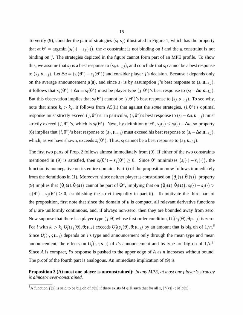
FIGURE 1. Intuition for Prop. 2

Proposition 2 (Monotonicity w.r.t. observable characteristics):† If sss be an MPE, then for allε > 0 and for all i and j such that ki −k j > ε,

i) θ˜

i(sss) ≤ θ˜

j(sss) andθi(sss) ≤ θ j(sss).

ii) si(·) > sj(·) on the interval(θ˜

j(sss), θi(sss)).

Further, there exists N∈ N such thatiii) if n > N and sj is non-degenerate, then si(·) = a.iv) if n > N and si is non-degenerate, then sj(·) = a

¯.

In the discussion of Prop. 2 that follows, we will say that thea (resp.a¯) constraint isbindingon r

at θ if the unconstrained optimal response of playerr of typeθ to sss−r strictly exceeds ¯a (resp. is

strictly less thana¯). Note significantly that by continuity, the ¯a (resp.a

¯) constraint isnot binding

on r at θr(sss) (resp. θ˜

r(sss)). The key to the proof of Prop. 2 is the observation that ifsi andsj

form part of an equilibrium profile, then at any typeθ∗ belonging to the (necessarily nonempty)

setΘ∗ ≡ argmin(si(·)−sj(·)

),

eitherthea constraint is binding oni or thea¯

constraint is binding onj (or both). (9)

-15-

To verify (9), consider the pair of strategies(si,sj) illustrated in Figure 1, which has the property

that atθ∗ = argmin(si(·)− sj(·)

), the a constraint is not binding oni and thea

¯constraint is not

binding on j. The strategies depicted in the figure cannot form part of an MPE profile. To show

this, we assume thatsj is a best response to(si,sss−i, j), and conclude thatsi cannot be a best response

to (sj ,sss−i, j). Let ∆a = (si(θ∗)−sj(θ∗)) and consider playerj ’s decision. Becauset depends only

on the average announcementµ(sss), and sincesj is by assumptionj ’s best response to (si ,sss−i, j),

it follows thatsj(θ∗)+ ∆a = si(θ∗) must be player-type( j,θ∗)’s best response to (si −∆a,sss−i, j).

But this observation implies thatsi(θ∗) cannot be(i,θ∗)’s best response to (sj ,sss−i, j). To see why,

note that sinceki > k j , it follows from A5(ii) that against thesamestrategies,(i,θ∗)’s optimal

response must strictly exceed( j,θ∗)’s: in particular,(i,θ∗)’s best response to (si −∆a,sss−i, j) must

strictly exceed( j,θ∗)’s, which issi(θ∗). Next, by definition ofθ∗, sj(·) ≤ si(·)−∆a, so property

(6) implies that(i,θ∗)’s best response to(sj ,sss−i, j) must exceed his best response to(si −∆a,sss−i, j),

which, as we have shown, exceedssi(θ∗). Thus,si cannot be a best response to(sj ,sss−i, j).

The first two parts of Prop. 2 follows almost immediately from(9). If either of the two constraints

mentioned in (9) is satisfied, thensi(θ∗)− sj(θ∗) ≥ 0. Sinceθ∗ minimizes(si(·)− sj(·)

), the

function is nonnegative on its entire domain. Part i) of the proposition now follows immediately

from the definitions in (1). Moreover, since neither player is constrained on(θ˜

j(sss), θi(sss)), property

(9) implies that(θ˜

j(sss), θi(sss))

cannot be part ofΘ∗, implying that on(θ˜

j(sss), θi(sss)), si(·)−sj(·) >

si(θ∗)− sj(θ∗) ≥ 0, establishing the strict inequality in part ii). To motivate the third part of

the proposition, first note that since the domain ofu is compact, all relevant derivative functions

of u are uniformly continuous, and, if always non-zero, then they are bounded away from zero.

Now suppose that there is a player-type( j,θ) whose first order condition,U ′j(sj(θ),θ;sss− j) is zero.

For i with ki > k j U ′i (sj(θ),θ;sss−i) exceedsU ′

j(sj(θ),θ;sss− j) by an amount that is big oh of 1/n.8

SinceU ′i (·, ·;sss− j) depends oni’s type and announcement only through the mean type and mean

announcement, the effects onU ′i (·, ·;sss−i) of i’s announcement and hs type are big oh of 1/n2.

SinceA is compact,i’s response is pushed to the upper edge ofA asn increases without bound.

The proof of the fourth part is analogous. An immediate implication of (9) is

Proposition 3 (At most one player is unconstrained):In any MPE, at most one player’s strategyis almost-never-constrained.

8A function f (x) is said to be big oh ofg(x) if there existsM ∈ R such that for allx, | f (x)| < M|g(x)|.

-16-

To verify Prop. 3, observe from (9) that ifi is not up-constrained atθ∗ ∈ Θ∗, then j must be down-

constrained. Since by definitionΘ∗ is nonempty, in equilibrium it can never happen that bothsi

andsj are almost-never-constrained. That is, regardless of the width of the announcement spaceA,

an equilibrium cannot exist unless misreporting by all but at most one player increases to the extent

that with positive probability, their announcements are constrained by one of the boundaries. Thus

Prop. 3 highlights the role of the announcement bounds in ensuring the existence of MPE.

The comparative statics results we present in §6 and §7 belowapply only to games with relatively

few players. Props. 2 and 3 suggest why: as the population expands, the tug-of-war between

players with different biases becomes so intense that almost all of them are driven to the boundaries

of the strategy space, resulting in increasingly degenerate outcomes. Prop. 4 below makes this idea

precise. We allown to increase without bound, and demonstrate that in the limit, the outcome of the

game is independent of players’ realized signals. This result contrasts sharply with the recurring

theme in the information aggregation literature, i.e., when the number of participants is very large,

political institutions such as elections can effectively aggregate private information.

Fix a setK ⊂ R from which players’ observable characteristics are drawn and consider a sequence

of finite support measures(φn) on K. For eachn, letkkkn be the support ofφn and let\n be an MPE

of then-player aggregation game with observable characteristic profile kkkn. Let τn : Θ → R be the

induced mapping from mean signals to outcomes, i.e., forθθθ ∈ΘΘΘ, τn(µ(θθθ)) = t(\n(θθθ),kkkn). Prop. 4

establishes that asn→ ∞, the outcome induced by(τn) converges to a constant function.

Proposition 4 (Asymptotic information transmission):† Assume that the measures(φn) con-verge weakly to a nonatomic measureφ on K whose cdf isΦ. Then(τn) converges weakly to theconstant function whose image{k∗} is a convex combination of a

¯anda.

Prop. 4 is a straightforward consequence of parts iii) and iv) of Prop. 2. Asn increases, players

must exaggerate more and more, if they are to exert the same degree of influence over the average

outcome. But there are bounds on how much players can exaggerate, and once these bounds are

attained, the connection between players’ announcements and their signals is broken. It follows

that asn increases, the fraction of players whose strategies conveyany information at all about their

signals shrinks to zero. Because the limit distribution over players is non-atomic, the aggregation

rule assigns vanishingly small weight to the information that these few players provide.

-17-

We conclude this section with a discussion of the class of strategies on which we will focus for the

remainder of the paper. Lettingι(·) denote the identity map onΘ, playerr ’s strategy is said to be

constrained unit affine (CUA)if for someλ ∈ R, sr(·) = min{a,max{a¯, ι(·)+λ}}

unit affineif neither bound on the announcement space is binding, i.e.,if sr(·) = ι(·)+λr

The defining property of a CUA strategy is that the extent ofr ’s mis-representation of his type

is independent of this type, except whenr is constrained by the boundaries ofA. The param-

eter λr indicates the extent of this mis-representation. A CUA strategy is unit affine iff it is

also almost-never-constrained. CUA strategies are a special class of nondegenerate strategies

that play an central role in our analysis. Next, note that theset of degenerate CUA strategies

{sr(·) = min{a,max{a¯, ι(·) + λ}} : λr ≤ a

¯− θ} are all functionally equivalent: in each case,

sr(·) = a¯. Similarly all CUA strategies withλr ≥ a− θ are equivalent. Hence we can impose

without loss of generality (w.l.o.g.) that

sr(·) = min{a,max{a¯, ι(·)+λ}} is anadmissible CUA strategyiff λr ∈ Λ ≡ [a

¯−θ, a−θ]. (10)

Sincea > a¯

andθ > θ, the setΛ is nonempty. Observe from (1a) and (1b) that ifsr is CUA, then

θ˜

r(sr) = min{θ,a¯−λr} < max{θ, a−λr} = θr(sr). (11)

If Θ ⊆ [a¯, a] we say that the announcement space isinclusive. It follows from (11) that

if Θ is inclusive then no CUA strategy is bi-constrained (12)

To see this, note that ifΘ is inclusive andλr ≥ 0 thensr(θ) = θ + λr ≥ a¯+ λr ≥ a

¯; similarly, if

λr ≤ 0 thensr(θ) ≤ a,

4. AGGREGATION GAMES WITH COMMON PREFERENCES

Assumption A1(ii) specifies that all players have distinct observable characteristics. For this sec-

tion only, we reverse this assumption, and consider games inwhich players’ observable character-

istic are identical. We also assume that the announcement space is inclusive, so that truthful type

revelation is feasible. This analysis will serve as a usefulbenchmark when we consider games

-18-

in which players’ observable characteristics are heterogeneous and when the bounds on the an-

nouncement space preclude complete truthful revelation. The analysis highlights the importance

of unit affine strategies: we will show that inn-player games, there are equilibria—including one

characterized by truthful type revelation—in which players’ strategies are unit affine and satisfy a

strong efficiency criterion. Moreover, in two-player games, equilibrium strategies arenecessarily

unit affine, andall equilibria satisfy this criterion.

We now introduce our notion of efficiency. An actionsr(θ) is a best conceivable responsefor

player-type(r,θ) to sss−r if for all sss′−r and alla∈ A, Ur(sr(θ),θ;sss−r)≥Ur(a,θ;sss′−r). When a player-

type’s action is a best conceivable response to other players’ strategies, this player’s expected

payoff could not be higher, even if he had total control over the strategies played by all other

players! An MPE is now defined to beefficientif every player-type’s action is a best conceivable

response to other players strategies. This is clearly an extremely stringent notion of efficiency.

A strategy profile will be calledzero-sum unit affine (ZSUA)if each player’s strategy is unit affine

and if there is truthful revelation in aggregate. Specifically, let ΛΛΛ = {λλλ ∈ Λn : ∑nr=1 λr = 0}. A

strategy profile is ZSUA if for someλλλ ∈ ΛΛΛ, sr = θr +λλλr , for eachr.9 Given a profilesss, µ(sss)

is identically equal toµ(θθθ) iff sss is ZSUA; that is, ZSUA profiles truthfully reveal types in the

aggregate and vice versa. A special case is whenλλλ = 0, i.e., each individual agent reveals his type.

The following proposition highlights the intuitive fact that in an aggregation game, incentives for

strategic behavior arise only when there areex antedifferences between agents’ characteristics,

i.e., theirk’s.

Proposition 5 (ZSUA profiles as equilibrium strategies): Consider an inclusive aggregationgame in which kr = k for all r. A sufficient condition for a strategy profile to be an equilibrium isthat it is ZSUA. Further, a ZSUA equilibrium is efficient.

The proof of Prop. 5 is immediate. Considerλλλ = (λr ,λ−r) ∈ΛΛΛ. Necessarily,λr =−∑i 6=r λr . In the

ZSUA strategy profile corresponding toλλλ, player-type(r,θ) reportssr(θ) = θ+λr . Consequently

Ur(sssr(θ),θ;sss−r) =

∫

ΘΘΘ

u(t(sss(ϑϑϑ),kkk),ϑϑϑ, k)η(ϑϑϑ)dϑϑϑ =

∫

ΘΘΘ

u(t(ϑϑϑ,kkk),ϑϑϑ, k)η(ϑϑϑ)dϑϑϑ

9Clearly, for any vectorλλλ with λr < (a¯− θ) (or λr > a− θ), sr = θr +λλλr would not be admissible for types in some

neighborhood ofθ (or θ).

-19-

Since players’ observable characteristics are all identical, the social welfare function (defined in

(2)) coincides with each player’s utility function:w(t,θθθ,kkk) = u(t,θθθ, k). Since the outcome function

is assumed to be CISE, we havet = argmaxu(·,θθθ, k) for everyθθθ ∈ ΘΘΘ, Thus, the ZSUA profile

maximizes the expected utility of every player and constitutes an MPE. Further, since each player

obtains the highest possible utility, the equilibrium is also efficient.

When there are only two players with identical observable characteristics, we can go much further.

In this case, the preceding and following propositions establish that a profile is an equilibrium if

and only if it is ZSUA, i.e.,all equilibria are efficient!10

Proposition 6 (MPE are ZSUA):† Consider a two player inclusive aggregation game with ki = k j .A necessary condition for a strategy profile to be an MPE is that it is ZSUA.

θ θ

si(·) si(·)si(·)

sj(·) sj(·)si(θ∗i )

sj(θ∗j ) sj(θ∗j )

λ

λ λ

45deg 45deg

θ∗i θ∗j

sj(θ∗j ) = θ∗j −λ

si(θ∗i ) = θ∗i +λ

stra

teg

ies

stra

teg

ies

θ∗i + ι(·)θ∗j + ι(·)

ι(·)ι(·)

θ θ

si(θ∗i )+sj(·)

sj(θ∗j )+si(·)

FIGURE 2. Intuition for Prop. 6

Figure 2 provides some intuition. Consider a strategy that is not unit affine, such assj in the left

panel of the figure. Lettingι(·) denote the identity map, the maximum value of(ι(·)−sj(·)) is λ,

which is achieved uniquely atθ∗j .11 We first establish that a necessary condition forsi to be a best

response tosj is that(si(·)− ι(·)) is everywhere strictly less thanλ. To see this, consider a strategy

such as ˆsi satisfying, for someθ∗i , (si(θ∗i )−θ∗i ) ≥ λ. Given any such strategy fori, the aggregate

strategy ˆsi(θ∗i )+ sj(·)—i.e., the highest curve in the left panel—must lie above theline θ∗i + ι(·)

10An immediate implication of the argument below is that when players’ observable characteristics are identical andthe announcement space coincides withΘ, then theuniqueequilibrium for a two-player aggregation game is thatplayers truthfully reveal their private information with probability one.11Uniqueness is not required, but it simplifies the intuitive exposition.

-20-

with probability one. That is, for player-type(i,θ∗i ), the average of players’ announced types

exceeds the average of their actual types with probability one. Sincet(·) is CISE and the social

welfare functionw(·) coincides withi’s and j ’s common utility function, the outcome generated

by (sj , si) must be super-optimal for(i,θ∗i ) with probability one. Conclude thatθ∗i +λ is not a best

response for(i,θ∗i ) againstsj(·); more generally, forsi to be optimal against any not unit affine

sj , it is necessary that(si(·)− ι(·)) < max(ι(·)−sj(·)). Now consider any strategy satisfying this

necessary condition—e.g., the dashed curvesi(·) in the right panel—and observe that the aggregate

strategysj(θ∗j )+si(·) is everywherebelowthe lineθ∗j + ι(·), and hence sub-optimal for( j,θ∗j ). We

have shown, then, that the actionsj(θ∗j ) cannot be a best response for( j,θ∗j ), againstanystrategy

that could possibly be a best response against the arbitrarily chosen, not unit affinesj(·).

5. GAMES WITH QUADRATIC PAYOFF FUNCTIONS

In our introductory discussion in §1, our players reported to the center, who took an action,τ, that

affected all of them. For the remainder of the paper, we abstract from the issue of how the center

uses the information that players provide and assume, simply, that each player incurs a loss that

is quadratic in the difference between that player’s observable characteristic and the gap between

the means of actual and reported information. Formally, we define the utility function for a player

with observable characteristick as the biased quadratic loss function:12

u(τ,µ(θθθ) ,k) = −(k+µ(θθθ)− τ)2 . (13)

With this specification, the CISE property requires the center to average the types that players an-

nounce:τ = t(sss,kkk) = µ(sss). A game with utilities given by (13) will be called aquadratic aggrega-

tion game. It is straightforward to verify that givent, (13) satisfies Assumptions A4-A6. The goal

of a player with observable characteristick > 0 is to induce the center to overestimate the value of

µ(θθθ) by an amount that is as close as possible tok. Specifically, the optimal expected outcome for

a player with observable characteristickr and type parameterθr is Eϑϑϑ−r t = kr +Eϑϑϑ−r µ(〈θr ,ϑϑϑ−r〉).

This quadratic specification is consistent with either of the two interpretations of our model pro-

posed in §1. For the non-statistical interpretation, the relationship is self-evident: players lose util-

ity with the square of the difference between the composite score implied by players’ actual types,

adjusted by the player’s personal bias, and the score that the center would compute by aggregat-

ing players’ announcements. Under the Bayesian interpretation, each player loses utility with the

12As noted in fn. 1, this specification is very widely used.

-21-

square of the difference between the posterior mean computed by the center from announcements

and the one implied by actual types, again after adjusting for the player’s bias. Under very general

conditions, the posterior mean is an affine function of the sample mean.13 If the posterior mean is

defined asb0+b1µ(θθθ), the loss function implied by our Bayesian interpretation is

−(k+(b0+b1µ(θθθ))− (b0+b1µ(sss))

)2= −

(k+b1(µ(θθθ)−µ(sss))

)2= −

(k+b1(µ(θθθ)− τ)

)2.

By choosing appropriately the units of the vectorkkk, we can setb1 = 1 and recover (13).

While this Bayesian interpretation is suggestive, there isa notable distinction between our qua-

dratic loss function and the canonical Bayesian loss function. To best appreciate the difference,

consider (13) for an unbiased player, i.e., setk = 0. Then the only source of loss is that players

mis-report the signals they receive; our players are modeled as uninterested in the difference be-

tween the mean of their signals and thetruemean of the distribution from which their signals were

drawn. In the classical Bayesian problem, on the other hand,the latter difference is all that matters;

the possibility of mis-reporting does not arise.

In most respects, this distinction is unimportant and our specification captures exactly what we are

interested in, i.e., the information losses that arise because players are strategic and are constrained

by the boundaries.14 In one respect, however, the omitted difference is significant: in a game

small enough to admit non-degenerate strategies, it does not capture the full welfare impact in a

Bayesian setting of increasingn, since it ignores the welfare benefit of increasing the precision

with which the aggregate signal estimates the true mean (i.e., reducing the second term in (14)).

As an extreme example, when all players have the same observable characteristic as in §4, our

players attain Nirvana in every game, regardless ofn; had we defined players’ utility as a standard

Bayesian loss function, Nirvana would be approached only asymptotically.

13Bernardo and Smith (2000, Proposition 5.7 (pp. 275-276)) establishes this for exponential families of distributions.14 For instance, if theθi ’s were independently drawn from a distribution withE(θi) = θt and players’ utility dependedon the true meanθt rather than the average realized signalµ(θθθ), the expected quadratic loss would be

−E(k+ θt − τ)2 ≡ −Eϑϑϑ(k+µ(ϑϑϑ)− τ+ θt −µ(ϑϑϑ))2 = −Eϑϑϑ(k+µ(ϑϑϑ)− τ)2−Eϑϑϑ(θt −µ(ϑϑϑ))2. (14)

The first part of the loss arises entirely due to misreportingand coincides withu(·) in (13); the second part, which isprecisely the canonical Bayesian loss function, is omittedfrom our model.

-22-

5.1. CUA strategies. The quadratic specification ensures that equilibrium strategies will be CUA

(see p 17). Given the utility (13) and outcome functiont(sss,kkk) = µ(sss), if r were not required to

respect the admissibility bounds (10) onλr , his optimal response tosss−r would be the UA strategy

θr +λr , where

λr = nkr +∑i 6=r

Eϑi (ϑi −si(ϑi)) . (15)

In general, the UA responseθr +λr will not belong toA for all values ofθr , particularly if |kr | is

large. Accordingly,r ’s constrainedoptimal response will be

sr(θr) = min{a,max{θr +λr ,a}}. (16)

To identify an NMPE, we need to compute theλλλ vector which solves the set ofn equations in (15)

subject to the constraint (16). As a first step, we letξr(·) denote playerr ’s deviation from affine,

defined as the difference between the CUA strategysr(·) and the UA strategyι(·)+λr. Givenλr ,

let Eξr denoter ’s expected deviation from affine:

Eξr ≡ Eϑr (sr(ϑr)− (ϑr +λr)) = Eϑr

(min{a,max{a

¯,ϑr +λr}}−ϑr

)− λr (17)

=∫ θ

˜r

θ(θ˜

r −ϑr)dH(ϑr) +∫ θ

θr

(θr −ϑr)dH(ϑr), (18)

where, from (1a) and (1b),θ˜

r(λr) = a¯− λr and θr(λr) = a− λr . ThusEξr is a measure of the

impact of the bounds ¯a anda¯

on r ’s expected announcement. Clearly,

if r is single-constrained andEξr 6= 0, λrEξr < 0. (19)

Since we focus exclusively on CUA strategies in the remainder of the paper, we will sometimes

use the symbolλr as a shorthand for the uniquely defined CUA strategy with parameterλr .

We note in passing two implications of (17) and (18) that we will use later. First, aggregating the

identity in (17) across players and rearranging, we obtain

Eϑϑϑ(µ(sss∗(ϑϑϑ)) − µ(ϑϑϑ)

)= µ(λλλ∗) + µ(Eξξξ) . (20)

Second, differentiating (18) w.r.t.λr and inferring from (11) thatH(θ˜

r) < H(θr):

-23-

dEξr

dλr= −

(H(θ

˜r) + 1 − H(θr)

)⊂ (−1,0] (21)

anddEξr

dλr= 0 iff r is almost never constrained

Substitutingθi −si(θi) = −(λi +ξi) into (15) and rearranging, it follows that ifλλλ∗ is an MPE,

nkr = ∑i

λ∗i + ∑

i 6=r

Eξi(λ∗i ), for all r with λ∗

r ∈ int(Λ). (15′)

Figure 3 provides some intuition for (15′), for the simple game with two playersi and j and

0 < ki = −k j . The figure is a diagonal cross-section of the three-dimensional graph fromΘ×Θ

to outcomes, that is, the graph depicts the event thati and j observe the same private signals.

Playeri is up-constrained while playerj is down-constrained. The thick kinked line represents

������������������������������������������������������������������

������������������������������������������������������������������

������������������������������������������������������������

������������������������������������������������������������

signal

outcome

player types

i’s strategy

j ’s strategy

i’s ideal outcome

Area=|Eξ j(λ j)| = 2ki

θ θ

a

a¯

θi

θ˜

j

FIGURE 3. Intuition for display (15′)

the outcome as a function of type realizations, given the twoplayers’ strategies. The important

property highlighted by the kinked line is that whenθi > θi (andθ j ∈ [θ˜

j , θ j ]), the realized outcome

is an under-estimate of the realized type, while whenθ j < θ˜

j (and θi ∈ [θ˜

i , θi]), it is an over-

estimate; whenθr ∈ [θ˜

r , θr ], for r = i, j, the outcome accurately reflects the aggregate signal. Now

consider the outcome from playeri’s perspective and for concreteness, supposeθi = 0 and the

horizontal axis representsj ’s type. Playeri’s ex posteideal outcome, as a function ofj ’s type,

is represented by the dashed line above the diagonal: for every value of j ’s type, i’s ex poste

-24-

ideal outcome exceeds it byki . When j is unconstrained, his under-report exactly counteracts

i’s over-report, resulting in an outcome that is suboptimal from i’s perspective; however, at low

values ofθ j , the constrainta¯

binds j ’s under-reporting, resulting in an outcome exceedingi’s ideal

outcome. Equation (15′) describes how the over- and under-estimates are balanced in equilibrium:

the expected over-estimate of the true average equals twicethe expected under-estimate.

The following, immediate implication of (15′) will prove very useful in what follows. Ifλλλ∗ is an

MPE, then for alli, j with λ∗i ,λ∗

j ∈ int(Λ),

n(ki −k j) = Eξ j(λ∗j ) − Eξi(λ∗

i ). (22)

To motivate (22), supposeki > k j and bothi and j are up-constrained. From part ii) of Prop. 2,

ki > k j impliesλi > λ j , so the constraint ¯a binds more tightly oni than onj, i.e.,Eξi < Eξ j .

Proposition 7 (Uniqueness of MPE):† Every quadratic aggregation game has a unique MPE.

5.2. MPE outcomes and payoffs.The quadratic setup allows us to analyze each player’s equi-

librium performance: to what degree the outcome of the game matches his ideal outcome, and

how his payoff depends on player characteristics. We begin by introducing a notion describing

the degree to which each player “gets what he wants” in equilibrium. We define as a benchmark

the complete information personally optimal (CIPO) outcomefor player r: this outcome would

maximizer ’s payoff if he had complete information about the average type. We denote this “ideal”

outcome fromr ’s perspective byt(θθθ,kr). From (13),r ’s CIPO outcome is

t(θθθ,kr) = µ(θθθ)+kr . (23)

If µ(sss∗) is the equilibrium outcome of the game. then the differenceEϑϑϑ(µ(sss∗(ϑϑϑ))

)− t(ϑϑϑ,kr)

),

which we label asr ’s expected CIPO deviation, is a measure of the degree to which the equilibrium

outcome differs in expectation from playerr ’s CIPO outcome. Prop. 8 below establishes that in

an NMPE, the expected CIPO deviation is 1/n times the size of the player’s expected deviation

from affine. This result is striking because the latter depends only onr ’s strategic choice, while the

former depends onall players’ choices. Note also from (19) that a single-constrained player who

over- (under-) reports his type can expect a sub- (super-) optimal outcome.

Proposition 8 (The expected CIPO deviation):† If sss∗ = θθθ+λλλ∗ is an MPE profile of a quadraticaggregation game, andλ∗

r ∈ int(Λ), then r’s expected CIPO deviation is Eξr(λ∗r )/n.

-25-

Since the expected deviation from affine measures how tightly the announcement bounds restrict

r ’s action in equilibrium, Prop. 8 indicates that a player whose action is more restricted is less

likely to obtain his CIPO outcome in expectation.

After r learns his typeθr , a parallel measure of deviation from his ideal outcome is the interim

expected CIPO deviation, defined as the differenceEϑϑϑ−r

(µ(〈s∗r (θr),sss

∗−r(ϑϑϑ−r)〉)− t(〈θr ,ϑϑϑ−r〉,kr)

),

whereEϑϑϑ−r t(〈θr ,ϑϑϑ−r〉,kr) = Eϑϑϑ−r µ(〈θr ,ϑϑϑ−r〉)+kr is r ’s interim expected CIPO outcome. Similar

to Prop. 8, Prop. 9 establishes thatr ’s interim expected CIPO outcome is implemented in equilib-

rium if and only if his strategy is unconstrained atθr :

Proposition 9 (Interim Implementation): † For a player r of typeθr , his interim expected CIPOdeviation equals zero, or his interim expected CIPO outcomeis implemented in equilibrium, if andonly if his strategy s∗r is unconstrained atθr .

The previous discussion indicates that playerr ’s expected deviation from affine i.e., the expected

degree to whichr ’s strategies are restricted by the announcement bounds, isinstrumental in deter-

mining whetherr gets “what he wants.” We next illustrate how the deviation from affine affects

a player’s expected equilibrium payoff. From (13),r ’s expected payoff from a strategy profileλλλ

is −Eϑϑϑ (µ(ϑϑϑ)+kr −µ(sss)))2, i.e., the expectation of the squared difference betweenr ’s CIPO out-

come and the realized outcome. For an arbitrary profileλλλ, the expression for this expectation is

exceedingly messy, reflecting the complexity of the interactions between multiple players’ devia-

tions from affine: in some regions ofΘΘΘ, the distortion resulting from different players’ constraints

offset each other; in others they are mutually reinforcing.In equilibrium, however,all of these

interaction terms disappear, leaving only the first and second moments of players’ deviations from

affine. Specifically, letVξr(λr) denote the (ex ante) variance ofr ’s deviation from affine, i.e.,

Vξr(λr) = Varϑ(sr(ϑr)− (ϑr +λr)

)(24)

Note thatVξr(λr) depends only onr ’s own type realization. We now have:

Proposition 10 (Equilibrium Payoffs):† Letsss∗ = θθθ+λλλ∗ be an MPE profile of a quadratic aggre-gation game. For each player r withλ∗

r ∈ int(Λ), r’s expected equilibrium payoff is

Eϑϑϑu(µ(sss∗),µ(ϑϑϑ) ,kr) = −Eϑϑϑ(µ(ϑϑϑ)+kr −µ(sss∗)

)2= −

(µ(VξVξVξ(λλλ∗))/n + (Eξr(λ∗

r )/n)2) . (25)

Prop. 8 and Prop. 10 are complementary. Prop. 8 established that playerr ’s expected CIPO devi-

ation coincides with his expected deviation from affine, deflated byn. But equilibrium expected

payoffs depend onsquareddeviations from affine. Prop. 10 shows that players’ expected payoffs

-26-

are equally negatively impacted by the variances of each others’ deviation from affine; the sole fac-

tor distinguishing two players’ expected payoffs is the difference between their squared expected

CIPO deviations.

We next study the aggregate equilibrium payoff of the players. From a normative perspective, there

are two benchmark measures of welfare that we might consider. The more obvious is the average

of players’ equilibrium expected payoffs. We refer to this asaverage private welfare, defined as

APW =1n

Eϑϑϑ

(n

∑i=1

u(µ(sss),µ(ϑϑϑ) ,ki)

). (26)

Alternatively, one could take the view thatsocial welfare should be evaluated from anunbiased

perspective, i.e., from the perspective of a player whose observable characteristic is zero, reflecting

a preference for truthful revelation. Accordingly we defineunbiased social welfareas

USW = Eϑϑϑu(µ(sss),µ(ϑϑϑ),0) = Eϑϑϑ (µ(ϑϑϑ)−µ(sss))2 . (27)

Our assumption that∑i ki = 0 implies that APW and USW differ only by a constant. Specifically:

APW = − 1n

Eϑϑϑ ∑i∈I

(µ(ϑϑϑ)+ki −µ(sss))2

= − 1n

{

∑i

k2i + 2∑

ikiEϑϑϑ (µ(ϑϑϑ)−µ(sss)) + nEϑϑϑ (µ(ϑϑϑ)−µ(sss))2

}

= USW + ∑i

k2i /n

From (47) the following result is immediate.

Proposition 11 (Unbiased Social Welfare): If λλλ∗ is an MPE profile of a quadratic aggregationgame, then unbiased social welfare is given by

USW = −{

µ(Vξξξ(λλλ∗))/n +(µ(Eξξξ(λλλ∗))+µ(λλλ∗)

)2}(28)

5.3. Anchored Games.The discussion so far illustrates the central role the expected deviation

from affine plays in affecting equilibrium payoffs. There isa class of games in which some player

j ’s expected deviation from affine is zero. This property holds if either j ’s strategy is never con-

strained or if the constraints onj associated with the two announcement bounds cancel each other

-27-

out in expectation. We later study games in which such aj always exists: in §6,j is the “middle”

player in a symmetric game; in §7, the “largest” player in a game in whicha never binds. We

refer to such a game as ananchored gameand to playerj as the anchor. Anchored games are

particularly easy to solve and exhibit strong properties.

Proposition 12 (Properties of anchored games): Let λλλ∗ be an MPE profile of an anchoredquadratic aggregation game and let j be the anchor. For each player r withλ∗

r ∈ int(Λ),i) r’s expected deviation from affine is n(k j −kr),

ii) r’s expected CIPO deviation is(k j −kr),

Part i) is obtained by combining (22) with the defining property of an anchored game, i.e.,Eξ j(λ∗j ) =

0. Part ii) then follows from Prop. 8. Strikingly,r ’s expected CIPO deviation depends exclusively

on the gap betweenj ’s observable characteristic andr ’s, while r ’s expected deviation from affine

depends both on this gap andn. To see why the latter is proportional ton, recall thatr ’s objective

is to shift the mean announcement by a magnitudekr that is independent ofn; the greater isn, the

smaller isr ’s contribution to the mean, and hence the more mustr mis-report. Note that the more

r mis-reports, the more likely it is that he will be constrained by the announcement bounds. To

study anchored games, we add assumption A7 to A1-A6. Parts (i) and (ii) simplify our anlysis.

Part (iii) ensures that every anchored game has an NMPE.

Assumption A7: (i) The announcement space is inclusive (cf. p. 17); (ii) thetype distribution isuniform with density parameterη = 1/(θ−θ); (iii) ||kkk||∞ < (θ−θ)/4n.

A7(ii), combined with (13), yields the widely used “uniformquadratic” specification.15 The benefit

of the uniformity assumption is its tractability; the cost is that it is inconsistent with the Bayesian

interpretation of our model16. Our alternative, non-statistical interpretation does, however, remain

valid. A7(iii) guarantees that our MPE is non-degenerate: if there are a large number of players

and thek’s are far apart, extreme players, in trying to steer the average announcement in his favor,

might choose such extreme strategies that are always constrained by one of the announcement

bounds, i.e., strategies that are degenerate. To verify non-degeneracy, it suffices to check that

Eξr(λ∗r ) = n(k j −kr) is consistent withλ∗

r ∈ int(Λ). Assuming w.l.o.g. thatλ∗r > 0, (18) implies:

Eξr(λ∗r ) =

∫ θ

a−λ∗r

(ϑr +λ∗r − a)dη(ϑr) = 0.5η

(λ∗

r +θ− a)2

so that λ∗r +θ− a =

√2η

Eξr =

√2η

n(k j −kr) if λ∗r ∈ int(Λ). (29)

15See Gilligan and Krehbiel (1989), Krishna and Morgan (2001), Morgan and Stocken (2008), and many others.16See the discussions on pp. 2-3 and p. 21

-28-

The last equality follows from Prop. 12. Also, from A7(iii),

2n(k j −kr)/η ≤ 4nη||kkk||∞ <

4nη

(θ−θ)/4n = (θ−θ)2

so thatλr =√

2ηn(k j −kr)− (θ− a) <

((θ−θ)− (θ− a)

)= a−θ, verifying thatλ ∈ int(Λ).

For anchored games satisfying A7, we obtain a closed-form expression for equilibrium payoffs.

Proposition 13 (Equilibrium Payoffs in Anchored Games):† Let j be the anchor in an anchoredquadratic game satisfying A7. Then player r’s equilibrium expected payoff is

Eϑϑϑu(µ(sss∗),µ(ϑϑϑ) ,kr) = −{

n

∑i=1

(k j −ki)2

(√8

9nη|k j −ki |− 1

)+(kr −k j)

2

}(30)

≤ −{

n

∑i=1

(k j −ki)2/3+(kr −k j)

2

}.

Expr. (30) thus establishes an upper bound on expected payoffs that declines withn. As shall see

below, however, this doesnot imply that expected payoffs themselves decline monotonically. In

the following sections, we study how the equilibrium outcome and aggregate welfare are related

to primitives of the game such as the vectorkkk and the bounds ¯a anda¯. For an arbitrary quadratic

game, it is impossible to obtain closed-form expressions for these effects. Accordingly, we will

focus on two special classes of anchored games for which closed-form results can be obtained.

6. SYMMETRIC GAMES

In this section we study games which are symmetric in a strongsense. We say that the observable

characteristic vector is symmetric if for every player ¯r with kr > 0, there exists amatched player r

with kr =−kr . There may in addition be one more,middleplayermwith km = 0. In §6.4 below, we

will refer to players whose observable characteristics arepositive (resp. negative) as theright-wing

(resp. left-wing) faction. We say that the announcement space is symmetric if the announcement

boundsa¯

anda are symmetric about zero, i.e., ifa¯= −a; finally, we say that the type distribution

is symmetric ifθ = −θ and if θ is symmetrically distributed around its mean zero. We now say

that a game issymmetricif all these conditions are satisfied. A1-A7 are satisfied throughout the

section, unless an exception is explicitly indicated.

Proposition 14 (MPE of Symmetric Games):† Every symmetric quadratic aggregation game hasa unique MPE satisfying: Eξr(λ∗

r ) = −nkr , for all r with λr ∈ int(Λ). Moreover,i) for each playerr and matched player r, λ∗

r = −λ∗r ;

-29-

ii) if there is a middle player m, thenλ∗m = 0.

The middle player, if there is one, is the only player who announces truthfully in equilibrium. Any

other player always mis-announces and his expected deviation from affine is determined entirely

by his observable characteristic andn. Symmetric games with a middle player are also anchored

games (see §5.3). It is clear from Props. 14 and 8, however, that symmetric games without a middle

player exhibit the same properties as those that have one. Tostreamline the exposition, we shall in

the remainder of the section treatall symmetric games as if they were anchored.

It is immediate from Props. 10 and 14 thatr ’s equilibrium expected payoff is entirely determined

by kr and the average of the second moments of all players’ deviations from affine.

Eϑϑϑu(µ(sss∗),µ(ϑϑϑ) ,kr) = −(µ(Vξξξ)/n + k2

r

)= −

{

∑i

k2i

(√8

9nη|ki |− 1

)+k2

r

}. (25′)

The second equality is obtained by substituting zero fork j in (30). (27) and (25′) now yield an

expression for unbiased social welfare:

USW = −∑i

k2i

(√8

9nη|ki|− 1

)(31)

Prop. 14 provides us with a powerful tool for analyzing and comparing the welfare properties of

aggregation games with different parameters. The three parameters we study in the remainder of

this section are: the number of players (§6.1); the magnitude of the bound on the announcement

space (§6.2); and the heterogeneity of players’ observablecharacteristics (§6.3). Throughout this

section, whenever we make a statement relating to eitherθ, a, orkr , we will be implicitly making as

well the matching statement aboutθ, a¯, or kr . In particular, when we study the effect of increasing

a, we will be simultaneously, but implicitly, reducinga¯

to preserve symmetry.

6.1. Effects of changing the number of players.Since symmetric games are anchored, at least

some of the impacts of changingn are straightforward: a player’s strategy (although not hispayoff)

depends only onn and his own observable characteristic. From Prop. 12, a player’s expected

deviation from affine is proportional ton, while his expected CIPO deviation is independent of

n: asn increases, each player except the middle one mis-reports toan increasing extent, while in

equilibrium the net expected effect of players’ distortions on the center’s decision is unchanged.

-30-

The effects ofn on expected payoffs and welfare are more complex. While in general there is

no closed-form expression forVξr , A7 allows us to obtain determinate results. We will compare

expected payoffs and welfare for a finite sequence of “comparable” games with more and more

players. To make the games comparable, we relax assumption A1(ii) for the remainder of §6.1 and

construct our sequence by cloningm times a base game withqplayers and observable characteristic

vectorκκκ.17 To ensure that A7(iii) is satisfied, we require thatm≤ M = b1/(4qη||κκκ||∞)c.18 Now

consider the aggregate welfare USW(m) in them’th game. Since from (31) and (25′), the difference

between USW(m) and playerr ’s expected payoff is independent ofm, the comparative statics

results we obtain for welfare apply also to payoffs. Rewriting (31):

USW(m) = −mq

∑i=1

κ2i

(√8

9mqη|κi|− 1

)=

q

∑i=1

mκ2i −

√8m|κi|3

9qη

(31′)

If m were a real number rather than an integer, USW would be convexin m, with

dUSWdm

=q

∑i=1

(κ2

i −√

2|κi|3/

(9mqη)

)(32)

The i’th element of the summation isR 0 as|κi| R 2/(9mqη). Let M′ = max{m≤ M : ||κκκ||∞ <

2/(9mqη)} andM′′ = max{m∈ N : |κi| < 2/(9mqη),∀i}; If ηM is sufficiently small,M′ < M

(since 2/9 < 1/4) while if, in addition, maxi |κi| −mini |κi| is sufficiently small,(M′′,M] will be

non-empty. Clearly, USW(·) is strictly decreasing on[1,M′) and strictly increasing on(M′′,M].

These results reflect the tension between two effects asm increases. The first is that players need

to mis-report more to accomplish the same expected CIPO deviation; this lowers welfare. The

second effect reflects the law of large numbers: asm increases, it becomes increasingly likely that

players’ deviations from the mean of the type distribution will offset each other, and hence their

individual deviations from affine will be mutually offsetting also. Prop. 15 summarizes:

Proposition 15 (Comparative statics w.r.t.n): In a symmetric quadratic aggregation game.

i) each original player’s expected deviation from affine is proportional to n.ii) each original player’s expected CIPO deviation is independent of n

17The argument below could be made rigorous without violatingassumption A1(ii): simply clone as we propose, andthen perturb the cloned vector slightly to ensure uniqueness while preserving symmetry. In our view, the loss of rigorinvolved in our approach is justified by the gain in parsimony.18For x∈ R, bxc denotes the greatest integer not exceedingx. For m≤ M, the game withm clones ofκκκ hasn = mqplayers. so that||κκκ||∞ ≤ 1/(4mqη) = (θ−θ)/4n, verifying that A7(iii) is satisfied.

-31-

For a finite sequence of games obtained by cloning m times a vector κκκ ∈ Kq;i) USW and expected payoffs are convex with respect to the number of clones

ii) Suppose||κκκ||∞ < (θ− θ)/4n, i.e., the players are relatively homogenous intheir observable characteristics. Then USW and player expected payoffs ini-tially decrease, and then may increase, with the number of clones.

To reiterate, these results should be evaluated in the context of the non-statistical interpretation of

our model, rather than the Bayesian one (see pp. 2-3 and p. 21).

6.2. Effects of changing the announcement bounds.From Prop. 14, playerr ’s expected devia-

tion from affine,Eξr(·), is independent of the announcement bound ¯a. If kr 6= 0, expression (18)

then implies that as ¯a changes,λr must adjust so thatEξr(·) remains equal tonkr . Specifically:

Proposition 16 (Effects of changinga):† In a symmetric quadratic aggregation game,

dλr

da=

0 if r is the middle player

1 if r is up-constrained

−1 if r is down-constrained(1−H(θr ))−H(θ

˜r)

H(θ˜

r)+(1−H(θr))if r is bi-constrained

(33)

Whenr is bi-constrained, the denominator ofdλrda is the probability thatr is constrained by at least

one of the announcement bounds. The numerator is the difference between the probabilities thatr

is up- and down-constrained. Ifr is single-constrained, he increases the degree of his misreporting

at exactly the rate that the bounds are relaxed; he responds more slowly if he is bi-constrained.

We now consider the welfare effect of a marginal change in theannouncement bound. First note

that if the announcement space is inclusive, no player will be bi-constrained in equilibrium. Then

players withk 6= 0 will adjust their announcements to fully compensate for any change in the

announcement bounds. Hence, players’ utilities, as well asaggregate welfare, will be unaffected

by any change in the bounds. Specifically, recall from Prop. 10 thatr ’s expected payoff depends

on the first moment ofr ’s own deviation from affine, as well as the second moments of all players’

deviations. If there is a middle playerj, ξ j = 0 always and thusEξ j andVξ j are unaffected by

changes in ¯a. For any other playerr, since the change inλr fully compensates the change in ¯a, the

deviation from affineξi (or its distribution) remains unchanged, so do its first and second moments.

-32-

This independence property no longer holds when at least oneplayer’s equilibrium strategy is bi-

constrained. For some intuition for this difference, Figure 4 considers the impact of relaxing the

announcement bounds, when the only bi-constrained player is the middle player,m. Wheneverm’s

type lies outside the interval[a¯, a], obliging him to mis-report his type, all players are negatively

impacted. The areas of the large triangles at either end of the type spectrum indicate the magni-

tude of the distortion. When the bounds are relaxed to[a¯′, a′], the sizes of these triangles shrink,

reflecting a decline in the variance ofm’s deviation from affine. Ex ante, this change benefits all

players equally, since, from Prop. 10, each player’s payoffis decreasing in thetotal variances of

all players. Prop. 17 provides an expression for the rate at which a bi-constrained player’s variance

declines with a relaxation of the bounds. The more players are initially bi-constrained, the greater

is the collective benefit of a relaxation.

Proposition 17 (Effects of increasing the announcement bound a):† In a symmetric quadraticaggregation game, as the announcement space expands:

i) if initially the announcement space is inclusive, the equilibrium expected pay-off of every player remains constant;

ii) if initially some player is bi-constrained, then each player’s equilibrium ex-pected payoff is equally positively affected, as is unbiased social welfare.Specifically, letting I∗ denote the set of players who are bi-constrained inequilibrium, player r’s expected payoff increases by− 1

n2 ∑i∈I∗dVξida , where

dVξi

da=

4

H(θ˜

i)+(1−H(θi))×

{(1−H(θi))

∫ θ˜

i

θ(ϑi −θ

˜i)dH(ϑi) − H(θ

˜i)

∫ θ

θi

(ϑi − θi)dH(ϑi)

}< 0 (34)

Prop. 17 delivers a clear policy message, at least in the context of symmetric games. Recall from

(12) that a necessary condition for a player to be bi-constrained is that the type space is not a

subset of the announcement space. When, as in the present paper, the type space is known by the

policy-maker who sets the announcement bounds, it is Paretooptimal to select an announcement

space large enough to contain the type space. More generally, of course, the bounds on the type

space will not be known with certainty. In this case, since itis costless to expand the announcement

space, and possibly costly to contract it, the announcementspace should be as large as possible.

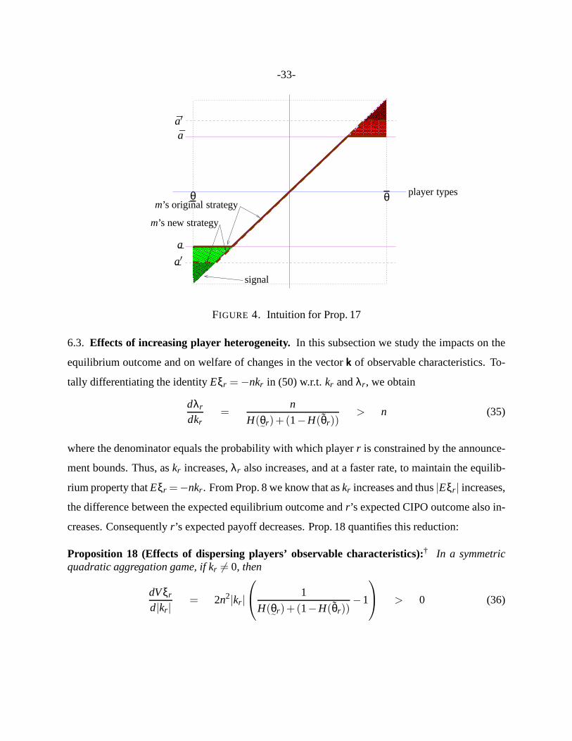
-33-

������������������������������������������������������������������������

������������������������������������������������������������������������

�����������������������������������������������������������������������������

�����������������������������������������������������������������������������

����������������������������

����������������������������

���������������������

���������������������

signal

player typesm’s original strategy

m’s new strategy

θ θ

a′

a¯′

a

a¯

FIGURE 4. Intuition for Prop. 17

6.3. Effects of increasing player heterogeneity.In this subsection we study the impacts on the

equilibrium outcome and on welfare of changes in the vectorkkk of observable characteristics. To-

tally differentiating the identityEξr = −nkr in (50) w.r.t.kr andλr , we obtain

dλr

dkr=

n

H(θ˜

r)+(1−H(θr))> n (35)

where the denominator equals the probability with which player r is constrained by the announce-

ment bounds. Thus, askr increases,λr also increases, and at a faster rate, to maintain the equilib-

rium property thatEξr =−nkr . From Prop. 8 we know that askr increases and thus|Eξr | increases,

the difference between the expected equilibrium outcome and r ’s expected CIPO outcome also in-

creases. Consequentlyr ’s expected payoff decreases. Prop. 18 quantifies this reduction:

Proposition 18 (Effects of dispersing players’ observablecharacteristics):† In a symmetricquadratic aggregation game, if kr 6= 0, then

dVξr

d|kr |= 2n2|kr |

1

H(θ˜

r)+(1−H(θr))−1

> 0 (36)

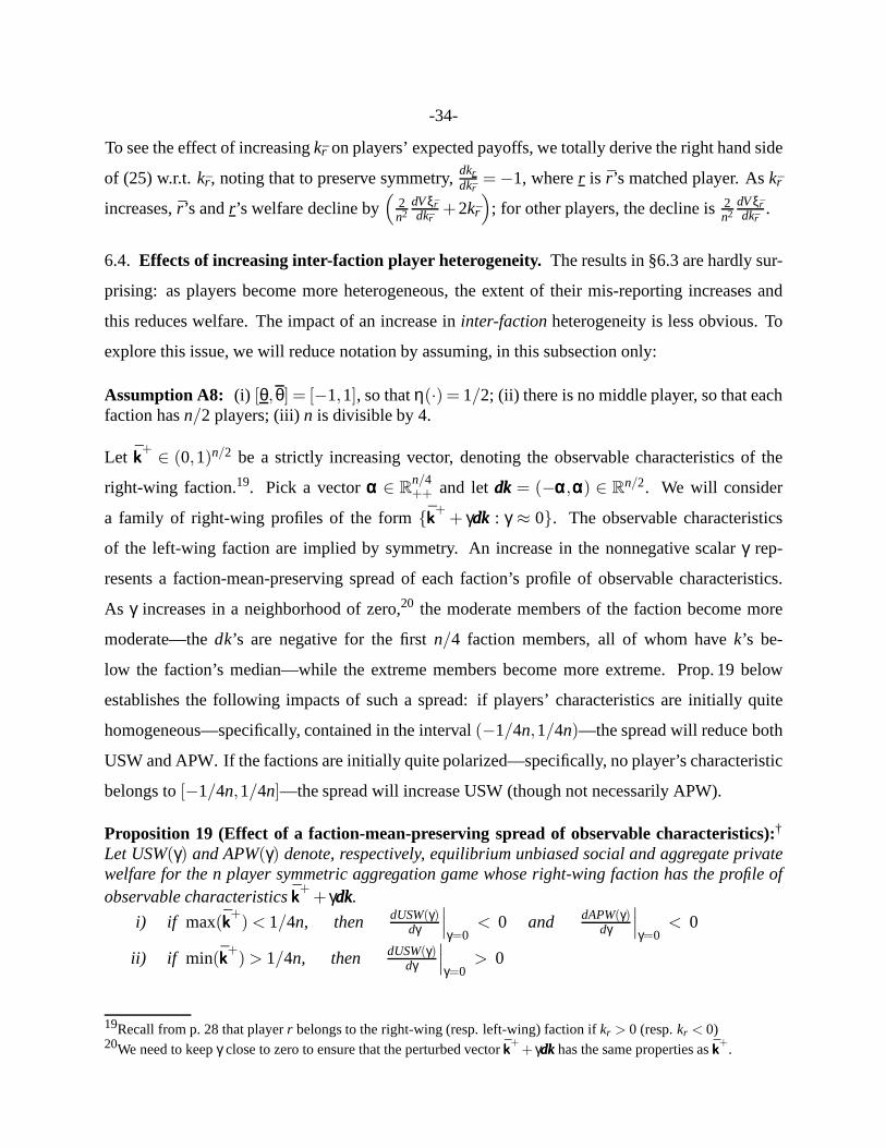
-34-

To see the effect of increasingkr on players’ expected payoffs, we totally derive the right hand side

of (25) w.r.t. kr , noting that to preserve symmetry,dkrdkr

= −1, wherer is r ’s matched player. Askr

increases, ¯r ’s andr’s welfare decline by(

2n2

dVξrdkr

+2kr

); for other players, the decline is2

n2dVξrdkr

.

6.4. Effects of increasing inter-faction player heterogeneity. The results in §6.3 are hardly sur-

prising: as players become more heterogeneous, the extent of their mis-reporting increases and

this reduces welfare. The impact of an increase ininter-factionheterogeneity is less obvious. To

explore this issue, we will reduce notation by assuming, in this subsection only:

Assumption A8: (i) [θ,θ] = [−1,1], so thatη(·) = 1/2; (ii) there is no middle player, so that eachfaction hasn/2 players; (iii)n is divisible by 4.

Let kkk+ ∈ (0,1)n/2 be a strictly increasing vector, denoting the observable characteristics of the

right-wing faction.19. Pick a vectorααα ∈ Rn/4++ and letdkdkdk = (−ααα,ααα) ∈ Rn/2. We will consider

a family of right-wing profiles of the form{kkk++ γdkdkdk : γ ≈ 0}. The observable characteristics

of the left-wing faction are implied by symmetry. An increase in the nonnegative scalarγ rep-

resents a faction-mean-preserving spread of each faction’s profile of observable characteristics.

As γ increases in a neighborhood of zero,20 the moderate members of the faction become more

moderate—thedk’s are negative for the firstn/4 faction members, all of whom havek’s be-

low the faction’s median—while the extreme members become more extreme. Prop. 19 below

establishes the following impacts of such a spread: if players’ characteristics are initially quite

homogeneous—specifically, contained in the interval(−1/4n,1/4n)—the spread will reduce both

USW and APW. If the factions are initially quite polarized—specifically, no player’s characteristic

belongs to[−1/4n,1/4n]—the spread will increase USW (though not necessarily APW).

Proposition 19 (Effect of a faction-mean-preserving spread of observable characteristics):†

Let USW(γ) and APW(γ) denote, respectively, equilibrium unbiased social and aggregate privatewelfare for the n player symmetric aggregation game whose right-wing faction has the profile ofobservable characteristicskkk

++ γdkdkdk.

i) if max(kkk+) < 1/4n, then dUSW(γ)

dγ

∣∣∣γ=0

< 0 and dAPW(γ)dγ

∣∣∣γ=0

< 0

ii) if min(kkk+) > 1/4n, then dUSW(γ)

dγ

∣∣∣γ=0

> 0

19Recall from p. 28 that playerr belongs to the right-wing (resp. left-wing) faction ifkr > 0 (resp.kr < 0)20We need to keepγ close to zero to ensure that the perturbed vectorkkk

++ γdkdkdkhas the same properties askkk

+.

-35-

To obtain intuition for this surprising result, we return toFigure 3. Considerr with kr < 0.

Intuitively, the magnitude ofVξr increases with the magnitude ofr ’s involuntary distortion triangle.

This triangle increases with the square ofr ’s low threshhold type,θ˜

r . HenceVξr is convex inr ’s

threshhold type. On the other hand, in a symmetric game with auniform distribution over types,

r ’s threshhold type is a concave function ofr ’s expected deviation from affine. The curvature of

the convolution relatingVξr to kr depends on the balance between these two effects.

7. SINGLE BOUNDED GAMES

In many applications, it is appropriate to assume that the announcement space is bounded at one

end but not the other. The most obvious example is when announcements are restricted to be non-

negative but there is no natural upper bound. (For example, agents might be reporting the variances

of some privately observed statistic.) We refer to games satisfying this condition assingle-bounded

aggregation games. Intuitively, the upper bound on actions in a single-bounded game is infinite,

but to ensure existence we need compactness, and hence assume a finite upper bound. From (15),

no player’s equilibrium announcement will exceedn(max(kkk)+θ−a

¯

)+a

¯. Hence, to ensure that

a never binds, we impose in this section only

Assumption A9: a¯= θ = 0, anda = n

(max(kkk)+θ

).

A9 implies that the announcement space of a single-bounded game is inclusive, as well as:

λr ≥ 0 =⇒ Eξr(λr) = 0 (37)

Aggregation games satisfying assumption A9 look and feel quite different from the symmetric

games studied in §6. In spite of this, the comparative statics results we obtain in this and the

preceding section are remarkably similar, at least for games with few enough players that NMPE

exists. The connection between the two classes of games is that both are anchored. The similarity

of the properties they exhibit is an indicator of the extent to which these properties are driven by

the observable characteristic of the anchor. The anchor in asingle-bounded game is the playerh

whose observable characteristic exceeds that of any other player. Note that since∑i ki = 0, kh is

necessarily positive. We begin by characterizing the equilibrium of an arbitrary single-bounded

game, then consider asymptotics and end with a discussion ofcomparative statics.

-36-

Proposition 20 (Single Bounded Games):† Every single-bounded quadratic aggregation gamesatisfying A1-A6,A9 has a unique MPEλλλ∗ in which λ∗

h ≥ 0 and Eξh(λ∗h) = 0. Moreover, for all

r 6= h, λ∗r ∈ int(Λ) implies Eξr(λ∗

r ) = n(kh−kr) > 0.

SinceEξh = 0, Prop. 8 implies that the equilibrium outcome implementsh’s CIPO outcome in ex-

pectation. Sincea¯= θ, Eξr > 0 for r 6= h impliesλr < a

¯−θ = 0. That is, every other player, even

including one whose observable characteristics is very close toh’s, will under-report to counteract

h’s extreme over-reporting. Indeed, from (15′) and Prop. 12,21 ∑i λi = n(1−n)kh < 0; i.e., when

n> 2,h’s over-reporting is more than compensated by the sum of all other players’ (unconstrained)

under-reporting. Since playerr 6= h is constrained by the lower bounda¯, his expected CIPO out-

come differs from the expected equilibrium outcome. From Prop. 20,r ’s expected deviation from

affineEξr = n(kh−kr), is greater the more different isr ’s characteristic fromh’s.

To study the asymptotic properties of single-bounded games, we consider a sequence defined by

finite support measures onK, exactly as we did for Prop. 4. That result was driven by the restriction

that announcements were contained in a compact interval, fixed independently ofn. Surprisingly,

Prop. 21 delivers a similar result without uniform compactness: we now raise the upper bound on

announcements asn increases (cf. A9), to ensure that this constraint never binds.

Proposition 21 (Limit of equilibria in single-bounded games):† Assume that(φn) convergesweakly to a nonatomic measureφ on K whose cdf isΦ, and that A1-A6,A9 holds for each n. Theoutcomes(τn) converge to the constant function whose image{k∗} = limnkn

h +Eϑϑ.

We conclude this section with a discussion of the comparative statics properties of “small” single-

bounded games. To avoid repetition, no formal results will be presented; we merely discuss simi-

larities and differences between the corresponding results in §6 and §7.

7.1. Effects of changing the number of players.The effects of increasingn in a single-bounded

game are similar in most respects to the effects analyzed in §6.1. As in a symmetric game,r ’s

expected deviation from affine is proportional ton—in this case, ifλλλ∗ is an equilibrium profile

thenEξr(λ∗r ) = n(kh−kr) > 0—while r ’s expected CIPO deviation,(kh−kr) > 0, is independent

of n. The expression forr ’s expected payoff is identical to the expression between the equality

21Using (15′) then Prop. 12, and then assumption A1(i), we obtain:

nkh = ∑i

λi + ∑i 6=h

Eξi(λi) = ∑i

λi + n∑i 6=h

(kh−ki) = ∑i

λi + n2kh.

-37-

signs in (25′), except that theki ’s are replaced by(kh− ki)’s. The comparative statics of USW

and expected payoffs w.r.t.n are comparable to those summarized in Prop. 15. The one striking

difference between symmetric and single-bounded games concerns the strategic role played by

the anchor player. A symmetric game is anchored by the middleplayerm, whose role is entirely

passive: regardless of who else is playing the game,λ∗m = 0. A single-bounded game is anchored

by playerh, whose strategyλ∗h plays a pivotal equilibrating role. Forr 6= h, r ’s expected CIPO

deviation is positive and independent ofn, in spite of the fact that asn increases, each new player

contributes an additional downward bias to the mean report (i.e.,r 6= h =⇒ λ∗r < 0)! This balancing

act is accomplished single-handedly byh, whose positive bias offsets the sum of all other players’

negative biases. More precisely, from (15′), λh = nkh − ∑i 6=h(Eξi(λi)+λi); since each term in

the summation is negative,λh increases super-proportionally asn increases.

7.2. Effects of changing the announcement bound.Suppose the lower announcement bound,

a¯, decreases, holdingθ constant at zero, ensuring that the announcement space remains inclusive.

The effects of this change are identical to those discussed in §6.2: each player’s strategy adjusts to

hold constant the first and second moments of his deviation from affine; the equilibrium outcome

remains unchanged, as do all players’ expected payoffs.

7.3. Effects of increasing player heterogeneity.Once again, the effects here are qualitatively

similar to the effects described in §6.3-6.4. In the presentcontext, we interpret an increase in

heterogeneity as an increase in all components of the gap vector ∆k∆k∆k = (kh−ki)i 6=h. Such a change

unambiguously lowers all players’ expected payoffs and USW. The proof closely parallels the

proof of Prop. 18. Again, it is more interesting to consider the impact of a mean-preserving spread

of ∆k∆k∆k. If we impose assumption A7 and let[θ,θ] = [0,1], the result we obtain is very similar to

Prop. 19: if the largest element of∆k∆k∆k is less than 1/4n, USW declines with a mean-preserving

spread of∆k∆k∆k; if the smallest element is greater than 1/4n, USW increases.

8. SUMMARY

This paper contributes to the literature on information aggregation. Two features that distinguish

it from the mainstream of this literature is that players’ reports are aggregated by averaging rather

than majority rule, and their strategy set is an interval rather than a binary choice. In this context,

the bounds on the strategy set play a critical role: if a groupof players have distinct preferences,

-38-

then all but at most one of them will be constrained by the bounds with positive probability. Our

main general results are: if agents have identical preferences, information is perfectly transmitted,

regardless ofn; if there is any degree of preference heterogeneity, however, private information

is entirely obliterated asn approaches infinity. For games with a small number of players, we

establish a number of comparative statics results for a class of games with quadratic payoffs which

we call anchored games: equilibrium outcomes and players’ payoffs are independent of the size

of the strategy set; asn increases, payoffs and social welfare tend to decline, but not necessarily

monotonically; a mean-preserving increase in the heterogeneity of players’ payoffs reduces payoffs

and welfare, but if the player set is split into two symmetricfactions, then an increase in the

heterogeneity of each faction will under some conditions increase payoffs and welfare.

REFERENCES

Athey, S. (2001). Single crossing properties and the existence of pure strategy equilibria in games of incompleteinformation,Econometrica69(4): 861–890.

Austen-Smith, D. and Banks, J. (1996). Information aggregation, rationality, and the condorcet jury theorem,AmericanPolitical Science Review90: 34–45.

Bernardo, J. M. and Smith, A. F. M. (2000).Bayesian Theory, John Wiley and Sons, Ltd, England.Condorcet, M. (1785).Essai sur l’application de l’analyse ai la probability des decisions rendues a la plurality des

voix.Crawford, V. P. and Sobel, J. (1982). Strategic informationtransmission,Econometrica50: 1431–1451.Dewan, T. and Shepsle, K. A. (2008). Review article: Recent economic perspectives on political economy, part i,

British Journal of Political Science(38): 363–382.Feddersen, T. and Pesendorfer, W. (1997). Voting behavior and information aggregation in elections with private

information,Econometrica65(5): 1029–1058.Gerling, K., Gruner, H. P., Kiel, A. and Schulte, E. (2005). Information acquisition and decision making in committees:

a survey,European Journal of Political Economypp. 563–597.Gilligan, T. W. and Krehbiel, K. (1989). Asymmetric information and legislative rules with a heterogeneous committee,

American Journal of Political Science33: 459–490.Gruner, H. P. and Kiel, A. (2004). Collective decisions withinterdependent valuations,European Economic Review

48.Krishna, V. and Morgan, J. (2001). A model of expertise,Quarterly Journal of Economics116: 747–775.Lohmann, S. (1993). A signaling model of informative and manipulative political action,The American Political

Science Review87(2): 319–333.McLennan, A. (1998). Consequences of the condorcet jury theorem for beneficial information aggregation by rational

agents,American Political Science Review(2): 413–418.Milgrom, P. and Shannon, C. (1994). Monotone comparative statics,Econometrica62(1): 1089–1122.Morgan, J. and Stocken, P. (2008). Information aggregationin polls,American Economic Review98(3).Piketty, T. (1999). The information-aggregationapproachto political institutions,European Economic Review43: 791–

800.Razin, R. (2003). Signaling and election motivations in a voting model with common values and responsive candidates,

Econometrica71(4): 1083–1119.

-39-

APPENDIX: PROOFS

Proof of Proposition 1: To prove the proposition we apply Theorems 1 and 2 of Athey (2001).The first of these theorems is used to establish existence forfinite-action aggregation games. Thesecond implies existence for general aggregation games. Toapply Athey’s first theorem, we definea finite action aggregation gameto be one in which players are restricted to choose actions froma finite subset ofA. In all other respects, finite action aggregation games are identical to (infiniteaction) aggregation games. We now check thatu satisfies Athey’s Assumption A1. Clearly, ourtypes have joint density w.r.t. Lebesgue measure which is bounded and atomless. Moreover, theintegrability condition in Athey’s A1 is trivially satisfied sinceu is bounded. Moreover, inequality(7) implies that the SCC holds. Therefore, every finite action aggregation game has an MPE inwhich playerr ’s equilibrium strategysr is nondecreasing.

By Athey’s Theorem 2, the restricted game has an MPE, call itsss∗. To show thatsss∗ will also be anequilibrium for the original, unrestricted game, it suffices to show that for allr, all θ and alla > a,∂Ur(a,θ;sss∗−r )

∂a < 0. To establish this, note thatsss∗−r ≥ sss−r ≥ 0, so that sincet is strictly increasing,a> aimplies

U ′r(a,θ;sss∗−r) < U ′

r(a,θ;sss∗−r) ≤ U ′r(a,θ;sss−r) ≤ U ′

r(a,θ;0) ≤ 0

Finally, to establish thatsr is strictly increasing and continuously differentiable on(θ˜

r(sss),θ], note

thatU ′r(sr(·), ·;sss−r) = 0 on(θ

˜r(sss),θ]. From (7), assumption A6 and the implicit function theorem,

we have, for allθ ∈ (θ˜

r(sss),θ], dsr(θ)dθ = − ∂2Ur (sr(θ),θ;sss−r)

∂a∂θ

/∂2Ur(sr(θ),θ;sss−r)

∂a2 > 0. �

Proof of Proposition 2: Let sss be an MPE and assume thatki − k j > ε > 0. Pick θ∗ ∈ Θ∗ =argmin(si −sj) and letγ = si(θ∗)−sj(θ∗), so thatsi(·)−γ ≥ sj(·). Thus,γ is the minimum amountby whichsi(·) exceedssj(·); we will establishγ ≥ 0. Note first that

U ′j(sj(θ∗),θ∗;sss− j) ≡ U ′

j(si(θ∗)− γ,θ∗;〈si,sss−i, j〉) = U ′j(si(θ∗),θ∗;〈si − γ,sss−i, j〉)

< U ′i (si(θ∗),θ∗;〈si − γ,sss−i, j〉) ≤ U ′

i (si(θ∗),θ∗;〈sj ,sss−i, j〉) (38)

The first equality merely relabels some terms; the second equality hold because the outcome func-tion satisfies condition (3). The strict inequality holds because by assumption A5(ii),k j < kiimplies thatU ′

j < U ′i . The weak inequality holds becauseUi is concave w.r.t.sss−i (display (6)) and

si(·)− γ ≥ sj(·). It now follows from (38) that ifU ′i (si(θ∗),θ∗;sss−i) ≤ 0, thenU ′

j(sj(θ∗),θ∗;sss− j) <

0, implying thatsj(θ∗) = a¯, while if U ′

i (si(θ∗),θ∗;sss−i) > 0, thensi(θ∗) = a. In either case,si(θ∗)−sj(θ∗) ≥ 0. Hence, by definition ofθ∗,

0 ≤ si(θ∗)−sj(θ∗) ≤ si(·)−sj(·), (39)

i.e., i’s strategy is never lower thanj ’s strategy. Thussj(θ) > a¯

implies si(θ) > a¯, implying in

turnθ˜

i(sss) ≥ θ˜

j(sss); andsi(θ) < a impliessj(θ) < a, implying in turnθ j(sss) ≤ θi(sss), so that part i) is

proved.

-40-

To prove part ii), note that forθ ∈(θ˜

j(sss), θi(sss)),

U ′i (si(θ),θ;〈sj ,sss−i, j〉) = 0 = U ′

j(sj(θ),θ;〈si,sss−i, j〉)

≤ U ′j(sj(θ),θ;〈sj ,sss−i, j〉) < U ′

i (sj(θ),θ;〈sj ,sss−i, j〉) (40)

The equalities hold because neitheri nor j is constrained at typeθ. The weak inequality followsfrom property (6) since, from (39),si ≥ sj , and the strict inequality is implied by A5(ii). Theinequality between the first and last expressions of (40), combined with (6), imply thatsi(θ) >

sj(θ), proving part ii). To prove part iii), note first that since∂2u

∂τ∂k,∂2u

∂τ∂µ(θθθ) > 0 > ∂2u∂µ(aaa)2 (assump-

tions A5 and A6), sinceu is bounded and the domain ofu is compact, there existsδ,ωθ,ωa > 0 such

that ∂2u(·,·,·)∂τ∂k > 2δ, ∂2u(·,·,·)

∂τ∂µ(θθθ) < ωθ and ∂2u(·,·,·)∂µ(aaa)2 ∈ (−ωa,0), so that for alln, ∂2u(·,·,·)

∂τ∂θ = 1n2

∂2u(·,·,·)∂τ∂µ(θθθ) <

ωθ/n2 while ∂2u(·,·,·)∂a2 = 1

n2∂2u(·,·,·)∂µ(aaa)2 ∈ (−ωa/n2,0). Now fix θ ∈

(θ˜

j(sss), θ j(sss))

so that j ’s first order

condition is satisfied with equality atθ. From the strict inequality in (40), the lower bound on∂2u(·,·,·)

∂τ∂k and the fact that(ki −k j > ε), we can infer that

U ′i (sj(θ), θ;〈sj ,sss−i, j〉) > 2εδ/n. (41)

Moreover, using the bounds just identified, we have that forn >max{(a−a

¯)ωa,(θ−θ)ωθ}εδ ,

U ′i (sj(θ), θ;〈sj ,sss−i, j〉) − U ′

i (a, θ;〈sj ,sss−i, j〉) ≡ −∫ a

sj(θ)

dU′i (α, θ;〈sj ,sss−i, j〉)

dadα

≤ ωa(a−a¯)

n2 < εδ/n (42)

while U ′i (a, θ;〈sj ,sss−i, j〉) − U ′

i (a,θ;〈sj ,sss−i, j〉) ≡∫ θ

θ

dU′i (a,ϑ;〈sj ,sss−i, j〉)

dθdϑ

≤ ωθ(θ−θ)

n2 < εδ/n (43)

Inequalities (42) and (43) together imply thatU ′i (sj(θ), θ;〈sj ,sss−i, j〉)−U ′

i (a,θ;〈sj ,sss−i, j〉) < 2εδ/n,which, together with (41), implies thatU ′

i (a,θ;〈sj ,sss−i, j〉) > 0. It now follows from (8) and mono-tonicity of si(·) thata = si(θ) ≤ si(·), establishing part iii). The proof of iv) is parallel. �

Proof of Proposition 4: Let sssn denote the MPE of then’th game and letKn = {κ ∈ K : ∃i ∈{1, ...,n} s.tkn

i = κ andsin is non-degenerate}. From parts iii) and iv) of Prop. 2, diameter(Kn)→n

0. Since the weak-star limit of(φn) is a nonatomic measure, it follows that∀ε > 0, ∃N ∈ N suchthat forn > N, φn(Kn) < ε. Conclude that the limit outcome is a constant function, whose value,k∗, is a convex combination ofa

¯anda. �

Proof of Proposition 6: We first assume thatsss is admissible and unit affine but not ZSUA, i.e.,

that there existsλλλ ∈ Λ2 such thatsr(·) = ι(·)+λr , withj

∑r=i

λr 6= 0. Assume w.l.o.g. thatλi ≥ 0 and

-41-

that|a¯−θ| > |a−θ|, implying that−λi ∈ Λ. Fix θ j arbitrarily:

U j(sj(θ j),θ j ;si) =

∫

Θu(t(ϑi +λi ,θ j +λ j),(ϑi,θ j), k)dη(ϑi)

which, sincet is CISE

<

∫

Θu(t(ϑi,θ j),(ϑi,θ j), k)dη(ϑi) = U j(θ j −λi ,θ j ;si)

That is,sj(·) is not a best response againstsi so thatsss is not an equilibrium profile.Now assume thatsss is continuous but not unit affine. (From Prop. 1, we do not needto considerdiscontinuous strategies.) Note also that forf and g continuous,f � g implies that f strictlyexceedsg with positive probability. W.l.o.g., assume that there exists λ > 0 such thatsj(·) �ι(·)−λ, with sj(θ j) = θ j −λ. We now show that ifsi is a best response tosj , then(si(·)− ι(·))< λ.Considersi such thatsi(θi) ≥ θi +λ, for someθi , so thatsi(θi)+sj(·) ≥ θi +λ+sj(·) � θi + ι(·).Fact (5) on p. 12 now impliest(si(θi),sj(·)) ≥ t(θi +λ,sj(·)) � t(θi, ι(·)). SinceUi is concave intand, for allθ j , u(·,(θi,θ j), k) is maximized att(θi,θ j) = µ

(θi ,θ j

):

U ′i (si(θi), θi;sj) =

∫

Θ

duda

(t(si(θi),sj(ϑ j)),(θi,ϑ j), k)dη(ϑi) ≤∫

Θ

duda

(t(θi +λ,sj(ϑ j)),(θi,ϑ j), k)dη(ϑi)

<

∫

Θ

duda

(t(θi,ϑ j),(θi,ϑ j), k)dη(ϑi) = 0

This establishes that ifsi is a best response tosj , then(si(·)− ι(·)) < λ. But in this case,sj(θ j)+si(·)< θ j +ι(·), implying thatt(sj(θ j),si(·)) < t(θ j , ι(·)), so thatU ′

j(sj(θ j), θ j ;si) > 0. Therefore,sj(·) is not a best response forj againstsi(·) at θ j . �

Proof of Proposition 7: We will prove uniqueness only for non-degenerate equilibrium profiles.Uniqueness for other profiles is ensured by restriction (10), but we omit the details. Letλλλ∗ be aNMPE for the aggregation game, and letλλλ be any other profile of strategies such that for somej, λ j 6= λ∗

j . We will show that ifλλλ satisfies the necessary condition (22), then it fails the othernecessary condition (15′). Suppose w.l.o.g. thatλ j > λ∗

j . From (21),Eξ j(λ j) < Eξ j(λ∗j ). For all

r 6= j, (22) implies thatEξr(λr) < Eξr(λ∗r ), and (21) in turn implies thatλr > λ∗

r . To establish thatλλλ cannot satisfy (15′), it suffices to show that

(

∑i

λi + ∑i 6= j

Eξi(λi)

)>

(

∑i

λ∗i + ∑

i 6= j

Eξi(λ∗i )

)= nkj

or, equivalently

λ j − λ∗j + ∑

i 6= j

(λi − λ∗i ) > ∑

i 6= j

(Eξi(λ∗i ) − Eξi(λi))

This last inequality is indeed satisfied, since by assumption λ j > λ∗j while (21) implies that for all

i 6= j, λi −λ∗i > Eξi(λ∗

i )−Eξi(λi). �

Proof of Proposition 8: From (17),Eϑϑϑ(µ(sss∗(ϑϑϑ))−µ(ϑϑϑ)

)equalsµ(λλλ∗)+µ(Eξξξ), which, from

(15′), equalskr +Eξr/n. Hence, from (23),Eϑϑϑ(µ(sss∗(ϑϑϑ))− t(ϑϑϑ,kr)

)= Eξr/n. �

Proof of Proposition 9: Rearranging (15), we obtain theinterim expected equilibrium outcome

Eϑϑϑ−r (µ(sss)|θr) =(

min{a,max{θr +λr ,a}} + nkr + ∑i 6=r

Eϑϑϑϑi −λr

)/n

It follows that for (r,θr), the interim expected equilibrium and CIPO outcomes will coincide iffmin{a,max{θr +λr ,a}} = θr +λr , i.e.,(r,θr), is not constrained by the announcement bounds.�

Proof of Proposition 10: Let ξ∗r = ξr(λ∗r ). Expanding the left hand side of (25), we obtain

Eϑϑϑ(µ(ϑϑϑ)+kr −µ(sss∗(ϑϑϑ)))2 = Eϑϑϑ(µ(sss∗(ϑϑϑ))−µ(ϑϑϑ)−kr)2

= Eϑϑϑ(µ(sss∗(ϑϑϑ))−µ(ϑϑϑ))2 − 2krEϑϑϑ(µ(sss∗(ϑϑϑ))−µ(ϑϑϑ)) + k2r

= Eϑϑϑ(µ(sss∗(ϑϑϑ))−µ(ϑϑϑ))2 − 2kr(µ(Eξξξ∗

)+µ(λλλ∗)

)+ k2

r (44)

The last equality follows from (20). Expanding the first termon the right hand side of (44),

Eϑϑϑ (µ(sss∗(ϑϑϑ))−µ(ϑϑϑ))2 = Eϑϑϑ

(µ(sss∗(ϑϑϑ)− (ϑϑϑ+λλλ∗)︸ ︷︷ ︸

ξ∗ξ∗ξ∗

)+µ(λλλ∗)

)2

= Eϑϑϑ(µ(sss∗(ϑϑϑ)− (ϑϑϑ+λλλ∗))

)2+ 2µ(λλλ∗)µ

(Eξξξ∗

)+ µ(λλλ∗)2 (45)

The first equality merely adds and subtractsµ(λλλ∗) and rearranges terms; the second averages both

sides of the identity in (17). Now expand the first term in (45)to obtain

Eϑϑϑ(µ(sss∗(ϑϑϑ)− (ϑϑϑ+λλλ∗))

)2=

(∑i

Eϑi (s∗i (ϑi)− (ϑi +λ∗

i ))2 + ∑∑i 6= jEξ∗i Eξ∗j

)/n2

=(∑i

Vξ∗i + ∑i

(Eξ∗i )2 + ∑∑i 6= jEξ∗i Eξ∗j

)/n2 =

(∑i

Vξ∗i +[∑i

Eξ∗i]2)

/n2

= µ(VξVξVξ∗

)/n + (µ

(Eξξξ∗

))2 (46)

The first equality is obtained by expandingµ(ϑϑϑ+λλλ∗−sss∗(ϑϑϑ)), the second from the relationship

E(X2) = Var(X)+(EX)2 for a random variableX. Now, substituting (46) back into (45)

Eϑϑϑ (µ(sss∗(ϑϑϑ))−µ(ϑϑϑ))2 = µ(VξVξVξ∗

)/n +

(µ(Eξξξ∗

)+µ(λλλ∗)

)2(47)

Finally, substitute (47) back into (44) to obtain

Eϑϑϑ(µ(ϑϑϑ)+kr −µ(sss∗(ϑϑϑ)))2 = µ(VξVξVξ∗

)/n +

(µ(Eξξξ∗

)+µ(λλλ∗)−kr

)2= µ

(VξVξVξ∗

)/n + (Eξ∗r /n)2

The last equality is obtained by addingEξ∗r /n to both sides of (15′) and substituting forkr . �

-43-

Proof of Proposition 13: We first show that under A7, for the variance ofr ’s deviation from

affine isVξr(λr) = Eξ2r

(√8

9η|Eξr | − 1)

. To see this, assuming w.l.o.g. thatλr > 0, and using the

fact thatλr ∈ int(Λ), we have

Vξr(λr) = −Eξ2r +

∫ θ

a−λr

(ϑr +λr − a)2dη(ϑr) = η/3(

λr +θ− a)3

−Eξ2r (48)

which, from (29),

=η3

(2η

Eξr

)3/2

− Eξ2r =

√8|Eξr |3

9η− Eξ2

r = Eξ2r

(√8

9η|Eξr |− 1

).

Prop. 10 now implies thatr ’s equilibrium expected payoff is−{

∑i

[Eξ2

i

(√8

9η|Eξi | − 1)]

+(Eξr)2}

/n2.

Equation (30) then follows from Prop. 12. The inequality follows since|k j − ki | ≤ 2||kkk||∞ <

(θ−θ)/2n = 1/(2ηn). �

Proof of Proposition 14: The existence of a unique MPE was established in Prop. 7. Considerλλλ∗ such thatEξr(λ∗

r ) = −nkr for all r with λr ∈ int(Λ) and parts i) and ii) of the propositionare satisfied. Our symmetry conditions ensure that such a vector exists, i.e., that if ¯r and r arematched players, ifλ∗

r = −λ∗r , andEξr(λ∗

r ) = −nkr , it follows from symmetry, (17) and (18) thatEξr(λ∗

r) = −nkr . With the restrictions in (16), we only need to verify that (15′) is satisfied byλλλ∗.Since∑i ki = 0 (assumption A1), we have

−nkr = ∑i 6=r

nki = −∑i 6=r

Eξi(λ∗i ) (49)

Moreover, from parts i) and ii) of the proposition,∑i λ∗i = 0. Substituting this property and (49)

into the right hand side of (15′), we obtain

∑i

λ∗i + ∑

i 6=r

Eξi(λ∗i ) = nkr ,

verifying that (15′) is indeed satisfied. �

Proof of Proposition 16: From Prop. 14, we have

Eξr ≡∫ θ

˜r

θ(−a− (θr +λr))dH(θr) +

∫ θ

θr

(a− (θr +λr))dH(θr) ≡ −nkr , (50)

where in the first integration we substituted ina¯

= −a. Totally differentiating both sides with

respect to ¯a andλr and noting thatθ˜

r = a¯−λr = −a−λr andθr = a−λr , we obtain

[H(θ

˜r)− (1−H(θr))

]+

[(H(θ

˜r)+(1−H(θr))

]dλr

da= 0.

-44-

Hencedλrda =

(1−H(θr ))−H(θ˜

r)

H(θ˜

r)+(1−H(θr )). Whenr is bi-constrained,H(θ

˜r) andH(θr) are both nonzero, so that

dλrda ∈ (0,1). Whenr is up-constrained (resp. down-constrained),H(θ

˜r) = 0 (resp.H(θr) = 1), so

that dλrda reduces to 1 (resp. -1). Ifr is the middle player,λr = 0 and, since everything is symmetric,

H(θ˜

r) = 1−H(θr) so thatdλrda = 0. �

Proof of Proposition 17: Since part i) of the proposition follows immediately from the dis-cussion below Prop. 16, we need only prove in detail part ii).Suppose there is a playeri whosestrategy is bi-constrained. (Ifi is not the middle player, his matched player is also bi-constrained.)We will show that as ¯a increases byda, the variance termVξi decreases, which, from (25′) inducesthe same increase of− 1

n2dVξida da in the expected payoff of each player. Let the distribution func-

tion of playeri’s deviation from affine,ξi , be denoted asFi(·). ObviouslyFi(·) is derived from thedistribution function ofθ, H(·), as well as fromi’s strategy and the announcement bounds. Therandom variableξi can be considered as a function of random variableθi:

ξi =

a¯− (θi +λi) = θ

˜i −θi if θi ≤ θ

˜i

0 if θ˜

i < θi ≤ θi

a− (θi +λi) = θi −θi if θi > θ˜

i

(51)

Given thatθi is distributed according toH(·), the distribution functionFi(·) of ξi can be derivedby combiningH(·) and (51). Specifically, the support ofFi is [θi −θ,θ

˜i −θ]; the fact thati is

bi-constrained implies thatθi −θ < 0 andθ˜

i −θ > 0; The values ofFi are given by

Fi(x) =

Prob(θi −θi ≤ x) = 1−H(θi −x) x∈ [θi −θ,0)

Prob(θi ≥ θi) = 1−H(θi) if x = 0

Prob(θ˜

i −θi ≤ x) = 1−H(θ˜

i −x) x∈ (0,θ˜

i −θ].

(52)

Note in particular thatFi(·) jumps up atx = 0 from 1−H(θi) to 1−H(θ˜

i). To derive the variance

Vξi , note first that sincei is bi-constrained,λi ∈ int(Λ). We can therefore invoke Prop. 14 toobtain:

−nki ≡ E(ξi) =∫ θ

˜i−θ

θi−θξidFi(ξi) = θ

˜i −θ−

∫ θ˜

i−θ

θi−θFi(ξi)dξi ,

where the last equality is obtained after integrating by parts. Thus,

∫ θ˜

i−θ

θi−θFi(ξi)dξi = θ

˜i −θ+nki . (53)

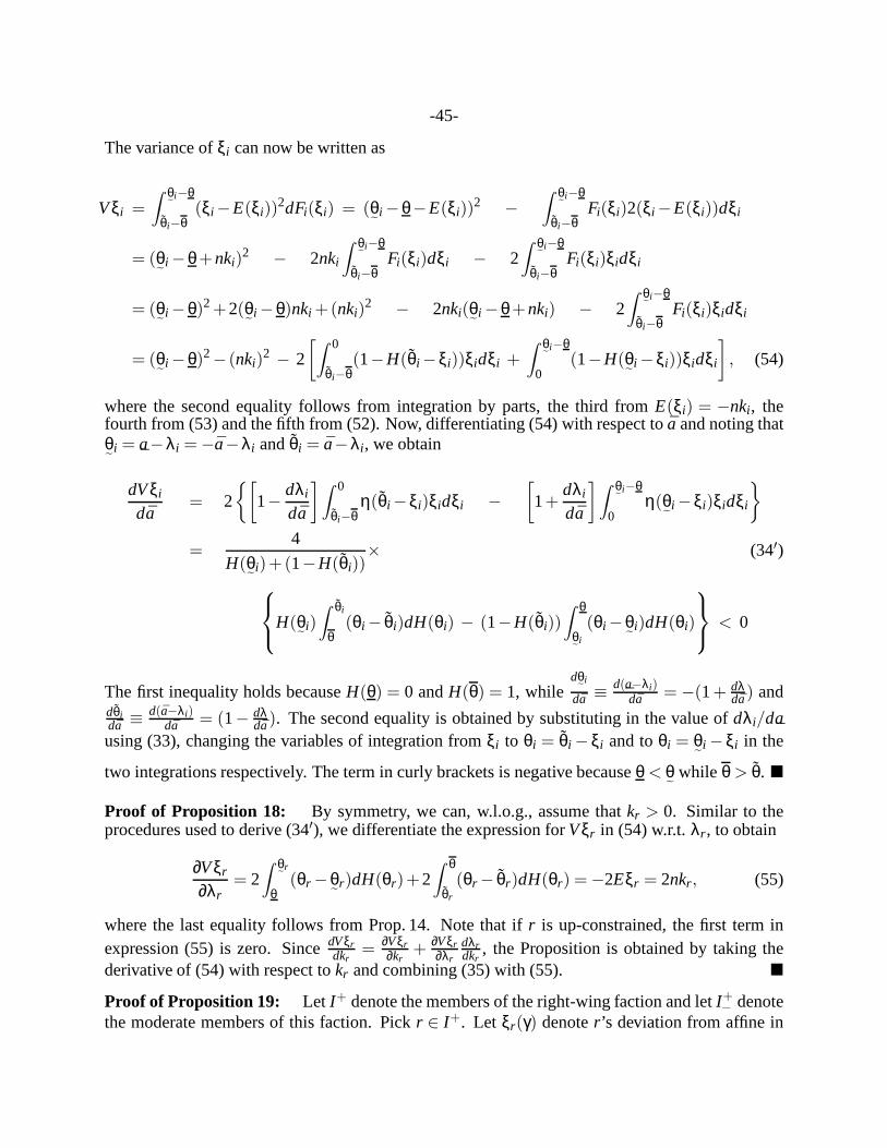
-45-

The variance ofξi can now be written as

Vξi =

∫ θ˜

i−θ

θi−θ(ξi −E(ξi))

2dFi(ξi) = (θ˜

i −θ−E(ξi))2 −

∫ θ˜

i−θ

θi−θFi(ξi)2(ξi −E(ξi))dξi

= (θ˜

i −θ+nki)2 − 2nki

∫ θ˜

i−θ

θi−θFi(ξi)dξi − 2

∫ θ˜

i−θ

θi−θFi(ξi)ξidξi

= (θ˜

i −θ)2+2(θ˜

i −θ)nki +(nki)2 − 2nki(θ

˜i −θ+nki) − 2

∫ θ˜

i−θ

θi−θFi(ξi)ξidξi

= (θ˜

i −θ)2− (nki)2 − 2

[∫ 0

θi−θ(1−H(θi −ξi))ξidξi +

∫ θ˜

i−θ

0(1−H(θ

˜i −ξi))ξidξi

], (54)

where the second equality follows from integration by parts, the third fromE(ξi) = −nki , thefourth from (53) and the fifth from (52). Now, differentiating (54) with respect to ¯a and noting thatθ˜

i = a¯−λi = −a−λi andθi = a−λi , we obtain

dVξi

da= 2

{[1− dλi

da

]∫ 0

θi−θη(θi −ξi)ξidξi −

[1+

dλi

da

]∫ θ˜

i−θ

0η(θ˜

i −ξi)ξidξi

}

=4

H(θ˜

i)+(1−H(θi))× (34′)

H(θ˜

i)∫ θi

θ(θi − θi)dH(θi) − (1−H(θi))

∫ θ

θ˜

i

(θi −θ˜

i)dH(θi)

< 0

The first inequality holds becauseH(θ) = 0 andH(θ) = 1, whiledθ˜

i

da ≡ d(a¯−λi)da = −(1+ dλ

da) anddθida ≡ d(a−λi)

da = (1− dλda). The second equality is obtained by substituting in the value of dλi/da

¯using (33), changing the variables of integration fromξi to θi = θi − ξi and toθi = θ

˜i − ξi in the

two integrations respectively. The term in curly brackets is negative becauseθ < θ˜

while θ > θ. �

Proof of Proposition 18: By symmetry, we can, w.l.o.g., assume thatkr > 0. Similar to theprocedures used to derive (34′), we differentiate the expression forVξr in (54) w.r.t.λr , to obtain

∂Vξr

∂λr= 2

∫ θ˜

r

θ(θr −θ

˜r)dH(θr)+2

∫ θ

θr

(θr − θr)dH(θr) = −2Eξr = 2nkr , (55)

where the last equality follows from Prop. 14. Note that ifr is up-constrained, the first term inexpression (55) is zero. SincedVξr

dkr= ∂Vξr

∂kr+ ∂Vξr

∂λr

dλrdkr

, the Proposition is obtained by taking thederivative of (54) with respect tokr and combining (35) with (55). �

Proof of Proposition 19: Let I+ denote the members of the right-wing faction and letI+− denote

the moderate members of this faction. Pickr ∈ I+. Let ξr(γ) denoter ’s deviation from affine in

-46-

the equilibrium associated with the parameterγ. Sincer is up-bounded, we have

nk+r = −Eξr(0) =

∫ θ

θr

(θr − θr)dH(θr) = 0.5∫ 1

θr

(θr − θr)dθ = (1− θr)2/4

The first equality follows from Prop. 14 and the third from assumption A8(i). Henceθr = 1−2√

nk+r . Moreover,H(θr) = 0.5

∫ θr−1dθ = 1+θr

2 . Now from (36)

dVξr

dkr

∣∣∣∣γ=0

= 2n2k+r

(H(θr)

1−H(θr)

)= 2n2k+

r

(1+ θr

1− θr

)= 2n2k+

r

(1−√

nk+r√

nk+r

)

= 2n(√

nk+r −nk+

r )

Hence d2Vξr

dkr2

∣∣∣γ=0

= n(√

n/√

k+r −2n

)≶ 0 ask+

r ≷ 1/4n. That is, fork′ > k, dVξr(k′)dk >

dVξr(k)dk if

k′ < 1/4n and dVξr(k′)dk < dVξr(k)

dk if k > 1/4n. From Prop. 11, Prop. 14 and symmetry,USW= −2∑i∈I+ Vξi(γ), so that

dUSWdγ

∣∣∣∣γ=0

= −2 ∑i∈I+

dVξi(γ)dγ

∣∣∣∣γ=0

= −2 ∑i∈I+−

αi

(dVξi+n/4(γ)

dki+n/4

∣∣∣∣γ=0

− dVξi(γ)dki

∣∣∣∣γ=0

)

Sincek+i+n/4 > k+

i , we havedUSWdγ

∣∣∣γ=0

> 0 if min(kkk+) > 1/4n and dUSW

dγ

∣∣∣γ=0

< 0 if max(kkk+) <

1/4n. �

Proof of Proposition 20: We first establishλ∗h > 0, so that, from (37),Eξh(λ∗

h) = 0 and thushis the anchor of the game. Suppose instead thatλ∗

h ≤ 0 andλ∗h ∈ int(Λ). (We can easily rule out the

situation whenλ∗h = min(Λ) = a

¯−θ; we omit the details.) Sincekh > kr ∀r 6= h, (22) implies that

Eξh(λ∗h) < Eξr(λ∗

r ) and thusλ∗r < λ∗

h ≤ 0. SinceEξr(λr) = 0 whenλr = 0, (21) andλ∗r < 0 imply

that

λ∗r +Eξr(λ∗

r ) < 0. (56)

From (15′) andλ∗h ∈ int(Λ), λ∗

h = nkh−∑r 6=h(λ∗r + Eξr(λ∗

r )) > 0, where the inequality is due tokh > 0 and (56). This contradicts our supposition thatλ∗

h ≤ 0. Property (37) now ensures thatEξr(λr) = 0, so that single-bounded aggregation games are anchored with anchorh. The secondpart of the proposition now follows from Prop. 12. �

Proof of Proposition 21: Let λλλn denote the MPE of then’th game and letKn = {κ ∈ K :∃i ∈ {1, ...,n} s.t.kn

i = κ andλni ∈ int(Λ)}. From Prop. 20,λn

h ≥ 0 and by construction, the up-per bound on announcements never binds. Hencekn

h ∈ Kn, for all n. Next note that as in theproof of Prop. 4, diameter(Kn) →n 0, so that the limit outcome is a constant function. Sincehis almost-never-constrained, Prop. 9 now implies that the limit outcome coincides with the limitof h’s interim expected CIPO outcomes (which are independent ofθh). Specifically, this limit islimnkn

h +EϑEϑϑϑ−r µ(〈θr ,ϑϑϑ−r〉) = limnknh +Eϑϑ. �