Rational conformal theories from Witten's knot approach: Constraints and their analysis

ANNALS OF PHYSICS 205, 173-205 (1991)

Rational Conformal Theories from Witten’s Knot Approach: Constraints and Their Analysis

PHILIP MURPHY AND SIDDHARTHA SEN

School qf Mathematics, Trinif.v College, Dublin, Ireland

Received December 15. 1989

By studying the interplay between surface diffeomorphisms and the intertwining of N Wilson loops on the Manifold S’ x S’ a set of constraints on the operator content and scaling dimensions of RCFTs is obtained. It is then shown that all constraints obtained for N>4 follow from the N=4 constraints. Two infinite classes of RCFTs, namely the SU(2) affme series and the discrete unitary series are shown to be solutions of these constraints. Explicit expressions for the fusion rule coefficients for both series are obtained. ‘0 1991 Academic

Press, Inc.

1. INTRODUCTION

In a recent paper [ 1 ] we exploited the connection between rational conformal field theories (RCFTs) [2] and knot invariants discovered by Witten [3] to put restrictions on the operator content and scaling behaviour of such theories. Our restrictions included those discovered earlier by Vafa [4]. In this paper we extend our earlier work in several important ways. In order to state our results we first recall a few basic notions. A RCFT may be characterized as a conformally invariant field theory whose physical Hilbert space H splits into a finite sum or irreducible representations of a chiral algebra & = ~~2~0 dR; that is, H = @ ;Hi@ Hi, where dL, LS?~ contain at least the identity operator and the left and right Virasoro algebras. Each space Hi@ Hi is generated by acting first with a primary field 4, (which we take to be self-conjugate) on an X(2) invariant vacuum and then applying the algebra the algebra d to this state. One of the properties of the RCFT is the fusion algebra [S] which labels the possible couplings between primary states; namely,

k (1)

where the fusion coefficients N, are non-negative integers which are to be inter- preted, [S], as the dimension of the Hilbert space associated with a triply punctured surface corresponding to the three primary di, 4,, and qSk. Well-known examples of such theories are provided by the minimal series of Virasoro representations [6], the unitary series [7], and the Wess-Zumino-Witten models [S-l 11.

173 0003-4916/91 $7.50

Copyright 0 1991 by Academic Press, Inc. All rights of reproduction in any form reserved

174 MURPHY AND SEN

We next recall that the connection between knot invariants and RCFT comes from the study of the quantisation problem of a three-dimensional Yang-Mills theory with a pure Chern-Simon action S [12] defined by

S=f-j M

hdA+;AAAnA 1 where k is an integer, A4 a closed compact three-dimensional manifold, A a connection one form of a gauge group G, and the trace is with A in the representation Rj of G. The observables of the theory are taken to be Wilson loops W[Ci, Ri] defined by

W[C,, R,] =Tr,,(PefrdA),

where Ci represents a loop in A4 and P denotes path ordering. The Hilbert spaces obtained by quantising this (2 + 1)-dimensional system are precisely the spaces of conformal blocks of RCFT. We discuss this connection in greater detail in Section 2. Knots enter the problem through the Wilson loops Ci and topology enters, at least at a formal level, because both the action S and the Wilson loop variable WCC,, Ri] are metric independent. It is thus expected that correlation functions of the forms

Z(M, L)=Z(M, W[R,, C,], . . . . W[R,, C,]) = j DAeciSLA1 fi W[C,, R,] j= 1

are topological invariants associated with the link L defined as the collection of non-intersecting but possibly linked knots CI, . . . . C,. Such correiators vanish unless the set of representations R,, . . . . R, consist of integrable representations only [ 13, 143.

By considering the Riemann surface S2 with four punctures corresponding to four primary fields di, dj, dk, and 4, Vafa [4] derived the constraint

1 (N,j,Npk,+N/kpNpil+NkipNpll)hp= (hi+hj+h,+h,)C NqPNpk, module (I), P P

(3)

where hi, h,, hk, h, represent the conformal weights of the primary fields 4;, I$~, &, and br, respectively.

Quite apart from imposing nontrivial constraints on the fusion coefficients NV, and the conformal weights hi, Vafa’s constraints lead to an alternative proof [4] that the conformal weights of RCFTs are rational numbers [15].

Two immediate questions arise. First, what constraints are obtained by considering S2 with an arbitrary number of primary fields present? Second, can one find general classes of solutions of these constraints? We answer both these

RCFTs FROM WITTEN'S KNOT 175

questions using this knot approach. Remarkably, we demonstrate that all constraints corresponding to S* with more than four punctures are derivable from Vafa’s four-point constraint. That this might be the case was realised by Lewellen [16] using a different approach. We then proceed to show that two infinite series of RCFT, namely, the ahine SU(2) [13] and the unitary discrete series [17, 181 satisfy Vafa’s constraints. Taking the modular transformation matrix S which corresponds to the modular transformation z + - l/z as known from the work of Kac and Petersen [ 171, we succeed in summing Verlinde’s formula for the fusion coefficients [S] for both the affine SU(2) and the unitary discrete series. For the afIine series we reproduce the selection rules of Gepner and Witten [13]. On the other hand, although the Kac formula provides the conformal weights h,, for the discrete series [ 171 there was no general expression for the fusion coefficients. We find that the fusion coefficients for the discrete series at level p are given as products of those of two afline models of level p + 1 and p, namely,

N (I,. s,Kq. 3)h. Sk) =N(P+l) +N(P+l)

r,, ‘,, ‘k p+l-r,.r,,u N’P’

P--s,.s,,sk’

The work is organized as follows: In Section 2 we introduce the machinery and key ideas necessary to do calculations in RCFT. In Section 3 we explain the relationship between diffeomorphisms on the Riemann surface and intertwinings of the Wilson loops in the three-dimensional theory. Relations between such intertwinings result in constraints on operators in the Hilbert space of the theory. The simplest is Vafa’s. In Section 4 we present intertwining relations for twists about any number of strands and deduce the resulting constraints for the sphere with many punctures. We demonstrate that all such constraints are contained in Vafa’s four-puncture constraints. In Section 5 we use Verlinde’s theorem to find the fusion coefficients for both the afline and unitary discrete series and deduce that models of both infinite series satisfy Vafa’s constraints. We summarize our results in Section 6.

2. KNOT REDUCTION MACHINERY

Rational conformal field theories appear in Witten’s scheme in the following way. In a quantum field theory with the Chern-Simon action (2) there is no direct way of evaluating the partition function for an arbitrary manifold M. However, if the manifold is of the form C, x S’, where C, is a genus g Riemann surface, the corresponding partition function can be determined in a particularly simple way.

Rational conformal field theories on the plane appear when C, is S*. The calculation of an N-point correlator of primary fields in such a theory requires the choice of N marked points on S ‘. Consider now the manifold S2 x S ’ with N Wilson loops which are unknotted circles of the form {p,} x S’, where pa E S*: a = 1, . . . . N in representations R,. For such a situation a Hamiltonian formalism is appropriate. One constructs the Hilbert space HS2; R,,, ,,,_ R,N on S’ with N marked points bJa= 1, . N. Witten showed that HS2; R,,, . R,N is precisely the physical Hilbert

595/205/l-12

176 MURPHY AND SEN

space of the conformal blocks of a RCFT on the plane with primary fields {q5,} at points { pn}.

Once the Hilbert space is constructed, then one introduces a time direction represented by a unit interval Z= [0, l] and one propagates the vectors in He; R,,. ._., R, on S2 from “time” 0 to “time” 1 (see Fig. I). This operation is trivial, since the C!hern-Simon theory has a vanishing Hamiltonian. Finally, one forms S2 x S’ by gluing together S* x [0] and S* x [l] ; this identifies the initial and final states giving a trace. Thus

Z(s2 X sl; R;,, -., RiN) = TrHs2,,1 ,,., R (1) = dim(ff,z; R,I, R,) (4) ‘N

Observe that the partition function Z(S2 x S’; R, x R,) is a knot invariant, while dimWsz, R,,, . . . . R,N ) expresses a property of RCFTs. Thus the connection between knots and RCFT is explicit. For later use we list a few results from knot theory c31:

Z(S2xS1;Ri)=hio, Z(S2xS’;Ri,Rj)=6, (5)

where R. is the trivial representation. These results depend on an appropriate phase choice (framing) and our assumption that the primary fields are self-conjugate. The fusion coefficients are the dimensions of the Hilbert space with three primary fields:

Z(S2 x S’; Ri, R,, Rk) = dim(H,z: R,, R,, Ri) = N,,. (6)

Thus the fusion coefficients of RCFTs are given by a knot invariant of three unconnected loops in S2 x S’.

Knots in S3 are of particular interest and are described by topological invariants such as the Jones [ 191 and HOMFLY [20] polynomials. These have factorization properties which in the field theory approach of Witten follow from an analysis of the invariants Z(S); L). If these knot theory results are to be put to use in analysing the structure of RCFT it is necessary to construct analogous results for knots in S2 x S’, where the connection between RCFT and knots is explicit. In order to do this we proceed as follows. First we sketch, for completeness Witten’s argument for the factorization property of knots in S3. Then we explain, again for completeness, how results in the manifold S3 may be related to those in S2 x S’.

1

@

2

3

FIG. 1. Wilson loops in .S* x S’ from S2 x [0, l] by identification.

RCFTs FROM WITTEN’S KNOT 177

Once this has been done, obtaining the required factorization or reduction formula for S 2 x S ’ is straightforward.

We start by considering S3 with two links (collections of knots) % and %’ of arbitrary complexity which are linked by a single loop Ri, but are otherwise discon- nected. Factorization is the statement that the knot invariant Z(S’; L(R,, ‘%, ‘93’)) can be expressed in terms of the invariants Z(S3; L(R,, ‘%)) and Z(S3; L(R,, W)). Here and throughout this paper L(R,, X) has the particular meaning that the collection of knots in X are interwoven (linked) by a single loop R,. The formula which we obtain we will call the “cut and join” formula [ 11.

Cut and Join Formula for S3

We begin with a simple configuration. Consider S3 with only the link % present. It is possible to slice S3 into two parts ML, M, such that the exposed boundary on each part is, in fact, S2, possibly punctured at points {P~}~ by severed loops. Let !RR and %, be the knot remnants in 44, and ML, respectively. As we have just discussed, each boundary has assigned to it a finite dimensional Hilbert space

Hs2; %R(P,)' where by %,&J on S2 is meant representations on those elements in !RR which intersect the surface at points {p,}. Note also that the Hilbert space

Hs+-wPo) is canonically dual to Hs2;xLcPaj. The expectation value of Wilson loops in S3 is thus given by a pairing of It/L E Hs~;sLcp,, and $R~ HSZ:Wrcp,j (Fig. 2):

zw; %I = (ICILY ICIR). (7)

Next consider the situation of interest where % and %’ are interwoven by a loop Ri (see Fig. 3). The boundary revealed on cutting M, severing Ri, and leaving %’ in M,, % in MR, is again be chosen to be S*. Take another version of S3 containing a single loop R, and slice this (severing the loop) into B, and B, so that the exposed surface is once more S2 with Hilbert space vectors VIE Hb2; R,, Ri, vR EHs2,Ri, R,. The expectation value of this simple loop is Z(S3; Ri) = (v,; vR). The crucial point to note is that HS2; R,, R, is at most one-dimensional (5) so that $L, t+GR are proportional to vL, vR, respectively. Algebraically we have then

Z(S3;URj, g', ~))Z(s3;Ri)=($'~, $'R)(VL,VR)=($L* VR)(~L, ICIR)

= Z(M,; L(Ri, fl')) Z(MR; L(Ri, s))

= Z(S3; L(R,, W)) Z(S3; L(R,, %)). (8)

FIG. 2. Knot invariant on S2 as a pairing of Hilbert space vectors on S2.

178 MURPHY AND SEN

FIG. 3. Link factorization in S3.

This factorization formula for simply threaded links in S3 we call the cut and join formula. A loop carrying the trivial representation R, is ignorable. Hence two disjoint links in S3 have the particular factorization

Z(S3; w, %) Z(S3) = Z(S3; ‘ix’) Z(S3; !N). (9)

Before we can connect with S2 x S’, another result of Witten exploiting the assign- ment of vectors in Hilbert spaces to boundaries is required.

Toroidal Surgery on S3

Knot invariants in two different spaces may be related in the following way. This time consider S3; L(R,, ‘$3) and remove a solid torus U created by “thickening” the loop carrying R, (see Fig. 4) but not intersecting ‘33. Consider any diffeomorphism K of the solid torus. The resulting torus may be “glued” back to produce a new space M= S3/U u K(U) containing ‘3 and the distorted loop of Ri. However, at the Hilbert space level any such diffeomorphism of the torus surface will have a matrix representation Kti. The basis vectors xi for the Hilbert space of C, had already been

@=@y&

FIG. 4. Geometry of toroidal surgery on S’.


FIG. 5. Basis vector x, arising from Wilson loop in representation Ri parallel to b-homology cycle.

identified by Verlinde [5] as just those arising for U with a single representation Ri circulating within in the sense of a b-homology cycle (see Fig. 5). Consequently, K(xi) = xi K,xj and

Z(a; L(K(R,), g))= ($3 K(Xi))=C K,Z(S3; L(Rj, s1)). (10)

Following Witten we refer to this expression as the surgery equation. Its utility lies in that it relates knot invariants in S3 to those in other compact three-dimensional manifolds. To go from S3 to S2 x S1 we simply need an appropriate map K.

From S3 to S2xS’

We claim that S3/U is also a solid torus so that S3 may always be decomposed into two solid tori (see Fig. 6). Furthermore, the two tori are related to each other by an inversion mapping, taking the common surface of the tori Z, to itself. However, Z, as the boundary of S3/U has the a and b homology cycles reversed with respect to itself as the boundary of U. Thus the inversion acting as a diffeomorphism on C1 is the modular transformation S: z --f -l/z. We observe that this is the case by considering a special situation. Let us regard the three-sphere S3 as being embedded in C*, the space of two complex variables (z,, z2), by the equation

lz,12+ 12212=2. (11)

FIG. 6. Decomposing S3 into two solid tori, one being the complement of the other.

180 MURPHY AND SEN

In C* the flat torus is described by the equations

IZll = 1, lz21 = 1. (12)

This torus divides the three-sphere into two pieces, namely

T+ = ((~1, z&S3 I lzll < l}

T- = ((z,, z2 )ES3 I lz*l< 1). (13)

Clearly,

S3=T+vT-. (14)

We claim that T + and T - are three-dimensional solid tori. The proof is simple. If To is the three-dimensional solid torus,

To= {(zl,zJ~@~I lz,l 6 1, 1~21 = 1).

Then one obtains the homeomorphism (from say) T- -+ To by

(z1,z*)- Zlr3 ( ) 1221

Thus one finds that the representation S3 = T+ u T- of the three-sphere results from gluing together two copies of the solid torus To along the boundary S ’ x S1 with the two factors of the boundary S’ x S’ being exchanged by the gluing; i.e., in the general case if one torus is described by the pair of radii (a, b) the other will have radii (b, a). Such a transformation is equivalent to the diffeomorphism S on the surface of a torus constructed out of two circles of radii a, b as stated above.

On the other hand, if the two solid tori D x S’ and D’ x S’ are glued together pointwise along the boundaries of the discs D and D’ as in Fig. 7, then the manifold

1

gr%

S’

= 00

s'

D x S’ Dx S’ s2x s’

FIG. 7. Construction S2 x S’ from two solid tori.


S* x S ’ is obtained. This geometrical observation is precisely what is needed to put the surgery equation to use relating Z(S3; L(R,, 3)) to Z(S2 x S’; Rj, ‘9I)); i.e.,

(15)

This, at last, is the connection formula. An immediate results is the normalization of the expectation values of simple links in S3 by those in S* x S ’ (5):

Z(S3; L(R;, S,)) = c SikZ(S2 x S’; R,, Rj) = S,. (16) k

Furthermore, as Z(S3; L(R,, R,)) is a topological invariant, it is symmetric in i and j, so that S, is symmetric and for the self-conjugacy here assumed, the unitarity of S, becomes

1 L!$jsjk = 6 , . (17)

That the matrix S, is its own inverse allows passage in either direction between S2 x S1 and S3 with equal ease.

Verlinde’s Formula

Witten’s particular application of these results to RCFTs was to deduce the relationship between the fusion rule coefficients (Nijk) and the matrix elements S, conjectured by Verlinde [S]. As stated above, N, is the dimension of the Hilbert space on S* punctured by Ri, R,, and Rk. Consider S3 with R, threading the otherwise unlinked loops R, and Rk. Employing the factorization formula (8),

z(s3; L(R,, Rj, Rk)) Z(S3; R,J = Z(S3; L(R,, Rj)) Z(S3; L(R,, Rk)).

Applying the connection formula (15) to the first term, the normalization (16) of the last section, and summing over S,, the result is [3] an equivalent form of Verlinde’s conjecture

N, =I siP~skP. P OP

(18)

This equation we refer to as the Verlinde formula. It provides an explicit formula for the fusion coefficients in terms of the matrix elements S, which is useful if the S, are known. This will be exploited in Section 4. For the self-conjugate primary fields, Eq. (18) guarantees that the N,s are completely symmetric.

Reduction Formula for S 2 x S 1

All the techniques necessary to establish a reduction formula for disjoint links in S2 x S’ are now in place. The starting point is S* x S’ with two disjoint links !R

182 MURPHY AND SEN

and ‘$I’. The idea is to change to S3, use the factorization results there (8), then return to S* x S’. To pass to S3, we need the inverse of the connection formula (15) which is found, using the unitarity of S,, to be

Z(S’ x S’; Ri, 32) = 1 SqZ(S3; L(R,, 9l)). i

The formula assumes the presence of a simple loop (R, above). The problem at hand is not possessing such a loop, we invent one. Such a simple path c parallel to the disjoint links may be thought of as carrying the trivial representation R,, thus the inverse connection above gives

Z(S2 X 5”; ‘%, ‘%‘) = 1 S,jZ(S3; L(Rj, ‘%y ‘%‘)),

where the loop R, threads the two links in S3. Now we may use the cut and join formula (8) on the right-hand side with a copy of S3 containing a single simple 1OOP Rj:

Z(S3; L(R,, ‘3, 93’)) Z(S3; Rj) = Z(S3; L(R,, %)) Z(S3; L(R,, ‘Jz’)).

However, Z(S3; R,) = S, (16) which, on combining with the last two equations, gives

Z(S2 X 5”; ‘93, %‘)=C Z(S3; L(Rj, ‘%)) Z(S3; L(Rj, %I)). (19)

Each factor on the right-hand side may be transformed to S2 x S’ through the connection formula (15), resulting in

Z(S2 X IS’; %i, !I?‘)= 1 SjsZ(S’ x S’; R,, 93) Sj,Z(S2 x S’; R,, %‘) j,s,r

=c Z(S2 x S’; R,, 93) Z(S2 x S’; R,, ‘ill’). (20)

We refer to this expression as the reduction formula. It is the S2 x S’ analogue of the S3 disjoint link factorization (9). The expectation value of any two disjoint links in S2 x S’ factorizes as a sum over the products of the individual links with “channels” R,. This result is a key calculation tool in RCFTs, as it translates at once into an expression for the decomposition of traces (4) over the relevant Hilbert spaces. That decomposition will be fully explored in Section 3; in the mean- time (20) i.; quite sufficient to establish that the fusion coefficients, as derived in this knot approach, automatically satisfy duality.

RCFTs FROM WITTJZN’S KNOT 183

Duality and Reduction Formulae for Nlli2, . i,

By duality is meant the property that any four-point correlator may be expanded equivalently over any of the three available channels. In particular, this implies that the dimension of the Hilbert space over the sphere with four-punctures must decompose as

Nijk, = c NijtNrw = c N,,N,,, = 1 N#rw (21) I * r

This is a non-trivial restriction on the fusion coefficients N,. However, we will see that the reduction property of links in S* x S ’ (20) guarantees that fusion coefficients obtained in this scheme satisfy duality. The object under consideration is S’ with four punctures R,, Rj, Rk, and R,. It is clear that for disjoint loops Z(S* x S’; Ri, R,, Rk, R,) is symmetric under interchange of (i, j, k, I) so that in the reduction formula (20) any pair may be taken as !?I and the remainder as 3’.

N,, = diWb R,. R,. Rk, R, )=Z(S*xS’; Ri, R,, Rk, R,)

=c Z(S2 x S’; Ri, Rj, R,) Z(S* x S’; R,, Rk, R,) =I N,,N,,, f ,

=CZ(S2XS’; Rj, Rk, R,) Z(S* X 5”; Rr, Ri, R,) = 1 Nj/vNril , r

=CZ(S*xS’; R,, Ri, R,)Z(S’xS*,R,,Rj, R,)=CNkifNsj,. (22) s s

Duality also implies full symmetry in the indices of N,, (or the symmetry is made explicit by NiJkl= Et NM,Nlk, = & Si~Sj~S~,S/~/S~,, using (18) and the unitarity of S,).

Clearly repeated use of the reduction formula shows that the dimensions of Hilbert spaces on S* with higher numbers of punctures may all be expressed in terms of the fusion coefficients, e.g., with live loops (Ri, Rj, Rk, R,, R,},

Therefore the fusion coefficients defined as the dimensions of the three-punctured sphere determine the dimensions and branching rules of the sphere with an arbitrary number (greater than two) of punctures.

Knot theory thus provides a natural definition for the fusion coefftcients and direct derivations of those properties required in RCFTs. In the next section the geometry of the scheme is exploited; relations between intertwinings of loops in the three-dimensional theory impose constraints on the conformal weights admissible in RCFTs for a given set of fusion coefficients.

184 MURPHYANDSEN

3. SURFACE DIFFEOMORPHISMS AND KNOT INTERTWINING

So far we have considered only the most basic of links in S* x S ‘, namely disjoint, simple loops. One of the most useful facts of knot theory is that any link may be created by braiding sufficiently many strands and identifying end points. In this section the loops of the last section are braided and the effect on CFT is to severely constrain allowable models.

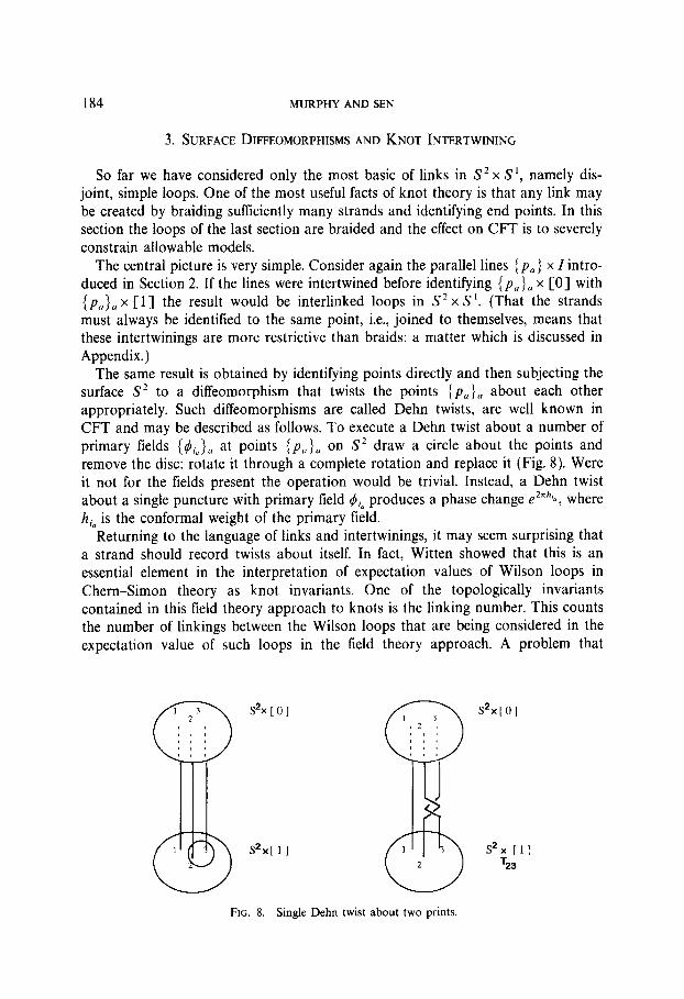
The central picture is very simple. Consider again the parallel lines {pa} x Z introduced in Section 2. If the lines were intertwined before identifying (p,), x [0] with {p,}, x [l] the result would be interlinked loops in S’ x S’. (That the strands must always be identified to the same point, i.e., joined to themselves, means that these intertwinings are more restrictive than braids: a matter which is discussed in Appendix.)

The same result is obtained by identifying points directly and then subjecting the surface S* to a diffeomorphism that twists the points {pU}, about each other appropriately. Such diffeomorphisms are called Dehn twists, are well known in CFT and may be described as follows. To execute a Dehn twist about a number of primary fields {d,}U at points (P~}~ on S* draw a circle about the points and remove the disc: rotate it through a complete rotation and replace it (Fig. 8). Were it not for the fields present the operation would be trivial. Instead, a Dehn twist about a single puncture with primary field 4, produces a phase change e2nhzo, where h, is the conformal weight of the primary field.

Returning to the language of links and intertwinings, it may seem surprising that a strand should record twists about itself. In fact, Witten showed that this is an essential element in the interpretation of expectation values of Wilson loops in Chern-Simon theory as knot invariants. One of the topologically invariants contained in this field theory approach to knots is the linking number. This counts the number of linkings between the Wilson loops that are being considered in the expectation value of such loops in the field theory approach. A problem that

s*x [ 0 ] s*x[o]

s*x [l]

T23

FIG. 8. Single Dehn twist about two prints.


immediately arises is: what happens if two Wilson loops coincide? Or more geometrically how should one count self-linkings of a given knot? Field theory suggests a way of answering this question. Namely, by using a point splitting regularisation method which geometrically corresponds to thinking of a loop as a ribbon. Twisting a ribbon carrying a representation R, through 27r is then a signifi- cant operation and changes the associated knot invariant by the sma phase factor a in = p%.

In general, since the beginning of each strand (p, x [0]) is fixed, the operation of identification followed by Dehn twists about the end (pa x [l]) not only produces the required intertwining of the strands about each other, but twists each strand about itself an integral number of times. On the other hand, as the end result is still a state vector in the same Hilbert space, then every Dehn twist and its effects-both intertwinings and self-twists, is represented by a matrix operator z on the Hilbert space. The intertwinings on n strands forms a group. Each intertwining is represented by a Dehn twist on the Riemann surface, which is in turn represented by an operator on the Hilbert space that encodes both the intertwining and the twisting of the individual strands.

In this work we denote by T the operation of intertwining and strand twisting produced by a given Dehn twist. This allows us to equate the expectation value of the braided loops with the trace of the Hilbert space operator directly; for every such intertwining T of n strands there is a finite dimensional matrix operator z such that

Z(zg X S ‘; T(Rj, 9 Ri,, -., R,)) = Z(Cg X T 1; R, 3 Ri2, -.t R,) = TrHLg.R,,,R,2, ,R, (T). (24) n

This is more than just an elegant statement. Intertwinings are very close to braids and various defining relations exist between braid elements. It is already clear from CFT that the transformation properties of primary fields subjected to Dehn twists are explicitly dependent on the actual conformal weights. It will be seen shortly that the simple topology of S2 combined with the power of the reduction formula of the last section will determine the r matrix elements sufficiently well for intertwining relations to impose constraints on the conformal weights of the theory.

The first step is to determine the matrices involved. From the earlier discussion, twists about a single strand T, are represented by a phase times the unit matrix on the Hilbert space:

Tr HS2,R,,R(~i) = Z(S2 x S’; Ti(Ri, ‘3)) = CC,Z(S~ x S’; Ri, %) = txi dim(H,j,%, %). (25)

Next consider the intertwining of two loops Ri and R, created by a Dehn twist about punctures p1 and p2 on the Riemann surface. We emphasize that the effect of the twist is to both wrap the strands about each other and twist each about itself. The first non-trivial example arises on S2; Rj, Rj, R,. Inspection of the topology of the sphere (see Fig. 9) shows that the twist about the first two punctures is

186 MURPHY AND SEN

1 2

6 3

- -

FIG. 9. Topological identity for intertwinings on S2 with three strands.

indistinguishable from a Dehn twist about the remaining puncture pX. The corresponding Hilbert space operators must then be equal, i.e., tV = zk so that

This topological argument concerning Dehn twists on the sphere is completely general and will be used throughout this work. Only on S* with 3-punctures is riJ diagonal.

Contrast this to the form of tii on S* with four punctures (corresponding say, to loops Ri, R,, Rk, and R,). Topology is of no use as it simply equates rii= rk,. Instead, we note again that the intertwining created by the Dehn twist about {pi, p2} has no effect on the Ri, R, loops, so the reduction formula (20) may be profitably employed to separate the affected loops:

Z(S2xS1; T&R,, R,), Rk, RI)=JZ(S2xS1; R,, T,(R,, Rj))Z(S2xS1;R,, Rk, R,).

The first factor on the right-hand side is the expectation value for two intertwined loops with just three present in all: from (26) it is OI,N~,, while the second is just the fusion coefficient,

Tr Hr2:R,.n,.q.n,(~ii)=Z(S2x s’; Tv(Ri, Rj, Rk, R,))=C ~tNt~Ntk/. ,

(27)

With four punctures zii is no longer acts by a phase but the reduction formula serves to factorize the Hilbert space into those over 3-punctured spheres, where it does act diagonally.

Indeed for any intertwining that factors over loops, T(Yl, %‘) = TA( ‘ill) T,(%‘), it


then follows from the reduction formula (20) that traces over the corresponding Hilbert space operators 7, tA, and tg, are related as

Tr HS2;s,R.(7) = 1 TrHS2.R,.J7A) TrHS2.RJ%J. I

(28)

This Hilbert space trace factorization, a consequence of the properties of links in S2 x S’, is the key to determining the operator matrices corresponding to twists about arbitrary numbers of strands. Indeed, with 7 the unit matrix, this is the result behind the duality and dimension reduction expressions of the last section.

The last non-trivial possibility with four strands is to twist the strands about each other three at a time. Once more, the topology of S2 shows that such an intertwining is indistinguishable from a twist about the remaining strand, or on the Hiibert space: ziik = tl.

However, closely connected to the commutator relation of adjacent braiding operators on the sphere (see Appendix) is the first intertwining relation,

T, Ti T, Tk = T, Tjk Tki . (29)

In essence, wrapping three braids about each other may be achieved by rotating all about each other at once, or by twisting each about the other, two at a time. In the first case, involving a single Dehn twist, the strands are each self-twisted once, while in the second, each is involved in two Dehn twists and so end up self-twisted twice. As the Ts must encode this twisting, a self-twist of each strand is added to the left- hand side in (29). (The clearest way to see this and future identities is to construct a three-dimensional model.) On using the topological result specific to S2 with 3-punctures, riik = T, , this intertwining relation becomes an identity between Hilbert space operators,

7ij7,‘k7ki= Tit,TkTijk = TiTjitkt,. (30)

This identity was first introduced in the context of CFT by Vafa [21], starting from an entirely different viewpoint, and who then [4] put it to the same use as we are doing.

The right-hand side is known completely from (25) to be the product of the phases CL$/XkC1, times the Nykl unit matrix. While the order of the double twists on the left-hand side of (30) allows for cyclic permutations, the operators do not commute. Worse, the trace of their product cannot be factorized by the Hilbert trace reduction formula (28). However, being finite dimensional matrices, the logarithm of the operators, In 7 is well defined and, using the usual identity Tr In = In Det, the traces of logarithms of products separate as a sum. Taking the trace of the logarithms of the binary intertwinings in (30) one obtains

Tr HsZ:R,,R,,Rk,R,(ln(71i7jk 7ki))

=Tr Hs~,R,.R/.R~,R~(~~(‘~~)) + TrHS*,R,,Ri.RI,Rl(1n(7jk)) + TrHsz,,,,,,k,,,(1n(7k,)).

188 MURPHY AND SEN

Furthermore, ln(z,) still acts as the identity with respect to Rk, R,, so its trace may be reduced as (28)

where the arguments preceding (27) were used in deriving the last expression and i 2rchp = ln(cr,). Taking the trace of the logarithm of both sides of the operator identity (30), Vafa’s constraint (3) results in

CNiikLphp=Nijk[(hi+hj+hk+hl) module(l), (32)

where by Niikr,p we have defined

NV/c, p = Ngp Npkl+ Njkp Npil f Nkip Npj/

or, equivalently, as it was first written by Vafa [4],

n a?~ = (aiajaka,)Nyk’. P

(33)

For a given set of fusion rules, (3) is a knot-induced four-point constraint on the values of the conformal weights of the primary fields involved. In terms of the three- dimensional Chern-Simons theory, it is a constraint between the highest weights of integrable representations and the occurrence of certain invariants in the reduction of direct products of those representations.

Examples

The particular class of Chern-Simons theories that Witten treated in most detail were the integrable representations of level K of the afline Lie algebra SU(2). There are K+ 1 highest weights at each level and the fusion rules for arbitrary K are well known [ 133. In Section 5 we will show that the four-point constraint above is satisfied for all levels of K. For the purpose of example we choose K = 2, for which the fusion rules for the fields (d,, &, &} (4, is always the identity operator with conformal weight h, = 0) are

The reader will recognize that this theory has the same fusion rules as the Ising model. This is the first member of the unitary discrete series, and the connection


between that series and the Chern-Simon+based results obtained here so far will also be discussed in Section 5.

A few general comments greatly simplify the evaluation of the possible N4 (where N is the number of integrable representations) constraints in (30). For all unitary, self-conjugate theories, N,, = 6, (recall (5)) with the result that they need not be listed. Furthermore, setting I = 1 in the 4-point constraint (30), it collapses to an identity. And, since the constituents of the 4-point dimensions N,, = 1, N, Npk, are all positive (being themselves dimensions), then if N,, vanishes so do Niikr,p by duality. Hence the only constraints in (30) occur for N,, # 0 and none of the fields is the identity.

For the model under consideration this leaves but three combinations of four primary fields, which we indicate in the first column:

d2424242 (a;)* = a;

4242d343 (a;xy = ct; (35)

$3434343 (Q = 1.

The three equations admit the following set of solutions:

h,=O, 2 - h =2m+1 h =2n+1 16’ 3 2’

The actual weights for the afline model are (0, A, $), and (0, &, $) for the Ising model. Thus it is seen that a set of conformal weights satisfying Vafa’s four-point identity for a given set of fusion coefficients is not unique.

Vafa was the first to obtain these types of solutions. In fact, he used (3) to show that the conformal weights of theories whose Hilbert spaces are finite dimensional must be rational [4]. That the constraints are non-trivial is clear. Intertwinings about one, two and three strands together have been examined. But with more strands there will be new intertwining relations and new constraint equations. Take, for example, the sphere with five punctures. The novel features are twists about four strands at a time. These four strand intertwinings may be factored as

T,,, T, T, Tk T: = T,, Tjl T,, Tok . (36)

Again, there is a simple intuitive way of understanding this. If the first three strands are intertwined then intertwining a fourth strand about each of the first three in turn, will leave all four correctly intertwined, but each of the original three strands will have been twisted twice, while the forth was involved in three twists. Taking into account the twist all strands receive from the twist about all four together, the individual self-twist terms in (36) are seen to balance both sides.

In terms of the Hilbert space operators, the topology of S* with five-punctures implies that riikr= z,, while tiik may be read off from the first equality in (30) (the

190 MURPHY AND SEN

second, dependent on the topology of the four punctured sphere is no longer valid), so the final form of the identity is

(tilZjlZkl)(ZijZ,k~ki) = z,(z;)2(tj)2(zk)2(zr)2. (37)

This matrix identity was introduced in [ 11. Note that it is not symmetric in indices, so the order in which fields are chosen must be taken into account. Double and self- intertwinings are evaluated as in the derivation of (33) to give

where N,,, p now involves six terms corresponding to the various double intertwinings,

N,,tn, p - - Nilp Npjkm + Nj/p Npikm + Nk,p Npi/m + NgpNpk/m + Njkp Npilrn + Nkip Np,/m

and N,, is given by (23). There are four new constraints at the five-point level for the affine K = 2 example

above:

4242424243 ((a;)‘~~)~ = a:

434242d242 ((a3a:)2a2)2 = aza:

42d2fP34343 ((aza:)2a3)’ = ct:a3 (39)

d13#3&#24& ((aia2)2a2)1 = a:.

For this example, the solutions to the four-point constraint (33) are consistent with the above live-point constraints. This leads to the question: do constraints derived from higher numbers of punctures ever provide additional information to that encoded in (33)? Indeed, is it possible to prove that solutions to the four-point constraints are even compatible with those from higher numbers? In the next section we show that, in fact, all higher constraints are just identities involving (33).

4. INTERTWININGS OF MORE THAN FOUR STRANDS

In this section we show that constraints arising on the sphere with with more than four punctures are derivable from the 4-puncture constraints (3). The proof is inductive: we describe the identities between operators of the Hilbert space over the sphere with N punctures: we show that the identities on the sphere with N + 1 punctures are true if they are true for N punctures: we have already established them for N=4.

First we show that the intertwining of an arbitrary number of strands may be written in terms of a succession of double Dehn twists, with a given simple iterative procedure. With N strands intertwinings of p at a time for 1 < p < N - 1 constitute


all the basic operations. To see that all such intertwining relations give rise to Hilbert space identities with the same content as the 4-point case, it then s&ices to show this for the iterative step itself and the first non-trivial case, i.e., that with three strands. That iterative step comes easy as it is the generalization of a comment made in Section 3, relating intertwinings about p strands to those about p - 1:

(40)

The intuitive picture is that the first one intertwines p - 1 strands at a time and then the pth, with each in turn, and finally the balance for self-twists. Iterating the sequence to the initial double Dehn twist, one obtains the following intertwining relation on p strands:

Ti,i~...i~(Ti,T;,-.-Ti~~,Ti~)P~Z

= (Ti,ipT;21p “‘Ti,~ITi~)(TiliP~LTjZip-I .. Ti,,-z+l) .‘. (TiliZ).

These relations are reflected in identities between Hilbert space operators. For the purposes of clarity, we indicate that a matrix operator T exists on the Hilbert space over S2 with N punctures by rCN) (though we leave the identity of the reprsenta- tions present at the punctures to the context). The intertwining of p strands will have different matrix representations for all N> p + 1. All the information in (41) is compressed into the iterative identity

providing the three-strand identity holds:

(42)

(43)

In addition, all the identities due to the topology of the sphere with N-punctures must hold, i.e., for 1 d p < N - 1,

(44)

We do not in fact deduce the above identities from the four point, but we demonstrate that, at the level of traces of the logarithm, the constraints on the conformal weights encoded in them do not further restrict those obtained at the four-strand level (33). The general strategy is a deductive iteration on top of an iteration: we assume all the above iterative identities (42), (43), and (44) hold for N strands and then show they must hold for N + 1 strands. Given that they do for four-strands (30), the proof is then complete.

Notation. It is clear from equations such as (27) that labels for Hilbert spaces are becoming cumbersome and will be unmanageable as the number of punctures increases. As the rest of this work involves only genus zero Riemann surface S*, we denote the Hilbert space arising on S2 punctured by loops Ri, R,, . . . . R, by

Ha: R,, R,, . R, E Hi.,, . n. (45)

595:205!1-13

192 MURPHY AND SEN

We start with the simplest of the three elements, namely that (44) arising from the topology of the sphere with N+ 1 punctures; providing that p > 1, then the Hilbert reduction formula (28) allows the decomposition of the (N+ l)-strand operators to components on fewer strands:

The topology of the sphere with p + 1 punctures implies that a Dehn twist about p-punctures is equivalent to twisting about the remaining puncture alone,

T~H,,,~ ,,(~&+..‘.!,)=Tr, 11’2 ‘++I (Z!P+1’)=Ni,i2...;i7,a,

The trace of a twist about p-punctures on a Hilbert space over S2 with N+ 1 punctures is thus

(47)

Because any twist is expressible directly in terms of the conformal weights CI,, identifies (44) and (42) are not merely formal statements. However, if two operators do not commute, different unitary transformations are necessary to effect the diagonalization. As emphasized by Vafa, taking only the (logarithm) of the determinants ( = Trace In) of products eliminates those unknown matrices. The diagonalization (47) is symmetric in that

Tr “w iN+, (t~~2~.!~)=~N;liz...ip~a~N~;,+,ip+Z...~N+,=TrH,,,2 ,N+,(z~~~~i~~2,,,iN+,); (48)

this is the topological operator identity (44) at the level of logarithms and traces. If p = 1 then (44) defines the action of twisting N strands. The method employed in this simple derivation is used throughout: use the reduction formula to decompose N+ 1 strand operators into ones defined on a smaller number of strands, where the desired relations are assumed.

If the number of twists is less than N, the inductive result follows directly, i.e., P -c N,

In particular, the four-puncture identity (43) must hold for N + 1 punctures.


Not unexpectedly, it is only twists of N strands on the (N+ l)-punctured sphere that hold out the possibility of new constraints. And these we now show are nothing but reformulations of constraints from fewer strands. In this particular case we have the topological identifications (44)

zy’,) = zy+; l) and T y. +i’,‘_ , = 7 ;;.;+y

so that the iterative constraint (the trace of the logarithm of the identity (42)) we must derive becomes

Th, ,N+,[ln(z~~+ ‘)zif”+ l). . . (zj:+ 1))N-2ziNN+ “1

=Tr H,, ,,+,[ln(~j~~““‘t~~-~,:‘~j~.+~~+,)l. (50)

We begin the left-hand side. The reduction formula introduces an extra loop R, in both factors so we separate two loops Ri,, R, from the others. With the identity (50) on N punctures in mind, we factorize the product of self-twists as

The factors separate under Tr In, the first one now involving only N- 1 strands and may be decomposed using (28) into

The expression in the trace is ripe for (50) but missing a factor z:~‘, the trace of whose logarithm may be added and subtracted:

Writing the various twists involving the r-strand in terms of as (47) and resuming over r (see (23)) the expression in terms of the operators on N+ 1 strands becomes

Tr H ,,.. ,N+,Cln(r~~~l)...zinr-liv (N+l)~~~~+l,)) T~:~+Y))] -Tr,,. .,,+,[ln(zj~~l))]. (52)

The second factor in the original product (51) is evaluated in a similar manner. This time in order to exploit the four-puncture identity (43), the three self-twists already present are augmented by the missing fourth by adding and subtracting traces, resulting in

Tr H,, ,N+,[ln(7~~+1)Z~~+ ‘)zi:+ “)I

=Tr H,, 2N+l[1n(ti~iN (N+l)T!N+l) (N+1)Z(N.+l))_ln(zl~2~~“)].

q-24~~ ‘ili2 we+ I (53)

Adding the two contributions (52) and (53) results in the desired result (right-hand side of (50)). Therefore any set of conformal weights that satisfy the intertwinig

194 MURPHY AND SEN

constraints (3) for the sphere with four-punctures will satisfy any identity arising from the sphere with more than four punctures. This constraint (50) arising from the twisting of N strands on the N+ 1 punctured sphere is exactly that considered by Lewellen [ 16, Eq. (3.13)] by considering the monodromy properties of confor- ma1 blocks. He also realized that it could be obtained from the four-point constraints. Readers familiar with the permutation braid group on the sphere will have found much of the demonstration above familiar. In the Appendix we investigate the relationship between the Hilbert space operators corresponding to intertwinings that have naturally arisen from Witten’s knot interpretation of CFT and the permutation braid group with monodromy on the sphere.

5. AFFINE W(2) AND UNITARY DISCRETE SERIES

Having established the uniqueness of the four-point constraint, we now demonstrate that two infinite series of RCFTs, the afline SU(2) algebras of level K and the unitary discrete series are indeed solutions to Vafa’s four-point constraint. While the Kac formula [17] provides the conformal weights of the discrete series, there was no general formula for the fusion coefficients. We find such an expression starting from the known inversion matrix elements S, [ 181 and using the Verlinde formula (18). We will show that the fusion rules of the discrete series models are closely related to products of those from the affine series. We start then by deriving the (already known) fusion rules for the afline series of level K and demonstrating that together with the conformal weights they satisfy the four-point constraint for all K.

Affine W(2) Series

The conformal weights and S, matrices are [ 13, 171:

i*-1 hi=-..---

4(K+2)’ S,=gsin (s), i= 1, . . . . K+ 1. (54)

Note that the representation index now runs from 1 to K+ 1, so that the trivial representation is now labelled by 1. Verlinde’s formula (18) then gives the fusion coefficients as

K+ l NW-=(&) ,Fb (

sin(ti0,) sin(tjBK) sin(M,) sin( to,) > ’ (55)

where OK = n/(K + 2). N, is to be the dimension of a Hilbert space but that (55) produces an integer at all is not obvious. We break it down to a sum of simpler objects. Define the integral function

L ~ ’ sin( Ntn/L) Mf;= c r=l WWL) .

(56)


The fusion coeflicients are readily rewritten in terms of this as

N, = & {MiK,:.‘k+MkK=j7_j+MkK=iZ_j--MiK+fi:k}.

The amazing part, which makes progress very smooth, is that Mf; has a simple form. In what follows we mean by 6fd a function which takes the value 1 if N is odd, 0 otherwise.

ML,=c?$~(L-NI~~); (58)

i.e., for N even, the function vanishes and, for only the mod 2L value of N, (NIZL) appears. This expression is straightforward to establish by using trigonometrical formulae up to L = 5, but a general proof is provided in [22], which we sketch below.

Noting that sin (Ntn/L) = sin(fltrr/L), where fi= N 1 ZL, the value of N modulo 2L, it is clear that

sin(Ntrc/L) eRrai’L-~-Wrni’L sin(t~,L) = emilL _ e - mi/L = e

-(fi+l,Ci,n,Lj ’ Zr(rZni/ZL) Ce .

r=l

Using the symmetry t + --t in the definition of Mf;, it is straightforward to see that

The key element in [22] is the well-known trigonometric identity in number theory [23], where for N and P integers,

Inspection of the right-hand side of (59) in light of this (and noting that 0 < fi< 2L) leads directly to the desired formula (58).

The expression for the fusion coefficients then becomes

NVk=qK+2) dpf?+k (2(K+2)+(i+j+k)J,,

Assuming i + j+ k is odd, the result will be unity if the terms in parentheses have their usual value. On the other hand, if any of the last three become negative, or the second exceeds 2L the modular evaluation of the terms introduces a deficit of 2(K+ 2) which causes the entire expression to vanish. (As k < K+ 1 these latter two conditions are mutually exclusive.) For given values of i and j, N, will vanish if k

196 MURPHY AND SEN

is either too large or too small-it acts as a “gate” function excluding every second integer. Thus, for given i and j;,

{

0 if Ii-j1 ak

N,=S;pj+k 1 if [i-j1 + 1 ik<min(i+j- 1,2(K+2)-(i+j)- 1) (62 1 0 if k>min(i+j, 2(K+2)-(i+j)).

Possibly the clearest way to express the information in (61) is in terms of the fusion algebra (1) to employ the original formalism of the fusion rules, where for a given value of i, j

min(i+j-1,2(K+2)-(i+j)-1)

diXQli=CNgkdk= c G!;,k4k, (63) k k=li-jlfl

The first upper bound comes from the third term in (61), the second upper bound from the second term. The various l’s appear as i+ j+ k is odd. These are the selection rules in [13, 171. Starting from the inversion matrix S, which come directly from the Lie algebra, we have calculated the selection rules for the associated integrable representations.

Examples

That the afftne models are self-conjugate follows from the explicit form of the aftine fusion rules (63):

$1 x $i = #i, i=l , *.., K+ 1,

so again there is no need to record the values of the fusion coeffkients involving the trivial primary fields. For the use in the next section we record the fusion rules for K = 1,2, 3. The only non-trivial rule for the Gaussian model K = 1 is #2 x d2 = $I. The fusion rules for K= 2 were presented in the example used to illustrate Vafa’s identity (34). For K = 3, the fusion rules are

42X42=4I+h? 42xd3=42+44, $2xd4=43

hxh=h+h* 43x44=42 (46)

44X44=41.

ASfine series and the four-point constraint. To investigate the four-point constraint (3) we need both the four-point fusion coeffkient N,, and the numbers N,,,,,. The four-point coefficients are obtained by summing the fusion rules over all channels (22). But as N, act as gate functions for given i, j, the product of two such functions is another given by their overlap (if any),

I> -1 Ngcr=~Nii,N,,,= 1 sg~~.+.6~d+dk+l=8~V:9+k+10(r, -r<)(r> -r<)h (65)

7 I< +1


where r, is one greater than the common lowest bound, i.e.,

r,=min{i+j,2(K+2)-(i+j),k+I,2(K+2)-(k+I)}

and r< is one greater than the common lowest bound i.e.,

r< =max{(j-iI, I/-kl}.

The theta-function records that the four-point coefficient vanishes if there is no overlap at all. We calculate the left-hand side of the four-point constraint using the conformal weights in (54) and summing over the same overlap region as above:

~Kjurhr=$$$( 1 (r,r<)+W&,- 1) 3 perms

The permutations are those in the three terms that comprise the left-hand side, {ijk} + {kij} + {jki}. From the form of r,, the calculation may be divided into two general cases depending on whether i + j + k + I is greater or less than 2(K + 2). As Cr Nijur is symmetric in {i, j, k, I} from its definition, as is the division just proposed, it suffices to consider any general ordering i < j 6 k 6 I and, in order that all maxima and minima are uniquely resolved, k + j< i + 1. For the case i+j+k+1<2(K+2),

1 (r,r,) 3 perms

=max(li-jl, IkkII)min(i+j,2(K+2)-(i+j),k+Z,2(K+2)-(k+Z))

+max(lk-iI, Ij-rl)min(k+i,2(K+2)-(k+i), j+Z,2(K+2)-(j+Z))

+max(lj-kl, Ii-/I)min(j+k,2(K+2)-(j+k),i+Z,2(K+2)-(i+Z))

=2((1-k)(i+j)+(Ik-ij)). (67)

On the other hand, for this ordering,

2N,,=r,-r,=i+j+k-1 (for any permutation),

which finally gives (bearing in mind the form of the conformal weights)

1 N,,,A = I

&(i2+j2+k2+12-4)=Nok,(hi+h,+h,+h,).

That the equality is exact is fortuitous as will be seen immediately as we consider the other possibility, namely, i + j + k + I> 2(K+ 2). The only difference is that the upper limits are of the form 2(K+ 2) - (k + I) etc., so that

xN,,,,h,=Nv,,(h,+hj+h,+h,)-N,,, (i+j+k+:-2(K-2)). (68) r

198 MURPHY AND SEN

Since N,, vanishes unless i + j + k + I is even, the extraneous term is always an integer, vanishing mod( 1). For example, consider the four-point &#2#4d4 for the K = 3 model described above. On the one hand,

ZN,,,.h,=Z(6,,+26,~)h~=o+2$, i-

while on the other,

The excess of 1 being that predicted in (68). Thus all level K aftine SU(2) models satisfy the four-point monodromy constraint

(3). In the same manner we tackle the more complex case of the unitary discrete series.

Unitary Discrete Series

Recently [24] it has been shown that the unitary discrete series is also equivalent to a series of three-dimensional Chern-Simons theories. Thus all our conclusions regarding constraints are applicable. We start by using Verlinde formula to calculate the fusion coefficients. The conformal weights of the unitary discrete series are given by the Kac formula [17]. Each level p model is parametrized by two integers r, s, for which the conformal weights are

h =(rP-s(p+ l))‘- 1 rs

4P(P$l) ’ l<r<p+l-l,l<s<p-1. (69)

The formula has the important symmetry h,, 1 _ r,p--s = h,,, so that the number of primary fields at each level p is p(p - 1)/2 and are singly counted by imposing the inequality pr < s(p + 1). The inversion matrices for this system are [ 17, 181

s, = r 4p(p8+ 1) (-l)(‘lfSl’(q+*)sin (5) sin(y), i= (r,, s,), etc. (70)

The fusion coefficients are to be calculated from Verlinde’s formula (18),

N, = 8

4P(P+ 1)

X ( sin(rir,8,+ i) sin(r,r,0,+ ,) sin(r,r,Q,+ ,) sin(sis,O,) sin(s,s,e,) sin(sks,O,) sin(r,8,+ r) sin(s,0,) )>

(71)

where d = (ri + si + r, + sj + rk + Sk) and 8, = 71/p, etc. The sums over s, and r, are symmetric under r, -+p + 1 - r, and s, +p - sI, so that the sum may be extended


over the full range of Y, and S, at the coset of a factor of 2. The summations are then separate, apart from the phase factor A. Inspection of the expression for the afhne fusion coefficients (55) shows that, if A is even, the fusion coefficient of the discrete series factors as the product of those for two afhne models of levels p + 1, and p:

N, = N(P+‘)NP r, ‘, 4 .S~S,S~ 3 A even.

Warning. We denote the fusion coefficient of afline “level” L and representations i, j, k as N$‘. This L E K+ 2 in the notation of the last section.

If A is odd, the extra phase may be absorbed by setting ri + p + 1 - ri and si -+ p - si in each sum (as NFL ;. L ~ j.k = N1.5: lir there is nothing preferential in the choice of i):

Moreover, as the afIine fusion coefficients vanish unless the sum of their arguments is odd, one of the last two expressions must always vanish and the fusion rules for the unitary discrete series are expressed concisely as

where (for completeness), from the last section (62)

N;!$ = ij odd. 1 if Ii-j1 + 1 <k<min(i+j-- 1,2p-(i+j)- 1) r+Jfk 0 otherwise.

This is a most useful result which comes directly from the properties of knot invariants by way of the proof of Verhnde’s conjecture. Just why each level p discrete model should be so closely related to the two afline models of levels p + 1 and p is not obvious to us. The fusion rules are given by an even simpler formula, as the symmetry inherent in the parametrization of the fields allows for the second term to be recorded in the first if the summation over the primary fields is unrestricted :

= c r,qrk &S/Sk rkSk’ N(P+ 1)N’P) 4

rk. Sk (73)

The self conjugacy of the discrete series is then assured by that of the ahine:

Using this formula to determine the fusion rules for any model in the discrete series is straightforward. We consider a few examples.

200 MURPHY AND SEN

Examples

The well-known fusion rules of the Ising model (p = 3) emerge as follows: since h2,* = & and hl,* = &, we tentatively identify (T = & and $ = d,,2. The two afline models involved are, (72), K = 1 and K = 2, whose fusion rules are given in (64) and (34), respectively :

The second example is a Potts model, p = 4. We label the primary fields in order of increasing conformal weight:

The N(2), afline models involved are of levels 4 and 5 (K= 2, 3), whose fusion rules were presented in (34) and (64), respectively. Using (73), the fusion algebra for the Potts model are then

*zxtiz=z+*3+*5+*6 tizx*3=*2+Ic14 $*xti4=IcI3+$5

*2x*5=*2+*4 $*X1//6=*2 ti3x+3=z+IcI5

*3X$4=*2 $3xti5=$3++6 *3x*6=*5 (75)

11/4xti4=z+Ic/e *4x*5=*2 *4X*6=*4

*sx*s=z+*5 $5X*6=*3 *6x*6=I.

Discrete Series and Vafa’s Constraint

Taking advantage of the symmetry over summations (as in writing the fusion algebra (73) the dimension of the Hilbert space on S2 with four-punctures is

&,=I NijrNrk,=N~~,1~,r,N~~,,,I,,,+NjP++~1)~,,r,,r~,,,N(P’ P--s,,~,,sk,sl’ (76) f

The first term has the phase (in analog to A in (71)) A4 = ri + rj + rk + r, + si + sj + sk + s, even, the second odd, and once more the vanishing of the afftne four-point coefficients guarantee that the terms are mutually exclusive. (One would be forgiven for suspecting the second term to be an artifact as it vanishes for the Ising model

RCFTsFROM WITTEN'S KNOT 201

with the primary fields 4,.,, pr < (p + 1)s that we chose. However, even with that ordering, the $2$2$2$4 Hilbert space of the Potts model has (75) dimension

N ‘,h$2$2$4 = N(2,2)t2,2,(2,2)(2, 1) = N:::, Nr2i2 + Ny2;, N$;i2 = 2,

with the first term vanishing.) The term in Vafa’s constraint describing twists about the three pairs of strands

(3) also has two contributing terms,

Reiterating, the two contributions (A4 odd and even, respectively) appearing in each of the last two equations are mutually exclusive and the constraint must be satisfied for each case separately. Were the conformal weights of the discrete series to separate cleanly between the two affme models, the proof would be complete. As it is, they almost do:

h Jrd-s,(p+ l))‘- 1 1-rs f

4P(P+ 1) =phy+“+(p+ l)hjp’+ -+ .

( ) (77)

The last term is a minor problem. Combining these last two equations and using the Vafa constraint for the alline models, the (possibly) non-integer remainder is given by, for d even,

R A even = 1 N~,Nt~ht - N,,(hi + hj + h/c + h/l

=i( 1 (~)(~)+Nbi(ri~i+r,~I+I**+ri~,-l)), (78) 3 perms

where <r>ii = C, N,,,,,, (pfl)N$filt)rt and likewise for s,. But these sums are easy to carry out, giving, for example,

Keeping in mind that the afIine four-point functions vanish unless the sum of the arguments is even, a little work shows that Rdeven is indeed an integer. Exactly the same holds for the other terms (d odd) and the constraint is met.

6. CONCLUSIONS

In this paper we have shown how ideas from knot theory may be used to tackle the problem of classifying RCFTs. That knot theory is relevant to this problem is clear. Even alternative approaches to the classification problem [4-6, 10, 16, 281,

202 MURPHY AND SEN

using, for instance, quantum groups [26,27], are known to be intimately connected to ideas involving braids and knots. This connection now so explicit is, nevertheless, quite remarkable.

In this paper we have systematically studied the constraints placed on RCFTs due to the interplay between surface diffeomorphisms and the intertwining of Wilson loops. Using Witten’s knot approach we had previously [ 1 ] obtained Vafa’s four-point constraint. In the knot framework, the heart of that constraint is the intertwining of four Wilson loops induced by Dehn twists on the sphere with four primary fields. Subjecting S2 at t = 1 to a Dehn twist will braid the hitherto parallel Wilson strands. However, the path-integral nature of the (Chern-Simon) theory again implies that there will be an induced action on vectors in the Hilbert space. Consequently, any relations between the generators of intertwinings in the three- dimensional theory are translated into identities between Hilbert space operators.

In this work we have clarified that derivation and shown how knot factorization properties in S2 x S’ give rise to precisely the factorization of traces over the Hilbert space that recover the results of Vafa [4]. If T is an intertwining of n strands, Ri, , . . . . R, that factors as

T(Rij 7 ...y R,) = TAR,,, . . . . Rip) T&p+,, . . . . R,),

and z, rA, 7B the corresponding Hilbert space operators on n, p, n - p strands, respectively, then the knot factorization in S2 x S’ determines the Hilbert space trace factorization

Tr HA-=. R,, R+, (‘1 = 1 TrW~~,.~ ,,,.., R (‘A) TrH~2;~,.~p+ ,,,,,, ,tn(7B). r ‘r (79)

By considering all possible intertwining generator relations, this trace factorization formula enables us to determine a complete set of constraints on RCFTs on the sphere with an arbitrary number of primary fields. We demonstrated that all constraints pertaining to S2 with more than four-punctures are derivable from Vafa’s constraints [ 161. The proof is seen to be closely related to properties of representations of the braid group with monodromy.

Thus Vafa’s four-point constraints are the only ones imposed by intertwining relations. We show that two well-known infinite series of RCFTs, the afline SU(2), and unitary discrete series, satisfy these constraints. Taking the conformal weights and the inversion matrices [13, 171 as the starting point, we succeed in summing the Verlinde formula (18) for both infinite series. In the atline case we recovered the selection rules of [13]. Though the Kac formula provides the conformal weights h,, for the discrete series there was no general expression for the fusion coefficients. We found that the fusion coefficients for the discrete series at level p are given as products of those of two afline models of level p + 1 and p,

RCFTs FROM WITTEN'S KNOT 203

where

N$' = 6 odd. 1 if Ii-j1 + 1 dk<min(i+j- 1,2p-(i+j)- 1)

r+J+k 0 otherwise.

It would be interesting to extend these considerations to higher genus surfaces.

APPENDIX: INTERTWININGS AND BRAIDS

In this appendix we provide a partial account of the relationship between the Hilbert space operators corresponding to intertwinings that have naturally arisen from Witten’s knot interpretation of CFT and the permutation braid group with monodromy on the sphere. The classical Artin braid group on N-strands, B,, has N- 1 generators ({S,},, 1 < i< N- 1) with the following relations [29] :

s,s, = 6,6, if Ii--j/ >2 (80)

6;6;+*6i=6i+,6;s;+, for 1 di<N-2. (81)

As we pointed out earlier, intertwinings are braids where each strand must return to its starting point. It was then sensible to label the Hilbert space operator by reference to the points about which the corresponding Dehn twist acted. Braids per- mute strands among punctures without restraint. The braid presentation above is labelled by lining the punctures in a row ordered (pi, pz, . . . . p,} and assigning the braid di as the half Dehn twist acting on whatever strands terminate at those points. The braid group of N strands on the sphere BN(SZ) is obtained on the imposition of two extra relations

(6,62...6,-1)N= 1, (82)

which determines that a twist about all N braids is trivial, and

which allows the unwrapping of one braid about the other N- 1. What we actually have is a representation of the permutation braid group on the sphere PN(S2) with monodromy. A full treatment of the inclusion of the monodromy in representations of the braid group is provided by Kohno [30]. For the purposes of this note we ignore the monodromy (framing) by setting rio 1 everywhere. The intertwining operators are then isomorphic to the generators of the permutation braid group [29], i.e., for i<j:

204 MURPHY AND SEN

A twist about p-strands is isomorphic to

Without going into details which may be found in Section 1.4 of Birman’s work [29], the proof we have provided to show the completeness of Vafa’s constraint is essentially the proof that (6, ... 6,_ ,)N is the centralizer of B,, so that setting it equal to the identity (82) does not alter the characteristic braiding commutator relations (80) and (81). As an example, consider the case of four-strands on the sphere, then using 6,6,6 : 6,6, = 1 and the commutation rules (80) and (81), it is easy to show that

which was graphically illustrated in Fig. 10. Thus Vafa’s identity (30) (ignoring self-twists) is a consequence of the defining relations of the permutation braid group on the sphere.

It is seen that the relation (83) in conjunction with (82) enforces the topological identity (44) zi, + Indeed, to complete the four-strand case,

z,,,c*6:=6:6,6,6:6,6,=6:crti,j4.

That the braid group is central to a theory related to knot theory is hardly surprising, but the connection will not be pursued any further in this work.

il! / \ /

:-: S2

I 3 2

4

- - -

:I 1 2

41 :I S2

Y FIG. 10. Identities of the permutation Braid group on the sphere with four strands: Vafa’s identity

without framing.

RCFTs FROMWITTEN'S KNOT 205

ACKNOWLEDGMENTS

The authors wish to thank J. St. C. L. Sinnadurai for the general proof of Eq. (58) and A. S. Wisdom for bringing the formula to his attention. We would also like to thank Shayan Sen for preparing the figures for us. S. S. would like to thank the Syracuse Group for discussions while they were in Dublin supported by USA NSF Grant INT 8814944. The work of P. M. was supported by an Irish Department of Education Post Doctoral Fellowship.

REFERENCES

1. S. SEN AND P. MURPHY, Len. Math. Phys. 18 (1989). 287. 2. D. FRIEDAN AND S. SHENKER, Nucl. Phys. B 281 (1987), 509. 3. E. WITTEN, Commun. Math. Phys. 121 (1989), 351. 4. C. VAFA, Phys. Left. B 206 (1988), 421. 5. E. VERLINDE, Nucl. Phys. B 300 (1988) 360. 6. A. A. BEVALIN, A. M. POLYAKOV, AND A. B. ZAMOLDCHIKOV, Nucl. Phys. B 241 (1984), 333. 7. D. FRIEDAN, Z. Qiu, AND S. SHENKER, Phys. Rev. Left. 51 (1984) 1575. 8. E. WITTEN, Commun. Math. Phys. 92 (1984) 83. 9. V. KNIZHNIK AND A. ZAMOLODCHIKOV, Burl. Phys. B 247 (1984), 83.

10. A. TSUCHIYA AND Y. KANIE, Lett. Math. Phys. 13 (1987), 303. 11. T. KOHNO, in “Braids,” Contemp. Math., Vol. 78, Amer. Math. Sot., Providence, RI. 12. A. SCHWARZ, Lett. Math. Phys. 2 (1978), 247; R. JACKIW AND S. TEMPLETON, Phys. Rev. Lett. 48

(1983) 975; Ann. Phys. (N.Y.) 140 (1984), 372; C. HAGEN, Ann. Phys. (N.Y.) 157 (1984), 342. 13. D. GEPNER AND E. WITTEN, Nucl. Phys. B 278 (1987). 14. G. SEGAL, Oxford preprint, 1989. 15. G. ANDERSON AND G. MOORE, Commun. Muth. Phys. 117 (1988), 269. 16. D. LEWELLEN, SLAC-PUB-4740, 1988 and private communication. 17. V. KAC AND D. PETERSON, Adv. Math. 53 (1984) 125. 18. A. CAPPELLI, C. ITZYKSON, AND J.-B. ZUBER, Nucl. Phys. B 280 (1987) 445. 19. V. F. R. JONES, Bull. Amer. Math. Sot. 12 (1985), 103. 20. P. FREYD, D. YETTER, J. HOSTE, W. B. R. LICKORISH. AND K. MILLETT, Bull. Amer. Math. SOC. 12

(1985), 239. 21. C. VAFA, Phys. Letf. B 199 (1987), 195. 22. Many thanks to J. ST. C. L. SINNADURAI, who furnished us this proof in a private communication,

July 1989. 23. Z. I. BOREVICH AND I. R. SHAFAREVICH, “Number Theory,” p. 11, Academic Press, New York/

London, 1966. 24. G. MCXXE AND N. SEIBERG, Phys. Left. B 220 (1989) 442. 25. G. MWRE AND N. SEIBERG, Nucl. Phys. B 313 (1989), 16. 26. L. ALVAREZ-GAUME, G. GOMEZ, AND G. SIERRA, CERN TH-5129/88; Phys. L&t. B 220 (1989), 142;

CERN TH-5369/89. 27. N. RESHETIKHIN, LOMI preprints E-4-87, E-M-87; A. N. KIRILLOV AND N. RESHETHIKIN, LOMI

preprint E-9-88. 28. S. D. MATHUR, S. MUKHI, AND A. SEN, preprints TIFR/TH/88-39, TIFR/TH/88-32,

TIFR/TH/88-50. 29. J. S. BIRMAN, “Braids, Links, and the Mapping Class Groups,” Princeton Univ. Press, Princeton,

NJ, 1974. 30. T. KOHNO, Ann. Inst. Fourier (Grenoble) 37 (1987), 139.

Rational conformal theories from Witten's knot approach: Constraints and their analysis

Documents

Transcript of Rational conformal theories from Witten's knot approach: Constraints and their analysis