Rast Richardson

Abstract This paper examines the extent of firm level over-investment offree cash flow. Using an accounting-based framework to measure over-investment and free cash flow, I find evidence that, consistent with agencycost explanations, over-investment is concentrated in firms with the highestlevels of free cash flow. Further tests examine whether firms’ governancestructures are associated with over-investment of free cash flow. The evidencesuggests that certain governance structures, such as the presence of activistshareholders, appear to mitigate over-investment.

Keywords Free cash flow Æ Over-investment Æ Agency costs

JEL Classification G3 Æ M4

This paper examines firm investing decisions in the presence of free cash flow.In theory, firm level investment should not be related to internally generatedcash flows (Modigliani & Miller, 1958). However, prior research has docu-mented a positive relation between investment expenditure and cash flow(e.g., Hubbard, 1998). There are two interpretations for this positive relation.First, the positive relation is a manifestation of an agency problem, wheremanagers in firms with free cash flow engage in wasteful expenditure (e.g.,Jensen 1986; Stulz 1990). When managers’ objectives differ from those ofshareholders, the presence of internally generated cash flow in excess of thatrequired to maintain existing assets in place and finance new positive NPVprojects creates the potential for those funds to be squandered. Second, thepositive relation reflects capital market imperfections, where costly external

S. Richardson (&)Wharton School, University of Pennsylvania, 1314 Steinberg Hall—Dietrich Hall,Philadelphia, PA 19104-6365, USAe-mail: [email protected]

123

Rev Acc Stud (2006) 11:159–189DOI 10.1007/s11142-006-9012-1

Over-investment of free cash flow

Scott Richardson

Published online: 23 June 2006� Springer Science+Business Media, LLC 2006

financing creates the potential for internally generated cash flows to expandthe feasible investment opportunity set (e.g., Fazzari, Hubbard, & Petersen,1988; Hubbard, 1998).

This paper focuses on utilizing accounting information to better measurethe constructs of free cash flow and over-investment, thereby allowing a morepowerful test of the agency-based explanation for why firm level investment isrelated to internally generated cash flows. In doing so, this paper is the firstto offer large sample evidence of over-investment of free cash flow. Priorresearch, such as Blanchard, Lopez-di-Silanes, and Vishny (1994), documentexcessive investment and acquisition activity for eleven firms that experiencea large cash windfall due to a legal settlement, Harford (1999) finds using asample of 487 takeover bids, that cash-rich firms are more likely to makeacquisitions that subsequently experience abnormal declines in operatingperformance, and Bates (2005) finds for a sample of 400 subsidiary sales from1990 to 1998 that firms who retain cash tend to invest more, relative toindustry peers. This paper extends these small sample findings by showing thatover-investment of free cash flow is a systematic phenomenon across all typesof investment expenditure.

The empirical analysis proceeds in two stages. First, the paper uses anaccounting-based framework to measure both free cash flow and over-invest-ment. Free cash flow is defined as cash flow beyond what is necessary to maintainassets in place and to finance expected new investments. Over-investment isdefined as investment expenditure beyond that required to maintain assets inplace and to finance expected new investments in positive NPV projects. Tomeasure over-investment, I decompose total investment expenditure into twocomponents: (i) required investment expenditure to maintain assets in place,and (ii) new investment expenditure. I then decompose new investmentexpenditure into over-investment in negative NPV projects and expectedinvestment expenditure, where the latter varies with the firm’s growth oppor-tunities, financing constraints, industry affiliation and other factors.

Under the agency cost explanation, management has the potential to squanderfree cash flow only when free cash flow is positive. At the other end of thespectrum, firms with negative free cash flow can only squander cash if they areable to raise ‘‘cheap’’ capital. This is less likely to occur because these firms needto be able to raise financing and thereby place themselves under the scrutiny ofexternal markets (DeAngelo, DeAngelo, & Stulz, 2004; Jensen, 1986). Consis-tent with the agency cost explanation, I find a positive association betweenover-investment and free cash flow for firms with positive free cash flow.1 For asample of 58,053 firm-years during the period 1988–2002, I find that for firms with

1 Prior work in finance and economics examining the relation between cash flow and investmentexpenditure has tended to use either balance sheet measures of the stock of cash and cashequivalents (e.g., Harford, 1999) or earnings based measures as a proxy for cash flow (e.g., Lang,Stulz, & Walkling, 1991; Opler & Titman, 1993). It is well known that earnings and cash flows arenot equivalent measures (e.g., Sloan, 1996). This paper seeks to measure free cash flow directlyusing information from the statement of cash flows as opposed to noisy combinations from theincome statement and balance sheet.

160 S. Richardson

123

positive free cash flow the average firm over-invests 20% of its free cash flow.Furthermore, I document that the majority of free cash flow is retained in theform of financial assets. The average firm in my sample retains 41% of its free cashflow as either cash or marketable securities. There is little evidence that free cashflow is distributed to external debt holders or shareholders.

Finding an association between over-investment and free cash flow is con-sistent with recent research documenting poor future performance followingfirm level investment activity. For example, Titman, Wei, and Xie (2004) andFairfield, Whisenant, and Yohn (2003) show that firms with extensive capitalinvestment activity and growth in net operating assets respectively, experienceinferior future stock returns. Furthermore, Dechow, Richardson, and Sloan(2005) find that cash flows retained within the firm (either capitalized throughaccruals or ‘‘invested’’ in financial assets) are associated with lower futureoperating performance and future stock returns. This performance relation isconsistent with the over-investment of free cash flows documented in this paper.

The second set of empirical analyses examine whether governance struc-tures are effective in mitigating over-investment. Prior research has examinedthe impact of a variety of governance structures on firm valuation and thequality of managerial decision making (see Brown & Caylor, 2004; Gompers,Ishii, & Metrick, 2003; Larcker, Richardson, & Tuna, 2005 for detailed sum-maries). Collectively, the ability of cross-sectional variation in governancestructures to explain firm value and/or firm decision making is relatively weak.Consistent with this, I find evidence that out of a large set of governancemeasures only a few are related to over-investment. For example, firms withactivist shareholders and certain anti-takeover provisions are less likely toover-invest their free cash flow.

The next section develops testable hypotheses concerning the relationbetween free cash flow and over-investment. Section 2 describes the sampleselection and variable measurement. Section 3 discusses empirical results forthe over-investment of free cash flow. Section 4 contains empirical analysisexamining the link between corporate governance and the over-investment offree cash flow, while section 5 concludes.

1. Free cash flow and over-investment

This section describes in detail the various theories supporting a positiverelation between investment expenditure and cash flow and then developsmeasures of free cash flow and over-investment that can be used to test theagency based explanation.

1.1. Explanations for a positive relation between investment expenditureand cash flow

In a world of perfect capital markets there would be no association betweenfirm level investing activities and internally generated cash flows. If a firmneeded additional cash to finance an investment activity it would simply

Over-investment of free cash flow 161

123

raise that cash from external capital markets. If the firm had excess cashbeyond that needed to fund available positive NPV projects (includingoptions on future investment) it would distribute free cash flow to externalmarkets. Firms do not, however, operate in such a world. There are avariety of capital market frictions that impede the ability of management toraise cash from external capital markets. In addition, there are significanttransaction costs associated with monitoring management to ensure that freecash flow is indeed distributed to external capital markets. In equilibrium,these capital market frictions can serve as a support for a positive associ-ation between firm investing activities and internally generated cash flow.

The agency cost explanation introduced by Jensen (1986) and Stulz (1990)suggests that monitoring difficulty creates the potential for management tospend internally generated cash flow on projects that are beneficial from amanagement perspective but costly from a shareholder perspective (the freecash flow hypothesis). Several papers have investigated the implications of thefree cash flow hypothesis on firm investment activity. For example, Lamont(1997) and Berger and Hann (2003) find evidence consistent with cash richsegments cross-subsidizing more poorly performing segments in diversifiedfirms. However, the evidence in these papers could also be consistent withmarket frictions inhibiting the ability of the firm to raise capital externally andnot necessarily an indication of over-investment. Related evidence can also befound in Harford (1999) and Opler, Pinkowitz, Stulz, and Williamson (1999,2001). Harford uses a sample of 487 takeover bids to document that cash richfirms are more likely to make acquisitions and these ‘‘cash rich’’ acquisitionsare followed by abnormal declines in operating performance. Opler et al.(1999) find some evidence that companies with excess cash (measured usingbalance sheet cash information) have higher capital expenditures, and spendmore on acquisitions, even when they appear to have poor investmentopportunities (as measured by Tobin’s Q). Perhaps the most direct evidenceon the over-investment of free cash flow is the analysis in Blanchard et al.(1994). They find that eleven firms with windfall legal settlements appear toengage in wasteful expenditure.

Collectively, prior research is suggestive of an agency-based explanationsupporting the positive relation between investment and internally generatedcash flow. However, these papers are based on relatively small samples and donot measure over-investment or free cash flow directly. Thus, the findings ofearlier work may not be generalizable to larger samples nor is it directlyattributable to the agency cost explanation. More generally, a criticism of theliterature examining the relation between investment and cash flow is thatfinding a positive association may merely indicate that cash flows serve as aneffective proxy for investment opportunities (e.g., Alti, 2003). My aim is tobetter measure the constructs of free cash flow and over-investment byincorporating an accounting-based measure of growth opportunities, and testwhether the relation is evident in a large sample of firms.

In addition to prior empirical work on agency based explanations for thelink between firm level investment and internally generated free cash flow,

162 S. Richardson

123

there exists a stream of research dedicated to examining the role of financingconstraints (e.g., Fazzari et al. (1988), Hoshi, Kashyap, and Scharfstein (1991),Fazzari and Petersen (1993), Whited (1992) and Hubbard (1998)). Myers andMajluf (1984) suggest that information asymmetries increase the cost ofcapital for firms forced to raise external finance, thereby reducing the feasibleinvestment. Thus, in the presence of internally generated cash flow, such firmswill invest more in response to the lower cost of capital.

Some early work in this area examined the sensitivity of investment to cashflow for high versus low dividend paying firms (Fazzari et al., 1988), com-paring differing organizational structures where the ability to raise externalfinancing was easier/harder (Hoshi, Kashyap and Scharfstein, 1991, withJapanese keiretsu firms) and debt constraints (Whited, 1992). These papersfind evidence of greater sensitivity of investment to cash flow for sets of firmswhich appeared to be financially constrained (e.g., low dividend paying firms,high debt firms and firms with limited access to banks). However, more recentresearch casts doubt on the earlier results. Specifically, Kaplan and Zingales(1997, 2000), find that the sensitivity of investment to cash flow persists evenfor firms who do not face financing constraints. They construct a measure of exante financing constraints for a small sample of firms and find that the sen-sitivity of investment to cash flow for firms is negatively associated with thismeasure, thereby casting doubt on the financing constraint hypothesis.Nonetheless the investment expectation model described in Section 1.4includes a variety of measures designed to capture financing constraints.

1.2. Primary hypothesis

As described in the earlier section, in a world of perfect capital markets (nofrictions for raising external finance, no information asymmetries and asso-ciated moral hazard problems, no taxes etc.), there should be no associationbetween firm level investment and internally generated cash flows. However,when it is costly for external capital providers to monitor management, and itis costly for the firm to raise external finance, an association is expected.Specifically, there should be a positive relation between firm level investmentexpenditure and internally generated cash flows.

This relation, however, could be due to several factors. It could reflectmanagement engaging in additional investment on self-serving projects ratherthan distribute the cash to shareholders. Such decisions can include: (i) empirebuilding (see e.g., Shleifer & Vishny, 1997), (ii) perquisite consumption(Jensen & Meckling, 1976), (iii) diversifying acquisitions (e.g., Morck,Shleifer, & Vishny, 1990), and (iv) subsidizing poorly performing divisionsusing the cash generated from successful ones instead of returning the cash toshareholders (e.g., Berger and Hann, 2003; Jensen & Meckling, 1976; Lamont,1997). Alternatively, it could reflect the increased investment opportunity setfrom (relatively less costly) internal financing sources.

To focus on the agency-based explanation, the next section builds aninvestment expectation model that captures firm specific growth opportunities


123

and measures of financing constraints. Firms with positive residuals from thisexpectation model are likely to be over investing. The empirical tests focus onthis group of firms and examine whether over-investment is related to avail-able free cash flow at the time those investments were made. Thus, theprimary hypothesis (stated in alternate form) is:

H1: Firms with positive free cash flow over-invest.

The relation is expected to be asymmetric (i.e., concentrated in firmswith positive free cash flow). This is because when firms have negative freecash flow they are forced to find alternative sources of financing forinvestment projects. The external capital markets are expected to serve anadditional monitoring role in disciplining managerial use of funds (e.g.,Jensen 1986).

1.3. A framework to measure the constructs of free cash flow andover-investment

The empirical analyses examine the relation between over-investment and freecash flow. This section describes how these two constructs will be measured. Idefine total investment, ITOTAL, as the sum of all outlays on capital expen-diture, acquisitions and research and development less receipts from the saleof property, plant and equipment:

ITOTAL;t ¼ CAPEXt þAcquisitionst þ RDt � SalePPEt

Total investment expenditure can then be split into two main compo-nents: (i) required investment expenditure to maintain assets in place,IMAINTENANCE, and (ii) investment expenditure on new projects, INEW

(see Strong & Meyer, 1990 for a similar decomposition). My proxy forIMAINTENANCE is amortization and depreciation. Amortization and depre-ciation is an estimate of the portion of total investment expenditure that isnecessary to maintain plant, equipment and other operating assets.2 Thenext step is to then decompose INEW into expected investment expenditurein new positive NPV projects, INEW

* , and abnormal (or unexpected)investment, INEW

e . This breakdown is shown below (and in complete detailin Fig. 1):

2 Depreciation and amortization is likely to be a reasonable estimate for maintenance invest-ment (of the capital expenditure variety) for firms whose depreciation schedule closely mapswith the use of the asset. However, this is not likely to be the case for all firms. Likewise,depreciation and amortization is not likely to be a good approximation of maintenanceinvestment for R&D. Recognizing these limitations, the investment expectation model devel-oped in Section 1.4 includes prior firm level investment. To the extent that there is a temporallyconstant component to maintenance investment including this variable will help capture suchinvestment.

164 S. Richardson

123

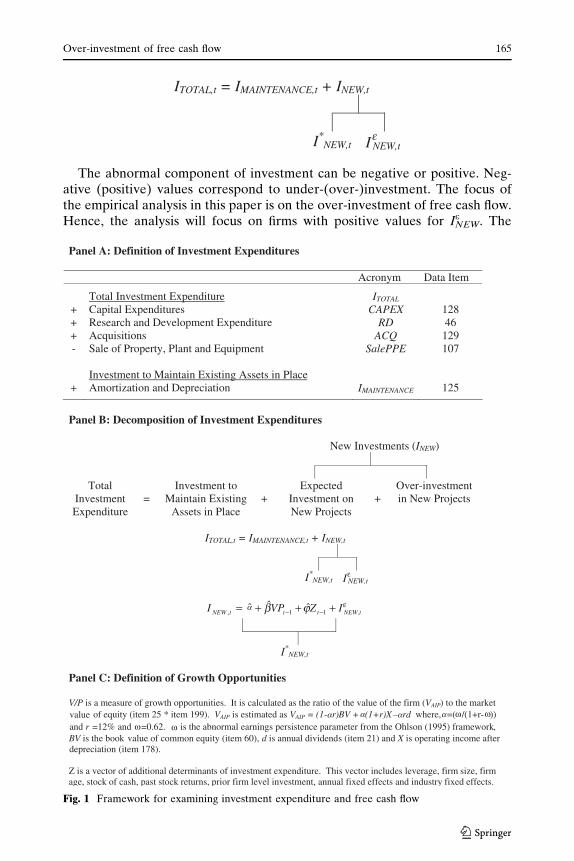
The abnormal component of investment can be negative or positive. Neg-ative (positive) values correspond to under-(over-)investment. The focus ofthe empirical analysis in this paper is on the over-investment of free cash flow.Hence, the analysis will focus on firms with positive values for INEW

e . The

Panel A: Definition of Investment Expenditures

Acronym Data Item

Total Investment Expenditure ITOTAL

+ Capital Expenditures CAPEX 128+ Research and Development Expenditure RD 46+ Acquisitions ACQ 129- Sale of Property, Plant and Equipment SalePPE 107

Investment to Maintain Existing Assets in Place+ Amortization and Depreciation IMAINTENANCE 125

Panel B: Decomposition of Investment Expenditures

New Investments (INEW)

TotalInvestmentExpenditure

=Investment to

Maintain ExistingAssets in Place

+Expected

Investment on New Projects

+Over-investmentin New Projects

ITOTAL,t = IMAINTENANCE,t + INEW,t

I*NEW,t I NEW,t

tNEWtttNEW IZVPI ,11, ˆˆˆ +++= ––

I*NEW,t

Panel C: Definition of Growth Opportunities

V/P is a measure of growth opportunities. It is calculated as the ratio of the value of the firm (VAIP) to the market of equity (item 25 * item 199). VAIP is estimated as VAIP = (1- r) BV + (1+r)X – rd where, =( /(1+r- ))

and =0.62. is the abnormal earnings persistence parameter from the Ohlson (1995) framework,value of common equity (item 60), d is annual dividends (item 21) and X is operating income after

depreciation (item 178).

Z is a vector of additional determinants of investment expenditure. This vector includes leverage, firm size, firmage, stock of cash, past stock returns, prior firm level investment, annual fixed effects and industry fixed effects.

ε

εa

a a a a

b j

ωω ω

ω=12%

valueand rBV is the book

Fig. 1 Framework for examining investment expenditure and free cash flow

ITOTAL,t = IMAINTENANCE,t + INEW,t

I*NEW,t I NEW,t

e


123

Panel D: Reconciliation of the Sources and Uses of Free cash flow

Acronym Data Item TotalsSOURCES:Free cash flow from Existing Assets in Place CFAIP

+ Net Cash flow from Operating Activities CFO 308- Maintenance Investment Expenditure IMAINTENANCE 125+ Research and Development Expenditure RD 46 1

Free cash flow from Growth Opportunities I*NEW

- Expected Investment on New Projects 2

Net Sources of Free cash flow FCF = CFAIP – I*NEW (2) 1-2

USES:Over-Investment I NEW 3

Net Cash Flow to Equity Holders Equity+ Purchase of Common and Preferred Stock 115+ Cash Dividends 127- Sales of Common and Preferred Stock 108 4

Net Cash Flow to Debt Holders Debt+ Long-term Debt Reduction 114- Long-term Debt Issuance 111- Changes in Current Debt 301 5

Change in Financial Assets Fin. Asset + Increase in Cash and Cash Equivalents 274- Change in Short Term Investments 309 6

Other Investments Other Inv. + Increase in Investments 113- Sale of Investments 109 7

Miscellaneous Cash Flows Other- Other Investing Activities 310- Other Financing Activities 312- Exchange Rate Effect 314 8

Net Uses of Free cash flow3+4+5+6+

7+8

D

D

D

e

The following equality will always hold:

FCFt = I NEW,t + Equityt + Debtt + Financial Assett + Other Inv. t + Othert

FCFt

I NEW,t Equityt Debtt FinancialAssett Other Inv.t Othert

e D

D D D

D D

Fig. 1 continued

166 S. Richardson

123

investment expectation model is described in more detail in Section 1.4. Thepredicted value from this expectation model is INEW

* and the residual valuefrom the expectation model is INEW

e . The residual value is my estimate of over-investment.

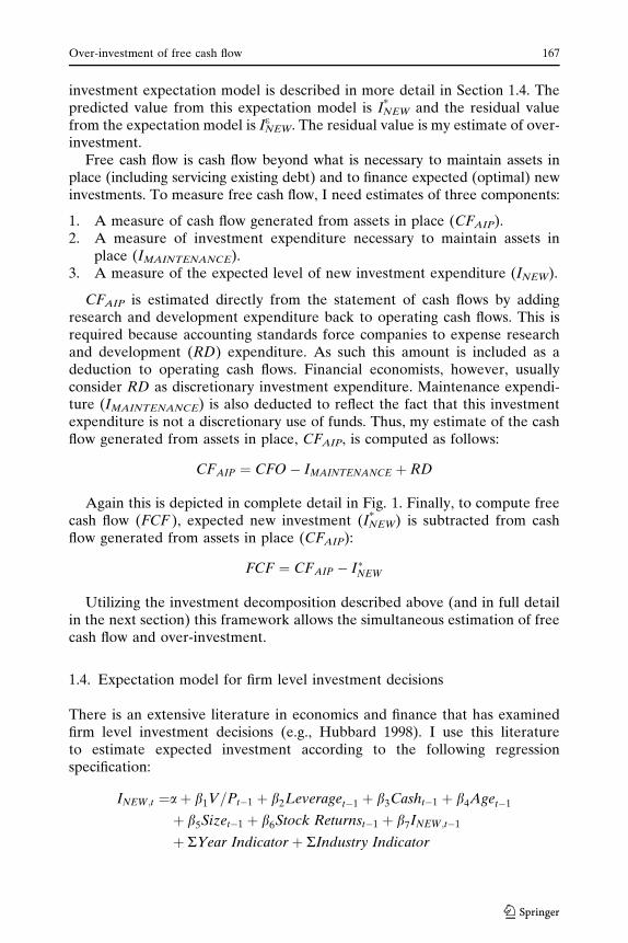
Free cash flow is cash flow beyond what is necessary to maintain assets inplace (including servicing existing debt) and to finance expected (optimal) newinvestments. To measure free cash flow, I need estimates of three components:

1. A measure of cash flow generated from assets in place (CFAIP).2. A measure of investment expenditure necessary to maintain assets in

place (IMAINTENANCE).3. A measure of the expected level of new investment expenditure (INEW).

CFAIP is estimated directly from the statement of cash flows by addingresearch and development expenditure back to operating cash flows. This isrequired because accounting standards force companies to expense researchand development (RD) expenditure. As such this amount is included as adeduction to operating cash flows. Financial economists, however, usuallyconsider RD as discretionary investment expenditure. Maintenance expendi-ture (IMAINTENANCE) is also deducted to reflect the fact that this investmentexpenditure is not a discretionary use of funds. Thus, my estimate of the cashflow generated from assets in place, CFAIP, is computed as follows:

CFAIP ¼ CFO� IMAINTENANCE þ RD

Again this is depicted in complete detail in Fig. 1. Finally, to compute freecash flow (FCF ), expected new investment (INEW

* ) is subtracted from cashflow generated from assets in place (CFAIP):

FCF ¼ CFAIP � I�NEW

Utilizing the investment decomposition described above (and in full detailin the next section) this framework allows the simultaneous estimation of freecash flow and over-investment.

1.4. Expectation model for firm level investment decisions

There is an extensive literature in economics and finance that has examinedfirm level investment decisions (e.g., Hubbard 1998). I use this literatureto estimate expected investment according to the following regressionspecification:

INEW;t ¼aþ b1V=Pt�1 þ b2Leveraget�1 þ b3Casht�1 þ b4Aget�1

þ b5Sizet�1 þ b6Stock Returnst�1 þ b7INEW;t�1

þ RYear Indicator þ RIndustry Indicator


123

The fitted value from the above regression is the estimate of the ex-pected level of new investment, I*

NEW. The unexplained portion (orresidual) is the estimate of over-investment, INEW

e .3 Expected investmentexpenditure on new projects will be an increasing function of growthopportunities. The underlying construct of growth opportunities refers tothe present value of the firm’s options to make future investments (Myers,1977). As researchers we are at a disadvantage when we try to measure thisconstruct, because managers have access to the information pertaining toprospective investment activity and people outside the firm do not. Thestandard approach in the literature has been to use market price relative tosome measure of fundamental value to determine growth opportunities.Tobin’s Q (the ratio of the market value of assets to the current replace-ment cost of those assets) is the most widely used measure of growthopportunities. However, measures such as Q alone do not give a completepicture of the market’s expectations of growth opportunities. Previous re-search that uses book-to-market of equity (BM) and earnings-price ratios(EP) as measures of growth opportunities can be viewed as special cases ofthe residual income valuation model (Penman, 1996). For BM to be asufficient statistic for growth opportunities it must be true that earnings arecompletely transitory. Conversely, for EP to be a sufficient statistic requiresearnings to be completely permanent. However, it is well known thatearnings display a degree of mean reversion in between these two extremes(e.g., Dechow, Hutton, & Sloan, 1999). Thus, using either market-to-bookor price-earnings or some arbitrary combination will generate an inefficientestimate of growth opportunities because knowledge of earnings persistenceis ignored.

Using the residual income framework, it is possible to construct a parsi-monious measure of growth opportunities, incorporating information inmarket price in conjunction with measures of the value of firm’s assets in placeas reflected in book value and current earnings. I start with the premise thatfirm value can be decomposed into two components: value of the assets inplace, VAIP, and the value of growth opportunities, VGO. So firm value, P, canbe represented as:

P ¼ VAIP þ VGO

Firm value, P, is observable. So I need to estimate either VAIP or VGO

directly. A natural starting point is to estimate VAIP using the residual incomeframework. The intuition behind this approach is that the value of assets in

3 I estimate the investment expectation model across all firms which implies that the average over-investment across firm-years is equal to zero. Obviously, this analysis is subject to the standardcriticism of mis-specification in the investment expectation model (with respect to both functionalform and the set of included independent variables). To address these concerns, I consider dif-ferent sets of independent variables in the investment model (see Section 3) and perform analysisusing raw and ranked data as well as a portfolio approach that assumes measurement error isuncorrelated across portfolios (discussed in Section 3.2). My results are robust to all of thesespecifications.

168 S. Richardson

123

place will manifest itself in current book values and earnings. On the otherhand growth opportunities are yet to be accounted for and will represent thedifference between observed firm value and an estimate of the value of assetsin place.

Assuming price is equal to discounted expected dividends, accountinginformation articulates via the clean-surplus relation, and abnormal earningsfollow an auto-regressive process with persistence parameter, x, it is possibleto express the value of assets in place, VAIP as:

VAIP ¼ ð1� arÞBV þ að1þ rÞX � ard

where BV is the book value of common equity, X is earnings, r is the discountrate, d is dividends, x is a fixed persistence parameter restricted to be positiveand less than one, and a =(x/(1+r–x).4 VAIP reflects the value of the firmindicated by current book values and current earnings. Thus, it provides anestimate of firm value attributable to assets in place. It is useful to note thatthis specification of firm value introduced by Ohlson (1995) is an estimate offirm value absent growth opportunities. Additional research by Feltham andOhlson (1996) allows for the presence of new positive NPV projects. Undertheir model, firm value is similar to the algebraic expression above except foran additional term that captures growth opportunities. This frameworksimultaneously captures market value relative to both book value and earn-ings in an accepted valuation framework. It is easily implemented, as the onlyrequired inputs are price, book value, earnings, dividends, a discount rate andan earnings persistence parameter.5 Thus, to capture growth opportunitiesfrom accounting and market information, V/P is measured as the ratio of VAIP

to market value instead of the standard Tobin’s Q measure.6

It is useful to discuss how V/P relates to both book-to-market and earnings-to-price ratios. V/P is a linear combination of BM and EP (the numerator ofV/P is a weighted average of book values and earnings). BM can be expressedas the summation of future abnormal return on equity (see e.g., Fairfield,

4 In the empirical implementation of this model I use a measure of operating earnings. This isdriven by practical considerations relating to the predictability of future abnormal earnings.Measures of bottom line earnings do not perform as well as measures of operating earnings inpredicting abnormal earnings. This is largely due to the lower persistence of the transitory itemsthat are included in measures of comprehensive or bottom line income (e.g., Dechow et al., 1999).5 Specifically, the framework is flexible enough to allow inter-temporal and cross-sectional vari-ation of these last two parameters. However, for my purposes I assume a constant discount rate of12 percent and the persistence parameter of 0.62 as reported in Dechow et al. (1999). I have re-performed all analyses using (i) industry specific earnings persistence parameters, and (ii) firmspecific cost of capital estimates from the CAPM model. The key inference that over-investment isconcentrated in firms with positive free cash flow is unaffected by these alternative estimationapproaches.6 The reciprocal is preferred for two reasons. First, the distribution of the reciprocal is less skewedleading to more desirable properties for statistical tests. Second, the measure is continuousthrough zero such that firms with negative book values are ranked similar to high growth firms.Note that using the reciprocal (i.e., V/P) means that the expected relation between investment andgrowth opportunities is negative.


123

1994; Wilcox, 1984). The key driver of BM is the expected level of abnormalfuture return on equity for the remainder of the firm’s operating horizon andgrowth in book values. However, it is important to realize that BM can be lowdue to high current performance (see e.g., Fairfield, 1994; Penman, 1991,1996). Firms such as Coca-Cola and Kroger are good examples. These firmshave very low BM (in bottom decile) yet they have moderate levels of V/P(around the median). Hence, using BM alone will mis-classify these firms ashaving high growth opportunities.

Similarly, using EP alone will lead to mis-classification. The key driver ofEP is the growth in future abnormal earnings. However, EP ratios alone aredifficult to interpret in the presence of temporarily depressed current earnings.To discriminate between firms that have low EP due to transitory earnings, asopposed to growth opportunities, it is necessary to look at the information inBM. Firms with low levels of EP BM are the firms with the greatest growthopportunities.

I include additional control variables that have been shown in prior re-search to be determinants of investment decisions, including leverage, firmsize, firm age, the level of cash, past stock returns and prior firm levelinvestment (e.g., Barro 1990; Bates, 2005; Hubbard, 1998; Lamont, 2000).Previous research has documented a sensitivity of firm level investment tothese measures. Firm level investment is lessened when it is more difficult toraise additional cash to finance the new investment as captured by leverage,firm size, firm maturity and level of cash (e.g., Fazzari et al., 1988; Hubbard,1998). Prior stock returns is included as an additional variable to capturegrowth opportunities not reflected in V/P (Barro, 1990; Lamont, 2000) andprior firm level investment is included to capture non-modeled firm charac-teristics that impact investing decisions. I also include indicator variables forindustry membership and temporal effects to capture additional variation ininvestment expenditure that are not explained by my measures of growthopportunities and financing constraints. It is important to note that includingthese additional variables may reduce the power of my tests to capture over-investment. For example, if over-investment is concentrated in industrygroups, in particular time periods or is concentrated in certain firms then themodel may inappropriately classify abnormal investment as normal invest-ment, effectively controlling for the effect that I am trying to document. Toaddress this possibility, multiple investment expectation models are examinedin Section 3.

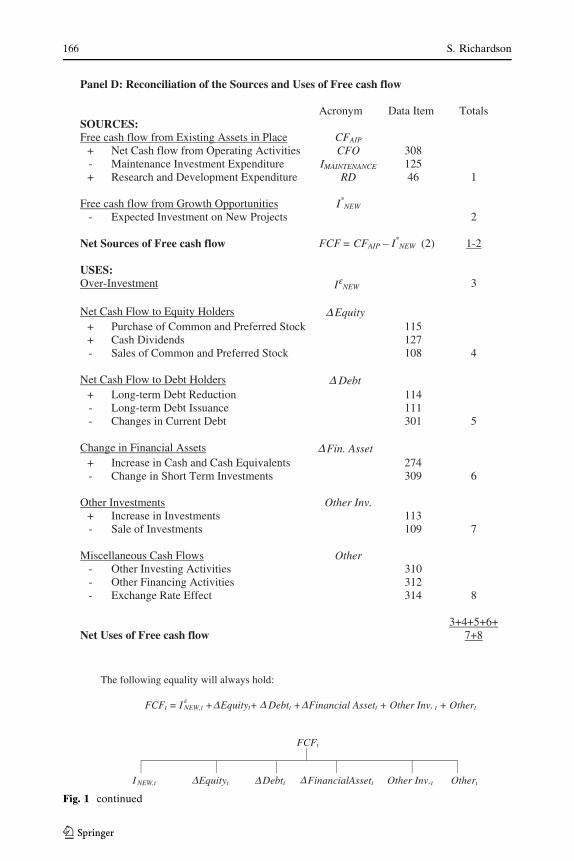
1.5. Uses of free cash flow

The focus of this paper is the over-investment of free cash flow. However,over-investment is but one of many alternate uses of free cash flow. Panel D ofFig. 1 depicts the sources and uses of free cash flow. This analysis character-izes all possible uses of the free cash flow derived in Section 1.3. Usinginformation obtained from the statement of cash flows, I am able to allocatefree cash flow flows into six categories. This is simply a re-characterization of

170 S. Richardson

123

the statement of cash flows, where cash generated must equal cash used. Thesix categories are: (i) over-investment, INEW

e , (ii) net payments to sharehold-ers, DEquity, (iii) net principal payments to debt-holders, DDebt, (iv) netchange in financial assets, DFinancial Asset, (v) Other Investments and (vi)miscellaneous cash flows, Other. This is represented by the following identity:

FCFt �IeNEW;t þ DEquityt þ DDebtt þ DFinancial Assett

þOther Investmentst þOthert

The final two categories contain miscellaneous reconciling items that arenot important empirically (very little variation in the sample). The mainconcern from the perspective of shareholders is the first category, over-investment, because this imposes substantial agency costs on shareholders.However, it is less clear what the best use of free cash flow is beyond avoidingover-investment. Payments to shareholders will be affected by the tax status ofthe firm’s investor base (Allen & Michaely, 2003). In addition, payments toboth shareholders and debt-holders will impact the capital structure of thefirm. To the extent that management is seeking an optimal capital structure, itis difficult to determine what the optimal distribution of free cash flow shouldbe. Retention of free cash flow in the form of financial assets is also an optionavailable to management. The optimal level of free cash flow to be retainedwill be a function of firm specific characteristics such as variability of cash flowand ability to access external capital markets (e.g., Harford, 1999). Firms withmore volatile cash flows will want to retain cash for future periods when cashflow is low, and firms who find it more difficult to raise external capital willdesire larger cash holdings (e.g., Opler et al., 1999). My primary focus is onthe extent of over-investment and the role that governance structures can playin mitigating over-investment. I leave detailed examination of how firms usefree cash flow (other than over-investing) to future research.

2. Data and sample selection

The main empirical tests employ financial statement data from the Compustatannual database (inclusive of active and inactive securities). I exclude financialinstitutions from my analysis (SIC codes between 6000 and 6999) because thedemarcation between operating, investing, and financing activities is ambig-uous for these firms. The sample period covers the fiscal years 1988–2002 with58,053 firm-year observations.

In the empirical analysis that follows I scale all financial variables byaverage total assets (results are similar using sales as an alternative deflator).To minimize the influence of outliers I delete firms where the deflated value offree cash flow or any of the potential uses of free cash flow exceeds one inabsolute value. The measure of growth opportunities, V/P, is winsorized by re-coding observations less (greater) than the 1st (99th) percentile to the 1st(99th) percentile. In unreported tests, I re-perform all analyses using rank


123

regressions according to the procedure outlined in Iman and Conover (1979).Results from this analysis are similar to those reported in the text.

3. Results

3.1. Analysis of investment expenditure and free cash flow

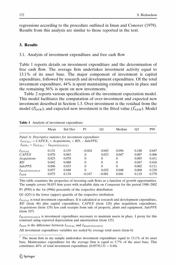
Table 1 reports details on investment expenditure and the determination offree cash flow. The average firm undertakes investment activity equal to13.1% of its asset base. The major component of investment is capitalexpenditure, followed by research and development expenditure. Of the totalinvestment expenditure, 44% is spent maintaining existing assets in place andthe remaining 56% is spent on new investments.7

Table 2 reports various specifications of the investment expectation model.This model facilitates the computation of over-investment and expected newinvestment described in Section 1.3. Over-investment is the residual from themodel (INEW

e ), and expected new investment is the fitted value (INEW* ). Model

Table 1 Analysis of investment expenditure

Mean Std Dev P1 Q1 Median Q3 P99

Panel A: Descriptive statistics for investment expenditureITOTAL;t ¼ CAPEXt þAcquisitionst þ RDt � SalePPEt

INEW;t ¼ ITOTAL;t � IMAINTENANCE;t

ITOTAL 0.131 0.135 –0.024 0.043 0.094 0.180 0.647CAPEX 0.070 0.083 0 0.023 0.047 0.087 0.406Acquistions 0.025 0.078 0 0 0 0.005 0.411RD 0.042 0.088 0 0 0 0.047 0.416SalePPE 0.006 0.033 0 0 0 0.002 0.111IMAINTENANCE 0.057 0.048 0 0.032 0.048 0.068 0.230INEW 0.075 0.134 –0.167 –0.001 0.041 0.119 0.578

This table examines the properties of investing cash flows as a function of growth opportunities.The sample covers 58,053 firm years with available data on Compustat for the period 1988–2002

P1 (P99) is the 1st (99th) percentile of the respective distribution

Q1 (Q3) is the lower (upper) quartile of the respective istribution

ITOTAL is total investment expenditure. It is calculated as research and development expenditure,RD (item 46) plus capital expenditure, CAPEX (item 128) plus acquisition expenditure,Acquisitions (item 129) less cash receipts from sale of property, plant and equipment, SalePPE(item 107)

IMAINTENANCE is investment expenditure necessary to maintain assets in place. I proxy for thisconstruct using reported depreciation and amortization (item 125)

INEW is the difference between ITOTAL and IMAINTENANCE

All investment expenditure variables are scaled by average total assets (item 6)

7 The mean firm in my sample undertakes investment expenditure equal to 13.1% of its assetbase. Maintenance expenditure for the average firm is equal to 5.7% of the asset base. Thisconstitutes 44% of total investment expenditure (0.057/0.131 = 0.44).

172 S. Richardson

123

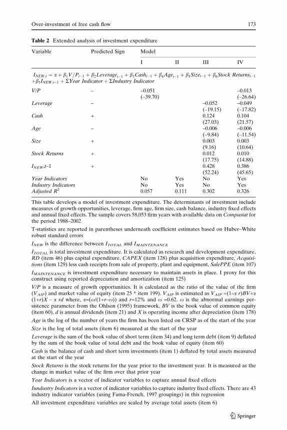
Table 2 Extended analysis of investment expenditure

Variable Predicted Sign Model

I II III IV

INEW;t ¼ aþ b1V=Pt�1 þ b2Leveraget�1 þ b3Casht�1 þ b4Aget�1 þ b5Sizet�1 þ b6Stock Returnst�1

þb7INEW;t�1 þ RYear Indicator þ RIndustry Indicator

V/P – –0.051(–39.70)

–0.013(–26.64)

Leverage – –0.052(–19.15)

–0.049(–17.82)

Cash + 0.124(27.03)

0.104(21.57)

Age – –0.006(–9.84)

–0.006(–11.54)

Size + 0.003(9.16)

0.003(10.64)

Stock Returns + 0.012(17.75)

0.010(14.88)

INEW,t–1 + 0.428(52.24)

0.386(45.65)

Year Indicators No Yes No YesIndustry Indicators No Yes No YesAdjusted R2 0.057 0.111 0.302 0.326

This table develops a model of investment expenditure. The determinants of investment includemeasures of growth opportunities, leverage, firm age, firm size, cash balance, industry fixed effectsand annual fixed effects. The sample covers 58,053 firm years with available data on Compustat forthe period 1988–2002

T-statistics are reported in parentheses underneath coefficient estimates based on Huber–Whiterobust standard errors

INEW is the difference between ITOTAL and IMAINTENANCE

ITOTAL is total investment expenditure. It is calculated as research and development expenditure,RD (item 46) plus capital expenditure, CAPEX (item 128) plus acquisition expenditure, Acquisi-tions (item 129) less cash receipts from sale of property, plant and equipment, SalePPE (item 107)

IMAINTENANCE is investment expenditure necessary to maintain assets in place. I proxy for thisconstruct using reported depreciation and amortization (item 125)

V/P is a measure of growth opportunities. It is calculated as the ratio of the value of the firm(VAIP) and market value of equity (item 25 * item 199). VAIP is estimated as VAIP =(1–a r)BV+a(1+r)X – a rd where, a=(x/(1+r–x)) and r=12% and x =0.62. x is the abnormal earnings per-sistence parameter from the Ohlson (1995) framework, BV is the book value of common equity(item 60), d is annual dividends (item 21) and X is operating income after depreciation (item 178)

Age is the log of the number of years the firm has been listed on CRSP as of the start of the year

Size is the log of total assets (item 6) measured at the start of the year

Leverage is the sum of the book value of short term (item 34) and long term debt (item 9) deflatedby the sum of the book value of total debt and the book value of equity (item 60)

Cash is the balance of cash and short term investments (item 1) deflated by total assets measuredat the start of the year

Stock Returns is the stock returns for the year prior to the investment year. It is measured as thechange in market value of the firm over that prior year

Year Indicators is a vector of indicator variables to capture annual fixed effects

Iundustry Indicators is a vector of indicator variables to capture industry fixed effects. There are 43industry indicator variables (using Fama-French, 1997 groupings) in this regression

All investment expenditure variables are scaled by average total assets (item 6)


123

I comprises only the accounting based measure of growth opportunities, V/P.The regression estimates reported in this table are for the pooled sample withHuber–White robust standard errors, which are a generalization of theWhite (1980) standard errors that are robust to both serial correlation andheteroskedasticity (Rogers, 1993). The coefficient estimate for b1 is –0.051. Togive some economic interpretation to the strength of this relation, an inter-quartile change in V/P of 0.582 [the first (third) quartile of the V/P distributionis 0.310 (0.892)], corresponds to an additional 0.030 (0.582 * 0.051) in newinvestment expenditure. Alternatively stated, an inter-quartile change ingrowth opportunities translates to additional investment equal to three per-cent of the asset base of the firm. While this number appears small it isimportant to remember that V/P captures the expected benefit from currentand expected investment expenditure in all future periods. The point estimatefrom this regression specification captures only investment in the currentperiod. In unreported analyses this specification was estimated by industry andindustry-year groupings (using Fama & French, 1997 industry definitions andthe Fama & Macbeth, 1973 technique of estimating regression coefficients bygroup and averaging results across groups). The results are very similar tothose reported in the table. Across all regression specifications the coefficienton V/P is significantly negative.

The model of investment expenditure in the first column of Table 2includes only growth opportunities as an explanatory variable. The remainingmodels expand the set of included determinants (each specification reportsresults with Huber–White robust standard errors). The second model showsthat including only industry and annual fixed effects explains 11.1% of thevariation in INEW. The control variables leverage, cash balance, firm age, firmsize, prior stock returns and prior firm level investment expenditure explain30.2% of the variation (model III). Including all of the variables increasesthe explanatory power to 32.6% (model IV). All control variables load asexpected—new investment expenditure is increasing in firm size, prior cashholdings, prior stock returns and prior investment activity and decreasingin firm age and leverage. In subsequent analyses decomposing INEW intoexpected investment (INEW

* ) and over-investment (INEWe ) I use model IV.

Later results examining the relation between over-investment and free cashflow are similar if I instead use any of the models in Table 2.

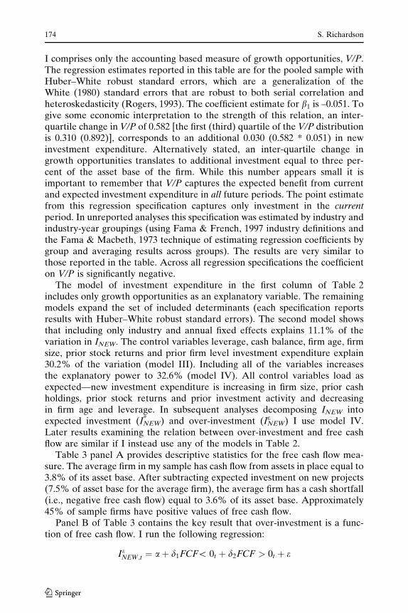
Table 3 panel A provides descriptive statistics for the free cash flow mea-sure. The average firm in my sample has cash flow from assets in place equal to3.8% of its asset base. After subtracting expected investment on new projects(7.5% of asset base for the average firm), the average firm has a cash shortfall(i.e., negative free cash flow) equal to 3.6% of its asset base. Approximately45% of sample firms have positive values of free cash flow.

Panel B of Table 3 contains the key result that over-investment is a func-tion of free cash flow. I run the following regression:

IeNEW;t ¼ aþ d1FCF\ 0t þ d2FCF > 0t þ e

174 S. Richardson

123

Ta

ble

3A

na

lysi

so

ffr

ee

cash

flo

wa

nd

ov

er-i

nv

est

men

t

Me

an

Std

De

vP

1Q

1M

ed

ian

Q3

P9

9

Pa

nel

A:

Des

crip

tiv

est

ati

stic

sfo

rfr

eeca

shfl

ow

FC

Ft¼

CF

AIP;t�

I� NE

W;t

I NE

W*

isth

efi

tted

va

lue

fro

m:

I NE

W;t¼

aþ

b1V=P

t�1þ

b2L

ever

age t�

1þ

b 3C

ash

t�1þ

b 4A

ge t�

1þ

b 5S

ize t�

1þ

b 6S

tock

Ret

urn

s t�

1þ

b 7I N

EW;t�

1þ

RY

ear

Ind

ica

torþ

RIn

du

stry

Ind

icato

r

CF

AIP

0.0

380

.14

5–

0.4

45

–0

.01

90

.042

0.1

060

.41

4I N

EW

*0

.075

0.0

76

–0

.05

80

.02

40

.059

0.1

120

.32

5I N

EW

e0

0.1

10

–0

.24

9–

0.0

50

–0

.01

20

.030

0.4

14

FC

F–

0.0

36

0.1

53

–0

.57

3–

0.0

92

–0

.01

20

.045

0.2

88

Pan

elB

:R

elati

on

bet

wee

no

ver

-in

ves

tmen

t(I

NE

We

)an

dfr

eeca

shfl

ow

(FC

F)

Ie NE

W;t¼

aþ

d 1F

CF\

0tþ

d 2F

CF[

0tþ

e

Mo

de

la

d 1d 2

Ad

just

edR

2

Po

ole

d0

.002

(2.6

5)0

.111

(15

.19

)0

.171

(13

.78

)0

.03

2

F-s

tati

stic

for

test

d 1=d 2

:4

0.8

7*

**

Fa

ma

-Ma

cBe

th(1

5y

ea

rs)

0.0

02(1

.54)

0.1

15(9

.47)

0.1

72(1

2.1

3)

0.0

37

T-s

tati

stic

fro

ma

nn

ua

lco

effi

cie

nt

est

ima

tes

for

test

:d 1

=d 2

:2

.35

**

*

Th

eta

ble

ex

am

ine

sth

ep

rop

ert

ies

of

fre

eca

shfl

ow

an

dh

ow

itre

late

sto

ov

er-i

nv

est

me

nt.

All

va

ria

ble

sa

resc

ale

db

ya

ve

rag

eto

tal

ass

ets

.T

he

sam

ple

cov

ers

58

,05

3fi

rmy

ea

rsw

ith

av

ail

able

da

tao

nC

om

pu

sta

tfo

rth

ep

eri

od

19

88–

20

02

T-s

tati

stic

sa

rere

po

rte

din

pa

ren

the

ses

un

de

rnea

thco

effi

cie

nt

est

ima

tes.

**

*in

dic

ate

ssi

gn

ifica

nt

dif

fere

nce

at

the

1%

lev

el

Fo

rth

ep

oo

led

reg

ress

ion

sI

rep

ort

t-v

alu

es

ba

sed

on

Hu

be

r–W

hit

ero

bu

stst

an

da

rde

rro

rs

Fo

rth

ein

du

stry

an

din

du

stry

-ye

ar

gro

up

reg

ress

ion

sth

ep

ara

me

ter

est

ima

tes

an

da

reth

ew

eig

hte

da

ve

rag

e(u

sin

gth

esq

ua

rero

ot

of

the

nu

mb

er

of

ob

serv

ati

on

sin

ea

chg

rou

pa

sth

ew

eig

ht)

of

ind

ivid

ua

lg

rou

pre

gre

ssio

np

ara

me

ters

.T

est

sta

tist

ics

are

ba

sed

on

the

acr

oss

gro

up

va

ria

tio

nin

the

sep

ara

me

ters

P1

(P9

9)is

the

1st

(99

th)

pe

rce

nti

leo

fth

ere

spe

ctiv

ed

istr

ibu

tio

n

Q1

(Q3

)is

the

low

er

(up

pe

r)q

ua

rtil

eo

fth

ere

spe

ctiv

ed

istr

ibu

tio

n


123

Table

3co

nti

nu

ed

I NE

Wis

the

dif

fere

nce

be

twee

nI T

OT

AL

an

dI M

AIN

TE

NA

NC

E

I TO

TA

Lis

tota

lin

ve

stm

ent

ex

pe

nd

itu

re.

Itis

calc

ula

ted

as

rese

arch

an

dd

ev

elo

pm

en

te

xp

en

dit

ure

,R

D(i

tem

46

)p

lus

cap

ita

le

xp

en

dit

ure

,C

AP

EX

(ite

m1

28

)p

lus

acq

uis

itio

ne

xp

en

dit

ure

,A

cqu

isit

ion

s(i

tem

12

9)

less

cash

rece

ipts

fro

msa

leo

fp

rop

ert

y,

pla

nt

an

de

qu

ipm

ent,

Sa

leP

PE

(ite

m1

07

)

I MA

INT

EN

AN

CE

isin

ve

stm

en

te

xp

en

dit

ure

ne

cess

ary

tom

ain

tain

ass

ets

inp

lace

.I

pro

xy

for

this

con

stru

ctu

sin

gre

po

rted

de

pre

cia

tio

na

nd

am

ort

iza

tio

n(i

tem

12

5)

I NE

W*

isth

efi

tte

dv

alu

efr

om

reg

ress

ion

mo

de

lIV

inT

able

2.

Itis

an

est

ima

teo

fth

ee

xp

ect

ed

leve

lo

fin

ve

stm

ent

I NE

We

isth

ere

sid

ua

lfr

om

reg

ress

ion

mo

de

lIV

inT

able

2.

Itis

an

est

ima

teo

fo

ver

-in

ve

stm

ent

CF

AIP

isca

shfl

ow

fro

mo

pe

rati

ng

act

ivit

ies

aft

er

ma

inte

na

nce

inv

est

men

te

xp

en

dit

ure

.It

isca

lcu

late

da

sca

shfr

om

op

era

tio

ns

(ite

m3

08

)le

ssI M

AIN

TE

NA

NC

E

plu

sre

sear

cha

nd

de

velo

pm

en

te

xp

en

dit

ure

(ite

m4

6)

FC

Fis

CF

AIP

less

I NE

W*

.F

CF

isca

shfl

ow

be

yo

nd

tha

tn

ece

ssa

ryto

ma

inta

ina

sse

tsin

pla

ce(i

ncl

ud

ing

serv

icin

ge

xis

tin

gd

eb

to

bli

ga

tio

ns)

an

dfi

na

nce

ex

pe

cte

dn

ew

inv

est

men

ts(i

.e.,

fre

eca

shfl

ow

)

FC

F<

0(F

CF

>0

)is

eq

ua

lto

FC

Ffo

rv

alu

eso

fF

CF

less

(gre

ate

rth

an

)ze

roa

nd

zero

oth

erw

ise

All

inv

est

men

ta

nd

cash

flo

wv

ari

ab

les

are

sca

led

by

av

era

ge

tota

la

sse

ts(i

tem

6)

176 S. Richardson

123

FCF < 0 (FCF > 0) is equal to FCF for values of FCF less (greater than)zero and zero otherwise. This allows the relation between over-investment andfree cash flow to be asymmetric. In particular, allowing the slope coefficient tovary based on the sign of free cash flow reveals that over-investment is con-centrated in firms with positive free cash flow (the estimate of d1 is 0.111 andthe estimate of d2 is 0.171, significantly different at the 1% level). Panel Breports both pooled regression estimates (using robust standard errors) as wellas average estimates from annual regressions. Out of the fifteen annualregressions, the estimate for d2 is statistically greater than the estimate for d1 ineleven years. When firms have do not have free cash flow, (i.e., FCF < 0) thepossibility of over-investment is mitigated as the firm is forced to accessexternal markets to raise funds necessary for any additional investment.Capital markets serve an additional monitoring role in disciplining managerialuse of funds. The regression results in Table 3 support H1 by showing that firmswith positive free cash flow are more likely to over-invest on average and thenfor each additional dollar of free cash flow they over-invest more. It isimportant to note the relatively low explanatory power from this regressionspecification. The model describing free cash flow as the determinant of over-investment only explains 3.2% of the variation. However, this explanatorypower is incremental to the set of other determinants of firm level investmentexpenditure (which was 32.6% for model IV). So, the combined framework isable to explain a significant portion of the cross-sectional variation in invest-ment expenditure and find a statistically significant relation between over-investment and free cash flow.

While not the focus of my paper, the regression results in Table 3 alsorelate to under-investment. The positive coefficient on d1 indicates that firmswith negative free cash flow experience less over-investment (or equivalentlystated more under-investment as the mean value of over-investment for thissub-sample of firms is negative). This relation is consistent with the notion thatfirms subject to cash short falls from operating activities scale back oninvestment activity. But it is important to note that the strength of the relationbetween abnormal investment and free cash flow is muted for firms withnegative free cash flow (i.e., d1 is much smaller than d2) because these firmsare able to raise additional cash from external financial markets.

Panel A of Table 4 reports the distributional properties of the free cashflow measure and the various uses of free cash flow. There is little variation inthe ‘‘other investments’’ and miscellaneous ‘‘other’’ category—I ignore theseuses in subsequent discussion. The breakdown of each additional dollar of freecash flow is shown in panel B of Table 4. I examine firm-year observationswith positive free cash flow separately from negative free cash flow observa-tions. For each sample, I average the different uses of free cash flow andexpress each use as a percentage of available free cash flow. This partition onthe sample emphasizes how the use of free cash flow varies based on the signof free cash flow.

For firms with positive free cash flow (44.6% of the sample) the average useof a dollar of free cash flow is as follows: 20% is over-invested, 13% is paid out


123

Table 4 Analysis of alternative uses of free cash flow. The sample covers 58,053 firm years withavailable data on Compustat for the period 1988–2002

Mean Std Dev P1 Q1 Median Q3 P99

Panel A: Descriptive statistics for how free cash flow is usedFCF –0.036 0.153 –0.573 –0.092 –0.012 0.045 0.288INEWe 0 0.110 –0.249 –0.050 –0.012 0.030 0.414

DEquity –0.021 0.132 –0.665 –0.008 0 0.017 0.196DDebt –0.017 0.115 –0.461 –0.041 0 0.025 0.251D FinancialAsset 0.001 0.127 –0.409 –0.025 0.000 0.027 0.441Other Inv. 0.002 0.058 –0.160 0 0 0 0.182Other –0.002 0.075 –0.293 –0.003 0 0.008 0.189

Panel B: How free cash flow is used

Sources and Uses FCF > 0 Firm-years(n = 25,897)

FCF < 0 Firm-years(n = 32,156)

Average Percent (%) Average Percent (%)

SourcesFCF 0.075 100 –0.126 100UsesINEWe 0.015 20 –0.012 10

DEquity 0.009 13 –0.046 37DDebt 0.011 15 –0.039 31DFinancialAsset 0.031 41 –0.022 18Other Inv. 0.004 6 0.000 0Other 0.004 5 –0.006 5

P1 (P99) is the 1st (99th) percentile of the respective distribution

Q1 (Q3) is the lower (upper) quartile of the respective distribution

DEquity is the net cash returned to shareholders for the period. It is calculated as the sum ofrepurchases, (item 115) and dividends (item 127) less cash raised from stock issuance (item 108)

DDebt is the net cash returned to debtholders for the period. It is calculated as long term debtreduction (item 114) less long term debt issuance (item 111) less changes in current debt (item 301)

DFinancial Assets is the change in cash holdings. It is calculated as change in cash (item274) lesschange in short term investments (item 309)

Other Investments is other investments made. It is calculated as increase in investments (item113)less sale of investments (item 109)

Other includes all other categories on the statement of cash flows not included in DEquity, DDebt,DFinancial Assets, INEW

e and Other Investments. It is calculated as the negative of the sum of exchangerate effects (item 314), other investing activities (item 310) and other financing activities (item 312)

FCF is CFAIP less INEW* . FCFs cash flow beyond that necessary to maintain assets in place

(including servicing existing debt obligations) and finance expected new investments

CFAIP is cash flow from operating activities after maintenance investment expenditure. It is cal-culated as cash from operations (item 308) less IMAINTENANCE plus research and developmentexpenditure (item 46)

INEW is the difference between ITOTAL and IMAINTENANCE. INEW represents investment expen-diture after maintenance of existing assets in place. ITOTAL is total investment expenditure. It iscalculated as research and development expenditure, RD (item 46) plus capital expenditure,CAPEX (item 128) plus acquisition expenditure, Acquisitions (item 129) less cash receipts fromsale of property, plant and equipment, SalePPE (item 107). IMAINTENANCE is investment expen-diture necessary to maintain assets in place. I proxy for this construct using reported depreciationand amortization (item 125)

178 S. Richardson

123

to shareholders, 15% is paid out to debt-holders, 41% is retained in financialassets, and the remaining 11% is spread across the other categories. For firmswith negative free cash flow, the breakdown is quite different. The free cashflow shortfall is financed as follows: 10% is under-invested, 37% is receivedfrom shareholders, 31% is received from to debt-holders, 18% is financedfrom existing financial assets, and the remaining 5% is spread across the othercategories. It is clear that firms with cash shortfalls raise additional fundsthrough equity and debt offerings and also by running down existing cashbalances. For firms with positive free cash flow, the two main uses areretention in the form of financial assets and over-investment. Consistent withthe regression results in Table 3 and the agency cost explanation, the positiverelation between over-investment and free cash flow is concentrated in thoseobservations where free cash flow is positive.

3.2. Robustness tests and limitations for the primary hypothesis

To address concerns about the robustness of the primary finding of a positiverelation between over-investment and free cash flow I perform several addi-tional tests (all unreported). The finding that over-investment is concentratedin firms with positive free cash flow is supported by all of these additional tests.

3.2.1. Alternative measures of growth opportunities

I examine the strength of the relation between over-investment and free cashflow for alternative measures of growth opportunities. Alternate measures forgrowth opportunities include book-to-market of equity, earnings-to-price ra-tios and Tobin’s Q. I examine these variables (along with a factor scorecombination of the variables) instead of V/P and continue to find a strongpositive relation between over-investment and free cash flow with thesealternate price-based measures of growth opportunities.

There is also the possibility that market price has already incorporatedthe likelihood of over-investment and the strength of governance mecha-nisms. This will impact the use of price-based measures to identify over-investment. The bias that this introduces into my empirical analysis is notimmediately clear. However, I have replicated my analysis of over-invest-ment and free cash flow using only a price-free estimate of growthopportunities (using the industry median level of investment as a bench-mark). I compare INEW for each firm to the industry median level of INEW,denoted as INEW

IND . My measure of over-investment (INEWe ) is then the

Table 4 continued

INEW* is the fitted value from regression model IV in Table 2. It is an estimate of the expected level

of investment

INEWe is the residual from regression model IV in table 2. It is an estimate of over-investment

All cash flow and investment variables are scaled by average total assets


123

difference between INEW and INEWIND and my estimate of expected investment

(INEW* ) is equal to INEW

IND . Using this price-free estimation I still findover-investment concentrated in firms with positive values of free cash flow.Re-estimating the regression equation in panel B of Table 3, I find that d2

is statistically greater than d1 in fourteen out of the 15 years (i.e., therelation between over-investment and free cash flow continues to be con-centrated in firms with positive free cash flow consistent with the agencycost explanation).

The algebraic representation of VAIP presented in Section 1.4 is equal to thevalue of the firm with unbiased accounting and no positive NPV projects. Inpractice, accounting is systematically biased and firms face positive NPVproject choices. Thus, my estimate of growth opportunities will capture notonly the positive NPV projects but also the impact of conservative accountingpractices. This could be a problem as I include research and developmentexpenditure (RD) as part of investments. To mitigate the problem of con-servative accounting on my empirical analysis, I have performed all analysesexcluding firm year observations where the market-to-book ratio exceeds 5 orRD exceeds 25% of sales. These exclusions do not impact the key inferencethat over-investment is concentrated in firms with positive free cash flow.

3.2.2. Measurement error in over-investment and free cash flow

The reduced form investment model that I examine can also be criticized formeasurement error. To mitigate this concern, I utilize a portfolio approach tore-estimate the relation between over-investment and free cash flow. I ran-domly sort firms into 200 portfolios and then calculate the mean value forover-investment and free cash for each portfolio. Next, I perform a regressionof mean over-investment on mean free cash flow for these 200 portfolios. Theresulting regression has an adjusted R2 of 0.045 and a coefficient of 0.195 onfree cash flow. Similar results are obtained using median values. To the extentthat measurement error is uncorrelated across these ‘‘averaged’’ randomportfolios the positive relation between over-investment and free cash flow isnot attributable to measurement error.8

In unreported tests I also include a measure of the volatility of past cash flowsas an additional control variable. I do not include the cash flow volatility variablein the main tests as it greatly reduces the sample size (to 34,112 firm-yearobservations) because I require a sufficient time series for each firm to be able toestimate operating cash flow volatility. As expected, this variable is negatively

8 It is not critical for my analysis that my investment model is free from error. I only need to beable to identify a measure of unexpected (under/over) investment that is correlated with trueunexpected (under/over) investment. This is likely to be achieved given that my model of expectedinvestment expenditure is drawn from prior research. The theoretical foundation for the reducedform model, the robustness of the relation (between over-investment and free cash flow) toalternative specifications, the concentration of the relation in firms with positive free cash flow andcross-sectional variation in the relation based on the strength of governance structures (see Sec-tion 4) allspeaks to an economic result and not merely a spurious correlation.

180 S. Richardson

123

related to investment expenditure. More importantly, including this variabledoes not affect the positive relation between over-investment and free cash flow.

3.2.3. Is the relation between free cash flow and over-investment mechanical?

There is a concern of a potential mechanical relation between free cash flowand over-investment as estimated from this framework. This concern arisesbecause the measure of free cash flow can be re-written as (CFAIP– INEW+INEWe ). Thus, any association with over-investment might be mechanical.

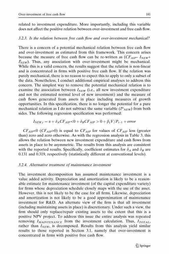
While this is a valid concern, the results suggest that the relation is non-linearand is concentrated in firms with positive free cash flow. If the relation waspurely mechanical, there is no reason to expect this to apply to only a subset ofthe data. Nonetheless, I conduct additional empirical analyses to address thisconcern. The simplest way to remove the potential mechanical relation is toexamine the association between INEW (i.e., all new investment expenditureand not the estimated normal level of new investment) and the measure ofcash flows generated from assets in place including measures of growthopportunities. In this specification, there is no longer the potential for a puremechanical relation as I do not subtract the same variable (I*NEW) from bothsides. The following regression specification was performed:

INEW;t ¼ aþ dACFAIP\0þ dBCFAIP > 0þ b1V=Pt�1 þ error

CFAIP<0 (CFAIP>0) is equal to CFAIP for values of CFAIP less (greaterthan) zero and zero otherwise. As with the regression analysis in Table 3, thisallows the relation between new investment expenditure and cash flows fromassets in place to be asymmetric. The results from this analysis are consistentwith the reported results. Specifically, coefficient estimates for dA and dB are0.131 and 0.319, respectively (statistically different at conventional levels).

3.2.4. Alternative treatment of maintenance investment

The investment decomposition has assumed maintenance investment is avalue added activity. Depreciation and amortization is likely to be a reason-able estimate for maintenance investment (of the capital expenditure variety)for firms whose depreciation schedule closely maps with the use of the asset.However, this is not likely to be the case for all firms. Likewise, depreciationand amortization is not likely to be a good approximation of maintenanceinvestment for R&D. An alternate view of the firm is that all investment(including maintaining assets in place) is discretionary. Under such a view, thefirm should only replace/repair existing assets to the extent that this is apositive NPV project. To address this issue the entire analysis was repeatedremoving IMAINTENANCE from the investment calculation. Thus, ITOTAL,rather than INEW, is decomposed. Results from this analysis yield similarresults to those reported in Section 3.1, namely that over-investment isconcentrated in firms with positive free cash flow.


123

3.2.5. General limitations

Finally, a criticism of any research methodology using an expectations modelis the quality of that model. Specifically, the inferences I can draw arecontingent on the quality of the investment expectation model. I have basedmy expectations model on existing research, but nonetheless it is still subjectto the criticism that non-linearities and correlated omitted variables outsidemy model may drive the positive relation between my measures of over-investment and free cash flow. However, in the absence of theory, there islittle guidance as to alternative functional forms for the investment model.

4. Governance hypotheses

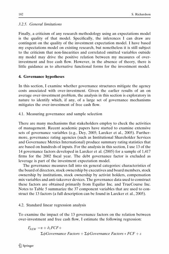
In this section, I examine whether governance structures mitigate the agencycosts associated with over-investment. Given the earlier results of an onaverage over-investment problem, the analysis in this section is exploratory innature to identify which, if any, of a large set of governance mechanismsmitigates the over-investment of free cash flow.

4.1. Measuring governance and sample selection

There are many mechanisms that stakeholders employ to check the activitiesof management. Recent academic papers have started to examine extensivesets of governance variables (e.g., Dey, 2005; Larcker et al., 2005). Further-more, governance rating agencies (such as Institutional Shareholder Servicesand Governance Metrics International) produce summary rating statistics thatare based on hundreds of inputs. For the analysis in this section, I use 13 of the14 governance factors developed in Larcker et al. (2005) for a sample of 1,417firms for the 2002 fiscal year. The debt governance factor is excluded asleverage is part of the investment expectation model.

The governance measures fall into six general categories: characteristics ofthe board of directors, stock ownership by executives and board members, stockownership by institutions, stock ownership by activist holders, compensationmix variables and anti-takeover devices. The governance data used to constructthese factors are obtained primarily from Equilar Inc. and TrueCourse Inc.Notes to Table 5 summarize the 37 component variables that are used to con-struct the 13 factors (a full description can be found in Larcker et al., 2005).

4.2. Standard linear regression analysis

To examine the impact of the 13 governance factors on the relation betweenover-investment and free cash flow, I estimate the following regression:

IeNEW ¼aþ d1FCFþ

R/Governance Factorsþ RwGovernance Factors � FCF þ e

182 S. Richardson

123

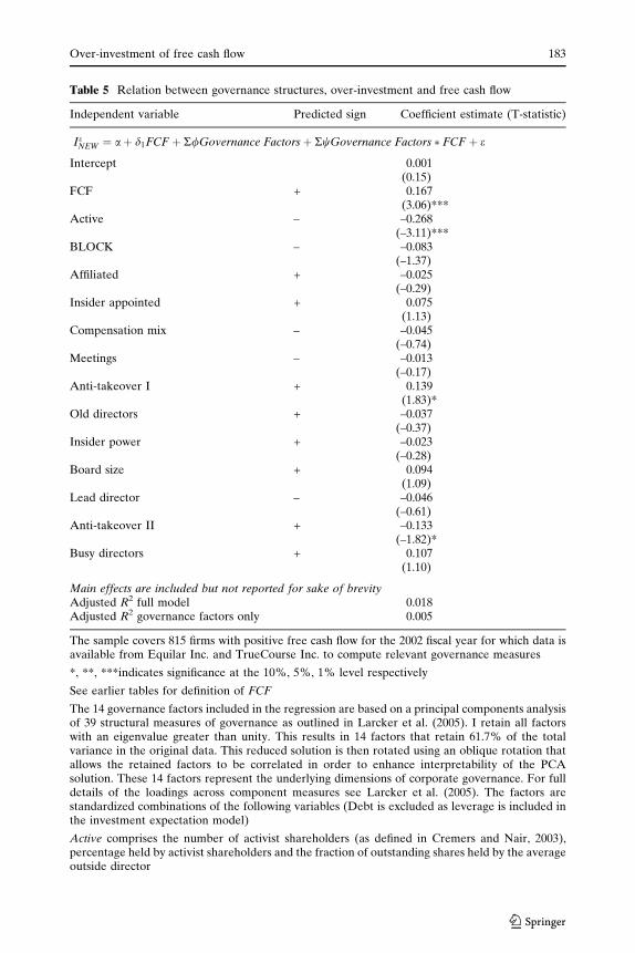
Table 5 Relation between governance structures, over-investment and free cash flow

Independent variable Predicted sign Coefficient estimate (T-statistic)

IeNEW ¼ aþ d1FCF þ R/Governance Factorsþ RwGovernance Factors � FCF þ e

Intercept 0.001(0.15)

FCF + 0.167(3.06)***

Active – –0.268(–3.11)***

BLOCK – –0.083(–1.37)

Affiliated + –0.025(–0.29)

Insider appointed + 0.075(1.13)

Compensation mix – –0.045(–0.74)

Meetings – –0.013(–0.17)

Anti-takeover I + 0.139(1.83)*

Old directors + –0.037(–0.37)

Insider power + –0.023(–0.28)

Board size + 0.094(1.09)

Lead director – –0.046(–0.61)

Anti-takeover II + –0.133(–1.82)*

Busy directors + 0.107(1.10)

Main effects are included but not reported for sake of brevityAdjusted R2 full model 0.018Adjusted R2 governance factors only 0.005

The sample covers 815 firms with positive free cash flow for the 2002 fiscal year for which data isavailable from Equilar Inc. and TrueCourse Inc. to compute relevant governance measures

*, **, ***indicates significance at the 10%, 5%, 1% level respectively

See earlier tables for definition of FCF

The 14 governance factors included in the regression are based on a principal components analysisof 39 structural measures of governance as outlined in Larcker et al. (2005). I retain all factorswith an eigenvalue greater than unity. This results in 14 factors that retain 61.7% of the totalvariance in the original data. This reduced solution is then rotated using an oblique rotation thatallows the retained factors to be correlated in order to enhance interpretability of the PCAsolution. These 14 factors represent the underlying dimensions of corporate governance. For fulldetails of the loadings across component measures see Larcker et al. (2005). The factors arestandardized combinations of the following variables (Debt is excluded as leverage is included inthe investment expectation model)

Active comprises the number of activist shareholders (as defined in Cremers and Nair, 2003),percentage held by activist shareholders and the fraction of outstanding shares held by the averageoutside director


123

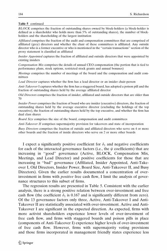
I expect a significantly positive coefficient for d1 and negative coefficientsfor each of the interacted governance factors (i.e., the w coefficients) that areincreasing in ‘‘good’’ governance (Active, BLOCK, Compensation Mix,Meetings, and Lead Director) and positive coefficients for those that areincreasing in ‘‘bad’’ governance (Affiliated, Insider Appointed, Anti-Take-over I, Old Directors, Insider Power, Board Size, Anti-Takeover II, and BusyDirectors). Given the earlier results documented a concentration of over-investment in firms with positive free cash flow, I limit the analysis of gover-nance structures to this subset of firms.

The regression results are presented in Table 5. Consistent with the earlieranalysis, there is a strong positive relation between over-investment and freecash flow (the coefficient d1 is 0.167 and is significantly different from zero).Of the 13 governance factors only three, Active, Anti-Takeover I and Anti-Takeover II are statistically associated with over-investment. Active and Anti-Takeover I are significant in the expected direction. As expected, firms withmore activist shareholders experience lower levels of over-investment offree cash fiow, and firms with staggered boards and poison pills in place(components of Anti-Takeover I) experience higher levels of over-investmentof free cash flow. However, firms with supermajority voting provisionsand those firms incorporated in management friendly states experience less

Table 5 continued

BLOCK comprises the fraction of outstanding shares owned by block-holders (a block-holder isdefined as a shareholder who holds more than 5% of outstanding shares), the number of block-holders and the shareholding of the largest institution

Affiliated comprises the fraction of the audit and compensation committees that are comprised ofaffiliated (grey) directors and whether the chair of these committees is affiliated. Any outsidedirector who is a former executive or who is mentioned in the ‘‘certain transactions’’ section of theproxy statement is classified as affiliated

Insider Appointed captures the fraction of affiliated and outside directors that were appointed byexisting insiders

Compensation Mix comprises the details of annual CEO compensation (the portion that is tied toperformance plans, stock options, restricted stock grants and annual bonuses)

Meetings comprises the number of meetings of the board and the compensation and audit com-mittees

Lead Director captures whether the firm has a lead director or an insider chair-person

Anti-Takeover I captures whether the firm has a staggered board, has adopted a poison pill and thefraction of outstanding shares held by the average affiliated director

Old Directors comprises the fraction of insider, affiliated and outside directors that are older than70

Insider Power comprises the fraction of board who are insider (executive) directors, the fraction ofoutstanding shares held by the average executive director (excluding the holdings of the topexecutive), the fraction of outstanding shares held by the top executive, and whether the firm hasdual class shares

Board Size comprises the size of the board, compensation and audit committees

Anti-Takeover II comprises supermajority provision for takeovers and state of incorporation

Busy Directors comprises the fraction of outside and affiliated directors who serve on 4 or moreother boards and the fraction of inside directors who serve on 2 or more other boards

184 S. Richardson

123

over-investment of free cash flow. Collectively, the results in Table 5 suggestthat certain governance structures are effective in mitigating the over-investment of free cash flow. However, it is important to note the very lowexplanatory power of this regression (only 2 percent of the cross-sectionalvariation in over-investment is explained jointly by free cash flow and the 13governance factors, and only 0.5% is explained solely by the governancefactors).

4.3. Additional governance analyses

The empirical analysis of governance structures and over-investmentdescribed in the last section was ex post in nature. In unreported tests, I havealso examined the link between governance structures and over-investmentfrom an ex ante perspective. Of course, finding evidence of ex post over-investment of free cash flow (as in Section 3.2) suggests that governancestructures are not designed ex ante optimally. Therefore, testing whetherthere is cross-sectional variation in governance structures as a function of thelevel of free cash flow, a measure of the propensity for over-investment, maynot be a credible null hypothesis. Nonetheless, it is instructive to examinewhether the design of governance mechanisms incorporates perceived agencycosts (as measured by the propensity of a firm to over-invest).

To examine whether governance structures are designed in response to freecash flow related agency costs, I average annual measures of free cash flow forfirms with available Compustat data for the period 1997–2002 and governancedata for the 2002 fiscal year. This leaves a sample of 1,496 firms (each firmappears only once in this analysis). Firms are sorted into portfolios based onthe magnitude of average free cash flow over the 1997–2002 period. Tests ofdifferences in governance structures across these groups are then performed.There is some evidence of different governance structures for firms with dif-ferent levels of free cash flow from earlier fiscal periods. For example, firmswith higher levels of free cash flow are more likely to have a greater con-centration of activist shareholdings, larger boards, have more incentive basedcompensation for top executives, be incorporated in shareholder friendlyregimes, and have supermajority voting provisions (all patterns are statisti-cally significant at conventional levels). Conversely, firms with higher levels offree cash flow are less likely to have affiliated directors on the board and keycommittees, and less likely to have staggered boards and poison pills (again allpatterns are statistically significant at conventional levels).

These relations, however, are not particularly strong. For example, theexplanatory power (adjusted R2) of average free cash flow from 1997 to 2002for the 13 governance factors (measured as at the end of fiscal 2002) rangedfrom –0.06% for Meetings to 15.8% for Active. Only Active, Board Size andAnti-Takeover II had an adjusted R2 greater than 2% (Adjusted R2 were 15.8,6.0 and 2.3%, respectively). Given these relative weak associations, care needsto be taken in interpreting that governance structures are designed in responseto free cash flow related agency costs. Furthermore, the data examined is


123

measured as at the end of fiscal 2002. Ideally, one would examine changes ingovernance structures through time and examine how these structures adjustin response to changes in the environment in which the firm operates (e.g.,Goodman, 2005).

The absence of a relation between free cash flow and contemporaneousgovernance structures may not be surprising given that governance structuresdo not change frequently, especially if free cash flow is not very persistent. Toaddress this issue, an alternate research design is to examine whether gover-nance structures vary based on the level of cash (industry-adjusted) reportedon the balance sheet. Even with this alternate approach, there is littleevidence of any systematic relation between governance structures and thelevel of cash held by the firm.

5. Conclusion

This paper presents evidence on firm level over-investment of free cash flow.The empirical analysis utilizes an accounting based framework to measure theconstructs of free cash flow and over-investment. A comparative advantage ofthe accounting researcher is in measuring critical constructs from the financialeconomics literature. The analysis of over-investment and free cash flow isbut one example of how accounting information can be better utilized inacademic research. The evidence in this paper suggests that over-investmentis a common problem for publicly traded US firms. For non-financial firmsduring the period 1988–2002, the average firm over-invests 20 percent of itsavailable free cash flow. Furthermore, the majority of free cash flow isretained in the form of financial assets. For each additional dollar of free cashflow the average firm in the sample retains 41 cents as either cash or mar-ketable securities. There is little evidence that free cash flow is distributed toexternal stakeholders, thereby creating the potential for retained free cashflow to be over-invested in the future. Supplemental analysis found only weakevidence that governance structures are effective in mitigating the extent ofover-investment.

These findings corroborate recent work that has found significant negativefuture stock returns from capital investment and significant growth in netoperating assets (e.g., Fairfield et al., 2003; Titman et al., 2004). Indeed, Li(2004) finds that future operating performance is lower for firms engaging ininvestment expenditure and that this negative relation is increasing in con-temporaneous free cash flow. A natural explanation for this poor futureperformance is free cash flow related agency costs.

The framework developed in the paper to measure over-investment andfree cash flow can easily be extended to consider abnormal investment moregenerally. Indeed, some recent research has started to use this framework toexamine the impact of accounting information systems on investment deci-sions and the efficient allocation of capital (e.g., Bushman, Piotroski, & Smith,2005; Goodman, 2005; Wang, 2003).

186 S. Richardson

123

Acknowledgements This paper is based on my dissertation at the University of Michigan.I would like to thank members of my dissertation committee: Richard Sloan (Chair), JerryDavis, Patricia Dechow, Doug Skinner and Matthew Shapiro. I appreciate helpful commentsfrom workshop participants at Boston College, University of California, Berkeley, University ofChicago, Columbia University, Harvard University, MIT, New York University, NorthwesternUniversity, University of Pennsylvania, University of Rochester and Stanford University, MarkBradshaw, Dan Collins, John Core, Julie Cotter, Ilia Dichev, Jef Doyle, Hulya Eraslan, RayFisman, Ted Goodman, Raffi Indjejikian, Irene Kim, David Larcker, Charles Lee (editor),Russell Lundholm, Andrew Metrick, David Musto, Venky Nagar, Stephen Penman, AbbieSmith, Gary Solon, Steve Taylor, Irem Tuna, Ross Watts, Peter Wysocki, Stephen Young, ananonymous referee and conference participants at the 2005 Review of Accounting StudiesConference, especially those of Daniel Bergstresser. I would like to recognize financial supportfrom the Paton Scholarship Fund, the Deloitte & Touche Foundation, the Arthur AndersenFoundation and the Michael J. Barrett Dissertation Award from the Institute of InternalAuditors.

References

Allen, F., & Michaely, R. (2003) Payout policy. In North-Holland handbook of economics editedby George Constantinides, Milton Harris, and Rene Stulz.

Alti, A. (2003). How sensitive is investment expenditure to cash flow when financing is friction-less? Journal of Finance, 53, 707–722.

Barro, R. (1990). The stock market and investment. Review of Financial Studies, 3, 115–131.Bates, T. W. (2005). Asset sales, investment opportunities, and the use of proceeds. Journal of

Finance, 60, 105–135.Berger, P. G., & Hann, R. (2003). The impact of SFAS 131 on Information and Monitoring.

Journal of Accounting Research, 41, 163–223.Blanchard, O. J., Lopez-de-Silanes, F., & Shleifer, A. (1994). What do firms do with cash wind-

falls? Journal of Financial Economics, 36, 337–360.Brown, L., & Caylor, M. (2004). Corporate Governance and Firm Performance. Working paper,

Georgia State University.Bushman, R. M., Piotroski, J. D., & Smith, A. J. (2005). Capital allocation and timely recognition

of economic losses: International evidence. Working paper, University of Chicago.DeAngelo, H., DeAngelo, L., & Stulz, R. (2004). Dividend Policy, Agency Costs and Earned

Equity. Working paper, University of Southern California.Dechow, P. M., Hutton, A. P., & Sloan, R. G. (1999). An empirical assessment of the residual

income valuation model. Journal of Accounting and Economics, 26, 1–34.Dechow, P. M., Richardson, S. A., & Sloan, R. G. (2005). The Persistence and Pricing of the Cash

Component of Earnings. Working paper, University of Michigan and University of Pennsyl-vania.

Dey, A. (2005). Corporate governance and financial reporting credibility. Working paper,Northwestern University.

Fairfield, P. M. (1994). P/E, P/B and the present value of future dividends. Financial AnalysisJournal, July–Aug, 23–31

Fairfield, P. M., Whisenant, J. S., & Yohn, T. L. (2003). Accrued earnings and growth: Implicationsfor future profitability and market mispricing. Accounting Review, 78, 353–371.

Fama, E. F., & French, K. R. (1997). Industry costs of equity. Journal of Financial Economics, 43,153–194

Fama, E. F., & Macbeth, J. D. (1973). Risk, return and equilibrium—empirical tests. The Journalof Political Economy, 81, 607–636

Fazzari, S. M., Hubbard, R. G., & Petersen, B. C. (1988). Financing constraints on corporateinvestment. Brookings Papers on Economic Activity, 141–195.

Fazzari, S. M., & Petersen, B. C. (1993). Working capital and fixed investment: New evidence onfinancing constraints. RAND Journal of Economics, 24, 328–342.

Feltham, G. A., & Ohlson, J. A. (1996). Uncertainty resolution and the theory of depreciationmeasurement. Journal of Accounting Research, 34, 209–234.


123

Gompers, P. A., Ishii, J. L., & Metrick, A. (2003). Corporate Governance and Equity Prices.Quarterly Journal of Economics, 118, 107–155.

Goodman, T. H. (2005). How do contracts adapt to an increase in free cash flow? Working paper,University of Pennsylvania.

Harford, J. (1999). Corporate cash reserves and acquisitions. Journal of Finance, 54, 1969–1997.Hoshi, T., Kashyap, A., & Scharfstein, D. (1991). Corporate structure, liquidity and investment:

Evidence from Japanese industrial groups. Quarterly Journal of Economics, 106, 33–60.Hubbard, R. G. (1998). Capital-market imperfections and investment. Journal of Economic Lit-

erature, 36, 193–225.Iman, R. L., & Conover, W. J. (1979). The use of rank transform in regression. Technometrics, 21,

499–509.Jensen, M. C. (1986). Agency costs and free cash flow, corporate finance and takeovers. American

Economic Review, 76, 659–665.Jensen, M. C., & Meckling, W. H. (1976). Theory of the firm: Managerial behavior, agency costs

and ownership structure. Journal of Financial Economics, 3, 305–360.Kaplan, S. N., & Zingales, L. (1997). Do investment-cash flow sensitivities provide useful

measures of financing constraints? Quarterly Journal of Economics, 112, 169–215Kaplan, S. N., & Zingales, L. (2000). Investment-cash flow sensitivities are not valid measures of

financing constraints. Quarterly Journal of Economics, 115, 707–712.Lamont, O. (1997). Cash flow and investment: Evidence from internal capital markets. Journal of

Finance, 52, 83–109.Lamont, O. (2000). Investment plans and stock returns. Journal of Finance, 55, 2719–2748.Lang, L. H. P., Stulz, R. M., & Walkling, R. A. (1991). A test of the free cash flow hypothesis: The

case of bidder returns. Journal of Financial Economics, 29, 315–335Larcker, D. F., Richardson, S. A. & Tuna, A. I. (2005). How important is corporate governance?

Working paper, University of Pennsylvania.Li, D. (2004). The implications of capital investments for future profitability and stock returns—an

overinvestment perspective. Working paper, University of California, Berkeley.Modigliani, F., & Miller, M. (1958). The cost of capital, corporation finance and the theory of

investment. American Economic Review, 48, 261–297.Morck, R., Shleifer, A., & Vishny, R. W. (1990). Do managerial objectives drive bad acquisitions?

Journal of Finance, 45, 31–48.Myers, S. C. (1977). Determinants of corporate borrowing. Journal of Financial Economics, 5,

147–175.Myers, S. C., & Majluf, N. (1984). Corporate financing and investment decisions when firms have

investment information that investors do not have. Journal of Financial Economics, 13, 187–220.Ohlson, J. A. (1995). Earnings, book values and dividends in security valuation. Contemporary

Accounting Research, 11, 661–687.Opler, T., Pinkowitz, L., Stulz, R., & Williamson, R. (1999). The determinants and implications of

corporate cash holdings. Journal of Financial Economics, 52, 3–46.Opler, T., Pinkowitz, L., Stulz, R., & Williamson, R. (2001). Corporate cash holdings. Journal of

Applied Corporate Finance, 14, 55–66.Opler, T., & Titman, S. (1993). The determinants of leveraged buyout activity: Free cash flow vs.

financial distress costs. The Journal of Finance, 48, 1985–1999.Penman, S. H. (1991). An evaluation of accounting rate of return. Journal of Accounting, Auditing

and Finance Spring, 6, 233–255Penman, S. H. (1996). The articulation of price-earnings ratios and market-to-book ratios and the

evaluation of growth. Journal of Accounting Research, 34, 235–259.Rogers, W. (1993). Regression standard errors in clustered samples. Stata technical bulletin rep-

rints (vol. 3, pp. 83–94). College Station, Texas: Stata Press.Shleifer, A., & Vishny, R. W. (1997). A survey of corporate governance. Journal of Finance, 52(2),

737–783.Sloan, R. G. (1996). Do stock prices fully reflect information in accruals and cash flows about

future earnings? The Accounting Review, 71, 289–315.

188 S. Richardson

123

Strong, J. S., & Meyer, J. R. (1990). Sustaining Investment, discretionary investment, and valu-ation: A residual funds study of the paper industry. In R. G. Hubbard (ed.) Asymmetricinformation, corporate finance, and investment (pp. 127–148). Chicago, IL: University ofChicago Press.

Stulz, R. M. (1990). Managerial discretion and optimal financing policies. Journal of FinancialEconomics, 26, 3–27.

Titman, S., Wei, K. C. J., & Xie, F. (2004). Capital investments and stock returns. Journal ofFinancial and Quantitative Analysis, 39, 677–700.

Wang, X. (2003). Capital allocation and accounting information properties. Working paper,Emory University.

White, H. (1980). A Heteroskedasticity-consistent covariance matrix estimator and a direct testfor heteroskedasticity. Econometrica, 48, 817–838.

Whited, T. (1992). Debt, liquidity constraints and corporate investment: Evidence from paneldata. Journal of Finance, 47, 1425–1460.

Wilcox, J. (1984). The P/B-ROE valuation model. Financial Analysts Journal, Jan–Feb, 58–66.


123

Rast Richardson

Documents

Transcript of Rast Richardson