Ranking Games - Technische Universität...

Ranking Games

Felix Brandt a,∗ Felix Fischer a Paul Harrenstein a

Yoav Shoham b

aInstitut fur Informatik, Universitat MunchenOettingenstr. 67, 80538 Munchen, Germany

bComputer Science Department, Stanford University353 Serra Mall, Stanford CA 94305, USA

Abstract

The outcomes of many strategic situations such as parlor games or competitive economicscenarios are rankings of the participants, with higher ranks generally at least as desirableas lower ranks. Here we define ranking games as a class of n-player normal-form gameswith a payoff structure reflecting the players’ von Neumann-Morgenstern preferences overtheir individual ranks. We investigate the computational complexity of a variety of com-mon game-theoretic solution concepts in ranking games and deliver hardness results foriterated weak dominance and mixed Nash equilibrium when there are more than two play-ers, and for pure Nash equilibrium when the number of players is unbounded but the gameis described succinctly. This dashes hope that multi-player ranking games can be solvedefficiently, despite their profound structural restrictions. Based on these findings, we pro-vide matching upper and lower bounds for three comparative ratios, each of which relatestwo different solution concepts: the price of cautiousness, the mediation value, and theenforcement value.

Keywords: Multi-Agent Systems, Game Theory, Strict Competitiveness, n-Player Games,Solution Concepts, Computational Complexity

1 Introduction

The situations studied by the theory of games may involve different levels of antag-onism. On the one end of the spectrum are games of pure coordination, on the other

∗ Corresponding author; Telephone: +49 89 2180 9406; Fax: +49 89 2180 9338Email addresses: [email protected] (Felix Brandt),[email protected] (Felix Fischer), [email protected] (PaulHarrenstein), [email protected] (Yoav Shoham).

Preprint submitted to Elsevier 28 August 2008

those in which the players’ interests are diametrically opposed. In this paper, we putforward a new class of competitive multi-player games whose outcomes are rank-ings of the players, i.e., orderings of the players representing how well they havedone in the game relative to one another. We assume players to weakly prefer ahigher rank over a lower one and to be indifferent as to the other players’ ranks.This type of situation is commonly encountered in parlor games, competitions,patent races, competitive resource allocation domains, social choice settings, orany other strategic situation where players are merely interested in performing op-timal relative to their opponents rather than in absolute measures. Formally, rankinggames are defined as normal-form games in which the payoff function representsthe players’ von Neumann-Morgenstern preferences over lotteries over rankings. Anoteworthy special case of particular relevance to game playing in AI are single-winner games where in any outcome one player wins and all others lose.

While two-player ranking games form a subclass of zero-sum games, no such rela-tionship holds for ranking games with more than two players. Moreover, whereasthe notion of a ranking is most natural in multi-player settings, this seems to beless so for the requirement that the sum of payoffs in all outcomes be constant, asany game can be transformed into a constant-sum game by merely introducing anadditional player (with only one action at his disposal) who absorbs the payoffs ofthe other players (von Neumann and Morgenstern, 1947).

As with games in which both contrary and common interests prevail, it turns outthat solving ranking games tends to become considerably more complicated as soonas more than two players are involved. The maximin solution does not unequivo-cally extend to general n-player games and numerous alternate solution conceptshave been proposed to cope with this type of situation. None of them, however,seems to be as compelling as maximin is for two-player zero-sum games. In thispaper we study and compare the properties of a variety of solution concepts inranking games. The results of this paper fall into two different categories. First,we investigate the complexity of a number of computational problems related tocommon solution concepts in ranking games, particularly Nash equilibrium anditerated weak dominance. Second, we study a number of comparative ratios inranking games, each of which relates two different solution concepts: the price ofcautiousness, the mediation value, and the enforcement value.

The computational effort required to determine a solution is obviously a very im-portant property of any solution concept. If computing a solution is intractable, thesolution concept is rendered virtually useless for large problem instances that donot exhibit additional structure. The importance of this aspect has by no means es-caped the attention of game theorists. In an interview with Eric van Damme (1998),Robert Aumann claimed: “My own viewpoint is that, inter alia, a solution conceptmust be calculable, otherwise you are not going to use it.” It has subsequently beenargued that this still holds if one subscribes to a purely descriptive view of solutionconcepts: “I believe that the complexity of equilibria is of fundamental importance

2

in game theory, and not just a computer scientist’s afterthought. Intractability of anequilibrium concept would make it implausible as a model of behavior” (Papadim-itriou, 2005). In computational complexity theory, the distinction between tractableand intractable problems is typically one between membership in the class P ofproblems that can be solved in time polynomial in the size of the problem instanceversus hardness for the class NP of problems a solution of which can be verifiedefficiently. A third class that will play an important role in the context of this paperis PPAD. Problems in PPAD are guaranteed to possess a solution, and emphasis isput on actually finding it. Given the current state of complexity theory, we cannotprove the actual intractability of most algorithmic problems, but merely give evi-dence for their intractability. NP-hardness of a problem is commonly regarded asvery strong evidence against computational tractability because it relates the prob-lem to a large class of problems for which no efficient algorithm is known, despiteenormous efforts to find such algorithms. To some extent, the same reasoning canalso be applied to PPAD-hardness.

We study the computational complexity of common game-theoretic solution con-cepts in ranking games and deliver NP-hardness and PPAD-hardness results, re-spectively, for iterated weak dominance and (mixed) Nash equilibria when thereare more than two players, and an NP-hardness result for pure Nash equilibria ingames with an unbounded number of players. This dashes hope that multi-playerranking games can be solved efficiently, despite their profound structural restric-tions. Remarkably, all hardness results hold for arbitrary preferences over ranks,provided they meet the requirements listed above. Accordingly, even very restrictedsubclasses of ranking games such as single-winner games—in which players onlycare about winning—or single-loser games—in which players merely wish not tobe ranked last—are computationally hard to solve.

By contrast, maximin strategies (von Neumann, 1928) as well as correlated equilib-ria (Aumann, 1974) are known to be computationally easy via linear programmingfor any class of games. Against the potency of these concepts, however, other ob-jections can be brought in. Playing a maximin strategy is extremely defensive and aplayer may have to forfeit a considerable amount of payoff in order to guarantee hissecurity level. Correlation, on the other hand, may not be feasible in all practicalapplications, and may fail to provide an improvement of social welfare in restrictedclasses of games (Moulin and Vial, 1978). Thus, we come to consider the follow-ing comparative ratios in an effort to facilitate the quantitative analysis of solutionconcepts in ranking games:

• the price of cautiousness, i.e., the ratio between an agent’s minimum payoff in aNash equilibrium and his security level

• the mediation value, i.e., the ratio between the social welfare obtainable in thebest correlated equilibrium vs. the best Nash equilibrium, and

• the enforcement value, i.e., the ratio between the highest obtainable social wel-fare and that of the best correlated equilibrium.

3

Each of these values obviously equals 1 in the case of two-player ranking games, asthese form a subclass of constant-sum games. Accordingly, the interesting questionto ask concerns the bounds of these values for ranking games with more than twoplayers.

2 Introductory Example

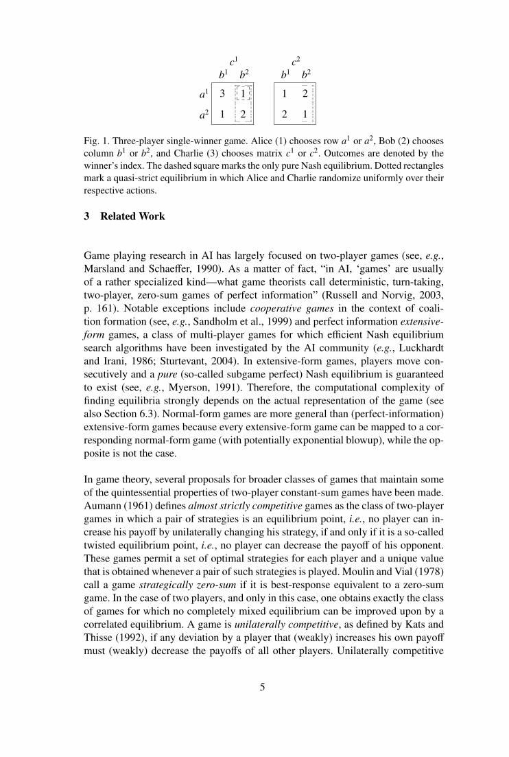
To illustrate the issues addressed in this paper, consider a situation in which Alice,Bob, and Charlie are to choose a winner from among themselves by means of thefollowing protocol. Each of them is either to raise or not to raise their hand; they areto do so simultaneously and independently of one another. Alice wins if the numberof hands raised, including her own, is odd, whereas Bob is victorious if this num-ber equals two. Should nobody raise their hand, Charlie wins. The normal-form ofthis game is shown in Figure 1. What course of action would you recommend toAlice? There is a Nash equilibrium in which Alice raises her hand, another one inwhich she does not raise her hand, and still another one in which she randomizesuniformly between these two options. In the only pure, i.e., non-randomized, equi-librium of the game, Alice does not raise her hand. If the latter were to occur, wemust assume that Alice believes that Bob will raise his hand and Charlie will not.This assumption, however, is unreasonably strong as no such beliefs can be derivedfrom the mere description of the game. Moreover, both Bob and Charlie may de-viate from their respective strategies to any other strategy without decreasing theirchances of winning. After all, they cannot do any worse than losing.

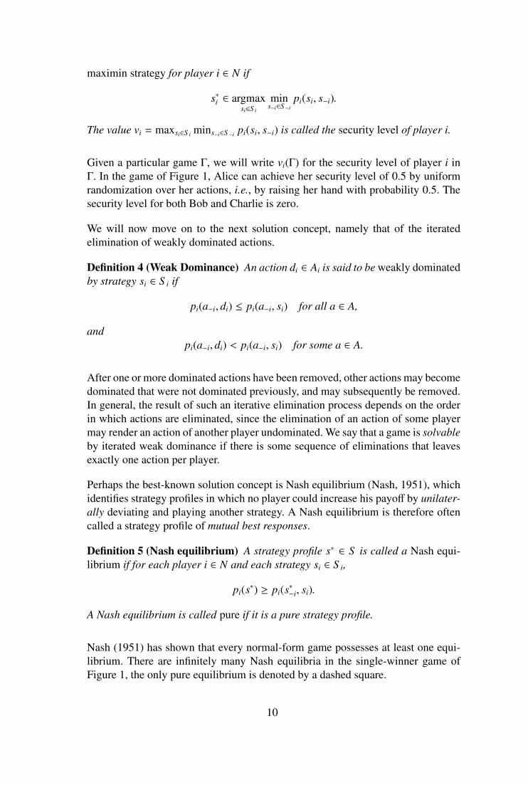
This points at a weakness of pure Nash equilibrium as a solution concept inherentin ranking games, since in any outcome some player has to be ranked last. On theother hand, it is very well possible that all the actions in the support of a mixedequilibrium yield each player a strictly higher expected payoff than any action notin the support, mitigating the phenomenon mentioned above. In other words, suchequilibria can be quasi-strict, a property no pure equilibrium in a ranking gamehas. While quasi-strict equilibria may fail to exist in ranking games with morethan two players (see Figure 4), we conjecture, and prove for certain sub-cases,that every single-winner game possesses at least one non-pure equilibrium, i.e., anequilibrium where at least one player randomizes. We note without proof that thisproperty fails to hold for general ranking games.

Returning to our example, it is unclear which strategy would maximize Alice’schances of winning. By playing her maximin strategy, Alice can guarantee a par-ticular probability of winning, her so-called security level, no matter which actionsher opponents choose. Alice’s security level in this particular game is 0.5 and canbe obtained by randomizing uniformly between both actions. The same expectedpayoff is achieved in the worst quasi-strict equilibrium of the game where Alice andCharlie randomize uniformly and Bob invariably raises his hand (see Figure 1).

4

a1

a2

b1 b2 b1 b2c1 c2

3

1

1

2

1

2

2

1

Fig. 1. Three-player single-winner game. Alice (1) chooses row a1 or a2, Bob (2) choosescolumn b1 or b2, and Charlie (3) chooses matrix c1 or c2. Outcomes are denoted by thewinner’s index. The dashed square marks the only pure Nash equilibrium. Dotted rectanglesmark a quasi-strict equilibrium in which Alice and Charlie randomize uniformly over theirrespective actions.

3 Related Work

Game playing research in AI has largely focused on two-player games (see, e.g.,Marsland and Schaeffer, 1990). As a matter of fact, “in AI, ‘games’ are usuallyof a rather specialized kind—what game theorists call deterministic, turn-taking,two-player, zero-sum games of perfect information” (Russell and Norvig, 2003,p. 161). Notable exceptions include cooperative games in the context of coali-tion formation (see, e.g., Sandholm et al., 1999) and perfect information extensive-form games, a class of multi-player games for which efficient Nash equilibriumsearch algorithms have been investigated by the AI community (e.g., Luckhardtand Irani, 1986; Sturtevant, 2004). In extensive-form games, players move con-secutively and a pure (so-called subgame perfect) Nash equilibrium is guaranteedto exist (see, e.g., Myerson, 1991). Therefore, the computational complexity offinding equilibria strongly depends on the actual representation of the game (seealso Section 6.3). Normal-form games are more general than (perfect-information)extensive-form games because every extensive-form game can be mapped to a cor-responding normal-form game (with potentially exponential blowup), while the op-posite is not the case.

In game theory, several proposals for broader classes of games that maintain someof the quintessential properties of two-player constant-sum games have been made.Aumann (1961) defines almost strictly competitive games as the class of two-playergames in which a pair of strategies is an equilibrium point, i.e., no player can in-crease his payoff by unilaterally changing his strategy, if and only if it is a so-calledtwisted equilibrium point, i.e., no player can decrease the payoff of his opponent.These games permit a set of optimal strategies for each player and a unique valuethat is obtained whenever a pair of such strategies is played. Moulin and Vial (1978)call a game strategically zero-sum if it is best-response equivalent to a zero-sumgame. In the case of two players, and only in this case, one obtains exactly the classof games for which no completely mixed equilibrium can be improved upon by acorrelated equilibrium. A game is unilaterally competitive, as defined by Kats andThisse (1992), if any deviation by a player that (weakly) increases his own payoff

must (weakly) decrease the payoffs of all other players. Unilaterally competitive

5

games retain several interesting properties of two-player constant-sum games inthe n-player case: all equilibria yield the same payoffs, equilibrium strategies areinterchangeable, and, the set of equilibria is convex provided that some mild condi-tions hold. It was later shown by Wolf (1999) that pure Nash equilibria of n-playerunilaterally competitive games are always profiles of maximin strategies. Whenthere are just two players, all of the above classes contain constant-sum games andthus two-player ranking games. Neither is contained in the other in the n-playercase. The notion of competitiveness as embodied in ranking games is remotely re-lated to spitefulness (Morgan et al., 2003; Brandt et al., 2007), where agents aim atmaximizing their payoff relative to the payoff of all other agents.

Most work on comparative ratios in game theory has been inspired by the litera-ture on the price of anarchy (Koutsoupias and Papadimitriou, 1999; Roughgarden,2005), i.e., the ratio between the highest obtainable social welfare and that of thebest Nash equilibrium. Similar ratios for correlated equilibria, the value of medi-ation, i.e., the ratio between the social welfare obtainable in the best correlatedequilibrium vs. the best Nash equilibrium and the enforcement value, i.e., the ratiobetween the highest obtainable social welfare and that of the best correlated equi-librium, were introduced by Ashlagi et al. (2005). It is known that the mediationvalue of strategically zero-sum games is 1 and that of almost strictly competitivegames is greater than 1, showing that correlation can be beneficial even in gamesof strict antagonism (Raghavan, 2002). To the best of our knowledge, Tennenholtz(2002) was the first to conduct a quantitative comparison of Nash equilibrium pay-offs and security levels. This work is inspired by an intriguing example game dueto Aumann (1985), in which the only Nash equilibrium yields each player no morethan his security level although the equilibrium strategies are different from themaximin strategies. In other words, the equilibrium strategies yield security levelpayoffs without guaranteeing them.

4 The Model

A game form is a quadruple (N, (Ai)i∈N ,Ω, g), where N is a finite non-empty set ofplayers, Ai a finite and non-empty set of actions available to player i, Ω a set ofoutcomes, and g :

i∈N Ai → Ω an outcome function mapping each action profile

to an outcome in Ω. The set

i∈N Ai of action profiles is denoted by A. We assumethat each player entertain preferences over lotteries over Ω that comply with the vonNeumann-Morgenstern axioms (von Neumann and Morgenstern, 1947). Thus, thepreferences of each player i can be represented by a real valued payoff function pi

on Ω. We arrive at the following definition of a normal-form game.

Definition 1 (Game in normal form) A game in normal form Γ is given by a quin-tuple (N, (Ai)i∈N ,Ω, g, (pi)i∈N) where (N, (Ai)i∈N ,Ω, g) is a game form and eachpi : Ω→ R is a real valued payoff function.

6

We generally assume the payoff functions pi to be extended so as to apply directlyto action profiles a ∈ A by setting pi(a) = pi(g(a)).

We say a game is rational if for all i ∈ N and all a ∈ A, pi(a) ∈ Q. A game is binaryif for all i ∈ N and all a ∈ A, pi(a) ∈ 0, 1. A game with two players will also bereferred to as a bimatrix game. Unless stated otherwise, we will henceforth assumethat every player has at least two actions. Subscripts will be used to identify theplayer to which an action belongs, superscripts to index the actions of a particularplayer. For example, we write ai for a typical action of player i and a j

i for hisjth action. For better readability, we also use lower case roman letters from thebeginning of the alphabet to denote the players’ actions in such a way that a j = a j

1,b j = a j

2, c j = a j3, and so forth.

The concept of an action profile can be generalized to that of a mixed strategy pro-file by letting players randomize over their actions. We have S i denote the set ∆(Ai)of probability distributions over player i’s actions, the mixed strategies availableto player i, and S the set

i∈N S i of mixed strategy profiles with s as typical el-

ement. Payoff functions naturally extend to mixed strategy profiles, and we willfrequently write pi(s) for the expected payoff of player i, and p(s) for the socialwelfare

∑i∈N pi(s) under the strategy profile s. We have n stand for the number

|N | of players. In the following, A−i and S −i denote the set of action profiles forall players but i and the set of strategy profiles for all players but i, respectively.We use si for the ith strategy in profile s and s−i for the vector of all strategies ins but si. Furthermore, s(ai) and si(ai) stand for the probability player i assigns toaction ai in strategy profile s or strategy si, respectively. The pure strategy si suchthat si(ai) = 1 we also denote by ai whenever this causes no confusion. Moreover,we use (s−i, ti) to refer to the strategy profile obtained from s by replacing si by ti.For better readability we usually avoid double parentheses and write, e.g., p(s−i, ti)instead of p((s−i, ti)).

4.1 Rankings and Ranking Games

A ranking game is a normal-form game whose outcomes are rankings of its play-ers. A ranking indicates how well each player has done relative to the other play-ers in the game. Formally, a ranking r = [r1, . . . , rn] is an ordering of the playersin N in which player r1 is ranked first, player r2 ranked second, and so forth, withplayer rn ranked last. Obviously, this limits the number of possible outcomes to n!irrespective of the the number of actions the players have at their disposal. The setof rankings over a set N of players we denote by RN . A game form (N, (Ai)i∈N ,Ω, g)is a ranking game form if the set of outcomes is given by the set of rankings of theplayers, i.e., if Ω = RN .

We assume that all players weakly prefer higher ranks over lower ranks, and strictly

7

prefer being ranked first to being ranked last. Furthermore, each player is assumedto be indifferent as to the ranks of the other players. Even so, a player may prefer tobe ranked second for certain to having a fifty-fifty chance of being ranked first orbeing ranked third, whereas other players may judge quite differently. Accordingly,we have a rank payoff function pi : RN → R represent player i’s von Neumann-Morgenstern preferences over lotteries over RN . For technical convenience, we nor-malize the payoffs to the unit interval [0, 1]. Formally, a rank payoff function pi

over RN satisfies the following three conditions for all rankings r, r′ ∈ RN:

(i) pi(r) ≥ pi(r′), if rk = r′m = i and k ≤ m,(ii) pi(r) = 1, if i = r1, and

(iii) pi(r) = 0, if i = rn.

We are now in a position to formally define the concept of a ranking game.

Definition 2 (Ranking game) A normal form game Γ = (N, (Ai)i∈N ,Ω, g, (pi)i∈N)is a ranking game if Ω is the set RN of rankings over N and each pi : RN → R is arank payoff function over RN .

Condition (i) above implies that a player’s payoff for a ranking r only depends onthe rank assigned to him in r. Accordingly, for 1 ≤ k ≤ n, we have pk

i denote theunique payoff player i obtains in any ranking r in which i is ranked kth. The rankpayoff function of player i can then conveniently and compactly be represented byhis rank payoff vector ~pi = (p1

i , . . . , pni ).

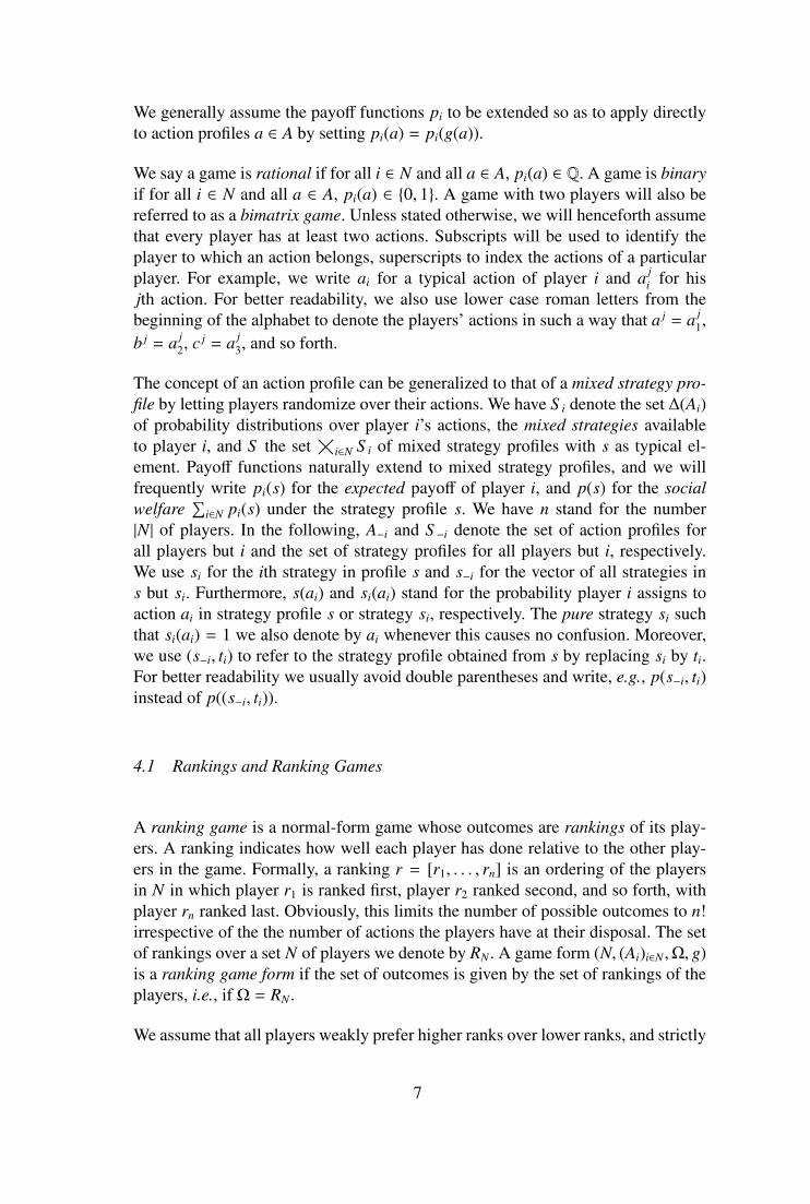
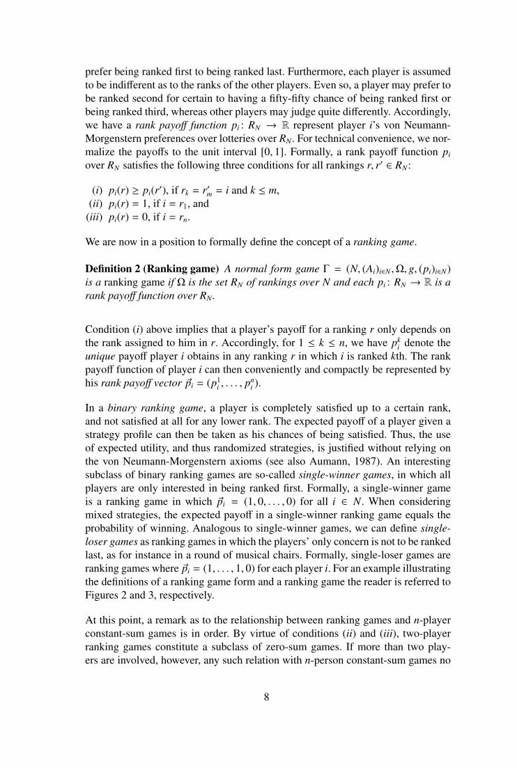
In a binary ranking game, a player is completely satisfied up to a certain rank,and not satisfied at all for any lower rank. The expected payoff of a player given astrategy profile can then be taken as his chances of being satisfied. Thus, the useof expected utility, and thus randomized strategies, is justified without relying onthe von Neumann-Morgenstern axioms (see also Aumann, 1987). An interestingsubclass of binary ranking games are so-called single-winner games, in which allplayers are only interested in being ranked first. Formally, a single-winner gameis a ranking game in which ~pi = (1, 0, . . . , 0) for all i ∈ N. When consideringmixed strategies, the expected payoff in a single-winner ranking game equals theprobability of winning. Analogous to single-winner games, we can define single-loser games as ranking games in which the players’ only concern is not to be rankedlast, as for instance in a round of musical chairs. Formally, single-loser games areranking games where ~pi = (1, . . . , 1, 0) for each player i. For an example illustratingthe definitions of a ranking game form and a ranking game the reader is referred toFigures 2 and 3, respectively.

At this point, a remark as to the relationship between ranking games and n-playerconstant-sum games is in order. By virtue of conditions (ii) and (iii), two-playerranking games constitute a subclass of zero-sum games. If more than two play-ers are involved, however, any such relation with n-person constant-sum games no

8

c1

b1 b2

a1 [1, 3, 2] [2, 1, 3]

a2 [2, 3, 1] [3, 2, 1]

c2

b1 b2

[3, 2, 1] [3, 1, 2]

[2, 1, 3] [1, 3, 2]

Fig. 2. A 2 × 2 × 2 ranking game form. One player chooses rows, another columns, anda third matrices. Each combination of actions results in a ranking. For example, actionprofile (a2, b2, c2) leads to the row player 1 being ranked first, the matrix player 3 secondand the column player 2 third.

c1

b1 b2

a1 (1, 0, 1) ( 12 , 1, 0)

a2 (0, 1, 1) (0, 0, 1)

c2

b1 b2

(0, 0, 1) ( 12 , 0, 1)

( 12 , 1, 0) (1, 0, 1)

Fig. 3. A ranking game associated with the ranking game form depicted in Figure 2. Therank payoff for the three players are given by ~p1 = (1, 1

2 , 0), ~p2 = (1, 0, 0) and ~p3 = (1, 1, 0).

longer holds. A strategic game can be converted to a zero-sum game via positiveaffine transformations only if all outcomes of the game lie on an (n−1)-dimensionalhyperplane in the n-dimensional outcome space. Clearly, there are ranking games(with non-identical rank payoff vectors and more than two players) for which thisis not the case. For example, consider a three-player ranking game with rank pay-off vectors ~p1 = ~p2 = (1, 0, 0) and ~p3 = (1, 1, 0) that has among its outcomes therankings [1, 2, 3], [2, 1, 3], [3, 1, 2], and [1, 3, 2]. As a consequence, ranking gamesare no subclass of (the games that can be transformed into) constant-sum games. Itis readily appreciated that the opposite inclusion does not hold either.

5 Solution Concepts

In this section we review a number of well-known solution concepts and provesome properties specific to ranking games.

On a normative interpretation, the solution concepts game theory has producedidentify reasonable, desirable, or otherwise significant strategy profiles in games.Perhaps the most cautious way for a player to proceed is to ensure his security levelby playing his maximin strategy, the strategy that maximizes his payoff in case theother players were to conspire against him and try to minimize his payoff.

Definition 3 (Maximin strategy and security level) A strategy s∗i ∈ S i is called a

9

maximin strategy for player i ∈ N if

s∗i ∈ argmaxsi∈S i

mins−i∈S −i

pi(si, s−i).

The value vi = maxsi∈S i mins−i∈S −i pi(si, s−i) is called the security level of player i.

Given a particular game Γ, we will write vi(Γ) for the security level of player i inΓ. In the game of Figure 1, Alice can achieve her security level of 0.5 by uniformrandomization over her actions, i.e., by raising her hand with probability 0.5. Thesecurity level for both Bob and Charlie is zero.

We will now move on to the next solution concept, namely that of the iteratedelimination of weakly dominated actions.

Definition 4 (Weak Dominance) An action di ∈ Ai is said to be weakly dominatedby strategy si ∈ S i if

pi(a−i, di) ≤ pi(a−i, si) for all a ∈ A,

andpi(a−i, di) < pi(a−i, si) for some a ∈ A.

After one or more dominated actions have been removed, other actions may becomedominated that were not dominated previously, and may subsequently be removed.In general, the result of such an iterative elimination process depends on the orderin which actions are eliminated, since the elimination of an action of some playermay render an action of another player undominated. We say that a game is solvableby iterated weak dominance if there is some sequence of eliminations that leavesexactly one action per player.

Perhaps the best-known solution concept is Nash equilibrium (Nash, 1951), whichidentifies strategy profiles in which no player could increase his payoff by unilater-ally deviating and playing another strategy. A Nash equilibrium is therefore oftencalled a strategy profile of mutual best responses.

Definition 5 (Nash equilibrium) A strategy profile s∗ ∈ S is called a Nash equi-librium if for each player i ∈ N and each strategy si ∈ S i,

pi(s∗) ≥ pi(s∗−i, si).

A Nash equilibrium is called pure if it is a pure strategy profile.

Nash (1951) has shown that every normal-form game possesses at least one equi-librium. There are infinitely many Nash equilibria in the single-winner game ofFigure 1, the only pure equilibrium is denoted by a dashed square.

10

a1

a2

b1 b2 b1 b2c1 c2

2

1

1

2

3

1

1

1

Fig. 4. Three-player single-winner game without quasi-strict equilibria. Dashed boxes markall Nash equilibria (one player may mix arbitrarily in boxes that span two outcomes).

A weakness of Nash equilibrium as a normative solution concept is that, given par-ticular strategies of the other players, a player may be indifferent between an actionhe plays with non-zero probability and an action he does not play at all. For exam-ple, in the pure Nash equilibrium of the game in Figure 1, players 2 and 3 mightjust as well play any other strategy without decreasing their chances of winning. Toalleviate the effects of this phenomenon, Harsanyi (1973) proposed to impose theadditional requirement that every best response be played with positive probability.Any Nash equilibrium that also satisfies this latter restriction is called a quasi-strictequilibrium. 1

Definition 6 (Quasi-strict equilibrium) A Nash equilibrium s∗ ∈ S is calledquasi-strict equilibrium if for all i ∈ N and all ai, a′i ∈ Ai with s∗(ai) > 0 ands∗(a′i) = 0,

pi(s∗−i, ai) > pi(s∗−i, a′i).

Figure 1 shows a quasi-strict equilibrium of the game among Alice, Bob and Char-lie. 2 While quasi-strict equilibria have been shown to always exist in two-playergames (Norde, 1999), this is not generally the case for games with more than twoplayers. Figure 4 shows that quasi-strict equilibria need not even exist in single-winner games. 3

In ranking games, the stability of some Nash equilibria is especially questionablebecause they prescribe losing players to play certain strategies even though theycould just as well play any other strategy without a chance of decreasing their pay-off. In each outcome of a ranking game, there is at least one player that is rankedlowest and accordingly receives the minimum payoff of zero. Consequently, anysuch player has no incentive to actually play the action prescribed by the Nash

1 Harsanyi originally referred to quasi-strict equilibrium as “quasi-strong”. However, thisterm has been dropped to distinguish the concept from Aumann’s strong equilibrium (Au-mann, 1959).2 Observe that Charlie plays a weakly dominated action with positive probability in thisequilibrium.3 There are only few examples in the literature for games without quasi-strict equilibria(essentially there is one example by van Damme (1983) and another one by Cubitt andSugden (1994)). For this reason, the game depicted in Figure 4 might be of independentinterest.

11

equilibrium. It follows that all pure equilibria are weak in this sense. This problemis especially urgent in single-winner games, where all players but the winner are in-different over which action to play. Quasi-strict equilibrium can be used to formallyillustrate this weakness.

Fact 1 Quasi-strict equilibria in ranking games are never pure, i.e., in any quasi-strict equilibrium there is at least one player who randomizes over some of hisactions.

Although ranking games may have pure Nash equilibria, it seems as if most ofthem possess non-pure equilibria as well, i.e., mixed strategy equilibria where atleast one player randomizes. We prove this claim for three subclasses of rankinggames.

Theorem 1 The following classes of ranking games always possess at least onenon-pure equilibrium:

(i) two-player ranking games,(ii) three-player single-winner games where each player has two actions, and

(iii) n-player single-winner games where the security level of at least two playersis positive.

Proof: Statement (i) follows from Fact 1 and the existence result by Norde (1999).For reasons of completeness, we give a simple alternative proof. Assume for con-tradiction that there is a two-player ranking game that only possesses pure equi-libria and consider, without loss of generality, a pure equilibrium s∗ in whichplayer 1 wins. Since player 2 must be incapable of increasing his payoff by deviat-ing from s∗, player 1 has to win no matter which action the second player chooses.As a consequence, the strategies in s∗ remain in equilibrium even if player 2’s strat-egy is replaced with an arbitrary randomization among his actions.

As for (ii), consider a three-player single winner game with actions A1 = a1, a2,A2 = b1, b2, and A3 = c1, c2. Assume for contradiction that there are only pureequilibria in the game and consider, without loss of generality, a pure equilibriums∗ = (a1, b1, c1) in which player 1 wins. In the following, we say that a pure equi-librium is semi-strict if at least one player strictly prefers his equilibrium actionover all his other actions given that the other players play their equilibrium actions.In single-winner games, this player has to be the winner in the pure equilibrium.We first show that if s∗ is semi-strict, i.e., player 1 does not win in action pro-file (a2, b1, c1), then there must exist a non-pure equilibrium. For this, consider thestrategy profile s1 = (a1, s1

2, c1), where s1

2 is the uniform mixture of player 2’s ac-tions b1 and b2, along with the strategy profile s2 = (a1, b1, s2

3), where s23 is the

uniform mixture of the actions c1 and c2 of player 3. Since player 1 does not winin (a2, b1, c1), he has no incentive to deviate from either s1 or s2 even if he winsin (a2, b2, c1) and (a2, b1, c2). Consequently, player 3 must win in (a1, b2, c2) in or-der for s1 not to be an equilibrium. Analogously, for s2 not to be an equilibrium,

12

player 2 has to win in the same action profile (a1, b2, c2), contradicting the assump-tion that the game is a single-winner game. Thus, the existence of a semi-strict pureequilibrium implies that of a non-pure equilibrium. Now assume that s∗ is not semi-strict. When any of the action profiles in B = (a2, b1, c1), (a1, b2, c1), (a1, b1, c2)is a pure equilibrium, this also yields a non-pure equilibrium because two pureequilibria that only differ by the action of a single player can be combined intoinfinitely many mixed equilibria. For B not to contain any pure equilibria, theremust be (exactly) one player for every profile in B who deviates to a profilein C = (a2, b2, c1), (a2, b1, c2), (a1, b2, c2) because the game is a single-winnergame and because s∗ is not semi-strict. Moreover, either player 1 or player 2wins in (a2, b2, c1), player 2 or player 3 in (a1, b2, c2), and player 1 or player 3in (a2, b1, c2). This implies two facts. First, the action profile s3 = (a2, b2, c2) is apure equilibrium because no player will deviate from s3 to any profile in C. Second,the player who wins in s3 strictly prefers the equilibrium outcome over the corre-sponding action profile in C, implying that s3 is semi-strict. The above observationthat every semi-strict equilibrium also yields a non-pure equilibrium completes theproof.

As for (iii), recall that the payoff a player obtains in equilibrium must be at leasthis security level. Thus, a positive security level for player i rules out all equilibriain which player i receives payoff zero, in particular all pure equilibria in which hedoes not win. If there are two players with positive security levels, both of themhave to win with positive probability in any equilibrium of the game. In single-winner games, this can only be the case in a non-pure equilibrium.

We conjecture that this existence result in fact applies to the class of all single-winner games. It does not extend, however, to general ranking games. Starting fromthe three-player game of van Damme (1983) that possesses no quasi-strict equilib-rium and adding actions that are strongly dominated, it is possible to construct aranking game with five players that only has pure equilibria.

In Nash equilibrium the players randomize among their actions independently fromeach other. Aumann (1974) introduced the notion of a correlated strategy, whereplayers are allowed to coordinate their actions by means of a device or agent thatrandomly selects one of several action profiles and recommends the actions of thisprofile to the respective players. Formally, the set of correlated strategies is de-fined as ∆(A1 × · · · × An). The corresponding equilibrium concept is then defined asfollows.

Definition 7 (Correlated equilibrium) A correlated strategy µ ∈ ∆(A) is called acorrelated equilibrium if for all i ∈ N and all a∗i , ai ∈ Ai,∑

a−i∈A−i

µ(a−i, a∗i )(pi(a−i, a∗i ) − pi(a−i, ai)) ≥ 0.

13

In other words, a correlated equilibrium of a game is a probability distribution µover the set of action profiles, such that, if a particular action profile a∗ ∈ A ischosen according to this distribution, and every player i ∈ N is only informedabout his own action a∗i , it is optimal in expectation for i to play a∗i , given that heonly knows the conditional distribution over values of a∗

−i. Correlated equilibriumassumes the existence of a trusted third party who can recommend behavior butcannot enforce it.

It can easily be seen that every Nash equilibrium naturally corresponds to a corre-lated equilibrium. Nash’s existence result thus carries over to correlated equilibria.Again consider the game of Figure 1. The correlated strategy that assigns probabil-ity 0.25 each to action profiles (a1, b1, c1), (a1, b2, c1), (a2, b1, c1), and (a2, b1, c2) isa correlated equilibrium in which the expected payoff is 0.5 for player 1 and 0.25for players 2 and 3. In this particular case, the correlated equilibrium is a convexcombination of Nash equilibria, and correlation can be achieved by means of a pub-licly observable random variable. Perhaps surprisingly, Aumann (1974) has shownthat in general the (expected) social welfare of a correlated equilibrium may exceedthat of every Nash equilibrium, and that correlated equilibrium payoffs may in factbe outside the convex hull of the Nash equilibrium payoffs. This is of course notpossible if social welfare is identical in all outcomes, as is the case in our example.

6 Solving Ranking Games

The question we will try to answer in this section is whether the rather specificpayoff structure of ranking games makes it possible to compute instances of com-mon solution concepts more efficiently than in general games. For this reason, wefocus on solution concepts that are known to be intractable for general games,namely (mixed) Nash equilibria (Chen and Deng, 2006; Daskalakis et al., 2006),iterated weak dominance (Conitzer and Sandholm, 2005), and pure Nash equilib-ria in circuit form games (Schoenebeck and Vadhan, 2006). Graphical games, inwhich pure Nash equilibria are also known to be intractable (Gottlob et al., 2005),are of very limited use for representing ranking games. If two players are not con-nected by the neighborhood relation, either directly or via a common player in theirneighborhood, then their payoffs are completely independent from each other. Fora single-winner game with the reasonable restriction that every player wins in atleast one outcome, this implies that there must be one designated player who alonedecides which player wins the game. Similar properties hold for arbitrary rankinggames. For iterated strong dominance (Conitzer and Sandholm, 2005) or correlatedequilibria (Papadimitriou, 2005) efficient algorithms exist for general games, anda fortiori also for ranking games. Thus there is no further need to consider thesesolution concepts here. When in the following we refer to the hardness of a gamewe mean NP-hardness or PPAD-hardness of solving the game using a particularsolution concept.

14

6.1 Mixed Nash Equilibria

Let us first consider Nash equilibria of games with a bounded number of players.Two-player ranking games only allow outcomes (1, 0) and (0, 1) and thus constitutea subclass of constant-sum games. Nash equilibria of constant-sum games can befound by linear programming (see, e.g., Vajda, 1956), for which there is a polyno-mial time algorithm (Khachiyan, 1979).

To prove hardness for the case with more than two players, it suffices to show thatthree-player ranking games are at least as hard to solve as general rational bimatrixgames. To appreciate this, observe that any n-player ranking game can be turnedinto an (n + 1)-player ranking game by adding a player who has only one action athis disposal and who is invariably ranked last, keeping relative rankings of the otherplayers intact. Nash equilibria of the (n + 1)-player game then naturally correspondto Nash equilibria of the n-player game. A key concept in our proof is that of aNash homomorphism, a notion introduced by Abbott et al. (2005). We generalizetheir definition to games with more than two players.

Definition 8 (Nash homomorphism) A Nash homomorphism is a mapping h froma set of games into a set of games, such that there exists a polynomial-time com-putable function f that, when given a game Γ and an equilibrium s∗ of h(Γ), returnsan equilibrium f (s∗) of Γ.

Obviously, the composition of two Nash homomorphisms is again a Nash ho-momorphism. Furthermore, any sequence of polynomially many Nash homomor-phisms that maps some class of games to another class of games provides us witha polynomial-time reduction from the problem of finding Nash equilibria in theformer class to finding Nash equilibria in the latter. Any efficient, i.e., polynomial-time, algorithm for the latter directly leads to an efficient algorithm for the former.On the other hand, hardness of the latter implies hardness of the former.

A very simple example of a Nash homomorphism is the one that scales the pay-off of each player by means of a positive affine transformation. It is well-knownthat Nash equilibria are invariant under this kind of mapping, and f can be takento be the identity. We will now combine this Nash homomorphism with a moresophisticated function, which maps payoff profiles of a two-player binary game tocorresponding three-player subgames with two actions for each player, and obtainNash homomorphisms from rational bimatrix games to three-player ranking gameswith different rank payoff profiles.

Lemma 1 For every rank payoff profile, there exists a Nash homomorphism fromthe set of rational bimatrix games to the set of three-player ranking games.

Proof: Abbott et al. (2005) have shown that there is a Nash homomorphism fromrational bimatrix games to bimatrix games with payoffs 0 and 1 (called binary

15

games in the following). Since a composition of Nash homomorphisms is againa Nash homomorphism, we only need to provide a homomorphism from binary bi-matrix games to three-player ranking games. Furthermore, outcome (1, 1) is Pareto-dominant and therefore constitutes a pure Nash equilibrium in any binary game (noplayer can benefit from deviating). Instances containing such an outcome are easyto solve and need not be considered in our mapping.

In the following, we denote by (1, p2i , 0) be the rank payoff vector of player i, and

by [i, j, k] the outcome where player i is ranked first, j is ranked second, and k isranked last. First of all, consider ranking games where p2

i < 1 for some playeri ∈ N, i.e., the class of all ranking games except single-loser games.

Without loss of generality let i = 1. Then, a Nash homomorphism from binary bi-matrix games to the aforementioned class of games can be obtained by first trans-forming the payoffs according to

(x1, x2) 7−→((1 − p2

1)x1 + p21, x2

)and then adding a third player who only has a single action and whose payoff ischosen such that the resulting game is a ranking game (but is otherwise irrelevant).We obtain the following mapping, which is obviously a Nash homomorphism:

(0, 0) 7−→ (p21, 0) 7−→ [3, 1, 2]

(1, 0) 7−→ (1, 0) 7−→ [1, 3, 2]

(0, 1) 7−→ (p21, 1) 7−→ [2, 1, 3].

Interestingly, three-player single-loser games with only one action for some playeri ∈ N are easy to solve because either

• there is an outcome in which i is ranked last and the other two players bothreceive their maximum payoff of 1 (i.e., a Pareto-dominant outcome), or

• i is not ranked last in any outcome, such that the payoffs of the other two playersalways sum up to 1 and the game is equivalent to a two-player constant-sumgame.

If the third player is able to choose between two different actions, however, binarygames can be mapped to single-loser games. For this, consider the mapping frombinary bimatrix games to three-player single-loser games shown in Figure 5. As afirst step, binary bimatrix games are mapped to three-player constant-sum gamesaccording to

(x1, x2) 7−→( 1

2 (x1 + 1), 12 (x2 + 1), 1 − 1

2 (x1 + x2)).

The first two players and their respective sets of actions are the same as in theoriginal game, the third player only has one action c. It is again obvious that this

16

Outcome Constant-sumoutcome

Ranking subgame

(0, 0) 7−→ ( 12 ,

12 , 1) 7−→

(1, 0, 1) (0, 1, 1)

(0, 1, 1) (1, 0, 1)

(0, 1, 1) (1, 0, 1)

(1, 0, 1) (0, 1, 1)

(1, 0) 7−→ (1, 12 ,

12 ) 7−→

(1, 0, 1) (1, 1, 0)

(1, 1, 0) (1, 0, 1)

(1, 1, 0) (1, 0, 1)

(1, 0, 1) (1, 1, 0)

(0, 1) 7−→ ( 12 , 1,

12 ) 7−→

(0, 1, 1) (1, 1, 0)

(1, 1, 0) (0, 1, 1)

(1, 1, 0) (0, 1, 1)

(0, 1, 1) (1, 1, 0)

Fig. 5. Mapping from binary bimatrix games to three-player single-loser games

constitutes a Nash homomorphism. Next, outcomes of the three-player constant-sum game are replaced by three-player single-loser subgames. Let Γ be a binarygame, and denote by Γ′ and Γ′′ the three-player constant-sum game and the three-player single-loser game, respectively, obtained by applying the two steps of themapping in Figure 5 to Γ. We further write p′i , and p′′i for the payoff function ofplayer i in Γ′ and Γ′′, respectively, and a1

i and a2i for the two actions of player i

in Γ′′ corresponding to an action ai in Γ′.

The second part of the mapping in Figure 5 is chosen such that for all strategyprofiles s, all players i and all actions ai ∈ Ai in Γ′ we have

12 p′′i (a1

i , s−i) + 12 p′′i (a2

i , s−i) = p′i(ai, f (s)−i), (1)

where for each strategy profile s of Γ′′, f (s) is the strategy profile in Γ′ such thatfor each player i ∈ 1, 2, 3 and each action ai ∈ Ai

f (s)(ai) = si(a1i ) + si(a2

i ).

An important consequence of this fact is that each player can guarantee his payoff

in Γ′′, for any strategy profile of the other players, to be at least as high as hispayoff under the corresponding strategy profile in Γ′, by distributing the weighton ai uniformly on a1

i and a2i .

Let s∗ be a Nash equilibrium in Γ′′. We first prove that for every player i ∈ 1, 2, 3and each action ai of player i in Γ′,

s∗(a1i )p′′i (a1

i , s∗−i) + s∗(a2

i )p′′i (a2i , s∗−i) = ( f (s∗)(ai))p′i(ai, f (s∗)−i). (2)

Recall that we write s(ai) for the probability of action ai in strategy profile s, sof (s∗)(ai) is the probability with which ai is played in strategy profile f (s∗) of Γ′.

17

The above equation thus states that the expected joint payoff from a1i and a2

i inequilibrium s∗ equals that from ai under the corresponding strategy profile f (s∗)of Γ′. To see this, first assume for contradiction that for some player i and someaction ai ∈ Ai,

s∗(a1i )p′′i (a1

i , s∗−i) + s∗(a2

i )p′′i (a2i , s∗−i) < ( f (s∗)(ai))p′i(ai, f (s∗)−i),

i.e., that the expected joint payoff from a1i and a2

i in Γ′′ is strictly smaller than theexpected payoff from ai in Γ′. Define si to be the strategy of player i in Γ′′ suchthat si(a1

i ) = si(a2i ) = 1

2 (s∗(a1i ) + s∗(a2

i )) and si(a′i) = s∗(a′i) for all actions a′i ∈ Ai

distinct from a1i and a2

i . It then holds that

s∗(a1i )p′′i (a1

i , s∗−i) + s∗(a2

i )p′′i (a2i , s∗−i)

< ( f (s∗)(ai))p′i(ai, f (s∗)−i)= (s∗(a1

i ) + s∗(a2i ))p′i(ai, f (s∗)−i)

= (s∗(a1i ) + s∗(a2

i ))( 12 p′′i (a1

i , s∗−i) + 1

2 p′′i (a2i , s∗−i))

= 12 (s∗(a1

i ) + s∗(a2i ))p′′i (a1

i , s∗−i) + 1

2 (s∗(a1i ) + s∗(a2

i ))p′′i (a2i , s∗−i)

= si(a1i )p′′i (a1

i , s∗−i) + si(a2

i )p′′i (a2i , s∗−i).

The second and last step follow from the definition of f and si, respectively. Thethird step follows from (1). We conclude that player i obtains a higher payoff byplaying si instead of s∗i , contradicting the assumption that s∗ is a Nash equilibrium.In particular we have shown that for all i ∈ N and every ai ∈ Ai,

s∗(a1i )p′′i (a1

i , s∗−i) + s∗(a2

i )p′′i (a2i , s∗−i) ≥ ( f (s∗)(ai))p′i(ai, f (s∗)−i). (3)

Now assume, again for contradiction, that for some player i and some action ai ∈ Ai,

s∗(a1i )p′′i (a1

i , s∗−i) + s∗(a2

i )p′′i (a2i , s∗−i) > ( f (s∗)(ai))p′i(ai, f (s∗)−i),

i.e., that the expected joint payoff to i from a1i and a2

i in Γ′′ is strictly greater unders∗ than the expected payoff from ai in Γ′. It follows from (3) that the expectedpayoff player i receives from any action under f (s∗) cannot be greater than theexpected joint payoff from the corresponding pair of actions under s∗, and thusp′′i (s∗) > p′i( f (s∗)). Since Γ′ and Γ′′ are both constant-sum games, there exists someplayer j , i who receives strictly less payoff under s∗ in Γ′′ than under f (s∗) in Γ′.In particular, there has to be an action a j ∈ A j such that

s∗(a1j)p′′j (a1

j , s∗− j) + s∗(a2

j)p′′j (a2j , s∗− j) < ( f (s∗)(a j))p′j(a j, f (s∗)− j),

contradicting (3).

We are now ready to prove that the mapping in Figure 5 is indeed a Nash homo-morphism. To this end, let s∗ be a Nash equilibrium of Γ′′, and assume for a contra-diction that f (s∗) is not a Nash equilibrium of Γ′. Then there has to be a player i and

18

some action ai ∈ Ai such that p′i(ai, f (s∗)−i) > p′i( f (s∗)). Define si to be the strategyof i in Γ′′ such that si(a1

i ) = si(a2i ) = 1

2 . Then, by (1), p′′i (si, s−i) = p′i(ai, f (s∗)−i). Itfurther follows from (2) that for all players i, p′′i (s∗) = p′i( f (s∗)). Thus,

p′′i (s∗) = p′i( f (s∗)) < p′i(ai, f (s∗)−i) = p′′i (s′i , s∗−i),

contradicting the assumption that s∗ is a Nash equilibrium in Γ′′.

The ground has now been cleared to present the main result of this section con-cerning the hardness of computing Nash equilibria of ranking games. Since everynormal-form game is guaranteed to possess a Nash equilibrium in mixed strate-gies (Nash, 1951), the decision problem as to the existence of Nash equilibriais trivial. However, the associated search problem turns out to be not at all triv-ial. In fact, it has recently been shown to be PPAD-complete for general bimatrixgames (Chen and Deng, 2006; Daskalakis et al., 2006). TFNP (for “total functionsin NP”) is the class of search problems guaranteed to have a solution. As Daskalakiset al. (2006) put it, “this is precisely NP with an added emphasis on finding a wit-ness.” TFNP is further divided into subclasses based on the mathematical argumentused to establish the existence of a solution. PPAD (for “polynomial parity argu-ment, directed version”) is one such subclass that is believed not to be containedin P. For this reason, the PPAD-hardness of a particular problem can be seen as “arather compelling argument for intractability” (Papadimitriou, 2007, p. 39).

Theorem 2 Computing a Nash equilibrium of a ranking game with more than twoplayers is PPAD-hard for any rank payoff profile. If there are only two players,equilibria can be found in polynomial time.

Proof: According to Lemma 1, ranking games with more than two players are atleast as hard to solve as general two-player games. We already know that solvinggeneral games is PPAD-hard in the two-player case (Chen and Deng, 2006).

Two-player ranking games, on the other hand, form a subclass of two-player zero-sum games, in which Nash equilibria can be found efficiently via linear program-ming.

6.2 Iterated Weak Dominance

We now turn to iterated weak dominance. If there are only two players, the problemof deciding whether a ranking game can be solved via iterated weak dominance istractable.

Theorem 3 For two-player ranking games, iterated weak dominance solvabilitycan be decided in polynomial time.

19

a∗2

2 1... . . .

2 1

1 2

...

. . .

2

a∗1 1 · · · 1

Fig. 6. Iterated weak dominance solvability in two-player ranking games

Proof: First we recall that if an action in a binary game is weakly dominatedby a mixed strategy, it is also dominated by a pure strategy (Conitzer and Sand-holm, 2005). Accordingly, we only have to consider dominance by pure strategies.Now consider a path of iterated weak dominance that ends in a single action pro-file (a∗1, a

∗2). Without loss of generality we may assume that player 1 (i.e., the row

player) is the winner in this profile. This implies that player 1 wins in (a∗1, a2) forany a2 ∈ A2, i.e., in the entire row. For a contradiction, assume the opposite and con-sider the particular action a1

2 such that player 2 wins in (a∗1, a12) and a1

2 is eliminatedlast on the path that solves the game. It is easy to see that a1

2 could not have beeneliminated in this case. An elimination by player 1 would also eliminate a∗1, whilean elimination by player 2 could only take place via another action a2

2 such thatplayer 2 also wins in (a∗1, a

22), contradicting the assumption that a1

2 is eliminatedlast. We now claim that a ranking game with two players is solvable by iteratedweak dominance if and only if there exists a unique action a∗1 of player 1 by whichhe always wins, and an action a∗2 of player 2 by which he wins for a strictly maxi-mal set of actions of player 1. More precisely, the latter property means that thereexists a set of actions of player 1 against which player 2 always wins when playinga∗2 and loses in at least one case for every other action he might play. This is illus-trated in Figure 6, and can be verified efficiently by ordering the aforementionedsets of actions of player 1 according to strict inclusion. If the ordering does not havea maximal element, the game cannot be solved by means of iterated weak domi-nance. If it does, we can use a∗1 to eliminate all actions a1 ∈ A1 such that player 2does not win in (a1, a∗2), whereupon a∗2 can eliminate all other actions of player 2,until finally a∗1 eliminates player 1’s remaining actions and solves the game. 4

4 Since two-player ranking games are a subclass of constant-sum games, weak dominanceand nice weak dominance (Marx and Swinkels, 1997) coincide, making iterated weak dom-inance order independent up to payoff-equivalent action profiles. This fact is mirrored byFigure 6, since there cannot be a row of 1s and a column of 2s in the same matrix.

20

Theorem 4 For ranking games with more than two players, and for any rank payoffprofile, deciding iterated weak dominance solvability is NP-complete.

Proof: Membership in NP is immediate. We can simply guess a sequence of elim-inations and then verify in polynomial time that this sequence is valid and solvesthe game.

For hardness, we first reduce eliminability in binary bimatrix games, which askswhether there exits a sequence of eliminations that contains a given action and hasrecently been shown to be NP-hard (Conitzer and Sandholm, 2005), to the sameproblem in ranking games. A game Γ of the former class is mapped to a rankinggame Γ′ as follows:

• Γ′ features the two players of Γ, denoted by 1 and 2, and an additional player 3.• Players 1 and 2 have the same actions as in Γ, player 3 has two actions c1 and c2.• Payoffs of Γ are mapped to rankings of Γ′ according to

(0, 0) 7−→ [3, 2, 1] [3, 1, 2] (1, 0) 7−→ [1, 2, 3] [3, 1, 2]

(0, 1) 7−→ [3, 2, 1] [2, 1, 3] (1, 1) 7−→ [1, 2, 3] [2, 1, 3] .

In the following, we write p and p′ for the payoff functions of Γ and Γ′, respec-tively.

First observe that we can restrict our attention to dominance by pure strategies. Thisproperty holds for binary games by Lemma 1 of Conitzer and Sandholm (2005),and thus also for actions of player 3, who receives a payoff of either 0 or 1 in anyoutcome. For players 1 and 2 we can essentially apply the same argument, becauseeach of them can obtain only two different payoffs for any fixed action profile ofthe remaining two players.

We now claim that irrespective of the rank payoffs pi = (1, p2i , 0), and for any

subsets of the actions of players 1 and 2, a particular action of these players isdominated in the restriction of Γ′ to these subsets if and only if the correspondingaction is dominated in the restriction of Γ to the same subsets. To see this, observethat if player 3 plays c1, then for any action profile (a1, a2) ∈ A1 × A2, player 1receives the same payoff he would receive for the corresponding action profile in Γ,i.e., p′1(a1, a2, c1) = p1(a1, a2), whereas player 2 receives a payoff of p2

2. If on theother hand player 3 plays c2, then player 1 obtains a payoff of p2

1, and the payoff

of player 2 for any action profile (a1, a2) ∈ A1 × A2 is the same as that for the cor-responding profile in Γ, i.e., p′2(a1, a2, c2) = p2(a1, a2). Moreover, the implicationfrom left to right still holds if one of the actions of player 3 is removed, becausethis leaves one of players 1 and 2 indifferent between all of his remaining actionsbut does not have any effect on dominance between actions of the other player. Wehave thus established a direct correspondence between sequences of eliminationsin Γ and Γ′, which in turn implies NP-hardness of deciding whether a particular

21

c1

b1 · · · bk

a1 [ · , 2, · ] · · · [ · , 2, · ]...

.... . .

...

am [ · , 2, · ] · · · [ · , 2, · ]

am+1 [3, 2, 1] · · · [3, 2, 1]

c2

b1 · · · bk

[ · , 1, · ] · · · [ · , 1, · ]...

. . ....

[ · , 1, · ] · · · [ · , 1, · ]

[2, 1, 3] · · · [2, 1, 3]

Fig. 7. Three-player ranking game Γ′ used in the proof of Theorem 4

action of a ranking game with at least three players can be eliminated.

It also follows from the above that Γ can be solved by iterated weak dominanceif Γ′ can. The implication in the other direction does not hold, however, because itmay not always be possible to eliminate an action of player 3. To this end, assumewithout loss of generality that some player of Γ′ has at least two actions, and thatthis player is player 1. Otherwise both Γ and Γ′ are trivially solvable. We augment Γ′

by introducing to player 1’s action set A1 = a1, . . . , am an additional action am+1

of player 1 such that for every action b j of player 2, g(am+1, b j, c1) = [3, 2, 1] andg(am+1, b j, c2) = [2, 1, 3]. The structure of the resulting game is shown in Figure 7.

It is easily verified that the above arguments about Γ′ still apply, because player 1never receives a higher payoff from am+1 than from any other action, and player 2is indifferent between all of his actions when player 1 plays am+1. Now assumethat Γ can be solved. Without loss of generality we may assume that (a1, b1) is theremaining action profile. Clearly, for Γ to be solvable, player 1 must be ranked firstin some outcome of Γ′, and it must hold that p1(a1, b1) = 1 or p2(a1, b1) = 1. Wedistinguish two cases. If p1(a1, b1) = p2(a1, b1) = 1, then Γ′ can be solved by per-forming the eliminations that lead to the solution of Γ, followed by the eliminationof c2 and am+1. Otherwise we can start by eliminating am+1, which is dominated bythe action for which player 1 is sometimes ranked first, and proceed with the elim-inations that solve Γ. In the two action profiles that then remain Player 3 is rankedfirst and last, respectively, and he can eliminate one of his actions to solve Γ′.

6.3 Pure Nash Equilibria in Games with Many Players

We now consider the situation in which players do not randomize but choose theiractions deterministically. Nash equilibria in pure strategies can be found efficientlyby simply checking every action profile. As the number of players increases, how-ever, the number of profiles to check, as well as the normal-form representation ofthe game, grows exponentially. An interesting question is whether pure equilibriacan be computed efficiently given a succinct representation of a game that only usesspace polynomial in n.

22

We proceed to show that this is most likely not the case. More precisely, we showNP-completeness of deciding whether there is a pure Nash equilibrium in rankinggames with efficiently computable outcome functions, which is one of the mostgeneral representations of multi-player games one might think of. Please note that,in contrast to Theorems 2 and 4, we keep the number of actions fixed and let thenumber of players grow.

Theorem 5 For ranking games with an unbounded number of players and apolynomial-time computable outcome function, and for any rank payoff profile, de-ciding the existence of a pure Nash equilibrium is NP-complete, even if the playershave only two actions at their disposal.

Proof: Since we can check in polynomial time whether a particular player strictlyprefers one rank over another, membership in NP is immediate. We can guess anaction profile s and verify in polynomial time whether s is a Nash equilibrium. Forthe latter, we check for each player i ∈ N and for each action ai ∈ Ai whetherpi(s−i, ai) ≤ pi(s).

For hardness, recall that circuit satisfiability (CSAT), i.e., deciding whether for agiven Boolean circuit ϕwith n inputs and 1 output there exists an input such that theoutput is true, is NP-complete (see, e.g., Papadimitriou, 1994). We define a game Γ

in circuit form for a Boolean circuit ϕ, providing a polynomial-time reduction ofsatisfiability of ϕ to the problem of finding a pure Nash equilibrium in Γ.

Let m be the number of inputs of ϕ. We define game Γ with m+2 players as follows:

• Let N = 1, . . . ,m ∪ x, y, and Ai = 0, 1 for all i ∈ N.• The outcome function of Γ is computed by a Boolean circuit that takes m + 2

bits of input i = (a1, . . . , am, ax, ay), corresponding to the actions of the playersin N, and computes two bits of output o = (o1, o2), given by o1 = ϕ(a1, . . . , am)and o2 = (o1 OR (ax XOR ay)).

• The possible outputs of the circuit are identified with permutations (i.e., rank-ings) of the players in N such that· the permutation π00 corresponding to o = (0, 0) and the permutation π11 corre-

sponding to o = (1, 1) rank x first and y last,· the permutation π01 corresponding to o = (0, 1) ranks y first, and x last, and· all other players are ranked in the same order in all three permutations.It should be noted that no matter how permutations are actually encoded asstrings of binary values, the encoding of the above permutations can always becomputed using a polynomial number of gates.

We claim that, for arbitrary rank payoffs, Γ has a pure Nash equilibrium if and onlyif ϕ is satisfiable. This can be seen as follows:

• If (a1, . . . , am) is a satisfying assignment of ϕ, only a player in 1, . . . ,m couldpossibly change the outcome of the game by changing his action. However,

23

these players are ranked in the same order in all the possible outcomes, sonone of them can get a higher payoff by doing so. Thus, every action profilea = (a1, . . . , am, ax, ay) where (a1, . . . , am) satisfies ϕ is a Nash equilibrium.

• If in turn (a1, . . . , am) is not a satisfying assignment of ϕ, both x and y are ableto switch between outcomes π00 and π01 by changing their individual action.Since every player strictly prefers being ranked first over being ranked last, xstrictly prefers outcome π00 over π01, while y strictly prefers π01 over π00. Thus,a = (a1, . . . , am, ax, ay) cannot be a Nash equilibrium in this case, since either xor y could play a different action to get a higher payoff.

7 Comparative Ratios

Despite its conceptual elegance and simplicity, Nash equilibrium has been criti-cized on various grounds (see, e.g., Luce and Raiffa, 1957, for a discussion). In thecommon case of multiple equilibria, it is unclear which one should be selected.Also, coalitions might benefit from jointly deviating, and there might exist nopolynomial-time, i.e., efficient, algorithms for finding Nash equilibria, a problemwe discussed in the previous section. Moreover, players may be utterly indifferentamong equilibrium and non-equilibrium strategies, which we saw is pervasive inranking games.

7.1 The Price of Cautiousness

A compelling question is how much worse off a player can be when if he wereto revert to his most defensive course of action—his maximin strategy—instead ofhoping for an equilibrium outcome. This difference in payoff can be represented bya numerical value which we refer to as the price of cautiousness. In what follows,let G denote the class of all normal-form games, and for Γ ∈ G, let N(Γ) be the setof Nash equilibria of Γ. Recall that vi(Γ) denotes player i’s security level in game Γ.

Definition 9 Let Γ be a normal-form game with non-negative payoffs, i ∈ N aplayer such that vi(Γ) > 0. The price of cautiousness for player i in Γ is defined as

PCi(Γ) =min pi(s) | s ∈ N(Γ)

vi(Γ).

For any class C ⊆ G of games involving player i, we further write PCi(C) =

supΓ∈C PCi(Γ). In other words, the price of cautiousness of a player is the ratiobetween his minimum payoff in a Nash equilibrium and his security level. It thuscaptures the worst-case loss the player may incur by playing his maximin strategy

24

c1

b1 b2

a1 (0, 1, 1) (1, 0, 0)

a2 (1, 0, 1) (0, 1, 1)

c2

b1 b2

(ε, 1, 0) (ε, 0, 1)

(ε, 1, 0) (ε, 0, 1)

Fig. 8. Three-player ranking game Γ1 used in the proof of Theorem 6

instead of a Nash equilibrium. 5 For a player whose security level equals his min-imum payoff of zero, every strategy is a maximin strategy. Since we are mainlyinterested in a comparison of normative solution concepts, we will only considergames where the security level of at least one player is positive.

As we have already mentioned in Section 1, the price of cautiousness in two-playerranking games equals 1 in virtue of the Minimax Theorem of von Neumann (1928).In general ranking games, however, the price of cautiousness is unbounded.

Theorem 6 Let R be the class of ranking games with more than two players thatinvolve player i. Then, the price of cautiousness is unbounded, i.e., PCi(R) = ∞,even if R only contains games without weakly dominated actions.

Proof: Consider the game Γ1 of Figure 8, which is a ranking game for rank pay-off vectors ~p1 = (1, ε, 0), ~p2 = (1, 0, 0), and ~p3 = (1, 1, 0), and rankings [2, 3, 1],[1, 3, 2], [1, 2, 3], [2, 1, 3], and [3, 1, 2]. It is easily verified that none of the actionsof Γ1 is weakly dominated and that v1(Γ1) = ε. Let further s = (s1, s2, c1) be thestrategy profile where s1 and s2 are uniform mixtures of a1 and a2, and of b1 and b2,respectively. We will argue that s, is the only Nash equilibrium of Γ1. For this, con-sider the possible strategies of player 3. If player 3 plays c1, the game reduces to thewell-known matching pennies game for players 1 and 2, the only Nash equilibriumbeing the one described above. If on the other hand player 3 plays c2, action b1

strongly dominates b2. If b1 is played, however, player 3 will deviate to c1 to get ahigher payoff. Finally, if player 3 randomizes between actions c1 and c2, the payoff

obtained from both of these actions must be the same. This can only be the case ifeither player 1 plays a1 and player 2 randomizes between b1 and b2, or if player 1plays a2 and player 2 plays b2. In the former case, player 2 will deviate to b1. Inthe latter case, player 1 will deviate to a1. Since the payoff of player 1 in the aboveequilibrium is 0.5, we have PC(Γ1) = 0.5/ε → ∞ for ε → 0.

We proceed to show that, due to their structural limitations, the price of cautious-ness in binary ranking games is bounded from above by the number of actions ofthe respective player. We also derive a matching lower bound.

5 In our context, the choice of whether to use the worst or the best equilibrium whendefining the price of cautiousness is merely a matter of taste. All results in this section stillhold when the best equilibrium is used instead of the worst one.

25

Theorem 7 Let Rb be the class of binary ranking games with more than two play-ers involving a player i with exactly k actions. Then, PCi(Rb) = k, even if Rb onlycontains single-winner games or games without weakly dominated actions.

Proof: By definition, the price of cautiousness takes its maximum for maximumpayoff in a Nash equilibrium, which is bounded by 1 in a ranking game, andminimum security level. It being required that the security level is strictly pos-itive, for every opponent action profile s−i there is some action ai ∈ Ai suchthat pi(ai, s−i) > 0, i.e., pi(ai, s−i) = 1. It is then easily verified that player i canensure a security level of 1/k by uniform randomization over his k actions. Thisresults in a price of cautiousness of at most k.

For a matching lower bound, again consider the single winner game depicted inFigure 4. We will argue that all Nash equilibria of this game are mixtures of theaction profiles (a2, b1, c2), (a2, b2, c2) and (a1, b2, c2). Each of these equilibria yieldspayoff 1 for player 1, twice as much as his security level of 0.5. To appreciatethis, consider the strategies that are possible for player 3. If player 3 plays c1, thegame reduces to the well-known game of matching pennies for players 1 and 2,in which they will randomize uniformly over both of their actions. In this case,player 3 will deviate to c2. If player 3 plays c2, we immediately obtain the equilibriadescribed above. Finally, if player 3 randomizes between actions c1 and c2, thepayoff obtained from both of these actions should be the same. This can only bethe case if either player 1 plays a2 and player 2 randomizes between b1 and b2, orif player 1 randomizes between a1 and a2 and player 2 plays b2. In the former case,player 2 will play b2, causing player 1 to deviate to a1. In the latter case, player 1will play a1, causing player 2 to deviate to b1.

The above construction can be generalized to k > 2 by virtue of a single-winnergame with actions A1 = a1, . . . , ak, A2 = b1, . . . , bk, and A3 = c1, c2, and pay-offs

p(ai, b j, c`) =

(0, 1, 0) if ` = 1 and i , k − j + 1(0, 0, 1) if ` = 2 and i = j = 1(1, 0, 0) otherwise.

It is easily verified that the security level of player 1 in this game is 1/k while, bythe same arguments as above, his payoff in every Nash equilibrium equals 1. Thisshows tightness of the upper bound of k on the price of cautiousness for single-winner games.

Now consider the game Γ2 of Figure 9, which is a ranking game for rank payoff vec-tors ~p1 = ~p2 = (1, 0, 0) and ~p3 = (1, 1, 0), and rankings [2, 3, 1], [1, 2, 3], [2, 1, 3],and [1, 3, 2]. It is easily verified that none of the actions of Γ2 is weakly dominatedand that v1(Γ2) = 0.5. On the other hand, we will argue that all Nash equilibriaof Γ2 are mixtures of action profiles (a2, b1, c2) and (a2, b2, c2), corresponding to apayoff of 1 for player 1. To see this, we again look at the possible strategies forplayer 3. If player 3 plays c1, players 1 and 2 will again randomize uniformly over

26

c1

b1 b2

a1 (0, 1, 1) (1, 0, 0)

a2 (1, 0, 0) (0, 1, 0)

c2

b1 b2

(0, 1, 0) (1, 0, 0)

(1, 0, 1) (1, 0, 1)


both of their actions, causing player 3 to deviate to c2. If player 3 plays c2, weimmediately obtain the equilibria described above. Finally, assume that player 3randomizes between actions c1 and c2, and let α denote the probability with whichplayer 1 plays a1. Again, player 3 must be indifferent between c1 and c2, which canonly hold for 0.5 ≤ α ≤ 1. In this case, however, player 2 will deviate to b1.

This construction can be generalized to k > 2 by virtue of a game with actionsA1 = a1, . . . , ak, A2 = b1, . . . , bk, and A3 = c1, c2, and payoffs

p(ai, b j, c`) =

(0, 1, 1) if i = j = ` = 1(1, 0, 0) if ` = 1 and i = k − j + 1

or ` = 2, i = 1 and j > 1(1, 0, 1) if ` = 2 and j > 2(0, 1, 0) otherwise.

Again, it is easily verified that the security level of player 1 in this game is 1/kwhile, by the same arguments as above, his payoff is 1 in every Nash equilibrium.Thus, the upper bound of k for the price of cautiousness is tight as well for binaryranking games without weakly dominated actions.

Informally, the previous theorem states that the payoff a player with k actions canobtain in Nash equilibrium can be at most k times his security level.

7.2 The Value of Correlation

We will now turn to the question whether, and by which amount, social welfarecan be improved by allowing players in a ranking game to correlate their actions.Just as the payoff of a player in any Nash equilibrium is at least his security level,social welfare in the best correlated equilibrium is at least as high as social welfarein the best Nash equilibrium. In order to quantify the value of correlation in strate-gic games with non-negative payoffs, Ashlagi et al. (2005) recently introduced themediation value of a game as the ratio between the maximum social welfare in acorrelated versus that in a Nash equilibrium, and the enforcement value as the ratiobetween the maximum social welfare in any outcome versus that in a correlatedequilibrium. Whenever social welfare, i.e., the sum of all players’ payoffs, is used

27

as a measure of global satisfaction, one implicitly assumes the inter-agent compa-rability of payoffs. While this assumption is controversial, social welfare is never-theless commonly used in the definitions of comparative ratios such as the priceof anarchy (Koutsoupias and Papadimitriou, 1999). For Γ ∈ G and X ⊆ ∆(S ), letC(Γ) denote the set of correlated equilibria of Γ and let vX(Γ) = max p(s) | s ∈ X .Recall that N(Γ) denotes the set of Nash equilibria in Γ.

Definition 10 Let Γ be a normal-form game with non-negative payoffs. The medi-ation value MV(Γ) and the enforcement value EV(Γ) of Γ are defined as

MV(Γ) =vC(Γ)(Γ)vN(Γ)(Γ)

and EV(Γ) =vS (Γ)

vC(Γ)(Γ).

If both numerator and denominator are 0 for one of the values, the respective valueis defined to be 1. If only the denominator is 0, the value is defined to be ∞. Forany class C ⊆ G of games, we further write MV(C) = supΓ∈CMV(Γ) and EV(C) =

supΓ∈C EV(Γ).

Ashlagi et al. (2005) have shown that both the mediation value and the enforcementvalue cannot be bounded for games with an arbitrary payoff structure, as soon asthere are more than two players or some player has more than two actions. Thisholds even if payoffs are normalized to the interval [0, 1]. Ranking games also sat-isfy this normalization criterion, and here social welfare is also strictly positive forevery outcome of the game. Ranking games with identical rank payoff vectors forall players, i.e., ones where pk

i = pkj for all i, j ∈ N and 1 ≤ k ≤ n, are constant-

sum games. Hence, social welfare is the same in every outcome so that both themediation value and the enforcement value are 1. This in particular concerns allranking games with two players. In general, social welfare in an arbitrary outcomeof a ranking game is bounded by n − 1 from above and by 1 from below. Since theNash and correlated equilibrium payoffs must lie in the convex hull of the feasiblepayoffs of the game, we obtain trivial lower and upper bounds of 1 and n − 1, re-spectively, on both the mediation and the enforcement value. It turns out that theupper bound of n − 1 is tight for both the mediation value and the enforcementvalue.

Theorem 8 Let R′ be the class of ranking games with n > 2 players, such that ingames with only three players at least one player has more than two actions. Then,MV(R′) = n − 1.

Proof: It suffices to show that for any of the above cases there is a ranking gamewith mediation value n − 1. For n = 3, consider the game Γ3 of Figure 10, which isa ranking game for rank payoff vectors ~p1 = ~p3 = (1, 0, 0) and ~p2 = (1, 1, 0). Firstof all, we will show that every Nash equilibrium of this game has social welfare 1,by showing that there are no Nash equilibria where c1 or c2 are played with positiveprobability. Assume for contradiction that s∗ is such an equilibrium. The strategy

28

c1

b1 b2

a1 (1, 1, 0) (1, 0, 0)

a2 (0, 1, 0) (0, 1, 1)

c2

b1 b2

(0, 1, 1) (0, 1, 0)

(1, 0, 0) (1, 1, 0)

c3

b1 b2

(1, 0, 0) (0, 0, 1)

(0, 0, 1) (1, 0, 0)


played by player 3 in s∗ must either be (i) c1 or c2 as a pure strategy, (ii) a mixtureof c1 and c3 or between c2 and c3, or (iii) a mixture where both c1 and c2 are playedwith positive probability. If player 3 plays a pure strategy, the game reduces to atwo-player game for players 1 and 2. In the case of c1, this game has the uniqueequilibrium (a1, b1), which in turn causes player 3 to deviate to c2. In the case of c2,the unique equilibrium is (a2, b2), causing player 3 to deviate to c1. Now assumethat player 3 mixes between c1 and c3, and let α and β denote the probabilities withwhich players 1 and 2 play a1 and b1, respectively. Since player 3’s payoff from c1

and c3 must be the same in such an equilibrium, we must either have α = β = 1,in which case player 3 will deviate to c2, or 0 ≤ α ≤ 0.5 and 0 ≤ β ≤ 0.5, causingplayer 2 to deviate to b1. Analogously, if player 3 mixes between c2 and c3, we musteither have α = β = 0, in which case player 3 will deviate to c1, or 0.5 ≤ α ≤ 1 and0.5 ≤ β ≤ 1, causing player 2 to deviate to b2. Finally, if both c1 and c2 are playedwith positive probability, we must have α + β = 1 for player 3 to get an identicalpayoff of αβ ≤ 1/4 from both c1 and c2. In this case, however, player 3 can deviateto c3 for a strictly greater payoff of 1− 2αβ. Thus, a strategy profile s∗ as describedabove cannot exist.

Now let t∗ be the correlated strategy where action profiles (a1, b1, c1), (a2, b2, c1),(a1, b1, c2), and (a2, b2, c2) are played with probability 0.25 each. This correlationcan for example be achieved by tossing two coins independently. Players 1 and 2observe the first coin toss and play a1 and b1, respectively, if the coin falls on heads,and a2 and b2 otherwise. Player 3 observes the second coin toss and plays c1 if thecoin falls on heads and c2 otherwise. The expected payoff for player 2 under t∗ is1, so he cannot gain by changing his action. If player 1 observes heads, he knowsthat player 2 will play b1, and that player 3 will play c1 and c2 with probability 0.5each. He is thus indifferent between a1 and a2. Player 3 knows that players 1 and 2will play (a1, b1) and (a2, b2) with probability 0.5 each, so he is indifferent betweenc1 and c2 and strictly prefers both of them to c3. Hence, none of the players hasan incentive to deviate, t∗ is a correlated equilibrium. Moreover, the social welfareunder t∗ is 2, and thus MV(Γ3) = 2.

Now consider the four-player game Γ4 of Figure 11, which is a ranking game forrank payoffs ~p1 = ~p3 = (1, 0, 0, 0), ~p2 = (1, 1, 0, 0), and ~p4 = (1, 1, 1, 0), and rank-ings [1, 2, 4, 3], [1, 3, 2, 4], [3, 2, 4, 1], [2, 3, 1, 4], and [4, 1, 2, 3]. It is easily verifiedthat none of the action profiles with social welfare 2 is a Nash equilibrium. Fur-thermore, player 4 strictly prefers action d2 over d1 as soon as one of the remaining

29

c1

b1 b2

a1 (1, 1, 0, 1) (1, 0, 0, 0)

a2 (0, 1, 0, 0) (0, 1, 1, 1)

c2

b1 b2

(0, 1, 1, 1) (0, 1, 0, 0)d1

(1, 0, 0, 0) (1, 1, 0, 1)

a1 (0, 0, 0, 1) (0, 0, 0, 1)

a2 (0, 0, 0, 1) (0, 0, 0, 1)

(0, 0, 0, 1) (0, 0, 0, 1)d2

(0, 0, 0, 1) (0, 0, 0, 1)

Fig. 11. Four-player ranking game Γ4 used in the proof of Theorem 8

action profiles for players 1 to 3 (i.e., those in the upper half of the game wherethe social welfare is 1) is played with positive probability. Hence, d1 is not playedwith positive probability in any Nash equilibrium of Γ4, and every Nash equilibriumof Γ4 has social welfare 1. In turn, consider the correlated strategy µ∗ where actionsprofiles (a1, b1, c1, d1), (a2, b2, c1, d1), (a1, b1, c2, d1), and (a2, b2, c2, d1) are playedwith probability 0.25 each. It is easily verified that none of the players can increasehis payoff by unilaterally deviating from µ∗. Hence, µ∗ is a correlated equilibriumwith social welfare 3, and MV(Γ4) = 3.

For n > 4, we can restrict our attention to games where the additional players onlyhave a single action. We return to the game Γ4 of Figure 11 and transform it into agame Γn

4 with n > 4 players by assigning to players 5, . . . , n a payoff of 1 in the fouraction profiles (a1, b1, c1, d1), (a2, b2, c1, d1), (a1, b1, c2, d1), and (a2, b2, c2, d1) thatconstitute the correlated equilibrium with maximum social welfare, and a payoff ofzero in all other action profiles. Since the additional players cannot influence theoutcome of the game, this construction does not affect the equilibria of the game.To see that the resulting game is a ranking game, consider the rank payoff vectors~p1 = ~p3 = (1, 0, 0, . . . , 0), ~p2 = (1, 1, . . . , 0), rk

m = 1 if k ≤ m − 1 and 0 otherwise,for m ≥ 4. It is easily verified that we can retain the original payoffs of players 1to 4 and at the same time assign a payoff of 0 or 1, respectively, to players 5 to nby ranking the latter according to their index and placing either no other players orexactly one other player behind them in the overall ranking. More precisely, Γn

4 is aranking game by virtue of the above rank payoffs and rankings [1, 2, 4, 5, . . . , n, 3],[1, 3, 2, 4, 5, . . . , n], [3, 2, 4, 5, . . . , n, 1], [2, 3, 1, 4, 5, . . . , n], and [4, 1, 2, 3, 5, . . . , n].Furthermore, MV(Γn

4) = n − 1.

Theorem 9 LetR be the class of ranking games with n > 2 players. Then, EV(R) =

n − 1, even if R only contains games without weakly dominated actions.

Proof: It suffices to show that for any n ≥ 3 there is a ranking game with enforce-ment value n − 1 in which no action is weakly dominated. Consider the rankinggame Γ5 of Figure 12, which is a ranking game by virtue of rank payoff vectors~p1 = (1, 1, 0), ~p2 = (1, 0, 0), and ~p3 = (1, ε, 0) and rankings [1, 2, 3], [2, 3, 1],

30

c1

b1 b2

a1 (1, 0, 0) (0, 1, ε)

a2 (0, 1, ε) (1, 0, 1)

c2

b1 b2

(0, 0, 1) (1, 0, ε)

(1, 0, ε) (1, 0, ε)


[3, 1, 2], [3, 2, 1], and [1, 3, 2]. Obviously, all of the actions of Γ5 are undominatedand vS (Γ5) = 2. It remains to be shown that the social welfare in any correlatedequilibrium of Γ5 is at most (1 + ε), such that vC(Γ5)(Γ5) → 1 and EV(Γ5) → 2 forε → 0.

Finding a correlated equilibrium that maximizes social welfare constitutes a lin-ear programming problem constrained by the inequalities of Definition 7 and theprobability constraints

∑s∈A µ(a) = 1 and µ(a) ≥ 0 for all a ∈ A. Feasibility of this

problem is a direct consequence of Nash’s existence theorem. Boundedness followsfrom boundedness of the quantity being maximized. To derive an upper bound forsocial welfare in a correlated equilibrium of Γ5, we will transform the above linearprogram into its dual. Since the primal is feasible and bounded, the primal and thedual will have the same optimal value, in our case the maximum social welfare ina correlated equilibrium. The latter constitutes a minimization problem and find-ing a feasible solution with objective value v shows that the optimal value cannotbe greater than v. Since there are three players with two actions each, the primalhas six constraints of the form

∑a−i∈A−i

µ(a−i, a∗i )(pi(a−i, a∗i ) − pi(a−i, ai)) ≥ 0. Forj ∈ 1, 2, let x j, y j, z j, denote the variable of the dual associated with the constraintfor the jth action of player 1, 2, and 3, respectively. Furthermore, let v denote thevariable of the dual associated with constraint

∑a∈A µ(a) = 1 of the primal. Then

the dual reads

minimize vsubject to −x1 + y1 + z1 + v ≥ 1,

x2 − y1 + v ≥ 1 + ε,x1 − y2 + v ≥ 1 + ε,−x2 + y2 + (ε − 1)z1 + v ≥ 2,x1 − z2 + v ≥ 1,−x2 + v ≥ 1 + ε,v ≥ 1 + ε,(1 − ε)z2 + v ≥ 1 + ε,x1 ≥ 0, x2 ≥ 0, y1 ≥ 0, y2 ≥ 0, z1 ≥ 0, and z2 ≥ 0.

Now let x2 = y1 = z2 = 0, x1 = y2 = (ε − 1)2/ε, z1 = (1 − 2ε)/ε, and v = 1 + ε, andobserve that for every ε > 0, this is a feasible solution with objective value 1 + ε.However, the objective value of any feasible solution to the dual is an upper bound

31

for that of the optimal solution, which in turn equals vC(Γ5)(Γ5).

The above construction can easily be generalized to games Γn5 with n > 4 by adding

additional players that receive payoff 1 in action profile a if a1 = a2, a2 = b2, anda3 = c1, and payoff 0 otherwise. This can for example be achieved by means ofrank payoff vectors ~p1 = (1, 0, . . . , 0), ~p2 = (1, 1, 0, . . . , 0), ~p3 = (1, ε, 0, . . . , 0), and~pk

m = 1 if k ≤ m − 1 and 0 otherwise for m ≥ 4. By the same arguments as in theproof of Theorem 8, this does not affect the maximum social welfare achievablein a correlated equilibrium. It is thus easily verified that EV(Γk1×···×k4

5 ) → n − 1 forε → 0.

8 Conclusion

We proposed a new class of strategic games, so-called ranking games, which modelsettings in which players are merely interested in outperforming their opponents.Despite the structural simplicity of these games, various solution concepts turnedout to be just as hard to compute as in general normal-form games. In particular weobtained hardness results for mixed Nash equilibria and iterated weak dominancein games with more than two players and pure Nash equilibria in games with anunbounded number of players. As a consequence, the mentioned solution conceptsappear to be of limited use in large instances of ranking games that do not pos-sess additional structure. This underlines the importance of alternative, efficientlycomputable, solution concepts for ranking games such as maximin strategies orcorrelated equilibrium.

Based on these findings, we have quantified and bounded comparative ratios of var-ious solution concepts in ranking games. It turned out that playing one’s maximinstrategy in binary ranking games with only few actions might be a prudent choice,not only because this strategy guarantees a certain payoff even when playing againstirrational opponents, but also because of the limited price of cautiousness and theinherent weakness of Nash equilibria in ranking games.

We also investigated the relationship between correlated and Nash equilibria. Whilecorrelation can never decrease social welfare, it is an important question which (es-pecially competitive) scenarios permit an increase. In scenarios with many play-ers and asymmetric preferences over ranks (i.e., non-identical rank payoff vectors)overall satisfaction can be improved substantially by allowing players to correlatetheir actions. Furthermore, correlated equilibria do not suffer from the equilibriumselection problem since the equilibrium to be played is selected by a mediator.

32

Acknowledgements

The authors thank Vincent Conitzer, Markus Holzer, Samuel Ieong, Eugene Nudel-man, and Rob Powers, and the anonymous referees for valuable comments. Thisarticle is based upon work supported by the Deutsche Forschungsgemeinschaft un-der grants BR 2312/1-1 and BR 2312/3-1, and by the National Science Foundationunder ITR grant IIS-0205633. Research on this topic was initiated during a post-doctoral stay of the first author at Stanford University.Preliminary versions of parts of this work have appeared in the proceedings of the21st National Conference on Artificial Intelligence (AAAI) and the 20th Interna-tional Joint Conference on Artificial Intelligence (IJCAI), and have been presentedat the 17th International Conference on Game Theory.

References

Abbott, T., Kane, D., Valiant, P., 2005. On the complexity of two-player win-losegames. In: Proceedings of the 46th Symposium on Foundations of ComputerScience (FOCS). IEEE Computer Society Press, pp. 113–122.

Ashlagi, I., Monderer, D., Tennenholtz, M., 2005. On the value of correlation. In:Proceedings of the 21st Annual Conference on Uncertainty in Artificial Intelli-gence (UAI). AUAI Press, pp. 34–41.

Aumann, R. J., 1959. Acceptable points in general n-person games. In: Tucker,A. W., Luce, R. D. (Eds.), Contributions to the Theory of Games IV. Vol. 40 ofAnnals of Mathematics Studies. Princeton University Press, pp. 287–324.

Aumann, R. J., 1961. Almost strictly competitive games. Journal of the Society ofIndustrial and Applied Mathematics 9 (4), 544–550.

Aumann, R. J., 1974. Subjectivity and correlation in randomized strategies. Journalof Mathematical Economics 1, 67–96.

Aumann, R. J., 1985. On the non-transferable utility value: A comment on theRoth-Shafer examples. Econometrica 53 (3), 667–678.

Aumann, R. J., 1987. Game theory. In: Eatwell, J., Milgate, M., Newman, P. (Eds.),The New Palgrave: A Dictionary of Economics. Vol. 2. MacMillan, pp. 460–482.

Brandt, F., Sandholm, T., Shoham, Y., 2007. Spiteful bidding in sealed-bid auctions.In: Veloso, M. (Ed.), Proceedings of the 20th International Joint Conference onArtificial Intelligence (IJCAI). pp. 1207–1214.

Chen, X., Deng, X., 2006. Settling the complexity of 2-player Nash-equilibrium.In: Proceedings of the 47th Symposium on Foundations of Computer Science(FOCS). IEEE Press, pp. 261–272.

Conitzer, V., Sandholm, T., 2005. Complexity of (iterated) dominance. In: Proceed-ings of the 6th ACM Conference on Electronic Commerce (ACM-EC). ACMPress, pp. 88–97.

33

Cubitt, R., Sugden, R., 1994. Rationally justifiable play and the theory of non-cooperative games. Economic Journal 104 (425), 798–803.

Daskalakis, C., Goldberg, P., Papadimitriou, C., 2006. The complexity of comput-ing a Nash equilibrium. In: Proceedings of the 38th Annual ACM Symposiumon the Theory of Computing (STOC). ACM Press, pp. 71–78.

Gottlob, G., Greco, G., Scarcello, F., 2005. Pure Nash equilibria: Hard and easygames. Journal of Artificial Intelligence Research 24, 195–220.

Harsanyi, J. C., 1973. Oddness of the number of equilibrium points: A new proof.International Journal of Game Theory 2, 235–250.

Kats, A., Thisse, J.-F., 1992. Unilaterally competitive games. International Journalof Game Theory 21, 291–299.

Khachiyan, L., 1979. A polynomial algorithm in linear programming. Soviet Math-emathics Doklady 20, 191–194.

Koutsoupias, E., Papadimitriou, C., 1999. Worst-case equilibria. In: Proceedings ofthe 16th International Symposium on Theoretical Aspects of Computer Science(STACS). Vol. 1563 of Lecture Notes in Computer Science (LNCS). Springer-Verlag, pp. 404–413.

Luce, R. D., Raiffa, H., 1957. Games and Decisions: Introduction and Critical Sur-vey. John Wiley & Sons Inc.

Luckhardt, C., Irani, K., 1986. An algorithmic solution of n-person games. In:Proceedings of the 5th National Conference on Artificial Intelligence (AAAI).AAAI Press, pp. 158–162.

Marsland, A. T., Schaeffer, J. (Eds.), 1990. Computers, Chess, and Cognition.Springer-Verlag.

Marx, L. M., Swinkels, J. M., 1997. Order independence for iterated weak domi-nance. Games and Economic Behavior 18, 219–245.

Morgan, J., Steiglitz, K., Reis, G., 2003. The spite motive and equilibrium behaviorin auctions. Contributions to Economic Analysis & Policy 2 (1), 1102–1127.

Moulin, H., Vial, J.-P., 1978. Strategically zero-sum games: The class of gameswhose completely mixed equilibria cannot be improved upon. International Jour-nal of Game Theory 7 (3–4), 201–221.

Myerson, R. B., 1991. Game Theory: Analysis of Conflict. Harvard UniversityPress.

Nash, J. F., 1951. Non-cooperative games. Annals of Mathematics 54 (2), 286–295.Norde, H., 1999. Bimatrix games have quasi-strict equilibria. Mathematical Pro-

gramming 85, 35–49.Papadimitriou, C. H., 1994. Computational Complexity. Addison-Wesley.Papadimitriou, C. H., 2005. Computing correlated equilibria in multi-player games.

In: Proceedings of the 37th Annual ACM Symposium on the Theory of Comput-ing (STOC). ACM Press, pp. 49–56.

Papadimitriou, C. H., 2007. The complexity of finding Nash equilibria. In: Nisan,N., Roughgarden, T., Tardos, E., Vazirani, V. (Eds.), Algorithmic Game Theory.Cambridge University Press, Ch. 2, pp. 29–78.

Raghavan, T. E. S., 2002. Non-zero-sum two-person games. In: Aumann, R. J.,Hart, S. (Eds.), Handbook of Game Theory with Economic Applications. Vol.

34

III. North-Holland, Ch. 17, pp. 1687–1721.Roughgarden, T., 2005. Selfish Routing and the Price of Anarchy. MIT Press.Russell, S. J., Norvig, P., 2003. Artificial Intelligence. A Modern Approach, 2nd

Edition. Prentice Hall.Sandholm, T., Larson, K., Andersson, M., Shehory, O., Tohme, F., 1999. Coalition

structure generation with worst case guarantees. Artificial Intelligence 111 (1–2),209–238.

Schoenebeck, G., Vadhan, S., 2006. The computational complexity of Nash equilib-ria in concisely represented games. In: Proceedings of the 7th ACM Conferenceon Electronic Commerce (ACM-EC). ACM Press, pp. 270–279.

Sturtevant, N., 2004. Current challenges in multi-player game search. In: Proceed-ings of the 4th International Conference on Computers and Games (CG). Vol.3846 of Lecture Notes in Computer Science (LNCS). Springer-Verlag, pp. 285–300.

Tennenholtz, M., 2002. Competitive safety analysis: Robust decision-making inmulti-agent systems. Journal of Artificial Intelligence Research 17, 363–378.

Vajda, S., 1956. Theory of Games and Linear Programming. John Wiley & SonsInc.

van Damme, E., 1983. Refinements of the Nash Equilibrium Concept. Springer-Verlag.

van Damme, E., 1998. On the state of the art in game theory: An interview withRobert Aumann. Games and Economic Behavior 24, 181–210.

von Neumann, J., 1928. Zur Theorie der Gesellschaftspiele. Mathematische An-nalen 100, 295–320.

von Neumann, J., Morgenstern, O., 1947. The Theory of Games and EconomicBehavior, 2nd Edition. Princeton University Press.

Wolf, O. D., 1999. Optimal strategies in n-person unilaterally competitive games.Discussion Paper 9949, Center for Operations Research and Econometrics, Uni-versite catholique de Louvain.

35

Ranking Games - Technische Universität...

Documents

Transcript of Ranking Games - Technische Universität...