RANDOMNESS AND BIASED-COIN DESIGNS

Anthony Atkinson

Department of StatisticsLondon School of Economics

London WC2A 2AE, UK

a.c.atkinson@lse.ac.uk

Biased-coin Designs

I It is now over forty years since Efron (1971) introduced abiased-coin design for the partially randomized sequentialallocation of one of two treatments.

I Aim 1: approximate balance whenever the experiment wasstopped

I Aim 2: randomization to reduce biases

I Several other rules have been suggested

I In the comparison of these designs the emphasis has tended tobe on balance.

I We look at both bias and balance for several designs.

I Consideration of these properties as functions of the number oftrials leads to the division of the rules into three distinct groups,

Some Rules: Efron’s Biased-coin, Rule E

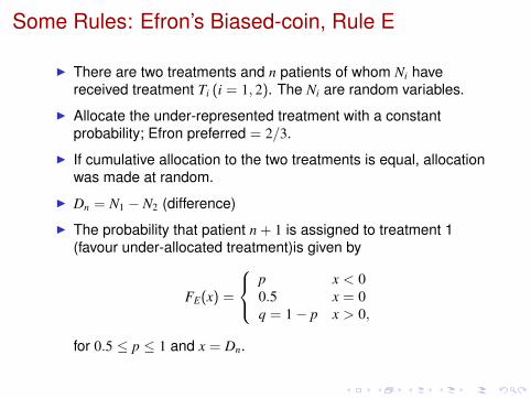
I There are two treatments and n patients of whom Ni havereceived treatment Ti (i = 1, 2). The Ni are random variables.

I Allocate the under-represented treatment with a constantprobability; Efron preferred = 2/3.

I If cumulative allocation to the two treatments is equal, allocationwas made at random.

I Dn = N1 − N2 (difference)

I The probability that patient n + 1 is assigned to treatment 1(favour under-allocated treatment)is given by

FE(x) =

p x < 00.5 x = 0q = 1− p x > 0,

for 0.5 ≤ p ≤ 1 and x = Dn.

Some Rules: Random, R, and Deterministic, D

I Rule R. For p = 0.5 treatment allocation becomes random; nocontrol over balance, but consistent successful guessing of thenext allocation is impossible.

I Rule D. For p = 1 the rule becomes that of sequential designconstruction and |Dn| is either zero, when allocation is at random,or 1, when the under-represented treatment is allocated.

I These two rules are at the extremes of all sensible rules.

I For Rule D the two values of n produce allocations with extremeproperties; random or deterministic.

I The parity of n can have a strong effect on properties

The Adjustable Biased-coin Design: Rule A

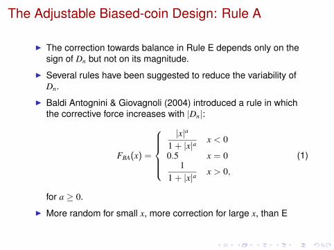
I The correction towards balance in Rule E depends only on thesign of Dn but not on its magnitude.

I Several rules have been suggested to reduce the variability ofDn.

I Baldi Antognini & Giovagnoli (2004) introduced a rule in whichthe corrective force increases with |Dn|:

FBA(x) =

|x|a

1 + |x|ax < 0

0.5 x = 01

1 + |x|ax > 0,

(1)

for a ≥ 0.

I More random for small x, more correction for large x, than E

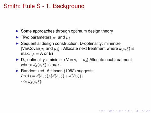
Smith: Rule S - 1. Background

I Some approaches through optimum design theoryI Two parameters µ1 and µ2

I Sequential design construction, D-optimality: minimize|VarCovar(µ1 and µ2)|. Allocate next treatment where d(x, ξ) ismax. (x = A or B)

I DA-optimality : minimize Var(µ1 − µ2) Allocate next treatmentwhere dA(x, ξ) is max.

I Randomized. Atkinson (1982) suggestsPr(A) = d(A, ξ)/{d(A, ξ) + d(B, ξ)}- or dA(x, ξ)

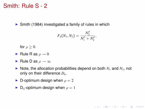
Smith: Rule S - 2

I Smith (1984) investigated a family of rules in which

FS(N1,N2) =Nρ

2

Nρ1 + Nρ

2,

for ρ ≥ 0.

I Rule R as ρ→ 0

I Rule D as ρ→∞I Note, the allocation probabilities depend on both N1 and N2, not

only on their difference Dn.

I D-optimum design when ρ = 2

I DA-optimum design when ρ = 1

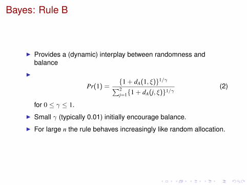
Bayes: Rule B

I Provides a (dynamic) interplay between randomness andbalance

I

Pr(1) ={1 + dA(1, ξ)}1/γ∑2j=1{1 + dA(j, ξ)}1/γ

(2)

for 0 ≤ γ ≤ 1.

I Small γ (typically 0.01) initially encourage balance.

I For large n the rule behaves increasingly like random allocation.

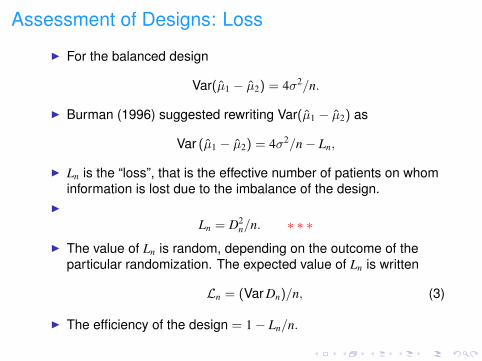
Assessment of Designs: Loss

I For the balanced design

Var(µ1 − µ2) = 4σ2/n.

I Burman (1996) suggested rewriting Var(µ1 − µ2) as

Var (µ1 − µ2) = 4σ2/n− Ln,

I Ln is the “loss”, that is the effective number of patients on whominformation is lost due to the imbalance of the design.

I

Ln = D2n/n. ∗ ∗ ∗

I The value of Ln is random, depending on the outcome of theparticular randomization. The expected value of Ln is written

Ln = (Var Dn)/n, (3)

I The efficiency of the design = 1− Ln/n.

Assessment of Designs: Bias

I Randomization and balance are in conflict.

I Measure randomization by selection bias (Blackwell & Hodges,1957), the ability to guess the next treatment to be allocated.

I The expected bias Bn is estimated from nsim simulations as

Bn = (number of correct guesses of allocation to patient n

−number of incorrect guesses)/nsim.

I Guess that the treatment with the higher allocation probabilitywill be selected.

Analytical Results Rule EI For Rules E and A the distribution of the values of Dn forms a

Markov chain.I Analytical results come from the steady state distribution of Dn.I The value of Bn depends on the distribution of Dn−1, whereas

that of Ln requires the distribution of Dn.I If Dn−1 = 0, allocation to patient n is at random; bias is zero.I For all other values the bias, conditional on the value of Dn−1, is

p− (1− p) = 2p− 1.I The steady-state probabilities that Dn = 0 are given by Efron

(1971) and by Markaryan & Rosenberger (2010). When n is odd,P(D2m 6= 0) = (1− p)/p and

B2m−1 = (2p− 1)(1− p)/p.

I Ln = (Var Dn)/n. Expressions for Var Dn from the steady-statedistribution are given by Markaryan & Rosenberger (2010),hence Ln.

I These values of Ln also depend on whether n is even or odd:

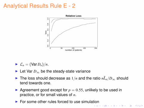
Analytical Results Rule E - 2

0 50 100 150 2000.

00.

20.

40.

60.

81.

0

number of patients

loss

Relative Loss

I Ln = (Var Dn)/n.

I Let Var D∞ be the steady-state variance

I The loss should decrease as 1/n and the ratio nLn/D∞ shouldtend towards one.

I Agreement good except for p = 0.55, unlikely to be used inpractice, or for small values of n.

I For some other rules forced to use simulation

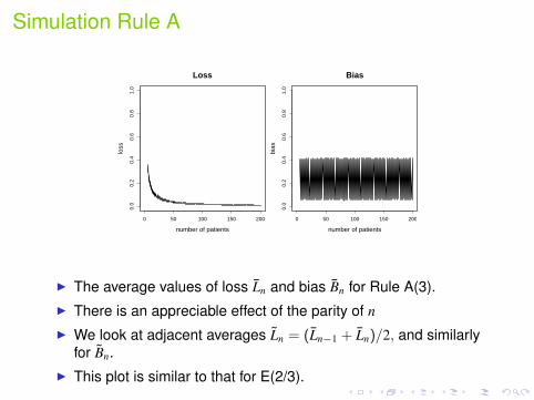
Simulation Rule A

0 50 100 150 200

0.0

0.2

0.4

0.6

0.8

1.0

number of patients

loss

Loss

0 50 100 150 200

0.0

0.2

0.4

0.6

0.8

1.0

number of patients

bias

Bias

I The average values of loss Ln and bias Bn for Rule A(3).I There is an appreciable effect of the parity of n

I We look at adjacent averages Ln = (Ln−1 + Ln)/2, and similarlyfor Bn.

I This plot is similar to that for E(2/3).

Simulations Rules R, E, A and D

0 50 100 150 200

0.0

0.2

0.4

0.6

0.8

1.0

number of patients

loss

R

E

EAD

Loss

0 50 100 150 200

0.0

0.1

0.2

0.3

0.4

0.5

number of patients

bias

R

E

AE

D

Bias

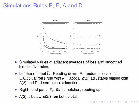
I Simulated values of adjacent averages of loss and smoothedbias for five rules.

I Left-hand panel Ln. Reading down: R, random allocation;E(0.55), Efron’s rule with p = 0.55; E(2/3); adjustable biased coinA(3) and D, deterministic allocation.

I Right-hand panel Bn. Same notation, reading up.

I A(3) is below E(2/3) on both plots!

Simulations Rules B and S

0 50 100 150 200

0.0

0.2

0.4

0.6

0.8

1.0

number of patients

loss

SB

S

B

Loss

0 50 100 150 200

0.0

0.1

0.2

0.3

0.4

0.5

number of patients

bias

S

B

S

B

Bias

I Simulated values of adjacent averages of loss and smoothedbias for four rules.

I Left-hand panel Ln. Reading down: B, Bayes rule with γ = 0.1;B, Bayes rule with γ = 0.01; S, Smith’s rule with ρ = 2 andSmith’s rule with ρ = 5.

I Right-hand panel Bn. Same notation, reading up.I The plots of Ln for Rule S are virtually constantI Those for Rule B increase with n, becoming more like random

allocation

Admissibility

I A good rule has low loss and low bias for all n.

I To compare loss and bias, plot loss against bias as a function ofn, thus combining the two panels in one

I The shape that this curve takes depends upon the individual rule

I There are three general forms of trajectory.

I A good rule will be in the lower left-hand corner of the plot.

I Usually, for a particular n, a rule with lower loss than another willhave higher bias. A rule for which both values are higher is saidto be inadmissible.

Admissibility - 2

0.0 0.1 0.2 0.3 0.4 0.5

0.0

0.2

0.4

0.6

0.8

1.0

bias

loss

R

E

A

SD

B

0.20 0.22 0.24 0.26 0.28 0.30

0.0

0.1

0.2

0.3

0.4

bias

loss EA

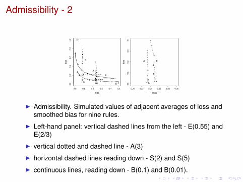
I Admissibility. Simulated values of adjacent averages of loss andsmoothed bias for nine rules.

I Left-hand panel: vertical dashed lines from the left - E(0.55) andE(2/3)

I vertical dotted and dashed line - A(3)

I horizontal dashed lines reading down - S(2) and S(5)

I continuous lines, reading down - B(0.1) and B(0.01).

Admissibility - 3

0.0 0.1 0.2 0.3 0.4 0.5

0.0

0.2

0.4

0.6

0.8

1.0

bias

loss

R

E

A

SD

B

0.20 0.22 0.24 0.26 0.28 0.30

0.0

0.1

0.2

0.3

0.4

bias

loss EA

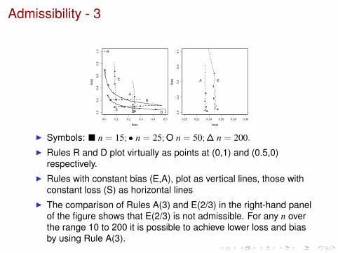
I Symbols: � n = 15; • n = 25; O n = 50; ∆ n = 200.I Rules R and D plot virtually as points at (0,1) and (0.5,0)

respectively.I Rules with constant bias (E,A), plot as vertical lines, those with

constant loss (S) as horizontal linesI The comparison of Rules A(3) and E(2/3) in the right-hand panel

of the figure shows that E(2/3) is not admissible. For any n overthe range 10 to 200 it is possible to achieve lower loss and biasby using Rule A(3).

Conclusion

I Bayes (Rule B) forces balance when n is small, becoming morerandom as n increases.

I The effect on design efficiency is relatively small for large n (herelose information on one patient).

I The allocation becomes increasingly random as n ↑ ∞ and biasgoes to zero.

Some References

Atkinson, A. C. (1982). Optimum biased coin designs for sequential clinical trials withprognostic factors. Biometrika, 69, 61–67.

Baldi Antognini, A. & Giovagnoli, A. (2004). A new ‘biased coin design’ for thesequential allocation of two treatments. Applied Statistics, 53, 651–664.

Blackwell, D. & Hodges, J. L. (1957). Design for the control of selection bias. Annals ofMathematical Statistics, 28, 449–460.

Burman, C.-F. (1996). On Sequential Treatment Allocations in Clinical Trials.Department of Mathematics, Goteborg.

Efron, B. (1971). Forcing a sequential experiment to be balanced. Biometrika, 58,403–417.

Markaryan, T. & Rosenberger, W. F. (2010). Exact properties of Efron’s biased coinrandomization procedure. Annals of Statistics, 38, 1546–1567.

Smith, R. L. (1984). Sequential treatment allocation using biased coin designs. Journalof the Royal Statistical Society, Series B, 46, 519—543.