Randomized Algorithms and Motif Finding - UCSD...
65
www.bioalgorithms.info An Introduction to Bioinformatics Algorithms Randomized Algorithms and Motif Finding
Transcript of Randomized Algorithms and Motif Finding - UCSD...

www.bioalgorithms.infoAn Introduction to Bioinformatics Algorithms
Randomized Algorithmsand Motif Finding
An Introduction to Bioinformatics Algorithms www.bioalgorithms.info
Outline• Randomized QuickSort• Randomized Algorithms• Greedy Profile Motif Search• Gibbs Sampler• Random Projections
An Introduction to Bioinformatics Algorithms www.bioalgorithms.info
Randomized Algorithms• Randomized algorithms make random rather
than deterministic decisions.• The main advantage is that no input can
reliably produce worst-case results because the algorithm runs differently each time.
• These algorithms are commonly used in situations where no exact and fast algorithm is known.
An Introduction to Bioinformatics Algorithms www.bioalgorithms.info
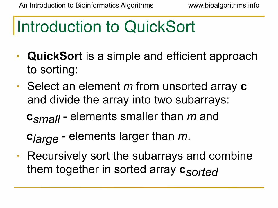
Introduction to QuickSort• QuickSort is a simple and efficient approach
to sorting:• Select an element m from unsorted array c
and divide the array into two subarrays:
csmall - elements smaller than m and
clarge - elements larger than m.
• Recursively sort the subarrays and combine them together in sorted array csorted
An Introduction to Bioinformatics Algorithms www.bioalgorithms.info
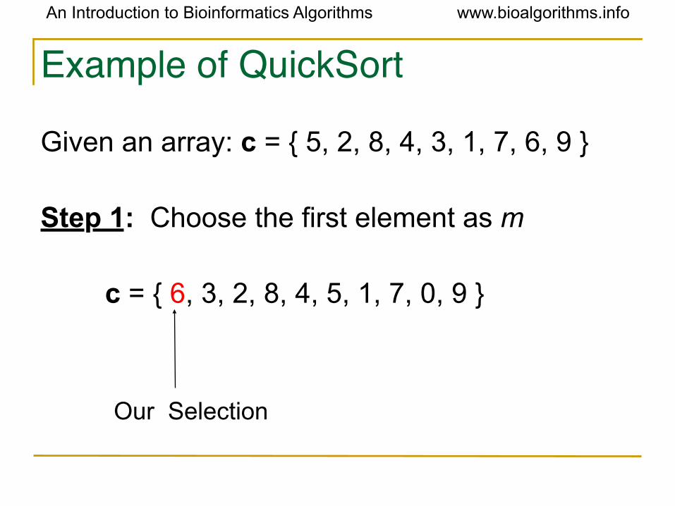
Example of QuickSort
Given an array: c = { 5, 2, 8, 4, 3, 1, 7, 6, 9 }
Step 1: Choose the first element as m
c = { 6, 3, 2, 8, 4, 5, 1, 7, 0, 9 }
Our Selection
An Introduction to Bioinformatics Algorithms www.bioalgorithms.info
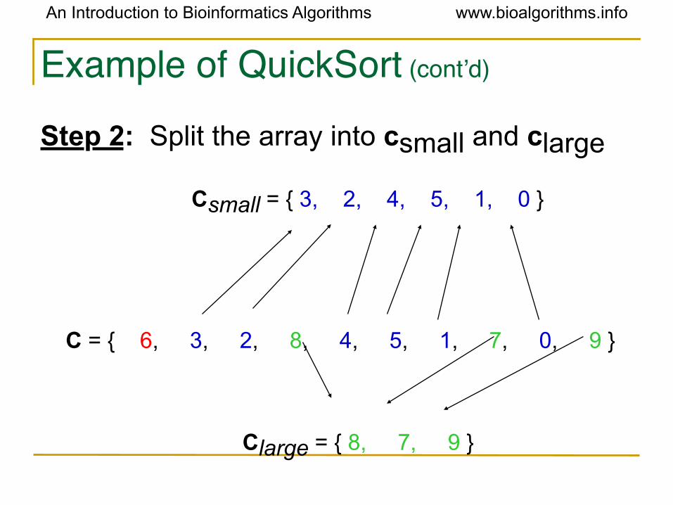
Example of QuickSort (cont’d)
Step 2: Split the array into csmall and clarge
Csmall = { 3, 2, 4, 5, 1, 0 }
C = { 6, 3, 2, 8, 4, 5, 1, 7, 0, 9 }
Clarge = { 8, 7, 9 }
An Introduction to Bioinformatics Algorithms www.bioalgorithms.info
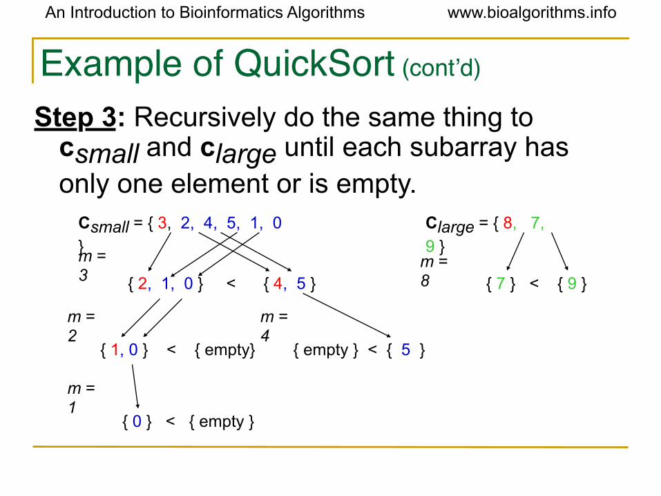
Example of QuickSort (cont’d)
Step 3: Recursively do the same thing to csmall and clarge until each subarray has only one element or is empty.
Csmall = { 3, 2, 4, 5, 1, 0
}
Clarge = { 8, 7,
9 }m = 3
m = 8{ 2, 1, 0 } < { 4, 5 } { 7 } < { 9 }
m = 2
{ 1, 0 } < { empty} { empty } < { 5 }
m = 4
m = 1
{ 0 } < { empty }
An Introduction to Bioinformatics Algorithms www.bioalgorithms.info
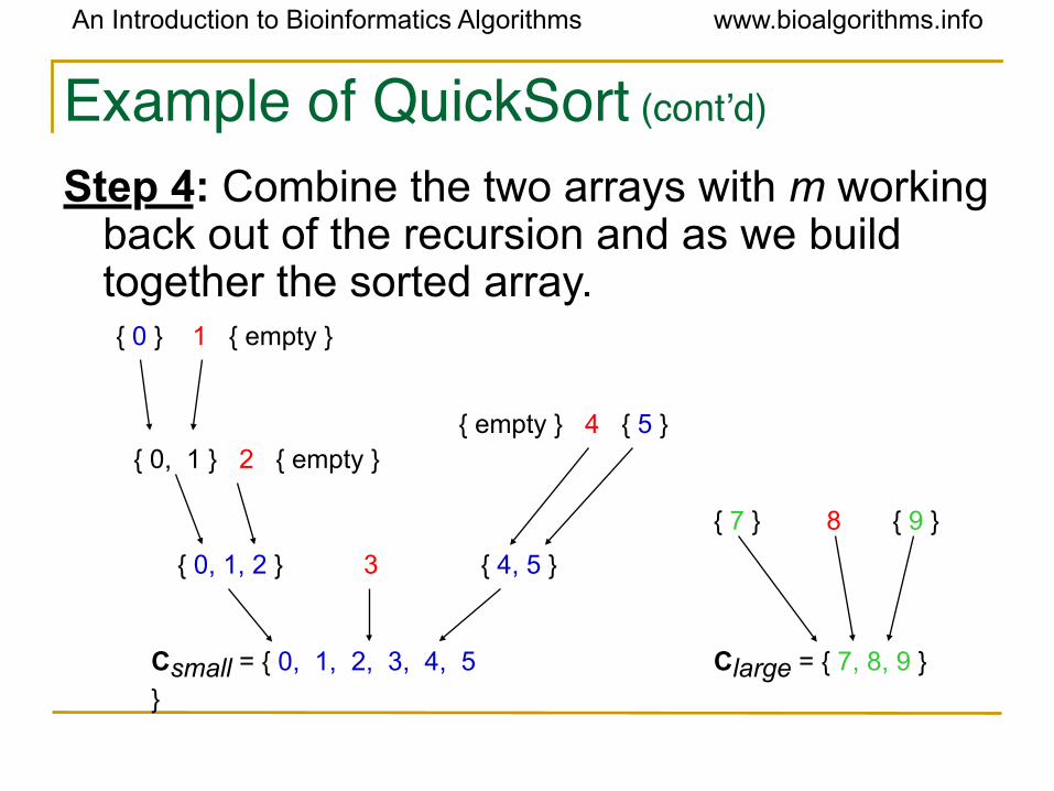
Example of QuickSort (cont’d)
Step 4: Combine the two arrays with m working back out of the recursion and as we build together the sorted array.
Csmall = { 0, 1, 2, 3, 4, 5
}
Clarge = { 7, 8, 9 }
{ 0, 1, 2 } 3 { 4, 5 }
{ 7 } 8 { 9 }
{ 0, 1 } 2 { empty }{ empty } 4 { 5 }
{ 0 } 1 { empty }
An Introduction to Bioinformatics Algorithms www.bioalgorithms.info
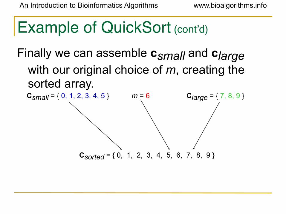
Example of QuickSort (cont’d)
Finally we can assemble csmall and clarge
with our original choice of m, creating the sorted array.Csmall = { 0, 1, 2, 3, 4, 5 } Clarge = { 7, 8, 9 }m = 6
Csorted = { 0, 1, 2, 3, 4, 5, 6, 7, 8, 9 }
An Introduction to Bioinformatics Algorithms www.bioalgorithms.info
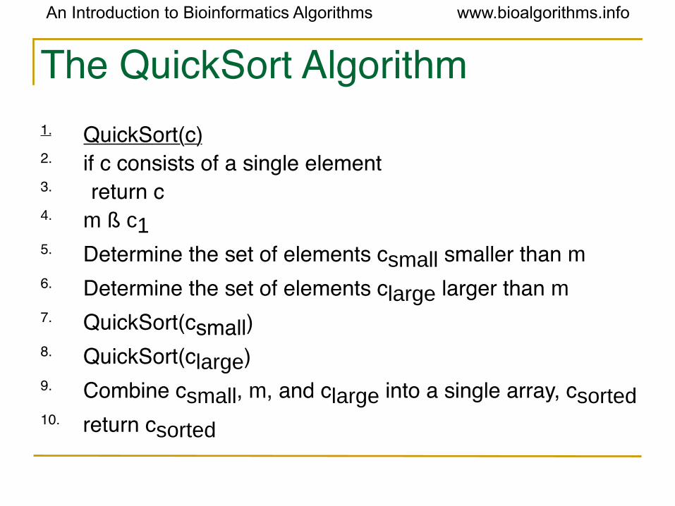
The QuickSort Algorithm1. QuickSort(c)2. if c consists of a single element3. return c4. m ß c15. Determine the set of elements csmall smaller than m6. Determine the set of elements clarge larger than m7. QuickSort(csmall)8. QuickSort(clarge)9. Combine csmall, m, and clarge into a single array, csorted10. return csorted
An Introduction to Bioinformatics Algorithms www.bioalgorithms.info
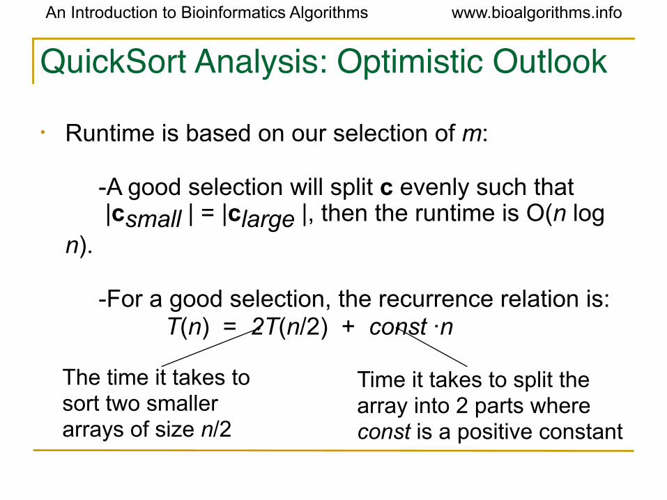
QuickSort Analysis: Optimistic Outlook
• Runtime is based on our selection of m:
-A good selection will split c evenly such that |csmall | = |clarge |, then the runtime is O(n log
n).
-For a good selection, the recurrence relation is:T(n) = 2T(n/2) + const ·n
Time it takes to split the array into 2 parts where const is a positive constant
The time it takes to sort two smaller arrays of size n/2
An Introduction to Bioinformatics Algorithms www.bioalgorithms.info
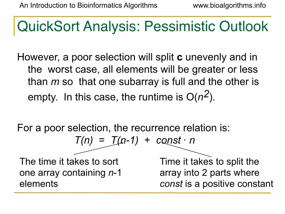
QuickSort Analysis: Pessimistic Outlook
However, a poor selection will split c unevenly and in the worst case, all elements will be greater or less than m so that one subarray is full and the other is
empty. In this case, the runtime is O(n2).
For a poor selection, the recurrence relation is:T(n) = T(n-1) + const · n
The time it takes to sort one array containing n-1 elements
Time it takes to split the array into 2 parts where const is a positive constant
An Introduction to Bioinformatics Algorithms www.bioalgorithms.info
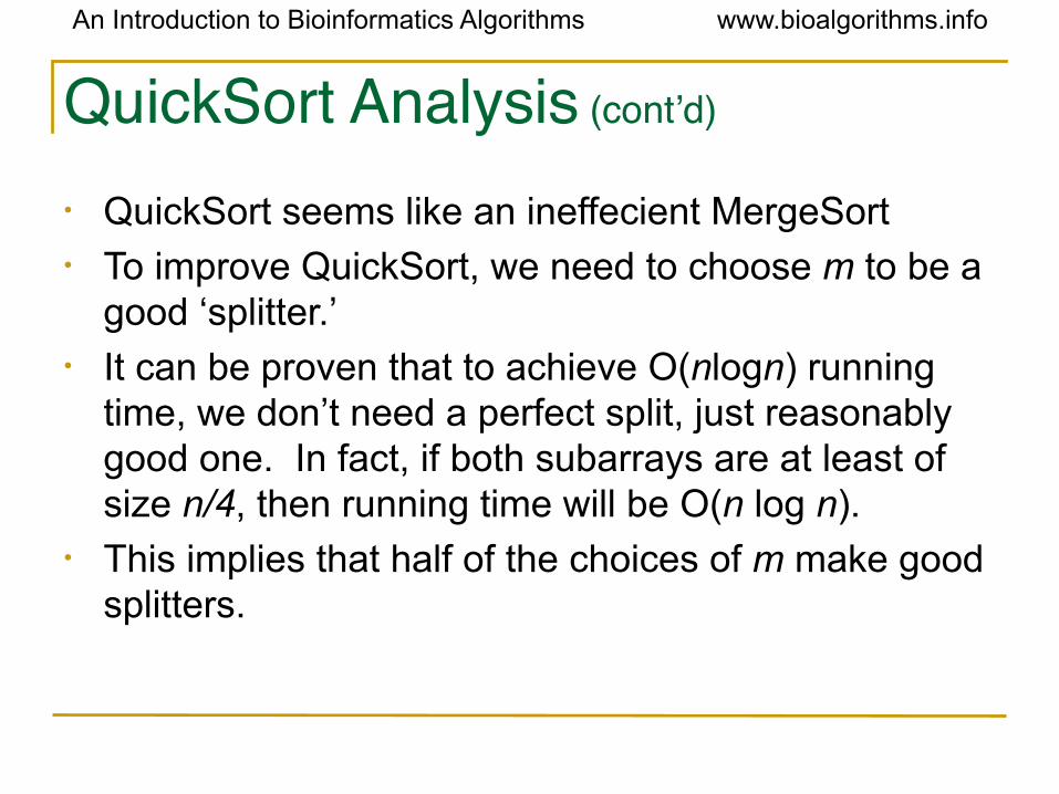
QuickSort Analysis (cont’d)
• QuickSort seems like an ineffecient MergeSort• To improve QuickSort, we need to choose m to be a
good ‘splitter.’• It can be proven that to achieve O(nlogn) running
time, we don’t need a perfect split, just reasonably good one. In fact, if both subarrays are at least of size n/4, then running time will be O(n log n).
• This implies that half of the choices of m make good splitters.
An Introduction to Bioinformatics Algorithms www.bioalgorithms.info
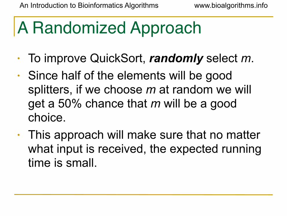
A Randomized Approach• To improve QuickSort, randomly select m.• Since half of the elements will be good
splitters, if we choose m at random we will get a 50% chance that m will be a good choice.
• This approach will make sure that no matter what input is received, the expected running time is small.
An Introduction to Bioinformatics Algorithms www.bioalgorithms.info
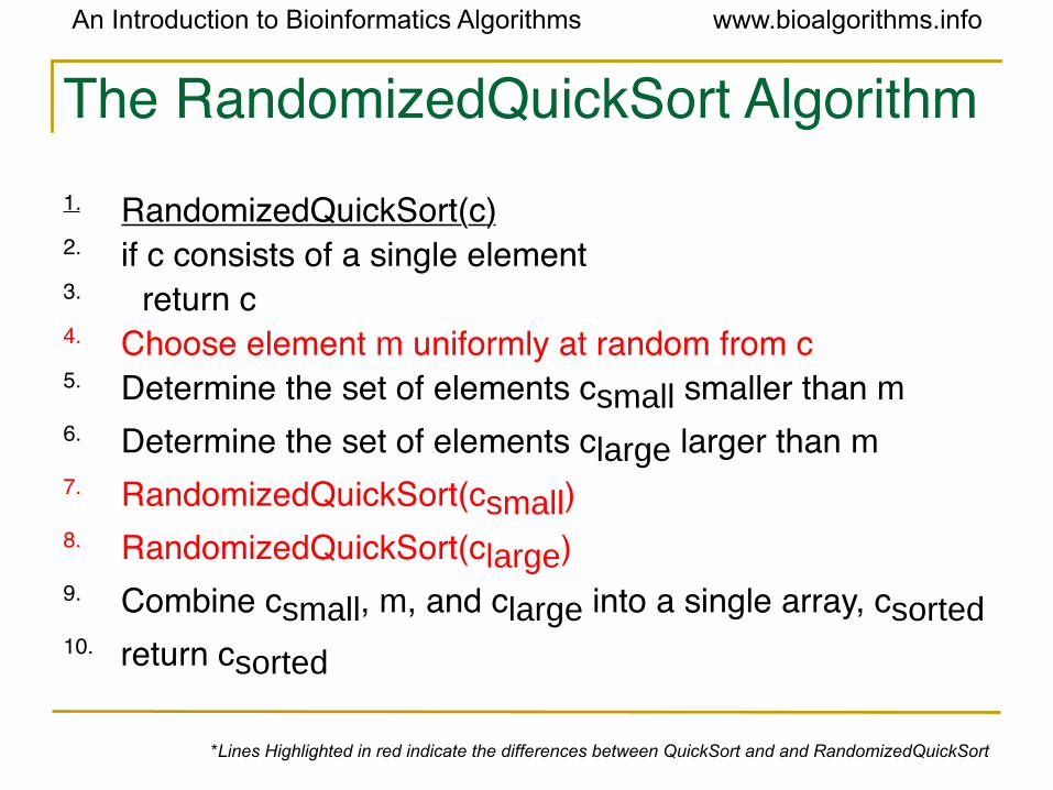
The RandomizedQuickSort Algorithm1. RandomizedQuickSort(c)2. if c consists of a single element3. return c4. Choose element m uniformly at random from c5. Determine the set of elements csmall smaller than m6. Determine the set of elements clarge larger than m7. RandomizedQuickSort(csmall)8. RandomizedQuickSort(clarge)9. Combine csmall, m, and clarge into a single array, csorted10. return csorted
*Lines Highlighted in red indicate the differences between QuickSort and and RandomizedQuickSort
An Introduction to Bioinformatics Algorithms www.bioalgorithms.info
RandomizedQuickSort Analysis• Worst case runtime: O(m2)• Expected runtime: O(m log m).• Expected runtime is a good measure of the
performance of randomized algorithms, often more informative than worst case runtimes.
• RandomizedQuickSort will always return the correct answer, which offers a way to classify Randomized Algorithms.
An Introduction to Bioinformatics Algorithms www.bioalgorithms.info
Two Types of Randomized Algorithms
• Las Vegas Algorithms – always produce the correct solution (ie. RandomizedQuickSort)
• Monte Carlo Algorithms – do not always return the correct solution.
• Las Vegas Algorithms are always preferred, but they are often hard to come by.
An Introduction to Bioinformatics Algorithms www.bioalgorithms.info
The Motif Finding ProblemMotif Finding Problem: Given a list of t
sequences each of length n, find the “best” pattern of length l that appears in each of the t sequences.
An Introduction to Bioinformatics Algorithms www.bioalgorithms.info
A New Motif Finding Approach• Motif Finding Problem: Given a list of t
sequences each of length n, find the “best” pattern of length l that appears in each of the t sequences.
• Previously: we solved the Motif Finding Problem using a Branch and Bound or a Greedy technique.
• Now: randomly select possible locations and find a way to greedily change those locations until we have converged to the hidden motif.
An Introduction to Bioinformatics Algorithms www.bioalgorithms.info
Profiles Revisited• Let s=(s1,...,st) be the set of starting
positions for l-mers in our t sequences. • The substrings corresponding to these
starting positions will form: - t x l alignment matrix and - 4 x l profile matrix* P.
*We make a special note that the profile matrix will be defined in terms of the frequency of letters, and not as the count of letters.
An Introduction to Bioinformatics Algorithms www.bioalgorithms.info
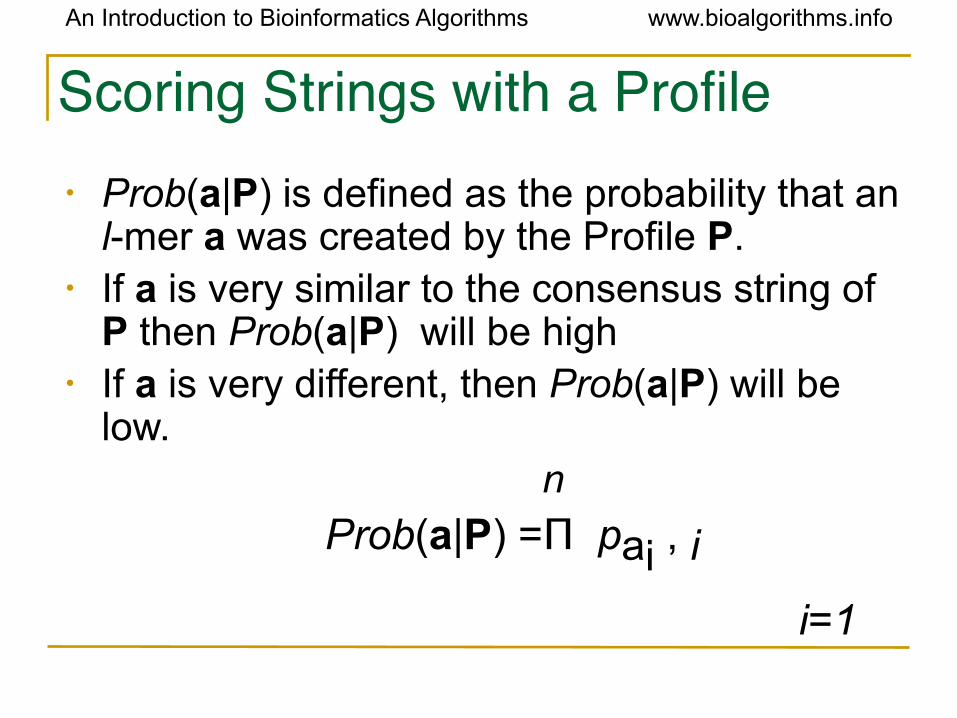
• Prob(a|P) is defined as the probability that an l-mer a was created by the Profile P.
• If a is very similar to the consensus string of P then Prob(a|P) will be high
• If a is very different, then Prob(a|P) will be low.
n
Prob(a|P) =Π pai , i
i=1
Scoring Strings with a Profile
An Introduction to Bioinformatics Algorithms www.bioalgorithms.info
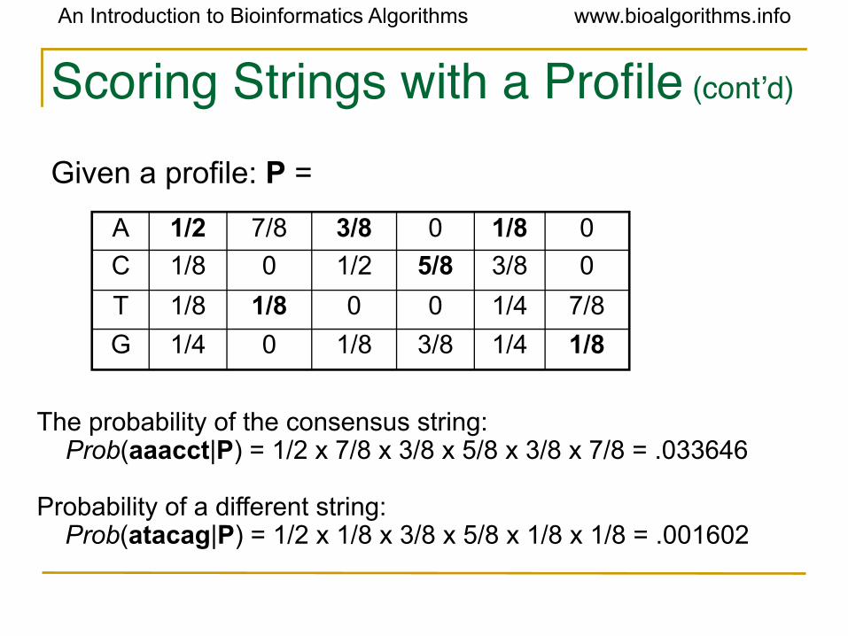
Scoring Strings with a Profile (cont’d)
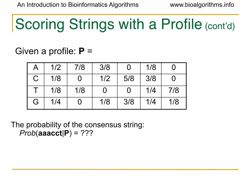
Given a profile: P =
A 1/2 7/8 3/8 0 1/8 0
C 1/8 0 1/2 5/8 3/8 0
T 1/8 1/8 0 0 1/4 7/8
G 1/4 0 1/8 3/8 1/4 1/8
Prob(aaacct|P) = ??? The probability of the consensus string:
An Introduction to Bioinformatics Algorithms www.bioalgorithms.info
Scoring Strings with a Profile (cont’d)
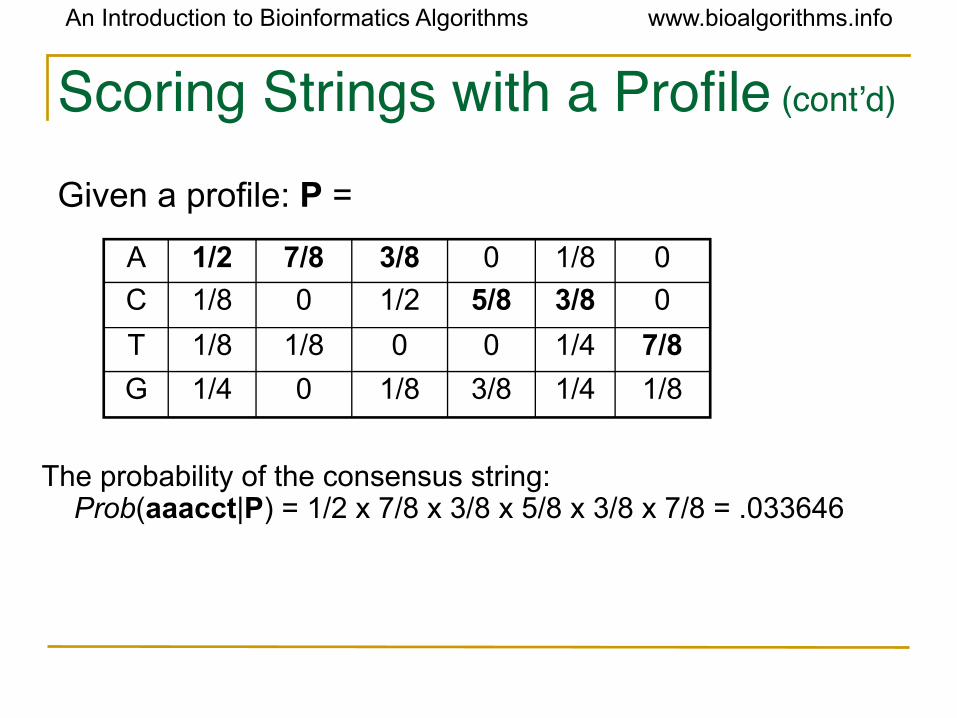
Given a profile: P =
A 1/2 7/8 3/8 0 1/8 0
C 1/8 0 1/2 5/8 3/8 0
T 1/8 1/8 0 0 1/4 7/8
G 1/4 0 1/8 3/8 1/4 1/8
Prob(aaacct|P) = 1/2 x 7/8 x 3/8 x 5/8 x 3/8 x 7/8 = .033646The probability of the consensus string:
An Introduction to Bioinformatics Algorithms www.bioalgorithms.info
Scoring Strings with a Profile (cont’d)
Given a profile: P =
A 1/2 7/8 3/8 0 1/8 0
C 1/8 0 1/2 5/8 3/8 0
T 1/8 1/8 0 0 1/4 7/8
G 1/4 0 1/8 3/8 1/4 1/8
Prob(atacag|P) = 1/2 x 1/8 x 3/8 x 5/8 x 1/8 x 1/8 = .001602
Prob(aaacct|P) = 1/2 x 7/8 x 3/8 x 5/8 x 3/8 x 7/8 = .033646The probability of the consensus string:
Probability of a different string:
An Introduction to Bioinformatics Algorithms www.bioalgorithms.info
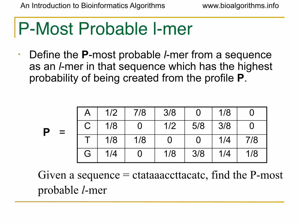
P-Most Probable l-mer• Define the P-most probable l-mer from a sequence
as an l-mer in that sequence which has the highest probability of being created from the profile P.
A 1/2 7/8 3/8 0 1/8 0
C 1/8 0 1/2 5/8 3/8 0
T 1/8 1/8 0 0 1/4 7/8
G 1/4 0 1/8 3/8 1/4 1/8
P =
Given a sequence = ctataaaccttacatc, find the P-most probable l-mer
An Introduction to Bioinformatics Algorithms www.bioalgorithms.info
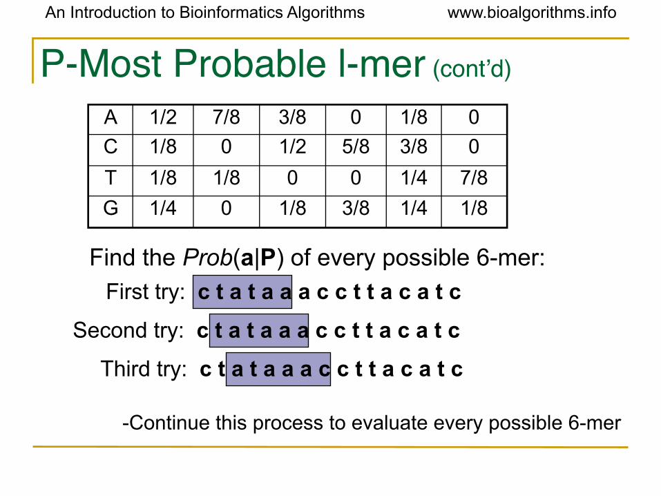
Third try: c t a t a a a c c t t a c a t c
Second try: c t a t a a a c c t t a c a t c
First try: c t a t a a a c c t t a c a t c
P-Most Probable l-mer (cont’d)
A 1/2 7/8 3/8 0 1/8 0
C 1/8 0 1/2 5/8 3/8 0
T 1/8 1/8 0 0 1/4 7/8
G 1/4 0 1/8 3/8 1/4 1/8
Find the Prob(a|P) of every possible 6-mer:
-Continue this process to evaluate every possible 6-mer
An Introduction to Bioinformatics Algorithms www.bioalgorithms.info
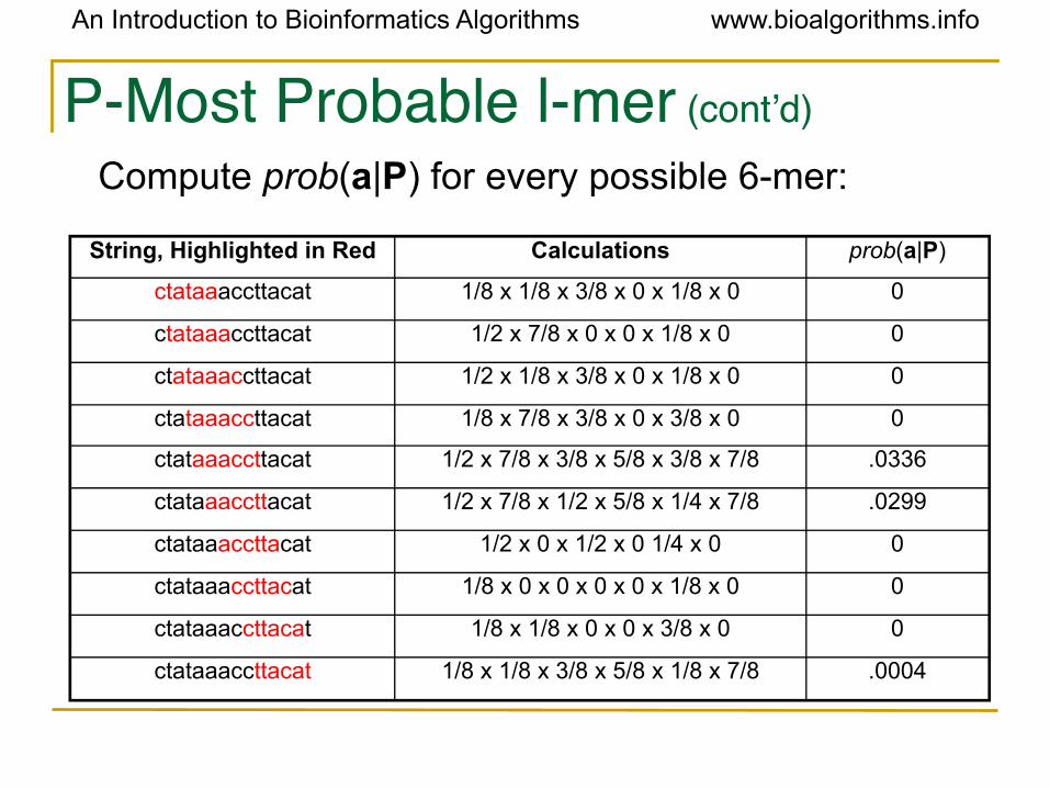
P-Most Probable l-mer (cont’d)
String, Highlighted in Red Calculations prob(a|P)
ctataaaccttacat 1/8 x 1/8 x 3/8 x 0 x 1/8 x 0 0
ctataaaccttacat 1/2 x 7/8 x 0 x 0 x 1/8 x 0 0
ctataaaccttacat 1/2 x 1/8 x 3/8 x 0 x 1/8 x 0 0
ctataaaccttacat 1/8 x 7/8 x 3/8 x 0 x 3/8 x 0 0
ctataaaccttacat 1/2 x 7/8 x 3/8 x 5/8 x 3/8 x 7/8 .0336
ctataaaccttacat 1/2 x 7/8 x 1/2 x 5/8 x 1/4 x 7/8 .0299
ctataaaccttacat 1/2 x 0 x 1/2 x 0 1/4 x 0 0
ctataaaccttacat 1/8 x 0 x 0 x 0 x 0 x 1/8 x 0 0
ctataaaccttacat 1/8 x 1/8 x 0 x 0 x 3/8 x 0 0
ctataaaccttacat 1/8 x 1/8 x 3/8 x 5/8 x 1/8 x 7/8 .0004
Compute prob(a|P) for every possible 6-mer:
An Introduction to Bioinformatics Algorithms www.bioalgorithms.info
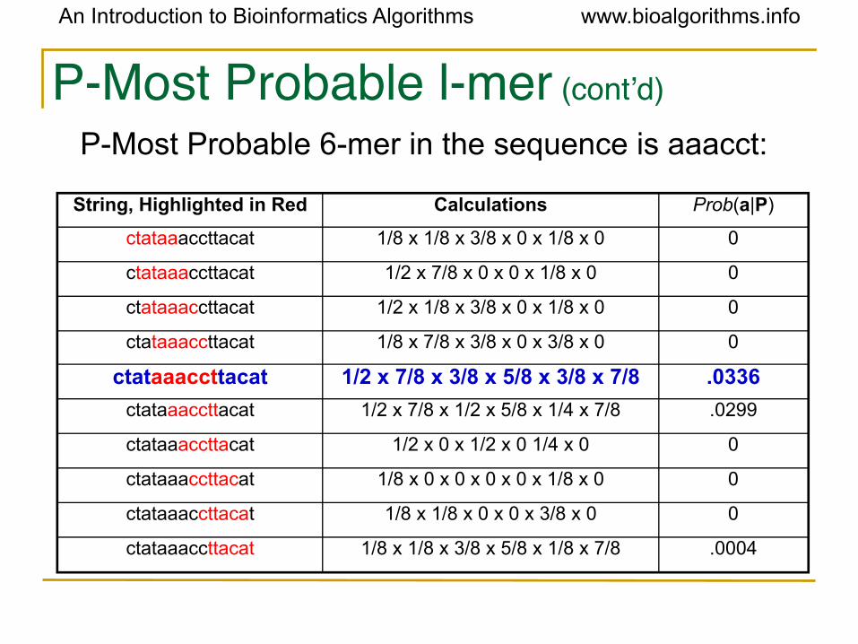
P-Most Probable l-mer (cont’d)
String, Highlighted in Red Calculations Prob(a|P)
ctataaaccttacat 1/8 x 1/8 x 3/8 x 0 x 1/8 x 0 0
ctataaaccttacat 1/2 x 7/8 x 0 x 0 x 1/8 x 0 0
ctataaaccttacat 1/2 x 1/8 x 3/8 x 0 x 1/8 x 0 0
ctataaaccttacat 1/8 x 7/8 x 3/8 x 0 x 3/8 x 0 0
ctataaaccttacat 1/2 x 7/8 x 3/8 x 5/8 x 3/8 x 7/8 .0336
ctataaaccttacat 1/2 x 7/8 x 1/2 x 5/8 x 1/4 x 7/8 .0299
ctataaaccttacat 1/2 x 0 x 1/2 x 0 1/4 x 0 0
ctataaaccttacat 1/8 x 0 x 0 x 0 x 0 x 1/8 x 0 0
ctataaaccttacat 1/8 x 1/8 x 0 x 0 x 3/8 x 0 0
ctataaaccttacat 1/8 x 1/8 x 3/8 x 5/8 x 1/8 x 7/8 .0004
P-Most Probable 6-mer in the sequence is aaacct:
An Introduction to Bioinformatics Algorithms www.bioalgorithms.info
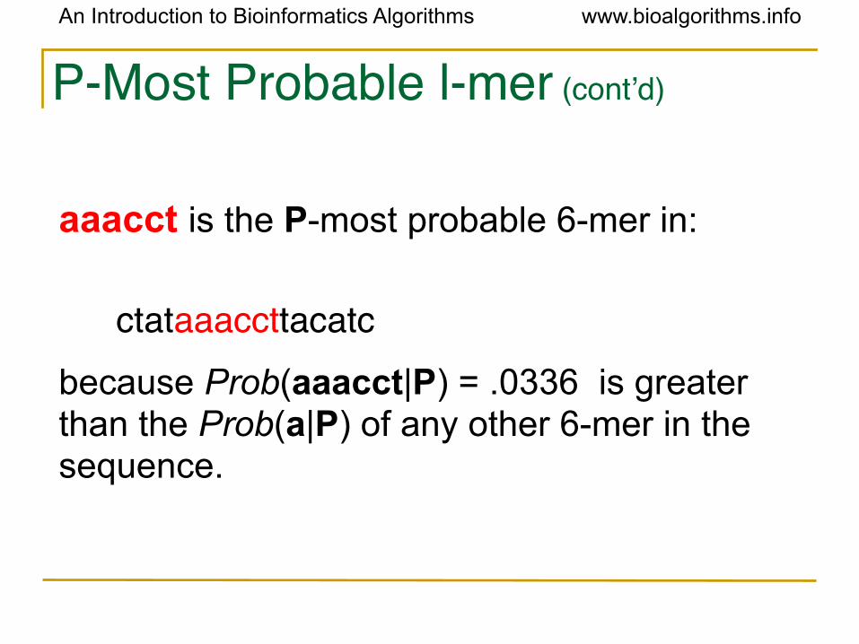
P-Most Probable l-mer (cont’d)
ctataaaccttacatcbecause Prob(aaacct|P) = .0336 is greater than the Prob(a|P) of any other 6-mer in the sequence.
aaacct is the P-most probable 6-mer in:
An Introduction to Bioinformatics Algorithms www.bioalgorithms.info
Dealing with Zeroes
• In our toy example prob(a|P)=0 in many cases. In practice, there will be enough sequences so that the number of elements in the profile with a frequency of zero is small.
• To avoid many entries with prob(a|P)=0, there exist techniques to equate zero to a very small number so that one zero does not make the entire probability of a string zero (we will not address these techniques here).
An Introduction to Bioinformatics Algorithms www.bioalgorithms.info
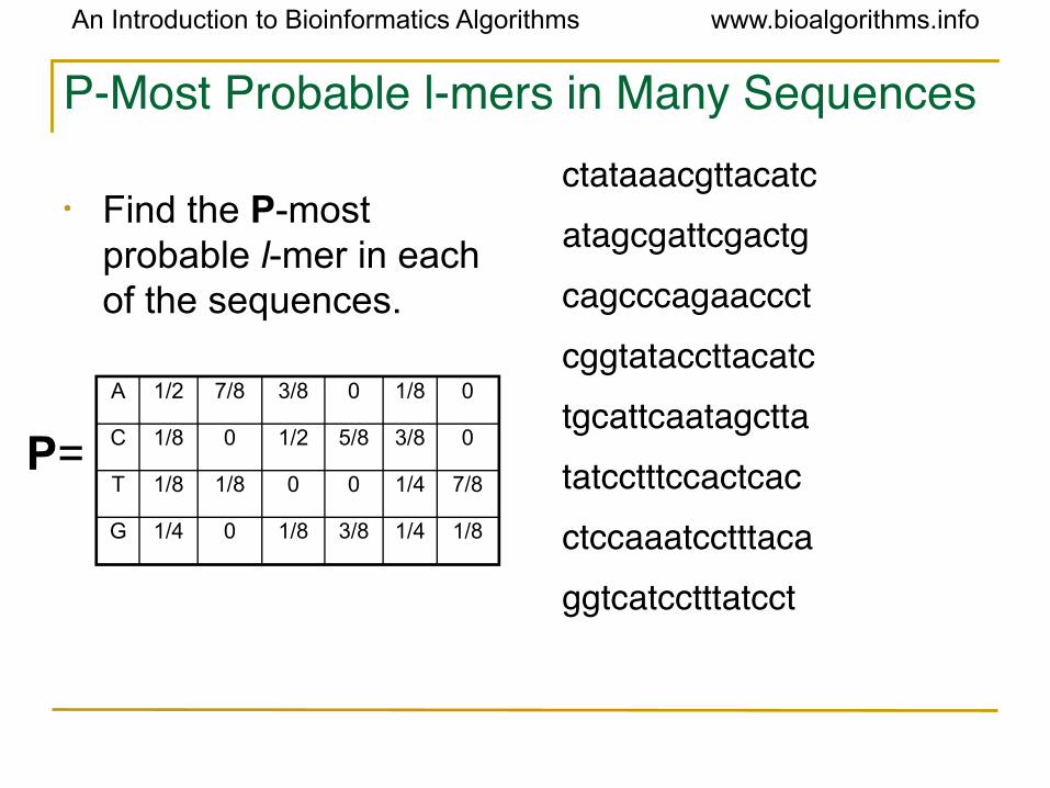
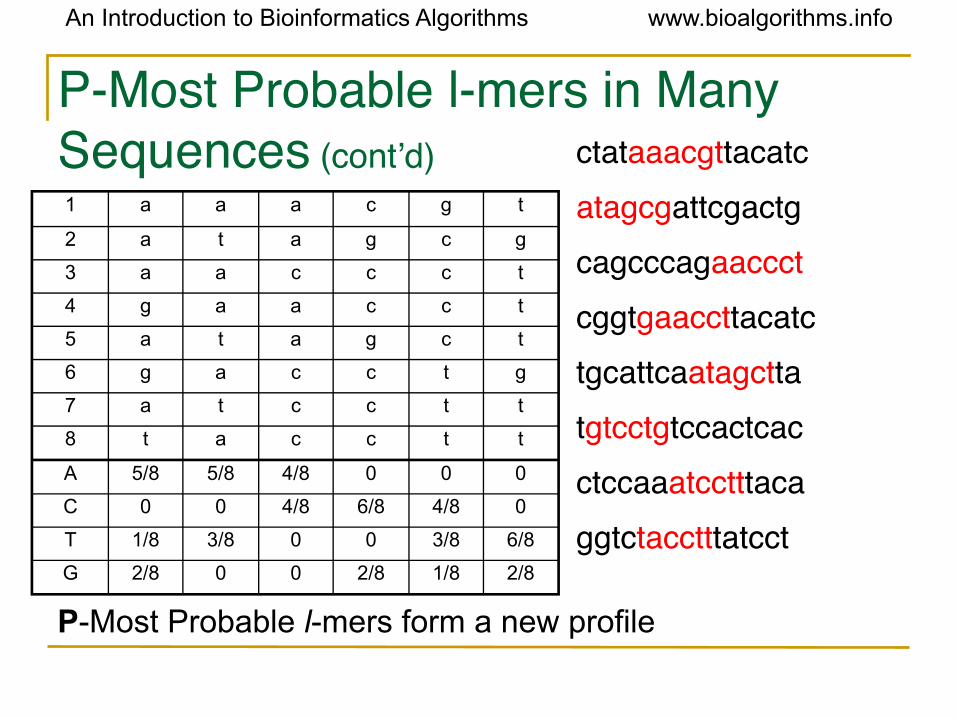
P-Most Probable l-mers in Many Sequences
• Find the P-most probable l-mer in each of the sequences.
ctataaacgttacatcatagcgattcgactgcagcccagaaccctcggtataccttacatctgcattcaatagcttatatcctttccactcacctccaaatcctttacaggtcatcctttatcct
A 1/2 7/8 3/8 0 1/8 0
C 1/8 0 1/2 5/8 3/8 0
T 1/8 1/8 0 0 1/4 7/8
G 1/4 0 1/8 3/8 1/4 1/8
P=
An Introduction to Bioinformatics Algorithms www.bioalgorithms.info
P-Most Probable l-mers in Many Sequences (cont’d) ctataaacgttacatc
atagcgattcgactgcagcccagaaccctcggtgaaccttacatctgcattcaatagcttatgtcctgtccactcacctccaaatcctttacaggtctacctttatcct
P-Most Probable l-mers form a new profile
1 a a a c g t
2 a t a g c g
3 a a c c c t
4 g a a c c t
5 a t a g c t
6 g a c c t g
7 a t c c t t
8 t a c c t t
A 5/8 5/8 4/8 0 0 0
C 0 0 4/8 6/8 4/8 0
T 1/8 3/8 0 0 3/8 6/8
G 2/8 0 0 2/8 1/8 2/8
An Introduction to Bioinformatics Algorithms www.bioalgorithms.info
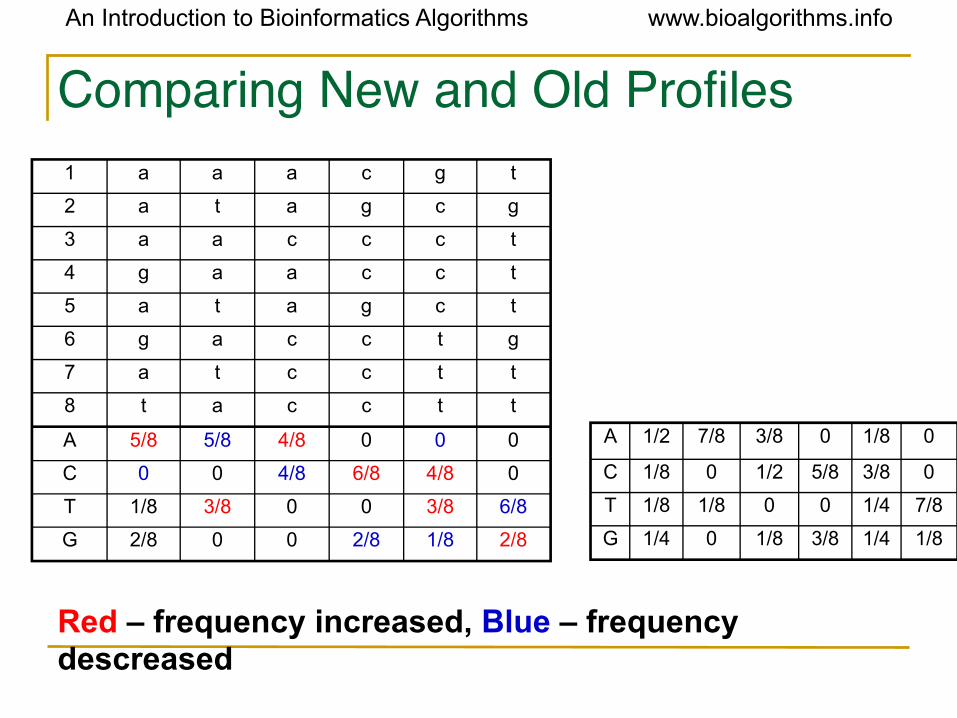
Comparing New and Old Profiles
Red – frequency increased, Blue – frequency descreased
1 a a a c g t
2 a t a g c g
3 a a c c c t
4 g a a c c t
5 a t a g c t
6 g a c c t g
7 a t c c t t
8 t a c c t t
A 5/8 5/8 4/8 0 0 0
C 0 0 4/8 6/8 4/8 0
T 1/8 3/8 0 0 3/8 6/8
G 2/8 0 0 2/8 1/8 2/8
A 1/2 7/8 3/8 0 1/8 0
C 1/8 0 1/2 5/8 3/8 0
T 1/8 1/8 0 0 1/4 7/8
G 1/4 0 1/8 3/8 1/4 1/8
An Introduction to Bioinformatics Algorithms www.bioalgorithms.info
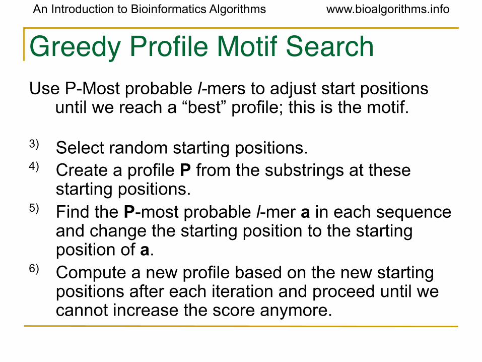
Greedy Profile Motif SearchUse P-Most probable l-mers to adjust start positions
until we reach a “best” profile; this is the motif.
3) Select random starting positions.4) Create a profile P from the substrings at these
starting positions.5) Find the P-most probable l-mer a in each sequence
and change the starting position to the starting position of a.
6) Compute a new profile based on the new starting positions after each iteration and proceed until we cannot increase the score anymore.
An Introduction to Bioinformatics Algorithms www.bioalgorithms.info
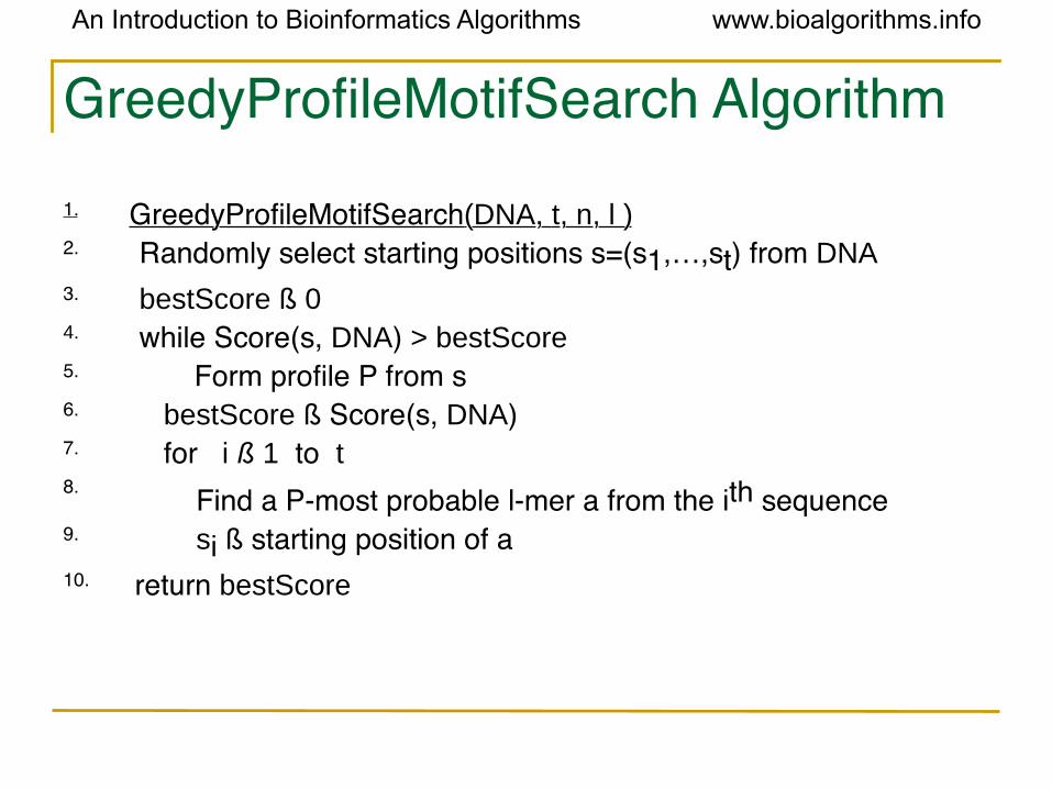
GreedyProfileMotifSearch Algorithm1. GreedyProfileMotifSearch(DNA, t, n, l )2. Randomly select starting positions s=(s1,…,st) from DNA3. bestScore ß 04. while Score(s, DNA) > bestScore5. Form profile P from s6. bestScore ß Score(s, DNA)7. for i ß 1 to t8. Find a P-most probable l-mer a from the ith sequence9. si ß starting position of a10. return bestScore
An Introduction to Bioinformatics Algorithms www.bioalgorithms.info
GreedyProfileMotifSearch Analysis
• Since we choose starting positions randomly, there is little chance that our guess will be close to an optimal motif, meaning it will take a very long time to find the optimal motif.
• It is unlikely that the random starting positions will lead us to the correct solution at all.
• In practice, this algorithm is run many times with the hope that random starting positions will be close to the optimum solution simply by chance.
An Introduction to Bioinformatics Algorithms www.bioalgorithms.info
Gibbs Sampling• GreedyProfileMotifSearch is probably not the
best way to find motifs.• However, we can improve the algorithm by
introducing Gibbs Sampling, an iterative procedure that discards one l-mer after each iteration and replaces it with a new one.
• Gibbs Sampling proceeds more slowly and chooses new l-mers at random increasing the odds that it will converge to the correct solution.
An Introduction to Bioinformatics Algorithms www.bioalgorithms.info
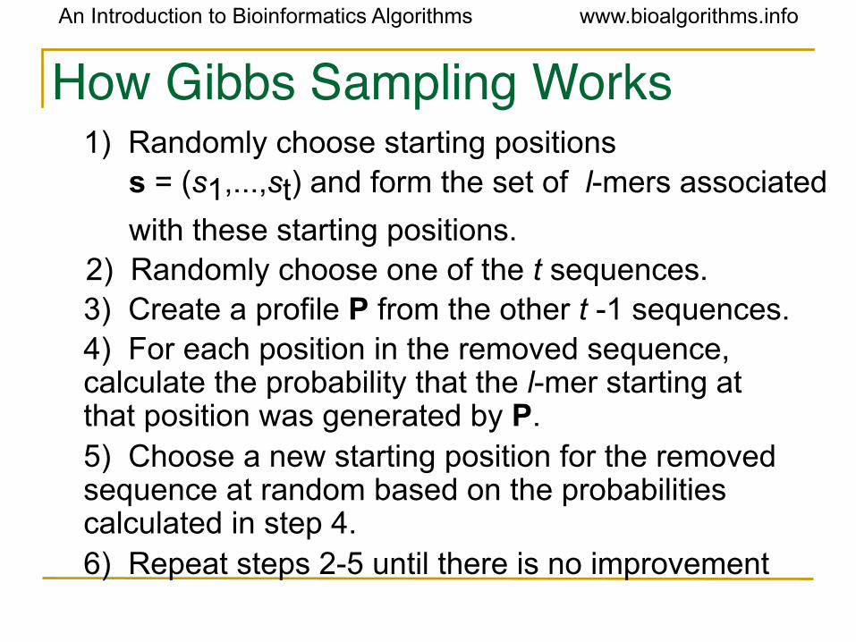
How Gibbs Sampling Works1) Randomly choose starting positions
s = (s1,...,st) and form the set of l-mers associated
with these starting positions. 2) Randomly choose one of the t sequences.
3) Create a profile P from the other t -1 sequences.4) For each position in the removed sequence, calculate the probability that the l-mer starting at that position was generated by P.5) Choose a new starting position for the removed sequence at random based on the probabilities calculated in step 4.6) Repeat steps 2-5 until there is no improvement
An Introduction to Bioinformatics Algorithms www.bioalgorithms.info
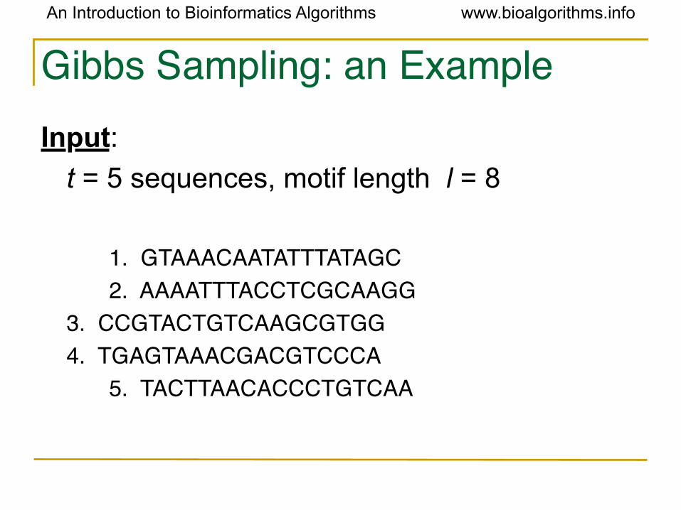
Gibbs Sampling: an ExampleInput:
t = 5 sequences, motif length l = 8
1. GTAAACAATATTTATAGC2. AAAATTTACCTCGCAAGG
3. CCGTACTGTCAAGCGTGG 4. TGAGTAAACGACGTCCCA
5. TACTTAACACCCTGTCAA
An Introduction to Bioinformatics Algorithms www.bioalgorithms.info
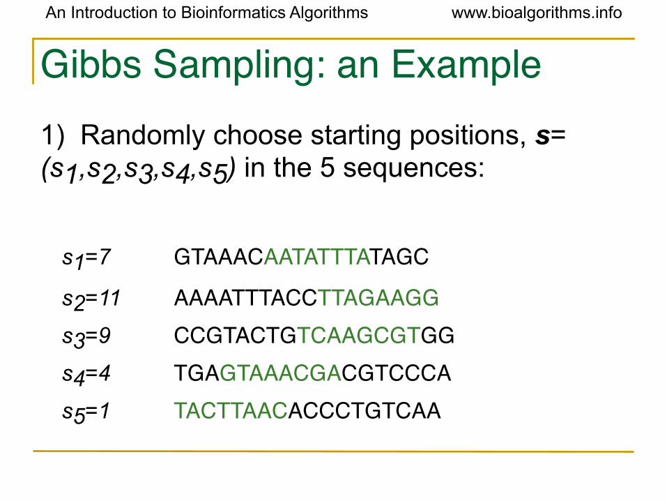
Gibbs Sampling: an Example1) Randomly choose starting positions, s=(s1,s2,s3,s4,s5) in the 5 sequences:
s1=7 GTAAACAATATTTATAGC
s2=11 AAAATTTACCTTAGAAGGs3=9 CCGTACTGTCAAGCGTGGs4=4 TGAGTAAACGACGTCCCAs5=1 TACTTAACACCCTGTCAA
An Introduction to Bioinformatics Algorithms www.bioalgorithms.info
Gibbs Sampling: an Example
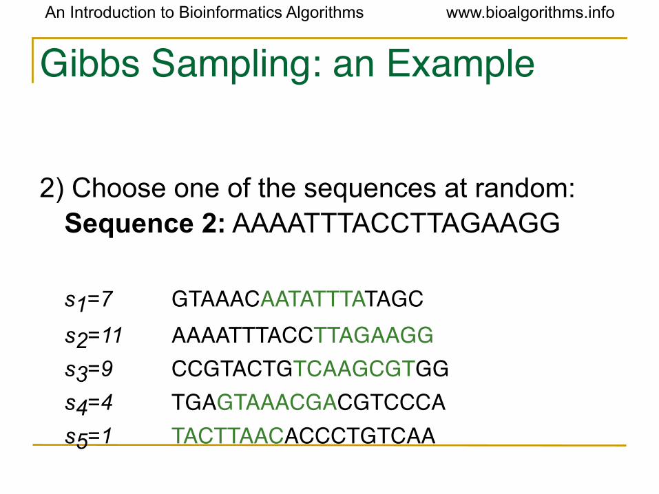
2) Choose one of the sequences at random:Sequence 2: AAAATTTACCTTAGAAGG
s1=7 GTAAACAATATTTATAGCs2=11 AAAATTTACCTTAGAAGGs3=9 CCGTACTGTCAAGCGTGGs4=4 TGAGTAAACGACGTCCCAs5=1 TACTTAACACCCTGTCAA
An Introduction to Bioinformatics Algorithms www.bioalgorithms.info
Gibbs Sampling: an Example
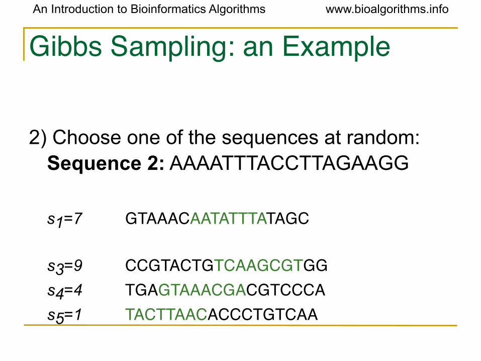
2) Choose one of the sequences at random:Sequence 2: AAAATTTACCTTAGAAGG
s1=7 GTAAACAATATTTATAGC
s3=9 CCGTACTGTCAAGCGTGGs4=4 TGAGTAAACGACGTCCCAs5=1 TACTTAACACCCTGTCAA
An Introduction to Bioinformatics Algorithms www.bioalgorithms.info
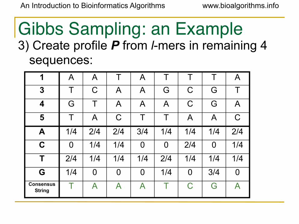
Gibbs Sampling: an Example3) Create profile P from l-mers in remaining 4
sequences:1 A A T A T T T A
3 T C A A G C G T
4 G T A A A C G A
5 T A C T T A A C
A 1/4 2/4 2/4 3/4 1/4 1/4 1/4 2/4
C 0 1/4 1/4 0 0 2/4 0 1/4
T 2/4 1/4 1/4 1/4 2/4 1/4 1/4 1/4
G 1/4 0 0 0 1/4 0 3/4 0Consensus
StringT A A A T C G A
An Introduction to Bioinformatics Algorithms www.bioalgorithms.info
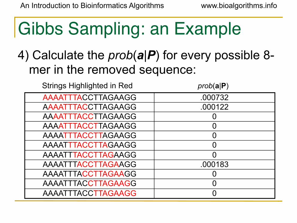
Gibbs Sampling: an Example4) Calculate the prob(a|P) for every possible 8-
mer in the removed sequence:
Strings Highlighted in Red prob(a|P)
AAAATTTACCTTAGAAGG .000732AAAATTTACCTTAGAAGG .000122AAAATTTACCTTAGAAGG 0AAAATTTACCTTAGAAGG 0AAAATTTACCTTAGAAGG 0AAAATTTACCTTAGAAGG 0AAAATTTACCTTAGAAGG 0AAAATTTACCTTAGAAGG .000183AAAATTTACCTTAGAAGG 0AAAATTTACCTTAGAAGG 0AAAATTTACCTTAGAAGG 0
An Introduction to Bioinformatics Algorithms www.bioalgorithms.info
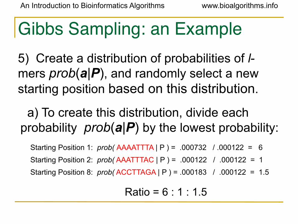
Gibbs Sampling: an Example5) Create a distribution of probabilities of l-mers prob(a|P), and randomly select a new starting position based on this distribution.
Starting Position 1: prob( AAAATTTA | P ) = .000732 / .000122 = 6
Starting Position 2: prob( AAATTTAC | P ) = .000122 / .000122 = 1
Starting Position 8: prob( ACCTTAGA | P ) = .000183 / .000122 = 1.5
a) To create this distribution, divide each probability prob(a|P) by the lowest probability:
Ratio = 6 : 1 : 1.5
An Introduction to Bioinformatics Algorithms www.bioalgorithms.info
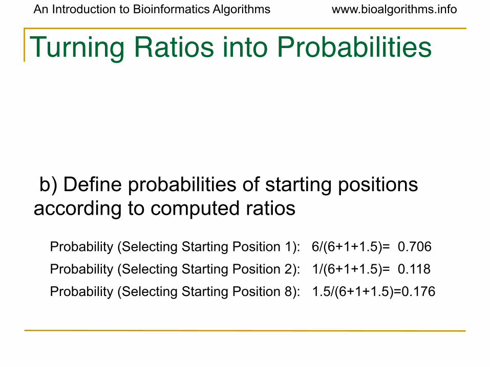
Turning Ratios into Probabilities
Probability (Selecting Starting Position 1): 6/(6+1+1.5)= 0.706
Probability (Selecting Starting Position 2): 1/(6+1+1.5)= 0.118
Probability (Selecting Starting Position 8): 1.5/(6+1+1.5)=0.176
b) Define probabilities of starting positions according to computed ratios
An Introduction to Bioinformatics Algorithms www.bioalgorithms.info
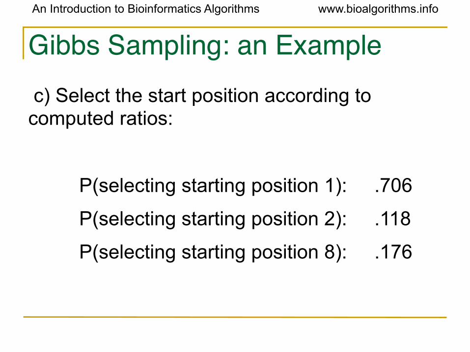
Gibbs Sampling: an Example c) Select the start position according to computed ratios:
P(selecting starting position 1): .706
P(selecting starting position 2): .118
P(selecting starting position 8): .176
An Introduction to Bioinformatics Algorithms www.bioalgorithms.info
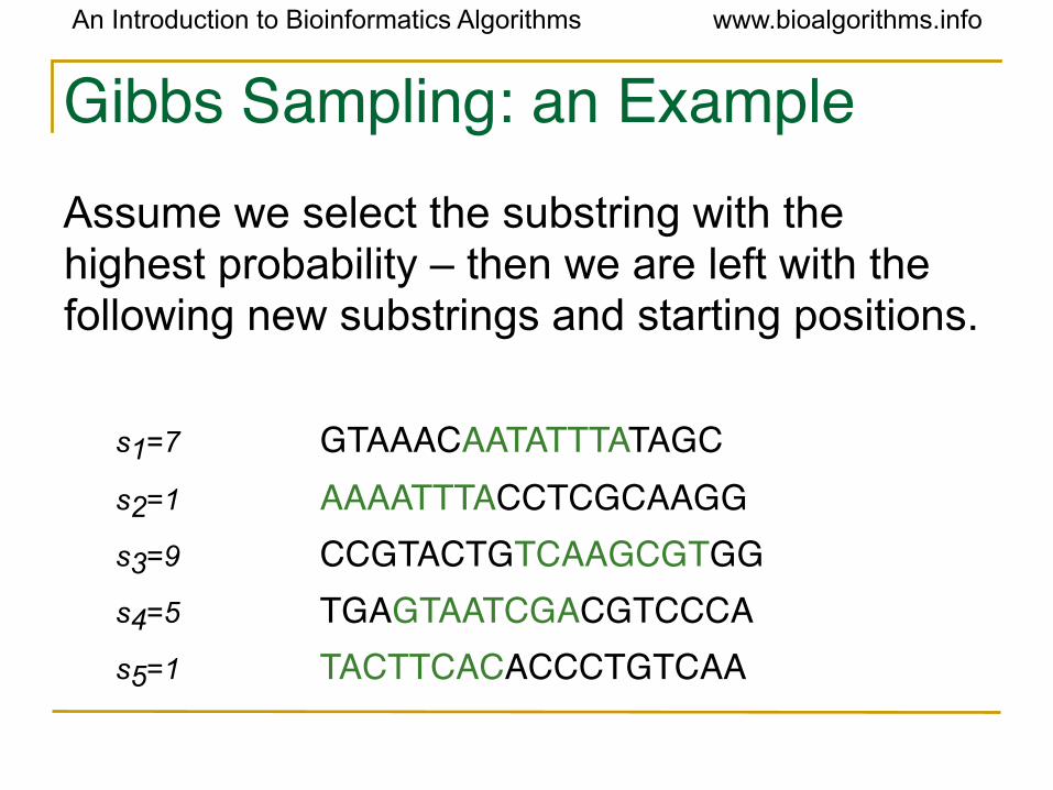
Gibbs Sampling: an ExampleAssume we select the substring with the highest probability – then we are left with the following new substrings and starting positions.
s1=7 GTAAACAATATTTATAGCs2=1 AAAATTTACCTCGCAAGGs3=9 CCGTACTGTCAAGCGTGGs4=5 TGAGTAATCGACGTCCCAs5=1 TACTTCACACCCTGTCAA
An Introduction to Bioinformatics Algorithms www.bioalgorithms.info
Gibbs Sampling: an Example6) We iterate the procedure again with the
above starting positions until we cannot improve the score any more.
An Introduction to Bioinformatics Algorithms www.bioalgorithms.info
Gibbs Sampler in Practice• Gibbs sampling needs to be modified when
applied to samples with unequal distributions of nucleotides (relative entropy approach).
• Gibbs sampling often converges to locally optimal motifs rather than globally optimal motifs.
• Needs to be run with many randomly chosen seeds to achieve good results.
An Introduction to Bioinformatics Algorithms www.bioalgorithms.info
Another Randomized Approach• Random Projection Algorithm is a different
way to solve the Motif Finding Problem.• Guiding principle: Some instances of a motif
agree on a subset of positions.• However, it is unclear how to find these “non-
mutated” positions.• To bypass the effect of mutations within a motif,
we randomly select a subset of positions in the pattern creating a projection of the pattern.
• Search for that projection in a hope that the selected positions are not affected by mutations in most instances of the motif.
An Introduction to Bioinformatics Algorithms www.bioalgorithms.info
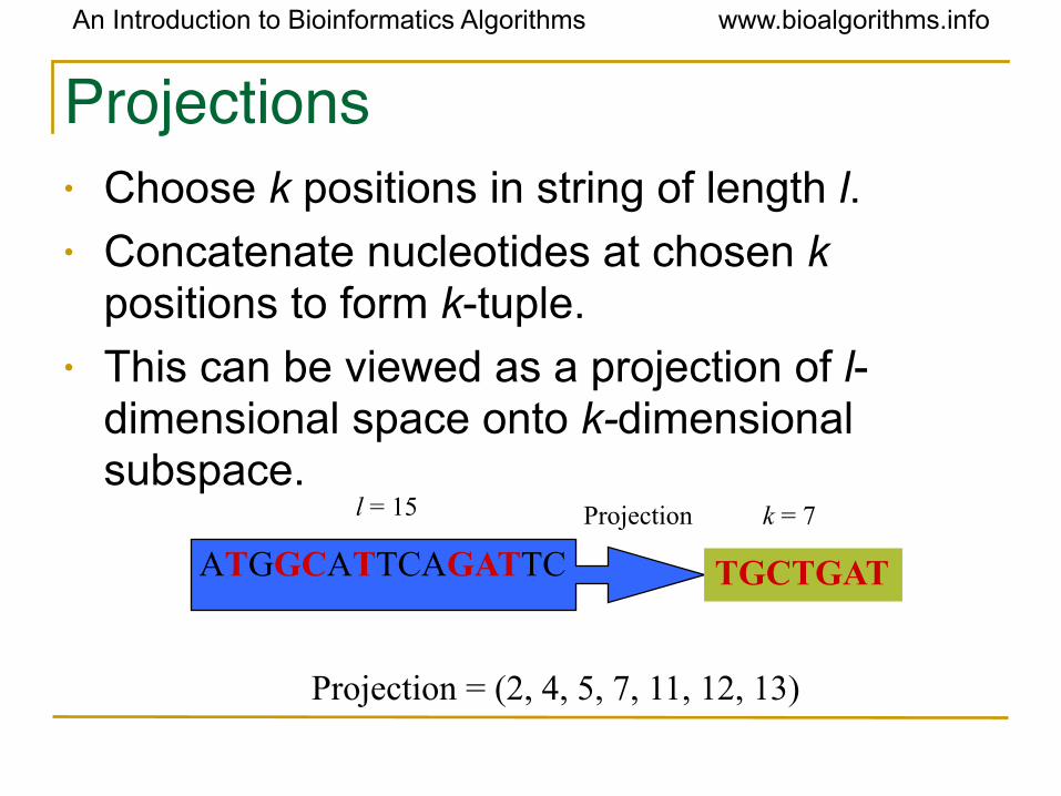
Projections• Choose k positions in string of length l.• Concatenate nucleotides at chosen k
positions to form k-tuple.• This can be viewed as a projection of l-
dimensional space onto k-dimensional subspace.
ATGGCATTCAGATTC TGCTGAT
l = 15 k = 7 Projection
Projection = (2, 4, 5, 7, 11, 12, 13)
An Introduction to Bioinformatics Algorithms www.bioalgorithms.info
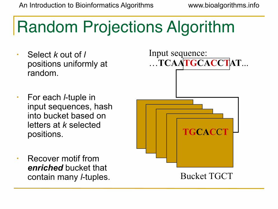
Random Projections Algorithm• Select k out of l
positions uniformly at random.
• For each l-tuple in input sequences, hash into bucket based on letters at k selected positions.
• Recover motif from enriched bucket that contain many l-tuples. Bucket TGCT
TGCACCT
Input sequence:…TCAATGCACCTAT...
An Introduction to Bioinformatics Algorithms www.bioalgorithms.info
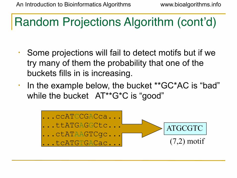
Random Projections Algorithm (cont’d)
• Some projections will fail to detect motifs but if we try many of them the probability that one of the buckets fills in is increasing.
• In the example below, the bucket **GC*AC is “bad” while the bucket AT**G*C is “good”
ATGCGTC
...ccATCCGACca...
...ttATGAGGCtc...
...ctATAAGTCgc...
...tcATGTGACac... (7,2) motif
An Introduction to Bioinformatics Algorithms www.bioalgorithms.info
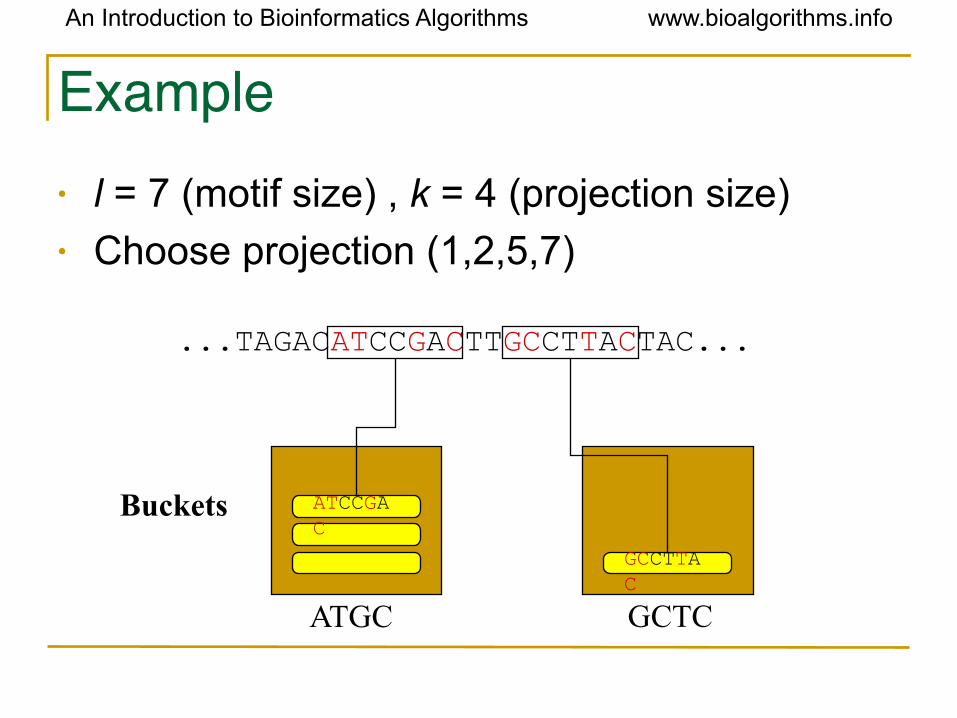
Example• l = 7 (motif size) , k = 4 (projection size)• Choose projection (1,2,5,7)
GCTC
...TAGACATCCGACTTGCCTTACTAC...
Buckets
ATGC
ATCCGAC
GCCTTAC
An Introduction to Bioinformatics Algorithms www.bioalgorithms.info
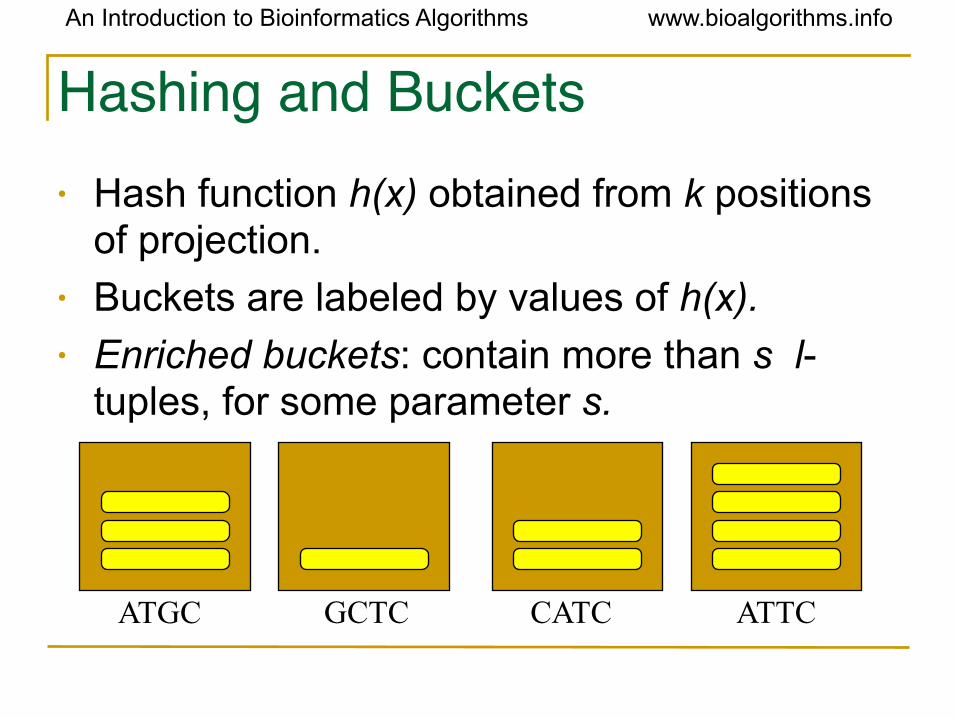
Hashing and Buckets• Hash function h(x) obtained from k positions
of projection. • Buckets are labeled by values of h(x).• Enriched buckets: contain more than s l-
tuples, for some parameter s.
ATTCCATCGCTCATGC

An Introduction to Bioinformatics Algorithms www.bioalgorithms.info
Motif Refinement• How do we recover the motif from the sequences
in the enriched buckets?• k nucleotides are from hash value of bucket.• Use information in other l-k positions as starting
point for local refinement scheme, e.g. Gibbs sampler.
Local refinement algorithmATGCGAC
Candidate motif
ATGC
ATCCGACATGAGGCATAAGTCATGCGAC
An Introduction to Bioinformatics Algorithms www.bioalgorithms.info
Synergy between Random Projection and Gibbs Sampler• Random Projection is a procedure for finding good
starting points: every enriched bucket is a potential starting point.
• Feeding these starting points into existing algorithms (like Gibbs sampler) provides good local search in vicinity of every starting point.
• These algorithms work particularly well for “good” starting points.
An Introduction to Bioinformatics Algorithms www.bioalgorithms.info
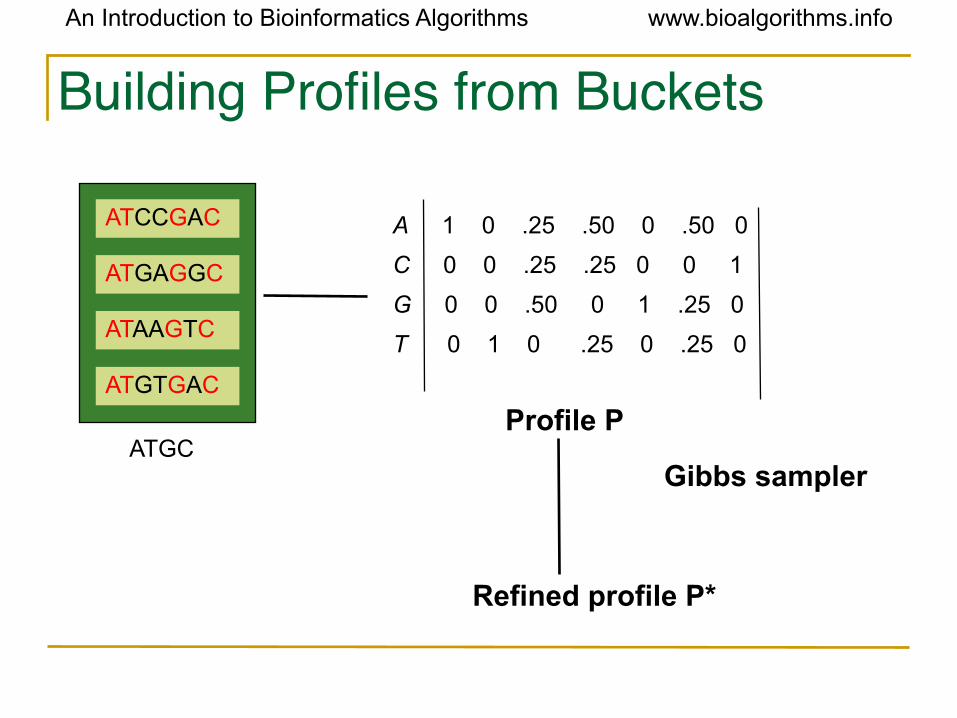
Building Profiles from Buckets
A 1 0 .25 .50 0 .50 0
C 0 0 .25 .25 0 0 1
G 0 0 .50 0 1 .25 0
T 0 1 0 .25 0 .25 0
Profile P
Gibbs sampler
Refined profile P*
ATCCGAC
ATGAGGC
ATAAGTC
ATGTGAC
ATGC
An Introduction to Bioinformatics Algorithms www.bioalgorithms.info
Motif Refinement• For each bucket h containing more than s
sequences, form profile P(h)
• Use Gibbs sampler algorithm with starting point P(h) to obtain refined profile P*
An Introduction to Bioinformatics Algorithms www.bioalgorithms.info
Random Projection Algorithm: A Single Iteration• Choose a random k-projection.• Hash each l-mer x in input sequence into bucket
labeled by h(x)• From each enriched bucket (e.g., a bucket with
more than s sequences), form profile P and perform Gibbs sampler motif refinement
• Candidate motif is best found by selecting the best motif among refinements of all enriched buckets.
An Introduction to Bioinformatics Algorithms www.bioalgorithms.info
Choosing Projection Size• Projection size k
- choose k small enough so that several motif instances hash to the same bucket.
- choose k large enough to avoid contamination by spurious l-mers:
4k >> t (n - l + 1)
An Introduction to Bioinformatics Algorithms www.bioalgorithms.info
How Many Iterations?• Planted bucket : bucket with hash value h(M), where M
is the motif.• Choose m = number of iterations, such that
Pr(planted bucket contains at least s sequences
in at least one of m iterations) =0.95
• Probability is readily computable since iterations form a sequence of independent Bernoulli trials
An Introduction to Bioinformatics Algorithms www.bioalgorithms.info
• S = { x(1),…x(t)} : set of input sequences• Given: A probabilistic motif model W( Q ) depending
on unknown parameters Q, and a background probability distribution P.
• Find value Q max that maximizes likelihood ratio:
• EM is local optimization scheme. Requires starting value Q0.
Expectation Maximization (EM)
Pr(S | W (Q max), P )
Pr(S | P)
An Introduction to Bioinformatics Algorithms www.bioalgorithms.info
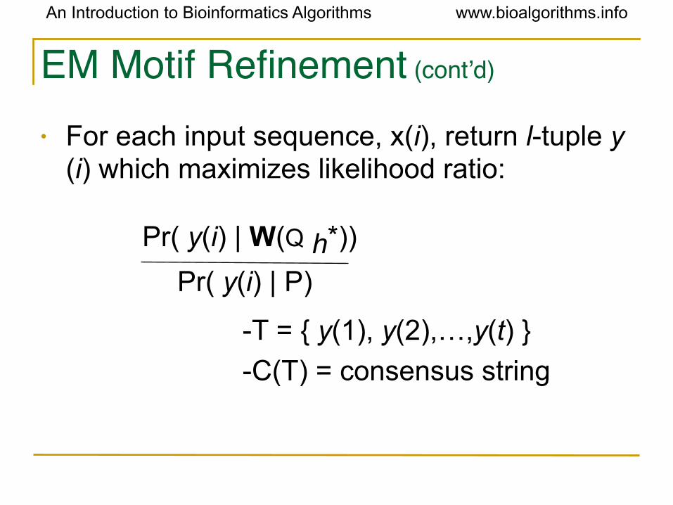
EM Motif Refinement (cont’d)
• For each input sequence, x(i), return l-tuple y(i) which maximizes likelihood ratio:
-T = { y(1), y(2),…,y(t) }
-C(T) = consensus string
Pr( y(i) | W(Q h*))
Pr( y(i) | P)