Random effects structure for confirmatory hypothesistesting: Keep it maximal

Dale J. Barra,∗, Roger Levyb, Christoph Scheepersa, Harry J. Tilyc

aInstitute of Neuroscience and PsychologyUniversity of Glasgow

58 Hillhead St.Glasgow G12 8QBUnited Kingdom

bDepartment of LinguisticsUniversity of California at San Diego

La Jolla, CA 92093-0108USA

cDepartment of Brain and Cognitive SciencesMassachussetts Institute of Technology

Cambridge, MA 02139USA

Abstract

Linear mixed-effects models (LMEMs) have become increasingly prominent in psy-cholinguistics and related areas. However, many researchers do not seem to appreci-ate how random effects structures affect the generalizability of an analysis. Here, weargue that researchers using LMEMs for confirmatory hypothesis testing should min-imally adhere to the standards that have been in place for many decades. Throughtheoretical arguments and Monte Carlo simulation, we show that LMEMs generalizebest when they include the maximal random effects structure justified by the design.The generalization performance of LMEMs including data-driven random effects struc-tures strongly depends upon modeling criteria and sample size, yielding reasonable re-sults on moderately-sized samples when conservative criteria are used, but with littleor no power advantage over maximal models. Finally, random-intercepts-only LMEMsused on within-subjects and/or within-items data from populations where subjects and/oritems vary in their sensitivity to experimental manipulations always generalize worse

∗Corresponding author; Tel: +44 (0)141-330-1602; Fax: +44 (0)141-330-4606.Email addresses: dale.barr@glasgow.ac.uk (Dale J. Barr), rlevy@ucsd.edu (Roger

Levy), christoph.scheepers@glasgow.ac.uk (Christoph Scheepers), hjt@mit.edu(Harry J. Tily)Preprint submitted to Journal of Memory and Language (in press) November 8, 2012

than separate F1 and F2 tests, and in many cases, even worse than F1 alone. MaximalLMEMs should be the ‘gold standard’ for confirmatory hypothesis testing in psycholin-guistics and beyond.

Keywords: linear mixed-effects models, generalization, statistics, Monte Carlosimulation

"I see no real alternative, in most confirmatory studies, to havinga single main question—in which a question is specified by ALL ofdesign, collection, monitoring, AND ANALYSIS."Tukey (1980), “We Need Both Exploratory and Confirmatory” (p.24, emphasis in original).

The notion of independent evidence plays no less important a role in theassessment of scientific hypotheses than it does in everyday reasoning. Considera pet-food manufacturer determining which of two new gourmet cat-food recipesto bring to market. The manufacturer has every interest in choosing the recipethat the average cat will eat the most of. Thus every day for a month (twenty-eight days) their expert, Dr. Nyan, feeds one recipe to a cat in the morning andthe other recipe to a cat in the evening, counterbalancing which recipe is fedwhen and carefully measuring how much was eaten at each meal. At the endof the month Dr. Nyan calculates that recipes 1 and 2 were consumed to thetune of 92.9±5.6 and 107.2±6.1 (means ± S Ds) grams per meal respectively.How confident can we be that recipe 2 is the better choice to bring to market?Without further information you might hazard the guess “somewhat confident”,considering that one of the first statistical hypothesis tests typically taught, theunpaired t-test, gives p = 0.09 against the null hypothesis that choice of recipedoes not matter. But now we tell you that only seven cats participated in thistest, one for each day of the week. How does this change your confidence in thesuperiority of recipe 2?

Let us first take a moment to consider precisely what it is about this new in-formation that might drive us to change our analysis. The unpaired t-test is basedon the assumption that all observations are conditionally independent of one an-other given the true underlying means of the two populations—here, the averageamount a cat would consume of each recipe in a single meal. Since no two catsare likely to have identical dietary proclivities, multiple measurements from the

2

same cat would violate this assumption. The correct characterization becomesthat all observations are conditionally independent of one another given (a) thetrue palatibility effect of recipe 1 versus recipe 2, together with (b) the dietaryproclivities of each cat. This weaker conditional independence is a double-edgedsword. On the one hand, it means that we have tested effectively fewer individu-als than our 56 raw data points suggest, and this should weaken our confidence ingeneralizing the superiority of recipe 2 to the entire cat population. On the otherhand, the fact that we have made multiple measurements for each cat holds outthe prospect of factoring out each cat’s idiosyncratic dietary proclivities as partof the analysis, and thereby improving the signal-to-noise ratio for inferencesregarding each recipe’s overall appeal. How we specify these idiosyncrasies candramatically affect our conclusions. For example, we know that some cats havehigher metabolisms and will tend to eat more at every meal than other cats. Butwe also know that each creature has its own palate, and even if the recipes wereof similar overall quality, a given cat might happen to like one recipe more thanthe other. Indeed, accounting for idiosyncratic recipe preferences for each catmight lead to even weaker evidence for the superiority of recipe 2.

Situations such as these, where individual observations cluster together viaassociation with a smaller set of entities, are ubiquitous in psycholinguistics andrelated fields—where the clusters are typically human participants and stimulusmaterials (i.e., items). Similar clustered-observation situations arise in other sci-ences, such as agriculture (plots in a field) and sociology (students in classroomsin schools in school-districts); hence accounting for the random effects of theseentities has been an important part of the workhorse statistical analysis tech-nique, the analysis of variance, under the name mixed-model ANOVA, since thefirst half of the twentieth century (Fisher, 1925; Scheffe, 1959). In experimentalpsychology, the prevailing standard for a long time has been to assume that indi-vidual participants may have idiosyncratic sensitivities to any experimental ma-nipulation that may have an overall effect, so detecting a “fixed effect” of somemanipulation must be done under the assumption of corresponding participantrandom effects for that manipulation as well. In our pet-food example, if there isa true effect of recipe—that is, if on average a new, previously unstudied cat willon average eat more of recipe 2 than of recipe 1—it should be detectable aboveand beyond the noise introduced by cat-specific recipe preferences, provided wehave enough data. Technically speaking, the fixed effect is tested against an errorterm that captures the variability of the effect across individuals.

Standard practices for data-analysis in psycholinguistics and related areasfundamentally changed, however, after Clark (1973). In a nutshell, Clark (1973)

3

argued that linguistic materials, just like experimental participants, have idiosyn-crasies that need to be accounted for. Because in a typical psycholinguistic ex-periment, there are multiple observations for the same item (e.g., a given word orsentence), these idiosyncrasies break the conditional independence assumptionsunderlying mixed-model ANOVA, which treats experimental participant as theonly random effect. Clark proposed the quasi-F (F′) and min-F′ statistics asapproximations to an F-ratio whose distributional assumptions are satisfied evenunder what in contemporary parlance is called crossed random effects of partic-ipant and item (Baayen et al., 2008). Clark’s paper helped drive the field towarda standard demanding evidence that experimental results generalized beyond thespecific linguistic materials used—in other words, the so-called by-subjects F1

mixed-model ANOVA was not enough. There was even a time where report-ing of the min-F′ statistic was made a standard for publication in the Journalof Memory and Language. However, acknowledging the widespread belief thatmin-F′ is unduly conservative (see, e.g., Forster & Dickinson, 1976), signifi-cance of min-F′ was never made a requirement for acceptance of a publication.Instead, the ‘normal’ convention continued to be that a result is considered likelyto generalize if it passes p < 0.05 significance in both by-subjects (F1) andby-items (F2) ANOVAs. In the literature this criterion is called F1 × F2 (e.g.,Forster & Dickinson, 1976), which in this paper we use to denote the larger (lesssignificant) of the two p values derived from F1 and F2 analyses.

Linear Mixed-Effects Models (LMEMs)Since Clark (1973), the biggest change in data analysis practices has been the

introduction of methods for simultaneously modeling crossed participant anditem effects in a single analysis, in what is variously called “hierarchical re-gression”, “multi-level regression”, or simply “mixed-effects models” (Baayen,2008; Baayen et al., 2008; Gelman & Hill, 2007; Goldstein, 1995; Kliegl, 2007;Locker et al., 2007; Pinheiro & Bates, 2000; Quené & van den Bergh, 2008;Snijders & Bosker, 1999b).1 In this paper we refer to models of this class asmixed-effects models; when fixed effects, random effects, and trial-level noise

1Despite the “mixed-effects models” nomenclature, traditional ANOVA approaches used inpsycholinguistics have always used “mixed effects” in the sense of simultaneously estimatingboth fixed- and random-effects components of such a model. What is new about mixed effectsmodels is their explicit estimation of the random-effects covariance matrix, which leads to con-siderably greater flexibility of application, including, as clearly indicated by the title of Baayenet al. (2008), the ability to handle the crossing of two or more types of random effects in a singleanalysis.

4

contribute linearly to the dependent variable, and random effects and trial-levelerror are both normally distributed and independent for differing clusters or tri-als, it is a linear mixed-effects model (LMEM).

The ability of LMEMs to simultaneously handle crossed random effects, inaddition to a number of other advantages (such as better handling of categoricaldata; see Dixon, 2008; Jaeger, 2008), has given them considerable momentumas a candidate to replace ANOVA as the method of choice in psycholinguisticsand related areas. But despite the widespread use of LMEMs, there seems tobe insufficently widespread understanding of the role of random effects in suchmodels, and very few standards to guide how random effect structures should bespecified for the analysis of a given dataset. Of course, what standards are ap-propriate or inappropriate depends less upon the actual statistical technique beingused, and more upon the goals of the analysis (cf. Tukey, 1980). Ultimately, therandom effect structure one uses in an analysis encodes the assumptions that onemakes about how sampling units (subjects and items) vary, and the structure ofdependency that this variation creates in one’s data.

In this paper, our focus is mainly on what assumptions about sampling unitvariation are most critical for the use of LMEMs in confirmatory hypothesis test-ing. By confirmatory hypothesis testing we mean the situation in which theresearcher has identified a specific set of theory-critical hypotheses in advanceand attempts to measure the evidence for or against them as accurately as pos-sible (Tukey, 1980). Confirmatory analyses should be performed according toa principled plan guided by theoretical considerations, and, to the extent possi-ble, should minimize the influence of the observed data on the decisions that onemakes in the analysis (Wagenmakers et al., in press). To simplify our discussion,we will focus primarily on the confirmatory analysis of simple data sets involv-ing only a few theoretically-relevant variables. We recognize that in practice, thecomplexity of one’s data may impose constraints on the extent to which one canperform analyses fully guided by theory and not by the data. Researchers whoperform laboratory experiments have extensive control over the data collectionprocess, and, as a result, their statistical analyses tend to include only a small setof theoretically relevant variables, because other extraneous factors have beenrendered irrelevant through randomization and counterbalancing. This is in con-trast to other more complex types of data sets, such as observational corpora orlarge-scale data sets collected in the laboratory for some other, possibly moregeneral, purpose than the theoretical question at hand. Such datasets may beunbalanced and complex, and include a large number of measurements of manydifferent kinds. Analyzing such datasets appropriately is likely to require more

5

sophisticated statistical techniques than those we discuss in this paper. Further-more, such analyses may involve data-driven techniques typically used in ex-ploratory data analysis in order to reduce the set of variables to a manageablesize. Discussion of such techniques for complex datasets and their proper appli-cation of is beyond the scope of this paper (but see, e.g., Baayen, 2008; Jaeger,2010).

Our focus here is on the question: When the goal of a confirmatory analysisis to test hypotheses about one or more critical “fixed effects”, what random-effects structure should one use? Based on theoretical analysis and Monte Carlosimulation, we will argue the following:

1. Implicit choices regarding random-effect structures existed for traditionalmixed-model ANOVAs just as they exist today for LMEMs;

2. With mixed-model ANOVAs, the standard has been to use what we term“maximal” random-effect structures;

3. Insofar as we as a field think this standard is appropriate for the purposeof confirmatory hypothesis testing, researchers using LMEMs for that pur-pose should also be using LMEMs with maximal random effects structure;

4. Failure to include maximal random-effect structures in LMEMs (whensuch random effects are present in the underlying populations) inflatesType I error rates;

5. For designs including within-subjects (or within-items) manipulations,random-intercepts-only LMEMs can have catastrophically high Type I er-ror rates, regardless of how p-values are computed from them (see alsoRoland, 2009; Jaeger, 2011a; and Schielzeth & Forstmeier, 2009);

6. The performance of a data-driven approach to determining random effects(i.e., model selection) depends strongly on the specific algorithm, size ofthe sample, and criteria used; moreover, the power advantage of this ap-proach over maximal models is typically negligible;

7. In terms of power, maximal models perform surprisingly well even in a“worst case” scenario where they assume random slope variation that isactually not present in the population;

8. Contrary to some warnings in the literature (Pinheiro & Bates, 2000),likelihood-ratio tests for fixed effects in LMEMs show minimal Type Ierror inflation for psycholinguistic datasets (see Baayen et al., 2008, Foot-note 1, for a similar suggestion); also, deriving p-values from Monte CarloMarkov Chain (MCMC) sampling does not mitigate the high Type I errorrates of random-intercepts-only LMEMs;

6

9. The F1 × F2 criterion leads to increased Type I error rates the more theeffects vary across subjects and items in the underlying populations (seealso Clark, 1973; Forster & Dickinson, 1976);

10. Min-F′ is conservative in between-items designs when the item varianceis low, and is conservative overall for within-items designs, especially sowhen the treatment-by-subject and/or treatment-by-item variances are low(see also Forster & Dickinson, 1976); in contrast, maximal LMEMs showno such conservativity.

Further results and discussion are available in an online appendix (http://talklab.psy.gla.ac.uk/simgen).

Random effects in LMEMs and ANOVA: The same principles applyThe Journal of Feline Gastronomy has just received a submission reporting

that the feline palate prefers tuna to liver, and as journal editor you must de-cide whether to send it out for review. The authors report a highly significanteffect of recipe type (p < .0001), stating that they used “a mixed effects modelwith random effects for cats and recipes”. Are you in a position to evaluate thegenerality of the findings? Given that LMEMs can implement nearly any of thestandard parametric tests—from a one-sample test to a multi-factor mixed-modelANOVA—the answer can only be no. Indeed, whether LMEMs produce validinferences depends critically on how they are used. What you need to know inaddition is the random effects structure of the model, because this is what the as-sessment of the treatment effects is based on. In other words, you need to knowwhich treatment effects are assumed to vary across which sampled units, and howthey are assumed to vary. As we will see, whether one is specifying a randomeffects structure for LMEMs or choosing an analysis from among the traditionaloptions, the same considerations come into play. So, if you are scrupulous aboutchoosing the “right” statistical technique, then you should be equally scrupulousabout using the “right” random effects structure in LMEMs. In fact, knowinghow to choose the right test already puts you in a position to specify the correctrandom effects structure for LMEMs.

In this section, we attempt to distill the implicit standards already in placeby walking through a hypothetical example and discussing the various modelsthat could be applied, their underlying assumptions, and how these assumptionsrelate to more traditional analyses. In this hypothetical “lexical decision” experi-ment, subjects see strings of letters and have to decide whether or not each stringforms an English word, while their response times are measured. Each subjectis exposed to two types of words, forming condition A and condition B of the

7

experiment. The words in one condition differ from those in the other condi-tion on some intrinsic categorical dimension (e.g., syntactic class), comprising aword-type manipulation that is within-subjects and between-items. The questionis whether reaction times are systematically different between condition A andcondition B. For expository purposes, we use a “toy” dataset with hypotheticaldata from four subjects and four items, yielding two observations per treatmentcondition per participant. The observed data are plotted alongside predictionsfrom the various models we will be considering in the panels of Figure 1. Be-cause we are using simulated data, all of the parameters of the population areknown, as well as the “true” subject-specific and item-specific effects for thesampled data. In practice, researchers do not know these values and can onlyestimate them from the data; however, using known values for hypothetical datacan aid in understanding how clustering in the population maps onto clusteringin the sample.

Figure 1: Example RT data (open symbols) and model predictions (filled symbols) for a hypo-thetical lexical decision experiment with two within-subject/between-item conditions, A (trian-gles) and B (circles), including four subjects (S1-S4) and four items (I1-I4). Panel (a) illustratesa model with no random effects, considering only the baseline average RT (response to word typeA) and treatment effect; panel (b) adds random subject intercepts to the model; panel (c) addsby-subject random slopes; and panel (d) illustrates the additional inclusion of by-item randomintercepts. Panel (d) represents the maximal random-effects structure justified for this design;any remaining discrepancies between observed data and model estimates are due to trial-levelmeasurement error (esi).

8

The general pattern for the observed data points suggests that items of typeB (I3 and I4) are responded to faster than items of type A (I1 and I2). Thissuggests a simple (but clearly inappropriate) model for these data that relatesresponse Ysi for subject s and item i to a baseline level via fixed-effect β0 (theintercept), a treatment effect via fixed-effect β1 (the slope), and observation-levelerror esi with variance σ2:

Ysi = β0 + β1Xi + esi, (1)

esi ∼ N(0, σ2

)where Xi is a predictor variable2 taking on the value of 0 or 1 depending onwhether item i is of type A or B respectively, and esi ∼ N

(0, σ2

)indicates that

the trial-level error is normally distributed with mean 0 and variance σ2. In thepopulation, participants respond to items of type B 40 ms faster than items oftype A. Under this first model, we assume that each of the 16 observations pro-vides the same evidence for or against the treatment effect regardless of whetheror not any other observations have already been taken into account. Performingan unpaired t-test on these data would implicitly assume this (incorrect) genera-tive model.

Model (1) is not a mixed-effects model because we have not defined anysources of clustering in our data; all observations are conditionally independentgiven a choice of intercept, treatment effect, and noise level. But experience tellsus that different subjects are likely to have different overall response latencies,breaking conditional independence between trials for a given subject. We canexpand our model to account for this by including a new offset term S 0s, thedeviation from β0 for subject s. The expanded model is now

Ysi = β0 + S 0s + β1Xi + esi, (2)

S 0s ∼ N(0, τ00

2),

esi ∼ N(0, σ2

).

2For expository purposes, we use a treatment coding scheme (0 or 1) for the predictor vari-able. Alternatively, the models in this section could be expressed in the style more common totraditional ANOVA pedagogy, where fixed and random effects represent deviations from a grandmean. This model can be fit by using “deviation coding” for the predictor variable (-.5 and .5instead of 0 and 1). For higher-order designs, treatment and deviation coding schemes will leadto different interpretations for lower-order effects (simple effects for contrast coding and maineffects for deviation coding).

9

These offsets increase the model’s expressivity by allowing predictions for eachsubject to shift upward or downward by a fixed amount (Figure 1b). Our useof Latin letters for this term is a reminder that S 0s is a special type of effectwhich is different from the βs—indeed, we now have a “mixed-effects” model:parameters β0 and β1 are fixed effects (effects that are assumed to be constantfrom one experiment to another), while the specific composition of subject levelsfor a given experiment is assumed to be a random subset of the levels in theunderlying populations (another instantiation of the same experiment would havea different composition of subjects, and therefore different realizations of theS 0s effects). The S 0s effects are therefore random effects; specifically, they arerandom intercepts, as they allow the intercept term to vary across subjects. Ourprimary goal is to produce a model which will generalize to the population fromwhich these subjects are randomly drawn, rather than describing the specific S 0s

values for this sample. Therefore, instead of estimating the individual S 0s effects,the model-fitting algorithm estimates the population distribution from which theS 0s effects were drawn. This requires assumptions about this distribution; wefollow the common assumption that it is normal, with a mean of 0 and a varianceof τ00

2; here τ002 is a random effect parameter, and is denoted by a Greek symbol

because, like the βs, it refers to the population and not to the sample.Note that the variation on the intercepts is not confounded with our effect

of primary theoretical interest (β1): for each subject, it moves the means forboth conditions up or down by a fixed amount. Accounting for this variationwill typically decrease the residual error and thus increase the sensitivity of thetest of β1. Fitting Model (2) is thus analogous to analyzing the raw, unaggregatedresponse data using a repeated-measures ANOVA with S S sub jects subtracted fromthe residual S S error term. One could see that this analysis is wrong by observingthat the denominator degrees of freedom for the F statistic (i.e., correspondingto MS error) would be greater than the number of subjects (see online appendixfor further discussion and demonstration).

Although Model (2) is clearly preferable to Model (1), it does not captureall the possible by-subject dependencies in the sample; experience also tells usthat subjects often vary not only in their overall response latencies but also in thenature of their response to word type. In the present hypothetical case, Subject 3shows a total effect of 134 ms, which is 94 ms larger than the average effect in thepopulation of 40 ms. We have multiple observations per combination of subjectand word type, so this variability in the population will also create clusteringin the sample. The S0s do not capture this variability because they only allowsubjects to vary around β0. What we need in addition are random slopes to allow

10

subjects to vary with respect to β1, our treatment effect. To account for thisvariation, we introduce a random slope term S 1s with variance τ11

2, yielding

Ysi = β0 + S 0s + (β1 + S 1s)Xi + esi, (3)

(S 0s, S 1s) ∼ N(0,

[τ00

2 ρτ00τ11

ρτ00τ11 τ112

]),

esi ∼ N(0, σ2

).

This is now a mixed-effects model with by-subject random intercepts and ran-dom slopes. Note that the inclusion of the by-subject random slope causes thepredictions for condition B to shift by a fixed amount for each subject (Fig-ure 1c), improving predictions for words of type B. The slope offset S 1s captureshow much Subject s’s effect deviates from the population treatment effect β1.Again, we do not want our analysis to commit to particular S 1s effects, and so,rather than estimating these values directly, we estimate τ11

2, the by-subject vari-ance in treatment effect. But note that now we have two random effects for eachsubject s, and these two effects can exhibit a correlation (expressed by ρ). Forexample, subjects who do not read carefully might not only respond faster thanthe typical subject (and have a negative S0s), but might also show less sensitivityto the word type manipulation (and have a more positive S1s). Indeed, such a neg-ative correlation, where we would have ρ < 0, is suggested in our hypotheticaldata (Figure 1): S1 and S3 are slow responders who show clear treatment effects,whereas S2 and S4 are fast responders who are hardly susceptible to the wordtype manipulation. In the most general case, we should not treat these effectsas coming from independent univariate distributions, but instead should treat S 0s

and S 1s as being jointly drawn from a bivariate distribution. As seen in line 2of Equation 3, we follow common assumptions in taking this distribution as bi-variate normal with a mean of (0, 0) and three free parameters: τ00

2 (random in-tercept variance), τ11

2 (random slope variance), and ρτ00τ11 (the intercept/slopecovariance). For further information about random effect variance-covariancestructures, see Baayen (2004, 2008); Gelman & Hill (2007); Goldstein (1995);Raudenbush & Bryk (2002); Snijders & Bosker (1999a).

Both Models (2) and (3) are instances of what is traditionally analyzed using“mixed-model ANOVA” (e.g., Scheffe, 1959, chapter 8). By long-standing con-vention in our field, however, the classic “by-subjects ANOVA” (and analogously“by-items ANOVA” when items are treated as the random effect) is understood tomean Model (3), the relevant F-statistic for which is F1 = MS T

MS T xS, where MS T is

the treatment mean square and MS T xS is the treatment-by-subject mean square.11

This convention presumably derives from the widespread recognition that sub-jects (and items) usually do vary idiosyncratically not only in their global meanresponses but also in their sensitivity to the experimental treatment. Moreover,this variance, unlike random intercept variance, can drive differences betweencondition means. This can be seen by comparing the contributions of randomintercepts versus random slopes across panels (b) and (c) in Figure 1. Therefore,it would seem to be important to control for such variation when testing for atreatment effect.3

Although Model (3) accounts for all by-subject random variation, it still hasa critical defect. As Clark (1973) noted, the repetition of words across obser-vations is a source of non-independence not accounted for, which would impairgeneralization of our results to new items. We need to incorporate item variabil-ity into the model with the random effects I0i, yielding

Ysi = β0 + S 0s + I0i + (β1 + S 1s)Xi + esi, (4)

(S 0s, S 1s) ∼ N(0,

[τ00

2 ρτ00τ11

ρτ00τ11 τ112

]),

I0i ∼ N(0, ω00

2),

esi ∼ N(0, σ2

).

This is a mixed-effect model with by-subject random intercepts and slopes andby-item random intercepts. Rather than committing to specific I0i values, weassume that the I0i effects are drawn from a normal distribution with a meanof zero and variance ω00

2. We also assume that ω002 is independent from the

τ parameters defining the by-subject variance components. Note that the inclu-sion of by-item random intercepts improves the predictions from the model, withpredictions for a given item shifting by a consistent amount across all subjects(Figure 1d). It is also worth noting that the by-item variance is also confoundedwith our effect of interest, since we have different items in the different condi-tions, and thus will tend to contribute to any difference we observe between thetwo condition means.

3Note that in practice, most researchers do not compute MS T xS on the raw data but ratheraggregate their data first so that there is one observation per subject per cell, and then performan ANOVA (or t-test) on the cell means. This aggregation confounds the random slope variancewith residual error and reduces the error degrees of freedom, making it possible to perform arepeated-measures ANOVA. This is an alternative way of meeting the assumption of conditionalindependence, but the aggregation precludes simultaneous generalization over subjects and items(see online appendix for further details).

12

This analysis has a direct analogue to min-F′, which tests MS T against adenominator term consisting of the sum of MS T xS and MS I , the mean squaresfor the random treatment-by-subject interaction and the random main effect ofitems. It is, however, different from the practice of performing F1 × F2 andrejecting the null hypothesis if p < .05 for both Fs. The reason is that MST

(the numerator for both F1 and F2) reflects not only the treatment effect, butalso treatment-by-subject variability (τ11

2) as well as by-item variability (ω002).

The denominator of F1 controls for treatment-by-subject variability but not itemvariability; similarly, the denominator of F2 controls for item variability but nottreatment-by-subject variability. Thus, finding that F1 is significant implies thatβ1 , 0 or ω00

2 , 0, or both; likewise, finding that F2 is significant implies thatβ1 , 0 or τ11

2 , 0, or both. Since ω002 and τ11

2 can be nonzero while β1 = 0,F1 × F2 tests will inflate the Type I error rate (Clark, 1973). Thus, in termsof controlling Type I error rate, the mixed-effects modeling approach and themin-F′ approach are, at least theoretically, superior to separate by-subject andby-item tests.

At this point, we might wish to go further and consider other models. Forinstance, we have considered a by-subject random slope; for consistency, whydon’t we also consider a model with a by-item random slope, I1i? A little re-flection reveals that a by-item random slope does not make sense for this design.Words are nested within word types—no word can be both type A and type B—so it is not sensible to ask whether words vary in their sensitivity to word type.No sample from this experiment could possibly give us the information neededto estimate random slope variance and random slope/intercept covariance pa-rameters for such a model. A model like this is unidentifiable for the data it isapplied to: there are (infinitely) many different values we could choose for itsparameters which would describe the data equally well.4 Experiments with awithin-item manipulation, such as a priming experiment in which target wordsare held constant across conditions but the prime word is varied, would call forby-item random slopes, but not the current experiment.

The above point also extends to designs where one independent variable ismanipulated within- and another variable between- subjects (respectively items).In case of between-subject manipulations, the levels of the subject variable arenested within the levels of the experimental treatment variable (i.e. each subjectbelongs to one and only one of the experimental treatment groups), meaning that

4Technically, by-item random slopes for a between-item design can be used to capture het-eroscedasticity across conditions, but this is typically a minor concern in comparison with theissues focused on in this paper (see, e.g., discussion in Gelman & Hill, 2007).

13

subject and treatment cannot interact—a model with a by-subject random slopeterm would be unidentifiable. In general, within-unit treatments require boththe by-unit intercepts and slopes in the random effects specification, whereasbetween-unit treatments require only the by-unit random intercepts.

It is important to note that identifiability is a property of the model givena certain dataset. The model with by-item random slopes is unidentifiable forany possible dataset because it tries to model a source of variation that couldnot logically exist in the population. However, there are also situations where amodel is unidentifiable because there is insufficient data to estimate its parame-ters. For instance, we might decide it was important to try to estimate variabilitycorresponding to the different ways that subjects might respond to a given word(a subject-by-item random intercept). But to form a cluster in the sample, it isnecessary to have more than one observation for a given unit; otherwise, the clus-tering effect cannot be distinguished from residual error.5 If we only elicit oneobservation per subject/item combination, we are unable to estimate this sourceof variability, and the model containing this random effect becomes unidentifi-able. Had we used a design with repeated exposures to the same items for agiven subject, the same model would be identifiable, and in fact we would needto include that term to avoid violating the conditional independence of our ob-servations given subject and item effects.

This discussion indicates that Model (4) has the maximal random effectsstructure justified by our experimental design, and we henceforth refer to suchmodels as maximal models. A maximal model should optimize generalizationof the findings to new subjects and new items. Models that lack random ef-fects contained in the maximal model, such as Models (1)-(3), are likely to bemisspecified—the model specification may not be expressive enough to includethe true generative process underlying the data. This type of misspecificationis problematic because conditional independence between observations within agiven cluster is not achieved. Each source of random variation that is not ac-counted for will tend to work against us in one of two different ways. On theone hand, unaccounted-for variation that is orthogonal to our effect of interest(e.g., random intercept variation) will tend to reduce power for our tests of thateffect; on the other, unaccounted-for variation that is confounded with our effectof interest (e.g., random slope variation), can drive differences between means,and thus will tend to increase the risk of Type I error.

5It can also be difficult to estimate random effects when some of the sampling units (subjectsor items) provide few observations in particular cells of the design. See the General Discussionand Jaeger et al. (2011, section 3.3) for further discussion of this issue.

14

A related model that we have not yet considered but that has become popularin recent practice includes only by-subject and by-item random intercepts.

Ysi = β0 + S 0s + I0i + β1Xi + esi, (5)

S 0i ∼ N(0, τ00

2),

I0i ∼ N(0, ω00

2),

esi ∼ N(0, σ2

).

Unlike the other models we have considered up to this point, there is noclear ANOVA analog to a random-intercepts-only LMEM; it is perhaps akin toa modified min-F′ statistic with a denominator error term including MS I butwith MS T xS replaced by the error term from Model 2 (i.e., with S S error reducedby S S sub jects). But it would seem inappropriate to use this as a test statistic,given that the numerator MS T increases as a function not only of the overalltreatment effect, but also as a function of random slope variation (τ11

2), and thedenominator does not control for this variation.

A common misconception is that crossing subjects and items in the interceptterm of LMEMs is sufficient for meeting the assumption of conditional indepen-dence, and that including random slopes is strictly unnecessary unless it is oftheoretical interest to estimate that variability (see e.g., Janssen, 2012; Lockeret al., 2007). However, this is problematic given the the fact that, as alreadynoted, random slope variation can drive differences between condition means,thus creating a spurious impression of a treatment effect where none might exist.Indeed, some researchers have already warned against using random-intercepts-only models when random slope variation is present (e.g., Baayen, 2008; Jaeger,2011a; Roland, 2009; Schielzeth & Forstmeier, 2009). However, the perfor-mance of these models has not yet been evaluated in the context of simultaneousgeneralization over subjects and items. Our simulations will provide such anevaluation.

Although the maximal model best captures all the dependencies in the sam-ple, sometimes it becomes necessary for practical reasons to simplify the randomeffects structure. Fitting LMEMs typically involves maximum likelihood estima-tion, where an iterative procedure is used to come up with the “best” estimatesfor the parameters given the data. As the name suggests, it attempts to maximizethe likelihood of the data given the structure of the model. Sometimes, however,the estimation procedure will fail to “converge” (i.e., to find a solution) withina reasonable number of iterations. The likelihood of this convergence failure

15

tends to increase with the complexity of the model, especially the random effectsstructure.

Ideally, simplification of the random effects structure should be done in aprincipled way. Dropping a random slope is not the only solution, nor is it likelyto be the best, given that random slopes tend to account for variance confoundedwith the fixed effects of theoretical interest. We thus consider two additionalmixed-effects models with simplified random effects structure.6 The first of theseis almost identical to the maximal model (Model 4) but without any correlationparameter:

Ysi = β0 + S 0s + I0i + (β1 + S 1s)Xi + esi, (6)

(S 0s, S 1s) ∼ N(0,

[τ00

2 00 τ11

2

]),

I0i ∼ N(0, ω00

2),

esi ∼ N(0, σ2

).

Note that the only difference from Model 4 is in the specification of the dis-tribution of (S 0s, S 1s) pairs. Model 6 is more restrictive than Model 4 in notallowing correlation between the random slope and random intercept; if, for ex-ample, subjects with overall faster reaction times also tended to be less sensitiveto experimental manipulation (as in our motivating example for random slopes),Model 6 could not capture that aspect of the data. But it does account for thecritical random variances that are confounded with the effect of interest, τ11

2 andω00

2.The next and final model to consider is one that has received almost no dis-

cussion in the literature but is nonetheless logically possible: a maximal modelthat is simplified by removing random intercepts for any within-unit (subject oritem) factor. For the current design, this means removing the by-subject randomintercept:

6Unlike the other models we have considered up to this point, the performance of these twoadditional models (Models 6 and 7) will depend to some extent on how the predictor variable Xis coded (e.g., treatment or deviation coding, with performance generally better for the latter; seeAppendix for further discussion).

16

Table 1: Summary of models considered and associated lmer syntax.No. Model lmer model syntax(1) Ysi = β0 + β1Xi + esi n/a (not a mixed-effects model)(2) Ysi = β0 + S 0s + β1Xi + esi Y∼X+(1|Subject)

(3) Ysi = β0 + S 0s + (β1 + S 1s)Xi + esi Y∼X+(1+X|Subject)

(4) Ysi = β0 + S 0s + I0i + (β1 + S 1s)Xi + esi Y∼X+(1+X|Subject)+(1|Item)

(5) Ysi = β0 + S 0s + I0i + β1Xi + esi Y∼X+(1|Subject)+(1|Item)

(6)∗ As (4), but S 0s, S 1s independent Y∼X+(1|Subject)+(0+X|Subject)+(1|Item)∗

(7)∗ Ysi = β0 + I0i + (β1 + S 1s)Xi + esi Y∼X+(0+X|Subject)+(1|Item)∗

∗Performance is sensitive to the coding scheme for variable X (see Appendix)

Ysi = β0 + I0i + (β1 + S 1s)Xi + esi, (7)

S 1s ∼ N(0, τ11

2),

I0i ∼ N(0, ω00

2),

esi ∼ N(0, σ2

).

This model, like random-intercepts-only and no-correlation models, would al-most certainly be misspecified for typical psycholinguistic data. However, likethe previous model, and unlike the random-intercepts-only model, it capturesall the sources of random variation that are confounded with the effect of maintheoretical interest.

The mixed-effects models considered in this section are presented in Table 1.We give their expression in the syntax of lmer (Bates et al., 2011), a widely usedmixed-effects fitting method for R (R Development Core Team, 2011). To sum-marize, when specifying random effects, one must be guided by (1) the sourcesof clustering that exist in the target subject and item populations, and (2) whetherthis clustering in the population will also exist in the sample. The general prin-ciple is that a by-subject (or by-item) random intercept is needed whenever thereis more than one observation per subject (or item or subject-item combination),and a random slope is needed for any effect where there is more than one ob-servation for each unique combination of subject and treatment level (or itemand treatment level, or subject-item combination and treatment level). Modelsare unidentifiable when they include random effects that are logically impossibleor that cannot be estimated from the data in principle. Models are misspecifiedwhen they fail to include random effects that create dependencies in the sam-ple. Subject- or item- related variance that is not accounted for in the samplecan work against generalizability in two ways, depending on whether on not it is

17

independent of the hypothesis-critical fixed effect. In the typical case in whichfixed-effect slopes are of interest, models without random intercepts will havereduced power, while models without random slopes will exhibit an increasedType I error rate. This suggests that LMEMs with maximal random effects struc-ture have the best potential to produce generalizable results. Although this sec-tion has only dealt with a simple single-factor design, these principles extend ina straightforward manner to higher-order designs, which we consider further inthe General Discussion.

Design-driven versus data-driven random effects specificationAs the last section makes evident, in psycholinguistics and related areas, the

specification of the structure of random variation is traditionally driven by theexperimental design. In contrast to this traditional design-driven approach, adata-driven approach has gained prominence along with the recent introductionof LMEMs. The basic idea behind this approach is to let the data “speak forthemselves” as to whether certain random effects should be included in the modelor not. That is, on the same data set, one compares the fit of a model with andwithout certain random effect terms (e.g. Model 4 versus Model 5 in the previoussection) using goodness of fit criteria that take into account both the accuracy ofthe model to the data and its complexity. Here, accuracy refers to how muchvariance is explained by the model and complexity to how many predictors (orparameters) are included in the model. The goal is to find a structure that strikes acompromise between accuracy and complexity, and to use this resulting structurefor carrying out hypothesis tests on the fixed effects of interest.

Although LMEMs offer more flexibility in testing random effects, data-driven approaches to random effect structure have long been possible withinmixed-model ANOVA (see the online Appendix). For example, Clark (1973)considers a suggestion by Winer (1971) that one could test the significance ofthe treatment-by-subjects interaction at some liberal α level (e.g., .25), and, if itis not found to be signficant, to use the F2 statistic to test one’s hypothesis insteadof a quasi-F statistic (Clark, 1973, p. 339). In LMEM terms, this is similar tousing model comparison to test whether or not to include the by-subject randomslope (albeit with LMEMs, this could be done while simultaneously controllingfor item variance). But Clark rejected such an approach, finding it unnecessarilyrisky (see e.g., Clark, 1973, p. 339). Whether they shared Clark’s pessimismor not, researchers who have used ANOVA on experimental data have, with rareexception, followed a design-driven rather than a data-driven approach to speci-fying random effects.

18

We believe that researchers using ANOVA have been correct to follow adesign-driven approach. Moreover, we believe that a design-driven approachis equally preferable to a data-driven approach for confirmatory analyses usingLMEMs. In confirmatory analyses, random effect variance is generally consid-ered a “nuisance” variable rather than a variable of interest; one does not elimi-nate these variables just because they do not “improve model fit.” As stated byBen Bolker (one of the developers of lme4), “If random effects are part of theexperimental design, and if the numerical estimation algorithms do not breakdown, then one can choose to retain all random effects when estimating and an-alyzing the fixed effects.” (Bolker et al., 2009, p. 134). The random effectsare crucial for encoding measurement-dependencies in the design. Put bluntly,if an experimental treatment is manipulated within-subjects (with multiple ob-servations per subject-by-condition cell), then there is no way for the analysisprocedure to “know” about this unless the fixed effect of that treatment is ac-companied with a by-subject random slope in the analysis model. Second, it isimportant to bear in mind that experimental designs are usually optimized forthe detection of fixed effects, and not for the detection of random effects. Data-driven techniques will therefore not only (correctly) reject random effects thatdo not exist, but also (incorrectly) reject random effects for which there is justinsufficient power. This problem is exacerbated for small datasets, since detect-ing random effects is harder the fewer clusters and observations-per-cluster arepresent.

A further consideration is that the there are no existing criteria to guide re-searchers in the data-driven determination of random effects structure. Thisis unsatisfactory because the approach requires many decisions: What α-levelshould be used? Should α be corrected for the number of random effects beingtested? Should one test random effects following a forward or backward algo-rithm, and how should the tests be ordered? Should intercepts be tested as wellas slopes, or left in the model by default? The number of possible random ef-fects structures, and thus the number of decisions to be made, increases withthe complexity of the design. As we will show, the particular decision criteriathat are used will ultimately affect the generalizability of the test. The absenceof any accepted criteria allows researchers to make unprincipled (and possiblyself-serving) choices. To be sure, it may be possible to obtain reasonable resultsusing a data-driven approach, if one adheres to conservative criteria. However,even when the modeling criteria are explicitly reported, it is a non-trivial prob-lem to quantify potential increases in anti-conservativity that the procedure hasintroduced (see Harrell, 2001, chapter 4).

19

But even if one agrees that, in principle, a design-driven approach is more ap-propriate than a data-driven approach for confirmatory hypothesis testing, theremight be concern that using LMEMs with maximal random effects structure is arecipe for low power, by analogy with min-F′, an earlier solution to the problemof simultaneous generalization. The min-F′ statistic has indeed been shown tobe conservative under some circumstances (Forster & Dickinson, 1976), and itis perhaps for this reason that it has not been broadly adopted as a solution tothe problem of simultaneous generalization. If maximal LMEMs also turn outto have low power, then perhaps this would justify the extra Type I error riskassociated with data-driven approaches. However, the assumption that maxi-mal models are overly conservative should not be taken as a forgone conclusion.Although maximal models are similar in spirit to min-F′, there are radical dif-ferences between the estimation procedures for min-F′ and maximal LMEMs.Min-F′ is composed of two separately calculated F statistics, and the by-subjectsF does not control for the by-item noise, nor does the by-items F control for theby-subjects noise. In contrast, with maximal LMEMs by-subject and by-itemvariance is taken into account simultaneously, yielding greater prospects for be-ing a more sensitive test.

Finally, we believe it is important to distinguish between model-selectionfor the purpose of data exploration on the one hand and model-selection forthe purpose of determining random effects structures (in confirmatory contexts)on the other; we are skeptical about the latter, but do not intend to pass anyjudgement on former.

Modeling of random effects in the current psycholinguistic literatureThe introduction of LMEMs and their early application to psycholinguistic

data by Baayen et al. (2008) has had a major influence on analysis techniquesused in peer-reviewed publications. At the time of writing (October 2012),Google scholar reports 1004 citations to Baayen, Davidson and Bates. In aninformal survey of the 150 research articles published in the Journal of Memoryand Language since Baayen et al. (from volume 59 issue 4 to volume 64 issue 3)we found that 20 (13%) reported analyses using an LMEM of some kind. How-ever, these papers differ substantially in both the type of models used and theinformation reported about them. In particular, researchers differed in whetherthey included random slopes or only random intercepts in their models. Of the 20JML articles identified, six gave no information about the random effects struc-ture, and a further six specified that they used random intercepts only, withouttheoretical or empirical justification. A further five papers employed model se-lection, four forward and only one backward (testing for the inclusion of random

20

effects, but not fixed effects). The final three papers employed a maximal randomeffects structure including intercept and slope terms where appropriate.

This survey highlights two important points. First, there appears to be nostandard for reporting the modeling procedure, and authors vary dramaticallyin the amount of detail they provide. Second, at least 30% of the papers andperhaps as many as 60%, do not include random slopes, i.e. they tacitly assumethat individual subjects and items are affected by the experimental manipulationsin exactly the same way. This is in spite of the recommendations of variousexperts in peer-reviewed papers and books (Baayen, 2008; Baayen et al., 2008)as well as in the informal literature (Jaeger, 2009, 2011b). Furthermore, noneof the LMEM articles in the JML special issue (Baayen et al., 2008; Barr, 2008;Dixon, 2008; Jaeger, 2008; Mirman et al., 2008; Quené & van den Bergh, 2008)set a bad example of using random-intercept-only models. As discussed earlier,the use of random-intercept-only models is a departure even from the standarduse of ANOVA in psycholinguistics.

The present studyHow do current uses of LMEMs compare to more traditional methods such

as min-F′ and F1 × F2)? The next section of this paper tests a wide variety ofcommonly used analysis methods for datasets typically collected in psycholin-guistic experiments, both in terms of whether resulting significance levels canbe trusted—i.e., whether the Type I error rate for a given approach in a givensituation is conservative (less than α), nominal (equal to α), or anticonserva-tive (greater than α)—and the power of each method in detecting effects that areactually present in the populations.

Ideally, we would compare the different analysis techniques by applyingthem to a large selection of real data sets. Unfortunately, in real experiments thetrue generative process behind the data is unknown, meaning that we cannot tellwhether effects in the population exist—or how big those effects are—withoutrelying on one of the analysis techniques we actually want to evaluate. More-over, even if we knew which effects were real, we would need far more datasetsthan are readily available to reliably estimate the nominality and power of a givenmethod.

We therefore take an alternative approach of using Monte Carlo methods togenerate data from simulated experiments. This allows us to specify the underly-ing sampling distributions per simulation, and thus to have veridical knowledgeof the presence or absence of an effect of interest, as well as all other proper-ties of the experiment (number of subjects, items and trials, and the amount ofvariability introduced at each level). Such a Monte Carlo procedure is standard

21

for this type of problem (e.g., Baayen et al., 2008; Davenport & Webster, 1973;Forster & Dickinson, 1976; Quené & van den Bergh, 2004; Santa et al., 1979;Schielzeth & Forstmeier, 2009; Wickens & Keppel, 1983), and guarantees thatas the number of samples increases, the obtained p-value distribution becomesarbitrarily close to the true p-value distribution for datasets generated by thesampling model.

The simulations assume an “ideal-world scenario” in which all the distribu-tional assumptions of the model class (in particular normal distribution of ran-dom effects and trial-level error, and homoscedasticity of trial-level error andbetween-items random intercept variance) are satisfied. Although the approachleaves open for future research many difficult questions regarding departures ofrealistic psycholinguistic data from these assumptions, it allows us great flexi-bility in analyzing the behavior of each analytic method as the population andexperimental design vary. We hence proceed to the systematic investigation oftraditional ANOVA, min-F′, and several types of LMEMs as datasets vary inmany crucial respects including between- versus within-items, different numbersof items, and different random-effect sizes and covariances.

Method

Generating simulated dataFor simplicity, all datasets included a continuous response variable and had

only a single two-level treatment factor, which was always within subjects, andeither within or between items. When it was within, each “subject” was assignedto one of two counterbalancing “presentation” lists, with half of the subjects as-signed to each list. We assumed no list effect; that is, the particular configurationof “items” within a list did not have any unique effect over and above the itemeffects for that list. We also assumed no order effects, nor any effects of prac-tice or fatigue. All experiments had 24 subjects, but we ran simulations withboth 12 or 24 items to explore the effect of number of random-effect clusters onfixed-effects inference.7

Within-item data sets were generated from the following sampling model:

Ysi = β0 + S 0s + I0i + (β1 + S 1s + I1i)Xsi + esi.

7Having only six items per condition, such as in the 12-item case, is not uncommon in psy-cholinguistic research, where it is often difficult to come up with larger numbers of suitablycontrolled items.

22

with all variables defined as in the tutorial section above, except that we useddeviation coding for Xsi (-.5, .5) rather than treatment coding. Random effectsS 0s and S 1s were drawn from a bivariate normal distribution with means µS = <

0, 0 > and variance-covariance matrix T =

(τ00

2 ρS τ00τ11

ρS τ00τ11 τ112

). Likewise,

I0i and I1i were also drawn from a separate bivariate normal distribution with

µI =< 0, 0 > and variance-covariance matrix Ω =

(ω00

2 ρIω00ω11

ρIω00ω11 ω112

). The

residual errors esi were drawn from a normal distribution with a mean of 0 andvariance σ2. For between-item designs, the I1i effects (by-item random slopes)were simply ignored and thus did not contribute to the response variable.

Table 2: Ranges for the population parameters; ∼ U(min,max) means the parameter was sampledfrom a uniform distribution with range [min,max].

Parameter Description Valueβ0 grand-average intercept ∼ U(−3, 3)β1 grand-average slope 0 (H0 true) or .8 (H1 true)τ00

2 by-subject variance of S 0s ∼ U(0, 3)τ11

2 by-subject variance of S 1s ∼ U(0, 3)ρS correlation between (S 0s, S 1s) pairs ∼ U(−.8, .8)ω00

2 by-item variance of I0i ∼ U(0, 3)ω11

2 by-item variance of I1i ∼ U(0, 3)ρI correlation between (I0i, I1i) pairs ∼ U(−.8, .8)σ2 residual error ∼ U(0, 3)pmissing proportion of missing observations ∼ U(.00, .05)

We investigated the performance of various analyses over a range of popu-lation parameter values (Table 2). To generate each simulated dataset, we firstdetermined the population parameters β0, τ00

2, τ112, ρS , ω00

2, ω112, ρI , and σ2 by

sampling from uniform distributions with ranges given in Table 2. We then sim-ulated 24 subjects and 12 or 24 items from the corresponding populations, andsimulated one observation for each subject/item pair. We also assumed missingdata, with up to 5% of observations in a given data set counted as missing (atrandom). This setting was assumed to reflect normal rates of data loss (due toexperimenter error, technical issues, extreme responses, etc.). The online ap-pendix presents results for scenarios in which data loss was more substantial andnonhomogeneous.

23

For tests of Type I error, β1 (the fixed effect of interest) was set to zero. Fortests of power, β1 was set to .8, which we found yielded power around 0.5 for themost powerful methods with close-to-nominal Type I error.

We generated 100000 datasets for testing for each of the eight combinations(effect present/absent, between-/within-item manipulation, 12/24 items). Thefunctions we used in running the simulations and processing the results are avail-able in the R package simgen, which we have made available in the online ap-pendix, along with a number of R scripts using the package. The online appendixalso contains further information about the additional R packages and functionsused for simulating the data and running the analyses.

Analyses

Table 3: Analyses performed on simulated datasets.

Analysis Test statisticsmin-F′ min-F′

F1 F1

F1 × F2 F1, F2

Maximal LMEM t, χ2LR

LMEM, Random Intercepts Only t, χ2LR, MCMC

LMEM, No Within-Unit Intercepts (NWI) t, χ2LR

Maximal LMEM, No Random Correlations (NRC) t, χ2LR, MCMC

Model selection (multiple variants) t, χ2LR

The analyses that we evaluated are summarized in Table 3. Three ofthese were based on ANOVA (F1, min-F′, and F1 × F2), with individual F-values drawn from mixed-model ANOVA on the unaggregated data (e.g., usingMS treatment/MS treatment-by-subject) rather than from performing repeated-measuresANOVAs on the (subject and item) means. The analyses also included LMEMswith a variety of random effects structures and test statistics. All LMEMs werefit using the lmer function of the R package lme4, version 0.999375-39 (Bateset al., 2011), using maximum likelihood estimation.

There were four kinds of models with predetermined random effects struc-tures: models with random intercepts but no random slopes, models with within-unit random slopes but no within-unit random intercepts, models with no randomcorrelations (i.e., independent slopes and intercepts), and maximal models.

24

Model selection analysesWe also considered a wide variety of LMEMs whose random effects

structure—specifically, which slopes to include—was determined through modelselection. We also varied the model-selection α level, i.e., the level at whichslopes were tested for inclusion or exclusion, taking on the values .01 and .05 aswell as values from .10 to .80 in steps of .10.

Table 4: Model selection algorithms for within-items designs.

Model Direction OrderFS Forward by-subjects slope then by-itemsFI Forward by-items slope then by-subjectsFB Forward “best path” algorithmBS Backward by-subjects slope then by-itemsBI Backward by-items slope then by-subjectsBB Backward “best path” algorithm

Our model selection techniques tested only random slopes for inclusion/exclusion,leaving in by default the by-subject and by-item random intercepts (since thatseems to be the general practice in the literature). For between-items designs,there was only one slope to be tested (by-subjects) and thus only one possiblemodel selection algorithm. In contrast, for within-items designs, where thereare two slopes to be tested, a large variety of algorithms are possible. We ex-plored the model selection algorithms given in Table 4, which were defined bythe direction of model selection (forward or backward) and whether slopes weretested in an arbitrary or principled sequence. The forward algorithms began witha random-intercepts-only model and tested the two possible slopes for inclusionin an arbitrary, pre-defined sequence (either by-subjects slope first and by-itemsslope second, or vice versa; these models are henceforth denoted by “FS” and“FI”). If the p-value from the first test exceeded the model-selection α level forinclusion, the slope was left out of the model and the second slope was nevertested; otherwise, the slope was included and the second slope was tested. Thebackward algorithm (“BS” and “BI” models) was similar, except that it beganwith a maximal model and tested for the exclusion of slopes rather than for theirinclusion.

For these same within-items designs, we also considered forward and back-ward algorithms in which the sequence of slope testing was principled rather thanarbitrary; we call these the “best-path” algorithms because they choose each step

25

through the model space based on which addition or removal of a predictor leadsto the best next model. For the forward version, both slopes were tested for inclu-sion independently against a random-intercepts-only model. If neither test fellbelow the model-selection α level, then the random-intercepts-only model wasretained. Otherwise, the slope with the strongest evidence for inclusion (lowestp-value) was included in the model, and then the second slope was tested forinclusion against this model. The backward best-path algorithm was the same,except that it began with a maximal model and tested slopes for exclusion ratherthan for inclusion. (In principle, one can use best-path algorithms that allowboth forwards and backwards moves, but the space of possible models consid-ered here is so small that such an algorithm would be indistinguishable from theforwards- or backwards-only variants.)

Handling nonconvergence and deriving p-valuesNonconverging LMEMs were dealt with by progressively simplifying the

random effects structure until convergence was reached. Data from these simplermodels contributed to the performance metrics for the more complex models.For example, in testing maximal models, if a particular model did not convergeand was simplified down to a random-intercepts-only model, the p values fromthat model would contribute to the performance metrics for maximal models.This reflects the assumption that researchers who encountered nonconvergencewould not just give up but would consider simpler models. In other words, weare evaluating analysis strategies rather than particular model structures.

In cases of nonconvergence, simplification of the random effects structureproceeded as follows. For between-items designs, the by-subjects randomslope was dropped. For within-items designs, statistics from the partially con-verged model were inspected, and the slope associated with smaller variance wasdropped (see the appendix for justification of this method). In the rare (0.002%)of cases that the random-intercepts-only model did not converge, the analysiswas discarded.

There are various ways to obtain p-values from LMEMs, and to our knowl-edge, there is little agreement on which method to use. Therefore, we consideredthree methods currently in practice: (1) treating the t-statistic as if it were a zstatistic (i.e., using the standard normal distribution as a reference); (2) perform-ing likelihood ratio tests, in which the deviance (−2LL) of a model containingthe fixed effect is compared to another model without it but that is otherwiseidentical in random effects structure; and (3) by Markov Chain Monte Carlo(MCMC) sampling, using the mcmcsamp() function of lme4 with 10000 itera-tions. This is the default number of iterations used in Baayen’s pvals.fnc()

26

of the languageR package (Baayen, 2011). This function wraps the func-tion mcmcsamp(), and we used some of its code for processing the output ofmcmcsamp(). Although MCMC sampling is the approach recommended byBaayen et al. (2008), it is not implemented in lme4 for models containing ran-dom correlation parameters. We therefore used (3) only for random-intercept-only and no-random-correlation LMEMs.

Performance metricsThe main performance metrics we considered were Type I error rate (the rate

of rejection of H0 when it is true) and power (the rate of failure to reject H0 whenit is false). For all analyses, the α level for testing the fixed-effect slope (β1)was set to .05 (results were also obtained using α = .01 and α = .10, and werequalitatively similar; see the online appendix).

It can be misleading to directly compare the power of various approachesthat differ in Type I error rate, because the power of anticonservative approacheswill be inflated. Therefore, we also calculated Power′, a power rate correctedfor anticonservativity. Power′ was derived from the empirical distribution forp-values from the simulation for a given method where the null hypothesis wastrue. If the p-value at the 5% quantile of this distribution was below the targetedα-level (e.g., .05), then this lower value was used as the cutoff for rejecting thenull. To illustrate, note that a method that is nominal (neither anticonservativenor conservative) would yield an empirical distribution of p-values for whichvery nearly 5% of the simulations would obtain p-values less than .05. Nowconsider that a given method with a targeted α-level of .05, 5% of the simulationruns under the null hypothesis yielded p-values of .0217 or lower. This clearlyindicates that this method is anticonservative, since more than 5% of the simu-lation runs had p-values less than the targeted α-level of .05. We could correctfor this anticonservativity in the power analysis by requiring that a p-value froma given simulation run, to be deemed statistically significant, must be less than.0217 instead of .05. In contrast, if for a given method 5% of the runs under thenull hypothesis yielded a value of .0813 or lower, this method would be conser-vative, and it would be undesirable to ‘correct’ this as it would artifically makethe test seem more powerful than it actually is. Instead, for this case we wouldsimply require that the p-value for a given simulation run be lower than .05.

Because we made minimal assumptions about the relative magnitudes of ran-dom variances, it is also of interest to examine the performance of the variousapproaches as a function the various parameters that define the space. Given thedifficulty of visualizing a multidimensional parameter space, we chose to visu-ally represent performance metrics in terms of two “critical variances”, which

27

were those variances that can drive differences between treatment means. Asnoted above, for between-item designs, this includes the by-item random inter-cept variance (ω00

2) and the by-subject random slope variance (τ112); for within-

items designs, this includes the by-item and by subject-random slope variance(ω11

2 and τ112). We modeled Type I error rate and power over these critical vari-

ances using local polynomial regression fitting (the loess function in R which iswrapped by the loessPred function in our simgen package). The span param-eter for loess fitting was set to .9; this highlights general trends throughout theparameter space, at the expense of fine-grained detail.

Results and Discussion

An ideal statistical analysis method maximizes statistical power while keep-ing Type I error nominal (at the stated α level). Performance metrics in terms ofType I error, power, and corrected power are given in Table 5 for the between-item design and in Table 6 for the within-item design. The analyses in eachtable are (approximately) ranked in terms of Type I error, with analyses towardthe top of the table showing the best performance, with priority given to betterperformance on the larger (24-item) dataset.

Only min-F′ was consistently at or below the stated α level. This is not en-tirely surprising, because the techniques that are available for deriving p-valuesfrom LMEMs are known to be somewhat anticonservative (Baayen et al., 2008).For maximal LMEMs, this anticonservativity was quite minor, within 1–2% ofα.8 LMEMs with maximal random slopes, but missing either random correla-tions or within-unit random intercepts, performed nearly as well as “fully” max-imal LMEMs, with the exception of the case where p-values were determinedby MCMC sampling. In addition, there was slight additional anticonservativityrelative to the maximal model for the models missing within-unit random in-tercepts. This suggests that when maximal LMEMs fail to converge, droppingwithin-unit random intercepts or random correlations are both viable options forsimplifying the random effects structure. It is also worth noting that F1 × F2,which is known to be fundamentally biased (Clark, 1973; Forster & Dickinson,1976), controlled overall Type I error rate fairly well, almost as well as maximal

8This anticonservativity stems from underestimation of the variation between subjects and/oritems, as is suggested by generally better performance of the maximal model in the 24- as op-posed to 12-item simulations. In the appendix, we show that as additional subjects and itemsare added, the Type I error rate for LMEMs with random slopes decreases rapidly, while forrandom-intercepts-only models, it actually increases.

28

Table 5: Performance metrics for between-items design. Power′ = corrected power. Note thatcorrected power for random-intercepts-only MCMC is not included because the low numberof MCMC runs (10000) combined with the high Type I error rate did not provide sufficientresolution.

Type I Power Power′

Nitems 12 24 12 24 12 24Type I Error at or near α = .05

min-F′ .044 .045 .210 .328 .210 .328LMEM, Maximal, χ2

LR .070 .058 .267 .364 .223 .342LMEM, No Random Correlations, χ2

LR∗ .069 .057 .267 .363 .223 .343

LMEM, No Within-Unit Intercepts, χ2LR∗ .081 .065 .288 .380 .223 .342

LMEM, Maximal, t .086 .065 .300 .382 .222 .343LMEM, No Random Correlations, t∗ .086 .064 .300 .382 .223 .343LMEM, No Within-Unit Intercepts, t∗ .100 .073 .323 .401 .222 .342F1×F2 .063 .077 .252 .403 .224 .337

Type I Error far exceeding α = .05LMEM, Random Intercepts Only, χ2

LR .102 .111 .319 .449 .216 .314LMEM, Random Intercepts Only, t .128 .124 .360 .472 .217 .314LMEM, No Random Correlations, MCMC∗ .172 .192 .426 .582LMEM, Random Intercepts Only, MCMC .173 .211 .428 .601F1 .421 .339 .671 .706 .134 .212∗Performance is sensitive to coding of the predictor (see appendix); simulations use deviation coding

LMEMs. However, whereas anticonservativity for maximal (and near-maximal)LMEMs decreased as the data set got larger (from 12 to 24 items), for F1 × F2 itactually showed a slight increase.

F1 alone was the worst performing method for between-items designs, andalso had an unacceptably high error rate for within-items designs. Random-intercepts-only LMEMs were also unacceptably anticonservative for both typesof designs, far worse than F1 × F2. In fact, for within-items designs, random-intercepts-only LMEMs were even worse than F1 alone, showing false rejections40-50% of the time at the .05 level, regardless of whether p-values were de-rived using the normal approximation to the t-statistic, the likelihood-ratio test,or MCMC sampling. In other words, for within-items designs, one can obtainbetter generalization by ignoring item variance altogether (F1) than by using anLMEM with only random intercepts for subjects and items.

Figure 2 presents results from LMEMs where the inclusion of random slopeswas determined by model selection. The figure presents the results for thewithin-items design, where a variety of algorithms were possible. Performance

29

Table 6: Performance metrics for within-items design. Note that corrected power for random-intercepts-only MCMC is not included because the low number of MCMC runs (10000) com-bined with the high Type I error rate did not provide sufficient resolution.

Type I Power Power′

Nitems 12 24 12 24 12 24Type I Error at or near α = .05

min-F′ .027 .031 .327 .512 .327 .512LMEM, Maximal, χ2

LR .059 .056 .460 .610 .433 .591LMEM, No Random Correlations, χ2

LR∗ .059 .056 .461 .610 .432 .593

LMEM, No Within-Unit Intercepts, χ2LR∗ .056 .055 .437 .596 .416 .579

LMEM, Maximal, t .072 .063 .496 .629 .434 .592LMEM, No Random Correlations, t∗ .072 .062 .497 .629 .432 .593LMEM, No Within-Unit Intercepts, t∗ .070 .064 .477 .620 .416 .580F1×F2 .057 .072 .440 .643 .416 .578

Type I Error exceeding α = .05F1 .176 .139 .640 .724 .345 .506LMEM, No Random Correlations, MCMC∗ .187 .198 .682 .812LMEM, Random Intercepts Only, MCMC .415 .483 .844 .933LMEM, Random Intercepts Only, χ2

LR .440 .498 .853 .935 .379 .531LMEM, Random Intercepts Only, t .441 .499 .854 .935 .379 .531∗Performance is sensitive to coding of the predictor (see appendix); simulations use deviation coding

for the between-items design (where there was only a single slope to be tested)was very close to that of maximal LMEMs, and is presented in the online Ap-pendix.

The figure suggests that the Type I error rate depends more upon the algo-rithm followed in testing slopes than the α-level used for the tests. Forward-stepping approaches that tested the two random slopes in an arbitrary sequenceperformed poorly in terms of Type I error even at relatively high α levels. Thiswas especially the case for the smaller, 12-item sets, where there was less powerto detect by-item random slope variance. In contrast, performance was relativelysound for backward models even at relatively low α levels, as well as for the “bestpath” models regardless of whether the direction was backward or forward. It isnotable that these sounder data-driven approaches showed only small gains inpower over maximal models (indicated by the dashed line in the background ofthe figure).

From the point of view of overall Type I error rate, we can rank the analysesfor both within- and between-items designs in order of desirability:

1. min-F′, maximal LMEMs, “near-maximal” LMEMs missing within-unit30

α

.01

.05

.10

.20

.30

.40

.50

.60

.70

.80

.00

.02

.04

.07

.09

.11

.13

.16

.18

.20

α.0

1

.05

.10

.20

.30

.40

.50

.60

.70

.80

.20

.26

.31

.37

.42

.48

.53

.59

.64

.70

α

.01

.05

.10

.20

.30

.40

.50

.60

.70

.80

.20

.26

.31

.37

.42

.48

.53

.59

.64

.70

α

.01

.05

.10

.20

.30

.40

.50

.60

.70

.80

.00

.02

.04

.07

.09

.11

.13

.16

.18

.20

α

.01

.05

.10

.20

.30

.40

.50

.60

.70

.80

.20

.26

.31

.37

.42

.48

.53

.59

.64

.70

α.0

1

.05

.10

.20

.30

.40

.50

.60

.70

.80

.20

.26

.31

.37

.42

.48

.53

.59

.64

.70

BB BI BS FB FI FS

Type I Error Power Corrected Power

Figure 2: Performance of model selection approaches for within-items designs, as a function ofselection algorithm and α level for testing slopes. The p-values for all LMEMs in the figure arefrom likelihood-ratio tests. Top row: 12 items; bottom row: 24 items. BB = Backwards, “bestpath”; BI = Backwards, Item-Slope First; BS = Backwards, Subject-Slope First; FB = Forwards,“best path”; FI = Forwards, Item-Slope First; FS = Forwards, Subject-Slope First.

random intercepts or random correlations, and model selection LMEMsusing backward selection and/or testing slopes using the “best path” algo-rithm;

2. F1 × F2;3. forward-stepping LMEMs that test slopes in an arbitrary sequence;4. F1 and random-intercepts-only LMEMs.

It would also seem natural to draw a line separating analyses that have an “ac-ceptable” rate of false rejections (i.e., 1–2) from those with a rate that is intolera-bly high (i.e., 3–4). However, it is insufficient to consider only the overall Type Ierror rate, as there may be particular problem areas of the parameter space whereeven the best analyses perform poorly (such as when particular variance compo-nents are very small or large). If these areas are small, they will only moderatelyaffect the overall error rate. This is a problem because we do not know wherethe actual populations that we study reside in this parameter space; it could bethat they inhabit these problem areas. It is therefore also useful to examine theperformance metrics as a function of the critical random variance parameters

31

min−F'

τ112

ω00

2

0.03

0.04

0.05

0.5 1.0 1.5 2.0 2.5

0.5

1.0

1.5

2.0

2.5

LMEM, Max

τ112

ω00

2

0.5 1.0 1.5 2.0 2.5

0.5

1.0

1.5

2.0

2.5

LMEM, Max−NRC

τ112

ω00

2

0.0

6

0.5 1.0 1.5 2.0 2.5

0.5

1.0

1.5

2.0

2.5

LMEM, Max−NWI

τ112

ω00

2

0.07

0.5 1.0 1.5 2.0 2.5

0.5

1.0

1.5

2.0

2.5

F1+F2

τ112

ω00

2

0.0

5

0.0

6

0.07

0.08

0.09

0.1

0.5 1.0 1.5 2.0 2.5

0.5

1.0

1.5

2.0

2.5

LMEM, RI−only

τ112

ω00

2

0.0

5

0.06

0.0

7

0.08

0.09

0.1

0.11

0.12

0.13

0.14

0.15 0.16 0.17

0.19

0.2 0.25 0.3

0.5 1.0 1.5 2.0 2.5

0.5

1.0

1.5

2.0

2.5

F1

τ112

ω00

2

0.03 0.04 0.05 0.07

0.1 0.11 0.12

0.13

0.15

0.16 0.17

0.19 0.2

0.25

0.3

0.35 0.

4

0.4

5

0.5

0

.6

0.7

0.5 1.0 1.5 2.0 2.5

0.5

1.0

1.5

2.0

2.5

LMEM, Model Selection

τ112

ω00

2

0.0

6

0.5 1.0 1.5 2.0 2.5

0.5

1.0

1.5

2.0

2.5

min−F'

τ112

ω00

2

0.17 0.18

0.19 0.2

0.25 0.3

0.35 0.4 0.45 0.5 0.6

0.7 0.8 0.9

0.5 1.0 1.5 2.0 2.5

0.5

1.0

1.5

2.0

2.5

LMEM, Max

τ112

ω00

2

0.2

0.25

0.3

0.35 0.4 0.45 0.5 0.6

0.7

0.8 0.9 1 0.5 1.0 1.5 2.0 2.5

0.5

1.0

1.5

2.0

2.5

LMEM, Max−NRC

τ112

ω00

2

0.2

0.25

0.3

0.35 0.4 0.45 0.5 0.6

0.7

0.8 0.9 1 0.5 1.0 1.5 2.0 2.5

0.5

1.0

1.5

2.0

2.5

LMEM, Max−NWI

τ112

ω00

2

0.25

0.3 0.35

0.4 0.45 0.5

0.6

0.7 0.8

0.9 1 0.5 1.0 1.5 2.0 2.5

0.5

1.0

1.5

2.0

2.5

F1+F2

τ112

ω00

2

0.25

0.3 0.35

0.4 0.45 0.5

0.6 0.7 0.8 0.9

0.5 1.0 1.5 2.0 2.5

0.5

1.0

1.5

2.0

2.5

LMEM, RI−only

τ112

ω00

2

0.25 0.3

0.35

0.4 0.45

0.5

0.6 0.7

0.8 0.9

1

0.5 1.0 1.5 2.0 2.5

0.5

1.0

1.5

2.0

2.5

F1

τ112

ω00

2

0.6

0.7

0.8

0.9 1

0.5 1.0 1.5 2.0 2.5

0.5

1.0

1.5

2.0

2.5

LMEM, Model Selection

τ112

ω00

2

0.2

0.25

0.3

0.35 0.4 0.45 0.5 0.6

0.7

0.8 0.9

0.5 1.0 1.5 2.0 2.5

0.5

1.0

1.5

2.0

2.5

Figure 3: Type I error (top two rows) and Power (bottom two rows) for between-items design with24 items, as a function of by-subject random slope variance τ11

2 and by-item random interceptvariance ω00

2. The p-values for all LMEMs in the figure are from likelihood-ratio tests. Allmodel selection approaches in the figure had α = .05 for slope inclusion. The heatmaps from the12-item datasets show similar patterns, and are presented in the appendix.

32

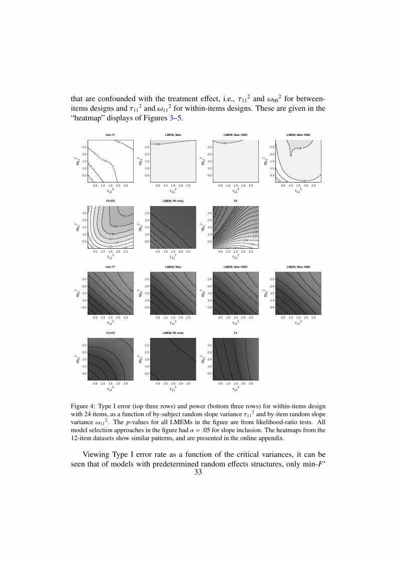
that are confounded with the treatment effect, i.e., τ112 and ω00

2 for between-items designs and τ11

2 and ω112 for within-items designs. These are given in the

“heatmap” displays of Figures 3–5.

min−F'

τ112

ω11

2

0.01

0.02

0.03

0.04

0.5 1.0 1.5 2.0 2.5

0.5

1.0

1.5

2.0

2.5

LMEM, Max

τ112

ω11

2

0.06

0.5 1.0 1.5 2.0 2.5

0.5

1.0

1.5

2.0

2.5

LMEM, Max−NRC

τ112

ω11

2

0.06

0.5 1.0 1.5 2.0 2.5

0.5

1.0

1.5

2.0

2.5

LMEM, Max−NWI

τ112

ω11

2

0.03 0.04 0.05

0.06

0.5 1.0 1.5 2.0 2.5

0.5

1.0

1.5

2.0

2.5

F1+F2

τ112

ω11

2

0.03

0.04

0.0

4

0.04 0.05 0.06

0.07

0.08

0.09

0.1

0.5 1.0 1.5 2.0 2.5

0.5

1.0

1.5

2.0

2.5

LMEM, RI−only

τ112

ω11

2

0.3

0.35 0.4

0.45

0.5

0.5 1.0 1.5 2.0 2.5

0.5

1.0

1.5

2.0

2.5

F1

τ112

ω11

2

0.03 0.04

0.05

0.06

0.07

0.08 0.09

0.1 0.11 0.12 0.13 0.14

0.15 0.

16

0.1

7

0.1

8

0.1

9

0.2

5 0

.3

0.3

5

0.5 1.0 1.5 2.0 2.5

0.5

1.0

1.5

2.0

2.5

min−F'

τ112

ω11

2

0.35

0.4 0.45 0.5

0.6 0.7 0.8

0.9

0.5 1.0 1.5 2.0 2.5

0.5

1.0

1.5

2.0

2.5

LMEM, Max

τ112

ω11

2

0.4

0.45 0.5

0.6

0.7

0.8

0.9

1

0.5 1.0 1.5 2.0 2.5

0.5

1.0

1.5

2.0

2.5

LMEM, Max−NRC

τ112

ω11

2

0.4

0.45

0.5

0.6

0.7

0.8

0.9

1

0.5 1.0 1.5 2.0 2.5

0.5

1.0

1.5

2.0

2.5

LMEM, Max−NWI

τ112

ω11

2

0.4 0.45

0.5 0.6

0.7

0.8

0.9

1

0.5 1.0 1.5 2.0 2.5

0.5

1.0

1.5

2.0

2.5

F1+F2

τ112

ω11

2

0.5

0.6

0.7

0.8

0.9

1

0.5 1.0 1.5 2.0 2.5

0.5

1.0

1.5

2.0

2.5

LMEM, RI−only

τ112

ω11

2

0.9

1

0.5 1.0 1.5 2.0 2.5

0.5

1.0

1.5

2.0

2.5

F1

τ112

ω11

2

0.6

0.7

0.8

0.9 1

0.5 1.0 1.5 2.0 2.5

0.5

1.0

1.5

2.0

2.5

Figure 4: Type I error (top three rows) and power (bottom three rows) for within-items designwith 24 items, as a function of by-subject random slope variance τ11

2 and by-item random slopevariance ω11

2. The p-values for all LMEMs in the figure are from likelihood-ratio tests. Allmodel selection approaches in the figure had α = .05 for slope inclusion. The heatmaps from the12-item datasets show similar patterns, and are presented in the online appendix.

Viewing Type I error rate as a function of the critical variances, it can beseen that of models with predetermined random effects structures, only min-F′

33

maintained the Type I error rate consistently below the α-level throughout theparameter space (Figure 3 and 4). Min-F′ became increasingly conservative asthe relevant random effects got small, replicating Forster & Dickinson (1976).Maximal LMEMs showed no such increasing conservativity, performing welloverall, especially for 24-item datasets. The near-maximal LMEMs also per-formed relatively well, though for within-item datasets, models missing within-unit intercepts became increasingly conservative as slope variances got small.Random-intercepts-only LMEMs degraded extremely rapidly as a function ofrandom slope parameters; even at very low levels of random-slope variability,the Type I error rate was unacceptably high.

In terms of Type I error, the average performance of the widely adoptedF1 × F2 approach is comparable to that of maximal LMEMs (slightly less anti-conservative for 12 items, slightly more anti-conservative for 24 items). But inspite of this apparent good performance, the heatmap visualization indicates thatthe approach is fundamentally unsound. Specifically, F1×F2 shows both conser-vative and anticonservative tendencies: as slopes get small, it becomes increas-ingly conservative, similar to min-F′; as slopes get large, it becomes increasinglyanticonservative, similar to random-intercepts-only LMEMs, though to a lesserdegree. This increasing anticonservativity reflects the fact that (as noted in theintroduction) subject random slopes are not accounted for in the F2 analysis, norare item random slopes accounted for in the F1 analysis (Clark, 1973). The factthat both F1 and F2 analyses have to pass muster keeps this anti-conservativityrelatively minimal as long as subject and/or item slope variances are not large,but the anti-conservativity is there nonetheless.

Figure 5 indicates that despite the overall good performance of some ofthe data-driven approaches, these models become anticonservative when criti-cal variances are small and nonzero.9 This is because as slope variances becomesmall, slopes are less likely to be kept in the model. This anticonservativityvaries considerably with the size of the dataset and the algorithm used (and ofcourse should also vary with the α-level, not depicted in the figure). The anti-conservativity is present to a much stronger degree for the 12-item than for the24-item datasets, reflecting the fact that the critical variances are harder to de-

9Some readers might wonder why the heatmaps for these models show apparent anticonser-vative behavior at the bottom left corner, where the slopes are zero, since performance at thispoint should be close to the nominal level. This is an artifact of the smoothing used in generatingthe heatmaps, which aids in the detection of large trends at the expense of small details. The trueunderlying pattern is that the anticonservativity ramps up extremely quickly from the point wherethe slope variances are zero to reach its maximal value, before beginning to gradually taper away(as the variances become more reliably detected).

34

Backward, Best Path12 items

τ112

ω11

2

0.06

0.07

0.08

0.09 0.1

0.5 1.0 1.5 2.0 2.5

0.5

1.0

1.5

2.0

2.5

Backward, Subjects First12 items

τ112

ω11

2

0.06

0.07

0.08 0.09

0.1

0.5 1.0 1.5 2.0 2.5

0.5

1.0

1.5

2.0

2.5

Backward, Items First12 items

τ112

ω11

2

0.06

0.07 0.08

0.09

0.1

0.5 1.0 1.5 2.0 2.5

0.5

1.0

1.5

2.0

2.5

Forward, Best Path12 items

τ112

ω11

2

0.06

0.07

0.08

0.09 0.1

0.5 1.0 1.5 2.0 2.5

0.5

1.0

1.5

2.0

2.5

Forward, Subjects First12 items

τ112

ω11

2

0.05

0.06

0.06

0.07 0.0

7 0.0

8 0

.09

0.1

0.1

1 0

.12

0.1

3

0.14

0.1

5 0

.16

0.1

7 0

.18

0.1

9

0.2

0

.25

0.3

0

.35

0.4

0

.45

0.5

0.5 1.0 1.5 2.0 2.5

0.5

1.0

1.5

2.0

2.5

Forward, Items First12 items

τ112

ω11

2

0.07

0.07

0.08

0.09 0.1 0.11

0.12

0.13 0.14

0.15

0.16

0.17

0.18

0.19 0.2

0.25

0.3

0.35

0.5 1.0 1.5 2.0 2.5

0.5

1.0

1.5

2.0

2.5

Backward, Best Path24 items

τ112

ω11

2

0.06

0.06

0.07

0.08

0.5 1.0 1.5 2.0 2.5

0.5

1.0

1.5

2.0

2.5

Backward, Subjects First24 items

τ112

ω11

2

0.06

0.06

0.07

0.5 1.0 1.5 2.0 2.5

0.5

1.0

1.5

2.0

2.5

Backward, Items First24 items

τ112

ω11

2

0.06

0.06

0.07

0.5 1.0 1.5 2.0 2.5

0.5

1.0

1.5

2.0

2.5

Forward, Best Path24 items

τ112

ω11

2

0.06

0.06

0.07

0.08

0.5 1.0 1.5 2.0 2.5

0.5

1.0

1.5

2.0

2.5

Forward, Subjects First24 items

τ112

ω11

2 0.04

0.04

0.0

5

0.05

0.0

6

0.06

0.0

7

0.0

8

0.0

9

0.1

0

.11

0.1

2 0

.13

0.1

4 0

.15

0.1

6

0.1

7

0.1

8

0.1

9

0.2

0

.25

0.3

0

.35

0.4

0.5 1.0 1.5 2.0 2.50.

51.

01.

52.

02.

5

Forward, Items First24 items

τ112

ω11

2

0.04

0.04

0.05

0.05

0.06

0.06

0.07 0.08 0.09

0.1 0.11 0.12

0.13

0.14 0.15

0.16

0.17 0.18

0.19

0.2

0.25

0.3 0.35

0.4

0.5 1.0 1.5 2.0 2.5

0.5

1.0

1.5

2.0

2.5

Backward, Best Path12 items

τ112

ω11

2

0.3

0.35

0.4

0.45 0.5

0.6

0.7

0.8

0.9 1

0.5 1.0 1.5 2.0 2.5

0.5

1.0

1.5

2.0

2.5

Backward, Subjects First12 items

τ112

ω11

2

0.3

0.35

0.4

0.45 0.5

0.6

0.7

0.8

0.9 1

0.5 1.0 1.5 2.0 2.5

0.5

1.0

1.5

2.0

2.5

Backward, Items First12 items

τ112

ω11

2

0.3

0.35

0.4

0.45 0.5

0.6

0.7 0.8

0.9 1

0.5 1.0 1.5 2.0 2.5

0.5

1.0

1.5

2.0

2.5

Forward, Best Path12 items

τ112

ω11

2

0.3

0.35

0.4

0.45

0.5

0.6

0.7

0.8

0.9 1

0.5 1.0 1.5 2.0 2.5

0.5

1.0

1.5

2.0

2.5

Forward, Subjects First12 items

τ112

ω11

2

0.3

0.35

0.4

0.45 0.5

0.6 0.7

0.8 0.9

1

0.5 1.0 1.5 2.0 2.5

0.5

1.0

1.5

2.0

2.5

Forward, Items First12 items

τ112

ω11

2

0.3

0.35

0.4

0.45 0.5

0.6

0.7

0.8

0.9 1 0.5 1.0 1.5 2.0 2.5

0.5

1.0

1.5

2.0

2.5

Backward, Best Path24 items

τ112

ω11

2

0.4

0.45

0.5

0.6

0.7

0.8

0.9

1

0.5 1.0 1.5 2.0 2.5

0.5

1.0

1.5

2.0

2.5

Backward, Subjects First24 items

τ112

ω11

2

0.4

0.45

0.5

0.6

0.7

0.8

0.9

1

0.5 1.0 1.5 2.0 2.5

0.5

1.0

1.5

2.0

2.5

Backward, Items First24 items

τ112

ω11

2

0.4

0.45

0.5

0.6

0.7

0.8

0.9

1

0.5 1.0 1.5 2.0 2.5

0.5

1.0

1.5

2.0

2.5

Forward, Best Path24 items

τ112

ω11

2

0.4

0.45

0.5

0.6

0.7

0.8

0.9

1

0.5 1.0 1.5 2.0 2.5

0.5

1.0

1.5

2.0

2.5

Forward, Subjects First24 items

τ112

ω11

2

0.4 0.45

0.5

0.6 0.7 0.8

0.9

1

0.5 1.0 1.5 2.0 2.5

0.5

1.0

1.5

2.0

2.5

Forward, Items First24 items

τ112

ω11

2

0.4

0.45

0.5

0.6

0.7

0.8

0.9 1 0.5 1.0 1.5 2.0 2.5

0.5

1.0

1.5

2.0

2.5

Figure 5: Type I error (top two rows) and power (bottom two rows) for design-driven approacheson within-items data, as a function of by-subject random slope variance τ11

2 and by-item randomslope variance ω11

2. The p-values for all LMEMs in the figure are from likelihood-ratio tests.All approaches in the figure tested random slopes at α = .05.

35

tect with smaller data sets. The forward stepping models that tested slopes in anarbitrary sequence were the most anticonservative by far. The model testing theby-subject slope first performed most poorly when that slope variance was smalland the by-item slope variance was large, because in such cases the algorithmwould be likely to stop at a random-intercepts-only model, and thus would nevertest for the inclusion of the by-item slope. By the same principles, the forwardmodel that tested the by-item slope first showed worst performance when theby-item slope variance was small and the by-subject slope variance large.

In sum, insofar as one is concerned about drawing conclusions likely to gen-eralize across subjects and items, only min-F′ and maximal LMEMs can be saidto be fundamentally sound across the full parameter space that we surveyed. F1-only and random-intercepts-only LMEMs are fundamentally flawed, as are for-ward stepping models that follow an arbitrary sequence, especially in cases withfew observations. All other LMEMs with model selection showed small amountsof anticonservativity when slopes were small, even when the slopes were testedin a principled sequence; however, this level of anticonservativity is probably tol-erable for reasonably-sized datasets (so long as there is not an extensive amountof missing data; see online appendix). The widely-used F1 × F2 approach isflawed as well, but may be acceptable in cases where maximal LMEMs are notapplicable. The question now is which of these analyses best maximizes power(Tables 5 and 6; Figures 3 and 4).

Overall, maximal LMEMs showed greater power than min-F′. When cor-rected for their slight anticonservativity, maximal LMEMs exhibited power thatwas between 4% and 6% higher for the between-items design than the uncor-rected values for min-F′. Although there does not seem to be a large overallpower advantage to using maximal LMEMs for between-item designs, the vi-sualization of power in terms of the critical variances (Figure 3) suggests thatthe power advantage increases slightly as the critical variances become small. Incontrast, maximal LMEMs showed a considerable power advantage for within-item designs, with corrected power levels for α=.05 (.433 and .592) that were16% to 32% higher than the uncorrected power values for min-F′ (.327 and.512). This additional power of maximal LMEMs cannot be attributed to the in-clusion of cases where slopes were removed due to nonconvergence, since in theworst case (the within-item dataset with 12 items) virtually all simulation runs(99.613%) converged with the maximal structure.

Note that the corrected power for random-intercepts-only LMEMs was actu-ally below that of maximal LMEMs (between-items: .216 and .314 for 12 and24 items respectively; within-items: .380 and .531). This means that most of the

36

apparent additional power of maximal LMEMs over min-F′ is real, while mostof the apparent power of random-intercepts-only LMEMs is, in fact, illusory.

Our results show that it is possible to use a data-driven approach to specifyingrandom effects in a way that minimizes Type I error, especially with “best-path”model selection. However, the power advantage of this approach for continuousdata, even when uncorrected for anticonservativity, is very small. In short, data-driven approaches can produce reasonable results, but their very small benefit topower may not be worth the additional uncertainty they introduce as comparedto a design-driven approach.

0.0

0.2

0.4

0.6

0.8

1.0

pow

er

Between Item, N=12

(.00

0, .0

42]

(.04

2, .0

84]

(.08

4, .1

26]

(.12

6, .1

68]

(.16

8, .2

11]

(.21

1, .2

53]

(.25

3, .2

95]

(.29

5, .3

37]

(.33

7, .3

79]

(.37

9, .4

21]

(.42

1, .4

63]

(.46

3, .5

05]

(.50

5, .5

47]

(.54

7, .5

89]

(.58

9, .6

32]

(.63

2, .6

74]

(.67

4, .7

16]

(.71

6, .7

58]

(.75

8, .8

00]

MaximalRandom Interceptmin−F'F1xF2

effect

0.0

0.2

0.4

0.6

0.8

1.0

pow

er

Between Item, N=24

(.00

0, .0

42]

(.04

2, .0

84]

(.08

4, .1

26]

(.12

6, .1

68]

(.16

8, .2

11]

(.21

1, .2

53]

(.25

3, .2

95]

(.29

5, .3

37]

(.33

7, .3

79]

(.37

9, .4

21]

(.42

1, .4

63]

(.46

3, .5

05]

(.50

5, .5

47]

(.54

7, .5

89]

(.58

9, .6

32]

(.63

2, .6

74]

(.67

4, .7

16]

(.71

6, .7

58]

(.75

8, .8

00]

MaximalRandom Interceptmin−F'F1xF2

effect

0.0

0.2

0.4

0.6

0.8

1.0po

wer

Within Item, N=12

(.00

0, .0

42]

(.04

2, .0

84]

(.08

4, .1

26]

(.12

6, .1

68]

(.16

8, .2

11]

(.21

1, .2

53]

(.25

3, .2

95]

(.29

5, .3

37]

(.33

7, .3

79]

(.37

9, .4

21]

(.42

1, .4

63]

(.46

3, .5

05]

(.50

5, .5

47]

(.54

7, .5

89]

(.58

9, .6

32]

(.63

2, .6

74]

(.67

4, .7

16]

(.71

6, .7

58]

(.75

8, .8

00]

MaximalRandom Interceptmin−F'F1xF2

effect

0.0

0.2

0.4

0.6

0.8

1.0

pow

er

Within Item, N=24

(.00

0, .0

42]

(.04

2, .0

84]

(.08

4, .1

26]

(.12

6, .1

68]

(.16

8, .2

11]

(.21

1, .2

53]

(.25

3, .2

95]

(.29

5, .3

37]

(.33

7, .3

79]

(.37

9, .4

21]

(.42

1, .4

63]

(.46

3, .5

05]

(.50

5, .5

47]

(.54

7, .5

89]

(.58

9, .6

32]

(.63

2, .6

74]

(.67

4, .7

16]

(.71

6, .7

58]

(.75

8, .8

00]

MaximalRandom Interceptmin−F'F1xF2

effect

Figure 6: Statistical power for maximal LMEMs, random-intercepts-only LMEMs, min-F′, andF1 × F2 as a function of effect size, when the generative model underlying the data is a random-intercepts-only LMEM.

The above analyses suggest that maximal LMEMs are in no way conserva-tive, at least for the analysis of continuous data. To dispel this suspicion en-tirely it is illustrative to consider the performance of maximal LMEMs in anextreme case for which their power should be at its absolute worst: namely,when the random slope variance is negligible, such that the underlying processis best described by a random-intercepts-only LMEM. Comparing the perfor-mance of maximal LMEMs to random-intercepts-only LMEMs in this circum-stance can illustrate the highest “cost” that one could possibly incur by usingmaximal LMEMs in the analysis of continuous data. Maximal LMEMs mightperform badly in this situation because they overfit the underlying generativeprocess, loosely akin to assuming too few degrees of freedom for the analysisrather than too many. But they might also perform tolerably well to the extentthat the estimation procedure for LMEMs can detect that a random effect param-eter is effectively zero. In this situation, it is additionally informative to comparethe power of maximal LMEMs not only to random-intercepts-only LMEMs, butalso to that of min-F′, since min-F′ is generally regarded as conservative, aswell as to that of F1 × F2, since F1 × F2 is generally regarded as sufficiently

37

powerful. If maximal LMEMs perform better than min-F′ and at least as well asF1 × F2, then that would strongly argue against the idea that maximal LMEMsare unduly conservative. To address this, we conducted an additional set of sim-ulations, once again using the data-generating parameters in Table 2, except thatwe set all random-slope variances to 0, so that the model generating the datawas a random-intercepts-only LMEM; also, we varied the true fixed effect sizecontinuously from 0 to 0.8.

The results were unambiguous (Figure 6): even in this worst case scenariofor their power, maximal LMEMs consistently showed higher power than min-F′ and even F1 × F2; indeed, for within-items designs, they far outstripped theperformance of F1 × F2, an approach whose power is rarely questioned. Forbetween-items designs, maximal LMEMs incurred a negligible cost relative torandom-intercepts-only LMEMs, while for within-items designs, there was onlya minor cost that diminished as the number of items increased. Overall, thecost/benefit analysis favors maximal LMEMs over other approaches. Note thatover the four different sets of simulations in Figure 6, our maximal LMEM anal-ysis procedure stepped down to a random-intercept model (due to convergenceproblems) on less than 3% of runs. Thus, these results indicate good performanceof the estimation algorithm when random slope variances are zero.

The case of within-item designs with few items showed the biggest differencein power between random-intercepts-only models and maximal LMEMs. Thesize of this difference indicates the maximum benefit that could be obtained, inprinciple, by using a data-driven approach. However, in practice, the ability of adata-driven approach to detect random slope variation diminishes as the datasetgets small. In other words, it is in just this situation that the power for detectingrandom slope variation is at its worst (see Figure 4 and the 12-item figures in theAppendix); thus, in this case, the payoff in terms of statistical power over themaximal approach does not outweigh the additional risk of anticonservativity.

In sum, our investigation suggests that for confirmatory hypothesis testing,maximal LMEMs yield nearly optimal performance: they were better than allother approaches except min-F′ at maintaining the Type I error rate near thenominal level. Furthermore, unlike F1 × F2 and certain model selection ap-proaches, maximal LMEMs held the error rate relatively close to nominal acrossthe entirety of the parameter space. And once corrected for anticonservativity,no other technique exceeded the power of maximal LMEMs. “best-path” modelselection also kept Type I errors largely at bay, but it is not clear whether theylead to gains in statistical power.

The near-optimal performance of maximal models may be explained as fol-

38

lows. Including the random variances that could potentially be confounded withthe effect of interest is critical to controlling the Type I error rate, by ensuring thatthe assumption of conditional independence is met. Including random variancesthat are not confounded with that effect (e.g., within-unit intercept variances) isnot critical for reducing Type I error, but nonetheless reduces noise and thus in-creases the sensitivity of the test. Including only those random components thatreduce noise but not those that are confounded with the effect of interest willlead to drastically anticonservative behavior, as seen by random-intercepts-onlyLMEMs, which had the worst Type I error rates overall.

General Discussion

Recent years have witnessed a surge in the popularity of LMEMs in psy-cholinguistics and related fields, and this growing excitement is well deserved,given the great flexibility of LMEMs and their ability to model the generativeprocess underlying one’s data. However, there has been insufficient apprecia-tion of how choices about random effect structure impact generalizability, andno accepted standards for the use of LMEMs in confirmatory hypothesis testingare currently in place. We have emphasized that specifying random effects inLMEMs involves essentially the same principles as selecting an analysis tech-nique from the menu of traditional ANOVA-based options. The standard forANOVA has been to assume that if an effect exists, subjects and/or items willvary in the extent to which they show that effect. This is evident in the fact thatresearchers using ANOVA have tended to assume the maximal (or near-maximal)random effects structure justified by the design.

Our survey of various analysis strategies for confirmatory hypothesis testingon data with crossed random effects clearly demonstrates that the strongest con-tenders in avoiding anti-conservativity are maximal LMEMs and min-F′ (seebelow for related discussion of data-driven approaches). These were the onlyapproaches that consistently showed nominal or near-nominal Type I error ratesthroughout the parameter space. Although maximal LMEMs showed some mi-nor anticonservativity, our analysis has uncovered a hidden advantage of max-imal LMEMs over ANOVA-based approaches. This advantage was evident inthe diverging performance of these approaches as a function of the critical vari-ances (the variances confounded with the effect of interest). As these variancesbecame small, maximal LMEMs showed better retention of their power relativeto ANOVA-based approaches, which became increasingly conservative. In thelimit, when the generative process did not include any random slope variation,the power of maximal LMEMs substantially outstripped that of ANOVA-based

39

approaches, even F1 × F2. An apparent reason for this power advantage of max-imal LMEMs is their simultaneous accommodation of by-subject and by-itemrandom variation. ANOVA-based approaches are based on two separately cal-culated statistics, one for subjects and one for items, each of which does not con-trol for the variance due to the other random factor. Specifically, the prominentdecrease in power for ANOVA-based approaches when critical random variancesare small could be due to the fact that separate F1 × F2 analyses cannot distin-guish between random intercept variation on the one hand and residual noise onthe other: by-item random intercept variation is conflated with trial-level noisein the F1 analysis, and by-subject random intercept variation is conflated withtrial-level noise in the F2 analysis. Maximal LMEMs do not suffer from thisproblem.

The performance of LMEMs depended strongly on assumptions about ran-dom effects. This clearly implies that researchers who wish to use LMEMs needto be more attentive both to how they specify random effects in their models, andto the reporting of their modeling efforts. Throughout this article, we have arguedthat for confirmatory analyses, a design-driven approach is preferable to a data-driven approach for specifying random effects. By using a maximal model, oneadheres to the longstanding (and eminently reasonable) assumption that if an ef-fect exists, subjects and/or items will most likely vary in the extent to which theyshow that effect, whether or not that variation is actually detectable in the sam-ple. That being said, it seems likely that effect variation across subjects and/oritems differs among research areas. Perhaps there are even effects for which suchvariation is effectively negligible. In such cases, one might argue that a maximalLMEM is “overfitting” the data, which is detrimental to power. However, oursimulations (Figure 6) show that maximal LMEMs would not be unreasonablyconservative in such cases, at least for continuous data; indeed, they are far morepowerful than even F1 × F2.

Many researchers have used a data-driven approach to determining the ran-dom effects structure associated with confirmatory analysis of a fixed effect ofparticular interest.10 Our simulations indicate that it is possible to obtain reason-able results with such an approach, if generous criteria for the inclusion of ran-dom effects are used. However, it is important to bear in mind that data-driven

10We note here that arguments for data-driven effects to random-effects structure have beenmade within the ANOVA literature as well (e.g., Raaijmakers et al., 1999), and that these argu-ments have not won general acceptance within the general psycholinguistics community. Fur-thermore, part of the appeal of those arguments was the undue conservativity of min-F′; sincemaximal LMEMs do not suffer from this problem, we take the arguments for data-driven random-effects specification with them to be correspondingly weaker.

40

approaches always imply some sort of tradeoff between Type-I and Type-II errorprobability, and that it is difficult to precisely quantify the tradeoff that one hastaken. It is partly for this reason that the use of data-driven approaches is con-troversial, even among statistical experts (Bolker et al., 2009; see also Harrell,2001 for more general concerns regarding model selection). Our results showthat data-driven approaches yield varying performance in terms of Type I errordepending on the criteria and algorithm used, the size of the dataset, the ex-tent of missing data, and the design of the study (which determines the numberof random effect terms that need to be tested). It may be difficult for a readerlacking access to the original data to to quantify the resulting Type I/II errortradeoff, even when the inclusion criteria are known. Still, there are situations inwhich data-driven approaches may be justifiable, such as when the aims are notfully confirmatory, or when one experiences severe convergence problems (seebelow).

Overall, our analysis suggests that, when specifying random effects for hy-pothesis testing with LMEMs, researchers have been far too concerned aboutoverfitting the data, and not concerned enough about underfitting the design. Infact, it turns out overfitting the data with a maximal model has only minimal con-sequences for Type I error and power—at least for the simple designs for typicalpsycholinguistic datasets considered here—whereas underfitting the design canincur levels of anticonservativity ranging anywhere from minor (best-path modelselection) to extremely severe (random-intercepts-only LMEMs) with little realbenefit to power. In the extreme, random-intercepts-only models have the worstgeneralization performance of any approach to date when applied to continuousdata with within-subjects and within-item manipulations. This goes to show that,for such designs, crossing of random by-subject and by-item intercepts alone isclearly not enough to ensure proper generalization of experimental treatmenteffects (a misconception that is unfortunately rather common at present). In psy-cholinguistics, there are few circumstances in which we can know a priori that arandom-intercepts-only model is truly justified (see further below). Of course, ifone wishes to emphasize the absence of evidence for a given effect, there couldbe some value in demonstrating that the effect is statistically insignificant evenwhen a random-intercepts-only model is applied.

Our general argument applies in principle to the analysis of non-normallydistributed data (e.g., categorical or count data) because observational depen-dencies are mostly determined by the design of an experiment and not by theparticular type of data being analyzed. However, practical experience with fit-ting LMEMs to datasets with categorical response variables, in particular with

41

mixed logit models, suggests more difficulty in getting maximal models to con-verge. There are at least three reasons for this. First, the estimation algorithmsfor categorical responses differ from the more developed procedures in estimat-ing continuous data. Second, observations on a categorical scale (e.g., whether aresponse is accurate or inaccurate) typically carry less information about param-eters of interest than observations on a continuous scale (e.g., response time).Third, parameter estimation for any logistic model is challenging when the un-derlying probabilities are close to the boundaries (zero or one), since the inverselogit function is rather flat in this region. So although our arguments and recom-mendations (given below) still apply in principle, they might need to be modifiedfor noncontinuous cases. For example, whereas we observed for continuous datathat cases in which the random effect structure “overfit” the data had minimal im-pact on performance, this might not be the case for categorical data, and perhapsdata-driven strategies would be more justifiable. In short, although we maintainthat design-driven principles should govern confirmatory hypothesis testing onany kind of data, we acknowledge that there is a pressing need to evaluate howthese principles can be best applied to categorical data.

In our investigation we have only looked at a very simple one-factor designwith two levels. However, we see no reason why our results would not gen-eralize to more complex designs. The principles are the same in higher-orderdesigns as they are for simple one-factor designs: any main effect or interactionfor which there are multiple observations per subject or item can vary acrossthese units, and, if this dependency is not taken into account, the p-values willbe biased against the null hypothesis.11 The main difference is that models withmaximal random effects structure would be less likely to converge as the num-ber of within-unit manipulations increases. In the next section, we offer someguidelines for how to cope with nonconverging models.

Producing generalizable results with LMEMs: Best practicesOur theoretical analyses and simulations lead us to the following set of rec-

ommended “best practices” for the use of LMEMs in confirmatory hypothesistesting. It is important to be clear that our recommendations may not apply tosituations where the overarching goal is not fully confirmatory. Furthermore,

11To demonstrate this, we conducted Monte Carlo simulation of a 24-subject, 24-item 2×2within/within experiment with main fixed effects, no fixed interaction, and random by-subjectand by-item interactions. When analyzed with random-intercepts-only LMEMs, we found aType I error rate of .69; with maximal LMEMs the Type I error rate was .06. A complete reportof these simulations appears in the supplementary appendix.

42

we offer these not as the best possible practices—as our understanding of thesemodels is still evolving—but as the best given our current level of understanding.

Identifying the maximal random effects structureBecause the same principles apply for specifying subject and item random ef-

fects, to simplify the exposition in this section we will only talk about “by-unit”random effects, where “unit” stands in for the sampling unit under considera-tion (subjects or items). As we have emphasized throughout this paper, the sameconsiderations come into play when specifying random effects as when choos-ing from the menu of traditional analyses. So the first question to ask oneselfwhen trying to specify a maximal LMEM is: which factors are within-unit, andwhich are between? If a factor is between-unit, then a random intercept is usuallysufficient. If a factor is within-unit and there are multiple observations per treat-ment level per unit, then you need a by-unit random slope for that factor. Theonly exception to this rule is when you only have a single observation for everytreatment level of every unit; in this case, the random slope variance would becompletely confounded with trial-level error. It follows that a model with a ran-dom slope would be unidentifiable, and so a random intercept would be sufficientto meet the conditional independence assumption. For datasets that are unbal-anced across the levels of a within-unit factor, such that some units have veryfew observations or even none at all at certain levels of the factor, one should atleast try to estimate a random slope (but see the caveats below about how sucha situation may contribute to nonconvergence). Finally, in cases where there isonly a single observation for every unit, of course, not even a random intercept isneeded (one can just use ordinary regression as implemented in the R functionslm() and glm()).

The same principles apply to higher-order designs involving interactions. Inmost cases, one should also have by-unit random slopes for any interactionswhere all factors comprising the interaction are within-unit; if any one factorinvolved in the interaction is between-unit, then the random slope associatedwith that interaction cannot be estimated, and is not needed. The exception tothis rule, again, is when you have only one observation for every subject in everycell (i.e., unique combination of factor levels). If some of the cells for someof your subjects have only one or zero observations, you should still try to fit arandom slope.

Random effects for control predictorsOne of the most compelling aspects of mixed-effects models is the ability to

include almost any control predictor—by which we mean a property of an exper-43

imental trial which may affect the response variable but is not of theoretical inter-est in a given analysis—desired by the researcher. In principle, including controlvariables in an analysis can rule out potential confounds and increase statisticalpower by reducing residual noise. Given the investigations in the present paper,however, the question naturally arises: in order to guard against anti-conservativeinference about a predictor X of theoretical interest, do we need by-subject andby-item random effects for all our control predictors C as well? Suppose, afterall, if there is no underlying fixed effect of C but there is a random effect ofC—could this create anti-conservative inference in the same way as omitting arandom effect of X in the analysis could? To put this issue in perspective viaan example, Kuperman et al. (2010) include a total of eight main effects in anLME analysis of fixation durations in Dutch reading; for the interpretation ofeach main effect, the other seven may be thought of as serving as controls. Fit-ting eight random effects, plus correlation terms, would require estimating 72random effects parameters, 36 by-subject and 36 by item. One would likely needa huge dataset to be able to estimate all the effects reliably (and one must alsonot be in any hurry to publish, for even with huge amounts of data such modelscan take extremely long to converge).

To our knowledge, there is little guidance on this issue in the existing lit-erature, and more thorough research is needed. Based on a limited amount ofinformal simulation, however (reported in the online Appendix), we propose theworking assumption that it is not essential for one to specify random effects forcontrol predictors to avoid anticonservative inference, as long as interactions be-tween the control predictors and the the factors of interest are not present in themodel (or justified by the data). Once again, we emphasize the need for futureresearch on this important issue.

Coping with failures to convergeIt is altogether possible and unfortunately common that the estimation pro-

cedure for LMEMs will not converge with the full random-effects specification.In our experience, the likelihood that a model will converge depends on two fac-tors: (1) the extent to which random effects in the model are large, and (2) theextent to which there are sufficient observations to estimate the random effects.Generally, as the sizes of the subject and item samples grow, the likelihood ofconvergence will increase. Of course, one does not always have the luxury ofusing many subjects and items. And, although the issue seems not to have beenstudied systematically, it is our impression that fitting maximal LMEMs is lessoften successful for categorical data than for continuous data.

It is important, however, to resist the temptation to step back to random-44

intercepts-only models purely on the grounds that the maximal model does notconverge. When the maximal LMEM does not converge, the first step shouldbe to check for possible misspecifications or data problems that might accountfor the error. It may also help to use standard outlier removal methods and tocenter or sum-code the predictors. In addition, it may sometimes be effective toincrease the maximum number of iterations in the estimation procedure.

Once data and model specification problems have been eliminated, the nextstep is to ask what simplification of one’s model’s random-effects structure is themost defensible given the goals of one’s analysis. In the common case whereone is interested in a minimally anti-conservative evaluation of the strength ofevidence for the presence of an effect, our results indicate that keeping the ran-dom slope for the predictor of theoretical interest is important: a maximal modelwith no random correlations or even missing within-unit random intercepts ispreferable to one missing the critical random slopes. Our simulations suggestthat removing random correlations might be a good strategy, as this model per-formed similarly to maximal LMEMs.12

However, when considering this simplification strategy, it is important to firstcheck whether the nonconvergence might be attributable to the presence of a fewsubjects (or items) with small numbers of observations in particular cells. If thisis the case, it might be preferable to remove (or replace) these few subjects (oritems) rather than to remove an important random slope from the model. For ex-ample, Jaeger et al. (2011, section 3.3) discuss a case involving categorical datain which strong evidence for random slope variation was present when subjectswith few observations were excluded, but not when they were kept in the dataset.

For more complex designs, of course, the number of possible random-effectsstructures proliferate. Research is needed to evaluate the various possible strate-gies that one could follow when one cannot fit a maximal model. Both ourtheoretical analysis and simulations suggest a general rule of thumb: for what-ever fixed effects are of critical interest, the corresponding random effects shouldbe present in that analysis. For a study with multiple fixed effects of theoret-ical interest, and for which a model including random effects for all these keyeffects does not converge, separate analyses can be pursued. For example, in astudy where confirmatory analysis of fixed effects for X1 and X2 is desired, twoseparate analyses may be in order—one with (at least) random slopes for X1 to

12We remind the reader that the no-correlation and RS-only models are sensitive to the codingused for the predictor; our theoretical analysis and simulation results indicate that deviationcoding is generally preferable to treatment coding; see online Appendix.

45

test the evidence for generalization of X1, and another with (at least) randomslopes for X2 to test X2. (One would typically still want to include the fixedeffects for X1 and X2 in both models, of course, for the established reason thatmultiple regression reveals more information than two separate regressions withsingle predictors; and see also the previous section on random effects for controlpredictors.)

One fallback strategy for coping with severe convergence problems is to use adata-driven approach, building up in a principled way from a very simple model(e.g., a model with all fixed effects but only a single by-subjects random inter-cept, or even no random effects at all). Our simulations indicate that it is possibleto use forward model selection in a way that guards against anticonservativity if,at each step, one tests for potential inclusion all random effects not currently inthe model, and include any that pass at a relatively liberal α-level (e.g., .20; seeMethod section for further details about the “best path” algorithm). We warnthe reader that, with more complex designs, the space of possible random-effectsspecifications is far richer than typically appreciated, and it is easy to design amodel-selection procedure that fails to get to the best model. As just one ex-ample, in a “within” 2 × 2 design with factors A and B, it is possible to havea model with a random interaction term but no random main-effect slopes. Ifone is interested in the fixed-effect interaction but only tests for a random inter-action if both main-effect random slopes are already in the model, then if thetrue generative process underlying the data has a large random interaction butnegligible random main-effect slopes then forward model selection will be badlyanti-conservative. Thus it is critical to report the modeling strategy in detail sothat it can be properly evaluated.

A final recommendation is based on the fact that maximal LMEMs will bemore likely to converge when the random effects are large, which is exactlythe situation where F1 × F2 is anti-conservative. This points toward a possiblepractice of trying to fit a maximal LMEM wherever possible, and when it is not,to drop the concept of crossed random effects altogether and perform separate by-subject and by-item LMEMs, similar in logic to F1 × F2, each with appropriatemaximal random effect structures. In closing, it remains unresolved which ofthese strategies for dealing with nonconvergence is ultimately most beneficial,and we hope that future studies will investigate their impact on generalizabilitymore systematically.

Computing p-valuesThere are a number of ways to compute p-values from LMEMs, none of

which is uncontroversially the best. Although Baayen et al. (2008) recommended46

using Monte Carlo Markov Chain (MCMC) simulation, this is not yet possible inlme4 for models with correlation parameters, and our simulations indicate thatthis method for obtaining p-values is more anticonservative than the other twomethods we examined (at least using the current implementation and defaultsfor MCMC sampling in lme4 and languageR).13 Also, it is important to notethat MCMC sampling does nothing to mitigate the anticonservativity of random-intercept-only LMEMs when random slope variation is present.

For obtaining p-values from analyses of typically-sized psycholinguisticdatasets—where the number of observations usually far outnumbers the num-ber of model parameters—our simulations suggest that the likelihood-ratio testis the best approach. To perform such a test, one compares a model contain-ing the fixed effect of interest to a model that is identical in all respects exceptthe fixed effect in question. One should not also remove any random effectsassociated with the fixed effect when making the comparison. In other words,likelihood-ratio tests of a fixed effect with k levels should have only k − 1 de-grees of freedom (e.g., one degree of freedom for the dichotomous single-factorstudies in our simulations). We have seen cases where removing the fixed effectcauses the comparison model to fail to converge. Under these circumstances, onemight alter the comparison model following the procedures described above toattempt to get it to converge, and once convergence is achieved, compare it to anidentical model including the fixed effect. Note that our results indicate that theconcern voiced by Pinheiro & Bates (2000) regarding the anti-conservativity oflikelihood-ratio tests to assess fixed effects in LMEMs is probably not applicableto datasets of the typical size of a psycholinguistic study (see also Baayen et al.,2008, footnote 1).

Reporting resultsIt is not only important for researchers to understand the importance of using

maximal LMEMs, but also for them to articulate their modeling efforts with suf-ficient detail so that other researchers can understand and replicate the analysis.In our informal survey of papers published in JML, we sometimes found nothingmore than a mere statement that researchers used “a mixed effects model withrandom effects for subjects and items.” This could be anything from a random-intercepts-only to a maximal LMEM, and obviously, there is not enough infor-mation given to assess the generalizability of the results. One needs to provide

13MCMC simulations for random-slopes and more complex mixed-effects models can be runwith general-purpose graphical models software such as WinBUGS (Lunn et al., 2000), JAGS(Plummer, 2003), or MCMCglmm (Hadfield, 2010). This approach can be delicate and error-prone, however, and we do not recommend it at this point as a general practice for the field.

47

sufficient information for the reader to be able to recreate the analyses. One wayof satisfying this requirement is to report the variance-covariance matrix, whichincludes all the information about the random effects, including their estimates.This is useful not only as a check on the random effects structure, but also forfuture meta-analyses. A simpler option is to mention that one attempted to usea maximal LMEM and, as an added check, also state which factors had randomslopes associated with them. If the random effects structure had to be simplifiedto obtain convergence, this should also be reported, and the simplifications thatwere made should be justified to the extent possible.

If it is seen as necessary or desireable in a confirmatory analysis to deter-mine the random effects structure using a data-driven approach, certain minimalguidelines should be followed. First, it is critical to report the criteria that havebeen used, including the α-level for exclusion/inclusion of random slopes andthe order in which random slopes were tested. Furthermore, authors should ex-plicitly report the changed assumptions about the generative process underlyingthe data that result from excluding the random slope (rather than just statingthat the slopes did not “improve model fit”), and should do so in non-technicallanguage that non-experts can understand. Readers with only background inANOVA will not understand that removing the random slope corresponds topooling error across strata in a mixed-model ANOVA analysis. It is thereforepreferable to clearly state the underlying assumption of a constant effect, e.g.,“by excluding the random slope for the priming manipulation, we assume thatthe priming effect is invariant across subjects (or items) in the population.”

Concluding remarksIn this paper we have focused largely on confirmatory analyses. We hope

this emphasis will not be construed as an endorsement of confirmatory over ex-ploratory approaches. Exploratory analysis is an important part of the cycle ofresearch, without which there would be few ideas to confirm in the first place.We do not wish to discourage people from exploiting all the many new and ex-citing opportunities for data analysis that LMEMs offer (see Baayen, 2008 foran excellent overview). Indeed, one of the situations in which the exploratorypower of LMEMs can be especially valuable is in performing a “post-mortem”analysis on confirmatory studies that yield null or ambiguous results. In suchcircumstances, one should pay careful attention to the estimated random effectscovariance matrices from the fitted model, as they provide a map of one’s igno-rance. For instance, when a predicted fixed effect fails to reach significance, itis informative to check whether subjects or items have larger random slopes for

48

that effect, and to then use whatever additional data one has on hand (e.g., demo-graphic information) to try to reduce this variability. Such investigation can beextremely useful in planning further studies (or in deciding whether to cut one’slosses), though of course such findings should be interpreted with caution, andtheir post-hoc nature should be honestly reported (Wagenmakers et al., in press).

At a recent workshop on mixed-effects models, a prominent psycholinguist14

memorably quipped that encouraging psycholinguists to use linear mixed-effectsmodels was like giving shotguns to toddlers. Might the field be better off withoutcomplicated mixed-effects modeling, and the potential for misuse it brings? Al-though we acknowledge this complexity and its attendant problems, we feel thatone of the reasons why researchers have been using mixed-effects models inap-propriately in confirmatory analyses is due to the misconception that they aresomething entirely new, a misconception that has prevented seeing the continuedapplicability of their previous knowledge about what a generalizable hypothesistest requires. As we hope to have shown, by and large, researchers already knowmost of what is needed to use LMEMs appropriately. So long as we can continueto adhere to the standards that are already implicit, we therefore should not denyourselves access to this new addition to the statistical arsenal. After all, when ourinvestigations involve stalking a complex and elusive beast (whether the humanmind or the feline palate), we need the most powerful weapons at our disposal.

Acknowledgements

We thank Ian Abramson, Harald Baayen, Klinton Bicknell, Ken Forster, Si-mon Garrod, Philip Hofmeister, Florian Jaeger, Keith Rayner, and NathanielSmith for helpful discussion, feedback, and suggestions. This work has been pre-sented at seminars and workshops in Bielefeld, Edinburgh, York, and San Diego.A supplementary appendix is available online (http://talklab.psy.gla.ac.uk/simgen).

References

Baayen, R. H. (2004). Statistics in psycholinguistics: A critique of some current gold standards.Mental Lexicon Working Papers, 1, 1–45.

Baayen, R. H. (2008). Analyzing linguistic data: A practical introduction to statistics using R.Cambridge: Cambridge University Press.

Baayen, R. H. (2011). languageR: Data sets and functions with "Analyzing Linguistic Data: Apractical introduction to statistics".. R package version 1.2.

14G.T.M. Altmann

49

Baayen, R. H., Davidson, D. J., & Bates, D. M. (2008). Mixed-effects modeling with crossedrandom effects for subjects and items. Journal of Memory and Language, 59, 390–412.

Barr, D. J. (2008). Analyzing ’visual world’ eyetracking data using multilevel logistic regression.Journal of Memory and Language, 59, 457–474.

Bates, D., Maechler, M., & Bolker, B. (2011). lme4: Linear mixed-effects models using S4classes.

Bolker, B. M., Brooks, M. E., Clark, C. J., Geange, S. W., Poulsen, J. R., Stevens, & White,J.-S. S. (2009). Generalized linear mixed models: a practical guide for ecology and evolution.Trends in Ecology & Evolution, 24, 127–135.

Clark, H. H. (1973). The language-as-fixed-effect fallacy: A critique of language statistics inpsychological research. Journal of Verbal Learning and Verbal Behavior, 12, 335–359.

Davenport, J. M., & Webster, J. T. (1973). A comparison of some approximate F-tests. Techno-metrics, 15, 779–789.

Dixon, P. (2008). Models of accuracy in repeated-measures designs. Journal of Memory andLanguage, 59, 447–496.

Fisher, R. A. (1925). Statistical methods for research workers. Edinburgh: Oliver & Boyd.Forster, K., & Dickinson, R. (1976). More on the language-as-fixed-effect fallacy: Monte carlo

estimates of error rates for F1,F2,F′, and min F′. Journal of Verbal Learning and VerbalBehavior, 15, 135–142.

Gelman, A., & Hill, J. (2007). Data Analysis Using Regression and Multilevel/HierarchicalModels. Cambridge, MA: Cambridge University Press.

Goldstein, H. (1995). Multilevel Statistical Models volume 3 of Kendall’s Library of Statistics.Arnold.

Hadfield, J. D. (2010). MCMC methods for multi-response generalized linear mixed models:The MCMCglmm R package. Journal of Statistical Software, 33, 1–22.

Harrell, F. E. (2001). Regression modeling strategies: With applications to linear models, logisticregression, and survival analysis, .

Jaeger, T. F. (2008). Categorical data analysis: Away from ANOVAs (transformation or not) andtowards logit mixed models. Journal of Memory and Language, 59, 434–446.

Jaeger, T. F. (2009). Post to HLP/Jaeger lab blog, 14 May 2009, http://hlplab.wordpress.com/2009/05/14/random-effect-structure.

Jaeger, T. F. (2010). Redundancy and reduction: Speakers manage syntactic information density.Cognitive Psychology, 61, 23–62.

Jaeger, T. F. (2011a). Post to the R-langmailing list, 20 February 2011, http://pidgin.ucsd.edu/pipermail/r-lang/2011-February/000225.html.

Jaeger, T. F. (2011b). Post to HLP/Jaeger lab blog, 25 June 2011, http://hlplab.wordpress.com/2011/06/25/more-on-random-slopes.

Jaeger, T. F., Graff, P., Croft, W., & Pontillo, D. (2011). Mixed effect models for genetic andareal dependencies in linguistic typology. Linguistic Typology, 15, 281–320.

Janssen, D. P. (2012). Twice random, once mixed: applying mixed models to simultaneouslyanalyze random effects of language and participants. Behavior Research Methods, 44, 232–247.

Kliegl, R. (2007). Toward a perceptual-span theory of distributed processing in reading: Areply to Rayner, Pollatsek, Drieghe, Slattery, and Reichle (2007). Journal of ExperimentalPsychology: General, 136, 530–537.

Kuperman, V., Bertram, R., & Baayen, R. H. (2010). Processing trade-offs in the reading of

50

Dutch derived words. Journal of Memory and Language, 62, 83–97.Locker, L., Hoffman, L., & Bovaird, J. (2007). On the use of multilevel modeling as an alternative

to items analysis in psycholinguistic research. Behavior Research Methods, 39, 723–730.Lunn, D. J., Thomas, A., Best, N., & Spiegelhalter, D. (2000). WinBUGS – a Bayesian modelling

framework: concepts, structure, and extensibility. Statistics and Computing, 10, 325–337.Mirman, D., Dixon, J. A., & Magnuson, J. S. (2008). Statistical and computational models of

the visual world paradigm: Growth curves and individual differences. Journal of Memory andLanguage, 59, 475–494.

Pinheiro, J. C., & Bates, D. M. (2000). Mixed-Effects Models in S and S-PLUS. New York:Springer.

Plummer, M. (2003). JAGS: A program for analysis of Bayesian graphical models using Gibbssampling. In Proceedings of the 3rd International Workshop on Distributed Statistical Com-puting.

Quené, H., & van den Bergh, H. (2004). On multi-level modeling of data from repeated measuresdesigns: a tutorial. Speech Communication, 43, 103–121.

Quené, H., & van den Bergh, H. (2008). Examples of mixed-effects modeling with crossedrandom effects and with binomial data. Journal of Memory and Language, 59, 413–425.

R Development Core Team (2011). R: A Language and Environment for Statistical Computing.R Foundation for Statistical Computing Vienna, Austria. ISBN 3-900051-07-0.

Raaijmakers, J. G. W., Schrijnemakers, J. M. C., & Gremmen, F. (1999). How to deal with” the Language-as-Fixed-effect fallacy”: Common misconceptions and alternative solutions.Journal of Memory and Language, 41, 416–426.

Raudenbush, S. W., & Bryk, A. S. (2002). Hierarchical linear models: Applications and dataanalysis methods. Thousand Oaks, CA: Sage.

Roland, D. (2009). Relative clauses remodeled: The problem with mixed-effect models. Posterpresentation at the 2009 CUNY Sentence Processing Conference.

Santa, J. L., Miller, J. J., & Shaw, M. L. (1979). Using Quasi F to prevent alpha inflation due tostimulus variation. Psychological Bulletin, 86, 37–46.

Scheffe, H. (1959). The analysis of variance. New York: Wiley.Schielzeth, H., & Forstmeier, W. (2009). Conclusions beyond support: overconfident estimates

in mixed models. Behavioral Ecology, 20, 416–420.Snijders, T., & Bosker, R. J. (1999a). Multilevel analysis: An introduction to basic and advanced

multilevel modeling. Thousand Oaks, CA: Sage.Snijders, T. A. B., & Bosker, R. J. (1999b). Multilevel analysis: An introduction to basic and

advanced multilevel modeling. Sage.Tukey, J. W. (1980). We Need Both Exploratory and Confirmatory. The American Statistician,

34, 23–25.Wagenmakers, E. J., Wetzels, R., Borsboom, D., van der Maas, H. L. J., & Kievit, R. A. (in

press). An agenda for purely confirmatory research. Perspective on Psychological Science, .Wickens, T. D., & Keppel, G. (1983). On the choice of design and of test statistic in the analysis

of experiments with sampled materials. Journal of Verbal Learning and Verbal Behavior, 22,296–309.

Winer, B. J. (1971). Statistical principles in experimental design. (2nd ed.). New York: McGraw-Hill.

51