RAMAN SPECTROSCOPY OF THE CO2-H2O SYSTEM

A Thesis

Presented in Partial Fulfillment of the Requirements for

the Degree Master of Science

in the Graduate School of The Ohio State University

By

Ashley D. Swartzwelder

*****

The Ohio State University 2006

Master’s Examination Committee: Approved by Professor Heather C. Allen, Advisor Professor Russell Pitzer

_________________________________ Advisor Graduate Program in Chemistry

ii

ABSTRACT

CO2 is considered to be a major contributor to global climate change. As the

climate temperature has already increased by 2 oC since the industrial revolution, the

increased concentration of CO2 predicted to occur within the next few years is of major

importance. Sequestration of anthropogenic CO2 has been suggested as a method of

remediation. One method of sequestration of CO2 is to form CO2 clathrates in the deep

oceans. However, before this method can be utilized, the formation and dissolution of

CO2 clathrates must be better understood than it currently is. In this thesis, the CO2-H2O

system is analyzed in the aqueous phase and in the clathrate phase (-17 oC and 15 atm)

using Raman spectroscopy. The transition from the aqueous phase to the clathrate phase

is followed. Frequency shifts are observed, indicating that weak van der Waals

interactions occur between the H2O and CO2 molecules and is further supported with the

spectra of the stretching and bending regions of H2O. Narrowing of the Fermi diads of

CO2 is also observed after conversion from the solvated phase to the clathrate phase.

In addition, a solubility study is presented and determined the Henry’s law

constants to over a temperature range of 27 to 80 oC and a pressure range of 5 to 13 atm.

At 27 oC, Henry’s law constant was determined to be 3.42 x 10-2 M/atm. With increasing

temperature, Henry’s law constant decreased but was of the same order of magnitude.

iii

To My Parents

Tom and Ruth Swartzwelder

iv

ACKNOWLEDGMENTS

Without the support of a large variety of people, I would not have been able to

accomplish this goal. Without Dr. Heather Allen allowing me the opportunity to join her

lab, I would never have completed this research. In addition, her recognition of my

weaknesses and pushing me to overcome them has been the most gratifying part of this

experience. I am extremely thankful for her constant support. Thanks to the members of

the Allen lab, both past and present, who have all been there to answer my many

questions. A special thank you goes to Kandice Harper, Lisa Van Loon, and Laura Voss

for the countless brain-storming sessions but most of all for keeping me sane.

I thank my family who listened to all my experiment dilemmas while pretending

they understood. Your suffering never went unnoticed. To the most important person in

my life, Kyle Tomlin, I would never have survived this journey without your faith. You

kept me going on the days I couldn’t see the end. I thank Samantha Farley for proving

to be the best friend a person can have. One of these days, though, you’ll have to stop

following me.

Finally, without the financial support of the American Chemical Society

Petroleum Research Fund, I would not have been able to begin or complete this research.

v

VITA

April 7, 1982. . . . . . . . . . . . . . . . . . . . . . . . . . . . . . . . . . . . . . . . . .Born – South Point, OH May 8, 2004. . . . . . . . . . . . . . . . . . . . . . . . . . . . . . . . . . . . . . . . . . . . . . . . . B. S. Chemistry Marshall University 2004 – 2006. . . . . . . . . . . . . . . . . . . . . . . . . . . .Graduate Teaching and Research Assistant

The Ohio State University

FIELDS OF STUDY

Major Field: Chemistry

vi

TABLE OF CONTENTS

Page

Abstract. . . . . . . . . . . . . . . . . . . . . . . . . . . . . . . . . . . . . . . . . . . . . . . . . . . . . . . . . . . . . . . . i

Dedication . . . . . . . . . . . . . . . . . . . . . . . . . . . . . . . . . . . . . . . . . . . . . . . . . . . . . . . . . . . . .iii

Acknowledgments . . . . . . . . . . . . . . . . . . . . . . . . . . . . . . . . . . . . . . . . . . . . . . . . . . . . . . .iv

Vita. . . . . . . . . . . . . . . . . . . . . . . . . . . . . . . . . . . . . . . . . . . . . . . . . . . . . . . . . . . . . . . . . . . v

List of Tables. . . . . . . . . . . . . . . . . . . . . . . . . . . . . . . . . . . . . . . . . . . . . . . . . . . . . . . . . . ..ix

List of Figures . . . . . . . . . . . . . . . . . . . . . . . . . . . . . . . . . . . . . . . . . . . . . . . . . . . . . . . . . . x

List of Abbreviations . . . . . . . . . . . . . . . . . . . . . . . . . . . . . . . . . . . . . . . . . . . . . . . . . . . . xv

Chapters:

1. Introduction.................................................................................................................... 1 1.1 Solvated CO2............................................................................................................ 2 1.2 Clathrate Background .............................................................................................. 2 1.3 Solvated CO2 vs. CO2 clathrate ............................................................................... 4 1.4 The Carbonate System ............................................................................................. 4 1.5 Thermodynamics of Clathrates ................................................................................ 5

2. Theory and Experimental............................................................................................... 8

2.1 Raman Theory.......................................................................................................... 8 2.2 Vibrational Modes ................................................................................................. 10 2.3 Raman Experimental Setup.................................................................................... 12 2.4 CO2(g)...................................................................................................................... 13 2.5 The Carbonate System ........................................................................................... 13 2.6 Solvated CO2.......................................................................................................... 13

vii

2.7 CO2 Clathrate ........................................................................................................ 14 2.8 H2O ....................................................................................................................... 15 2.9 Data Analysis ........................................................................................................ 15 2.10 Experimental Controls ......................................................................................... 16

3. Results and Discussion ................................................................................................ 21

3.1 Gaseous CO2 .......................................................................................................... 21 3.2 The Carbonate System ........................................................................................... 22 3.3 Aqueous CO2 ......................................................................................................... 23 3.4 CO2 Clathrate ......................................................................................................... 26 3.5 Pure Water vs. Solvated......................................................................................... 34 3.6 Ice vs. Clathrate ..................................................................................................... 35

4. Conclusion ................................................................................................................... 59 5. Henry’s Law................................................................................................................. 62

5.1 Introduction............................................................................................................ 62 5.2 Experimental Setup................................................................................................ 63 5.3 Henry’s Law............................................................................................................ 64 5.4 Data Analysis ......................................................................................................... 65 5.5 Results.................................................................................................................... 65 5.6 Conclusion ............................................................................................................. 67

List of References ............................................................................................................. 80 Appendices: A. Photomultiplier Tube Experiments ............................................................................. 86

A.1. Introduction....................................................................................................... 86 A.2. PMT Background.............................................................................................. 88 A.3. Experimental Setup........................................................................................... 88 A.4. Determining the Experimental Parameters ....................................................... 88 A.5. Conclusion ........................................................................................................ 91

B. Photomultiplier Tube LabVIEW 7.1......................................................................... 105

B.1. Introduction ......................................................................................................... 105 B.2. Using the 500i PMT VI....................................................................................... 106

C. Analyzing SpectraSense Spectra in Igor Pro 4.0.5.1................................................. 113

C.1. Introduction ......................................................................................................... 113

viii

C.2. Using the Raman Macro...................................................................................... 113

ix

LIST OF TABLES

Table Page 3.1 Vibrational assignments of KHCO3 in aqueous solution and CO2 in

the gas, aqueous, and clathrate phases………………………………………….. 56 3.2

The FWHM of the SS-FD and 2ν2-FD in the gas, clathrate, and solvated phases…………………………………………………………………………… 56

3.3

The calculated values of the gas, clathrate, and solvated phases of the observed frequency separation of the two Fermi diads (X), the separation of the unperturbed vibrational levels (∆), the unperturbed symmetric stretch (ν1), and the unperturbed bending mode (ν2)…………………………………………….. 57

3.4

Calculated values for the Fermi diads of CO2 for the peak position, peak area, and peak FWHM for the SS-FD and 2ν2-FD. The Voigt fit function is used……………………………………………………………………………... 58

5.1

Fitted values for the Raman area of the 2ν2-FD used to determine the Henry’s law constant at 27 OC. The deviations are included. The 30 oC data was used for the calibration curve as shown in Figure 5.2……………………………….. 76

5.2

Henry’s law constants determined over a temperature range of 27 to 80 oC…... 80

5.3

Henry’s law constants from the literature compared against calculated Henry’s law constants……………………………………………………………………. 81

x

LIST OF FIGURES

Figure Page

1.1 The three common clathrate structures with their corresponding unit cells...

7

2.1 Diagram of the Rayleigh and Raman scattering processes. The lowest energy vibrational state m is shown at the bottom. States of increasing energy are above state m…………………………………………………….

17

2.2 The fundamental vibrational modes of CO2 are shown with their vibrational energies, where vs is the symmetric stretch, vas is the asymmetric stretch, and δd is the doubly degenerate bending mode………..

18

2.3 Schematic of Raman setup for obtaining CO2 clathrate spectra: a) Spectra-Physics Millenia II laser; (b) fiber optic Raman probe; (c) monochromator; (d) freezer; (e) CO2 tank; (f) gas inlet valve; (g) computer…………………………………………………………………

19

2.4 Schematic pressure-temperature diagram of the carbon dioxide-water system at 250-310 K………………………………………………………...

20

3.1 The Raman spectrum of CO2(g). The SS-FD is at 1308 cm-1 and the 2ν2-FD is at 1410 cm-1. The hot bands are at 1286 cm-1 and 1433 cm-1…………….

39

3.2 The Raman spectra of a 3.0 M KHCO3 solution compared to CO2(aq) at 7 atm. The peak at 1165 cm-1 is an artifact of the silica cell window. There are two bands associated with the Fermi diad of CO2(aq) at 1275 cm-1 and 1382 cm-1. The broad band at 1630 cm-1 is due to the bending mode of H2O. The band at 1014 cm-1 is the C-OH stretch of HCO3

-, at 1061 cm-1 is

the C=O SS of CO32-, at 1300 cm-1 is the C-OH bending mode of HCO3

-, and at 1359 cm-1is the C=O SS of HCO3

-…………………………………...

40

3.3 Raman spectra showing the growth of the aqueous CO2 Fermi diads when exposed to H2O. The peaks increase rapidly with initial exposure.

xi

Equilibrium is reached after 7 hours. The spectra are acquired at 23 ± 2 0C and a pressure of 15 atm…………………………………………………

41

3.4 The CO2(g) spectrum after adjusting the intensity by the concentration ratio of 1.32. The original CO2(aq) spectrum is shown…………………………... 42

3.5 Analysis of the 2ν2-FD of CO2 upon exposure to H2O as a function of time: (a) is the peak area and (b) is the peak intensity…………………………….

43

3.6 A comparison of solvated CO2 and CO2 clathrate spectra. The solvated CO2 Fermi diad peak positions are highlighted with a dotted line to guide the eye to the peak shift that occurs when clathrates form. The solvated CO2 spectrum is acquired at 15 atm and 23 ± 2 0C. The CO2 clathrate spectrum is acquired at 15 atm and -17 ± 2 0C……………………………...

44

3.7 Spectral fits of the Raman spectra at various conditions during the 3600 min (3 day) experiment. The fits were used to determine the FWHM and peak shift data. The time range shown. Component peaks are shown in green as are the calculated fits. Raw data are shown as black circles……...

45

3.8 (a) SS-FD shift and (b) 2ν2-FD shift analysis while adjusting the temperature and pressure conditions. The shifts shown were taken over a period of 3600 min (3 days)…………………………………………………

49

3.9 FWHM analysis of the Fermi diads in the clathrate and solvated phase while adjusting the temperature and pressure conditions. The FWHM shown are taken over a period of 3600 min (3 days)……………………….

50

3.10 Raman spectra of solvated CO2 and CO2 clathrate. The black dotted lines are located at the solvated CO2 peak positions to show the peak shift associated with clathrate formation…………………………………………

51

3.11 Raman spectra of solvated CO2 and CO2 clathrates. The spectra are acquired at 15 atm and 23 ± 2 0C and -17 ± 2 0C, respectively. The black dotted lines show the peak shift with respect to the solvated CO2 spectrum. (a) A volume of 75 mL of nano-pure water is used. In (b), the solution was stirred continuously…………………………………………………………

52

3.12 (a) The formation of CO2 clathrates from solvated CO2 as a function of time. The arrows show the decrease in intensity while the system is cooling to a clathrate temperature. (b) The formation of CO2 clathrates once formation begins……………………………………………………….

53

3.13 Water spectra in the pure and solvated environments. (a) The stretching region of water; (b) The bending region of water, including the CO2(aq) Fermi diads. Both spectra for (b) are offset………………………………... 54

xii

3.14 Spectra of hexagonal ice and clathrates. (a) The stretching region of water;

(b) The bending region of water including the CO2(aq) Fermi diads. Both spectra are offset in (b)……………………………………………………...

55

5.1 Diagram illustrating the transfer of a gaseous species [X]g to an aqueous species [X]aq. The equilibrium constant (Keq) equation is shown as well as the Henry’s law equation. X is CO2 and Px is the partial pressure. The solid blue line represents the gas-liquid interface………………………….

70

5.2 The calibration curve used to relate the Raman area to the concentration of CO2 molecules in solution at 30 oC. The linear fit is shown in blue. Pressures from 5 to 13 atm were used………………………………………

71

5.3 Spectral fits used to determine the peak area of the Fermi diad. The pressure and temperature conditions are shown. The calculated fits are in green and the raw data are shown as black circles………………………….

72

5.4 The linear regression fits used to calculate Henry’s law constants. The temperature varies from 27 to 80OC

75

A.1 Diagram of the R3896 PMT with a closeup of the dynodes………………...

93

A.2 The cathode radiant sensitivity (blue) and the quantum efficiency (red) of the R3896 PMT at 574 nm…………………………………………………..

94

A.3 Schematic of PMT Raman setup: (a) computer; (b) Spectra-Physics Millenia II laser; (c) stainless steel cell; (d) gas inlet valve; (e) gas outlet valve; (f) fiber optic Raman probe; (g) monochromator; (h) photomultipler tube; (i) AD110B power supply; (j) A/D connector; (k) MKS PDR2000 Dual Capacitance Manometer; (l) pressure transducer. The inset shows a picture of the R3896 PMT……………………………….

95

A.4 Spectrum of fluorescent light showing the 577 and 579 nm lines obtained with a 200 µm slit width, a 0.01 nm step size, and a PMT integration period consisting of 1000 scans. The spectral fit is shown in blue…………

96

A.5 Spectrum of naphthalene showing the 1382 cm-1 peak. The spectrum was obtained using a 100 µm slit width, a 0.01 nm step size, and a PMT integration period consisting of 1000 scans. The spectral fit is shown in blue………………………………………………………………………….

98

A.6 Naphthalene spectra were evaluated with varying gains, a 0.5 nm step size, and a PMT integration period consisting of 500 scans. The red lines indicate the 1390 and 1465 cm-1 peaks. As the gain increased, the S/N

xiii

increased. The data is offset for easier observation………………………...

99

A.7 Solvated CO2 spectra acquired using the PMT while varying the entrance and exit slits, simultaneously. A PMT integration period consisting of 1000 scans and a 0.2 nm step size was used to acquire spectra. The red line highlights the solvated CO2 peak position at 1390 cm-1. The data are offset for easier observation…………………………………………………

100

A.8 The FWHM of the 574 nm line of napthalene as a function of the slit width. Resolution was determined from the plot. Spectra were obtained using a 0.01 nm step size and a PMT integration period consisting of 1000 scans. The near level slope (red) indicates the minimum resolution of the PMT while the positive slope (black) indicates the resolution at other slit widths………………………………………………………………………..

101

A.9 Spectra of the solvated CO2 peak obtained with a 450 um slit width and a 0.5 nm step size with PMT integration periods consisting of (a) 1,000, (b) 50, 000, and (c) 100,000 scans. The spectral fit is shown in blue………….

102

A.10 Spectra of solvated CO2 determined by averaging 10 spectra using different PMT integration periods consisting of (a) 100 Scans, (b) 500 Scans, and (c) 1,000 scans. The spectra were obtained with a 450 um slit width and a 0.5 nm step size. The fits are shown in blue. Standard deviation error bars of the average are shown………………………………

103

A.11 Spectra of solvated CO2 obtained with a PMT integration period consisting of 10,000 scans and an average of 17 spectra was used at laser energies of (a) 148 mW and (b) 201 mW. The spectra were obtained with a slit width of 100 um and a step size of 0.1 nm. The standard deviation error bars of the average are shown. A solvated CO2 peak is observed in (b) only, and its spectral fit is shown in blue……………………………………………...

104

A.12 The stretching region of H2O(s) exposed to (a) 77 mW and (b) 180 mW laser energy for up to 3 hours. The spectra were obtained with the CCD camera with an integration time of 90 s, a 1200 g/mm grating, and a 50 um slit width…………………………………………………………………….

105

B.1 SpectraSense monochromator diagram showing the laser path is towards the PMT……………………………………………………………………..

110

B.2 SpectraSense monochromator diagram showing the laser path is towards the CCD camera……………………………………………………………..

111

B.3 Front Panel of the 500i PMT VI…………………………………………….

112

xiv

B.4 Block Diagram of the 500i PMT VI………………………………………... 113

xv

LIST OF ABBREVIATIONS

A.U. arbitrary units

atm atmosphere

CCD charge coupled device

CW continuous wave

°C degrees Celsius

FD Fermi diad(s)

2ν2 first overtone of the bending mode

FWHM full-width at half-maximum

H Henry’s law constant

Ih hexagonal ice

h hour(s)

IR infrared

K Kelvin

L liter(s)

MΩ Megaohms

m milli

µ micro

min minute(s)

xvi

mol mole(s)

M moles per liter

n nano

NMR nuclear magnetic resonance

ppm parts per million

Pa Pascal

PMT photomultiplier tube

α polarizability

s second(s) S/N signal to noise ratio sI structure I SS symmetric stretch ν vibrational energy level VI virtual instrument cm-1 wavenumbers

1

CHAPTER 1

INTRODUCTION

Throughout the scientific community and the public, an increase in

atmospheric CO2 is believed to be a major contributor to global climate change.1 CO2 is

the most important greenhouse gas in the atmosphere aside from water.2 CO2 absorbs

radiation that is emitted by Earth that in turn leads to an increase in the temperature of the

atmosphere. Current emission rates predict the concentration of CO2 in the atmosphere

will increase from 360 ppm to 1500 ppm by the end of the 21st century.3,4 This increase is

expected to result in a global warming increase of 2 to 5 oC.4 According to current

estimates, about 25% of CO2 from the atmosphere enters the oceans5 and can form

solutions of aqueous CO2 as well as ionic species that can impact the pH of the oceans.

In addition, CO2 exists in the form of clathrates in the deep ocean, the permafrost region,

and is believed to exist on Mars.6-8 It is a commonly accepted view that a way to mitigate

anthropogenic CO2 is to sequester CO2 in the deep ocean.9-14,3,4,9-16 Since CO2 exists in a

variety of phases on Earth and poses a threat to the environment, understanding the

intermolecular interactions between the CO2 and H2O molecules is of great importance in

the environmental sciences.5,17

2

1.1 Solvated CO2

Clusters are of interest because they exhibit properties that are different from the

properties of a molecule as well as those of the bulk solution.18 CO2 forms a variety of

different sized water clusters of the form CO2-(H2O)n where n is the number of H2O

molecules. Depending on the number of H2O molecules in the cluster, the structure,

bond lengths, and stability of the cluster will change. It has been found that when n is

greater than 3, the water molecules prefer to form a hydrogen bonded network among

themselves. In the presence of CO2, a solvation shell typically requires a large number of

water molecules such as n ≥ 18.5 The crossover from noncrystalline to crystalline

bulklike structure occurs for CO2 clusters for the range of 25-32 molecules.18 For smaller

complexes, it has been suggested that the cluster is mainly held by electrostatic

interactions between the two components with a much smaller van der Waals

contribution.5

1.2 Clathrate Background

Clathrates are crystalline inclusion compounds that consist of guest molecules

trapped inside polyhedral water cavities formed by a hydrogen bonded water network.19,20

Clathrate clathrates form when small (<0.9 nm) nonpolar molecules come in contact with

water at ambient temperatures (typically <300K) and moderate pressures (typically >0.6

MPa).15 The presence of these guest molecules, in either the cage itself or in a large

percentage of the surrounding cages, is required to prevent the clathrates from collapsing

under their own attractive forces.16 However, no chemical bonding exists between the

host water molecules and the guest molecule.21

3

Three common types of clathrates exist: sI clathrate, sII clathrate, and sH

clathrate, Figure 1.1.15,19,21,22 Since only one guest molecule may occupy the cavity, the

type of clathrate that forms is determined by the size of the guest molecule.19,23 Only

molecules with a diameter smaller than the diameter of the cavity will be entrapped.21

The concept of “a ball fitting within a ball” is a good first approximation in

understanding the properties of clathrates.23 When fully occupied, the structure of all

three clathrates is approximately 85 mol % water and 15 mol % gas.15,23

Structure I (sI) is a body-centered cubic structure that forms with small (0.4-0.55

nm) guest molecules.15 A sI clathrate contains two different types of cavity: a pentagonal

dodecahedral cavity (512) and a tetrakaidecahedral cavity (51262).16,19,23 The water cages

are described by the general notation Xn, where X is the number of sides of a cage face

and n is the number of cage faces having these X sides.19 The 512 cavity consists of 12

pentagons while the 51262 cavity is comprised of 12 pentagons and 2 hexagons. The unit

cell contains 46 water molecules.23 Structure II (sII) consists of a diamond lattice within a

cubic framework that is formed with larger molecules (0.6-0.7 nm).15,23 These clathrates

form when 512 cavities arrange so that they link together by sharing faces.16,19,23 This

arrangement results in the creation of a hexakaidecahedral (51264). The unit cell is

comprised of 8 - 51264 cavities and 16 - 512 cavities and contains 136 water molecules.16

Structure H (sH) has a hexagonal framework and occurs in both man-made and

natural environments.15 Although sH is able to hold large molecules, it only exists with

mixtures of both small and large (0.8-0.9 nm) molecules.15 sH is comprised of three

cavities: 512, 435663, and 51268. In addition to the pentagonal and hexagonal faces, sH

4

also has a square face. Due to its large cavity size, sH is important in the oil industry

since it can encage molecules found in crude oil.19

1.3 Solvated CO2 vs. CO2 clathrate

The same cages that form the CO2 clathrate also exist as CO2 clusters in the

aqueous phase. These cages are the dodecahedral cage (20 H2O molecules) and the

tetrakaidecahedral cage (24 H2O molecules). With the addition of the CO2 molecule, it

has been calculated in the literature that the tetrakaidecahedral cluster is stabilized the

most relative to the unfilled cage by 8 kcal/mol whereas the dodecahedral cluster is not

stabilized at all.24 These stabilization energies suggest the preferred cluster cage for CO2

is the tetrakaidecahedral cluster with a coordination number of 24 water molecules. In

addition, Raman and NMR studies have shown that CO2 only occupies the

tetrakaidecahedral cavity of the sI clathrate. Since the preferred CO2 cage structure for

clusters and clathrates are the same, studies of CO2 cluster cages could provide

information about CO2 clathrate cages.

1.4 The Carbonate System

Accurate analysis of the vibrational modes associated with solvated CO2 and CO2

clathrates must account for all species that result from the dissociation of CO2 in water.

Many studies have been done over the years to examine this dissociation and the

subsequent equilibrium processes involving carbonate and bicarbonate ions. This

equilibrium process is known as the carbonate system and includes the following

reactions:

5

[1] CO2(g) ↔ CO2(aq)

[2] CO2(aq) + H2O ↔ H2CO3(aq) Keq = 1.3 x 10-3

[3] H2CO3(aq) ↔ H+(aq) + HCO3

-(aq) Ka1 = 2.00 x 10-4

[4] HCO3-(aq) ↔ H+

(aq) + CO32-

(aq) Ka2 = 4.69 x 10-11

Although H2CO3 has not been observed in aqueous solutions using spectroscopy,

it exists in both the solid state and in the gas phase.17,25,26 Carbonic acid is not a stable

species and is only present in a very small amount relative to CO2(aq) at equilibrium.25,26

1.5 Thermodynamics of Clathrates In 1958, van der Waals and Platteeuw developed the first thermodynamic model

to predict clathrate phase equilibria.19 The well known van der Waals-Platteeuw (VDW-

P) model is based on classical statistical thermodynamics. It performs well near the ice

point of water but deviates significantly far from the ice point.19 It is still used today in all

later models that have been developed to predict the phase equilibria properties of

clathrates. Several assumptions are made and must be considered when this model is

used: (i) each cavity can contain at most one guest molecule; (ii) there is no interaction

between the gas molecules in different cavities and the gas molecules interact only with

the nearest neighbor water molecules; (iii) the gas molecule can freely rotate within the

cavity which is treated as being perfectly spherical; and (iv) the clathrate lattice is not

distorted by the guest molecule.19,22,27

The basic equations for the VDW-P model are shown in Equations 1.1-1.2.16,19,27

∑ ∑

−+=

i KkiQQ i

ykT 1lnνµµ β (1.1)

6

∑+=

JiJ

KKK fC

fCy

i

i

i 1 (1.2)

Here µQ is the chemical potential of the solvent (water molecules) in the clathrate and µQβ

is the chemical potential of the metastable empty clathrate lattice, fK is the fugacity of

solute K, yKi is the probability of finding a solute molecule K in a host cavity of type I,

CKi is an equilibrium constant for the Kth type of guest in the ith type of cavity, and νi is

the number of cavities of type i per water molecule in the clathrate lattice.

7

Figure 1.1: The three common clathrate structures with their corresponding unit cells.19

8

CHAPTER 2

THEORY AND EXPERIMENTAL

2.1 Raman Theory

Photons involved with the interaction of electromagnetic radiation are refracted,

reflected, or scattered.28 In Raman spectroscopy, detected scattered light from molecules

is used to study the energy changes that result from this interaction. Information on the

vibrational modes characteristic of the molecule is provided by the energy changes that

are associated with the polarizability of the molecule.

Electromagnetic radiation is comprised of oscillating magnetic and electric fields

which interact with the molecules.28 Classically, light can cause electron clouds in a

chemical bond to oscillate or polarize. This oscillation results in emission of light. The

emitted light is called scatter.28-31 Quantum mechanically, scatter is described by

transitions between energy levels.28 A molecule in the ground state absorbs a photon

from the incident light and is excited to a virtual or intermediate level. A virtual level is

not a real energy level of the molecule but exists due to the distortion of the electron

distribution of the molecule.30 This virtual state is not stable, and the light is immediately

released as scattered radiation. In addition, the shape of the distorted electron cloud

9

depends on the magnitude of energy transferred to the molecule. Therefore, different

frequencies of light affect the polarizability of the molecule differently.

There are two types of scatter: Rayleigh scatter and Raman scatter. The most

intense form of scatter is Rayleigh scatter. The excited molecules relax back to the

ground state by emitting a photon of the same frequency as that of the incident light.28

No significant energy change occurs. This is also known as an elastic process due to the

absence of an energy change. A less common event, known as Raman scatter, also

occurs where only one of every 107 scattered photons is attributed to Raman scatter. This

is an elastic process. Raman scatter occurs when the incident light interacts with the

electron cloud and the nuclei move at the same time.31 The molecule can either increase

or decrease in energy depending on the original state of the molecule. This increase or

decrease in energy is known as Stokes or anti-Stokes Raman scattering, respectively.

When the molecule rests at a higher vibrational level after emitting a photon, the emitted

photon has less energy indicating energy was transferred to the molecule. This process is

known as Stokes scatter. On the other hand, anti-Stokes scatter occurs when the emitted

photon has more energy than the incident photon. In this case, the molecule has returned

to a lower vibrational level. The molecule has decreased in energy. The types of scatter

are shown in Figure 2.1. The two states marked m and n are different vibrational states of

the ground electronic state.

The energy of the virtual state depends on the energy of the incident light.

Therefore, the frequency of the absorption must account for the incident light. Raman

frequencies are reported as the shift from the incident frequency. Equation 2.1 shows the

10

Raman shift equation where ν∆ is the frequency of the vibrational mode, Rν is the

Rayleigh or incident laser energy, and Sν is the Stokes energy.

SR ννν −=∆ (2.1)

Prior to exposure to radiation, most molecules are likely to reside in the ground

vibrational state at room temperature. At thermal equilibrium, the ratio of Stokes and

anti-Stokes intensities is determined by the Boltzmann distribution, Equation 2.2, where

Nn is the number of molecules in the excited vibrational energy level (n), Nm is the

number of molecules in the ground vibrational energy level (m), gi is the degeneracy of

the level i and m, ∆E is the energy difference between the vibrational energy levels, and k

is Boltzmann’s constant. At thermal equilibrium, a lower vibrational level is more heavily

populated than a higher vibrational level. Since Stokes scatter intensity is dependent on

the number of molecules in the lowest vibrational level, it will always be larger than the

anti-Stokes scatter intensity.30-32 Therefore, the majority of Raman scattering is Stokes

Raman scatter.

∆−

=kT

Egg

NN

m

n

m

n exp (2.2)

2.2 Vibrational Modes

The following is a brief description of vibrational modes. Further information can

be found in the literature.28,30,33,34 For a molecule with k normal modes, let each

vibrational mode be described by the wave function ψi(νi) where i represents the ith

normal mode of the molecule and νi represents the kth quantum state of that mode. To

describe the total vibrational wave function, ψν, of the molecule, the product of the

individual vibrational wave functions may be used, Equation 2.3.

11

ψν = ψ1(ν1) ψ2(ν2) ψ3(ν3) …ψk(νk) (2.3)

The molecule is in its vibrational ground state when each νi is zero. If one vibrational

mode is excited to the νi = 1 state by absorption of radiation while the remaining normal

modes remain in the lowest states, then the molecule has undergone a fundamental

transition for that particular vibration.33 A fundamental transition occurs when a

molecule obeys ∆ν = +1 and starts in the ground state.

The number of normal vibrational modes a molecule is given by 3N-5 if linear

and 3N-6 if non-linear. N is the number of atoms. However, not all of these vibrational

modes are observed in a Raman spectrum. Those that are observed can be predicted by

selection rules and are called Raman active. Selection rules state if the transition of a

fundamental vibration will be observed in the spectrum but it does not predict the

intensity of a particular band.

The selection rules for Raman spectroscopy are dependent on the polarizability,

α, as indicated in Equation 2.4:

∫ψ*(ν’)αψ(ν)dτ (2.4)

where ψ(ν’) represents the excited state and ψ(ν) represents the ground state of the

molecule. For this integral to be nonzero, its integrand must be totally symmetric,

meaning that the product of the ground state, the operator, and the excited state symmetry

must be totally symmetric.28 This selection rule states that the vibration will only be

observed when the polarizability changes during the transition. This change in

polarizability is the basis of Raman spectroscopy.

Since CO2 is a linear molecule with three atoms, it has four fundamental

vibrational modes: a symmetric stretch, an asymmetric stretch, and two degenerate

12

bending modes, Figure 2.2. However, only the symmetric stretch of CO2 is Raman

active, and it appears at 1334 cm-1. The other three vibrational modes are IR active and

will not be discussed further. Although only one normal mode is Raman active, other

vibrational modes are observed. This is because transitions exist in addition to the

fundamental transitions.

Overtone transitions are observed in the CO2(g) Raman spectra. An overtone

occurs when a mode is excited beyond the ν=1 state. The mode can be excited to the

ν=2, 3,… from the ground state. Since multiple overtones can occur for the same

vibrational mode, a naming system is used to identify different overtones. If the mode is

excited to the ν=2 or ν=3 state, it is called the first or second overtone of the vibrational

mode, respectively. The first overtone of the CO2(g) bending mode ν2 is observed at 1340

cm-1. Hot bands are also observed in the CO2(g) spectrum. Hot bands occur when an

already excited vibrational mode is futher excited. For example, if a vibrational mode in

the ν=1 state is excited to the ν=2 state.

2.3 Raman Experimental Setup

A 532 nm continuous wave (CW) laser (Spectra-Physics, Millennia II, ~95 mW)

was used to obtain the Raman spectra. A fiber optic probe (InPhotonics, RP 532-05-15-

FC) both delivers the laser excitation source to the sample and collects the scattered light.

A 200 µm collection fiber optic (InPhotonics, Inc.) delivers the scattered light to the

entrance slit of a 500 mm monochromator (Acton Research, SpectraPro 500i). A 1200

g/mm grating blazed at 1 µm was used. The slit width was set to 50.0 µm with a

resolution of 2.23 cm-1. A liquid nitrogen cooled CCD camera (Roper Scientific,

13

N400EB, 1340 x 400 pixel array, back-illuminated and deep depletion CCD) collected

the data. The CCD was calibrated using the 435.83 nm line of a fluorescent lamp. The

1382 cm-1 peak of a crystalline naphthalene spectrum was used to calibrate the

wavenumber position by comparing the observed position to literature values.29 Data

collection and display were performed using the SpectraSense software (Acton Research,

version 4.2.9). A basic diagram of the Raman setup is shown in Figure 2.2.

2.4 CO2(g) CO2(g) (99.9 % purity) was bubbled into a stainless steel cell (200 mL volume). A

spectrum of CO2(g) was acquired at 10 atm using a 300 s integration time. The

experiment was performed at 23 ± 2 oC.

2.5 The Carbonate System

An experiment was done to investigate the vibrational modes of the carbonate

system. A reference solution of 3.0 M KHCO3 was made. The experiment was done at

23 ± 2 oC. Raman spectra were acquired to determine the vibrational frequencies of the

HCO3- and CO3

2- species. In addition, the spectrum was examined for the existence of

the H2CO3 and CO2 species. Spectra were acquired with a 30 s acquisition time. Two

spectra were averaged to obtain the final spectrum.

2.6 Solvated CO2

Solvated CO2 experiments were done using a pressure range from 8 to 15 atm at

23 ± 2 oC. The experimental parameters used were outside the CO2 clathrate forming

region, Figure 2.4. A stainless steel cell (200 mL volume) was filled with 100.0 mL of

nano-pure water (18.2 MΩ • cm). CO2(g) was bubbled into the stainless steel cell at a

14

known pressure. Solvated CO2 spectra were acquired every ten minutes for eight hours.

A 4 min integration time was used. At the completion of the experiment, the pressure

was then adjusted to obtain solvated CO2 data at other pressures.

Solvated spectra were also acquired at -15 ± 2 oC. Since this temperature was

within the temperature range to form clathrates, only pressures outside of the clathrate

region were used. A pressure range of 5 to 10 atm was used. The cell was moved to the

freezer after equilibrium was achieved at 23 ± 2 oC. Spectra were acquired every ten

minutes for ten hours using a 4 min integration time.

2.7 CO2 Clathrate

Once equilibrium was achieved at solvated conditions, the inlet valve on the

stainless steel cell was closed so the cell could be removed from the gas flow. The cell

was placed in a freezer and was maintained at a temperature of -15 ± 2 oC. The gas flow

was restarted. The pressure was maintained at 15 atm to allow the formation of

clathrates. These experimental parameters are within the CO2 clathrate forming region,

Figure 2.4. Spectra were acquired every ten minutes for ten hours using a 4 min

integration time.

The above experimental parameters and conditions were adjusted to perform

additional experiments to investigate the CO2 clathrate system. For one experiment, a

magnetic stirrer was added to the system. For another experiment, the volume of H2O

was decreased from 100 mL to 75 mL.

A series of experiments were done by warming and cooling the stainless steel cell

over a period of three days. The cell was originally at 23 ± 2 oC and maintained at 7 atm

for ten hours. The cell was then cooled to -15 ± 2 oC and remained in the freezer for an

15

additional ten hours. The pressure was then increased to 15 atm and the cell was slowly

warmed to 0 ± 2 oC and was maintained at these pressure and temperature conditions

during spectral acquisition. The pressure was maintained for the duration of the

experiment. The cell was cooled back down to -15 ± 2 oC. This series of warming and

cooling was repeated six times.

2.8 H2O

A sample vial of nano-pure H2O(l) (18.2 MΩ • cm) was made. It was maintained

at 1 atm and 23 ± 2 oC. A Raman spectrum of the stretching region (2900-3700 cm-1) and

the bending region (1500-1800 cm-1) was acquired using an integration time of 60 s. A

pure H2O(l) spectrum of both the stretching and bending region was acquired of the

stainless steel system prior to being exposed to CO2. It was maintained at 15 atm and 23

± 2 oC. During the solvated CO2 experiment, the bending mode was observed in the

spectral window. Since the stretching region was not included in the spectral windows,

the stretching region of H2O was acquired at the end of the solvated CO2 experiment.

When the stainless steel cell was placed in the freezer to acquire CO2 clathrate

spectra, the sample vial was also placed in the freezer. Both systems were maintained at

-15 ± 2 oC but the sample vial was at 1 atm while the cell was at 15 atm. The bending

region was acquired with CO2 clathrate spectra. The stretching region was taken at the

end of the CO2 clathrate experiment.

2.9 Data Analysis

All spectra were evaluated using Igor Pro (Wavemetrics, Version 4.0.5.1). A

graphing macro (Appendix C), written by Dr. Laura Voss and Lisa Van Loon of the

Allen lab, loaded individual spectra into one graph and table. The spectra were fit with a

16

Voigt function. The peak positions, areas, and FWHM of the Fermi diads were

determined using built-in functions.

2.10 Experimental Controls

The laser energy stability and peak shifts of naphthalene and solvated CO2 peak

used to test the stability of the laser system during the experiments. The laser energy was

read with a laser power meter (Molectron Detector Inc., Power Max 500D) before and

after acquiring spectra to verify energy stability. The energy varied by ±5 mW during the

course of the experiment. It was determined during another experiment (Appendix A)

that the laser energy was not destructive to the sample. A naphthalene spectrum was

acquired prior to and after obtaining solvated CO2 spectra as well as at the end of the

experiment. The 1382 cm-1 peak of naphthalene was evaluated for shifts in peak position.

Throughout the experiment, the peak shifted less than 1 cm-1. Solvated CO2 spectra were

evaluated over a period of ten hours to determine if the peak would shift as a function of

time. The peak shifts observed for both Fermi diads were less than 1 cm-1. Therefore,

any peak shift greater than 1 cm-1 observed during the clathrate experiment is real and is

not attributed to instrument fluctuations.

17

Virtual

states

Vibrational

states

n

m

Stokes Rayleigh Anti-Stokes

Figure 2.1: Diagram of the Rayleigh and Raman scattering processes. The lowest energy vibrational state m is shown at the bottom. States of increasing energy are above state m.

18

vs = 1337 cm-1

v1

Raman Active

δd = 667 cm-1

v2

IR Active

vas = 2349 cm-1

v3

IR Active

Figure 2.2: The fundamental vibrational modes of CO2 are shown with their vibrational energies, where vs is the symmetric stretch, vas is the asymmetric stretch, and δd is the doubly degenerate bending mode.

19

Figure 2.3: Schematic of Raman setup for obtaining CO2 clathrate spectra: a) Spectra-Physics Millenia II laser; (b) fiber optic Raman probe; (c) monochromator; (d) freezer; (e) CO2 tank; (f) gas inlet valve; (g) computer

a

c

g

b d e

f

20

Figure 2.4: Schematic pressure-Temperature diagram of the carbon dioxide-water system at 250-310 K.68

21

CHAPTER 3

RESULTS AND DISCUSSION

3.1 Gaseous CO2

The Raman spectrum of CO2(g) is shown in Figure 3.1. This spectrum is

composed of two major peaks assigned to the Fermi diads and two minor peaks attributed

to hot peaks. The Fermi diads are at 1285 cm-1 and 1387 cm-1 and will be called the SS-

FD and 2ν2-FD, respectively. The assignments of the Fermi diads use the vibrational

mode that is the major contributor to the observed peak. This assignment will be

discussed in more detail later. The two hot bands are at 1264 cm-1 and 1409 cm-1.

As discussed in Chapter 2, there are four fundamental modes of CO2. Only the

symmetric stretch (ν1) is Raman active and it has an observed Raman shift of 1334 cm-1.

However, the first overtone of the bending mode (2ν2) is also allowed in the Raman

spectrum. Since the bending mode occurs at 670 cm-1, the first overtone occurs at 1340

cm-1. The intensity of the overtone is generally less than one tenth the intensity of its

fundamental transition34 because it is dependent on the anharmonicity of the molecule’s

polarizability as well as the vibrational potential.

In the case of CO2, the vibrational wave functions of both the symmetric stretch

and the first overtone have nearly the same vibrational frequencies. In addition, both

22

vibrational wave functions have the same symmetry (σg+).33,34 The combination of the

similar frequency and symmetry leads to a perturbation of the energy levels.33-37 The

levels split forming new energy levels that are a combination of the symmetric stretch

level and the overtone level. A “mixing” of the two energy levels occurs, and the weak

overtone “borrows” intensity from the nearby fundamental. As a result, two strong

peaks, the Fermi resonances, are observed at 1388 cm-1 and 1286 cm-1.36,34,33,17 Although

the energy levels are perturbed, both levels contain some of the properties of the original

two levels.36 Fermi resonance is not special to CO2. It is observed in many molecules

and especially in large molecules of low symmetry.36

In the Raman spectrum of CO2, the hot bands are weak in intensity compared to

the Fermi diads. The Boltzmann distribution predicts this weak intensity. Unlike a

fundamental transition, the lower level of a hot band is an excited state. According to

Equation 2.2, the likelihood of an excited state being occupied is low at thermal

equilibrium. Therefore, the hot bands observed in the spectrum are of weak intensity.

3.2 The Carbonate System

When H2O is exposed to CO2, reactions occur in addition to the solvation of CO2.

To investigate the possibility of the formation of other species, a reference spectrum of a

3.0 M KHCO3 solution is compared to the solvated CO2 spectrum. Both systems are

maintained at 23 oC. The solvated CO2 system is held at 12 atm and the reference

solution is held at 1 atm. The most prominent peak of the reference spectrum is a large

peak at 1014 cm-1(Figure 3.2). This peak is assigned to the C-OH stretch of HCO3-. The

small peak at 1061 cm-1 corresponds to the C=O symmetric stretch of CO32-. The broad

region between 1200 and 1450 cm-1 reveals two peaks. The weaker peak at 1300 cm-1 is

23

attributed to the C-OH bending mode of HCO3- while the stronger peak at 1359 cm-1

corresponds to the C=O symmetric stretch of HCO3-.25,38,39 Table 3.1 includes the

vibrational assignments observed. There is no spectroscopic evidence of H2CO3. Also,

no CO2 Fermi diads are observed in the reference solution. This is expected due to the

low pressure used.

The large intensity of the three peaks attributed to HCO3- compared to the peak

attributed to CO32- indicates a large concentration of HCO3

- exists in the reference

solution. These results are supported by the acid equilibrium constants of the system.

Refer to Chapter 2 for the reactions of the carbonate system. The reaction forming

H2CO3 from HCO3- has an equilibrium constant of 2.25 x 10-8 (calculated).17 The reaction

of HCO3- to form CO3

2- has an equilibrium constant of 4.84 x 10-11.17 The smaller

equilibrium constant for the formation of CO32- indicates the formation of CO3

2- is

favored over H2CO3. Therefore, obtaining spectroscopic evidence of CO32- and HCO3

-

and not H2CO3 is reasonable.

The peaks attributed to CO32- are of weaker intensity than that of HCO3

-. This

intensity difference is attributed to the lower concentration of CO32- (3.76 x 10-2 M)

compared to the HCO32- concentration (3.0 M). In addition, the equilibrium constants

indicate CO32- is favored over H2CO3. However, H2CO3 does exist in the solution with a

concentration of 2.63 x 10-4 M. Since the H2CO3 concentration is below the Raman

detection limit of 10-2 M, it will not be observed in the spectrum.

3.3 Aqueous CO2

In the solvated CO2 Raman spectrum, two peaks are observed at 1275 cm-1 and

1382 cm-1 (Figure 3.2). Table 3.1 includes the solvated CO2 vibrational assignments.

24

These peaks are attributed to the Fermi diad peaks of solvated CO2. The peak at 1165

cm-1 is an artifact of the silica window. No other peaks are observed. This observation

indicates the system favors CO2(aq) over carbonic acid. These results are supported by a

large rate constant of k = 2.63 x 102 s-1 for the formation of H2CO3 from CO2(aq).25 At

room temperature, ~99.8% of the dissolved CO2 remains as CO2(aq) while only ~0.2%

reacts with water to form H2CO3.17,26,2 The high pressure used in our clathrate

experiments is not enough to shift the reaction toward a detectable concentration of

H2CO3. At 15 atm, the concentration of H2CO3 is 6.05 x 10-4 M, which is below the

Raman detection limit of 10-2 M. Experimental data (not shown) obtained at pressures

close to atmospheric pressure do not show any peak attributed to the carbonate system,

including CO2(aq), since the concentrations are below the Raman detection limit. This

observation is supported by the need for high pressures to obtain observable CO2

concentrations in water.25

Solvated CO2 Raman spectra are taken after CO2 is bubbled into the cell

containing H2O (Figure 3.3). Spectra are acquired every ten minutes for ten hours. The

two peaks observed at 1275 cm-1 and 1382 cm-1 are the Fermi diads of CO2 as seen in the

CO2(g) spectrum. A dotted line is used to highlight the peak position of the Fermi diads

and verifies there is no significant shift during the integration period. For further

discussion, see Section 2.J.

The Fermi diads of CO2 are much broader in water than in the gas phase. The

observation of this broadening is an indication that interactions are occurring between the

CO2 and H2O molecules. If hydrogen bonding was involved in the solvated phase, the

restrictions placed upon the CO2 molecule by the strong hydrogen bonds could break the

25

symmetry of CO2 found in the gas phase. If the symmetry was broken, the Fermi diads

would no longer be observable. Instead, a weak peak and a strong peak attributed to the

first overtone and the symmetric stretch, respectively, would be observed. If upon

hydration one of the vibrational modes has a significant change in frequency, the

vibrational energy levels would be shifted farther apart. This shift would reduce the

perturbation of the energy levels resulting in an increase in the level separation and

reducing the intensity effect. An ab initio study computed the C-O bond lengths to be

1.176 Å and 1.177 Å in the gas phase and aqueous phase, respectively.40 The small

difference in the bond length of the different phases is in agreement with the small

change observed in the Fermi diads as a result of hydration. Ab initio studies also show

the clathrate CO2 molecule prefers the same symmetry as that of its gaseous state, D∞h.40

Therefore, the symmetry is not broken during the transition from the gaseous state to the

aqueous state.

The hot bands observed in the CO2(g) spectrum are not observed in the solvated

CO2 spectrum. The intensity ratio of the SS-FD in the gas phase to the aqueous phase is

22.5. In the gaseous phase, the intensity ratio of the SS-FD to the lower frequency hot

band is 18.7. Assuming the ratio between the SS-FD and the lower frequency hot band is

the same for the aqueous phase as that of the gaseous phase, the hot band should have an

intensity of 52.7 A.U. This low intensity is below the detection limit of 570 A.U.

The decrease in intensity of the Fermi diads observed in the aqueous phase is of

great importance. Since Raman intensity is proportional to concentration, the number of

molecules of CO2 will be determined for both phases at a pressure of 10 atm and a

temperature of 25 oC. In the gaseous phase, the ideal gas law is used to determine the

26

number of molecules of CO2 in the cell. In the aqueous phase, Henry’s law is used to

calculate the number of molecules in solution. It is determined that there are 4.96 x 1022

molecules in the gas phase compared to 1.87 x 1022 molecules in the aqueous phase. To

compare the intensities of the Fermi diads in the gas phase to the aqueous phase, the gas

phase intensities are corrected by using the concentration ratio of CO2 in the aqueous and

gas phases. As shown in Figure 3.4, correcting the gas phase intensities for the

concentration difference did not result in the Fermi diads being of the same intensity.

Since a large intensity difference still remains, the concentration difference between the

two phases is not the only factor for the diminished intensity of the Fermi diads. This

observation is an indication that the CO2 molecules are interacting with the surrounding

water molecules.

When CO2(g) is exposed to liquid water at 23 oC, the peak intensity of the CO2

Fermi diads increases for up to six hours, indicating that the concentration of CO2

molecules in water is increasing. In Figure 3.5, the peak area and peak intensity of the

2ν2-FD are shown over a period of six hours. The SS-FD is not observed initially due to

a low S/N ratio. For the first three hours, CO2 dissolves rapidly in water before slowly

leveling off. Equilibrium is reached in the system in approximately six hours.

3.4 CO2 Clathrate

In Figure 3.6, a CO2 clathrate spectrum and a solvated CO2 spectrum are

compared. Dashed lines are used to highlight the peak positions of the solvated CO2

Fermi diads. Figure 3.7shows the spectral fits and raw data used to determine the peak

shifts and FWHM of the Fermi diads. Table 3.3 shows the calculated values for the peak

position, area, and FWHM for the Fermi diads. The Fermi diads of solvated CO2 are at

27

1278.2 cm-1 and 1386.2 cm-1. The Fermi diads of CO2 clathrates are at 1280.5 cm-1 and

1384.7 cm-1. Vibrational assignments for CO2 clathrate are included in Table 3.1. A

small blue-shift of 1.8 cm-1 occurs for the SS-FD from solvated to clathrate phase, and a

small red-shift of 1.7 cm-1 occurs for the 2ν2-FD. With respect to the solvated Fermi

diads, the observed blue-shift and red-shift for the SS-FD and 2ν2-FD, respectively, are

reported in the literature as a sign of CO2 clathrate formation.41

As the spectrum shows in Figure 3.5, the Fermi diads are not further split. This is

an important observation since splitting of the peaks would indicate that CO2 is

partitioned between the small (512) and large (51262) cavities of sI.15,19,42 For example, the

stretching mode of CH4 is split in the clathrate phase because it occupies both cavities of

sI. Raman and NMR studies confirm CO2 occupies only the large cavity of sI.42

The shift in the Fermi diads shows that the clathrate cage affects the vibrational

modes of CO2. Interestingly, one Fermi diad is blue-shifted while the other is red-shifted.

Therefore, the clathrate cage has a different effect on the individual vibrational modes

that make up the Fermi diad. The 2ν2-FD is dependent upon the first overtone of the

bending mode (2v2).32,43 Any changes observed in the frequency of the overtones of the

bending mode are a direct result of how the bending mode is affected by its environment.

Therefore, to completely understand the red-shift of the Fermi diad at 1383 cm-1 the

bending mode frequency is briefly discussed. The bending mode is IR active only and

occurs in the gas phase at 667 cm-1.44 The gas spectrum shows the bending mode

frequency decreases with clathrate formation. The decrease in frequency would then

cause the overtones to also decrease in frequency. On the other hand, the SS-FD

increases in frequency. The SS-FD is heavily dependent upon the symmetric stretch

28

(v1).32,42 This increase indicates the bonds involved in the symmetric stretch become

stronger with the formation of clathrates.

Although the Fermi diads shift when transitioning from the aqueous to the

clathrate phase, the effect is small. If stronger interactions, such as hydrogen bonding,

occurred between the CO2 molecules and the H2O molecules composing the clathrate

cage, the shift would be appreciably greater. As a result of hydrogen bonding, both

Fermi diads would red-shift as the strong intermolecular interactions would weaken the

CO2 vibrational modes. In addition, the existence of the Fermi diads indicates there is no

break in symmetry, which could also occur with the restrictions placed upon the

vibrations of CO2 if there was hydrogen bonding. In addition, CO2 in the solid phase is

held together primarily by weak van der Waals forces. The Fermi diads of the solid

phase are 1276 cm-1 for the SS-FD and 1384 cm-1 for the 2ν2-FD.45 In the solid phase,

the SS-FD is red-shifted by 8 cm-1 and the 2ν2-FD is red-shifted by 3 cm-1. Both shifts

are larger than that in the aqueous phase and the clathrate phase. Therefore, any

intermolecular interactions between the CO2 molecule and the clathrate cage must be

weak. This data is evidence that the forces required to prevent the clathrate cage from

collapsing are van der Waals forces, which is assumed in the VDW-P model.19,21,22,41

The peak shift of both Fermi diads can be observed in Figure 3.8. Both Fermi

diads shift when transitioning from the solvated phase to the clathrate phase. At low

pressure (5 atm), the positions of both peaks do not shift significantly indicating that

clathrates do not form under these conditions. The CO2 phase diagram (Figure 2.4)

illustrates that these conditions are not within the clathrate phase. With a pressure

increase (15 atm) and temperature decrease (-17 oC), a significant increase and decrease

29

in the peak positions are observed for the SS-FD and 2ν2-FD, respectively. At -17 oC and

15 atm, the phase diagram conforms that the experimental conditions are favorable for

clathrate formation. As the system is warmed up to 22 oC, the peaks shift back to the

position attributed to solvated CO2. This trend is observed each time the system is

cooled and warmed.

The FWHM has been evaluated for both Fermi diads in the aqueous and clathrate

phases and are shown in Figure 3.9. In the aqueous phase, the FWHM of the Fermi

diads are much wider than that in the clathrate phase with the FWHM of the SS-FD and

2ν2-FD being on average 13 and 19 cm-1, respectively. However, in the clathrate phase,

the FWHM of the Fermi diads narrow significantly until both peaks have similar FWHM

of 8 cm-1. The FWHM increases and decreases as the system transitions from the

solvated phase to the clathrate phase and back. A comparison of the FWHM of the Fermi

diads in the gas, aqueous, and clathrate phases are shown in Table 3.2. The broadening

of the Fermi diads in the aqueous phase is the result of interactions between CO2 and H2O

molecules. The FWHM in the clathrate phase decreases and is similar to the FWHM of

the Fermi diads in the gas phase. Since the FWHM in the clathrate phase decreases, the

intermolecular interactions between CO2 and H2O molecules are weaker in the clathrate

phase than in the aqueous phase and CO2 is more “gas-like.”

Using a cavity model for gas clathrates, consider a CO2 molecule trapped in a

spherical cavity. The carbon atom of the CO2 molecule resides at the center of the cavity.

The vibration frequency ν’ in the cavity can be related to that in a vacuum, ν0, by

Equations 3.3-3.441

20

' )1( ∗= ενν (3.3)

30

∫

−−

−

=∗c

ab

dbc 0

3

'

'

5.011

1

εε

ε (3.4)

where b is an arbitrary radius from the center of the cavity and c is the interatomic

distance between carbon and oxygen in CO2. The radius between CO2 and H2O was

calculated to be 2.50 Ǻ and 3.07 Ǻ in the aqueous phase and the clathrate phase,

respectively.41 These calculations suggest that CO2 molecules in the aqueous phase are

closely surrounded by H2O molecules but formation of clathrates increases this spacing.

Therefore, it is reasonable to suggest the decrease in the FWHM upon clathrate formation

is due to decreased intermolecular interactions.

In all the phases, the combinations of the peak shifts, FWHM, and intensity

changes of the Fermi diads of CO2 indicate the vibrational modes are sensitive to their

surroundings. The decrease in wavenumber separation between the two Fermi diads in

the clathrate spectrum suggests that the vibrational energy levels are perturbed more than

they are in the aqueous phase. Using a perturbation model, the unperturbed theoretical

bending mode and symmetric stretch mode frequencies in the gas, aqueous, and clathrate

phases can be calculated for Equations 3.5-3.7.41,46 The unperturbed frequencies can be

thought of as the normal mode frequency if there was no interaction between them. The

perturbed frequencies are the frequencies of the Fermi diads in the spectra. Table 3.3

includes the theoretical frequencies of normal modes.

∆−+= 5.0)(5.0 11 uννν (3.5)

)5.0)(5.0(5.0 12 ∆++= uννν (3.6)

2002010

22004

−−=∆ WX (3.7)

31

In Equation 3.7, ∆ is the theoretical separation between the unperturbed vibrational

levels, X is the experimentally observed frequency separation of the two components and

W, the Fermi coupling constant for CO2, is –50.98 cm-1 in the literature.35 Using the

perturbed frequencies observed in the Raman spectrum, the unperturbed frequencies, ν1

and ν2, of the aqueous phase are calculated to be 1314.4 cm-1 and 675.0 cm-1. For the

clathrate phase, they are calculated to be 1321.9 cm-1 and 671.6 cm-1, respectively. In the

gas phase, the values are 1334.6 cm-1 and 669.4 cm-1. In addition, the solid phase

perturbed frequency separation was determined to be 108 cm-1.45 This distance is slightly

larger than the perturbed frequency separation of the aqueous phase (107.1 cm-1).

Since CO2 molecules in the solid phase undergoes weak van der Waals interactions with

the neighboring CO2 molecules,45 this suggests the interactions in both the clathrate and

aqueous phases are weakly interacting with the surrounding H2O molecules via van der

Waals forces. In the clathrate phase, the separation between the unperturbed frequencies

decreases from that of the aqueous phase and approaches the smaller separation found for

the gas phase. These results show the CO2 molecules in the aqueous phase are

experiencing more interactions with the surrounding water molecules than when in the

clathrate phase. Therefore, CO2 is more “gas-like” in the clathrate phase than in the

aqueous phase.

There is a significant decrease in intensity in the Fermi diads when clathrates

form, Figure 3.10. This decrease is not supported by all the literature,41,46 but clathrate

formation has been found to be highly dependent on the apparatus setup and experimental

conditions,19 and is possibly due to the clathrate nucleation site. Nucleation is the initial

stage of a phase transition and the kinetics of nucleation often control the selection of the

32

dominant kinetic path.47 Therefore, it is critical to understand where nucleation occurs.

In condensed phases, nucleation leads to the spontaneous formation of small, unstable

clusters of a new crystalline phase.22,47

A cluster nucleation hypothesis was developed by Sloan et al. to explain the

clathrate nucleation.22,48 Water molecules form clusters around dissolved guest

molecules. Cluster size is dependent on the guest molecule size, and for CO2, 24 water

molecules are required. The clusters then form unit cells. Coordination numbers of 20

(512) and 24 (51262) are required to form sI. If the liquid phase has clusters of only one

coordination number, nucleation is not allowed until the clusters rearrange to make the

needed size. Breaking and making hydrogen bonds are required for this process. For the

sI clathrate, CO2 only occupies the large cavity. Since the large cavity coordination

number is the same as that preferred for CO2 clusters, clathrate formation will result in

the transformation of the 51262 cavity into the 512 cavity. Therefore, the rate limiting step

in CO2 clathrate formation is the transformation of the large cavity into the small

cavity.49,15

The time of clathrate nucleation has not been predictable in bulk experiments, but

the clathrate formation has always initiated at a surface, most commonly the vapor-water

interface.21,22 The vapor-water interface is favored for clathrate formation because of the

large concentration of both the host and guest molecules. These large concentrations are

required for clusters to grow to the supercritical size required for nucleation to occur.22

Since the bulk liquid phase contains a small concentration of guest molecules

compared to that at the interface, there is little nucleation in the bulk phase. As Raman

spectroscopy probes the bulk phase of the system, the experimental setup will greatly

33

determine the observed vibrational modes. Variations of the clathrate experiment were

done to evaluate if the Fermi diads would change in intensity as a result of the setup used.

Figure 3.11 shows the Raman spectrum acquired during these altered experiments. A

smaller volume of water was used to lower the vapor-water interface. By lowering the

interface closer to the area probed, it was believed an increase would occur in the

intensity of the Fermi diads due to a larger concentration of clathrates. When a volume

of 75 mL was used, the interface was 0.2 cm above the probed area compared to the 1.0

cm distance when using the 100 mL. However, this was not the case as there was no

difference between this spectrum and the spectra using a larger water volume. In

addition, a magnetic stirrer was used to stir the solution while cooling. This would allow

for better mixing of the interfacial gas, liquid, and crystal structures within the liquid.22

Therefore, the intensity of the Fermi diads would increase due contribution from “bulk

nucleation.” The intensity of the peaks did not change indicating there is another reason

complete conversion to clathrates is not observed.

Figure 3.12a shows the peaks decrease steadily for two hours before intense

peaks attributed to the clathrate phase form. Once the clathrates form (Figure 3.12b), the

intensity does not change, which indicates complete conversion to the clathrate structure.

However, it also takes two hours for the solution to freeze. It is suggested that the frozen

solution greatly reduces the rate of clathrate formation. To maximize clathrate formation,

the solution was allowed to reach equilibrium before being cooled to equilibrium to

saturate the solution with CO2. When starting with a saturated solution, clathrate growth

is diffusion controlled. When ice forms, the process is still controlled by the diffusion

rate of CO2 molecules through the accumulating clathrate layer.50 The rate of formation

34

has been shown to increase significantly at higher temperatures when a quasi-liquid layer

forms.50,51 Almost complete conversion (~98%) to the clathrate phase is observed when

the temperature is raised near the melting point of ice (-10 to 0 oC).50,51 For solutions

where the availability of CO2 is sufficiently high, the temperature in these experiments is

the main limiting factor.52 Since the system is allowed to reach equilibrium before

cooling, the significant decrease in intensity of the Fermi diads is attributed to the

temperature being the limiting factor. Therefore, the decreased intensity of the Fermi

diads indicates the temperature is hindering complete conversion from the aqueous

system to clathrates.

In addition, increased light scattering occurs with a crystalline substance. Since

the solution is now frozen, the decrease in intensity can be attributed to increased scatter

from hexagonal ice and the clathrate cavities. Therefore, the decreased intensity of the

Fermi diads could be attributed to several factors, such as the experimental setup or

increased scatter.

3.5 Pure Water vs. Solvated

A comparison between pure water and water in a CO2 solvated environment has

been done to evaluate the affect of the addition of CO2 on the water structure. Both

systems are at 23 oC. The pure water system is at 1 atm and the CO2 solvated system is at

15 atm. The different pressures used for acquiring the pure and solvated spectra will not

be of major consequence as the mole fraction ratio of water is 1.01. The stretching

region, Figure 3.13a, is fit with three peaks at 3291 cm-1, 3459 cm-1, and 3640 cm-1. The

peak at 3291 cm-1 is attributed to the symmetric vibrational modes from the four

oscillating dipoles associated with four-coordinate, hydrogen-bonded water molecules.

35

The peak at 3459 cm-1 is attributed to the more asymmetrically oscillating dipoles from

four-coordinate hydrogen-bonded water molecules, and one hydrogen is a poor hydrogen

bond donor. The peak at 3640 cm-1 is assigned to the modes associated with three-

coordinate asymmetrically hydrogen-bonded water molecules where one OH bond is

involved in strong hydrogen bonding and the other is weakly hydrogen-bonded.53 The

peak at 1600 cm-1 (Figure 3.13b) is attributed to the bending mode of H-O-H. In the case

of solvated CO2, the stretching and bending region are both identical in peak position and

intensity to that of pure water. The stretching region remains unchanged during the

addition of CO2, suggesting that CO2 does not form hydrogen bonds with H2O

molecules.54

3.6 Ice vs. Clathrate

A study was done to investigate the CO2 clathrate structure. Hexagonal ice,

which forms at the same conditions that were used to form clathrates, will be used to

compare structures. Both systems were at -17 oC. The CO2 clathrate spectrum was

acquired at 15 atm while hexagonal ice was at 1 atm. The different pressures used for

acquiring the Ih and clathrate spectra will not be of major significance as the mole

fraction ratio of water is 1.01. Figure 3.14a show peaks at 3148 cm-1, 3265 cm-1, and

3379 cm-1. The 3148 cm-1 peak dominates the O-H stretching region of Ih. This peak is

assigned to H2O molecules with symmetric stretch vibrations that are all in-phase with

each other.46,55 This peak is attributed to the companion OH to the “free OH.”54 In

addition, the 3265 cm-1 is attributed to the in-phase O-H stretching motions of a hydrogen

bonded aggregate consisting of a central H2O molecule and its nearest neighbors while

the 3379 cm-1is attributed to the O-H stretching motions of the H2O molecules that lost

36

the phase relationship.55 The bending region (Figure 3.14b) shows no significant peak

attributed to the bending mode. The stretching and bending region of the CO2 clathrate

are both identical in peak position and intensity to that of Ih. There is no significant

difference between the two spectra.

The absence of the bending mode at 1600 cm-1 in Figure 18b is due to a mixing of

the bending mode of H2O and the overtone of the librational mode.56 The librational

mode increases significantly with increasing hydrogen bond strength unlike that observed

for the symmetric stretch. This indicates the hydrogen bonds of the water structure in the

solvated phase strengthen when transitioning to CO2 clathrates.

37

Figure 3.1: The Raman spectrum of CO2(g). The SS-FD is at 1308 cm-1 and the 2ν2-FD is at 1410 cm-1. The hot bands are at 1286 cm-1 and 1433 cm-1.

3.0x104

2.5

2.0

1.5

1.0

0.5

0.0

Inte

nsity

(A.U

.)

1500145014001350130012501200Raman Shift (cm-1)

CO2(g)

SS-FD

2ν2-FD

38

COH stretch HCO3

-

CO32-

C=O SS

HCO3-

C=O SS

HCO3-

COH bend

Silica Window

Figure 3.2: The Raman spectra of a 3.0 M KHCO3 solution compared to CO2(aq) at 7 atm. The peak at 1165 cm-1 is an artifact of the silica cell window. There are two bands associated with the Fermi diad of CO2(aq) at 1275 cm-1 and 1382 cm-1. The broad band at 1630 cm-1 is due to the bending mode of H2O. The band at 1014 cm-1 is the C-OH stretch of HCO3

-, at 1061 cm-1 is the C=O SS of CO3

2-, at 1300 cm-1 is the C-OH bending mode of HCO3

-, and at 1359 cm-1is the C=O SS of HCO3-.

H2O Bend SS-FD

2ν2-FD

2.5x104

2.0

1.5

1.0

0.5

0.0

Inte

nsity

(A

.U.)

18001600140012001000Raman Shift (cm-1)

3.0 M KHCO3 CO2(aq)

39

SS-FD

2ν2-FD

Figure 3.3: Raman spectra showing the growth of the aqueous CO2 Fermi diads when exposed to H2O. The peaks increase rapidly with initial exposure. Equilibrium is reached after 7 hours. The spectra are acquired at 23 ± 2 0C and a pressure of 15 atm.

8000

6000

4000

2000

0

Inte

nsity

(A.U

.)

1500145014001350130012501200Raman Shift (cm-1)

350 min 300 min 250 min 200 min 150 min 100 min 50 min 10 min

40

2.0x104

1.5

1.0

0.5

Inte

nsity

(A.U

.)

14001380136013401320130012801260Raman Shift (cm-1)

CO2(g) CO2(aq)

Figure 3.4: The CO2(g) spectrum after adjusting the intensity by the concentration ratio of 1.32. The original CO2(aq) spectrum is shown.

41

4500

4000

3500

3000

2500

peak

inte

nsity

600500400300200100time (minutes)

160x103

150

140

130

120

peak

are

a

600500400300200100time (minutes)

a)

b)

Figure 3.5: Analysis of the 2ν2-FD of CO2 upon exposure to H2O as a function of time: (a) is the peak area and (b) is the peak intensity as a function of time.

42

8000

6000

4000

2000

0

Inte

ntis

y (A

.U.)

1500145014001350130012501200Raman Shift (cm-1)

1200

1000

800

600

400

200

0

solvated CO2 CO2 clathrate

SS-FD

2ν2-FD

Figure 3.6: A comparison of solvated CO2 and CO2 clathrate spectra. The solvated CO2 Fermi diad peak positions are highlighted with a dotted line to guide the eye to the peak shift that occurs when clathrates form. The solvated CO2 spectrum is acquired at 15 atm and 23 ± 2 0C. The CO2 clathrate spectrum is acquired at 15 atm and -17 ± 2 0C.

CO

2 Clathrate

Intensity(A

.U.)So

lvat

ed C

O2

Inte

nsity

(A.U

.)

43

Figure 3.7: Spectral fits of the Raman spectra at various conditions during the 3600 min (3 day) experiment. The fits were used to determine the FWHM and peak shift data. The time range shown. Component peaks are shown in green as are the calculated fits. Raw data are shown as black circles.

5000

4000

3000

2000

1000

0

1500145014001350130012501200Raman Shift (cm-1)

280 min3000

2500

2000

1500

1000

500

0

Inte

nsity

(A.U

.)

1500145014001350130012501200Raman Shift (cm-1)

170 min

10000

8000

6000

4000

2000

0

Inte

nsity

(A.U

.)

1500145014001350130012501200Raman Shift (cm-1)

380 min

10000

8000

6000

4000

2000

0

Inte

nsity

(A.U

.)

1500145014001350130012501200Raman Shift (cm-1)

470 min

1.4

1.2

1.0

0.8

0.6

0.4

0.2

0.0

x104

1500145014001350130012501200Raman Shift (cm-1)

440 min

10000

8000

6000

4000

2000

0

1500145014001350130012501200Raman Shift (cm-1)

490 min

Continued

44

1.4x104

1.2

1.0

0.8

0.6

0.4

0.2

0.0

Inte

nsity

(A.U

.)

1500145014001350130012501200Raman Shift (cm-1)

570 min3000

2500

2000

1500

1000

500

0

1500145014001350130012501200Raman Shift (cm-1)

660 min

3000

2500

2000

1500

1000

500

0

Inte

nsity

(A.U

.)

1500145014001350130012501200Raman Shift (cm-1)

700 min3000

2500

2000

1500

1000

500

0

1500145014001350130012501200Raman Shift (cm-1)

750 min

3000

2500

2000

1500

1000

500

0

Inte

nsity

(A.U

.)

1500145014001350130012501200Raman Shift (cm-1)

860 min3000

2500

2000

1500

1000

500

0

1500145014001350130012501200Raman Shift (cm-1)

1200 min

Continued

Figure 3.7 Continued

45

3000

2500

2000

1500

1000

500

0

1500145014001350130012501200Raman Shift (cm-1)

1800 min3000

2500

2000

1500

1000

500

0

Inte

nsity

(A.U

.)

1500145014001350130012501200Raman Shift (cm-1)

1600 min

3000

2500

2000

1500

1000

500

0

1500145014001350130012501200Raman Shift (cm-1)

2110 min5000

4000

3000

2000

1000

0

Inte

nsity

(A.U

.)

1500145014001350130012501200Raman Shift (cm-1)

2060 min

5000

4000

3000

2000

1000

0

1500145014001350130012501200Raman Shift (cm-1)

2400 min5000

4000

3000

2000

1000

0

Inte

nsity

(A.U

.)

1500145014001350130012501200Raman Shift (cm-1)

2200 min

Continued

Figure 3.7 Continued

46

10000

8000

6000

4000

2000

0

Inte

nsity

(A.U

.)

1500145014001350130012501200Raman Shift (cm-1)

2900 min

3000

2500

2000

1500

1000

500

0

1500145014001350130012501200Raman Shift (cm-1)

3490 min

2.0

1.5

1.0

0.5

0.0

x104

1500145014001350130012501200Raman Shift (cm-1)

3030 min

3000

2500

2000

1500

1000

500

0

Inte

nsity

(A.U

.)

1500145014001350130012501200Raman Shift (cm-1)

3210 min

Figure 3.7 Continued

47

15 a

tm; -

6 0 C

1382.5

1382.0

1381.5

1381.0

1380.5

Ram

an S

hift

(cm

-1)

350030002500200015001000500Time (min)

2v2-FD

1277.0

1276.5

1276.0

1275.5

1275.0

1274.5

1274.0

Ram

an S

hift

(cm

-1)

SS-FD

15 a

tm; 2

0 C

15 a

tm; -

17 0 C

5 at

m; 2

3 0 C

5

atm

; -17

0 C

15 a

tm; 2

3 0 C

15

atm

; -11

0 C

b)

a)

Figure 3.8: (a) SS-FD shift and (b) 2ν2-FD shift analysis while adjusting the temperature and pressure conditions. The shifts shown were taken over a period of 3600 min (3 days).

15 a

tm

-17

0 C

15 a

tm

23 0 C

15 a

tm

-11

0 C

clat

hrat

e cl

athr

ate

solv

ated

so

lvat

ed

SS-FD

48

15 a

tm; -

6 0 C

15 a

tm; 2

0 C

22

20

18

16

14

12

10

8

FWH

M (c

m-1

)

350030002500200015001000500time (min)

2v2-FD

SS-FD

Figure 3.9: FWHM analysis of the Fermi diads in the clathrate and solvated phase while adjusting the temperature and pressure conditions. The FWHM shown are taken over a period of 3600 min (3 days).

5 at

m; 2

3 0 C

5

atm

; -17

0 C

15 a

tm; 2

3 0 C

15

atm

; -11

0 C

15 a

tm

-17

0 C

15 a

tm

23 0 C

15 a

tm

-11

0 C

15 a

tm; -

17 0 C

clat

hrat

e so

lvat

ed

49

SS-FD

2ν2-FD

Figure 3.10: Raman spectra of solvated CO2 and CO2 clathrates. The black dotted lines are located at the solvated CO2 peak positions to show the peak shift associated with clathrate formation.

Inte

nsity

(A.U

.)

1500145014001350130012501200Raman Shift (cm-1)

CO2 clathrate solvated CO2

50

2ν2-FD

SS-FD

2ν2-FD

SS-FD

8000

6000

4000

2000

Inte

nsity

(A.U

.)

145014001350130012501200Raman Shift (cm-1)

solvated CO2

CO2 clathrate

b) stirrer

Figure 3.11: Raman spectra of solvated CO2 and CO2 clathrates. The spectra are acquired at 15 atm and 23 ± 2 0C and -17 ± 2 0C, respectively. The black dotted lines show the peak shift with respect to the solvated CO2 spectrum. (a) A volume of 75 mL of nano-pure water is used. In (b), the solution was stirred continuously.

10x103

8

6

4

2

Inte

nsity

(A.U

.)

145014001350130012501200Raman Shift (cm-1)

solvated CO2

CO2 clathrate

a) 75 mL

51

2ν2-FD

SS-FD

2ν2-FD

SS-FD

Figure 3.12: (a) The formation of CO2 clathrates from solvated CO2 as a function of time. The arrows show the decrease in intensity while the system is cooling to a clathrate temperature. (b) The formation of CO2 clathrates once formation begins.

a)

b)

1.6x104

1.4

1.2

1.0

0.8

0.6

0.4

0.2

0.0

Inte

nsity

(A.U

.)

1500145014001350130012501200Raman Shift (cm-1)

10 min 20 min 30 min 40 min 50 min 60 min 70 min 80 min 90 min 100 min 110 min 120 min

2000

1500

1000

500

0

Inte

nsity

(A.U

.)

1500145014001350130012501200Raman Shift (cm-1)

130 min 150 min 170 min 250 min 330 min 410 min 490 min 570 min 650 min 730 min 810 min 890 min 970 min

52

4000

3000

2000

1000

0

Inte

nsity

(A.U

.)

19001800170016001500140013001200Raman Shift (cm-1)

pure H2O solvated CO2

30x103

25

20

15

10

5

0

Inte

nsity

(A.U

.)

3600340032003000Raman Shift (cm-1)

pure H2O solvated CO2

b)

a)

Figure 3.13: Water spectra in the pure and solvated environments. (a) The stretching region of water; (b) The bending region of water, including the CO2(aq) Fermi diads. Both spectra for (b) are offset.

H2O bend

53

b)

a)

Figure 3.14: Spectra of hexagonal ice and clathrates. (a) The stretching region of water; (b) The bending region of water including the CO2(aq) Fermi diads. Both spectra are offset in (b).

3000

2500

2000

1500

1000

500

0

Inte

nsity

(A.U

.)

3600340032003000Raman Shift (cm-1)

CO2 clathrate Hexagonal ice

1200

1000

800

600

400

200

0

Inte

nsity

(A.U

.)

19001800170016001500140013001200Raman Shift (cm-1)

CO2 clathrate Hexagonal ice

54

frequency(cm-1) assignment

1410 2v2-FD; fermi diad of CO2(g)

1382 2v2-FD; fermi diad of CO2(aq)

1381 2v2-FD; fermi diad of CO2(c)

1359 C=O SS of HCO3-

1308 SS-FD; fermi diad of CO2(g)

1300 C-OH bend of HCO3-

1276 SS-FD; fermi diad of CO2(c)

1275 SS-FD; fermi diad of CO2(aq)

1061 C=O SS of CO32-

1014 C-OH stretch of HCO3-

Table 3.1: Vibrational assignments of KHCO3 in aqueous solution and CO2 in the gas, aqueous, and clathrate phases

55

Table 3.3: The calculated values of the gas, clathrate, and solvated phases of the observed frequency separation of the two Fermi diads (X), the separation of the unperturbed vibrational levels (∆), the unperturbed symmetric stretch (ν1), and the unperturbed bending mode (ν2).

SS-FD 2v2-FDcm-1 cm-1

Gas 7.2 6.5Clathrate 7.8 8.5Solvated 19.4 13.2

SS-FD 2v2-FDcm-1 cm-1

Gas 7.2 6.5Clathrate 7.8 8.5Solvated 19.4 13.2

Table 3.2: The FWHM of the SS-FD and 2ν2-FD in the gas, clathrate, and solvated phases.

X ∆ ν1 ν2 2ν2

cm-1 cm-1 cm-1 cm-1 cm -1

Gas 102.0 2.9 1334.6 669.4 1338.8Clathrate 105.2 25.1 1321.9 671.6 1343.2Solvated 107.1 32.5 1314.4 675.0 1350.0

56

Table 3.4: Calculated values for the Fermi diads of CO2 for the peak position, peak area, and

peak FWHM for the SS-FD and 2ν2-FD. The Voigt fit function is used.

SS-FD 2v2-FDConditions Time Position Area FWHM Position Area FWHM

(Min) (cm-1) (cm-1) (cm-1) (cm-1)5 atm 130 1275.1 5635 20.02 1382.0 89419 13.3523 OC 140 1275.2 5768 23.27 1382.1 96570 12.83

170 1274.6 9103 23.04 1382.0 52280 13.45200 1274.9 16915 19.78 1381.8 145310 13.68220 1274.5 19882 19.83 1381.9 155299 13.48240 1274.5 25404 22.47 1382.1 150345 13.33260 1274.2 24624 21.51 1381.9 146720 13.17280 1274.7 24969 22.32 1381.9 128343 13.25300 1274.7 25052 21.09 1382.0 145079 13.00330 1274.7 24061 21.77 1382.0 156500 12.87

5 atm 370 1275.0 36699 21.49 1381.9 89419 13.23-17 OC 380 1274.7 37429 21.56 1381.5 96570 13.09

420 1274.1 19037 19.68 1381.5 52280 12.63

Continued

57

SS-FD 2v2-FDConditions Time Position Area FWHM Position Area FWHM

(Min) (cm-1) (cm-1) (cm-1) (cm-1)15 atm 430 1275.5 53293 17.07 1381.58 145310 12.5623 OC 440 1275.0 60954 19.48 1381.95 155299 12.73

450 1274.8 58849 19.56 1381.97 150345 12.69430 1275.0 56119 19.54 1382.13 146720 12.82470 1274.8 53158 20.56 1381.79 128343 13.34

15 atm 490 1275.2 54381 20.15 1382.44 145079 12.89-11 OC 510 1275.1 57006 19.78 1382.18 156500 13.11

530 1275.0 65623 19.75 1382 171556 13.01550 1275.0 68217 19.29 1381.99 185554 12.70570 1274.8 70519 18.92 1381.97 203585 12.80590 1274.9 18210 18.70 1382.03 50294 12.78610 1275.0 75134 18.96 1382.11 200231 12.78640 1275.6 7668 11.54 1381.8 20915 11.07650 1275.9 7914 11.16 1381.5 21232 10.66660 1276.1 8538 10.65 1381.46 21373 9.89

15 atm 700 1276.8 8974 8.30 1381.75 23336 8.97-17 OC 710 1276.7 10359 8.55 1381.51 23872 8.66

720 1276.4 10312 8.32 1381.28 23475 8.69730 1276.5 10281 8.43 1381.32 24416 8.65740 1276.4 10642 8.32 1381.36 24782 8.68750 1276.5 10410 8.44 1381.31 24556 8.78760 1276.5 10814 8.28 1381.31 25191 8.66770 1276.4 10731 8.44 1381.22 24599 8.82

15 atm 790 1275.8 3677 7.76 1381.38 8933 7.3923 OC 800 1276.9 11869 8.52 1381.66 26410 8.71

820 1276.6 10733 8.24 1381.42 25592 8.41850 1276.6 12256 8.34 1381.41 27478 8.48870 1276.7 12287 8.32 1381.4 27152 8.44920 1276.6 12228 8.18 1381.29 27356 8.55980 1276.6 12025 8.38 1381.31 27739 8.501040 1276.6 12199 8.24 1381.32 28202 8.591140 1276.7 12067 8.30 1381.23 27604 8.471200 1276.6 12103 7.91 1381.32 27910 8.371270 1276.5 12157 8.13 1381.18 27981 8.57

Continued

Table 3.4 Continued

58

SS-FD 2v2-FDConditions Time Position Area FWHM Position Area FWHM

(Min) (cm-1) (cm-1) (cm-1) (cm-1)15 atm 1500 1275.1 17536 19.85 1381.8 42958 12.55-11 OC 1600 1275.2 15100 18.14 1382.0 39396 12.77

1700 1275.0 7652 17.79 1381.9 36788 12.941800 1274.6 9348 18.16 1381.8 30331 12.961900 1274.9 7258 19.36 1381.9 18310 16.25

15 atm 2060 1275.1 21432 17.17 1381.7 56029 12.352 OC 2080 1275.5 19083 14.42 1381.5 50427 11.64

2090 1275.4 16379 18.71 1382.1 38533 12.412100 1274.7 13572 19.79 1381.9 34922 12.802110 1274.2 12563 20.70 1381.9 32735 12.98

15 atm 2180 1276.0 24569 8.93 1380.8 50304 8.62-6 OC 2200 1276.0 24532 8.87 1380.8 52321 8.77

2250 1276.0 24586 8.88 1380.9 51752 8.562360 1276.0 25309 9.00 1380.8 51393 8.622390 1276.0 24481 8.86 1380.6 51963 8.702400 1276.4 15868 9.86 1381.4 35300 9.512500 1276.2 21953 9.49 1381.3 52102 9.532600 1276.4 27326 9.71 1381.4 64365 9.622700 1276.5 31272 9.58 1381.7 77762 9.242800 1276.4 41089 10.26 1381.6 99959 9.772900 1276.2 46410 10.11 1381.4 116174 9.49

15 atm 3000 1276.1 68518 9.66 1381.5 190489 9.51-17 OC 3030 1275.8 108748 12.64 1381.5 293731 11.04

3090 1275.5 122380 15.68 1381.8 326958 11.943120 1275.2 126485 16.72 1381.7 338225 12.173140 1275.2 126692 16.52 1381.7 338222 12.093170 1275.3 125205 16.30 1381.8 334258 11.993190 1275.9 9094 10.79 1381.5 24792 10.663210 1276.2 9426 8.80 1381.1 22163 9.253230 1276.2 10034 7.84 1380.9 23966 8.693250 1276.2 10409 8.16 1380.9 24626 8.503290 1276.0 9908 8.31 1380.8 23644 8.863340 1276.2 10185 7.95 1380.9 23449 8.473400 1276.1 10128 8.19 1380.8 23555 8.553490 1276.1 10322 7.87 1380.8 23657 8.66

Table 3.4 Continued

59

CHAPTER 4

CONCLUSION

The Fermi diads of CO2 were investigated in the aqueous and clathrate phases

using Raman spectroscopy. As CO2 clathrates form from the aqueous phase, the Fermi

diads are observed to shift by ~1 cm-1. This shift is evidence that the CO2 vibrational

modes, such as symmetric stretch and bending modes, are affected by the formation of

the clathrate cage. In addition, the Fermi diads shift closer together because the SS-FD

blue-shifts and the 2ν2-FD red-shifts. These shifts indicate the bonds involved in the

symmetric stretch become stronger with clathrate formation while the bending mode

shows the CO2 molecule is less hindered by the surrounding H2O molecules.

The small shift illustrates the intermolecular interactions between the CO2

molecule and H2O molecules are weak. Hydrogen bonding would result in a larger shift

than was observed. Therefore, the small shift supports van der Waals forces as the sole

force for preventing the clathrate cage from collapsing.

The bending mode and stretching region of H2O were evaluated using Raman

spectroscopy to examine the effect of the addition of CO2 under solvated and clathrate

conditions. The bending mode and stretching region in pure H2O and the aqueous phase

were both similar in intensity and peak position. The “free OH” band remains unchanged

60

in the solvated system suggesting no hydrogen bonding occurs between H2O and CO2

molecules.

The bending mode and stretching region in hexagonal ice and the clathrate phase

were both similar in intensity and peak position. A stronger hydrogen bonding network

is found in hexagonal ice compared to pure H2O. Therefore, the similar structures of the

two regions show that the CO2 clathrate cages consist of a stronger hydrogen bonded

network than the CO2 aqueous phase.

Although the majority of these results have been reported in the literature

previously, these experiments are unique because they have been conducted under

different experimental conditions. Most of the literature investigates the region at

temperatures of 0 oC and higher using very high pressures of up to GPa. The coexistence

region of the CO2 phase diagram is another region of great interest in the literature. The

conditions in this study are unique because they are well within a three-phase region

while still using ambient temperatures and pressures. Another important difference

between the current literature and these results is the cell setup. Several cell setups use a

cooling rod in the center of the cell that is kept cooler than the surrounding solution. The

formation of clathrates initiates on the cooling rod instead of growing throughout the

solution. This method significantly decreases the scatter associated with a crystallized

substance resulting in a more accurate quantitative analysis of the sample.

Continued analysis of CO2 clathrates is needed, as many details of the kinetics of

formation and dissociation are still unknown. In addition, the sequestration of CO2 in the

ocean via storage of CO2 clathrates requires accurate information regarding the effect of

CO2 clathrates when mixed with salt solutions. Natural oceanic occurrences such as

61

earthquakes and currents will affect the CO2 clathrate stability and could cause

uncontrollable clathrate dissociation. Therefore, it is of vital importance to continue

studying CO2 clathrates to make an informed assessment of the effects sequestration of

CO2 will have on the environment.

62

CHAPTER 5

HENRY’S LAW

5.1 Introduction Being the second largest contributor to the greenhouse effect, CO2 significantly

impacts the environment. With a rise of anthropogenic CO2 predicted throughout the

coming years, it is necessary to find a solution to decrease CO2 in the atmosphere.57,58 It

has been suggested that sequestering CO2 in the oceans could be a solution for the high

concentration of anthropogenic CO2. For this to occur, the CO2-water system must be

thoroughly understood for these methods to be successfully applied. The solubility of

CO2 in water is an important parameter when considering the disposal of CO2 in the

oceans. Therefore, reliable solubility information, such as Henry’s law constants, must

be obtained over a wide range of pressures and temperature conditions before CO2 can be

stored in the oceans.59

The Henry’s law constant describes the partitioning of a species between the gas

and the aqueous phases (Figure 5.1).60,61 Henry’s law is described in terms of pressure

and concentration in Equation 5.1.

xaq PHX ⋅=][ (5.1)

63

When X is a gas, [X]aq is concentration of the gas in solution. H is the Henry’s law

constant in units of M/atm, and Px is the partial pressure of the gas phase at equilibrium.

In general, the most soluble gases have a Henry’s law constant of 105 M/atm while

insoluble gases have a Henry’s law constant of ~10-3 M/atm.60 However, CO2 can react

further to produce the ionic species as shown in the following reactions. These reactions

allow larger concentrations of CO2 to be taken up into solution. Most importantly,

Henry’s law is only valid for systems at equilibrium.60,61

[1] CO2(g) ↔ CO2(aq)

[2] CO2(aq) + H2O ↔ H2CO3(aq) Keq = 1.3 x 10-3

[3] H2CO3(aq) ↔ H+(aq) + HCO3

-(aq) Ka1 = 2.00 x 10-4

[4] HCO3-(aq) ↔ H+

(aq) + CO32-

(aq) Ka2 = 4.69 x 10-11

5.2 Experimental Setup

A 532 nm continuous wave (CW) laser (Spectra-Physics, Millennia II, ~95 mW)

was used to obtain the Raman spectra. A fiber optic probe (InPhotonics, RP 532-05-15-

FC) both delivers the laser excitation source to the sample and collects the scattered light.

A 200 µm collection fiber optic (InPhotonics, Inc.) delivers the scattered light to the

entrance slit of a 500 mm monochromator (Acton Research, SpectraPro 500i). A 1200

g/mm grating blazed at 1 µm was used. The slit width was set to 50.0 µm. A liquid

nitrogen cooled CCD camera (Roper Scientific, LN400EB, 1340 x 400 pixel array, back-

illuminated and deep depletion CCD) collected the data. The CCD was calibrated using

the 435.83 nm line of a fluorescent lamp. The 1382 cm-1 peak of a crystalline

naphthalene spectrum was used to calibrate the wavenumber position by comparing the

64

observed position to literature values.29 Data collection and display were performed using

the SpectraSense software (Acton Research, version 4.2.9).

A stainless steel cell (volume of 200 mL) was filled with 100.0 mL nano-pure

H2O (18.2 MΩ • cm). A pressure transducer (MKS Baratron pressure transducer, 10,000

torr) was attached to the cell lid and the pressure was read from a digital recorder (MKS

PDR2000 Dual Capacitance Manometer). The solution was stirred during the course of

the experiment. A thermister was attached to the outside of the cell, and heat tape was

placed around the cell. A digital controller (Wattow 96) was used to control the

temperature of the cell. When the desired temperature was achieved, the pressure was

recorded. This pressure was used as the partial pressure of H2O in the cell.

A calibration curve was used to relate the peak area of the CO2 Fermi diad to the

concentration of CO2 in solution at 30 ± 2 oC. The following experimental setup was

used. When 100 mL of water reached the desired temperature, the partial pressure was

recorded. CO2(g) (99.9% purity) was then bubbled into the cell. The cell was allowed to

reach equilibrium before the pressure was increased. Equilibrium was observed in the

system when the intensity of the Fermi diads leveled off. At each new pressure, the

system reached equilibrium after 60 min. The pressure was increased during the

experiment from 6 to 12 atm. Spectra were acquired every 10 min with a 6 min

acquisition time.

5.3 Henry’s Law

The temperature of the system was varied from 27 to 80 oC to determine the

Henry’s law constant. Prior to introducing CO2 into the cell, the water reached a desired

temperature and the pressure was recorded. At this time, 5 atm of CO2(g) was added to

65

the cell. When the system reached equilibrium (the intensity of the Fermi diads remained

constant for 60 min), the pressure was recorded. Upon achieving equilibrium, the

pressure was again increased. Raman spectra were taken as previously described. The

pressure was adjusted from 5 to 13 atm during the experiment. A 6 min integration time

was used to acquire all spectra and a spectrum was obtained every 10 minutes. Each data

point in the graphs shown in Figure 5.3 is an average of 3 to 6 spectra. The Raman areas

and the standard deviations of the averages are shown in Table 5.1.

5.4 Data Analysis

All spectra were evaluated using Igor Pro (Wavemetrics, Version 4.0.5.1). A

graphing macro (Appendix C), written by Dr. Laura Voss and Lisa Van Loon of the

Allen lab, loaded individual spectra into one graph and table. The spectra were fit with a

Voigt function, and the peak area of the 2ν2-FD was determined. The 2ν2-FD was chosen

for analysis because it has a large S/N at all pressures used in the experiment. The peak

areas of spectra acquired for a given pressure and temperature were averaged to

determine the peak area for that pressure.

5.5 Results

Quantitative analysis of Raman spectra relates the concentration of a species to

the Raman intensities and areas of a corresponding peak. The relation between Raman

intensity and concentration of molecules in a sample are shown in Equation 5.2-5.3.28

kTE

exexiieENI /

04)( −= ννσ (5.2)

66

The intensity of Raman scattering I is described by σ(υex), the Raman cross section in

cm2, νex is the frequency of the excitation source, Ni which is the number density in state

i, and the exponential term, e-Ei/kT, is the Boltzmann factor for state i. The Raman

intensity is also directly proportional to the source of irradiance, E0. The intensity is

directly proportional to the number density Ni of the species of interest.28,31,36 This means

the concentration of the species being probed, i.e. aqueous CO2, can be determined by the

peak intensity. For this study, a calibration curve is used to relate the concentration of a

species to the Raman area.

The calibration curve (Figure 5.2) was determined using the peak area of the 2ν2-

FD at 30 ± 2 oC. Table 5.2 shows the determined values for the Raman area and the

standard deviation for the 2ν2-FD. The partial pressure of CO2 was determined by

assuming the partial pressure of H2O was the pressure recorded prior to addition of CO2

in the cell. All recorded pressures were corrected for the partial pressure of H2O. An

average of known Henry’s law constants at 30 oC62,63 was substituted into Equation 5.1 to

calculate the concentrations of CO2 in solution. Henry’s law constants from the literature

are shown in Table 5.6. The determined concentrations were then plotted against the

corresponding peak area. The data was fit with a linear regression line as shown in

Figure 5.2.

To determine the Henry’s law constant at a particular temperature, the average of

the peak areas after achieving equilibrium for each pressure was calculated. Tables 5.1-

5.4 show all the calculated values for the pressures as well as their corresponding

deviation. The calculated spectral fits are shown in Figures 5.3-5.5. The peak area

average and the CO2 partial pressure were substituted into the calibration equation. The

67

resulting concentration of CO2 was graphed as a function of CO2 partial pressure (Figure

5.6). The data was fit with a linear regression. In Equation 5.1, the slope is the Henry’s

law constant for a given temperature. All calculated Henry’s law constants are included

in Table 5.5. The values are in good agreement with literature values, which are shown

in Table 5.6.62-64

The Henry’s law constants decrease as the temperature increases. A small

Henry’s law constant of 10-3 indicates low solubility of a gas. At all temperatures, the

Henry’s law constants for CO2 are 10-2 M/atm indicating that CO2 is a relatively insoluble

gas. Independent of temperature, Figure 5.6 shows that the concentration of CO2 is

proportional to pressure. With an increase in pressure, the number of molecules in the

gas phase increases61 resulting in more molecules striking the surface of liquid water.

Therefore, the solution must take up more CO2 molecules, resulting in an increased

solubility.

5.6 Conclusion The sequestration of CO2 in the ocean has been proposed as a means for reducing

atmospheric CO2. However, the CO2-H2O system must be understood before CO2 can be

administered into the oceans for storage. One major contributor to obtaining valuable

information for this system is to understand the solubility of CO2 under deep ocean

conditions by using Henry’s law. Henry’s law constants for CO2 have been determined

using Raman spectroscopy for a range of pressures from 5 to 13 atm and temperatures

from 27 – 80 oC.

68

[X]g=Px

[X]aq

g

aqeq X

XK

][][

=

x

aq

PX

H][

=

Figure 5.1: Diagram illustrating the transfer of a gaseous species [X]g to an aqueous species [X]aq. The equilibrium constant (Keq) equation is shown as well as the Henry’s law equation. X is CO2 and Px is the partial pressure. The solid blue line represents the gas-liquid interface.

69

70x103

60

50

40

30

20

Ram

an A

rea

0.40.30.20.1

Concentration (M)

Figure 5.2: The calibration curve used to relate the Raman area to the concentration of CO2 molecules in solution at 30 oC. The linear fit is shown in blue. Pressures from 5 to 13 atm were used.

70

3000

2000

1000

Inte

nsity

(A

.U.)

14401420140013801360

Raman Shift (cm-1)

6.55 atm27 OC

7000

6000

5000

4000

3000

2000

1000

14401420140013801360

Raman Shift (cm-1)

10.68 atm30 OC

7000

6000

5000

4000

3000

2000

1000

Inte

nsi

ty (

A.U

.)

14401420140013801360

Raman Shift (cm-1)

5.37 atm40 OC

8000

6000

4000

2000

14401420140013801360

Raman Shift (cm-1)

10.60 atm27 OC

6000

4000

2000

14401420140013801360Raman Shift (cm-1)

10.62 atm40 OC

Figure 5.3: Spectral fits used to determine the peak area of the Fermi diad. The pressure and temperature conditions are shown. The calculated fits are in green and the raw data are shown as black circles.

Continued

8000

6000

4000

2000

Inte

nsity

(A

.U.)

14401420140013801360

Raman Shift (cm-1)

5.47 atm30 OC

71

8000

6000

4000

2000

0

Inte

nsity

(A

.U.)

14401420140013801360Raman Shift (cm-1)

5.39 atm50 OC

5000

4000

3000

2000

1000

14001380136013401320130012801260Raman Shift (cm-1)

10.61 atm50 OC

3000

2500

2000

1500

1000

500

Inte

nsity

(A.U

.)

14001380136013401320130012801260Raman Shift (cm-1)

5.32 atm60 OC

6000

5000

4000

3000

2000

1000

14001380136013401320130012801260Raman Shift (cm-1)

11.54 atm60 OC

4000

3000

2000

1000

Inte

nsity

(A.U

.)

14001380136013401320130012801260Raman Shift (cm-1)

5.96 atm70 OC

8000

6000

4000

2000

0

14001380136013401320130012801260Raman Shift (cm-1)

10.56 atm70 OC

Continued

Figure 5.3 Continued

72

6000

5000

4000

3000

2000

1000

0

Inte

nsity

(A.U

.)

14001380136013401320130012801260Raman Shift (cm-1)

5.88 atm80 OC

6000

5000

4000

3000

2000

1000

Inte

nsity

(A.U

.)

14001380136013401320130012801260Raman Shift (cm-1)

10.61 atm80 OC

Figure 5.3 Continued

73

0.45

0.40

0.35

0.30

0.25

0.20

0.15

Con

cent

ratio

n (M

)

121086Pressure (atm)

27 OC

0.18

0.16

0.14

0.12

0.10

0.08

0.06

Co

ncen

tra

tion

(M

)

1210864Pressure (atm)

60 OC

0.14

0.12

0.10

0.08

0.06

Con

centr

atio

n (

M)

10987654Pressure (atm)

70 OC

0.32

0.30

0.28

0.26

0.24

0.22

0.20

0.18

0.16

Con

cent

ratio

n (M

)

1210864Pressure (atm)

40 OC

Figure 5.4: The linear regression fits used to calculate Henry’s law constants. The temperature varies from 27 to 80OC.

0.16

0.14

0.12

0.10

0.08

Con

cent

ratio

n (M

)

1210864Pressure (atm)

80 OC

0.20

0.18

0.16

0.14

0.12

0.10

0.08

Con

cent

ratio

n (M

)

1210864Pressure (atm)

50 OC

74

654.9 kPa 754.6 kPa 854.0 kPa 954.0 kPaRaman Deviation Raman Deviation Raman Deviation Raman Deviation

Area Area Area Area39380 2103.6 40526 1877.6 56746 1712.2 57829 1951.937610 2167.1 39853 2244.3 55473 1820.5 56159 2304.340467 1872.6 43916 1667.3 58018 2304.6 58095 1934.937271 1622.8 44882 1758.9 55265 1894.9 55019 2207.737256 2940.2 45406 2345.0 59879 2511.2 59485 2678.339530 1652.8 43800 1940.3 56178 1906.0 62153 2035.8

1060.0 kPa 1165.0 kPa 1256.0 kPaRaman Deviation Raman Deviation Raman Deviation

Area Area Area56513 1681.2 62711 1905.5 68684 2314.658913 2021.8 65642 2134.6 70830 2774.359191 1801.7 70483 2194.1 72565 1802.663414 2032.6 71892 1816.5 75517 2079.266732 1629.5 68940 1692.5 78086 1924.8

27 OC

547.2 kPa 656.9 kPa 755.8 kPa 858.9 kPaRaman Deviation Raman Deviation Raman Deviation Raman Deviation

Area Area Area Area32144 2341.9 30706 1944.7 39104 2270.7 42004 2011.733153 2371.8 29630 2241.4 37602 1941.2 43101 2134.132061 1827.3 35254 2537.1 37755 1978.0 45906 1934.332795 1946.2 33058 1851.6 39419 2093.3 41415 1966.127902 2133.8 35615 2334.2 39159 1826.8 46629 2294.230708 2194.0 33897 1816.8 40096 1936.2960.0 kPa 1068.0 kPa 1159.0 kPa 1260.0 kPa

Raman Deviation Raman Deviation Raman Deviation Raman DeviationArea Area Area Area

45664 1759.8 52632 2030.1 60537 2031.7 62867 2001.650338 2504.3 52628 2049.0 60686 2204.8 67602 2033.648739 2013.8 56494 2006.5 60403 1888.1 64281 2247.350274 2174.8 55426 1964.6 62417 2269.5 68765 2134.949103 1949.0 53922 1960.7 65407 2289.3 67412 2398.2

30 OC

Table 5.1: Fitted values for the Raman area of the 2ν2-FD used to determine the Henry’s law constant at 27 OC. The deviations are included. The 30 oC data was used for the calibration curve as shown in Figure 5.2.

Continued

75

536.5 kPa 657.0 kPa 755.1 kPa 864.4 kPaRaman Deviation Raman Deviation Raman Deviation Raman Deviation

Area Area Area Area34226 1890.4 30812 2193.9 32896 2008.1 35485 2174.834292 2229.5 32740 2283.6 35094 2088.8 37000 1861.433322 1323.3 33542 2015.9 34909 1862.0 41874 2061.227526 1877.0 31693 1922.3 33379 2033.325957 1950.3 33815 2190.8

963.8 kPa 1062 kPa 1154.0 kPa 1254.0 kPaRaman Deviation Raman Deviation Raman Deviation Raman Deviation

Area Area Area Area46378 1810.2 41234 11238 51401 2084.9 55176 1814.145590 1840.3 47163 2043.4 53648 2212.4 55264 2169.144718 2068.2 49850 1957.7 51080 1826.0 59773 2186.646538 34974.2 47968 2028.8 51887 1900.0 55845 1644.246056 1734.8 47117 1999.4 58235 2167.8

40 OC

539.0 kPa 660.5 kPa 854.5 kPa 961.2 kPaRaman Deviation Raman Deviation Raman Deviation Raman Deviation

Area Area Area Area17750 1112.7 19524 1060.4 23073 1063.1 26991 1065.8617398 1167.8 17110 2032.9 25595 12007.8 28202 1134.117339 965.6 18319 1123.7 22272 1290.8 27717 1086.817355 1008.4 19363 1035.5 24984 15127.8 28575 1022.818413 1000.1 20254 1092.6 25546 3591.8718753 893.4 25592 1085.06

1061.0 kPa 1161.0 kPaRaman Deviation Raman Deviation

Area Area31830 128897.0 32024 999.9731857 1206.7 34185 1110.4331451 1197.3 35150 1180.3733404 1289.0 36408 1187.7434027 949.54 35062 1002.54

50 OC

Continued

Table 5.1 Continued

76

532.2 kPa 671.5 kPa 847.6 kPa 945.9 kPaRaman Deviation Raman Deviation Raman Deviation Raman Deviation

Area Area Area Area11917 974.4 14920 1259.7 17868 2360.0 22629 2.9x107

11578 1023.9 12672 1050.7 16829 938.8 21931 924.711784 809.3 14849 996.1 17495 1021.6 22973 1167.912565 1051.4 12674 1079.7 19191 1156.9 22711 1075.214977 1217.2 14419 1153.0 24278 958.212734 987.3

1050.0 kPa 1154.0 kPa 1255.0 kPaRaman Deviation Raman Deviation Raman Deviation

Area Area Area25635 1202.2 25498 1329.85 31881 1563.7826437 1017.1 27773 1.1x106 31944 1086.8824915 1180.3 27292 1343.03 30958 1227.0327245 1237.1 28865 1425.94 31574 1106.57

27798 1241.68

60 OC

596.1 kPa 639.5 kPa 852.7 kPa 952.4 kPaRaman Deviation Raman Deviation Raman Deviation Raman Deviation

Area Area Area Area19746 1330.5 16075 1669.4 19892 1615.1 22027 1604.519256 1212.9 16261 1658.0 19609 1461.5 20094 1449.817600 1076.9 15722 3630.5 19929 1314.0 25538 7961.318475 1232.6 16763 1463.8 21954 1410.7 20776 1342.116928 1228.1 16124 1347.91580 1211.1 15821 1128.2

1056.0 kPa 1246.0 kPaRaman Deviation Raman Deviation

Area Area23265 1606.2 27099 1359.023696 1209.1 31555 1342.126791 1.5x108 29397 1455.725210 1469.0 30787 1496.323916 1638.5 30666 1241.2

70 OC

Continued

Table 5.1 Continued

77

587.5 kPa 642.7 kPa 842.8 kPa 944.0 kPaRaman Deviation Raman Deviation Raman Deviation Raman Deviation

Area Area Area Area18919 926.6 14073 1250.9 14826 1358.8 19746 871.6616028 1179.2 14864 1105.5 16366 1153.8 19611 1334.316980 726.9 12797 1130.1 16771 979.0 20939 1174.913904 877.8 15251 1143.6 16919 1163.1 21089 1219.414182 1013.3 15388 915.3 21439 1563.713711 813.3 15604 1133.19

1055.0 kPa 1139.0 kPa 1250.0 kPaRaman Deviation Raman Deviation Raman Deviation

Area Area Area21922 1318.1 24709 1147.99 26740 1193.421778 1244.9 26215 1127.75 24946 1235.4123141 1376.7 26338 1168.11 28489 1393.9223639 1065.3 26419 1269.78 27801 1246.0524419 1431.44 25595 1349.86 29505 1247.16

80 OC Table 5.1 Continued

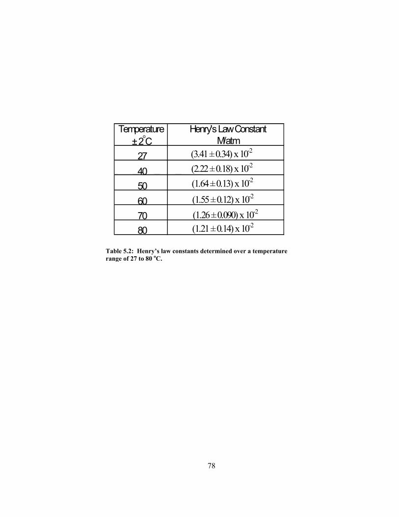
78

Table 5.2: Henry’s law constants determined over a temperature range of 27 to 80 oC.

Temperature Henry's Law Constant ± 2

o C M/atm

27 (3.41 ± 0.34) x 10-2

40 50 60 70 80

(2.22 ± 0.18) x 10-2

(1.64 ± 0.13) x 10-2

(1.55 ± 0.12) x 10-2

(1.26 ± 0.090) x 10-2

(1.21 ± 0.14) x 10-2

79

Temperature Henry's Law Constant ReferencesoC M/atm27 3.164 x 10-2 Lisal30 3.017 x 10-2 Harned

3.012 x 10-2 Harned2.837 x 10-2 Duan

40 2.400 x 10-2 Harned50 1.976 x 10-2 Harned

1.963 x 10-2 Harned60 1.043 x 10-2 Duan

Table 5.3: Henry’s law constants from the literature compared against calculated Henry’s law constants.

80

LIST OF REFERENCES

(1) Retallack, G. J. Carbon dioxide and climate over the past 300 Myr, Phil. Trans. R. Soc. Lond. A 2002, 360, 659. (2) Zeebe, R. E.; Wolf-Gladrow, D. CO2 in Seawater: Equilibrium, Kinetics, Isotopes; Elsevier Oceanography Series: New York, 2001. (3) Shirayama, Y.; Thornton, H. Effect of increased atmospheric CO2 on shallow water marine benthos, J. Geophys. Res. 2005, 110, C09S08. (4) Teng, H.; Yamasaki, A.; Shindo, Y. The fate of CO2 hydrate released in the ocean, Int. J. Energy Res. 1999, 23, 295. (5) Jena, N. R.; Mishra, P. C. An ab initio and density functional study of microsolvation of carbon dioxide in water clusters and formation of carbonic acid, Theor. Chim. Acta 2005, 114, 189. (6) Larsen, J.; Dahl-Jensen, D. Interior temperatures of the northern polar cap on Mars, Icarus 2000, 144, 456. (7) Miller, S. L.; Smythe, W. D. Carbon dioxide clathrate in the martian ice cap, Science 1970, 170, 531. (8) Longhi, J. Phase equilibrium in the system CO2-H2O: Application to Mars, J. Geophys. Res. 2006, 111, E06011. (9) Ferdows, M.; Ota, M. Molecular simulation study for CO2 clathrate hydrate, Chem. Eng. Technol. 205, 28, 168. (10) Teng, H.; Yamasaki, A. Pressure-mole fraction phase diagrams for CO2- pure water system under temperatures and pressures corresponding to ocean waters at depth to 3000 M, Chem. Eng. Commun. 2002, 189, 1485. (11) Maynard, B. Burning Questions about Gas Hydrates, Chemistry 2006, 27.

81

(12) Teng, H.; Yamasaki, A. Can CO2 hydrate deposited in the ocean always reach the seabed?, Energy Convers. Mgmt. 1998, 39, 1045. (13) Aya, I.; Yamane, K.; Yamada, N. Simulation experiment of CO2 Storage in the basin of deep ocean, Energy Convers. Mgmt. 1995, 36, 485. (14) Circone, S.; Stern, L. A.; Kirby, S. H.; Durham, W. B.; Chakoumakos, B. C.; Rawn, C. J.; Rondinone, A. J.; Ishii, Y. CO2 Hydrate: Synthesis, composition, structure, dissociation behavior, and a comparison to Structure I CH4 Hydrate, J. Phys. Chem. B 2003, 107, 5529. (15) E. Dendy Sloan, J. Clathrate Hydrates: The Other Common Solid Water Phase, Ind. Eng. Chem. Res. 2000, 39, 3123. (16) Uchida, T. Physical property measurements on CO2 clathrate hydrates. Review of crystallography, hydration number, and mechanical properties, Waste Management 1997, 17, 343. (17) Rudolph, W. W.; Fischer, D.; Irmer, G. Vibrational Spectroscopic Studies and Density Functional Theory Calculations of Speciation in the CO2- Water System, Appl. Spectrosc. 2006, 60, 130. (18) Maillet, J.-B.; Boutin, A.; Buttefey, S. From molecular clusters to bulk matter. I. Structure and thermodynamics of small CO2, N2, and SF6 clusters, J. Chem. Phys. 1998, 109, 329. (19) Koh, C. A. Towards a fundamental understanding of natural gas hydrates, Chem. Soc. Rev. 2002, 31, 157. (20) Subramanian, S.; E. Dendy Sloan, J. Trends in Vibrational Frequencies of Guests Trapped in Clathrate Hydrate Cages, J. Phys. Chem. B 2002, 106, 4348. (21) Englezos, P. Clathrate Hydrates, Ind. Eng. Chem. Res. 1993, 32, 1251. (22) E. Dendy Sloan, J. Clathrate Hydrates of Natural Gases, 2nd ed.; Marcel Dekker, Inc.: New York, New York, 1998. (23) E. Dendy Sloan, J. Gas Hydrates: Review of Physical/Chemical Properties, Energy Fuels 1998, 12, 191. (24) Khan, A. Theoretical studies of CO2(H2O)20,24,28 clusters: stabilization of cages in hydrates by CO2 guest molecules, J. Mol. Struct. (THEOCHEM) 2003, 664-665, 237.

82

(25) Falcke, H.; Eberle, S. H. Raman Spectroscopic Identification of Carbonic Acid, Water Res. 1990, 24, 685. (26) Abbott, T. M.; Buchanan, G. W.; Kruus, P.; Lee, K. C. 13C nuclear magnetic resonance and Raman investigations of aqueous carbon dioxide systems, Can. J. Chem. 1982, 60, 1000. (27) Waals, J. H. v. d.; Platteeuw, J. C. Clathrate Solutions; Interscience Publishers, Inc.: New York, 1959; Vol. II. (28) Ingle, James D.; Crouch, S. R. Spectrochemical Analysis; Prentice-Hall, Inc.: Upper Saddle River, NJ, 1988. (29) McCreery, R. L. Raman Spectroscopy for Chemical Analysis; John Wiley & Sons: New York, 2000. (30) Pelletier, M. J. Analytical Applications of Raman Spectroscopy; Blackwell Science Ltd: Malden MA, USA, 1999. (31) Smith, E.; Dent, G. Modern Raman Spectroscopy - A Practical Approach; John Wiley & Sons, Inc.: England, 2005. (32) Adams, W. A.; Greer, G.; Desnoyers, J. E.; Atkinson, G.; Kell, G. S.; Oldham, K. B.; Walkley, J. Chemistry and Physics of Aqueous Gas Solutions; The Electrochemical Society, Inc.: USA, 1975. (33) Harris, D. C.; Bertolucci, M. D. Symmetry and Spectroscopy: An Introduction to Vibrational and Electronic Spectroscopy; Dover Publications, Inc.: New York, 1978. (34) Cotton, F. A. Chemical Applications of Group Theory, 3rd ed.; John Wiley & Sons: New York, 1990. (35) Montero, S. Raman intensities of Fermi diads. I. Overtones in resonance with nondegenerate fundamentals, J. Chem. Phys. 1983, 79, 4091. (36) Anderson, A. The Raman Effect; Marcel Dekker, Inc.: New York, 1971. (37) Tejeda, G.; Mate, B.; Montero, S. Overtone Raman spectrum and molecular polarizability surface of CO2, J. Chem. Phys. 1995, 103, 568. (38) Frantz, J. D. Raman spectra of potassium carbonate and bicarbonate aqueous fluids at elevated temperatures and pressures: comparison with theoretical simulations, Chem. Geol. 1998, 152, 211.

83

(39) Wen, N.; Brooker, M. H. Ammonium Carbonate, Ammonium Bicarbonate, and Ammonium Carbamate Equilibria: A Raman Study, J. Phys. Chem. 1995, 99, 359. (40) Sato, H.; Matubayasi, N.; Nakahara, M.; Hirata, F. Which carbon oxide is more soluble? Ab initio study on carbon monoxide and dioxide in aqueous solution, Chem. Phys. Lett. 2000, 323, 257. (41) Uchida, T.; Takagi, A.; Mae, S.; Kawabata, J. Dissolution Mechanisms of CO2 Molecules in Water Containing CO2 Hydrates, Energy Convers. Mgmt 1997, 38, S307. (42) Sum, A. K.; Burruss, R. C.; E. Dendy Sloan, J. Measurement of Clathrate Hydrates via Raman Spectroscopy, J. Phys. Chem. B 1997, 101, 7371. (43) Roland, C. M.; Steele, W. A. Rotation-vibration CARS spectra of the 2v2 mode in CO2 gas, J. Chem. Phys. 1981, 74, 2733. (44) Fleyfel, F.; Devlin, J. P. FT-IR spectra of carbon dioxide clusters, J. Phys. Chem. 1989, 93, 7292. (45) Olijnyk, H.; Daufer, H.; Jodi, H.-J. Effect of pressure and temperature on the Raman spectra of solid CO2, J. Chem. Phys. 1988, 88, 4204. (46) Ikeda, T.; Mae, S.; Uchida, T. Effect of guest-host interaction on Raman spectrum of a CO2 clathrate hydrate single crystal, J. Chem. Phys. 1998,

108, 1352.

(47) Demetriou, M. D.; Ghoniem, N. M.; Lavine, A. S. Effects of nucleation transience on crystallization kinetics under strongly nonequilibrium conditions, J. Chem. Phys. 2002, 117, 10739. (48) Hirai, S.; Okazaki, K.; Tabe, Y.; Kawamura, K. CO2 clathrate-hydrate formation and its mechanism by molecular dynamics simulation, Energy Convers. Mgmt. 1997, 38, S301. (49) Sloan, E. D. Clathrate hydrate measurements: microscopic, mesoscopic, and macroscopic, J. Chem. Thermodyn. 2003, 35, 41. (50) Henning, R. W.; Schultz, A. J.; Thieu, V.; Halpern, Y. Neutron Diffraction Studies of CO2 Clathrate Hydrate: Formation from Deuterated Ice, J. Phys. Chem. A 2000, 104, 5066. (51) Kawamura, T.; Komai, T.; Yamamoto, Y.; Nagashima, K.; Ohga, K.; Higuchi, K. Growth Kinetics of CO2 hydrate just below melting point of ice, J. Cryst. Growth 2002, 234, 220.

84

(52) Buanes, T.; Kvamme, B.; Svandal, A. Computer Simulation of CO2 hydrate growth, J. Cryst. Growth 2006, 287, 491. (53) Gopalakrishnan, S.; Liu, D.; Allen, H. C.; Kuo, M.; Shultz, M. J. Vibrational spectroscopic studies of aqueous interfaces: salts, acids, bases, and nanodrops, Chem. Rev. 2006, 106, 1155. (54) Walrafen, G. E. Effects of equilibrium H-bond distance and angle changes on Raman intensities from water, J. Chem. Phys. 2004, 120, 4868. (55) Schicks, J. M.; Erzinger, J.; Ziemann, M. A. Raman spectra of gas hydrates-differences and analogies to ice Ih and (gas saturated) water, Spectrochim. Acta, Part A 2005, 61, 2399. (56) Devlin, J. P. Structure, specta, and mobility of low-pressure ices: Ice I, amorphous solid water, and clathrate hydrates at T<150 K, J. Geophys. Res. 2001, 106, 33333. (57) Someya, S.; Bando, S.; Chen, B.; Song, Y.; Nishio, M. Measurement of CO2 solubility in pure water and the pressure effect on it in the presence of clathrate hdyrate, Int. J. Heat Mass Transfer 2005, 48, 2503. (58) Portier, S.; Rochelle, C. Modelling CO2 solubility in pure water and NaCl- type waters from 0 to 300 OC and from 1 to 300 bar Application to the Utsira Formation at Sleipner, Chem. Geol. 2005, 217, 187. (59) Chapoy, A.; Mohammadi, A. H.; Chareton, A.; Tohidi, B.; Richon, D. Measurement and modeling of gas solubility and literature review of the properties for the carbon dioxide-water system, Ind. Eng. Chem. Res. 2004, 43, 1794. (60) Finlayson-Pitts, B. J.; James N. Pitts, J. Chemistry of the Upper and Lower Atmosphere: Theory, Experiments, and Applications; Academic Press: San Diego, CA, 1999. (61) Brown, T. L.; H. Eugene LeMary, J.; Bursten, B. E.; Burdge, J. R. Chemistry: The Central Science, 9th ed.; Pearson Education, Inc.: Upper Saddle River, NJ, 2003. (62) Harned, H. S.; Raymond Davis, J. The ionization constant of carbonic acid in water and the solubility of carbon dioxide in water and aqueous salt solutions from 0 to 50o, J. Am. Chem. Soc. 1943, 65, 2030.

85

(63) Duan, Z.; Sun, R.; Zhu, C.; Chou, I.-M. An improved model for the calculation of CO2 solubility in aqueous solutions containing Na+, K+, Ca2+, Mg2+, Cl-, and SO4

2-, Mar. Chem. 2006, 98, 131. (64) Lisal, M.; Smith, W. R.; Aim, K. Analysis of Henry's constant for carbon dioxide in water via Monte Carlo simulation, Fluid Phase Equilib. 2004, 226, 161. (65) Kaufmann, K. Choosing Your Detector. In OE Magazine, 2006. (66) Kaufmann, K. Light Levels and Noise. In Photonics Spectra, 2000; 149.

(67) McHale, Jeanne L. Molecular Spectroscopy; Prentice Hall: Upper

Saddle River, NJ, 1999. (68) Wendland, M.; Hasse, H.; Maurer, Experimental pressure vs. temperature data on three- and four-phase equilibria of fluid, hydrate and ice phases in the system carbon dioxide-water. G. J. Chem. Eng. Data 1999, 44, 901.

86

APPENDIX A

PHOTOMULTIPLIER TUBE EXPERIMENTS

A.1. Introduction

A shift of less than two wavenumbers is what distinguishes solvated CO2

vibrational modes from CO2 clathrate vibrational modes. Therefore, the detection system

must be very accurate. The Andor CCD camera that was originally used for the clathrate

experiments has a resolution of 7 cm-1 and does not have the accuracy needed. A more

accurate system is required to verify the experimental parameters used are sufficient to

form CO2 clathrates. One possible way to solve this problem is to use a photomultiplier

tube (PMT). A PMT has extremely high sensitivity and low noise compared to other

photosensitive devices. The high sensitivity and low noise could provide a better

resolution through a decrease of the slit widths. A brief discussion of the PMT follows.

A.2 PMT Background

A PMT (Figure A.1) is composed of a photoemissive cathode (photocathode), an

electron multiplier (dynodes), and an electron collector (anode) in a vacuum tube. The

PMT uses the photoelectric effect to convert optical photons into photoelectrons when

radiation enters the photocathode. These photoelectrons are emitted and accelerated

toward an increasingly more positive series of dynodes. The secondary electron emission

87

process that occurs at each dynode results in a “cascading effect” or amplification of

electrons.28,65,66

This amplification process results in a large charge packet at the anode for each

photoelectron collected by the first dynode. By the time the electrons have left the last

dynode and are collected at the anode, they have been amplified by a factor of 106. This

current amplification is also known as the gain.28 The gain, µ, is the average number of

electrons per anode pulse and depends highly on the power supply voltage, as shown in

Equation 1:

nn

n

Vn

A ααµ ⋅

+=

)1( (1)

where A is a constant, n is the number of dynodes, α is a constant determined by the

structure and material of the electrodes, and V is the supply voltage. Due to the high

internal gain, a PMT can detect low-level signals.

The PMT conversion efficiency or radiant sensitivity is dependent upon the

photocathode material. The dynodes are made of a secondary emission material that

establishes the energy threshold. If the photons entering the photocathode have energy

greater than the threshold energy, the photoelectrons escape the dynodes. The production

probability of photoelectrons emitted when one photon strikes the photocathode is called

the quantum efficiency28 and is shown in Equation 2

1001240×

×=

λSQE (2)

where S is the cathode radiant sensitivity in A/W at a given wavelength λ in nm. Due to

its dependence on wavelength, the photocathode chosen for this experiment must have

88

maximum quantum efficiency at 574 nm. The cathode radiant sensitivity and quantum

efficiency of the PMT used for experiments are shown in Figure A.2.

A.3. Experimental Setup

The experimental setup is shown in Figure A.3. A 532 nm continuous wave

(CW) laser (Spectra-Physics, Millennia II) was used to obtain spectra. A fiber optic

probe (InPhotonics, RP 532-05-15-FC) was used to both deliver the laser excitation

source to the sample and to collect the scattered light. The scattered light was delivered

to the entrance slit of a 500 mm monochromator (Acton Research, SpectraPro 500i) via a

200 µm collection fiber optic (InPhotonics, Inc.). The scatter was dispersed using a 1200

g/mm grating blazed at 500 nm, and data was collected to a photomultiplier tube

(Hamamatsu Photonics, R3896, multi-alkali, side-on, UV glass window). The voltage

was supplied to the PMT via a power supply (Spectral Products, AD110B Photobyte-P).

A virtual instrument program (LabVIEW 7.1) was used to collect and display the data.

Data was evaluated using Igor Pro (Wavemetrics, Version 4.0.5.1). Section A.4

describes the procedure used to optimize the PMT detection setup.

A.4. Determining the Experimental Parameters

The PMT was calibrated using the 475.8 nm line from a fluorescent light and the

wavenumber position was confirmed by taking a spectrum of naphthalene. The peak

positions of fluorescent light and naphthalene were compared to the literature values. 29

The fluorescent light spectrum was obtained using 200.0 µm entrance and exit slit widths

and a spectral range of 575 to 579 nm (Figure A.4). The 1382 cm-1 peak of naphthalene

89

(Figure A.5) was obtained with 100.0 µm entrance and exit slit widths over a spectral

range of 574 to 578 nm. A 0.01 nm step size, and a PMT integration period consisting of

1,000 scans was used for both spectra.

The gain to be used for the experiments was determined by obtaining spectra of

naphthalene with 150.0 µm entrance and exit slit widths. The spectral range covered 574

to 577 nm. A 0.5 nm step size and a PMT integration period consisting of 500 scans

were used. Gains of 2, 4, 8, and 16 were tested, Figure A.6. As the gain increased, the

S/N ratio improved. It was concluded that a gain of 16 resulted in the best S/N and

would be used for future PMT experiments.

Initial solvated CO2 spectra were obtained using a spectral region of 572 to 576

nm with a 0.20 nm step size. A PMT integration period of 1000 scans was used. A

stainless steel cell was filled with 100.0 mL of nano-pure water (18.2 MΩ • cm). A

pressure transducer (MKS PDR2000 Dual Capacitance Manometer) was used to verify

the cell pressure was maintained at 12.73 atm. The entrance and exit slits were adjusted

simultaneously to determine the appropriate slit width to be used for experiments. A

solvated CO2 peak was not observed until slit widths of 500 µm were reached. (Figure

A.7) A reproducible peak was not observed until 650 µm due to low S/N.

A resolution experiment was performed to determine if 650 µm slit widths

provided a better resolution than the CCD camera. The resolution of the PMT was

determined by using the 1382 cm-1 peak of naphthalene. The step size was 0.01 nm and

the spectral range covered 572 to 576 nm. A PMT integration period consisting of 1,000

scans was used. The entrance and exit slits were adjusted from 30.0 µm to 450.0 µm,

simultaneously. The data was fit with a Voigt function. The FWHM of the 1382 cm-1

90

peak was determined for each slit width, Figure A.8. The FWHM was plotted as a

function of the slit width. For slit widths below 50 µm, a poor fit due to low S/N resulted

in inaccurate FWHM determinations. The near level slope at 5 cm-1 shows the FWHM is

nearly constant for several slit widths indicating this FWHM is the minimum resolution.

In addition, the slope indicates a slit width below 100 µm will not improve the resolution.

The 100 µm slit width was used for experiments.

Further reduction of the slit width was attempted by increasing the integration period

of the PMT and by taking the average of several spectra. It was hoped that increasing the

integration period and taking an average of ten to seventeen spectra would enhance the

S/N. The integration period of the PMT was adjusted from 1,000 scans to 100,000 scans.

For each integration period, a spectrum was acquired using a 450 µm slit width and a 0.5

nm step size. The data was fit with a Voigt function. Although increasing the integration

period of the PMT improved the S/N slightly, the integration time increased from minutes

to hours, Figure A.9.

Experiments were done varying the PMT integration period from 100 scans to 1,000

scans while averaging ten spectra. The experimental parameters remained the same.

Standard deviations of the averages were calculated and are shown in the plots.

Obtaining an average of several spectra (Figure A.10) with shorter integration periods

actually improved the S/N more than just varying the integration time but still not enough

to reduce the slit width.

Neither increasing the PMT integration time nor averaging the spectra decreased the

slit width to the needed 100 µm indicated by the resolution study. The last experiment to

decrease the slit width involved increasing the laser energy from 148 mW to 201 mW.

91

The slit width was set at 100 µm and a step size of 0.1 nm was used. The PMT

integration was 10,000 scans and seventeen spectra were averaged. The resulting spectra

indicated solvated CO2 peaks could be observed with an input laser energy of 201 mW.

Standard deviations of the averages were calculated and are shown in Figure A.11.

Energies below 201 mW were insufficient at 100 µm to observe a solvated CO2 peak.

Since such a high energy was required to obtain data, it was necessary to determine if

the energy required to obtain data would destroy the sample. The CCD camera was used

with a shorter integration time of 90 s due to its improved S/N. A slit width of 50 µm and

a 1200 g/mm grating were used to acquire the spectrum. SpectraSense software (Acton

Research, version 4.2.9) acquired spectra. An input of energies from 77 mW to 180 mW

was used. The stainless steel cell was filled with 100.0 mL of nanopure water (18.2

MΩ • cm). The cell was kept at -15 ± 2 0C and allowed to freeze. During the experiment,

the cell temperature was maintained while the cell was exposed to the laser for the entire

experiment. The stretching region of H2O(s) (2900–3800 cm-1) was evaluated for up to

three hours. A decrease in intensity of the ~3051 cm-1 peak and an increase in the ~3300

cm-1 peak would indicate the ice was melting. Refer to Chapter 3 for vibrational

assignments. However, even at the highest energy the shape of the peaks did not change

for three hours indicating the laser energy was not sample destructive, Figure A.12.

A.5. Conclusion

Data obtained with the PMT and LabVIEW VI is reproducible and indicates the

PMT setup works correctly. However, the resolution was not improved over the use of

92

the Roper Scientific CCD camera. The Roper Scientific monochromator with CCD

camera will be used in future experiments.

93

Figure A.1: Diagram of the R3896 PMT with a closeup of the dynodes. (www.sales.hamamatsu.com)

94

Figure A.2: The cathode radiant sensitivity (blue) and the quantum efficiency (red) of the R3896 PMT at 574 nm. (www.sales.hamamatsu.com)

95

j

b a

c d

e

f

g h

i

kl

Figure A.3: Schematic of PMT Raman setup: (a) computer; (b) Spectra-Physics Millenia II laser; (c) stainless steel cell; (d) gas inlet valve; (e) gas outlet valve; (f) fiber optic Raman probe; (g) monochromator; (h) photomultipler tube; (i) AD110B power supply; (j) A/D connector; (k) MKS PDR2000 Dual Capacitance Manometer; (l) pressure transducer. The inset shows a picture of the R3896 PMT. (www.sales.hamamatsu.com)

96

Figure A.4: Spectrum of fluorescent light showing the 577 and 579 nm lines obtained with a 200 µm slit width, a 0.01 nm step size, and a PMT integration period consisting of 1000 scans. The spectral fit is shown in blue.

80

60

40

20

0

Inte

nsity

(A.U

.)

579578577576575Wavelength (nm)

97

Figure A.5: Spectrum of naphthalene showing the 1382 cm-1 peak. The spectrum was obtained using a 100 µm slit width, a 0.01 nm step size, and a PMT integration period consisting of 1000 scans. The spectral fit is shown in blue.

0.6

0.5

0.4

0.3

0.2

0.1

Inte

nsity

(A.U

.)

1440142014001380136013401320Raman Shift (cm-1)

98

Figure A.6: Naphthalene spectra were evaluated with varying gains, a 0.5 nm step size, and a PMT integration period consisting of 500 scans. The red lines indicate the 1390 and 1465 cm-1 peaks. As the gain increased, the S/N increased. The data are offset for easier observation.

2.5

2.0

1.5

1.0

0.5

0.0

Inte

nsity

(A.U

.)

148014601440142014001380Raman Shift (cm-1)

x2

x4

x8

x16

99

0.5

0.4

0.3

0.2

0.1

Inte

nsity

(A.U

.)

1440142014001380136013401320Raman Shift (cm-1)

80 µm

100 µm

300 µm

500 µm

600 µm

650 µm

Figure A.7: Solvated CO2 spectra acquired using the PMT while varying the entrance and exit slits, simultaneously. A PMT integration period consisting of 1000 scans and a 0.2 nm step size was used to acquire spectra. The red line highlights the solvated CO2 peak position at 1390 cm-1. The data are offset for easier observation.

100

25

20

15

10

5

0

FWH

M (c

m-1

)

5004003002001000Slit Width (um)

Figure A.8: The FWHM of the 574 nm line of napthalene as a function of the slit width. Resolution was determined from the plot. Spectra were obtained using a 0.01 nm step size and a PMT integration period consisting of 1000 scans. The near level slope (red) indicates the minimum resolution of the PMT while the positive slope (black) indicates the resolution at other slit widths.

101

Figure A.9: Spectra of the solvated CO2 peak obtained with a 450 um slit width and a 0.5 nm step size with PMT integration periods consisting of (a) 1,000, (b) 50, 000, and (c) 100,000 scans. The spectral fit is shown in blue.

80x10-3

60

40

20

0

Inte

nsity

(A.U

.)

1440142014001380136013401320Raman Shift (cm-1)

c) 100,000

80x10-3

60

40

20

0

Inte

nsity

(A.U

.)

1440142014001380136013401320Raman Shift (cm-1)

a) 1,000

80x10-3

60

40

20

0

Inte

nsity

(A.U

.)

1440142014001380136013401320Raman Shift (cm-1)

b) 50,000

102

Figure A.10: Spectra of solvated CO2 determined by averaging 10 spectra using different PMT integration periods consisting of (a) 100 Scans, (b) 500 Scans, and (c) 1,000 Scans. The spectra were obtained with a 450 um slit width and a 0.5 nm step size. The fits are shown in blue. Standard deviation error bars of the average are shown.

0.30

0.25

0.20

0.15

0.10

0.05

0.00

Inte

nsity

(A.U

.)

1440142014001380136013401320Raman Shift (cm-1)

a) 100

0.30

0.25

0.20

0.15

0.10

0.05

0.00

Inte

nsity

(A.U

.)

1440142014001380136013401320Raman Shift (cm-1)

b) 500

0.30

0.25

0.20

0.15

0.10

0.05

0.00

Inte

nsity

(A.U

.)

1440142014001380136013401320Raman Shift (cm-1)

c) 1000

103

Figure A.11: Spectra of solvated CO2 obtained with a PMT integration period consisting of 10,000 scans and an average of 17 spectra was used at laser energies of (a) 148 mW and (b) 201 mW. The spectra were obtained with a slit width of 100 um and a step size of 0.1 nm. The standard deviation error bars of the average are shown. A solvated CO2 peak is observed in (b) only, and its spectral fit is shown in blue.

0.30

0.25

0.20

0.15

0.10

0.05

0.00

Inte

nsity

(A.U

.)

14601440142014001380136013401320Raman Shift (cm-1)

a) 148 mW

0.30

0.25

0.20

0.15

0.10

0.05

0.00

Inte

nsity

(A.U

.)

14601440142014001380136013401320Raman Shift (cm-1)

b) 201 mW

104

Figure A.12: The stretching region of H2O(s) exposed to (a) 77 mW and (b) 180 mW laser energy for up to 3 hours. The spectra were obtained with the CCD camera with an integration time of 90 s, a 1200 g/mm grating, and a 50 um slit width.

4000

3000

2000

1000

0

Inte

nsity

(A.U

.)

3600340032003000Raman Shift (cm-1)

0 min 30 min 1 hr 3 hr

b) 180 mW

4000

3000

2000

1000

0

Inte

nsity

(A.U

.)

3600340032003000Raman Shift (cm-1)

0 min 60 min

a) 77 mW

105

APPENDIX B

PHOTOMULTIPLIER TUBE LABVIEW 7.1

B.1. Introduction

This appendix describes the LabVIEW 7.1 VI program used to obtain Raman

spectra using a photomultiplier tube with a monochromator. The 500i PMT VI program

allows communication between two instruments, the Spectral Products AD110B

Photobyte-P PMT Detection System and the SpectraPro 500i Monochromator. This

program is designed to easily obtain a spectrum by utilizing a scan setup with continuous

data acquisition. A time delay is used to control the number of scans obtained at a set

collection frequency. All spectra are individually saved as a dat file.

This LabVIEW VI program is a modified version of the one originally written by

Gibum Kim and Paul Cremer from Texas A&M University. Dr. Dingfang Liu of the

Allen Lab modified the LabVIEW VI program for using the AD110B Photobyte-P PMT

detection system with other instruments in the laboratory. Modifications for use with the

500i monochromator were done with the assistance of Chris Beekman of the Allen Lab.

An AD110B VI program developed by Spectral Products was modified and inserted into

the 500i PMT VI program. Acton Research supplied the monochromator drivers.

106

B.2. Using the 500i PMT VI

This section explains the steps that must be followed to accurately collect data

with the 500i PMT VI program. The monochromator must be turned on before opening

the program, or it will not be recognized by the program.

1. Open SpectraSense. Go to Hardware Setup. The mirror position must be

changed so the light is directed into the PMT instead of the CCD camera. On the

monochromator image, two exit slits will be observed. Click on the exit slit that

corresponds to the PMT. A click will be heard in the monochromator. The arrow

direction will appear as shown in Figure B.1. To return to the CCD camera, click

on the corresponding exit slit, and the arrow direction will appear as shown in

Figure B.2.

2. Select appropriate grating.

3. Manually open the entrance slit by placing a checkmark in the box beside open.

4. Close SpectraSense.

5. Open 500i PMT VI. The Front Panel is shown in Figure B.3. The Block

Diagram is shown in Figure B.4.

6. Press the stop button on the navigation bar on the Front Panel because the

program automatically runs when opened.

Front Panel Setup for the 500i PMT VI

All white boxes on the Front Panel require user input.

107

1) SCAN SETUP

7. Verify the Scan Mode is set at Scan. The 500i PMT VI program is designed to

halt data collection if set at Fixed.

8. Enter the starting wavelength in Begin nm. Enter the final wavelength in End nm.

The scan is designed to stop one wavelength past the End nm.

9. Indicate the number of scans to be obtained per nm in Scans per nm.

10. Enter the step increment to be used in nm steps, i.e. if 10 points per nm is needed,

enter 0.10.

11. Enter the number of scans to be obtained in Scans to run.

12. The Scan Delay is used to prevent continuous running of the program. Insert the

time (in milliseconds) between scans.

2) FILE SETUP

13. Under Directory, enter where the data is to be stored. The C drive is best for the

programs used to display the data. Also, include the common name of the

spectra, i.e. C:\Ashley\napth where “C:\Ashley” is the location and “napth” is the

common name of the spectra.

3) PMT SETUP

14. The Gain may be adjusted to whatever gain the user desires. The default is set at

x2, but x16 is recommended.

15. Set the Voltage Setting to ~900 V. The maximum voltage is dependent upon the

PMT used. With the R3896 PMT, the maximum is 1000 V.

16. Under Scans, indicate the number of scans.

17. Open the laser shutter and turn on the PMT power supply.

108

18. Press the single arrow on the navigation bar at the top of the Front Panel to begin

the scan.

Running 500i PMT VI Program

An update box is located between the PMT SETUP and the SCAN CONTROL boxes.

A number of gray boxes, or indicators, verify the program is correctly controlling the

monochromator. These indicators are vital to the program so a description follows:

19. Points indicates how many data points will be taken and plotted for each scan.

20. Set Mono Wavelength indicates at what wavelength the monochromator grating

has been set. At the beginning of each scan, it will default to the begin nm and

will auto-increment by the number entered in nm steps.

21. Current NM is the wavelength to which the monochromator is set. This is to

verify the monochromator is working correctly and is vital to the program. If a

–1.000 is observed instead of the number inserted into Set Mono Wavelength, the

monochromator is not communicating effectively. The computer may need to be

rebooted and/or the monochromator turned off.

22. Elapsed Time indicates the duration of the scan.

23. Scans Completed keeps the user informed of the progress of the scans.

24. The Actual PMT Voltage shows the voltage of the PMT after the scan is

completed.

25. Data shows the signal voltage values.

26. AVG is the data point to be plotted for that wavelength. It is the average of all the

PMT scans (i.e. 1000) and should correspond to the voltage from Data.

109

Figure B.1: SpectraSense monochromator diagram showing the laser path is towards the PMT.

110

Figure B.2: SpectraSense monochromator diagram showing the laser path is towards the CCD camera.

111

Figure B.3: Front Panel of the 500i PMT VI

112

Figure B.4: Block diagram of the 500i PMT VI

113

APPENDIX C

ANALYZING SPECTRASENSE SPECTRA IN IGOR PRO 4.0.5.1

C.1. Introduction This appendix describes the Igor Pro (Wavemetrics, Version 4.0.5.1) macro used

to analyze the Raman spectra acquired using SpectraSense (Acton Research, Version

4.2.9). The Raman macro was written by Lisa Van Loon of the Allen Lab to use with

SpectraSense. The macro is designed to load individually saved spectra into one graph

and table. Background subtracted spectra is provided as an option.

C.2. Using the Raman Macro This section explains the steps that must be followed to accurately graph spectra. 1) Selecting Procedure

1. Open IgorPro. Go to File.

2. Go to Open File.

3. Select Procedure.

4. Browse for Raman.ipf.

5. Select Raman.ipf.

6. Set limM equal to number of spectra minus one.

2) Napthalene Spectrum

114

7. Specify the file location where spectra are stored in NewPath/O path “_”, i.e.

“C:Ashley:08.10.06:”. Colons are used to separate files.

8. For filename, insert the default name SpectraSense is using. Use the

naphthalene spectrum, i.e. "napth.arc_data"

3) Raw Data

9. Specify the file location where spectra are stored in NewPath/O path “_”, i.e.

“C:Ashley:08.10.06:”. This should be the same location as naphthalene.

10. For basefile, indicate the common file name. This name is set in SpectraSense

before acquisition, i.e. “clathrate1”

11. For filename, insert the default name used by SpectraSense. Use only the

initial spectra, i.e. "clathrate1_001_Area01.arc_data"

4) Running the Raman Macro

12. To run macro, type Raman() into the command line of the command window.

13. Press Enter.

5) Background Subtraction Option

14. Repeat Step B. Use the background file instead of the naphthalene file.

15. Repeat Step C.

16. Delete the “//” inserted in the macro command: wave1=wave1// - bkgd

17. Repeat Step D.

The Raman macro written to analyze spectra acquired with SpectraSense is shown

below:

#pragma rtGlobals=1 // Use modern global access method. #include <Waves Average> Macro raman()

115

Silent 1 KillWaves/A/Z string filename, wave0name, wave1name, basefile,xaxisname, bkgdcorrected string numstring variable /g m, limM m = 0 limM =100 // number of sample spectra minus one NewPath/O path "c:ashley:08.10.06:" //specify file location filename = "naphth.arc_data" //specify background file name LoadWave/G/A/P = path filename Rename wave0, wavenumbers Rename wave1, bkgd Edit wavenumbers, bkgd //starts table Display bkgd vs wavenumbers as "bkgd" NewPath/O path "c:ashley:08.10.06:" //specify file location basefile="clathrate1" //specify the common file name filename = "clathrate1_001_Area01.arc_data" //change this to match the data file name Raman: loading the initial spectrum LoadWave/G/A/P=path filename do sprintf numstring, "%03d", (m+1) filename = basefile + "_" + numstring + "_Area01.arc_data" LoadWave/G/A/P=path filename wave1=wave1// - bkgd //to load waves with no bkgd correction remove -bkgd wave0name = basefile + num2str(m+1) + "cm-1" wave1name = basefile + num2str(m+1) + "au" Rename wave0, $wave0name Rename wave1, $wave1name AppendtoTable $wave1name if (m == 0) then Display $wave1name vs wavenumbers as "data"

116

else Append $wave1name vs wavenumbers endif ModifyGraph rgb($wave1name)=(10000,5000,m*100) ModifyGraph tick(left)=2,mirror(left)=1,minor(left)=0,notation(left)=1 ModifyGraph font(left)="Arial" Label left "Intensity (A.U.)" ModifyGraph tick=2,mirror=1,minor=0,font="Arial" Label bottom "Raman Shift (cm\\S-1\\M)" ModifyGraph minor=1 SetAxis bottom 1200, 1500 m = m + 1 while (m<limM) end