
Ramachandra T.V. Subash Chandran M.D Joshi N.V.
156
Sahyadri Conservation Series 35 Influence of Landscape Dynamics on Hydrological Regime in Central Western Ghats Ramachandra T.V. Subash Chandran M.D Joshi N.V. Sreekantha Saira Varghese K. Vishnu D.M. Western Ghats Task Force, Government of Karnataka Karnataka Biodiversity Board, Government of Karnataka The Ministry of Science and Technology, Government of India The Ministry of Environment and Forests, Government of India ENVIS Technical Report: 65 December 2013 Environmental Information System [ENVIS] Centre for Ecological Sciences, Indian Institute of Science, Bangalore - 560012, INDIA Web: http://ces.iisc.ernet.in/energy/ http://ces.iisc.ernet.in/biodiversity Email: [email protected], [email protected]
Transcript of Ramachandra T.V. Subash Chandran M.D Joshi N.V.

Sahyadri Conservation Series 35
Influence of Landscape Dynamics on
Hydrological Regime in Central Western Ghats
Ramachandra T.V. Subash Chandran M.D Joshi N.V.
Sreekantha Saira Varghese K. Vishnu D.M.
Western Ghats Task Force, Government of Karnataka
Karnataka Biodiversity Board, Government of Karnataka
The Ministry of Science and Technology, Government of India
The Ministry of Environment and Forests, Government of India
ENVIS Technical Report: 65
December 2013
Environmental Information System [ENVIS]
Centre for Ecological Sciences,
Indian Institute of Science,
Bangalore - 560012, INDIA Web: http://ces.iisc.ernet.in/energy/
http://ces.iisc.ernet.in/biodiversity Email: [email protected],

ENERGY AND WETLANDS RESEARCH GROUP, CES TE15
CENTRE FOR ECOLOGICAL SCIENCES,
New Bioscience Building, Third Floor, E Wing
Near D Gate, INDIAN INSTITUTE OF SCIENCE, BANGALORE 560 012
Telephone: 91-80-22933099/22933503 extn 107 Fax: 91-80-23601428/23600085/23600683[CES-TVR]
Email: [email protected], [email protected] Web: http://ces.iisc.ernet.in/energy http://ces.iisc.ernet.in/biodiversity Open Source GIS: http://ces.iisc.ernet.in/grass

Influence of Landscape Dynamics on Hydrological Regime in Central Western Ghats
Ramachandra T.V. Subash Chandran M.D. Joshi N.V.
Saira Varghese K.
Western Ghats Task Force, Government of Karnataka
Karnataka Biodiversity Board, Government of Karnataka
The Ministry of Science and Technology, Government of India
The Ministry of Environment and Forests, Government of India
Sahyadri Conservation Series: 35
ENVIS Technical Report: 65
December 2013
Environmental Information System [ENVIS] Centre for Ecological Sciences,
Indian Institute of Science, Bangalore-560012.

Ramachandra T.V., Subash Chandran M.D., Joshi N.V., Sreekantha, Saira V.K and
Vishnu D.M., 2013. Influence of Landscape Dynamics on Hydrological Regime in
Central Western Ghats Sahyadri Conservation Series 35, ENVIS Technical Report 65,
CES, Indian Institute of Science, Bangalore 560012, India 1
Sahyadri Conservation Series: 35
Influence of Landscape Dynamics on Hydrological Regime in Central Western Ghats
I Landscape dynamics in Sharavathi river basin 1
Summary 2
Introduction
Hydrological Cycle
Water: Soil and Plant Interactions
Plant Water Use
Water and Soil
Hydrological and Other Functions of tropical trees
Crop Water Need
Landuse/Landcover Change and Its Effect on the
Hydrological Cycle
Use of Remote Sensing and GIS Techniques in Hydrology
3
Objectives 14
Review of Literature 16
Study Area 41
Data and Methods 53
Results and Discussions 69
Conclusions 113
References 115
II Landscape dynamics on hydrologic regime in Aghnashini river basin 128
Appendix I: Vegetation Characteristics of Western Ghats
148

Ramachandra T.V., Subash Chandran M.D., Joshi N.V., Sreekantha, Saira V.K and
Vishnu D.M., 2013. Influence of Landscape Dynamics on Hydrological Regime in
Central Western Ghats Sahyadri Conservation Series 35, ENVIS Technical Report 65,
CES, Indian Institute of Science, Bangalore 560012, India 2
Sahyadri Conservation Series: 35
Influence of Landscape Dynamics in a River Basin
on Hydrological Regime
Summary
Pristine forests rich in flora and fauna are being cleared especially in the tropical areas to meet
the growing demand of burgeoning populations. This has given rise to concerns about land
use/land cover changes with the realization that land processes influence climate. Studies have
further indicated its impact on the hydrological cycle and thus the water budget of a region.
The present study is an attempt to quantify the hydrological components using Sharavathi river
basin as a case study and to determine its changes over time using remote sensing and GIS.
Western Ghats region is species rich with a fair degree of endemism in both flora and fauna. A
dam was put across the Sharavathi River in 1964 for harnessing electricity. Over the years there
have been changes in the land use/land cover owing partly due to unplanned anthropogenic
activities subsequent to setting up of the dam. This study explores and quantifies the
hydrological parameters that have altered due to large scale land use and land cover changes.
In this regard, satellite data has offered excellent inputs to monitor dynamic changes through
repetitive, synoptic and accurate information of the changes in a river basin. It also provided a
means of observing hydrological state variables over large areas, which was useful in parameter
estimation of hydrologic models. GIS offered means for merging various spatial themes (data
layers) that was useful in interpretation, analysis and change detection of spatial structures and
objects. Studies reveal the linkages among variables such as land use, hydrology and ecology.
Regions with significant forest cover and low anthropogenic activities resulted in lesser runoff,
higher recharge and thus higher yield to stream resulting in perennial streams whereas regions
with poor forest cover and higher anthropogenic activities showed higher runoff, significant
reduction of recharge and thus lower yield to streams resulting in ephemeral streams.
Keywords: Hydrology, Western Ghats, Land use, Land cover, Biodiversity

Ramachandra T.V., Subash Chandran M.D., Joshi N.V., Sreekantha, Saira V.K and
Vishnu D.M., 2013. Influence of Landscape Dynamics on Hydrological Regime in
Central Western Ghats Sahyadri Conservation Series 35, ENVIS Technical Report 65,
CES, Indian Institute of Science, Bangalore 560012, India 3
Sahyadri Conservation Series: 35
1.0 Introduction
There has been a growing need to study, understand and quantify the impact of major land use
changes on hydrologic regime, in terms of both water quantity and quality. Land use influences
catchment hydrological responses by partitioning rainfall between return flow to the
atmosphere as evaporation and transpiration (“green water”) and flow to aquifers and rivers
(“blue water”) (Hope et al. 2003). Increasing attention is now being paid to understanding the
dynamic inter-relationships between “green” and “blue” water, as these are considered to
underpin essential terrestrial and aquatic ecosystem services (Falkenmark, 2003). FAO
suggests that almost all “green” water and a large proportion of “blue” water are needed to
sustain ecosystem structures and functions, and maintain sustainable water supplies. For
example, conversion of grassland and forests to pasture, plantations and arable land alters the
hydrological response of a catchment by modifying the various physical processes such as
infiltration rates, evaporation and runoff.
Developing countries in the tropics are facing threats of rapid deforestation due to unplanned
developmental activities based on ad-hoc approaches and also due to policies and laws that
considers forest as national resource to be fully exploited. Anthropogenic activities coupled
with skewed policies have resulted in the disappearance of pristine forests and wetlands in the
form of logging, afforestation by plantation trees, dam constructions, and conversion of lands
for other uses. Agricultural activities have led to a widespread deterioration in soil structures,
a process that causes soil sealing and crusting, and reduced rates of infiltration and soil storage.
Various studies (Sikka, et al. 1998, Van Lill et al. 1980; Scott and Lesch, 1997) provide
evidence to support the supposition that land use changes, involving conversion of natural
forests to other land uses agriculture (enhanced grazing pressure and intensive cultivation
practices) and plantation (widespread acacia and eucalyptus planting) have led to soil
compaction, reduced infiltration, groundwater recharge and discharge, and rapid and excessive
runoff. These structural changes in the ecosystem will influence the functional aspects namely
hydrology, bio-geo chemical cycles and nutrient cycling. These are evident in many regions in
the form of conversion of perennial streams to seasonal and disappearance of water bodies
leading to a serious water crisis. Thus, it is imperative to understand the causal factors
responsible for changes in order to improve the hydrologic regime in a region. It has been
observed that the hydrological variables are complexly related with the vegetation present in
the catchment. The presence or absence of vegetation has a strong impact on the hydrological
cycle. This requires understanding of hydrological components and its relation to the land
use/land cover dynamics. The reactions or the results are termed hydrological response and
depends on the interplay between climatic, geological and land use variables. Hydrological
responses can be understood by analysing land use changes using temporal remote sensing data

Ramachandra T.V., Subash Chandran M.D., Joshi N.V., Sreekantha, Saira V.K and
Vishnu D.M., 2013. Influence of Landscape Dynamics on Hydrological Regime in
Central Western Ghats Sahyadri Conservation Series 35, ENVIS Technical Report 65,
CES, Indian Institute of Science, Bangalore 560012, India 4
Sahyadri Conservation Series: 35
and traditional approaches. Traditional approaches considers spatial variability by dividing a
basin into smaller geographical units such as sub-basins, terrain-based units, land cover classes,
or elevation zones on which hydrological model computations are made, and by aggregating
the results to provide a simulation for the basin as a whole. Modelling is thus simplified because
areas of the catchment within these units are assumed to behave similarly in terms of their
hydrological response. Remote sensing and GIS techniques have been used to determine some
of the model parameters. The main applications of remote sensing in hydrology are to 1)
determine watershed geometry, drainage network and other map type information for
hydrological models 2) provide input data such as land use/land cover, soil moisture, surface
temperature etc. GIS on the other hand allows for the combination of spatial data such as
topography, soil maps and hydrologic variables such as rainfall distribution or soil moisture.
But prior to modelling, it is necessary to get a complete understanding of the hydrological cycle
operating in a river basin. The following section deals with the description of the cycle and the
water balance equation.
1.1. Hydrological Cycle: Water is constantly circulated between earth and atmosphere. This
global circulation is accomplished by the heat of the sun and the pull of gravity.
Precipitation is water released from the atmosphere in the form of rain, snow, sleet or hail.
During precipitation, some of the moisture is evaporated back into the atmosphere before
reaching the ground. Some precipitation is intercepted by plants, a part of it infiltrates the
ground, and the remainder flows off the land into lakes, rivers or oceans. Some may be
directly evaporated if adequate transfer from the soil to the surface is maintained. This
occurs where a high groundwater table (free water surface) is within the limits of capillary
transport to the ground surface. Water that is infiltrated replenishes soil moisture
deficiencies and enters storage provided in groundwater reservoirs, which in turn
maintains dry weather stream flow. Vegetation using water from soil and groundwater
returns the infiltrated water into the atmosphere by transpiration. Water that is stored in
depressions will eventually evaporate or infiltrate into the ground. Surface runoff reaches
minor channels (gullies, rivulets and the like), flows to major streams and rivers and
finally reaches the ocean. Along the course of a stream, evaporation and infiltration can
also occur (Viessman et al., 1989).
Figure 1.1: Hydrological Cycle

Ramachandra T.V., Subash Chandran M.D., Joshi N.V., Sreekantha, Saira V.K and
Vishnu D.M., 2013. Influence of Landscape Dynamics on Hydrological Regime in
Central Western Ghats Sahyadri Conservation Series 35, ENVIS Technical Report 65,
CES, Indian Institute of Science, Bangalore 560012, India 5
Sahyadri Conservation Series: 35
Even though the hydrological cycle is continuous in nature, it is not uniform throughout the
world: the residence time of water varies often dramatically among different portions of the
cycle. Fig.1.1 depicts a hydrological cycle. In addition to the variability in residence time, the
processes associated with the hydrologic cycle are not evenly distributed throughout the world.
The hydrological cycle is defined as a closed system whereby there is no mass or energy created
nor lost within it. In this case, the mass under consideration is water. This can be represented
by an equation, which is normally termed as the water balance equation. The basic form of the
equation is as follows:
I = O S (1.1)
where,
I – input, O-output and S –change in storage
or
P R ET EGWRGWDS Q = 0 (1.2)
Where,
P –precipitation, R- runoff, T- transpiration from vegetation E – evaporation from open water
(reservoirs or lakes) and soil, GWR- groundwater recharge, GWD- groundwater discharge; Q
– runoff, S- change in storage.
1.2 Water: Soil and Plant Interactions: Water is one of the most common and most
important substances on the earth’s surface. It is essential for the existence of life, and the kinds
and amounts of vegetation occurring on the various parts of the earth’s surface depend more
on the quantity of water available than on any other single environmental factor. It is important
quantitatively as well as qualitatively, constituting 80-90% of the fresh weight of most
herbaceous plant parts and over 50% of the fresh weight of woody plants. The ecological
importance of water is the result of its physiological importance (Kramer, 1983). The only way
in which an environmental factor such as water can affect plant growth is by physiological
processes. Figure 1.2 describes the quantity and quality of plant growth controlled by hereditary
potentialities and environmental factors, operating through the internal processes and
conditions of plants.
1.2.1 Plant Water Use: Plants use water in biochemical reactions, as a solvent and to
maintain turgor, but most of the water taken up by plants is transpired to the atmosphere.
Globally, plants recycle more than half of the ~110 000 km3/yr of precipitation that falls on
land each year. Transpired water moves from soil to plant to atmosphere along a continuum of

Ramachandra T.V., Subash Chandran M.D., Joshi N.V., Sreekantha, Saira V.K and
Vishnu D.M., 2013. Influence of Landscape Dynamics on Hydrological Regime in
Central Western Ghats Sahyadri Conservation Series 35, ENVIS Technical Report 65,
CES, Indian Institute of Science, Bangalore 560012, India 6
Sahyadri Conservation Series: 35
increasingly negative water potential, flowing ‘downhill’ thermodynamically but ‘uphill’
physically from root to shoot.
Figure 1.2: Hereditary Potentialities and Environmental Factors Operating
through Plants
Plants get water from the soil through roots. This water then passes through the stem, leaves
and into the atmosphere. The following sections will briefly describe each process.
Movement through Soil: Root hairs make intimate contact with soil particles and greatly
amplify the surface area that can be used for water absorption by the plant (Taiz and Zeiger,
2002). Figure 1.3 depicts the contact surfaces between root hair and soil. Soil is a mixture of
sand, clay and silt, water, dissolved solutes and air and sometimes organic matter. As the plant
adsorbs water, the soil solution recedes into smaller pores and interstices between the soil
particles. At the air-water interface, this recession causes the surface of the soil solution to
develop concave menisci and brings the solution into tension. As more water is removed from
soil, the menisci become more acute resulting in greater tension (negative pressures). As the
Hereditary Potentialities
1. Depth and extent of root
systems
2. Size, shape and total area of
leaves and ratio of internal to
external surface
3. Number, location and behavior
of stomata
Environmental factors
1. Soil-texture, structure, depth, chemical composition,
pH, water holding capacity, hydraulic conductivity
2. Atmospheric- amount and distribution of precipitation
3. Ratio of precipitation to evaporation
4. Radiant energy, wind, vapour pressure and other
factors affecting evaporation and transpiration
Plant Processes and Conditions
1. Water absorption
2. Ascent of sap
3. Transpiration
4. Internal water balance reflected in water potential, turgidity,
stomatal openings and cell enlargements
5. Effects on photosynthesis, carbohydrate and nitrogen metabolism
and other metabolic processes
Quantity and Quality of Growth
1. Size of cells, organs and plants
2. Dry weight, succulence, kinds and amounts of various
amounts of various compounds and accumulated
3. Root-shoot ratio
4. Vegetative versus reproductive growth

Ramachandra T.V., Subash Chandran M.D., Joshi N.V., Sreekantha, Saira V.K and
Vishnu D.M., 2013. Influence of Landscape Dynamics on Hydrological Regime in
Central Western Ghats Sahyadri Conservation Series 35, ENVIS Technical Report 65,
CES, Indian Institute of Science, Bangalore 560012, India 7
Sahyadri Conservation Series: 35
water filled pore spaces are interconnected, water moves to the root surface by bulk flow
through these channels down a pressure gradient.
Figure 1.3: Root-Soil Interface
Movement of water through plants can be divided into 3 parts viz. roots, stem and leaves
Movement through Roots, Stem and Leaves: Water moves through the root by two
paths:
Symplast pathway: It consists of the living cytoplasm of the cells in the root (10%).
Water is absorbed into the root hair cells by osmosis, due to low water potential of cell
than the water in the soil. Water then diffuses from the epidermis through the root to
the xylem down a water potential gradient.
Apoplast pathway: It consists of the cell walls between cells (90%). The cell walls are
quite thick and open to water diffusion through cell walls without having to cross any
cell membranes by osmosis. However, the apoplast pathway stops at the endodermis
because of the waterproof casparian strip, which seals the cell walls. At this point water
has to cross the cell membrane by osmosis and enter the symplast. This allows the plant
to have some control over the uptake of water into the xylem.
The main pathway for longitudinal flow in the plant stem is the xylem. The xylem vessels form
continuous pipes from the roots to the leaves. The driving force for the movement in these
vessels is transpiration in the leaves. This causes low pressure in the leaves, so water is sucked
up the stem to replace the lost water. From the xylem, water is drawn into the cells of leaf called
mesophyll and along the cell walls. The mesophyll cells within the leaf are in direct contact
Root hair Water Clay particle
Sand
particle
Air
Root
Ramachandra T.V., Subash Chandran M.D., Joshi N.V., Sreekantha, Saira V.K and
Vishnu D.M., 2013. Influence of Landscape Dynamics on Hydrological Regime in
Central Western Ghats Sahyadri Conservation Series 35, ENVIS Technical Report 65,
CES, Indian Institute of Science, Bangalore 560012, India 8
Sahyadri Conservation Series: 35
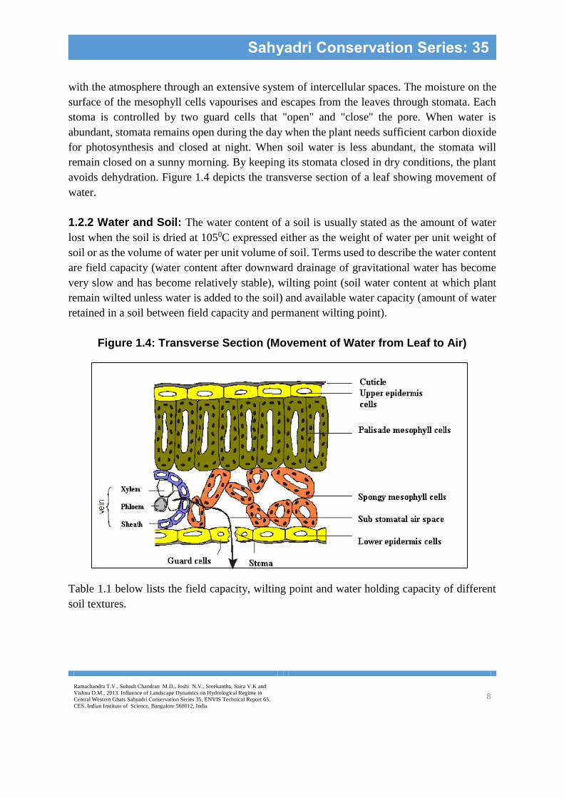
with the atmosphere through an extensive system of intercellular spaces. The moisture on the
surface of the mesophyll cells vapourises and escapes from the leaves through stomata. Each
stoma is controlled by two guard cells that "open" and "close" the pore. When water is
abundant, stomata remains open during the day when the plant needs sufficient carbon dioxide
for photosynthesis and closed at night. When soil water is less abundant, the stomata will
remain closed on a sunny morning. By keeping its stomata closed in dry conditions, the plant
avoids dehydration. Figure 1.4 depicts the transverse section of a leaf showing movement of
water.
1.2.2 Water and Soil: The water content of a soil is usually stated as the amount of water
lost when the soil is dried at 1050C expressed either as the weight of water per unit weight of
soil or as the volume of water per unit volume of soil. Terms used to describe the water content
are field capacity (water content after downward drainage of gravitational water has become
very slow and has become relatively stable), wilting point (soil water content at which plant
remain wilted unless water is added to the soil) and available water capacity (amount of water
retained in a soil between field capacity and permanent wilting point).
Figure 1.4: Transverse Section (Movement of Water from Leaf to Air)
Table 1.1 below lists the field capacity, wilting point and water holding capacity of different
soil textures.

Ramachandra T.V., Subash Chandran M.D., Joshi N.V., Sreekantha, Saira V.K and
Vishnu D.M., 2013. Influence of Landscape Dynamics on Hydrological Regime in
Central Western Ghats Sahyadri Conservation Series 35, ENVIS Technical Report 65,
CES, Indian Institute of Science, Bangalore 560012, India 9
Sahyadri Conservation Series: 35
Table 1.1: Typical Values for Soil Water Parameters by Texture
Texture class Field capacity (%) Wilting point (%) Available capacity (%)
Sand 12 4 8
Loamy sand 14 6 8
Sandy loam 23 1 13
Loam 26 12 14
Silt loam 3 15 15
Silt 32 15 17
Silt clay loam 34 19 15
Silty clay 36 21 15
Clay 36 21 15
The next section will deal with the structure of a tropical forest and an individual tree and the
important hydrological functions of each.
1.2.3 Hydrological and Other Functions of Tropical Trees: Some hydrological
characteristics of tropical trees and their hydraulic functions are discussed below:
Leaves: Compound leaves are common in tropical forests. Leaves or leaflets vary in size,
shape, texture and chemical and physiological ways. Mature leaves in the lowland forests are
generally 7-13 cm in length, somewhat elliptical in shape and of an entire, sclerophyllous type
(leathery evergreen leaves with a thick waxy cuticle to conserve water during the long, dry
summer). They become progressively smaller at higher elevations.
The leaves of the understorey trees often develop an extended drip tip or acumen, which allows
water to drain quickly from the surface. This may increase photosynthetic efficiency of the leaf
by increasing light absorption and transpiration rates, or by discouraging the growth of algae
and lichens. The leaves are smaller, more leathery in texture and have less pronounced drip tips
in the taller trees. The varying leaf types in tropical forests may result from increased water
stress in the upper canopy caused by higher insolation, stronger winds and periodic droughts.
Roots: They are important life support system for plants and thus for all life in terrestrial
ecosystems. Some of the functions of roots are given below:
Carbon pumps that feed soil organisms and contribute to soil organic matter
Storage organs
A sensor network that helps regulate plant growth
Absorptive network for limiting soil resources of water and nutrients

Ramachandra T.V., Subash Chandran M.D., Joshi N.V., Sreekantha, Saira V.K and
Vishnu D.M., 2013. Influence of Landscape Dynamics on Hydrological Regime in
Central Western Ghats Sahyadri Conservation Series 35, ENVIS Technical Report 65,
CES, Indian Institute of Science, Bangalore 560012, India 10
Sahyadri Conservation Series: 35
Mechanical structures that support plants, strengthen soil, construct channels, break
rocks, etc.
Hydraulic conduits that redistribute soil water and nutrients
Habitats for mycorrhizal fungi and rhizosphere organisms
The first root to emerge from a seed is the radicle or primary root. In most dicots, the radicle
enlarges and forms a prominent taproot. Smaller branches or lateral roots grow from the
taproot. It functions as food reserves such as carbohydrate storage or for reaching water deep
in the ground. Taproots usually control growth and development of branch roots. Taproots
grow longer than branch roots. Compared to this, most monocots have a fibrous root system
consisting of an extensive mass of similarly sized roots. In these plants, the radicle is short
lived and roots are adventitious, which means they can grow from plant organs other than roots
e.g. stems.
A tree, which has a deep and thick taproot immediately beneath the trunk, can transmit forces
directly into the ground. However, many trees have their largest roots radiating from the base
of the trunk in the upper layers of the soil, creating a shallow plate of woody roots. These
woody roots eventually form buttresses to prevent the tree from uprooting when there is wind
loading. Appendix I give the rooting depths of some tree species in Western Ghats.
Tree root systems can be divided based on diameter into two portions namely fine and coarse.
Coarse roots are generally woody and provide a mechanical and conductive service to the tree.
Water and minerals are taken up by the fine roots that separate through the mineral soil and
sometimes litter layer as well.
The effectiveness of water uptake by trees depends on the effectiveness with which soil is
exploited by roots, contact between roots and soil and the hydraulic potential gradients between
roots and soil (Landsberg and Gower, 1997). Tree root architecture varies between species and
is affected by soil type and growing conditions. From a water collection and transport point of
view, the optimum system will be a considerable root biomass, with high root length per unit
volume of soil, in the surface layers of the soil to harvest as much water as possible, with larger
more, widely spaced roots deeper in the soil. These will absorb more water slowly, but the
deeper soil layers do not dry as fast as the surface layers; therefore deep roots are likely to play
an important role in maintaining water uptake and transpiration during dry periods. Soil textural
characteristics and hard pans can greatly alter the development and vertical distribution of large
roots.
Belowground root system architecture of forests can influence patterns of soil water utilization
by trees and ultimately canopy transpiration. Deeply rooted trees and other plants can lift water
hydraulically from moist soil horizons several meters below ground to drier portions of the soil

Ramachandra T.V., Subash Chandran M.D., Joshi N.V., Sreekantha, Saira V.K and
Vishnu D.M., 2013. Influence of Landscape Dynamics on Hydrological Regime in
Central Western Ghats Sahyadri Conservation Series 35, ENVIS Technical Report 65,
CES, Indian Institute of Science, Bangalore 560012, India 11
Sahyadri Conservation Series: 35
profile where it is released into the soil (Brooks et al. 2002). The process is considered passive,
as it requires only a water potential gradient from moist soil layers through the root xylem to
dry soil layers, and a relatively low resistance to reverse flow from the roots. Although the
direction of water movement is typically upward, towards drier, shallow soil layers,
measurements of sap flow in taproots and lateral roots of trees have demonstrated that roots
can also redistribute water either downward or laterally from moist surface soils to drier regions
of soil (Burgess et al. 1998, 2001; Sakuratani et al. 1999; Smith et al. 1999). Since it can be
bidirectional and is apparently passive, “hydraulic redistribution” has been proposed as a more
comprehensive term than “hydraulic lift” to describe the phenomenon (Burgess et al. 1998).
Hydraulic redistribution usually occurs at night when transpiration has diminished sufficiently
to allow the water potential of the roots to exceed that of the drier portions of the soil profile
(Brooks et al. 2002).
The above sections dealt with a tree, which is a higher plant and its hydrological characteristics.
The next section discusses the water need of an agricultural crop.
1.2.4 Crop Water Need: The water need of a crop consists of transpiration plus evaporation.
Therefore, the crop water need is also called "evapotranspiration". When the plants are very
small evaporation will be more important than transpiration and when the plants are fully
grown, transpiration is more important than the evaporation. Table 1.2 summarises the effect
of climatic factor on crop water needs.
A certain crop grown in a sunny and hot climate needs per day more water than the same crop
grown in a cloudy and cooler climate. There are, however - apart from sunshine and
temperature - other climatic factors, which influence the crop water, need. These factors are
humidity and wind speed. When it is dry, the crop water needs are higher than when it is humid.
In windy climates, the crops will use more water than in calm climates.
Table 1.2: Effect of Major Climatic Factors on Crop Water Needs
Climatic factor Crop water need
High Low
Solar energy Sunny (no clouds) Cloudy (no sun)
Temperature Hot Cool
Humidity Dry Humid
Wind speed Windy Little wind
Table 1.3 gives the seasonal crop water needs of certain crops.

Ramachandra T.V., Subash Chandran M.D., Joshi N.V., Sreekantha, Saira V.K and
Vishnu D.M., 2013. Influence of Landscape Dynamics on Hydrological Regime in
Central Western Ghats Sahyadri Conservation Series 35, ENVIS Technical Report 65,
CES, Indian Institute of Science, Bangalore 560012, India 12
Sahyadri Conservation Series: 35
Table 1.3: Approximate Values of Seasonal Crop Water Needs
Crop Crop water need
(mm/total growing period)
Alfalfa 800-1600
Tomato 400-800
Cotton 700-1300
Potato 500-700
Pepper 600-900
Sugarcane 1500-2500
Rice (paddy) 450-700
Percolation is more in submerged rice lands. In lighter soils, such losses amount to about 60%
percent of total water requirement. Soil compaction and puddling is done to reduce these losses.
Transpiration accounts for about 40%. Evaporation depends upon the climatic factors and
range from 20-40%.
1.3 Land use/Land cover Change and its Effect on the Hydrological Cycle
Land cover is the observed physical cover at a given location and time as might be seen on the
ground or from remote sensing. This includes the vegetation (natural or planted) and human
constructions (buildings etc.), which cover the earth’s surface. Land use is, in part a description
of function, the purpose for which the land is being used. Land use and cover changes are the
result of many interacting processes. Each of these processes operate over a range of spatial,
temporal, quantitative, or analytical dimension used by scientists to measure and study objects
and processes.
Land-use and land-cover are linked to climate and weather in complex ways. Key links between
changes in land cover and climate include the exchange of greenhouse gases (such as water
vapor, carbon dioxide, methane, and nitrous oxide) between land surface and atmosphere, the
radiation (both short and longwave) balance of land surface, the exchange of sensible heat
between land surface and atmosphere, and roughness of the land surface and its uptake of
momentum from atmosphere. Artificial changes to the natural cycle of water have produced
changes in aquatic, riparian, wetland habitats and agricultural landscape. These interferences
have had both positive and negative impacts on the problems that they were intended to solve.
Some of these activities have greatly constrained the degree of interactions between the river
channel and the associated floodplain with catastrophic effects on biodiversity.
Ramachandra T.V., Subash Chandran M.D., Joshi N.V., Sreekantha, Saira V.K and
Vishnu D.M., 2013. Influence of Landscape Dynamics on Hydrological Regime in
Central Western Ghats Sahyadri Conservation Series 35, ENVIS Technical Report 65,
CES, Indian Institute of Science, Bangalore 560012, India 13
Sahyadri Conservation Series: 35
1.4 Use of Remote Sensing and GIS Techniques in Hydrology
Remote sensing uses measurements of the electromagnetic spectrum to characterize the
landscape or infer properties of it. There are 3 characteristics of remote sensing that make it a
potentially very powerful tool for advancing hydrologic sciences (Schultz and Engman, 2000).
Measuring system states- Thermal infrared and microwave remote sensing due to their
unique responses to surface properties important to hydrology, such as surface
temperature, soil moisture and snow water content, have the capability to measure
these system states directly.
Area versus point data- Use of data representing an area in which the spatial variability
of specific parameters of the area have been integrated may help provide one of the
keys to understand scaling and scale interdependence in hydrologic systems.
Temporal data- Remote sensing data from satellite platform can provide unique time
series data for hydrologic use. The actual frequency of observation can vary from
continuous to once every two weeks or so, depending upon the sensors and type of
orbit. Temporal data may provide means for imparting hydrologic interpretation to
certain observations. For example, observing the time changes in soil moisture may
provide information on soil types and even hydraulic properties such as hydraulic
conductivity.
A major focus of remote sensing research in hydrology has been to develop approaches for
estimating hydro-meteorological states and fluxes. The primary set of state variables include
land surface temperature, near surface soil moisture, snow cover/water equivalent, water
quality, water quantity, landscape roughness, land use and vegetation cover (Schmugge at al.,
2002). The hydrometerological fluxes are primarily soil evaporation and plant transpiration or
evapotranspiration and snow melt runoff.
Remote sensing data has been used to understand the vegetation dynamics, which are acquired
by sensors on various remote platforms, such as multi spectral and thermal scanners and active
microwave (radar) imaging systems. Since satellite observations are available since the early
1970s, it is possible to relate trends such as vegetation cover densities to stream flow.
The land cover maps derived by remote sensing are the basis of hydrologic response units for
modelling. Effective utilization of spatial data involves the existence of an efficient, geographic
handling and processing system that can transform the data into usable information. A major
tool for handling spatial data is geographic information system (GIS). Data analysis and spatial
modeling capability are the most important characteristics of a GIS (Schultz and Engman,
2000).

Ramachandra T.V., Subash Chandran M.D., Joshi N.V., Sreekantha, Saira V.K and
Vishnu D.M., 2013. Influence of Landscape Dynamics on Hydrological Regime in
Central Western Ghats Sahyadri Conservation Series 35, ENVIS Technical Report 65,
CES, Indian Institute of Science, Bangalore 560012, India 14
Sahyadri Conservation Series: 35
Geographic information systems deal with information about features that is referenced by a
geographical location. These systems are capable of handling both locational data and attribute
data about such features through database management system (DBMS). Geographic
information systems are useful in hydrological studies as it allows the integration of a
combination of spatial data such as soil, topography, hydrologic variables such as soil moisture.
1.5 Objectives
The objectives of the study are:
i). Quantification of hydrologic components of Sharavathi River Basin, Western Ghats using
Remote Sensing and GIS.
ii). Study the effect of land use/land cover changes on hydrologic components.
Significance of the Study
The Western Ghats comprise the mountain range that runs along the western coast of India,
from the Vindhya-Satpura ranges in the north to the southern tip. This range intercepts the
moisture laden winds of the southwest monsoon thereby determining the climate and
vegetation of the southern peninsula. The steep gradients of altitude, aspect and rainfall make
the region ecologically rich in flora and fauna.
There is a great variety of vegetation all along the Ghats: scrub jungles, grassland along the
lower altitudes, dry and moist deciduous forests, and semi-evergreen and evergreen forests.
Out of the 13,500 species of flowering plants in India, 4500 are found in the Western Ghats
and of these 742 are found in Sharavathi river basin (Ramachandra et al. 2007). Climax
vegetation of the wet tract consists of Cullenia, Persea, Diptercarpus, Diospyros and
Memecylon. The deciduous forest tract is dominated by Terminalia, Lagerstroemia, Xylia,
Tectona and Anogeissus. The region also contains potentially valuable spices and fruits such
as wild pepper varieties, cardamom, mango, jackfruit and other widely cultivated plants. There
is an equal diversity of animal and bird life. Noticeable reptile fauna in the evergreen forests
include burrowing snakes (uropeltids) (Gadgil & Meher-Homji, 1990) and the king cobra and
among amphibians, the limbless frog (caecilians). The Nilgiri langur, lion-tailed macaque,
Nilgiri tahr and Malabar large spotted civet are some examples of endangered endemic
mammals belonging to this area.
Sharavathi river valley lies in the Central Western Ghats and represents an area of 2985 km2.
Sharavathi is a west flowing river originating at Ambuthirtha in Shimoga district and during
its course, falls from a height of around 253 m at the famed Jog Falls. It flows through Honnavar
and eventually into the Arabian Sea.

Ramachandra T.V., Subash Chandran M.D., Joshi N.V., Sreekantha, Saira V.K and
Vishnu D.M., 2013. Influence of Landscape Dynamics on Hydrological Regime in
Central Western Ghats Sahyadri Conservation Series 35, ENVIS Technical Report 65,
CES, Indian Institute of Science, Bangalore 560012, India 15
Sahyadri Conservation Series: 35
Karnataka Power Cooperation (KPCL) set up a dam across Sharavathi in 1964 known as
Linganamakki Dam to harness electricity, which has divided the river basin into upstream and
downstream. The construction of this dam has made considerable hydrological and ecological
alterations in the river basin. The dam resulted in the submergence of wetlands and forest areas
of unmeasured biodiversity. The effects are particularly seen in the upstream of the river basin
where the dam submerged many villages and forests to give rise to small isolated islands. These
island and surrounding areas have created niches for 150 species of birds, 145 species of
butterflies and 180 species of beetles along with mammals such as spotted deer, barking deer,
civet, leopard and the Indian gaur.
The reservoir has provided further impetus to farmers and plantation agriculturists. Large tracts
of forestlands have been cleared for paddy cultivation and plantation trees such as areca and
acacia. Apart from these, vast tracts of natural vegetation has been cleared and replaced with
monoculture plantations of Acacia auriculiformis, Eucalyptus sp. and Tectona grandis. As a
result of these activities, there is evidence of changes in runoff and stream flow regimes. There
are instances where wells have ‘run dry’ in the wet spots of the basin, mainly because
percolation of rainwater into the ground has decreased due to deforestation. Studies are thus
required to quantify the hydrological responses in order to gain an understanding of the effect
of anthropogenic activities on the hydrological components and thus the vegetation of study
area.
Ramachandra T.V., Subash Chandran M.D., Joshi N.V., Sreekantha, Saira V.K and
Vishnu D.M., 2013. Influence of Landscape Dynamics on Hydrological Regime in
Central Western Ghats Sahyadri Conservation Series 35, ENVIS Technical Report 65,
CES, Indian Institute of Science, Bangalore 560012, India 16
Sahyadri Conservation Series: 35
2.0 Review of Literature
This section presents a review of the major components in the hydrological cycle along with
their conventional and remote sensing measurement techniques.
Precipitation: It is the principal component of the hydrological cycle, and as such is of
primary importance in hydrology. The form and quantity of precipitation are influenced by
static and dynamic factors. Static influences are those that do not vary between storm events
such as aspect and slope (Davie, 2003). The influence of aspect plays an important part in the
distribution of precipitation throughout a catchment (Davie, 2003). Aspect refers to the
direction in which the slope of a mountain faces. In Western Ghats, the predominant source of
rainfall is through monsoons arriving from the west. Slopes with aspects facing away from the
predominant weather patterns will receive less rainfall than their opposites. The influence of
slope is only relevant at a very small scale. Dynamic influences are those that changes and are
caused by the variation in the weather and the variation and type of vegetation. Weather
patterns influence precipitation especially on a global scale. Solar energy is the primary driver
for weather. Consequently, all motion in the atmosphere and ocean is a result of distribution of
heating and cooling around the earth. Monsoon rain and winds are the result of such heating
patterns. Another important dynamic influence is vegetation such as forests. Forests create
additional roughness for air masses moving in the lower atmosphere, slows down their
movement and causes turbulence, which leads to the formation of ascending air fluxes, air
cooling, cloud formation, and, consequently, greater precipitation on forested areas.
Western Ghats experience two main rainfall seasons. They are:
South-west monsoon (June-September)
North east monsoon (October-November)
The Western Ghats is considered an important barrier for the Arabian Sea branch of the
monsoon. The moist air currents, which approach the Western Ghats are forced to ascend the
mountains. In this process, they shed their moisture in the form of frequent and heavy rains
over the Ghats. After ascending, the monsoon winds advance into the Deccan plateau and
beyond.
Western Ghats region experiences heavy rainfall but studies have proved that monsoons may
not be the only one responsible for it. A westerly stream of air, such as the monsoon does not
have sufficient energy to climb the Ghats unless fed by another source. Investigation by Sarkar,
(1979) suggests that the Western Ghats may be responsible for about 60% of the observed
rainfall and, on rare occasions, even 80%, by forcing the monsoon air to ascend. The peak
Ramachandra T.V., Subash Chandran M.D., Joshi N.V., Sreekantha, Saira V.K and
Vishnu D.M., 2013. Influence of Landscape Dynamics on Hydrological Regime in
Central Western Ghats Sahyadri Conservation Series 35, ENVIS Technical Report 65,
CES, Indian Institute of Science, Bangalore 560012, India 17
Sahyadri Conservation Series: 35
rainfall occurs on the windward side at a distance of 10 to 12 km from the crest of the Western
Ghats. Thus, high rainfalls in the Western Ghats can be attributed to a secondary source of
moisture. If this is the case, then the forest cover on this mountain range could have a major
role in generating humidity in the air.
Precipitation is one of the most challenging variables to quantify due to its extreme transience
and spatial heterogeneity. Remote sensing techniques have made advances in quantifying
precipitation using different bands viz. visible and microwave. The following section will
review the conventional and remote sensing techniques in estimating rainfall.
Some of the conventional techniques are given in Table 2.1
Table 2.1: Conventional Techniques in Measuring Rainfall
Type of measurement Method References
Point measurement Rain gauge Mutreja, 1986
Areal measurement Arithmetic mean Mutreja, 1986
Thiessen’s polygon Mutreja, 1986
Isohyetal Mutreja, 1986
Hypsometric Davie, 2003
Weather radar Collier, 2000
In India, the installation and observation of rain gauges throughout the country are controlled
by the Indian Meteorological Department and a standard rain gauge called the Symon’s gauge
is used at almost all the places. Rainfall is measured by either non-recording gauges or
recording gauges and 3) weather radars.
Areal measurement of precipitation includes arithmetic average, Thiessen’s polygon, isohyetal
and hypsometric method. Arithmetic mean method is used if the gauges are uniformly
distributed and the topography, flat (Mutreja, 1986). Disadvantages of this method are that it
gives poor results when gauges are relatively few and requires a denser network of gauges.
Raingauges outside the boundary of the watershed should not be used for arithmetic averaging
(Singh, 1992). Thiessen’s method attempts to define the area represented by each gauge in
order to weigh the effects of non uniform rainfall distribution (Singh, 1992). Thiessen’s method
is usually more accurate than arithmetic average and gives consistent results when storm means
are computed by different people. However, this method has the disadvantage of not accounting
for orographic influences and also station weights have to be re-determined whenever rain
gauge networks changes. Isohyetal method is generally considered the most accurate method
for computing average rainfall over a drainage basin. In this method, topographic influences
have been taken into account and the stations outside the basin can also be used. Nevertheless,

Ramachandra T.V., Subash Chandran M.D., Joshi N.V., Sreekantha, Saira V.K and
Vishnu D.M., 2013. Influence of Landscape Dynamics on Hydrological Regime in
Central Western Ghats Sahyadri Conservation Series 35, ENVIS Technical Report 65,
CES, Indian Institute of Science, Bangalore 560012, India 18
Sahyadri Conservation Series: 35
it is a laborious method and different persons may obtain varying results from the same data.
Hypsometric method assumes that the relationship between altitude and rainfall is linear, which
is not always the case and warrants exploration before using the technique (Davie, 2003).
Ground based radar offers areal measurements of precipitation from a single location over a
large area in near real-time. Both single and mutlipolarisation radars have been used over a
range of wavelengths (Collier, 2000). While weather radar does offer a means of making wide
area measurements over specific important land and coastal areas, it does not offer a practical
method of making measurements over large remote river catchments or oceans. The use of
satellite has been investigated to compensate for these difficulties. Meteorological satellites
now provide a realistic means to monitor the spatial and temporal distributions of precipitation.
Table 2.2 below lists some of the platforms and sensors commonly used to estimate
precipitation overland.
Table 2.2: Operational Sensors to Measure Precipitation
Platform Sensors Orbit Resolution
GOES-7
GOES-8
GOES-9
VISSR
GOES I-M imager
GOES I-M imager
Geostationary 1 km (VIS) and 4
km (IR)
Meteosat-5 Meteosat imager Geostationary 2.5 km(VIS) and 5
km (IR)
NOAA-12,14 AVHRR Sun synchronous 1.1 km (VIS/IR)
DMSP F-10,11,13 SSM/I Sun synchronous 15 km
There is a large number of satellite estimation algorithms documented in literature. For
example, 55 algorithms were evaluated in the Third Algorithm Intercomparison Project (AIP-
3) of the Global Precipitation Climatology Project (GPCP), including 16 using visible and infra
red images, 29 using microwave images and 10 using mixed infrared/microwave images. Table
2.3 gives the estimation methods using visible/infrared and microwave bands. Visible/infrared
techniques derive qualitative or quantitative techniques estimates of rainfall from satellite
imagery through indirect relationships between solar radiance reflected by clouds (cloud
brightness temperatures) and precipitation (Collier, 2000). However, relationships derived
using life history and cloud indexing techniques for a given region and a given time period may
not be valid for a different location and/or season. Other problems include difficulties in
defining rain/no rain boundaries and inability to cope with rainfall patterns at the meso or local
scales. RAINSAT is a supervised classification algorithm, which is trained to identify areas of
precipitation from a combination of visible and infrared imagery. The advantage of this method
is that at night since visible imagery is unavailable it can revert to a pure infrared technique.
Ramachandra T.V., Subash Chandran M.D., Joshi N.V., Sreekantha, Saira V.K and
Vishnu D.M., 2013. Influence of Landscape Dynamics on Hydrological Regime in
Central Western Ghats Sahyadri Conservation Series 35, ENVIS Technical Report 65,
CES, Indian Institute of Science, Bangalore 560012, India 19
Sahyadri Conservation Series: 35
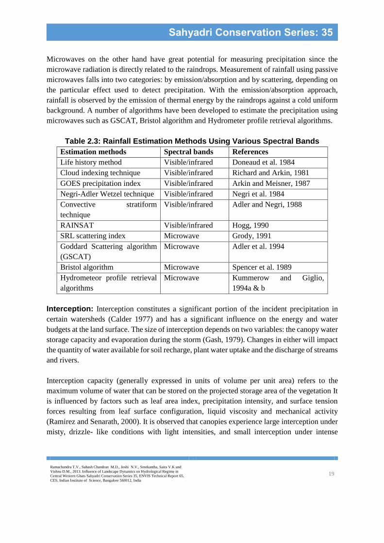
Microwaves on the other hand have great potential for measuring precipitation since the
microwave radiation is directly related to the raindrops. Measurement of rainfall using passive
microwaves falls into two categories: by emission/absorption and by scattering, depending on
the particular effect used to detect precipitation. With the emission/absorption approach,
rainfall is observed by the emission of thermal energy by the raindrops against a cold uniform
background. A number of algorithms have been developed to estimate the precipitation using
microwaves such as GSCAT, Bristol algorithm and Hydrometer profile retrieval algorithms.
Table 2.3: Rainfall Estimation Methods Using Various Spectral Bands
Estimation methods Spectral bands References
Life history method Visible/infrared Doneaud et al. 1984
Cloud indexing technique Visible/infrared Richard and Arkin, 1981
GOES precipitation index Visible/infrared Arkin and Meisner, 1987
Negri-Adler Wetzel technique Visible/infrared Negri et al. 1984
Convective stratiform
technique
Visible/infrared Adler and Negri, 1988
RAINSAT Visible/infrared Hogg, 1990
SRL scattering index Microwave Grody, 1991
Goddard Scattering algorithm
(GSCAT)
Microwave Adler et al. 1994
Bristol algorithm Microwave Spencer et al. 1989
Hydrometeor profile retrieval
algorithms
Microwave Kummerow and Giglio,
1994a & b
Interception: Interception constitutes a significant portion of the incident precipitation in
certain watersheds (Calder 1977) and has a significant influence on the energy and water
budgets at the land surface. The size of interception depends on two variables: the canopy water
storage capacity and evaporation during the storm (Gash, 1979). Changes in either will impact
the quantity of water available for soil recharge, plant water uptake and the discharge of streams
and rivers.
Interception capacity (generally expressed in units of volume per unit area) refers to the
maximum volume of water that can be stored on the projected storage area of the vegetation It
is influenced by factors such as leaf area index, precipitation intensity, and surface tension
forces resulting from leaf surface configuration, liquid viscosity and mechanical activity
(Ramirez and Senarath, 2000). It is observed that canopies experience large interception under
misty, drizzle- like conditions with light intensities, and small interception under intense
Ramachandra T.V., Subash Chandran M.D., Joshi N.V., Sreekantha, Saira V.K and
Vishnu D.M., 2013. Influence of Landscape Dynamics on Hydrological Regime in
Central Western Ghats Sahyadri Conservation Series 35, ENVIS Technical Report 65,
CES, Indian Institute of Science, Bangalore 560012, India 20
Sahyadri Conservation Series: 35
precipitation conditions. Rainfall interception loss accounts for 10 to 40% of rainfall entering
a forest canopy (Zinke, 1967).
The following discussion on interception by different kind of forests has been adapted from
Crockford and Richardson (2000).
Valente et al. (1997) studied interception of a Pinus pinaster plantation and a Eucalyptus
globulus plantation in Portugal, with an annual rainfall of 800 mm. Interception values were
17.1% and 10.8% of gross rainfall for the pines and eucalyptus respectively. The
interception/LAI ratio for the pines is 6.3 compared with 3.4 for the eucalypt forest, i.e. on a
per LAI basis the pine needles intercepted almost twice as much rainfall as the eucalypt leaves.
This could be due to the pine needle clusters being able to hold intercepted rainfall more
securely than the vertically aligned eucalypt leaves.
Asdak et al. 1998 in a study of rainfall interception in a tropical rainforest (annual rainfall of
errors in the estimation of throughfall. It is also seen that interception from rainforest is much
higher than temperate forests due to the large intercepting surfaces (leaf and wood).
In an undisturbed Amazon rainforest Lloyd et al. (1988) found interception to be 8.9% of gross
rainfall, from 625 days of data. Rainfall for this period was 4804 mm. Stemflow was 1.8% of
rainfall.
In a study of two tropical montane rainforests, at different elevations, in Columbia (Veneklaas
and Van Ek, 1990), it was found that the forest at higher elevation (3370 m) had higher
interception loss than the forest at lower elevation (2115 m). The values were 18.2 and 12.4%
respectively. The site at higher elevation site had fewer trees than site at lower elevation site,
but were larger. It was stated that the upper canopy at lower elevation was more open than at
higher elevation, but total crown cover was greater in the former owing to the presence of
smaller sized trees. Herbs and shrubs also dominated the understorey in the low elevation
forests. Rainfall at the higher elevation site was less than the low elevation site as well as being
of lower intensity and longer duration. This combination of factors would favour greater
interception in the forests at higher elevation site. Also, the epiphyte population was greater at
this site. As the epiphytes were concentrated in the upper parts of the trees they could enhance
interception.
Bruijnzeel and Wiersum, 1987 studied rainfall interception in Acacia auriculiformis in West
Java, Indonesia and found increase in interception from year 1 (11.2%) and year 2 (17.9%).
The reason attributed to this was an increase in biomass- about 20% for basal area and leaf area
index (LAI). Stemflow decreased from 7.9% in year 1 to 6.2% in year 2. Thus, change in plant

Ramachandra T.V., Subash Chandran M.D., Joshi N.V., Sreekantha, Saira V.K and
Vishnu D.M., 2013. Influence of Landscape Dynamics on Hydrological Regime in
Central Western Ghats Sahyadri Conservation Series 35, ENVIS Technical Report 65,
CES, Indian Institute of Science, Bangalore 560012, India 21
Sahyadri Conservation Series: 35
structure such as growth of second order branches particularly on the lower side can increase
interception. Some techniques for measuring interception are given below.
Knowledge about the interception processes was first formulised by Horton, (1919). It was a
semi-empirical model of rainfall interception, constructed by plotting precipitation against
throughfall. Horton’s model is considered to be the simplest empirical approach to model
interception. Another variant of Horton’s model describes interception as a function of canopy
storage capacity, evaporative fraction and rainfall (Singh, 1992). It is commonly used in areas
where rainfall is high and has been adopted to calculate interception from different kinds of
vegetation in the study area. Horton (1919) describes interception as a function of canopy
storage capacity C and evaporative fraction () and is given by the equation
PCI (2.1)
Putty and Prasad (2000) have suggested the following canopy storage capacities for Western
Ghats.
Table 2.4: C Values for Different Vegetation Types in Western Ghats
Land use Canopy storage capacity (mm)
Evergreen forest (dense) 4.5-5.5
Deciduous/open forests (plantations) 4-5
Scrub 2.5-3.5
Grass 1.8-2.0
Paddy (valley) 1.8-2
In the classical model of Rutter et al, (1971), canopy was considered to be a single
compartment filled by rain and emptied by evaporation and drainage. The canopy water
balance was calculated with a time step of one hour. This direct throughfall fraction was
assumed to be proportional to the fractional canopy cover (Aston, 1979). The drainage rate was
an exponential function of the amount of storage in the canopy. The evaporation rate was
calculated from atmospheric data according to Penman (1948).
Other complicated models based on Rutter simulate the atmospheric transport within the
horizontal layers of the canopy and calculate the atmospheric transport between these layers.
The drainage rate has been set proportional to the rainfall intensity. A recent model considered
individual leaves in the canopy as tipping buckets: when the total force, acting on the leaf
surface as a result of both the water stored and the raindrop hitting the leaf, was greater than a
certain factor, the leaf tipped, and the water storage on the leaf was reduced to a minimum

Ramachandra T.V., Subash Chandran M.D., Joshi N.V., Sreekantha, Saira V.K and
Vishnu D.M., 2013. Influence of Landscape Dynamics on Hydrological Regime in
Central Western Ghats Sahyadri Conservation Series 35, ENVIS Technical Report 65,
CES, Indian Institute of Science, Bangalore 560012, India 22
Sahyadri Conservation Series: 35
storage. The leaves were ordered in horizontal layers that could be hit by rain with a horizontal
component (Xiao et al., 2000).
Interception can also be considered as the function of aboveground biomass (Savabi and Stott,
1994)
I = 0.001(3.7 VE –(1.1 x 10⁻⁴ VE2))
Where, VE –above ground biomass in kg/m2
Field measurements have been carried out to determine throughfall and stemflow. Throughfall
is variable in most forests and its accurate estimation is quite difficult. It has been measured
with a range of devices, from troughs of various sizes, to plastic funnels and standard rain
gauges. For collection of stemflow, Crockford and Richardson (1990b) suggests the use of
split plastic hose, internal diameter =14mm. It was wrapped around the tree and attached with
galvanized iron staples then sealed with neutral silicone sealant.
In current global circulation models land surfaces schemes, interception is described as a
function of seasonal leaf area index (LAI) and fractional vegetation cover (Sellers et al. 1986).
Viessman et al., 1989 considers interception as a function of leaf area index
I= C + LAI x E x t
where, I – interception; C-canopy storage capacity in mm; LAI –leaf area index;
E – evaporation in mm; t-duration of rainfall in hours
Surface Runoff: It occurs when precipitation moves across the land surface-some of which
eventually reaches natural or artificial systems and lakes. Runoff is an important process at the
basin or watershed scale, since it can recharge reservoirs and replenish rivers that may
subsequently recharge the groundwater. It can also cause erosion and excess runoff that can
lead to flooding. Runoff is one of the most important hydrologic variables used in most of the
water resources applications. Conventional models for prediction of river discharge require
considerable hydrological and meteorological data. Collection of these data is expensive, time
consuming and a difficult process.
Robert Horton in the 1930s suggested that storm runoff is often purely surface runoff or
overland flow (Hortonian overland flow). Horton put forward the theory that the soil surface
acted as a separating surface between surface runoff and subsurface runoff (interflow).
However, further studies revealed that this is not often the case and a watershed cannot
experience overland flow in the entire area. Hewlett and Hibbert (1967) suggested another
mechanism for the occurrence of overland flow. They hypothesised that during a rainfall event
all the water infiltrated the surface. Due to a mixture of infiltration and percolation, the water
table would rise until in some places it reached the surface. At this stage, overland flow will
occur as a mixture of return flow (i.e. water that has been beneath the ground but returns to the

Ramachandra T.V., Subash Chandran M.D., Joshi N.V., Sreekantha, Saira V.K and
Vishnu D.M., 2013. Influence of Landscape Dynamics on Hydrological Regime in
Central Western Ghats Sahyadri Conservation Series 35, ENVIS Technical Report 65,
CES, Indian Institute of Science, Bangalore 560012, India 23
Sahyadri Conservation Series: 35
surface) and rainfall falling on saturated areas. This type of overland flow is called saturated
overland flow and occurs in places where the water table is closest to the surface. The saturated
areas immediately adjacent to a stream acted as extended channel networks. This is referred to
as the variable source area concept.
Another concept called the partial areas concept states that the entire area within the watershed
may not contribute to runoff (Viessman et al., 1989). Precipitation falling on or flowing into
depressed or blocked areas can exit only by seepage or evaporation or by transpiration if
vegetated. If sufficient rainfall occurs, such areas may overflow and contribute to runoff. Thus,
the total area contributing to runoff varies with the intensity and duration of the storm.
Studies in river basins have proved that the processes suggested by Horton and Hewlett and
Hibbert hold good. It is also accepted that saturated overland flow is the dominant overland
flow occurring in humid midlatitudes and the variable source area concept is considered the
most valid when describing storm runoff (Davie, 2003). However, where the infiltration
capacity of a soil is low or the rainfall rates are high, Hortonian overland flow occurs. Examples
of low infiltration soil include, compacted soil, pavements, roads and hydrophobic soils.
Many methods for estimating runoff exist. Runoff volume or rate estimation involves
estimating the amount of rainfall exceeding infiltration and initial abstractions, which must be
satisfied before the occurrence of runoff. Infiltration excess runoff can be estimated using
different techniques. Conventional and remote sensing techniques are discussed below. Some
conventional techniques for estimation of runoff are as follows:
Table 2.5: Conventional Methods in Estimating Runoff
Methods References
Empirical formulae, curves and tables Raghunath, 1985
Rational method Raghunath, 1985
Unit hydrograph Singh, 1992
Geomorphologic instantaneous unit
hydrograph (GIUH)
Rodriguez-Iturbe and Valdes (1979)
Geomorphology-based artificial neural
network (GANN)
Zhang and Govindaraju (2003)
Several formulae, curves and tables have been developed. The usual form of the equation is
either R = aP+b or R = aPn. However, these equations are empirical and derived values are
applicable only when the rainfall characteristics and the initial soil moisture conditions are
identical to those for which these are derived. Another common method of runoff estimation is
Ramachandra T.V., Subash Chandran M.D., Joshi N.V., Sreekantha, Saira V.K and
Vishnu D.M., 2013. Influence of Landscape Dynamics on Hydrological Regime in
Central Western Ghats Sahyadri Conservation Series 35, ENVIS Technical Report 65,
CES, Indian Institute of Science, Bangalore 560012, India 24
Sahyadri Conservation Series: 35
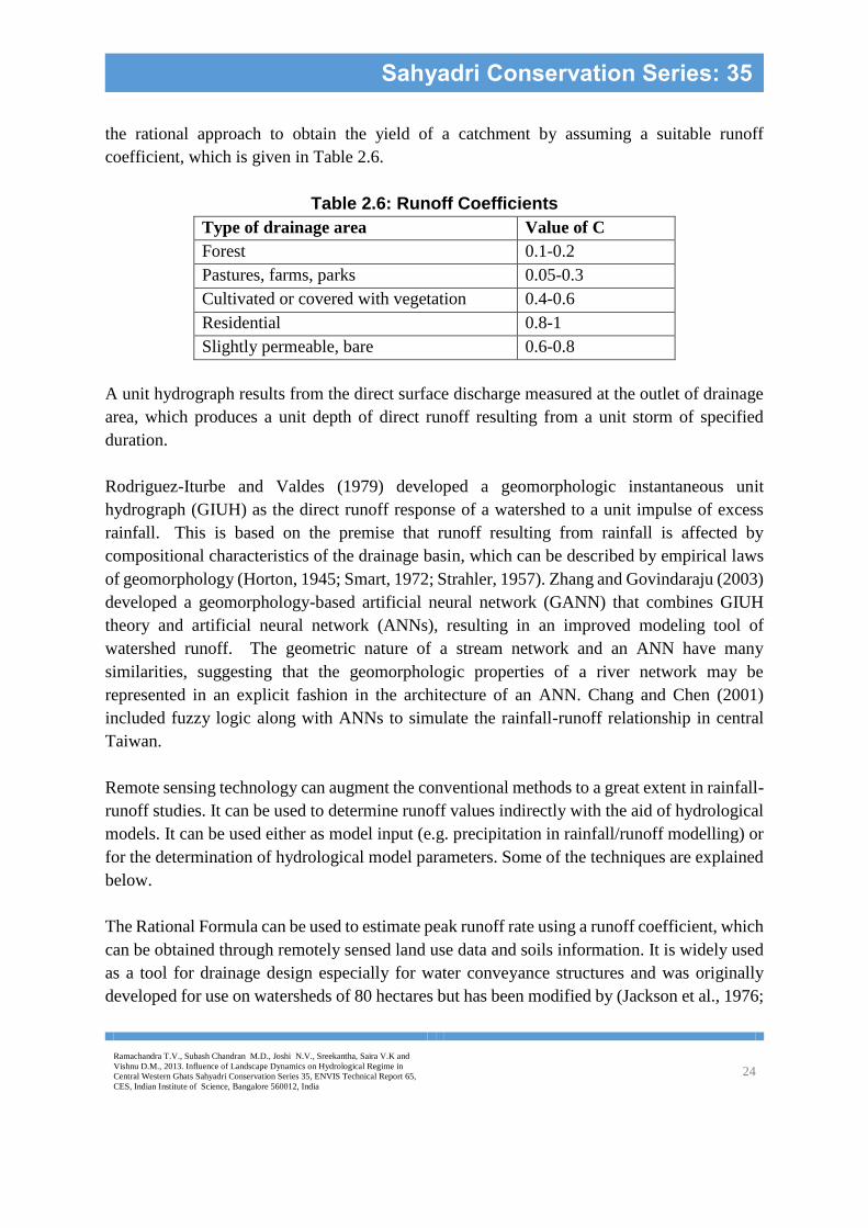
the rational approach to obtain the yield of a catchment by assuming a suitable runoff
coefficient, which is given in Table 2.6.
Table 2.6: Runoff Coefficients
Type of drainage area Value of C
Forest 0.1-0.2
Pastures, farms, parks 0.05-0.3
Cultivated or covered with vegetation 0.4-0.6
Residential 0.8-1
Slightly permeable, bare 0.6-0.8
A unit hydrograph results from the direct surface discharge measured at the outlet of drainage
area, which produces a unit depth of direct runoff resulting from a unit storm of specified
duration.
Rodriguez-Iturbe and Valdes (1979) developed a geomorphologic instantaneous unit
hydrograph (GIUH) as the direct runoff response of a watershed to a unit impulse of excess
rainfall. This is based on the premise that runoff resulting from rainfall is affected by
compositional characteristics of the drainage basin, which can be described by empirical laws
of geomorphology (Horton, 1945; Smart, 1972; Strahler, 1957). Zhang and Govindaraju (2003)
developed a geomorphology-based artificial neural network (GANN) that combines GIUH
theory and artificial neural network (ANNs), resulting in an improved modeling tool of
watershed runoff. The geometric nature of a stream network and an ANN have many
similarities, suggesting that the geomorphologic properties of a river network may be
represented in an explicit fashion in the architecture of an ANN. Chang and Chen (2001)
included fuzzy logic along with ANNs to simulate the rainfall-runoff relationship in central
Taiwan.
Remote sensing technology can augment the conventional methods to a great extent in rainfall-
runoff studies. It can be used to determine runoff values indirectly with the aid of hydrological
models. It can be used either as model input (e.g. precipitation in rainfall/runoff modelling) or
for the determination of hydrological model parameters. Some of the techniques are explained
below.
The Rational Formula can be used to estimate peak runoff rate using a runoff coefficient, which
can be obtained through remotely sensed land use data and soils information. It is widely used
as a tool for drainage design especially for water conveyance structures and was originally
developed for use on watersheds of 80 hectares but has been modified by (Jackson et al., 1976;

Ramachandra T.V., Subash Chandran M.D., Joshi N.V., Sreekantha, Saira V.K and
Vishnu D.M., 2013. Influence of Landscape Dynamics on Hydrological Regime in
Central Western Ghats Sahyadri Conservation Series 35, ENVIS Technical Report 65,
CES, Indian Institute of Science, Bangalore 560012, India 25
Sahyadri Conservation Series: 35
Still and Shih, 1985; 1991) for application to larger watersheds, principally by land-cover based
area weighting of coefficients.
The USDA Natural Resources Conservation Service-Curve Number (NRCS-CN) combines
remotely sensed land use data and soil information to determine soil's abstraction. This method
for estimating direct runoff volume has become widely used as a tool for drainage design,
particularly for impoundment structures on ungauged watersheds. Although originally
designed for use on watersheds of 1,500 ha, it has been modified by some users e.g. Jackson et
al., (1976) for application to larger watersheds, principally by land-cover based area weighting
of curve numbers.
Other types of runoff models that are not based on land use have been developed such as runoff
regression model based on cloud indexing technique. Cloud area and temperature are the
satellite variables used to develop a temperature weighted cloud cover index (Schultz and
Engman, 2000). This index is then transformed linearly to mean monthly runoff. Rott et al.
(1986) also developed a daily runoff model using Meteosat data for a cloud cover index.
Sub Surface Runoff: Field observations in the Western Ghats have shown that in the upper
reaches of streams, a significant contribution to runoff is by sub surface flow or pipe flow
(called Jala in Kannada). Pipes have been found in several continents and climatic conditions.
It occurs in sizes ranging from a few centimeters to more than 20 m. They are commonly but
largely erroneously thought to result from the activity of burrowing animals or decay of plant
roots, but can also form by subsurface erosion, starting with seepage erosion at the outlet and
working backward or erosion of existing macropores and desiccation cracks apart from
solution. Study of pipe flow hydrology is hampered by difficulties in measurement and tracing
pipe networks. Some pipes can be perennial and others ephemeral.
In the Western Ghats area, valley regions are covered with dense evergreen forests and
mountain tops with grass overlain by deep soil. The pipe outlets are near the valley bottoms
and the high density of forest vegetation makes it difficult for further exploration. However,
models have been developed to take into account varying source area and pipe flow, when
applied to large streams in the Western Ghats and suggest that pipe flow contribution to even
quick flow during storm periods is significant (Putty and Prasad, 1992; 1994b).
Evapotranspiration: The importance of evapotranspiration within the hydrological cycle
depends very much on the amount of water present and the available energy. Available water
supply can be from water directly on the surface in a lake, river or pond. In this case, it is open
water evaporation. When the water is present in the soil, the water supply becomes more
complex (Davie, 2003). As the water is removed from the soil surface and vegetation, it sets
Ramachandra T.V., Subash Chandran M.D., Joshi N.V., Sreekantha, Saira V.K and
Vishnu D.M., 2013. Influence of Landscape Dynamics on Hydrological Regime in
Central Western Ghats Sahyadri Conservation Series 35, ENVIS Technical Report 65,
CES, Indian Institute of Science, Bangalore 560012, India 26
Sahyadri Conservation Series: 35
up a moisture gradient that will draw water from deeper in the soil towards the surface, but it
must overcome the force of gravity and the withholding force exerted by the soil capillaries.
In the absence of restrictions due to water availability at the evaporative surface, the amount of
radiant energy captured at the earth’s surface is the dominant control on regional evaporation
rates. The energy available for evaporation, or the energy used in evaporation is balanced by
energy from several sources such as solar radiation, sensible heat and soil heat.
Surface albedo (i.e. the proportion of radiation reflected from a surface) is of major importance
in determining the absorption of solar energy. Generally albedo decreases for a given
vegetation type as the height of the vegetation increases because of internal reflections. Albedo
also decreases generally for soil and vegetation as the surface wetness increases (http://www.
unu.edu/unupress/unupbooks/80635e/80635E0n.htm). Albedo is the least for evergreen forests
and increases in moist deciduous forests, plantations and grasslands/crops.
Charney et al. (1977) have emphasized the role of lower albedo in increasing rainfall in a
forested region. Albedo is one of the factors that govern the energy balance of a surface and
therefore the rate of evapotranspiration. The total energy (i.e the sum of sensible heat, latent
heat and potential energy) imparted to the lower layers of the atmosphere increases as the
albedo decreases. The albedo of deserts or dry bare soil is much greater than that of vegetated
or forested surfaces, so the net energy imparted to the atmosphere over deserts is less in contrast
to a vegetated region where net radiation is converted into both sensible and latent heat. Thus,
the air may be cooler over a vegetated region, but its total energy content may be even greater
than air over a desert. Eventually, the water evaporated from vegetated region condenses and
fall as rain and the released latent heat warms the atmosphere. Therefore, a decrease in albedo
causes a slight decrease in large-scale atmospheric temperatures. The more complex the
vegetation structure, the greater the trapping of radiation by multiple reflection between leaves
and lower the albedo. An increase in albedo reduces the absorption of solar radiation by the
ground; consequently, there is less transfer of sensible and latent heat from the ground to the
atmosphere. In addition, the intensity of cloud cover diminishes as does the longwave flux from
the clouds to the surface of the earth, so that the net absorption at the ground (short and
longwave) is decreased. Thus, regions with increased albedo become sinks of energy and the
general motion of the atmosphere above such regions is downward. An essential prerequisite
for precipitation is upward motion, thus Charney's model provides a basis for deforestation
leading to a decrease in rainfall.
(http://www. unu.edu/unupress/unupbooks/80635e/80635E0n.htm).
Transpiration is essentially the same as evaporation except that the surface from which the
water molecules escape is not a free water surface (Veihmeyer, 1964). The surface for

Ramachandra T.V., Subash Chandran M.D., Joshi N.V., Sreekantha, Saira V.K and
Vishnu D.M., 2013. Influence of Landscape Dynamics on Hydrological Regime in
Central Western Ghats Sahyadri Conservation Series 35, ENVIS Technical Report 65,
CES, Indian Institute of Science, Bangalore 560012, India 27
Sahyadri Conservation Series: 35
transpiration is largely in leaves. Some typical canopy transpiration of different vegetation
types are given in Table 2.7.
Table 2.7: Canopy Transpiration of Different Vegetation
Vegetation Canopy transpiration in mm
Per year or per growing season Per day
Tropical tree plantations 1000-1500 2.5-4
Tropical rainforests of the
lowlands
900-2000 2.5-4
Tropical montane forests 500-850 2.5-4
Eucalyptus stands 700-800 6-7
Deciduous forests of the
temperate zone
300-600 2.5-4.5
Prairies and savannas 400-500 4-6
Meadows and pasture 250-400 4-6
Source: Larcher, 2003
Water for evapotranspiration from land is supplied mainly by the soil, and in relatively mesic
systems, most water leaves the soil through plant roots and out of plant canopies, rather than
by direct evaporation at the soil surface (Chahine 1992).
Plant root systems show a remarkable ability to adapt to soil depth and to changes in availability
of water and nutrients and the chemical properties (e.g., salinity) in soils. Plant roots transfer
water between soil layers of different water potential thereby significantly affecting the
distribution and availability of water in the soil profile (Burgess et al., 1998). The availability
of water to individual plants depends in part on local climatic and edaphic factors and also on
the depth, lateral spread and degree of overlap of plant root systems. Actual water use also
depends on plant vascular architecture and on the balance of above- and below-ground plant
dimensions (West et al. 1999). The zone of influence of trees is generally related to the extent
of their root growth. The lateral spread of roots is typically 2 to 4 times the height of the tree.
For most tree species, 80% of roots are found in the upper 30 cm of soil. Most of the remaining
20% of roots are typically found within the top 1.0 to 1.5 metres of soil, with some growing to
2.0 metres, and less frequently to as deep as 3.0 metres. In clay soils, root penetration is difficult
and the percentage of roots in the upper layer can be expected to be greater than 80%, and the
maximum depth of deeper roots is likely to be shallower. Generally, trees take up water where
the soil is in contact with the fine or small feeder roots.
Rooting depths also have an impact on transpiration. It is generally thought that roots in the
evergreen tropical forest tend to be very shallow but mean maximum rooting depth of 6

Ramachandra T.V., Subash Chandran M.D., Joshi N.V., Sreekantha, Saira V.K and
Vishnu D.M., 2013. Influence of Landscape Dynamics on Hydrological Regime in
Central Western Ghats Sahyadri Conservation Series 35, ENVIS Technical Report 65,
CES, Indian Institute of Science, Bangalore 560012, India 28
Sahyadri Conservation Series: 35
observations is 6.5 2.5 m have been observed (Canadell et al., 1996). Nepstad et al. (1974)
have observed rooting depth of 18 in the tropical forests of Brazil. Deep roots have the ability
to tap soil moisture at greater depths to facilitate transpiration process during dry season. The
unlimited supply of water tends to increase transpiration, which in turn affects the local surface
energy balance leading to lower air temperatures. This enhanced transpiration leads to a wetter
atmosphere, causing large-scale differences in the atmospheric moisture and heat transport.
More moisture is transported towards the intertropical convergence zone causing enhanced
precipitation and an overall strengthened atmospheric circulation. Hence, deep-rooted
vegetation forms an important part of the tropical climate system. This conclusion appears to
be true for some temperate forest ecosystems as well (Dawson 1993).
Many methods for estimating evaporation from free water surfaces and evapotranspiration
from soil and plants exist. Some of the methods for estimating evapotranspiration apply also to
estimation of potential evapotranspiration provided the area under observation has sufficient
water at all times (Veihmeyer, 1964). A few conventional methods of estimation are given in
Table .2.8
Table 2.8: Conventional Methods in Estimating Evapotranspiration
Methods Input variables References
Field measurements
Evaporation pans
Evaporation from
lakes
Raghunath,
1985
Lysimeters Evapotranspiration van Bavel and
Myers (1962)
and Howell, et
al (1985)
Neutron soil water
probe
Evaporation from
soil
Phytometer Transpiration Veihmeyer,
1964
Analytical approaches
Water budget P, I, O Evaporation Veihmeyer,
1964, Singh,
1992
Energy budget Qs, Qr, Qa, Qa, Qbs, Qv,
Qx, L, BR, T0
Evaporation Veihmeyer,
1964, Singh,
1992

Ramachandra T.V., Subash Chandran M.D., Joshi N.V., Sreekantha, Saira V.K and
Vishnu D.M., 2013. Influence of Landscape Dynamics on Hydrological Regime in
Central Western Ghats Sahyadri Conservation Series 35, ENVIS Technical Report 65,
CES, Indian Institute of Science, Bangalore 560012, India 29
Sahyadri Conservation Series: 35
Mass transfer method
(Thornthwaite and
Holzman equation)
U2, e2, e8, K Evaporation Mutreja, 1986
Empirical approaches
Thornthwaite
equation
Tm Evaporation/
Evapotranspiration
Singh, 1992
Penman equation s, U2, e0, ea Evaporation/
Evapotranspiration
Winter et al.
1995
Priestly-Taylor
equation
, s, , Qn, Qx Evaporation/
Evapotranspiration
Winter et al.
1995
DeBruin-Keijman
equation
, Qn, Qx, SVP Evaporation/
Evapotranspiration
Winter et al.
1995
Papadakis equation eo-saturated vapour
pressure
Evaporation/
Evapotranspiration
Winter et al.
1995
Hamon Td Evaporation from
lakes
Turc’s equation Tm, Sn, , n, N, So Evapotranspiration Shuttleworth,
1993
Note: Qs- incident shortwave radiation; Qr- reflected shortwave radiation; Qa-incident longwave
radiation; Qar- reflected longwave radiation; Qbs-longwave radiation emitted by lake; Qv- net energy
advected by stream flow, groundwater and precipitation; Qx- change in heat stored in water body; Qx-
change in heat stored in water body; Qn- net radiation; L- latent heat of vapourisation; BR- Bowen ratio;
T0- water surface temperature; U2-wind speed at 2 meter height; e2- vapour pressure at 2 meter height;
e8- saturation vapour pressure of air at 8 meter height; K- von Karman’s constant; -1.26 (empirically
derived constant); s – slope of the saturated vapour pressure gradient; - psychrometric constant; SVP-
saturated vapour pressure at mean air temperature; P – precipitation; I – inflow; O –outflow; Tm mean
monthly temperature; Td – daily mean temperature; e0- saturated vapour pressure; ea- actual vapour
pressure; Sn – net shortwave radiation; - albedo; n- no. of sunshine hours; N- maximum possible
sunshine hours; So – extra terrestrial solar radiation.
Field measurements of evaporation range from simple to complex and have a range of spatial
scales and accuracies. Evaporation pan measurements are the simplest but are affected by the
size, depth and location of pans. Lysimeters are open-top tanks filled with soil in which crops
are grown under natural conditions. Lysimeters though difficult and expensive to install have
long established use, primarily in research applications to test alternative measurement
techniques or in the calibration of empirical equations to estimate evaporation. Another method
to determine evaporation is by using neutron soil water probe, which monitors the change in
soil water storage over a period of time. However, this method does not account for drainage

Ramachandra T.V., Subash Chandran M.D., Joshi N.V., Sreekantha, Saira V.K and
Vishnu D.M., 2013. Influence of Landscape Dynamics on Hydrological Regime in
Central Western Ghats Sahyadri Conservation Series 35, ENVIS Technical Report 65,
CES, Indian Institute of Science, Bangalore 560012, India 30
Sahyadri Conservation Series: 35
from the zone samples or the upward movement of water from a saturated zone into the zone
sampled.
A phytometer provides a practical method for measuring transpiration. This method gives
satisfactory results provided the simulated testing condition is comparable with the natural
environment under investigation (Veihmeyer, 1964).
The lack of basic data and the difficulties in measurement required in the field methods have
led to great efforts in developing evapotranspiration equations using readily available climatic
data.
Water balance or water budget method is a measurement of continuity of flow of water. This
method is good theoretically for the determination of evaporation from lake or reservoir but is
difficult practically due to the effects of error in measuring each component (Veihmeyer, 1964).
The energy balance or budget is similar to water budget but it deals with the continuity of flow
of energy than water. This equation assumes the principle of conservation of energy but neglect
items of small magnitude such as heat transformed from kinetic energy, heating due to chemical
and biological processes and conduction of heat through bottom (Veihmeyer, 1964). The
simplest mass transfer methods relate evaporation with wind speed and vapour pressure deficit,
which is the difference between saturated vapour pressure at the water surface and the vapour
pressure of air at some height above the water surface. But the errors can be high as 30% and
if the area is larger than 4 x 10⁶ m2, it is not advisable to use this equation (Singh, 1992).
Thornthwaite method is based on exponential relationship between mean monthly temperature
and mean monthly evapotranspiration and requires only temperature data. However, the
Thornthwaite approach has been found to underestimate under arid conditions (Pruitt, and
Doorenbos, 1977) and overestimate in humid climates (Camargo et al. 1999). Penman equation
is a weighted average of the rates of evaporation due to net radiation and turbulent mass
transfer. Penman equation yields the most accurate estimates of evaporation from saturated
surface if model assumptions are met and input data is available. However, this equation
requires several input data that is difficult to obtain and thus it is not feasible to use this equation
in evapotranspiration studies. Priestly Taylor equation is based on the fact that under certain
conditions, knowledge of net radiation and ground dryness may be sufficient to determine
vapour and sensible heat fluxes at the Earth’s surface. When large land areas become saturated,
net radiation is the dominant constraint on evaporation. The form of equation developed by
Priestly Taylor is a constant times the Penman’s radiation terms. This equation has shown good
estimates with lysimeter measurements for both peak and seasonal evapotranspiration in humid
climates; however, it substantially underestimates both peak and seasonal evapotranspiration
in arid climates. Turc’s equation has been in common use and is used to calculate transpiration
and evaporation. The accuracy of this method is dependent on the accuracy of the albedo.

Ramachandra T.V., Subash Chandran M.D., Joshi N.V., Sreekantha, Saira V.K and
Vishnu D.M., 2013. Influence of Landscape Dynamics on Hydrological Regime in
Central Western Ghats Sahyadri Conservation Series 35, ENVIS Technical Report 65,
CES, Indian Institute of Science, Bangalore 560012, India 31
Sahyadri Conservation Series: 35
Monitoring evapotranspiration has important implications in modelling regional and global
climate and the hydrological cycle as well as assessing environmental stress on natural and
agricultural ecosystems. Evapotranspiration cannot be measured directly by means of spectral
radiometric observations. However, the latter provides information on atmosphere and land
surface conditions useful to estimate evaporation. Moreover, satellite measurement can provide
spatial patterns of evapotranspiration at heterogeneous land surfaces. Some techniques have
been listed in Table 2.9.
Table 2.9: Model Types Used to Estimate Evapotranspiration
Model Type Input variables Temporal
scale of ET
estimate
References
Semi-empirical
/statistical
Trad, Ta, Rn Daily Jackson et al. 1977,
Seguin & Itier, 1983
Semi-empirical
/statistical
Trad, u, Ta, ea, Rs Daily Niewenhuis et al.
1985
Thunissen &
Niewenhuis, 1983
Physical/Analytical Trad, Ta, u, ea Daily Price, 1982
Physical/Analytical Trad, Ta, u, Rn Instant Norman et al. 1995b
Numerical Trad, a, U, Ea, VIS, NIR Instant to daily Sellers et al. 1992
Note: Trad – radiometric surface temperature; Ta – air temperature; Rn – net radiation; ea – surface vapour
pressure; Rs -incoming solar radiation; rad – potential radiometric surface temperature; a –potential
temperature in atmospheric boundary layer; U – wind speed in the atmospheric boundary layer; Ea –
vapour pressure/ humidity in the atmospheric boundary layer; VIS, -visible reflectance ; NIR –near
infrared reflectance ; RL – incoming atmospheric longwave radiation
Semi empirical/statistical methods have been developed to predict daily evapotranspiration
using instantaneous remote sensing observations and assumptions about the relationship
between midday sensible heat and latent heat and sum of net radiation and soil heat.
Experimental observations analysed by Hall et al. 1992 suggest that the evaporative fraction
(EF = -LE/(Rn+G) remains fairly constant over the daytime period. Several studies have found
this technique can give reasonable results (Brutsaert and Sugita, 1992: Hall et al. 1992) with
differences in daily ET of less than 1 mm/day. Physically based analytical approaches such as
the one proposed by Price (1982) gives appropriate ET values when compared to local
estimates using standard meteorological and pan evaporation data. But these approaches
provide only an instantaneous estimate of the fluxes because these models require radiometric

Ramachandra T.V., Subash Chandran M.D., Joshi N.V., Sreekantha, Saira V.K and
Vishnu D.M., 2013. Influence of Landscape Dynamics on Hydrological Regime in
Central Western Ghats Sahyadri Conservation Series 35, ENVIS Technical Report 65,
CES, Indian Institute of Science, Bangalore 560012, India 32
Sahyadri Conservation Series: 35
temperature, which means that only one estimate of LE can be computed during the daytime
except when using radiometric observations from satellites such as GOES or METEOSAT
(Kustas and Norman, 2003).
A significant number of numerical models have been developed over the past decade to
simulate surface energy flux exchanges using remote sensing data for updating the model
parameters (Camillo et al. 1983; Taconet et al. 1986). The advantages of these approaches are
that fluxes can be simulated temporally and it can be periodically updated with remote sensing
data. The disadvantage is that these models require many input parameters related to soil and
vegetation properties not readily available at regional scales.
An alternative approach in determining evapotranspiration is by exploring its relationship with
vegetation indices. Vegetation indices have been used in the past quarter century for crop yield
monitoring. Satellite derived vegetation indices such as normalized difference vegetation
index have become essential for obtaining information on the vegetation status. Since the
vegetation status (e.g. greenness) integrates the effects of numerous environmental factors,
these indices can be correlated with hydrological variables such as actual evapotranspiration
(Seevers and Ottmann, 1994; Nicholson et al. 1996). Seevers and Ottmann (1994) and
Nicholson et al. (1996) pointed out that NDVI-AET relationship performs better in humid
environment.
Recharge and Discharge: Natural groundwater fluxes are typically slow; water may reside
in an aquifer for as little as few hours (river bank storage) or for hundreds of years (Sorooshian
and Whitaker, 2003). Accordingly, groundwater itself is often perceived, on the average as a
relatively slow-moving reservoir in the global hydrological cycle. At the catchment scale,
however where stream-aquifer interactions are relatively rapid and substantial, the average
groundwater fluxes are relatively fast moving.
The Chaturvedi formula has been widely used for preliminary estimation of groundwater
recharge due to rainfall. Since the factors used are site specific, a generalized formula may not
be applicable to all the alluvial areas. Amritsar formula and Krishna Rao’s relationships were
tentatively proposed for specific hydrogeological conditions and needs to be examined and
established or suitably altered for application to other areas.
Table 2.10 lists some conventional techniques used to estimate groundwater
recharge/discharge.
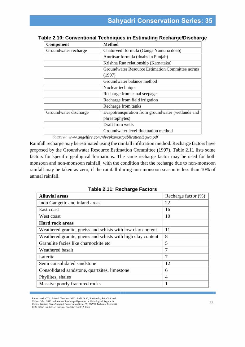
Ramachandra T.V., Subash Chandran M.D., Joshi N.V., Sreekantha, Saira V.K and
Vishnu D.M., 2013. Influence of Landscape Dynamics on Hydrological Regime in
Central Western Ghats Sahyadri Conservation Series 35, ENVIS Technical Report 65,
CES, Indian Institute of Science, Bangalore 560012, India 33
Sahyadri Conservation Series: 35
Table 2.10: Conventional Techniques in Estimating Recharge/Discharge
Component Method
Groundwater recharge Chaturvedi formula (Ganga Yamuna doab)
Amritsar formula (doabs in Punjab)
Krishna Rao relationship (Karnataka)
Groundwater Resource Estimation Committee norms
(1997)
Groundwater balance method
Nuclear technique
Recharge from canal seepage
Recharge from field irrigation
Recharge from tanks
Groundwater discharge Evapotranspiration from groundwater (wetlands and
phreatophytes)
Draft from wells
Groundwater level fluctuation method
Source: www.angelfire.com/nh/cpkumar/publication/Lgwa.pdf
Rainfall recharge may be estimated using the rainfall infiltration method. Recharge factors have
proposed by the Groundwater Resource Estimation Committee (1997). Table 2.11 lists some
factors for specific geological formations. The same recharge factor may be used for both
monsoon and non-monsoon rainfall, with the condition that the recharge due to non-monsoon
rainfall may be taken as zero, if the rainfall during non-monsoon season is less than 10% of
annual rainfall.
Table 2.11: Recharge Factors
Alluvial areas Recharge factor (%)
Indo Gangetic and inland areas 22
East coast 16
West coast 10
Hard rock areas
Weathered granite, gneiss and schists with low clay content 11
Weathered granite, gneiss and schists with high clay content 8
Granulite facies like charnockite etc 5
Weathered basalt 7
Laterite 7
Semi consolidated sandstone 12
Consolidated sandstone, quartzites, limestone 6
Phyllites, shales 4
Massive poorly fractured rocks 1

Ramachandra T.V., Subash Chandran M.D., Joshi N.V., Sreekantha, Saira V.K and
Vishnu D.M., 2013. Influence of Landscape Dynamics on Hydrological Regime in
Central Western Ghats Sahyadri Conservation Series 35, ENVIS Technical Report 65,
CES, Indian Institute of Science, Bangalore 560012, India 34
Sahyadri Conservation Series: 35
In this method, all components of the groundwater balance equation, except the rainfall
recharge, are estimated individually. This method requires extensive and accurate hydrological
and meteorological data. This method is valid for areas where the year can be divided into
monsoon and non-monsoon months with the bulk of the rainfall occurring during the monsoon
months.
Soil moisture data based method consists of soil water balance method and nuclear methods.
Soil water balance method consists of lumped and distributed models. In the lumped model,
the variation of soil moisture content in the vertical direction is ignored and any effective input
into the soil is assumed to increase the soil moisture content uniformly. In the distributed
model, variation of soil moisture content in the vertical direction is accounted and the method
involves the numerical solution of partial differential equation (Richards equation) governing
one-dimensional flow through unsaturated medium, with appropriate initial and boundary
conditions.
Water balance models were developed by Thornthwaite (1948) and later revised by
Thornthwaite and Mather. The method is essentially a bookkeeping procedure, which estimates
the balance between the inflow and outflow of water. The disadvantage of this method is that
when applying this method to estimate the recharge for a catchment area, the calculation should
be repeated for areas with different precipitation, evapotranspiration, crop type and soil type.
Results from this model are of very limited value without calibration and validation, because
of the substantial uncertainty in the input data.
Nuclear techniques can also be used for the determination of recharge by measuring the travel
time of moisture through a soil column (www.angelfire.com/nh/cpkumar/
publication/Lgwa.pdf). A mixture of Beryllium (Be) and Radium (Ra) is taken as the source of
neutrons. Another method is the gamma ray transmission method based upon the attenuation
of gamma rays in a medium through which it passes. The extent of attenuation is closely linked
with moisture content of the soil medium.
Water requirements of crops are met by rainfall, soil moisture and irrigation water. Recharge
from irrigation fields are estimated from water balance method. For a correct assessment of the
quantum of recharge by applied irrigation, studies are required to be carried out on
experimental plots under different crops in different seasonal conditions. Groundwater
Resource Estimation Committee has proposed the following standards in percentages for crop
such as paddy watered either by surface water and groundwater given in Table 2.12.

Ramachandra T.V., Subash Chandran M.D., Joshi N.V., Sreekantha, Saira V.K and
Vishnu D.M., 2013. Influence of Landscape Dynamics on Hydrological Regime in
Central Western Ghats Sahyadri Conservation Series 35, ENVIS Technical Report 65,
CES, Indian Institute of Science, Bangalore 560012, India 35
Sahyadri Conservation Series: 35
Table 2.12: Recharge Factors for Crops
Source of
irrigation
Type of crop Water table below ground surface
< 10m 10-25m > 25m
Groundwater Non paddy 25 (%) 15 (%) 5 (%)
Surface water Non paddy 30(%) 20 (%) 10 (%)
Groundwater Paddy 45 (%) 35 (%) 20 (%)
Surface water Paddy 50 (%) 40 (%) 25 (%)
Groundwater can be discharged by evapotranspiration from wetlands and phreatophytic
vegetation. The potential evapotranspiration from such areas can be computed using standard
methods and the discharge estimated.
Groundwater is essentially a subsurface phenomenon and the common current remote sensing
platforms record features on the surface (Meijerink, 2000). Most of the information for
groundwater, as yet has to be obtained by qualitative reasoning and semi-quantitative
approaches.
Image interpretations are used to locate areas where the groundwater table is probably shallow.
The appearance of groundwater at or near the surface is caused by either the intersection of
topographic depressions or a static phreatic groundwater level or by discharge zone of an
upwelling groundwater flow system. In both cases, there will be an effect on vegetation,
relative soil moisture, land use or on details of the drainage systems and these effects can be
identified on remotely sensed imageries.
With this in mind, groundwater discharge can be estimated by determining evapotranspiration
from phreatophytes and wetlands (D’Agnese et al, 1996) Phreatophytes are plants whose roots
can tap water from the groundwater table and thus are indicators of the presence of shallow
groundwater.
Various indices have been used to map various types of vegetation such as phreatophytes,
wetland vegetation and riparian vegetation which discharge groundwater through
evapotranspiration. Among these are perpendicular vegetation index (PVI), greenness
vegetation index (GVI), transformed vegetation index (TVI) etc. PVI is used (mainly used in
arid regions) to minimize the effects of soil reflectance in low-density vegetation communities.
GVI is used to distinguish between different levels of greenness while minimizing effects of
soil brightness and TVI is used to produce vegetation density map and to discriminate between
light coloured soils and dead or dying vegetation.

Ramachandra T.V., Subash Chandran M.D., Joshi N.V., Sreekantha, Saira V.K and
Vishnu D.M., 2013. Influence of Landscape Dynamics on Hydrological Regime in
Central Western Ghats Sahyadri Conservation Series 35, ENVIS Technical Report 65,
CES, Indian Institute of Science, Bangalore 560012, India 36
Sahyadri Conservation Series: 35
Recharge in dry areas can be promoted by the presence of mountains. Typically, precipitation
is greater at higher elevations (concept of Maxey-Eakin method) and relief promotes rapid and
efficient runoff. Water running off the mountains effectively infiltrates alluvial fans bordering
the mountain ranges. Alluvial fan sediments are highly permeable. A modified Maxey-Eakin’s
method has been derived that calculates a recharge potential map from slope, elevation, soil
permeability and vegetation map. It is expressed as a percentage and is further multiplied with
average annual precipitation (D’Agnese et al, 1996).
Land use and its Effect on Hydrology: Human activities have been recognized as a major
force shaping the biosphere in recent years. Human actions rather than natural forces are the
source of most contemporary change in the states and flows of the biosphere (Turner and Meyer
1994). Understanding these actions and the social forces that drive them is thus of crucial
importance for understanding, modeling and predicting environmental change and for
managing and responding to such change.
Concerns about land use/land cover change emerged in the research agenda on global
environmental change several decades ago with the realization that land surface processes
influence climate (Lambin et al., 2003). In the mid 1970s, it was recognized that land cover
change modifies surface albedo and thus surface-atmosphere energy exchanges, which have an
impact on regional climate. In the 1980s, terrestrial ecosystems as carbon sources and sinks
were highlighted and later the important contribution of local evapotranspiration to the water
cycle-that is precipitation recycling-as a function of land use/land cover highlighted yet another
considerable impact of land use/land cover change on the climate. A much broader range of
impacts of land use/land cover change on ecosystem goods and services were further identified
(Lambin, et al., 2003). Of primary concern are impacts on biotic diversity worldwide, soil
degradation and the ability of biological systems to support human needs. It also determines
the vulnerability of places and people to climatic, economic or sociopolitical disturbances.
Thus, it becomes necessary to estimate the temporal and spatial development of land use
changes to assess their impact on the ecosystems and the environment. A most efficient way of
capturing the spatial and temporal details is by remote sensing. Hydrological models coupled
with remote sensing data can efficiently characterize temporal and spatial effects of land use
changes on the ecology and hydrology.
Changes in land cover alters the hydrological cycle and in most of the mass and energy fluxes
that sustain the biosphere and geosphere. Due to agriculture, forest management and
urbanisation, the physical characteristics of the land surface and upper soil as well as the
transpiration process that is strongly related to the type of vegetation are changed. As a result
the amount of runoff, the soil moisture and groundwater recharge are also strongly affected.

Ramachandra T.V., Subash Chandran M.D., Joshi N.V., Sreekantha, Saira V.K and
Vishnu D.M., 2013. Influence of Landscape Dynamics on Hydrological Regime in
Central Western Ghats Sahyadri Conservation Series 35, ENVIS Technical Report 65,
CES, Indian Institute of Science, Bangalore 560012, India 37
Sahyadri Conservation Series: 35
Some of the effects of land use changes such as changes in forest cover, agricultural activities
and urbanisation are discussed below:
Felling trees for the combined objectives of obtaining wood for construction, shelter and tool
making; of providing fuel to keep warm, to cook food, and to smelt metals; and above all, of
creating land for growing food, has culminated in one of the main processes whereby
humankind has modified the world’s surface cover of vegetation (Williams, 1994). Forests
covered about half of the earth’s surface up to the development of early civilizations but today
cover less than one-third of that area (FAO, 1993). Between 1980 and 1995, the extent of the
world’s forests decreased by some 180 million ha, an area about the size of Indonesia or
Mexico. This represents a global annual loss of 12 million ha, an area equivalent to the size of
Greece or Bangladesh (Ball, 2001). During this 15-year period, developing countries lost nearly
200 million ha of natural forests, mostly through clearing for agriculture (shifting cultivation,
other forms of subsistence agriculture, and the establishment of cash crop plantations such as
oil palm and ranching).
Forest cover influences climatic and soil conditions and therefore the amount of water flowing
from forested areas (Bruijnzeel, 2001). As compared with grass or low vegetation, forests may
exert a major influence on what happens to the precipitation once it reaches the ground. Rain
may be redistributed to some degree, although this effect is probably more important for local
vegetation patterns than it is for any influence on water yield and timing. When there is rainfall
of sufficient intensities, a large portion of total storm precipitation will eventually reach the
ground, although it may be redistributed by stem-flow and drippage. That portion of the rainfall
intercepted by the vegetation canopies eventually evaporates, reducing transpiration.
The following sections will discuss some aspects of the hydrological effects of i) forest clear
felling on water yield and stream flow regimes and ii) effects of reforestation.
i) Effects of forest clear felling on water yield and stream flow regimes: Total annual water
yield appears to increase with the percentage of forest biomass removed, but actual amounts
differ between sites and years due to difference in rainfall and the degree of surface disturbance
(Bruijnzeel, 2004). If surface disturbance remains limited most of the water yield increase
occurs as lowflows (baseflows), but in the long term, rainfall infiltration is reduced to the extent
that insufficient rainy season replenishment of groundwater reservoirs results in strong declines
in the dry season flows. Reports of greatly diminished stream flow during the dry season after
forest clear felling abound in the literature, particularly in the tropics. The continued exposure
of bare soil after forest clearing to intense rainfall, the compaction of topsoil by machinery, or
overgrazing, the gradual disappearance of soil faunal activity and increases in the area occupied

Ramachandra T.V., Subash Chandran M.D., Joshi N.V., Sreekantha, Saira V.K and
Vishnu D.M., 2013. Influence of Landscape Dynamics on Hydrological Regime in
Central Western Ghats Sahyadri Conservation Series 35, ENVIS Technical Report 65,
CES, Indian Institute of Science, Bangalore 560012, India 38
Sahyadri Conservation Series: 35
by impervious surfaces such as roads and settlements, all contribute to gradually reduced
rainfall infiltration opportunities in cleared areas. As a result, catchment response to rainfall
becomes more pronounced and the increases in storm runoff during the rainy season may
become large as to seriously impair the recharging of soil water and ground water. When this
critical stage is reached, the result is diminished dry season flow. It should be noted that
comparing stream flow totals for catchments with contrasting land use types might produce
misleading results because of the possibility of geologically determined differences in
catchment groundwater reserves or deep leakage. Catchments underlain by sandstones,
limestones, basalts and volcanic tuffs are noted for this. Under mature tropical rain forest,
typically 80-95% of incident rainfall infiltrates into the soil, of which around 1000 mm per year
is transpired again by the trees when soil moisture is not limiting, whereas the remainder is
used to sustain stream flow. As such the bulk of the increase in flow upon clearing in the form
of baseflow, as long as the intake capacity of the surface soil is not impaired too much
(Bruijnzeel, 1990).
ii) Effect of reforestation: Water yields have been reported to return to original levels within 8
years where pine plantations replaced natural forest such as in upland Kenya (Blackie,
1979a,b). Bruijnzeel, 1997 have pointed out the lack of sufficient information about the
hydrological consequences of planting fast growing tree plantation species such as Acacia
mangium, Gmelina arborea, Paraserianthes falcatarai and Eucalyptus spp. and pines. Recent
observations in 10 year old stands have confirmed the high water use of Acacia mangium in
East Malaysia even during a period of drought (Cienciala et al., 2000). Plantations of
Eucalyptus camaldulensis and Eucalyptus tereticornis in southern India exhibited similar
behaviour with transpiration rates upto 6 mm per day when unrestricted by soil water deficits
at the end of the monsoon, although values fell to 1 mm per day when soil water contents were
low during the subsequent long dry seasons (Roberts and Rosier, 1993).
Historically, humans have increased agricultural output mainly by bringing more land into
production. The mix of cropland expansion and agricultural intensification has varied
geographically (UN FAO, 2001). Despite claims to the contrary, the amount of suitable land
remaining for crops is very limited in most developing countries (Young, 1999). The main
hydrological effect of cropped land is a change in the partitioning of the rainfall into
evaporation, overland flow, and infiltration. In places where irrigation is practiced, typically
80-90% of the water is ‘consumed’ or evapotranspired (not returned to flow) by irrigation.
Irrigation therefore has a greater impact on the hydrological cycle. Activities such as land
improvement, land drainage, merging of small areas, as well as the type of tillage, type of crop
cultivated, simplification of crop rotation, single-crop farming, etc. can disturb the water
balance of rural areas (decrease in the groundwater renewal rate, decrease in the groundwater
table, increase of water discharge, etc.) and increases the risk of erosion (erosion caused by

Ramachandra T.V., Subash Chandran M.D., Joshi N.V., Sreekantha, Saira V.K and
Vishnu D.M., 2013. Influence of Landscape Dynamics on Hydrological Regime in
Central Western Ghats Sahyadri Conservation Series 35, ENVIS Technical Report 65,
CES, Indian Institute of Science, Bangalore 560012, India 39
Sahyadri Conservation Series: 35
precipitation, wind-erosion, mudflow, flooding (inundation). Soil compaction due to
movement of heavy vehicles and deterioration of the soil structure increases the surface runoff
and, therefore, will reduce the groundwater renewal rate of the area. The increase of biomass
of the crops increases the water consumption and therefore reduces the soil moisture and the
groundwater renewal rate. In some regions often the associated irrigation completes the
increased water demand. The main causes of increased erosion are seen as single-crop farming,
simplification of crop rotation, soil compaction, changing from grassland to arable land and
land drainage. This will reduce the water storage capacity and the filtration capability of the
soil, and the surrounding surface waters may become eutrophic.
Settlement represents the most profound alteration of the natural environment by people
through the imposition of structures, buildings, paved surfaces and compacted bare soils on the
ground surface (Douglas, 1994). Settlements also lead to other land cover changes, such as the
storage of water in reservoirs; the removal of vegetation and soil to extract sand, gravel, brick
clays and rock; and the use of land for transportation routes. Urban and suburban development
of forested watersheds can increase the percentage of impervious surfaces on a watershed from
nearly zero in a rural setting to, almost 100 percent in commercial or industrial areas. It can be
concluded that urbanization in forested watersheds tend to reduce interception, infiltration, soil-
moisture storage and evapotranspiration, and increases overland flow. Several studies of peak
flows have shown that they may be increased by 1.2 to 5 times over peaks from rural conditions.
During development and construction of suburban areas, sedimentation may be increased
greatly; even after construction, sedimentation in these areas may be 5 to 10 times that from
protected watersheds. They also find that annual maximum peak flows increase, although
maximum daily flows decrease. Total flow volume increases because a greater percentage of
summer precipitation appears as runoff, while protected stream banks will yield minimum
impacts (http://samab.org/saa/reports/aquatic/chapter5.pdf).
Even through tropical rural people are much more vulnerable to perturbations of the natural
environment than their urban counterparts, they have large collective impacts on the natural
world. In great areas of paddy cultivation and irrigation agriculture of Asia, the whole
landscape is a pattern of fields, water channels and settlements. Water flows are usually tightly
controlled. Settlements in these areas are often compact to maximize the amount of land
available for cultivation. In areas cultivated or grazed less intensively, rural settlements may
sprawl and have crop production intermingled with the houses. A tightly knit series of
dwellings with only compacted ground between them will modify the radiation balance and the
hydrological cycle much more than a dispersed village with gardens all around the house and
trees shading much of the roof area.

Ramachandra T.V., Subash Chandran M.D., Joshi N.V., Sreekantha, Saira V.K and
Vishnu D.M., 2013. Influence of Landscape Dynamics on Hydrological Regime in
Central Western Ghats Sahyadri Conservation Series 35, ENVIS Technical Report 65,
CES, Indian Institute of Science, Bangalore 560012, India 40
Sahyadri Conservation Series: 35
Another major land use change is the construction of dams and reservoirs for hydro electrical
power, flood control, irrigation and water supply. In the past half-century, dams and reservoirs
have become an increasingly important part of anthropogenic land cover change. Today there
are over 45,000 large dams (dams over 15 m height, or with reservoirs containing 3 million
cubic meters of water), and total annual freshwater withdrawals today are estimated at 3,800
cubic km, twice as much as 50 years ago. Even though they make up only a small percentage
of total land cover, these artificial water bodies often facilitate other forms of land cover
change, such as development of large-scale irrigated areas and urbanization that cover far larger
areas. According to the World Commission on Dams (2000), large dams can have numerous
impacts on ecosystems. These include the loss of forests and wildlife habitat, the loss of species
populations and the degradation of upstream catchment areas due to inundation of the reservoir
area; the loss of aquatic biodiversity, of upstream and downstream fisheries, and of the services
of downstream floodplains, wetlands, and riverine, estuarine and adjacent marine ecosystems;
and cumulative impacts on water quality, natural flooding and species composition where a
number of dams are sited on the same river.
Furthermore, dams and reservoirs impact the hydrological cycle by increasing evaporation
(dams in arid areas can lose 5 percent of total withdrawals to evaporation) and loss of
downstream aquifers due to reduced replenishment. Environmental flow requirements (which
include managed flood releases) are increasingly used to reduce the impacts of changed stream
flow regimes on aquatic, floodplain and coastal ecosystems, downstream. Sedimentation and
the consequent long-term loss of water storage is a serious concern globally, and the effects
will be particularly felt by basins with high geological or human-induced erosion rates. Thus,
land cover change that promotes increasing sediment loads, such as agricultural land uses or
deforestation, affect the water storage and electricity generation capacity of dams.

Ramachandra T.V., Subash Chandran M.D., Joshi N.V., Sreekantha, Saira V.K and
Vishnu D.M., 2013. Influence of Landscape Dynamics on Hydrological Regime in
Central Western Ghats Sahyadri Conservation Series 35, ENVIS Technical Report 65,
CES, Indian Institute of Science, Bangalore 560012, India 41
Sahyadri Conservation Series: 35
3.0 Study Area
Sharavathi river rises at Ambuteertha, near Kavaledurga in Tirthahalli taluk. It flows in a
northwesterly direction and receives the Haridravathi on the right and Yenneholé on the left.
Near the border the district, it bends to the west and hurls down the ghats near Jog where it is
harnessed for generating electricity. It discharges into the sea at Honnavar in Uttara Kannada.
It’s total length is 128 km and in Shimoga district its length is 32.2 km. According to a legend,
the name Sharavathi means ‘arrow-born’ and the river was formed from a dart of
Ramachandra’s arrow (KSG, 1975). Figure 3.1 depicts the location of the study area in India
and Karnataka.
Figure 3.1: Study Area – Sharavathi river basin
Uttara
Kannada
Shimoga
India with location
of Karnataka
Uttara Kannada and Shimoga districts
with Sharavathi River Basin Boundary
Karnataka with location of
Uttara Kannada and Shimoga
Arabian
Sea
Uttara
Kannada
Shimoga

Ramachandra T.V., Subash Chandran M.D., Joshi N.V., Sreekantha, Saira V.K and
Vishnu D.M., 2013. Influence of Landscape Dynamics on Hydrological Regime in
Central Western Ghats Sahyadri Conservation Series 35, ENVIS Technical Report 65,
CES, Indian Institute of Science, Bangalore 560012, India 42
Sahyadri Conservation Series: 35
Figure 3.2: Sharavathi River Basin –Upstream and Downstream
Figure 3.3: Upstream River Basin
Upstream
Downstream
Linganamakki
Reservoir
Sharavathi
River

Ramachandra T.V., Subash Chandran M.D., Joshi N.V., Sreekantha, Saira V.K and
Vishnu D.M., 2013. Influence of Landscape Dynamics on Hydrological Regime in
Central Western Ghats Sahyadri Conservation Series 35, ENVIS Technical Report 65,
CES, Indian Institute of Science, Bangalore 560012, India 43
Sahyadri Conservation Series: 35
3.1 Topography
Sharavathi river basin falls in two districts namely Uttara Kannada and Shimoga. Upstream
river basin extends to two taluks in Shimoga viz. Hosanagara and Sagara. The entire basin has
an area of 2985.66 km2 with upstream and downstream respectively are 1988.99 km2 and
996.67 km2 each. The basin slopes from west to east. The general elevation along the basin is
about 640 m above sea level in the west
The western side of the upstream river basin rests upon the Western Ghats also known as the
Sahyadri, which is a very mountainous area. The raise towards the crest of the Ghats is very
rapid, a height of 1343 meters according to the Survey of India, being attained at Kodachadri.
The southwestern portion of Sagar taluk presents the appearance of a rolling stretch of bare hill
tops, the sides and valleys of which are densely wooded. The Hosanagara taluk is enclosed on
three sides by hills, the drainage of which flows northwest into the Sharavathi (KSG, 1975).
Figure 3.4 gives the digital elevation model of upstream.
Figure 3.4: Digital Elevation Model
Slope percentage map derived from digital elevation model was classified into various slope
groups.

Ramachandra T.V., Subash Chandran M.D., Joshi N.V., Sreekantha, Saira V.K and
Vishnu D.M., 2013. Influence of Landscape Dynamics on Hydrological Regime in
Central Western Ghats Sahyadri Conservation Series 35, ENVIS Technical Report 65,
CES, Indian Institute of Science, Bangalore 560012, India 44
Sahyadri Conservation Series: 35
Table 3.1: Slope Classifications
Slope in percentage Slope group
0-10 Nearly flat
10-15 Gently sloping
15-20 Moderately sloping
20-30 Strongly sloping
30-80 Steep sloping
Figure 3.5 classifies slope map into 5 major slope groups. This classification is given in Table
3.1. Steep to strongly sloping are characteristics of malnadu (mountainous region) on the
western side and is covered by dense vegetation such as evergreen/semievergreen and moist
deciduous forests. Slopes attain nearly level ground at the centre of the basin (reservoir) and
gently slopes upward towards the east. Eastern portion especially Haridravathi and Nandiholé
sub basins consists of nearly level or flat land, where paddy cultivation is practiced.
Figure 3.5: Slope Classification

Ramachandra T.V., Subash Chandran M.D., Joshi N.V., Sreekantha, Saira V.K and
Vishnu D.M., 2013. Influence of Landscape Dynamics on Hydrological Regime in
Central Western Ghats Sahyadri Conservation Series 35, ENVIS Technical Report 65,
CES, Indian Institute of Science, Bangalore 560012, India 45
Sahyadri Conservation Series: 35
3.2 Geology
The geology of Sharavathi river basin consists of Pre-Cambrian rocks, which are devoid of
fossils. Apart from being heterogeneous in their origin (consolidated intrusive magmas, ancient
sediments, volcanic rocks) they were more less thoroughly reshuffled by new intrusions, faults
and metamorphism (Pascal, 1988). The two major groups of rocks found in the study area are
the Dharwar system and the peninsular gneiss.
The Dharwar system: It is named after the township of Dharwar on the Karnataka plateau. This
system includes metamorphic rocks that are considered to be among the oldest in India. These
rocks are derived from metamorphosed ancient sediments: conglomerates, more or less
ferruginous quartzites, greywackes, schists and limestones. They are rich in iron and
manganese and sometimes in copper, lead and gold too.
Peninsular gneiss: These are crystalline rocks and consist of a heterogeneous mixture of gneiss
and different kinds of intrusive granites. They are made up of granite, granodiorite, granito-
gneiss, migmtatite etc. These ‘peninsular gneiss’ are encountered almost all along the Ghats
but they are predominant only between 110N and 140N.
Geology map of Sharavathi upstream river basin given in Figure 3.6, has been created by
combining the geology map of Department of Mines and Geology and the French Institute.
This has been done for simplification of groundwater analysis
Figure 3.6: Geology

Ramachandra T.V., Subash Chandran M.D., Joshi N.V., Sreekantha, Saira V.K and
Vishnu D.M., 2013. Influence of Landscape Dynamics on Hydrological Regime in
Central Western Ghats Sahyadri Conservation Series 35, ENVIS Technical Report 65,
CES, Indian Institute of Science, Bangalore 560012, India 46
Sahyadri Conservation Series: 35
3.3 Drainage and Sub basins
As can be seen from Figure 3.7, dense drainage network is observed in the western portion of
the basin. These are areas of very steep to steep slopes. Eastern portion especially, Nandiholé
and Haridravathi basins are characterized by less dense network due to the gentle slope. The
pattern of drainage in the basin is mainly dendritic. Dendritic drainage pattern takes the form
of "dendrites" and looks like the branching roots of a tree. In areas of high permeability soil
such as sand viz. in Haridravathi and Nandiholé, the drainage density is low as compared with
low permeability soil (clay) and high drainage density on the western side e.g. Yenneholé,
Hurliholé etc. Drainage density is the ratio between the total length of the stream and the area
drained by them.
Figure 3.7: Drainage
Sub-basins have been delineated according to the main tributaries flowing into the reservoir
as depicted in Figure 3.8.
3.4 Climate
The climate in the study area is characterized by the monsoon regime, which superimposes
itself over a regime of thermic convectional rainfall lined to the zenithal passage of the sun.
The cold season is from December to February and is followed by the hot season which is from
March to May.

Ramachandra T.V., Subash Chandran M.D., Joshi N.V., Sreekantha, Saira V.K and
Vishnu D.M., 2013. Influence of Landscape Dynamics on Hydrological Regime in
Central Western Ghats Sahyadri Conservation Series 35, ENVIS Technical Report 65,
CES, Indian Institute of Science, Bangalore 560012, India 47
Sahyadri Conservation Series: 35
a) Rainfall: The rainfall is very heavy in the region of Western Ghats especially along the
western side of the river basin. Mean annual rainfall ranges from 6000mm in the
western side to 1700mm in the eastern side of the basin. About 95% of the rainfall is
received during the south west monsoon months, June to September, July being rainiest
(KSG, 1975). There is some rainfall in the post monsoon season, particularly in
October, and it is mostly in the form of thundershowers. Some rainfall in the form of
thundershowers also occurs during the summer months of April and May.
b) Temperature: After January, there is a rapid increase of temperatures. April is usually
the hottest month with the mean daily maximum temperature at 35.8oC and the mean
daily minimum at 22.2oC.
c) Humidity: The relative humidity during the mornings throughout the year generally
exceeds 75%. During the monsoon months, the relative humidity in the afternoon is
quite high and is ~60 %. The driest part of the year is the period from January to March
when the relative humidity in the afternoon is less than 35%.
d) Winds: It is generally light with some increase in force during the monsoon season.
Winds are mostly from directions between northwest and southwest during the period
May to September. In the rest of the year, they are predominantly from the south east.
Figure 3.8: Sub basins of Upstream
Linganamakki
Nandiholé
Haridravathi Mavinaholé
Sharavathi
Hilkunji
Hurliholé
Nagodiholé
Yenneholé

Ramachandra T.V., Subash Chandran M.D., Joshi N.V., Sreekantha, Saira V.K and
Vishnu D.M., 2013. Influence of Landscape Dynamics on Hydrological Regime in
Central Western Ghats Sahyadri Conservation Series 35, ENVIS Technical Report 65,
CES, Indian Institute of Science, Bangalore 560012, India 48
Sahyadri Conservation Series: 35
3.5 Soil
i) Four soil orders are found in upstream viz. ultisols, alfisols, inceptisols and entisols.
ii) Moisture regime of the soils in upstream river basin is characterized by an ustic
moisture regime.
Ustic moisture regime: (ustic-burnt)-Ustic moisture regime is one that is limited but is
present at a time when conditions are suitable for plant growth. It means that the soil is dry in
some or all parts for 90 days or more in normal years and moist in some parts either for 90 days
or more consecutive days or 180 cumulative days per year. Moisture regime is ustic in tropical
and subtropical regions if there is atleast one rainy season of 3 months or more.
ii) Soils in upstream are classified as isohyperthermic (mean annual temp 220C).
iii) The soils of Western Ghats are generally dark to brown to dark reddish brown and
black in colour due to accumulation of high organic matter under forests cover.
Table 3.2 gives the soil taxonomy of upstream river basin.
Table 3.2 Soil Taxonomy of Sharavathi Upstream River Basin
Order Sub order Great groups Sub groups
Alfisols Ustalfs Kandiustalfs
Haplustalfs
Paleustalfs
Typic kandiustalfs
Kanhaplic haplustalfs
Kandic paleustalfs
Ultisols Humults Palehumults
Kandihumults
Ustic palehumults
Ustic kandihumults
Inceptisols Tropepts Dystropepts
Ustropepts
Ustoxic dystropepts
Aquic ustropepts
Entisols Fluvents Ustifluvents Aquic ustifluvents

Ramachandra T.V., Subash Chandran M.D., Joshi N.V., Sreekantha, Saira V.K and
Vishnu D.M., 2013. Influence of Landscape Dynamics on Hydrological Regime in
Central Western Ghats Sahyadri Conservation Series 35, ENVIS Technical Report 65,
CES, Indian Institute of Science, Bangalore 560012, India 49
Sahyadri Conservation Series: 35
Figure 3.9: Soil Texture
3.6 Groundwater Conditions
Groundwater is present in the voids of rocks and soil and is an important source of irrigation
in the basin. Figure 3.10 maps the wells in the region.
Figure 3.10: Location of Selected Wells in Upstream

Ramachandra T.V., Subash Chandran M.D., Joshi N.V., Sreekantha, Saira V.K and
Vishnu D.M., 2013. Influence of Landscape Dynamics on Hydrological Regime in
Central Western Ghats Sahyadri Conservation Series 35, ENVIS Technical Report 65,
CES, Indian Institute of Science, Bangalore 560012, India 50
Sahyadri Conservation Series: 35
3.7 Vegetation and Agricultural Activities
Evergreen-semievergreen forests are confined to the western part of the basin. Many of the
hills are covered with heavy forests while ravines and valleys produce luxuriant trees known
for their great height and size (KSG, 1975). Scattered shrubs and thickets are found in the
regions surrounding the reservoir. Moist deciduous forests are found in the northern and
eastern part of the study area.
Plantations include acacia, teak, areca, rubber, eucalyptus etc. Areca nut also called betel nut
is a widely used article of consumption and is grown in valleys. Acacia plantation is found in
patches, amidst evergreen forests and is mainly used for paper production. Plantation
constitutes 7-9% of the total vegetation in the upstream. Evergreen /semievergreen and moist
deciduous forests constitutes 11% and 25% respectively.
Paddy and areca are cultivated extensively in eastern parts of the upstream. Paddy is grown as
a kharif crop and some pulses are grown during the rabi season. Rabi season is short and the
land is mostly left fallow. Paddy is grown under rainfed and irrigated conditions both in kharif
and summer season. In irrigated areas, paddy cultivation is followed by sugarcane during kharif
season.

Ramachandra T.V., Subash Chandran M.D., Joshi N.V., Sreekantha, Saira V.K and
Vishnu D.M., 2013. Influence of Landscape Dynamics on Hydrological Regime in
Central Western Ghats Sahyadri Conservation Series 35, ENVIS Technical Report 65,
CES, Indian Institute of Science, Bangalore 560012, India 51
Sahyadri Conservation Series: 35
Figure 3.11: Upstream River Basin
Sharavathi River Part of Linganamakki reservoir
Island inside the reservoir (rainy
season)
Island inside the reservoir (summer
season)
Ambuthirtha- Origin of Sharavathi River Thick evergreen forests at Nagodiholé

Ramachandra T.V., Subash Chandran M.D., Joshi N.V., Sreekantha, Saira V.K and
Vishnu D.M., 2013. Influence of Landscape Dynamics on Hydrological Regime in
Central Western Ghats Sahyadri Conservation Series 35, ENVIS Technical Report 65,
CES, Indian Institute of Science, Bangalore 560012, India 52
Sahyadri Conservation Series: 35
Portions of former submerged
forest seen during the dry season Another view
Teak plantations Portions of cleared forest
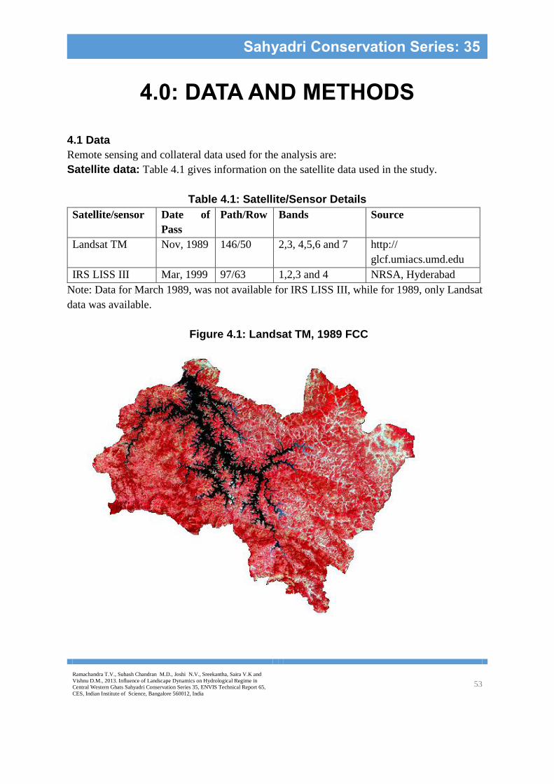
Ramachandra T.V., Subash Chandran M.D., Joshi N.V., Sreekantha, Saira V.K and
Vishnu D.M., 2013. Influence of Landscape Dynamics on Hydrological Regime in
Central Western Ghats Sahyadri Conservation Series 35, ENVIS Technical Report 65,
CES, Indian Institute of Science, Bangalore 560012, India 53
Sahyadri Conservation Series: 35
4.0: DATA AND METHODS
4.1 Data
Remote sensing and collateral data used for the analysis are:
Satellite data: Table 4.1 gives information on the satellite data used in the study.
Table 4.1: Satellite/Sensor Details
Satellite/sensor Date of
Pass
Path/Row Bands Source
Landsat TM Nov, 1989 146/50 2,3, 4,5,6 and 7 http://
glcf.umiacs.umd.edu
IRS LISS III Mar, 1999 97/63 1,2,3 and 4 NRSA, Hyderabad
Note: Data for March 1989, was not available for IRS LISS III, while for 1989, only Landsat
data was available.
Figure 4.1: Landsat TM, 1989 FCC

Ramachandra T.V., Subash Chandran M.D., Joshi N.V., Sreekantha, Saira V.K and
Vishnu D.M., 2013. Influence of Landscape Dynamics on Hydrological Regime in
Central Western Ghats Sahyadri Conservation Series 35, ENVIS Technical Report 65,
CES, Indian Institute of Science, Bangalore 560012, India 54
Sahyadri Conservation Series: 35
Figure 4.2: IRS LISS III, 1999 FCC
Note: TM – Thematic Mapper
IRS - Indian Remote Sensing Satellite
LISS - Linear Imaging Self Scanning
Toposheets: Survey of India toposheets of scale 1:50,000 have been used for geo referencing
remote sensing data as well as for field investigations. Table 4.2 gives the list of toposheets
used for the study.
Table 4.2: Toposheets of Upstream River Basin
48 J/14
48 J/11 48 J/15
48 J/12 48 J/16 48 N/4 48 N/8
48 K/9 48 O/1 48 O/5
48 O/2 48 O/6
48 O/3
Field and Ancillary Data: GPS points along with attribute information were collected
upstream to determine the type of land cover and land use such as vegetation, which includes

Ramachandra T.V., Subash Chandran M.D., Joshi N.V., Sreekantha, Saira V.K and
Vishnu D.M., 2013. Influence of Landscape Dynamics on Hydrological Regime in
Central Western Ghats Sahyadri Conservation Series 35, ENVIS Technical Report 65,
CES, Indian Institute of Science, Bangalore 560012, India 55
Sahyadri Conservation Series: 35
evergreen-semievergreen and moist deciduous forests and plantations, degraded vegetation,
agricultural activities, settlements, etc.
Maps and other ancillary used for the study include:
i) Forest Map of South India (1982) by J.P. Pascal, French Institute of Pondicherry.
ii). Soil map published by the National Bureau of Soil Survey.
iii). Reconnaissance Soil Map of Forest Area, Western Karnataka and Goa
iv) Geology map, Department of Mines and Geology
v) Bioclimate of the Western Ghats (1982), J.P.Pascal, French Institute of Pondicherry.
Climate data:
i) IMD Talukwise rainfall data (1901-2001) for Sagara, Hosanagara, Soraba and
ii) Tirthahalli (Shimoga) and Honnavara, Kumta and Siddapur (Uttara Kannada).
iii) Daily rainfall data from Karnataka Power Corporation Limited for 18 rain gauge
stations in Sharavathi river basin (1989-1999).
iv) IMD maximum and minimum temperature data (1969-2000) for Shimoga.
v) IMD extraterrestrial solar radiation and number of sunshine hours for Shimoga
vi) (1989-1999).
vii) Water table level data (1989-1999) for selected wells in and around the study area
viii) from Dept. of Mines and Geology.
4.2 Remote sensing data Analysis
4.2.1 Image Rectification and Restoration - This involves the initial processing of raw
image data to correct for geometric distortions, to calibrate the data radiometrically and to
eliminate the noise present in the data. In this study random and residual unknown systematic
distortion are corrected by analysing well-distributed ground control points collected from
known ground locations and GPS points in terms of latitude and longitude. These values are
then submitted to a least squares regression analysis to determine coefficients for two co-
ordinate transformation equations that can be used to interrelate the geometrically correct
(map) coordinated and the distorted image co-ordinates (Lillesand and Kiefer, 2002).
Expressing this in mathematical notation,
x = f1(X,Y) y = f2 (X,Y) (4.1)
(x,y) – distorted image co-ordinates (column, row)
(X,Y) –corrected (map) co-ordinates
f1,f2 – transformation functions
The next step is to decide how best to estimate the values of pixels in the corrected image based
upon information in the uncorrected image. This is done through resampling, using nearest

Ramachandra T.V., Subash Chandran M.D., Joshi N.V., Sreekantha, Saira V.K and
Vishnu D.M., 2013. Influence of Landscape Dynamics on Hydrological Regime in
Central Western Ghats Sahyadri Conservation Series 35, ENVIS Technical Report 65,
CES, Indian Institute of Science, Bangalore 560012, India 56
Sahyadri Conservation Series: 35
neighbour technique as it was considered computationally most efficient and also due to its
simplicity and ability to preserve original values in the unaltered scene.
Creation of false colour composite consisted of assigning colours to gray values from near
infrared, red and green bands. This helped in identifying heterogeneous patches, which were
chosen for ground data collection (training polygons).
4.2.2 Image Classification
The objective of this operation is to replace visual analysis of the image data with quantitative
techniques for automating the identification of features in a scene. This normally involves the
analysis of multispectral image data and application of statistically based decision. Common
classification procedures can be broken down into two broad subdivisions: supervised
classification and unsupervised classification.
In unsupervised classification, spectral classes are grouped first, based solely on numerical
information in the data, and are then matched by the analyst to information classes (if possible).
The basic premise is that values within a given cover type should be close together in the
measurement space whereas data in different classes should be comparatively well separated.
Unsupervised classification involves clustering algorithms that examine the unknown pixels in
an image and aggregate them into a number of classes based on the natural groupings or clusters
present in the image values (Lillesand and Kiefer, 2002).
In a supervised classification, homogeneous representative samples of the different surface
cover types (information classes) of interest are identified. These samples are referred to as
training areas. The selection of appropriate training areas is based on the knowledge of the
geographical area and actual surface cover types present in the image. The computer uses a
special program or algorithm (of which there are several variations), to determine the numerical
"signatures" for each training class. Once the computer has determined the signatures for each
class, each pixel in the image is compared to these signatures and labeled as the class it most
closely "resembles" digitally.
There are various approaches for supervised classification viz. parallelopiped, minimum
distance to mean, maximum likelihood etc. Maximum likelihood method was adopted for
classification in this study. It tends to be more accurate if a large number of training sites are
available. Here, the distribution of reflectance values in a training site is described by a
probability density function, developed on the basis of Bayesian statistics. This classifier
evaluates the probability that a given pixel will belong to a category with the highest probability
of membership.

Ramachandra T.V., Subash Chandran M.D., Joshi N.V., Sreekantha, Saira V.K and
Vishnu D.M., 2013. Influence of Landscape Dynamics on Hydrological Regime in
Central Western Ghats Sahyadri Conservation Series 35, ENVIS Technical Report 65,
CES, Indian Institute of Science, Bangalore 560012, India 57
Sahyadri Conservation Series: 35
4.2.3 Accuracy Assessment
One of the most common means of expressing classification accuracy is the preparation of a
classification error matrix (also called confusion or contingency matrix). Error matrix compare
on a category-by-category basis, the relationship between known reference data (ground truth)
and the corresponding results of an automated classification
(Lillesand and Kiefer, 2002). Some descriptive measures can be obtained from the error matrix
such as overall accuracy, user’s accuracy and producer’s accuracy.
Overall accuracy = total number of correctly classified pixels/total number of reference
pixels
User’s accuracy= correctly classified pixel in each category/total number of pixels
classified in that category (row total)
Producer’s accuracy =correctly classified pixels in each category (major
diagonal)/number of training site pixels in that category (column total)
Example of an error matrix is shown in Figure 4.3.
Figure 4.3: Error Matrix
Water Sand Forest Urban Corn Hay Row
Total
Water
Sand
Forest
Urban
Corn
Hay
Column
Total
The diagonal elements represent the correctly assigned pixels.
4.3 Estimation of Hydrological Components
The hydrologic water balance equation is given as:
Input –Output = Change in Storage in the system (4.2)
The following factors combine to express the water balance equation
Input: Direct precipitation and Groundwater discharge
Output: Interception; Surface runoff; Pipeflow (sub surface flow); Transpiration
(vegetation);Evaporation (soil and open water); Groundwater recharge
Figure 4.4 gives the flow chart of the method used in estimating each hydrological component.
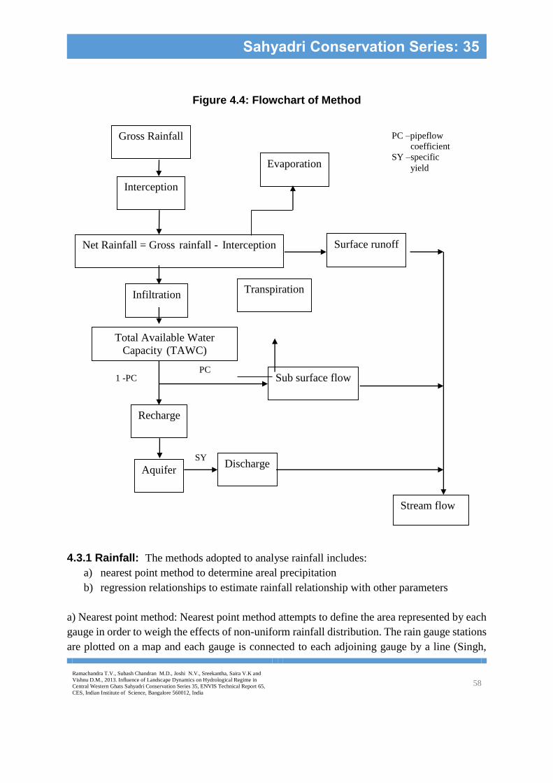
Ramachandra T.V., Subash Chandran M.D., Joshi N.V., Sreekantha, Saira V.K and
Vishnu D.M., 2013. Influence of Landscape Dynamics on Hydrological Regime in
Central Western Ghats Sahyadri Conservation Series 35, ENVIS Technical Report 65,
CES, Indian Institute of Science, Bangalore 560012, India 58
Sahyadri Conservation Series: 35
Figure 4.4: Flowchart of Method
4.3.1 Rainfall: The methods adopted to analyse rainfall includes:
a) nearest point method to determine areal precipitation
b) regression relationships to estimate rainfall relationship with other parameters
a) Nearest point method: Nearest point method attempts to define the area represented by each
gauge in order to weigh the effects of non-uniform rainfall distribution. The rain gauge stations
are plotted on a map and each gauge is connected to each adjoining gauge by a line (Singh,
Gross Rainfall
Interception
Net Rainfall = Gross rainfall - Interception Surface runoff
Infiltration
Sub surface flow
Recharge
Total Available Water
Capacity (TAWC)
Aquifer
Evaporation
Transpiration
Discharge
Stream flow
PC –pipeflow
coefficient
SY –specific
yield
1 -PC PC
SY

Ramachandra T.V., Subash Chandran M.D., Joshi N.V., Sreekantha, Saira V.K and
Vishnu D.M., 2013. Influence of Landscape Dynamics on Hydrological Regime in
Central Western Ghats Sahyadri Conservation Series 35, ENVIS Technical Report 65,
CES, Indian Institute of Science, Bangalore 560012, India 59
Sahyadri Conservation Series: 35
1992). Perpendicular bisectors of these connecting lines are drawn to form a polygon around
each gauge. The area within each polygon is assumed to be represented by each gauge. This
percent area of a gauge defines its weighting factor Ai, i =1,2,3….n. It is given by the equation
P = A
APAPAP nn .........221 (4.3)
where
P1,P2..Pn- precipitation (mm)
A1,A2,…..An-area enclosed by each polygon
A-total area
The weighted average rainfall for the drainage basin is computed by multiplying the rainfall at
each station by its assigned area within the drainage basin, represented by the polygon area
divided by the total drainage area and totaling the values.
b) Stepwise regression analysis was carried out for each rain gauge station considering rainfall
as dependent variable and latitude, longitude, altitude and land cover as probable independent
variables.
R = f(land cover, latitude, longitude and altitude) (4.4)
i.e. R = a1(land cover) a2(latitude) a3(longitude) a4(altitude) constant (4.5)
where a1, a2, a3, a4 – constants or coefficients of regression
4.3.2 Interception: Interception is considered as a function of canopy storage capacity C
and evaporative fraction () (Singh, 1992) and is given by the equation:
PCI (4.6)
The rate of evaporation of intercepted water from a wet canopy commonly exceeds the potential
evaporation for open water surfaces and indeed often the energy locally available to support it
(Shuttleworth, 1993). The additional energy is withdrawn from the atmosphere from warmer,
drier wind upward. The net amount of water, which the canopy can store, i.e. the interception
storage capacity, depends partly on the nature of rainfall, in particular the intensity and duration
of the rainstorm since upto half the evaporation occurs during the storm itself. For forests with
complete canopy cover, intense, short-lived, convective storms, more common in tropical
Ramachandra T.V., Subash Chandran M.D., Joshi N.V., Sreekantha, Saira V.K and
Vishnu D.M., 2013. Influence of Landscape Dynamics on Hydrological Regime in
Central Western Ghats Sahyadri Conservation Series 35, ENVIS Technical Report 65,
CES, Indian Institute of Science, Bangalore 560012, India 60
Sahyadri Conservation Series: 35
regions are associated with a lower fractional interception loss or evaporative fraction, say 10-
18 percent of precipitation (Lloyd et al., 1988; Shuttleworth, 1989). Storms associated with
frontal rainfall, which may be less intense but lasts longer tend to give a higher fractional
interception loss of say 20-30 percent of precipitation (Calder and Newson, 1979; Gash et al.,
1980). Table 4.3 lists the canopy storage capacities and evaporative fraction for different
vegetation types in the study area.
The following assumptions have been made for interception loss under each vegetation type in
upstream river basin. Major portion of the rainfall is received from the southwest monsoon,
which is of low intensity and longer duration. Thus, the evaporative fraction is considered
similar to that of frontal precipitation. Table 4.3 gives the interception characteristics of
different vegetation types. Table 4.4 lists the equations for each vegetation types following the
assumptions.
Assumptions
Evergreen/semievergreen forests
Dominated by evergreen trees
Leaves all year around- high storage capacity
Thick and multi layered canopy- higher evaporative fraction
Moist deciduous forests
Dominated by deciduous trees
Full leaves during monsoon season- maximum storage capacity
Large leaves- higher evaporative fraction
Plantations
Dominated by monoculture trees
Full leaves during monsoon season- maximum storage capacity
Narrow and vertically aligned leaves- lower evaporative fraction
Agricultural crops
Young leaves (July-August)- lower storage capacity and evaporative fraction
Mature leaves (September)- higher storage capacity and evaporative fraction
Grasslands and scrubs
Fully grown grass and scrubs-(June-September)- higher storage capacity and
evaporative fraction
Dry grass and scrubs (October)-lower storage capacity and evaporative fraction

Ramachandra T.V., Subash Chandran M.D., Joshi N.V., Sreekantha, Saira V.K and
Vishnu D.M., 2013. Influence of Landscape Dynamics on Hydrological Regime in
Central Western Ghats Sahyadri Conservation Series 35, ENVIS Technical Report 65,
CES, Indian Institute of Science, Bangalore 560012, India 61
Sahyadri Conservation Series: 35
Table 4.3: Interception Characteristics of Western Ghats
Vegetation types * Canopy storage
capacity (C) (mm) **Evaporative fraction ()
or net interception loss (%)
Evergreen/semievergreen 4.5-5.5 20-30
Moist deciduous forests 4-5 20-30
Plantations 4-5 20-30
Grasslands and scrubs 2.5-3.5 10-18
Agricultural crops (paddy) 1.8-2 10-18
*Source: Putty and Prasad, 2000
** Source: Modified evaporative fraction from Shuttleworth, 1993.
Table 4.4: Interception Equations for Upstream River Basin
Vegetation types Period Interception
Evergreen/semievergreen forests June-October I = 5.5 + 0.3 (P)
Moist deciduous forests June-October I = 5 + 0.3 (P)
Plantations June-October I = 5 + 0.2 (P)
Agricultural crops (paddy) June 0
July-August I = 1.8+ 0.1 (P)
September I = 2 + .18 (P)
October 0
Grasslands and scrubs June-September I = 3.5 +0.18 (P)
October I = 2.5 + 0.1 (P)
4.3.3 Surface Runoff
Surface runoff has been determined by rational method, which assumes a suitable runoff
coefficient to determine the catchment yield. It is given by the formula,
Yield= C*A*P (4.7)
where,
A-area of catchment/basin (km2)
P-precipitation in mm
C-runoff coefficient
Table 4.5 gives the runoff characteristics under each land cover type in the study area. The
following assumptions have been made.
Agricultural lands
Fallow period – high runoff
Crop growing period- low runoff
Grasslands and scrubs

Ramachandra T.V., Subash Chandran M.D., Joshi N.V., Sreekantha, Saira V.K and
Vishnu D.M., 2013. Influence of Landscape Dynamics on Hydrological Regime in
Central Western Ghats Sahyadri Conservation Series 35, ENVIS Technical Report 65,
CES, Indian Institute of Science, Bangalore 560012, India 62
Sahyadri Conservation Series: 35
Monsoon season- low runoff
Non monsoon season –high runoff
Table 4.5: Runoff Equations for Upstream River Basin
Land use/land cover Period C Runoff
Evergreen/semievergreen forests June-Oct 0.2 R = 0.2 *A*P
Moist deciduous forests June-Oct 0.2 R = 0.2 *A*P
Plantations June-Oct 0.2 R = 0.2 *A*P
Grasslands and scrubs June-Sept 0.3 R = 0.3 *A*P
Oct 0.6 R= 0.6 *A*P
Agricultural lands (paddy) June 0.6 R= 0.6 *A*P
July-Sept 0.4 R = 0.4 *A*P
Oct 0.6 R= 0.6 *A*P
Settlements June-Oct 0.8 R = 0.8 *A*P
Open fields June-Oct 0.6 R = 0.6 *A*P
4.3.4 Sub Surface Runoff (Pipeflow)
Sub surface runoff is considered to be the fraction of water that remains after infiltrated water
satisfies the available water capacities under each soil. The available water capacity (AWC)
for each soil texture is given in Table 4.6.
Table 4.6: Available Water Capacity
Soil texture AWC(%)
Loamy sand 9
Sandy clay loam 10
Clay loam with sand 10
Clay with sand 15
Source: http://soils.usda.gov/sqi/files/avwater.pdf
The total available water capacities (TAWC) under each land cover type in the study area are
given in Table 4.7.
Table 4.7: Total Available Water Capacity
Cover type Soil texture TAWC (%)
Evergreen/semievergreen forests Sandy clay loam 39
Clay loam with sand 40
Clay with sand 45
Loamy sand 64
Moist deciduous forests Sandy clay loam 45
Clay loam with sand 35
Clay with sand 45
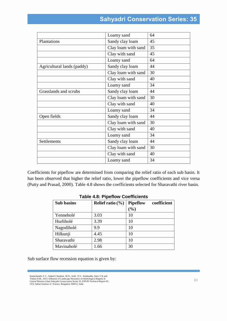
Ramachandra T.V., Subash Chandran M.D., Joshi N.V., Sreekantha, Saira V.K and
Vishnu D.M., 2013. Influence of Landscape Dynamics on Hydrological Regime in
Central Western Ghats Sahyadri Conservation Series 35, ENVIS Technical Report 65,
CES, Indian Institute of Science, Bangalore 560012, India 63
Sahyadri Conservation Series: 35
Loamy sand 64
Plantations Sandy clay loam 45
Clay loam with sand 35
Clay with sand 45
Loamy sand 64
Agricultural lands (paddy) Sandy clay loam 44
Clay loam with sand 30
Clay with sand 40
Loamy sand 34
Grasslands and scrubs Sandy clay loam 44
Clay loam with sand 30
Clay with sand 40
Loamy sand 34
Open fields Sandy clay loam 44
Clay loam with sand 30
Clay with sand 40
Loamy sand 34
Settlements Sandy clay loam 44
Clay loam with sand 30
Clay with sand 40
Loamy sand 34
Coefficients for pipeflow are determined from comparing the relief ratio of each sub basin. It
has been observed that higher the relief ratio, lower the pipeflow coefficients and vice versa
(Putty and Prasad, 2000). Table 4.8 shows the coefficients selected for Sharavathi river basin.
Table 4.8: Pipeflow Coefficients
Sub basins Relief ratio (%) Pipeflow coefficient
(%)
Yenneholé 3.03 10
Hurliholé 3.39 10
Nagodiholé 9.9 10
Hilkunji 4.45 10
Sharavathi 2.98 10
Mavinaholé 1.66 30
Sub surface flow recession equation is given by:
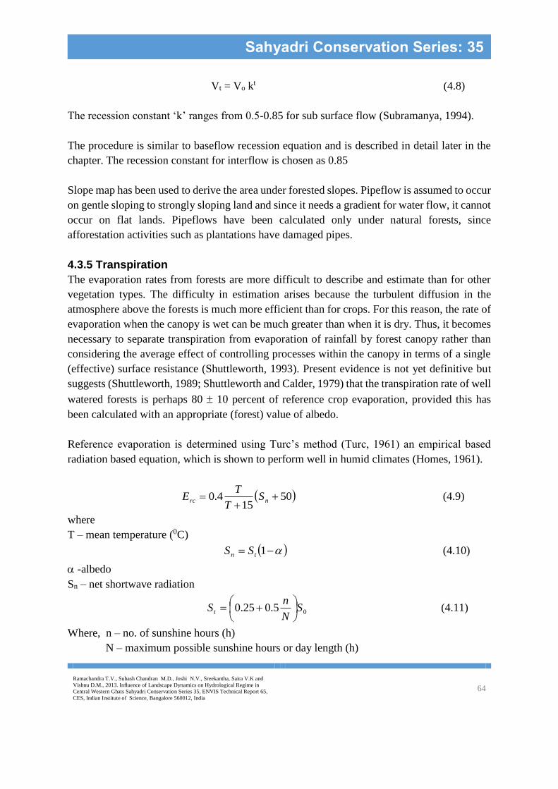
Ramachandra T.V., Subash Chandran M.D., Joshi N.V., Sreekantha, Saira V.K and
Vishnu D.M., 2013. Influence of Landscape Dynamics on Hydrological Regime in
Central Western Ghats Sahyadri Conservation Series 35, ENVIS Technical Report 65,
CES, Indian Institute of Science, Bangalore 560012, India 64
Sahyadri Conservation Series: 35
Vt = Vo kt (4.8)
The recession constant ‘k’ ranges from 0.5-0.85 for sub surface flow (Subramanya, 1994).
The procedure is similar to baseflow recession equation and is described in detail later in the
chapter. The recession constant for interflow is chosen as 0.85
Slope map has been used to derive the area under forested slopes. Pipeflow is assumed to occur
on gentle sloping to strongly sloping land and since it needs a gradient for water flow, it cannot
occur on flat lands. Pipeflows have been calculated only under natural forests, since
afforestation activities such as plantations have damaged pipes.
4.3.5 Transpiration
The evaporation rates from forests are more difficult to describe and estimate than for other
vegetation types. The difficulty in estimation arises because the turbulent diffusion in the
atmosphere above the forests is much more efficient than for crops. For this reason, the rate of
evaporation when the canopy is wet can be much greater than when it is dry. Thus, it becomes
necessary to separate transpiration from evaporation of rainfall by forest canopy rather than
considering the average effect of controlling processes within the canopy in terms of a single
(effective) surface resistance (Shuttleworth, 1993). Present evidence is not yet definitive but
suggests (Shuttleworth, 1989; Shuttleworth and Calder, 1979) that the transpiration rate of well
watered forests is perhaps 80 10 percent of reference crop evaporation, provided this has
been calculated with an appropriate (forest) value of albedo.
Reference evaporation is determined using Turc’s method (Turc, 1961) an empirical based
radiation based equation, which is shown to perform well in humid climates (Homes, 1961).
5015
4.0
nrc ST
TE (4.9)
where
T – mean temperature (0C)
1tn SS (4.10)
-albedo
Sn – net shortwave radiation
05.025.0 SN
nS t
(4.11)
Where, n – no. of sunshine hours (h)
N – maximum possible sunshine hours or day length (h)

Ramachandra T.V., Subash Chandran M.D., Joshi N.V., Sreekantha, Saira V.K and
Vishnu D.M., 2013. Influence of Landscape Dynamics on Hydrological Regime in
Central Western Ghats Sahyadri Conservation Series 35, ENVIS Technical Report 65,
CES, Indian Institute of Science, Bangalore 560012, India 65
Sahyadri Conservation Series: 35
So – extra terrestrial radiation (MJ/m2/day)
-latent heat of vapourisation of water (2.501 MJ/kg)
w- density of water ( 1000 kg/m3)
Thus, transpiration from forests is given by the equation
Eforest = (0.80.1) Erc (4.12)
Crop Transpiration
Crop transpiration is computed considering crop coefficient with reference crop evaporation
and is given by the equation
E = Kc Erc (4.13)
where, Erc- reference crop evaporation
Kc – crop coefficient (grasses = 0.8)
The following assumptions have been made in the selection of albedo values for reference crop
evaporation under each vegetation type based on the months and season in the study area.
Assumptions
Evergreen/semievergreen forests
Dominated by evergreen trees
Leaves all year around- low albedo
Moist deciduous forests
Clear felled with secondary vegetation (albedo increased by 0.02) (Dickinson, 1980)
Dominated by deciduous trees
Full leaves during monsoon season- low albedo
Non monsoon season-high albedo
Plantations
Mostly deciduous trees eg. acacia, eucalyptus
Plantation is considered to be more open than an intact evergreen or moist deciduous
forests and hence the albedo is increased by 0.03.
Full leaves during monsoon season- low albedo
Non monsoon season-high albedo
Agricultural crops
Fallow period- high albedo
Crop growing period (young leaves)-high albedo
Mature crops-low albedo
Paddy is assumed to grow during July-September considering it as a 90 days crop

Ramachandra T.V., Subash Chandran M.D., Joshi N.V., Sreekantha, Saira V.K and
Vishnu D.M., 2013. Influence of Landscape Dynamics on Hydrological Regime in
Central Western Ghats Sahyadri Conservation Series 35, ENVIS Technical Report 65,
CES, Indian Institute of Science, Bangalore 560012, India 66
Sahyadri Conservation Series: 35
Grasslands and scrubs
Monsoon season (June-September)- low albedo
Non monsoon (dry grass)(October)-high albedo
Table 4.9 lists the albedo values selected for vegetation according to months.
Table 4.9: Albedo Values for Vegetation
Vegetation types Albedo Range Albedo Period
Evergreen forests 0.11-0.16 0.11 Jan-Dec
Moist deciduous forests 0.11-0.16 0.13* May-October
0.16 November-April
Plantations 0.11-0.16 0.14* May-October
0.16 November-April
Grasslands and scrubs 0.20-0.26 0.20 June-September
0.26 October-May
Agricultural land (paddy) 0.20-0.26 0.08 June
0.20 July-August
0.26 September
0.08 October
Source: Shuttleworth,1993 in Handbook of Hydrology
* Dickinson, 1980
4.3.6 Evaporation
Turc’s method is used to estimate evporation from soil and open water with the appropriate
albedo values. Table 4.10 lists the albedo values selected for other land covers.
Open field and settlements
Monsoon season- low albedo
Non monsoon season- high albedo
Table 4.10: Albedo Values for Other land covers
Cover type Albedo range Albedo Period
Open water 0.08 0.08 Jan-Dec
Open fields 0.1-0.35 0.1 June-October
0.35 November-May
Settlements 0.1-0.35 0.1 June-October
0.35 November-May
Source: Shuttleworth, 1993

Ramachandra T.V., Subash Chandran M.D., Joshi N.V., Sreekantha, Saira V.K and
Vishnu D.M., 2013. Influence of Landscape Dynamics on Hydrological Regime in
Central Western Ghats Sahyadri Conservation Series 35, ENVIS Technical Report 65,
CES, Indian Institute of Science, Bangalore 560012, India 67
Sahyadri Conservation Series: 35
4.3.7 Groundwater Recharge
Recharge is considered the fraction of infiltrated water that recharges the aquifer after
satisfying available water capacity and pipe flow.
4.3.8 Groundwater Discharge
Groundwater discharge or base flow is estimated by multiplying the average specific yield of
aquifer under each land cover with the recharged water. Specific yield represents the water
yielded from water bearing material. In other words, it is the ratio of the volume of water that
the material, after being saturated, will yield by gravity to its own volume. Base flow appears
after monsoon and pipe flow has receded. This water sustains flow in the rivers during the dry
season. Groundwater storage-discharge is considered to be linear after Maillet (1905) since it
is widely used following tradition and due to the ease of mathematical manipulation
(Wittenburg and Sivapalan, 1999). The exponential function has been widely used to describe
base flow recession, where Qt is discharge at time ‘t’ and Q0 is the initial discharge and a is a
recession constant. The exponential function describes that the groundwater aquifer behaves
like a single linear reservoir with storage linearly proportional to outflow i.e.
S =a Q (4.14)
This equation represents a first order process or an exhaustion phenomenon expressed by
Qdt
ds (4.15)
Q(0)= Q0
The most widely used base flow recession equations are of the exponential forms such as
Equation 4.16 by Barnes, (1939).
Qt = Q0 kt (4.16)
where, Q0- initial discharge
k – base flow recession constant (0.85-0.99) (Subramanya, 1994).
t - time
In the absence of discharge data, volumes can be used. Replacing discharge with volume does
not change its form and is less sensitive to errors than when using discharge data (Singh, 1992).
Shirmohammadi et al. (1984) used volumes for partitioning stream flow data in surface and
sub surface flows.
Groundwater volume at any time ‘t’ is determined by the equation :
Vt = Vo k t (4.17)

Ramachandra T.V., Subash Chandran M.D., Joshi N.V., Sreekantha, Saira V.K and
Vishnu D.M., 2013. Influence of Landscape Dynamics on Hydrological Regime in
Central Western Ghats Sahyadri Conservation Series 35, ENVIS Technical Report 65,
CES, Indian Institute of Science, Bangalore 560012, India 68
Sahyadri Conservation Series: 35
Assumptions
The entire river basin is considered to be an unconfined aquifer
Base flow recession constant is assumed to be 0.95
Table 4.11 gives the average specific yields of each sub basin.
Table 4.11: Average Specific Yields of Sub basins
Sub basins Rock type (French Soil Map) Avg. Specific yield (%)
Yenneholé Gneisses/granites
Greywackes
15
Nagodiholé Greywackes 27
Hurliholé Gneisses/granites
Greywackes
15
Hilkunji Gneisses/granites
Greywackes
15
Sharavathi Gneisses/granites
Greywackes
15
Linganamakki Gneisses/granites
Greywackes
15
Mavinaholé Gneisses/granites 3
Haridravathi Gneisses/granites 3
Nandiholé Gneisses/granites 3

Ramachandra T.V., Subash Chandran M.D., Joshi N.V., Sreekantha, Saira V.K and
Vishnu D.M., 2013. Influence of Landscape Dynamics on Hydrological Regime in
Central Western Ghats Sahyadri Conservation Series 35, ENVIS Technical Report 65,
CES, Indian Institute of Science, Bangalore 560012, India 69
Sahyadri Conservation Series: 35
5.0 Results and Discussions Analysis was carried out for different hydrological components using the methods described
earlier.
5.1 Land use dynamics:
Figure 5.1: Reserve Forest Area (1940)
Table 5.1 gives the percentage forest cover (reserved forests) derived from 1940 toposheets
(48K/13, 48J/16 and 48O/1), 1989 (Landsat TM) and 1999 (LISS III) imageries. More than
50% of the forests have decreased/removed by human activities and submergence due to
damming the Sharavathi River.
Table 5.1: Changes in Reserve Forests Area (1940-1999)
1940 (sq.km) 1989 (sq.km) 1999 (sq.km) Change in % (1935-1999)
185.09 99.46 89.73 -51.52%
Land use/Land cover maps of Sharavathi river basin (upstream) for 1989 and 1999 are given
in Figure 5.2 and 5.3

Ramachandra T.V., Subash Chandran M.D., Joshi N.V., Sreekantha, Saira V.K and
Vishnu D.M., 2013. Influence of Landscape Dynamics on Hydrological Regime in
Central Western Ghats Sahyadri Conservation Series 35, ENVIS Technical Report 65,
CES, Indian Institute of Science, Bangalore 560012, India 70
Sahyadri Conservation Series: 35
Figure 5.2: Land use Classification (Landsat TM, 1989)
Figure 5.3: Land use Classification (IRS LISS III, 1999)
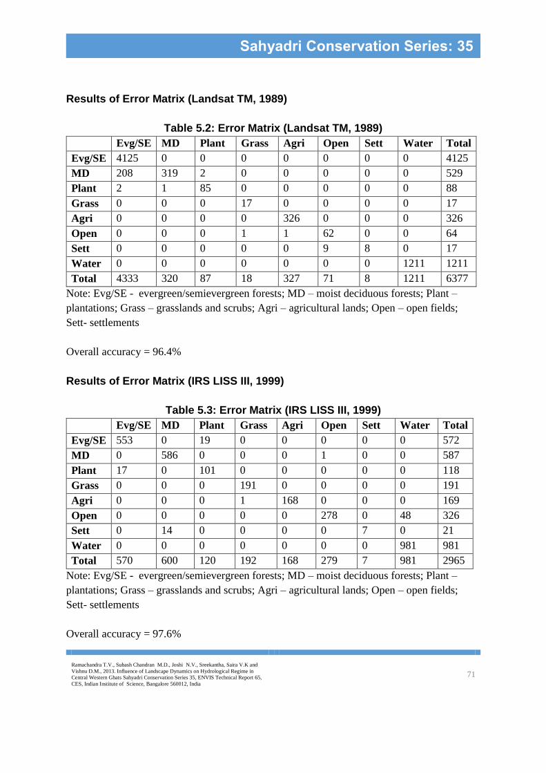
Ramachandra T.V., Subash Chandran M.D., Joshi N.V., Sreekantha, Saira V.K and
Vishnu D.M., 2013. Influence of Landscape Dynamics on Hydrological Regime in
Central Western Ghats Sahyadri Conservation Series 35, ENVIS Technical Report 65,
CES, Indian Institute of Science, Bangalore 560012, India 71
Sahyadri Conservation Series: 35
Results of Error Matrix (Landsat TM, 1989)
Table 5.2: Error Matrix (Landsat TM, 1989)
Evg/SE MD Plant Grass Agri Open Sett Water Total
Evg/SE 4125 0 0 0 0 0 0 0 4125
MD 208 319 2 0 0 0 0 0 529
Plant 2 1 85 0 0 0 0 0 88
Grass 0 0 0 17 0 0 0 0 17
Agri 0 0 0 0 326 0 0 0 326
Open 0 0 0 1 1 62 0 0 64
Sett 0 0 0 0 0 9 8 0 17
Water 0 0 0 0 0 0 0 1211 1211
Total 4333 320 87 18 327 71 8 1211 6377
Note: Evg/SE - evergreen/semievergreen forests; MD – moist deciduous forests; Plant –
plantations; Grass – grasslands and scrubs; Agri – agricultural lands; Open – open fields;
Sett- settlements
Overall accuracy = 96.4%
Results of Error Matrix (IRS LISS III, 1999)
Table 5.3: Error Matrix (IRS LISS III, 1999)
Evg/SE MD Plant Grass Agri Open Sett Water Total
Evg/SE 553 0 19 0 0 0 0 0 572
MD 0 586 0 0 0 1 0 0 587
Plant 17 0 101 0 0 0 0 0 118
Grass 0 0 0 191 0 0 0 0 191
Agri 0 0 0 1 168 0 0 0 169
Open 0 0 0 0 0 278 0 48 326
Sett 0 14 0 0 0 0 7 0 21
Water 0 0 0 0 0 0 0 981 981
Total 570 600 120 192 168 279 7 981 2965
Note: Evg/SE - evergreen/semievergreen forests; MD – moist deciduous forests; Plant –
plantations; Grass – grasslands and scrubs; Agri – agricultural lands; Open – open fields;
Sett- settlements
Overall accuracy = 97.6%

Ramachandra T.V., Subash Chandran M.D., Joshi N.V., Sreekantha, Saira V.K and
Vishnu D.M., 2013. Influence of Landscape Dynamics on Hydrological Regime in
Central Western Ghats Sahyadri Conservation Series 35, ENVIS Technical Report 65,
CES, Indian Institute of Science, Bangalore 560012, India 72
Sahyadri Conservation Series: 35
Low accuracy for settlements from both the imageries is partly due to spectral signature overlap
with vegetation as most of the houses are surrounded by vegetation inside and outside the
compound. Townships are few and houses are sparsely distributed separated by hundreds of
meters. Since the building material is also different as almost all houses have tiled roof than
concrete, overlap also occurred between open fields. Overlap of spectral signatures was also
observed between evergreen/semievergreen forest and moist deciduous forests in full leaf.
Table 5.4 compares the percentage change in the land use in Sharavathi upstream river basin.
Table 5.4: Changes in Land use in Upstream (1989-1999)
Land use/Land cover 1989 (km2) 1990 (km2) Change in %
Evergreen/semievergreen
forests
272.67 209.39 - 23.2
Moist deciduous forests 539.26 512.25 - 5
Plantations 122.09 143.29 +17.3
Grasslands and scrubs 433.98 310.6 - 28.4
Agricultural lands 102.77 157.36 + 53.1
Open fields/Barren lands 247.96 430.29 + 73.5
Settlements 52.63 78.48 + 49.1
Water bodies 218.01 147.31 -32.4
From Table 5.4, it is seen that natural forests such as evergreen/semi-evergreen and moist
deciduous forests have decreased by 28.2% whereas monoculture plantations (due to
afforestation work of the forest department) have increased by 17.3%. Grasslands and scrubs
have decreased by 28.4% in 1999 but this can be attributed to the season as in summer, grasses
dry out leaving only the scrubs. The main anthropogenic activity apart from plantation is paddy
cultivation, which has increased by 5% in 1999. Paddy cultivation is the most common
agricultural activity in the basin and is usually grown in valleys. Shimoga ranks first among
the other districts of the state as far as paddy is concerned (KSG, 1975).
Human population has also increased in the basin and has been reported that there has been
immigration of people from adjoining districts of Karnataka and also from neighbouring States
(KSG, 1975). In recent years, few people from drought affected districts of Gulbarga and Bidar
to Shimoga district to work on daily wages. A large number of seasonal in-migrants visit the
villages at different seasons of the year. They arrive in large numbers in October-November
and continue to stay there upto the end of about February-March. Some factory workers from
Bhadravati town also come to villages to work on the agricultural lands during peak harvesting
season.

Ramachandra T.V., Subash Chandran M.D., Joshi N.V., Sreekantha, Saira V.K and
Vishnu D.M., 2013. Influence of Landscape Dynamics on Hydrological Regime in
Central Western Ghats Sahyadri Conservation Series 35, ENVIS Technical Report 65,
CES, Indian Institute of Science, Bangalore 560012, India 73
Sahyadri Conservation Series: 35
Another major activity that has been beneficial to the villages in Sharavathi and also adjoining
districts is the setting up of the Linganamakki Dam across the Sharavathi River. The Sharavathi
Hydroelectric Project formerly known as Honnemaradu Project was taken up by the State
Government in 1956, to utilize the potential of the river. It has been one of the important
undertakings of the state in the field of economic development (KSG, 1975). A dam of nearly
2.4 kms long has been put across this river at Linganamakki in Sagar taluk of Shimoga district.
It was so designed as to impound 4368 million cubic meter of water in an area of around 300
km2, submerging 50.62 km2 of wetland, 7 km2 of dry land and 3.9 km2, the remaining being
forest land and wasteland.
Although the dam has provided electricity, water and other benefits to the surrounding areas,
it has proved to be at the cost of the valuable ecosystem. Evergreen forests are being cleared to
yield timber, which are used for electric transmission poles and railway sleepers. The felled
areas are sometimes tended for getting the natural regeneration of valuable species. Deciduous
forests supply timber, firewood, charcoal, bamboo, matchwood and plywood. Plantations of
teak, silver oak (Gravillea robusta), matchwood etc are sometimes replaced for clear felled
forests.
Table 5.5 and Table 5.6 give the sub-basin wise area under different land uses. Table 5.7 gives
the overall change in 1999.
Note: Evg/SE - evergreen/semievergreen forests; MD – moist deciduous forests; Plant –
plantations; Grass – grasslands and scrubs; Agri – agricultural lands; Open – open fields;
Sett- settlements
Table 5.5: Area of Land use in Sub Basins (sq.km)
1989
Sub Basins Evg/SE MD Plant Grass Agri Open Sett
Yenneholé 50.78 59.21 12.87 34.51 3.86 26.66 4.01
Nagodiholé 25.13 19.26 6.62 7.59 0.07 4.67 0.61
Hurliholé 24.88 31.73 8.3 17.55 1.52 9.95 1.47
Linganamakki 88.25 187.76 43.31 149.01 42.32 89.83 20.73
Hilkunji 24.59 25.41 5.1 14.35 4.041 10.69 1.84
Sharavathi 21.67 34.32 9.9 39.47 6.94 22.81 4.25
Mavinaholé 10.75 38.09 7.17 23.39 3.84 10.05 1.57
Haridravathi 15.85 74.47 16.79 101.21 28.36 48.32 12.68
Nandiholé 10.37 67.96 11.54 46.33 10.97 24.5 5.33

Ramachandra T.V., Subash Chandran M.D., Joshi N.V., Sreekantha, Saira V.K and
Vishnu D.M., 2013. Influence of Landscape Dynamics on Hydrological Regime in
Central Western Ghats Sahyadri Conservation Series 35, ENVIS Technical Report 65,
CES, Indian Institute of Science, Bangalore 560012, India 74
Sahyadri Conservation Series: 35
Table 5.6 Area of Land use in Sub Basins (sq.km)
1999
Sub Basins Evg/SE MD Plant Grass Agri Open Sett
Yenneholé 54.22 45.52 29.27 22.82 2.07 38.5 6.05
Nagodiholé 26.17 15.21 8.87 3.09 .03 8.42 2.81
Hurliholé 22.14 30.45 7.99 13.37 1.24 18.26 3.08
Linganamakki 50.47 202.38 55.41 13.37 50.47 194.91 25.72
Hilkunji 25.79 30.02 5.57 6.53 4.94 9.9 3.67
Sharavathi 16.29 40.66 14.16 16.35 19.37 27.31 7.06
Mavinaholé 2.36 33.9 4.87 20.47 10.3 18.08 6.62
Haridravathi 3.87 64.87 11.65 79.9 49.93 73.39 14.34
Nandiholé 2.22 48.48 5.19 52.71 18.71 41.03 8.96
Table 5.7: Changes in Land use in Sub Basins sq.km
1999
Sub Basins Evg/SE MD Plant Grass Agri Open Sett
Yenneholé 3.44 -13.69 16.4 -11.69 -1.79 11.84 2.04
Nagodiholé 1.04 -4.05 2.25 -4.5 -0.04 3.75 2.2
Hurliholé -2.74 -1.28 -0.31 -4.18 -0.28 8.31 1.61
Linganamakki -37.78 14.62 12.1 -135.64 8.15 105.08 4.99
Hilkunji 1.2 4.61 0.47 -7.82 0.89 -0.79 1.83
Sharavathi -5.38 6.34 4.26 -23.12 12.43 4.5 2.81
Mavinaholé -8.39 -4.19 -2.3 -2.92 6.46 8.03 5.05
Haridravathi -11.98 -9.6 -5.14 -21.31 21.57 25.07 1.66
Nandiholé -8.15 -19.48 -6.35 6.38 7.74 16.53 3.63
5.2 Rainfall
i) Talukwise rainfall analysis
Yearly data for hundred years were available for 7 taluks in and around the river basin viz.
Hosanagara, Sagara, Soraba and Tirthahalli (Shimoga district) and Honnavar, Kumta and
Siddapur (Uttara Kannada district). Since these are the taluks surrounding the river basin,
rainfall analysis is done to study any variation in rainfall for 100 years. The rainfall periods
were divided into 1901-1964 and 1964-2001, which represents respectively the periods before
construction and after construction of Linganamakki dam.

Ramachandra T.V., Subash Chandran M.D., Joshi N.V., Sreekantha, Saira V.K and
Vishnu D.M., 2013. Influence of Landscape Dynamics on Hydrological Regime in
Central Western Ghats Sahyadri Conservation Series 35, ENVIS Technical Report 65,
CES, Indian Institute of Science, Bangalore 560012, India 75
Sahyadri Conservation Series: 35
The graphs depict the rainfall variation in all taluks for the 2 periods. The highest rainfalls in
Hosanagara occured in 1961 and 1994 with 5175 mm and 5110 mm respectively. Sagara
experienced high rainfall of 4826 mm in 1962 and low rainfall of 993m in 1976. Low rainfall
was also recorded in Soraba consecutively for 4 years during 1979-1982 with the lowest
recorded in 2001. Tirthahalli recorded maximum rainfalls of 6400 and 6115 during the first
period (1901-1963) and a maximum rainfall of 4044 during the second period (1965-2001).
Analysis of 100 years rainfall in the various taluks in and around the river basin were done to
study any discrepancies in the rainfall for two periods viz. 1901-1964 (before construction of
dam) and 1964-2001 (after construction of dam).
Figure 5.4: Annual rainfall (Hosanagara) Figure 5.5: Annual rainfall
(Sagara)
Figure 5.6: Annual rainfall (Soraba) Figure 5.7: Annual rainfall (Tirthahalli)
Figure5.8: Annual rainfall (Honnavar) Figure5.9: Annual rainfall (Kumta)
Mean annual rainfall (1901-2001)
Soraba
0
1000
2000
3000
4000
1902 1913 1924 1934 1944 1955 1966 1976 1986 1996
Time
Rain
fall
in
mm
Mean annual rainfall (1901-2001)
Tirthahalli
0
1000
2000
3000
4000
5000
6000
7000
1901
1907
1913
1919
1925
1931
1937
1943
1949
1956
1962
1970
1976
1982
1988
1994
2000
Time
Rain
fall
in
mm
Mean annual rainfall (1901-2001)
Honnavar
0
1000
2000
3000
4000
5000
6000
1901 1911 1947 1959 1971 1981 1991 2001
Time
Rain
fall
in
mm
Mean annual rainfall (1901-2001)
Kumta
0
1000
2000
3000
4000
5000
6000
7000
1901 1911 1921 1931 1941 1951 1965 1975 1985 1995
Time
Rain
fall
in
mm
Annual rainfall(1901-2001)
Hosanagara
0
1000
2000
3000
4000
5000
6000
1901 1914 1924 1934 1945 1958 1970 1980 1990 2000
Year
Rain
fall
in
mm
Annual rainfall(1901-2001)
Sagara
0
1000
2000
3000
4000
5000
6000
1901 1912 1922 1932 1942 1953 1964 1975 1985 1995
Year
Ra
infa
ll in
mm

Ramachandra T.V., Subash Chandran M.D., Joshi N.V., Sreekantha, Saira V.K and
Vishnu D.M., 2013. Influence of Landscape Dynamics on Hydrological Regime in
Central Western Ghats Sahyadri Conservation Series 35, ENVIS Technical Report 65,
CES, Indian Institute of Science, Bangalore 560012, India 76
Sahyadri Conservation Series: 35
Figure 5.10: Annual rainfall (Siddapur)
Figure 5.11: Mean annual rainfall Figure 5.12: Mean annual rainfall
(1901-1964) (Hosanagara) (1965-2001) (Hosanagara)
Figure 5.13: Mean annual rainfall Figure 5.14: Mean annual rainfall
(1901-1964) (Sagara) (1964-2001) (Sagara)
Figure 5.15: Mean annual rainfall Figure 5.16: Mean annual rainfall
(1901-1964) (Soraba) (1964-2001) (Soraba)
Mean annual rainfall (1901-2001)
Siddapur
0
1000
2000
3000
4000
5000
6000
7000
1901 1911 1921 1931 1941 1951 1962 1973 1984 1994
Time
Rain
fall
in
mm
Mean annual rainfall (1901-1964)
Sagara
0
1000
2000
3000
4000
5000
6000
1901 1912 1922 1932 1942 1953 1964
Time
Rain
fall
in
mm
Mean annaul rainfall (1965-2001)
Sagara
0
1000
2000
3000
4000
1965 1976 1986 1996
Time
Rain
fall
in
mm
Mean annual rainfall (1901-1964)
Soraba
0
1000
2000
3000
4000
1902 1913 1924 1934 1944 1955
Time
Rain
fall
in
mm
Mean annual rainfall (1965-2001)
Soraba
0
1000
2000
3000
1966 1976 1986 1996
Time
Rain
fall
in
mm
Mean annual rainfall (1901-1964)
Hosanagara
0
1000
2000
3000
4000
5000
6000
1901 1914 1924 1934 1945 1958
Time
Rain
fall
in
mm
Mean annual rainfall (1965-2001) Hosanagara
0
1000
2000
3000
4000
5000
6000
1965 1976 1986 1996Time
Rain
fall
in
mm

Ramachandra T.V., Subash Chandran M.D., Joshi N.V., Sreekantha, Saira V.K and
Vishnu D.M., 2013. Influence of Landscape Dynamics on Hydrological Regime in
Central Western Ghats Sahyadri Conservation Series 35, ENVIS Technical Report 65,
CES, Indian Institute of Science, Bangalore 560012, India 77
Sahyadri Conservation Series: 35
Figure 5.17: Mean annual rainfall Figure 5.18: Mean annual rainfall
(1901-1963) (Tirthahalli) (1965-2001) (Tirthahalli)
Figure 5.19: Mean annual rainfall Figure 5.20: Mean annual rainfall
(1901-1963)(Honnavar) (1965-2001)(Honnavar)
Figure 5.21: Mean annual rainfall Figure 5.22: Mean annual rainfall
(1901-1963) (Kumta) (1965-2001) (Kumta)
Figure 5.23: Mean annual rainfall Figure 5.24: Mean annual rainfall
(1901-1963) (Siddapur) (1963-2001) (Siddapur)
Mean annual rainfall (1901-1963)
Tirthahalli
0
1000
2000
3000
4000
5000
6000
7000
1901 1911 1921 1931 1941 1951 1962
Time
Rain
fall
in
mm
Mean annual rainfall (1965-2001)
Tirthahalli
0
1000
2000
3000
4000
5000
1965 1976 1986 1996
Time
Rain
fall
in
mm
Mean annual rainfall (1901 -1963)
Honnavar
0
1000
2000
3000
4000
5000
6000
1901
1904
1907
1910
1913
1941
1945
1948
1952
1956
1959
1963
Time
Rain
fall
in
mm
Mean annual rainfall (1965-2001)
Honnavar
0
1000
2000
3000
4000
5000
6000
1965
1968
1971
1974
1977
1980
1983
1986
1989
1992
1995
1998
2001
Time
Rain
fall
in
mm
Mean annual rainfall (1901-1963)
Kumta
0100020003000
4000500060007000
1901
1905
1909
1913
1917
1921
1925
1929
1933
1937
1941
1945
1949
1953
1958
Time
Rain
fall
in
mm
Mean annual rainfall (1965-2001)
Kumta
0
1000
2000
3000
4000
5000
1965
1968
1971
1974
1977
1980
1983
1986
1989
1992
1995
1998
2001
Time
Rain
fall
in
mm
Mean annual rainfall (1901-1963)
Siddapur
01000200030004000500060007000
1901
1905
1909
1913
1917
1921
1925
1929
1933
1937
1941
1945
1949
1953
1958
1962
Time
Rain
fall
in
mm
Mean annual rainfall (1963-2001)
Siddapur
0
1000
2000
3000
4000
5000
6000
1965
1968
1971
1974
1977
1980
1984
1987
1990
1993
1996
1999
Time
Rain
fall
in
mm

Ramachandra T.V., Subash Chandran M.D., Joshi N.V., Sreekantha, Saira V.K and
Vishnu D.M., 2013. Influence of Landscape Dynamics on Hydrological Regime in
Central Western Ghats Sahyadri Conservation Series 35, ENVIS Technical Report 65,
CES, Indian Institute of Science, Bangalore 560012, India 78
Sahyadri Conservation Series: 35
Table 5.8 gives the mean and standard deviation of rainfall in Shimoga district
Table 5.8: Variation of Rainfall in Shimoga
Taluk 1901-2001
(mm)
COV
(%)
1901-1964
(mm)
COV
(%)
1965-2001
(mm)
COV
(%)
Change in
rainfall
(%)
Hosanagara 2813.9
754.4
26.8 2854.2
683.4
23.9 2752.8
859.9
31.2 -3.55
Sagara 2098.1
523.6
24.9 2144.5
560.3
26.1 2018.4
444.2
22 -5
Soraba 1583.8
430.0
27.1 1627.3
388.6
23.8 1511.4
488.6
32.3 2.4
Tirthahalli 3051.8
783.6
25.6 *3132.9
841.4
26.8 2742.6
607.0
22.1 -12.45
* 1901-1963
Table 5.9 gives the mean and standard deviation of rainfall in Uttara Kannada district
Table 5.9: Variation of Rainfall in Uttara Kannada
Taluk 1901-2001
(mm)
COV
(%)
1901-1963
(mm)
COV
(%)
1965-2001
(mm)
COV
(%)
Change
in
rainfall
(%)
Honnavar 3485.1 687.8 19.7 3360.6
775.4
23 3636.3 565.5 15.55 8.2
Kumta 3755.9 750.7 19.9 3633.8
831.9
22.8 3391.1 575.3 16.9 -6
Siddapur 2999.8 769.9 25.6 3037 793.2 26.1 2935.6 734.4 25 -3.3
Hosanagara, Sagara, Tirthahalli and Siddapur taluks showed reduction in the mean annual
rainfall with a significant reduction in Tirthahalli taluk. Sagara and Hosanagara were selected
for further studies as these districts cover the study area. A student’s t test was carried out to
determine whether the changes in mean annual rainfall are significant for 2 periods viz. 1901-
1964 and 1964-2001. The test produced the following results.
Table 5.10: t Test for Rainfall Variation
Taluks T Degrees of
freedom
(df)
t0.95 t0.99
Hosanagara 0.00062 91 1.662 2.368
Sagara 1.3 96 1.61 2.366

Ramachandra T.V., Subash Chandran M.D., Joshi N.V., Sreekantha, Saira V.K and
Vishnu D.M., 2013. Influence of Landscape Dynamics on Hydrological Regime in
Central Western Ghats Sahyadri Conservation Series 35, ENVIS Technical Report 65,
CES, Indian Institute of Science, Bangalore 560012, India 79
Sahyadri Conservation Series: 35
Null hypothesis H0-no significant change in mean annual rainfall during the 2 periods
Alternative hypothesis H1-significant change in mean annual rainfall during the 2 periods
Hosanagara
At df=91, t0.05 = 1.662, i.e. 0.00062<1.662, null hypothesis is accepted
t0.01 = 2.368, i.e. 0.00062<2.368, null hypothesis is accepted
Sagara
At df=96, t0.05 = 1.61, i.e. 1.3 <1.662, null hypothesis is accepted
t0.01 = 2.366, i.e. 1.3<2.368, null hypothesis is accepted
At 0.05% and 0.01% the null hypothesis is accepted for both the taluks.
Coefficient of variation was also calculated for all taluks. Coefficient of variation (COV) is the
standard deviation divided by the mean. In practice, it “scales” the standard deviation by the
size of the mean, making it possible to compare coefficients of variation across variables
measured on different scales. Taluks in Shimoga district showed higher coefficient of
variations as compared to Uttara Kannada with the exception of Siddapur. High CV shows that
there is high rainfall variation from the mean rainfall. However, Hosanagara and Sagara
showed the highest rainfall variation during 1965-2001.
Mean monthly rainfalls show a reduction of 200 mm and 100 mm in July (peak rainfall month)
in Hosanagara and Sagara respectively.
ii) Mean monthly rainfall variation in Hosanagara and Sagara
Figure 5.25: Mean Monthly Rainfall of Sagara and Hosanagara
Mean monthly rainfall Hosanagara
1901-1964
0
200
400
600
800
1000
1200
Jan Feb Mar Apr May Jun Jul Aug Sep Oct Nov Dec
Year
Rain
fall
in
mm
Mean monthly rainfall Sagara
1901-1964
0
200
400
600
800
1000
Jan Feb Mar Apr May Jun Jul Aug Sep Oct Nov Dec
Months
Rain
fall
in
mm
Mean monthly rainfall Sagara
1964-2001
0
200
400
600
800
Jan Feb Mar Apr May Jun Jul Aug Sep Oct Nov Dec
Months
Rain
fall
in
mm
Mean monthly rainfall Hosanagara
1964-2001
0
200
400
600
800
1000
1200
Jan Feb Mar Apr May Jun Jul Aug Sep Oct Nov Dec
Months
Rain
fall
in
mm

Ramachandra T.V., Subash Chandran M.D., Joshi N.V., Sreekantha, Saira V.K and
Vishnu D.M., 2013. Influence of Landscape Dynamics on Hydrological Regime in
Central Western Ghats Sahyadri Conservation Series 35, ENVIS Technical Report 65,
CES, Indian Institute of Science, Bangalore 560012, India 80
Sahyadri Conservation Series: 35
The mean monthly variation shows that the bulk of the rainfall occurs in the months of June,
July and August. Rainfall peaks in the month of July and decreases then onwards with a slight
increase in October (beginning of northeast monsoon). Both Hosanagara and Sagara show
decrease in the peak rainfall month by 200 mm and 100 mm respectively during (1964-2001).
Table 5.11 compares the change in monthly rainfall for the two taluks.
Table 5.11: Changes in Mean Monthly Rainfall (Hosanagara and Sagara)
Taluks Mean rainfall in mm (June, July and August)
1901-1964 1965-2001 Change in %
Hosanagara 775.33 740.4 - 4.5%
Sagara 547.0 526.4 - 3.8%
iii) Sub-basin rainfall analysis
Rainfall data were available for 18 rain gauge stations from 1989-1999. Due to non-availability
of data for certain months, analysis is done with respect to 5 months viz. June, July, August,
September and October. Areal precipitation was determined for each sub basin and upstream.
Figure 5.26 depicts the rain gauges in upstream river basin.
Figure 5.26: Rain Gauges of Upstream
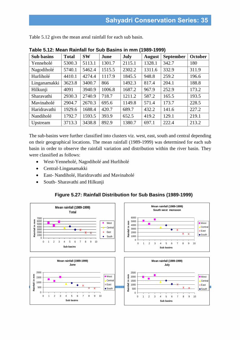
Ramachandra T.V., Subash Chandran M.D., Joshi N.V., Sreekantha, Saira V.K and
Vishnu D.M., 2013. Influence of Landscape Dynamics on Hydrological Regime in
Central Western Ghats Sahyadri Conservation Series 35, ENVIS Technical Report 65,
CES, Indian Institute of Science, Bangalore 560012, India 81
Sahyadri Conservation Series: 35
Table 5.12 gives the mean areal rainfall for each sub basin.
Table 5.12: Mean Rainfall for Sub Basins in mm (1989-1999)
Sub basins Total SW June July August September October
Yenneholé 5300.3 5113.1 1301.7 2115.1 1328.1 342.7 180
Nagodiholé 5740.1 5462.4 1515.5 2302.2 1311.6 332.9 311.9
Hurliholé 4410.1 4274.4 1117.9 1845.5 948.8 259.2 196.6
Linganamakki 3623.8 3400.7 866 1492.3 817.4 204.1 188.8
Hilkunji 4091 3940.9 1006.8 1687.2 967.9 252.9 173.2
Sharavathi 2930.3 2740.9 718.7 1211.2 587.2 165.5 193.5
Mavinaholé 2904.7 2670.3 695.6 1149.8 571.4 173.7 228.5
Haridravathi 1929.6 1688.4 420.7 689.7 432.2 141.6 227.2
Nandiholé 1792.7 1593.5 393.9 652.5 419.2 129.1 219.1
Upstream 3713.3 3438.8 892.9 1380.7 697.1 222.4 213.2
The sub-basins were further classified into clusters viz. west, east, south and central depending
on their geographical locations. The mean rainfall (1989-1999) was determined for each sub
basin in order to observe the rainfall variation and distribution within the river basin. They
were classified as follows:
West-Yenneholé, Nagodiholé and Hurliholé
Central-Linganamakki
East- Nandiholé, Haridravathi and Mavinaholé
South- Sharavathi and Hilkunji
Figure 5.27: Rainfall Distribution for Sub Basins (1989-1999)
Mean rainfall (1989-1999)
South west monsoon
0
1000
2000
3000
4000
5000
6000
0 1 2 3 4 5 6 7 8 9 10
Sub basins
Rain
fall
in
mm West
Central
East
South
Mean rainfall (1989-1999)
June
0
500
1000
1500
2000
0 1 2 3 4 5 6 7 8 9 10
Sub basins
Rain
fall
in
mm West
Central
East
South
Mean rainfall (1989-1999)
July
0
500
1000
1500
2000
2500
0 1 2 3 4 5 6 7 8 9 10
Sub basins
Rain
fall
in
mm West
Central
East
South
Mean rainfall (1989-1999)
Total
01000200030004000500060007000
0 1 2 3 4 5 6 7 8 9 10
Sub-basins
Rain
fall in
mm
West
Central
East
South

Ramachandra T.V., Subash Chandran M.D., Joshi N.V., Sreekantha, Saira V.K and
Vishnu D.M., 2013. Influence of Landscape Dynamics on Hydrological Regime in
Central Western Ghats Sahyadri Conservation Series 35, ENVIS Technical Report 65,
CES, Indian Institute of Science, Bangalore 560012, India 82
Sahyadri Conservation Series: 35
Rainfall is very heavy in the western region and there is striking variation as one proceeds from
west to east. Total rainfall and southwest monsoon (June-Sept) showed similar pattern in
rainfall distribution with the exception of October rainfall.
iv) Regression analysis
Regression analysis was carried out for each rain gauge station considering rainfall as
dependent variable and latitude, longitude, altitude and land cover as independent variables.
The area of influence of each rain gauge station was delineated with respect to contours and
drainage as shown in Figure 5.28 and the land cover expressed as NDVI was determine using
the imagery for each area around the gauge
Figure 5.28: Area of Influence of a Rain Gauge Station
Mean rainfall (1989-1999)
August
0
500
1000
1500
0 1 2 3 4 5 6 7 8 9 10
Sub basins
Rain
fall
West
Central
East
South
Mean rainfall (1989-1999)
September
0
50
100
150
200
250
300
350
0 1 2 3 4 5 6 7 8 9 10
Sub basins
Rain
fall
in
mm West
Central
East
South
Mean rainfall (1989-1999)
October
0
50
100
150
200
250
300
350
0 2 4 6 8 10
Sub basins
Rai
nfa
ll i
n m
m West
Central
East
South
Area of
influence
Raingauge
station
Streams

Ramachandra T.V., Subash Chandran M.D., Joshi N.V., Sreekantha, Saira V.K and
Vishnu D.M., 2013. Influence of Landscape Dynamics on Hydrological Regime in
Central Western Ghats Sahyadri Conservation Series 35, ENVIS Technical Report 65,
CES, Indian Institute of Science, Bangalore 560012, India 83
Sahyadri Conservation Series: 35
Regression analysis showed rainfall having significant relationship with variables such as land
cover, latitude, longitude, and altitude. At 5% level of significance rainfall showed good
relationship between land cover, latitude, altitude and longitude. Therefore, the relationship
can be expressed as:
R = f (land cover, latitude, altitude and longitude)
or
R = a1(land cover) a2(latitude) a3(altitude) a4(longitude)
Table 5.13: Regression Relationships
X (independent) Y (dependent) R R2 p
Latitude Rainfall 0.45 0.20 0.043
Land cover Rainfall 0.71 0.5 0.0
Longitude, latitude Rainfall 0.56 0.32 0.036
Longitude, land cover Rainfall 0.71 0.5 0.002
Altitude, land cover Rainfall 0.72 0.52 0.002
Land cover, latitude Rainfall 0.74 0.55 0.001
Longitude, altitude,
latitude
Rainfall 0.58 0.34 0.076
Longitude, latitude, land
cover
Rainfall 0.75 0.57 0.003
Altitude, land cover,
longitude
Rainfall 0.72 0.52 0.007
Land cover, altitude,
latitude, longitude
Rainfall 0.77 0.6 0.005
The probable relationships are given in Table 5.14
Table 5.14: Probable Relationships of Rainfall
X
(independent)
Y
(dependent)
Probable relationships
Latitude Rainfall Rainfall = -6541.28 (latitude) +95120.76
Land cover Rainfall Rainfall = 1243.97 (land cover)-3679.31
Longitude,
latitude
Rainfall
Rainfall =(1864.41(long) -8504.99(lat)+262543.8
Longitude, land
cover
Rainfall
Rainfall = -234.71 (long) +1232.78 (land cover)+14011.74
Altitude, land
cover
Rainfall
Rainfall = -4.33 (alt)+1273.63 (land)-1201.39
Land cover,
latitude
Rainfall
Rainfall = -4.33 (alt)+1273.63 (land)-1201.39

Ramachandra T.V., Subash Chandran M.D., Joshi N.V., Sreekantha, Saira V.K and
Vishnu D.M., 2013. Influence of Landscape Dynamics on Hydrological Regime in
Central Western Ghats Sahyadri Conservation Series 35, ENVIS Technical Report 65,
CES, Indian Institute of Science, Bangalore 560012, India 84
Sahyadri Conservation Series: 35
Longitude,
altitude, latitude
Rainfall
Rainfall = - 1868.78 (long)-8989.5 (lat) -4.97 (alt)+272688.8
Longitude,
latitude, land
cover
Rainfall
Rainfall = -926.48 (long) -4486.52 (lat) +997.16 (land)+130029.1
Altitude, land
cover, longitude
Rainfall
Rainfall = - 4.2 (alt) +1264.58 (land) -171.13 (long)+11623.16
Land cover,
altitude, latitude,
longitude
Rainfall
Rainfall = 1016.06 (land) -6.07 (alt) -5002.23 (lat) -914.05
(long)+139910.8
From the regression relationship, rainfall shows increase with land cover (NDVI) and decrease
with latitude, longitude and altitude. Rainfall decrease with altitude is contrary to the concept
that rainfall increases with elevation (Davie, 2003). This may be due to the fact that the
distribution of rain gauges is not sufficient to capture rainfall variation with elevation.
5.3 Interception: The mean monthly interception for each sub basin is given in Table 5.15.
It is observed that interception is proportional to the amount and intensity of rainfall and
vegetation. Thus, as rainfall and vegetation cover increases interception also increases and vice
versa. As rainfall intensity decreases, interception also increases. Western and southern sub
basins have higher interception than eastern sub basins due to high and low intensity rainfall
and natural forest cover.
Table 5.15: Mean Monthly Interception (1989-1999)
Months
Sub basins
June
(mm)
July
(mm)
August
(mm)
September
(mm)
October
(mm)
Total
(mm)
Yenneholé 345.69 549.67 346.95 93.86 49.16 1385.33
Nagodiholé 424.16 639.78 366.59 97.05 92.08 1619.66
Hurliholé 303.12 491.94 255.27 73.58 54.94 1178.85
Linganamakki 228.59 364.17 201.46 55.42 53.55 903.19
Hilkunji 286.96 456.66 262.25 73.95 53.06 1132.88
Sharavathi 212.57 289.17 142.4 45.52 57.03 746.69
Mavinaholé 178.62 266.92 134.72 45.84 59.97 686.07
Haridravathi 102.26 142.47 90.65 34.92 50.75 421.05
Nandiholé 97.62 145.38 94.79 33.45 46.36 417.6
Upstream 226.34 376.93 215.26 62.2 54.39 935.12
Mean annual interception for the sub basins are given in Figure 5.29.
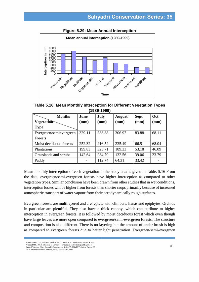
Ramachandra T.V., Subash Chandran M.D., Joshi N.V., Sreekantha, Saira V.K and
Vishnu D.M., 2013. Influence of Landscape Dynamics on Hydrological Regime in
Central Western Ghats Sahyadri Conservation Series 35, ENVIS Technical Report 65,
CES, Indian Institute of Science, Bangalore 560012, India 85
Sahyadri Conservation Series: 35
Figure 5.29: Mean Annual Interception
Table 5.16: Mean Monthly Interception for Different Vegetation Types
(1989-1999)
Months
Vegetation
Type
June
(mm)
July
(mm)
August
(mm)
Sept
(mm)
Oct
(mm)
Evergreen/semievergreen
Forests
329.11 533.38 306.97 83.88 68.11
Moist deciduous forests 252.32 416.52 235.49 66.5 68.04
Plantations 199.83 325.71 189.33 53.18 46.09
Grasslands and scrubs 142.64 234.79 132.56 39.06 23.79
Paddy - 112.74 64.31 33.42 -
Mean monthly interception of each vegetation in the study area is given in Table. 5.16 From
the data, evergreen/semi-evergreen forests have higher interception as compared to other
vegetation types. Similar conclusion have been drawn from other studies that in wet conditions,
interception losses will be higher from forests than shorter crops primarily because of increased
atmospheric transport of water vapour from their aerodynamically rough surfaces.
Evergreen forests are multilayered and are replete with climbers: lianas and epiphytes. Orchids
in particular are plentiful. They also have a thick canopy, which can attribute to higher
interception in evergreen forests. It is followed by moist deciduous forest which even though
have large leaves are more open compared to evergreen/semi-evergreen forests. The structure
and composition is also different. There is no layering but the amount of under brush is high
as compared to evergreen forests due to better light penetration. Evergreen/semi-evergreen
Mean annual interception (1989-1999)
0200400600800
10001200140016001800
Yen
neho
le
Nago
dihol
e
Hurli
hole
Ling
anam
akki
Hiliku
nji
Sha
rava
ti
Mav
inah
ole
Harid
rava
ti
Nand
ihole
Time
Inte
rcep
tio
n i
n m
m

Ramachandra T.V., Subash Chandran M.D., Joshi N.V., Sreekantha, Saira V.K and
Vishnu D.M., 2013. Influence of Landscape Dynamics on Hydrological Regime in
Central Western Ghats Sahyadri Conservation Series 35, ENVIS Technical Report 65,
CES, Indian Institute of Science, Bangalore 560012, India 86
Sahyadri Conservation Series: 35
forests are almost bare of ground vegetation and plants grow only if sufficient light penetrates
through gaps in the canopies. Plantations (acacia) show low values due to the smaller leaf size,
which reduces the overall canopy interception. Acacia and areca constitutes a major portion of
the plantation trees and have long narrow, vertically aligned leaves. Vertically aligned leaves
intercepts lesser rainfall (Valente, et al., 1997) as compared to broad leaves. Areca plantations
do have some understorey – small shrubs that yields fruit and sometimes mulching with green
leaves is practiced to prevent soil erosion during high intensity precipitation. Paddy intercepts
the least rainfall, which shows that interception is highest in trees than in crops or grasses.
Interception is highest during July as it receives the highest rainfall and lowest during
September and October as these months receive the lowest rainfall in the basin.
Figure 5.30: Mean Interception for Different Vegetation Types
Table 5.17 clearly shows the increase in interception with vegetation and rainfall. High
interception in western sub basins is due to good vegetation cover such as
evergreen/semievergreen forest and moist deciduous forests whereas the vegetation cover such
as natural forests is lesser in eastern sub basins. Plantations and agricultural activities are higher
in the eastern and southern basins.
Mean interception (1989-1999)
0
100
200
300
400
500
600
June July Aug Sept Oct
Time
Inte
rcep
tio
n i
n m
m
Evg/semievg forests
Moist deciduous
forests
Plantations
Grasslands and
scrubs
Paddy

Ramachandra T.V., Subash Chandran M.D., Joshi N.V., Sreekantha, Saira V.K and
Vishnu D.M., 2013. Influence of Landscape Dynamics on Hydrological Regime in
Central Western Ghats Sahyadri Conservation Series 35, ENVIS Technical Report 65,
CES, Indian Institute of Science, Bangalore 560012, India 87
Sahyadri Conservation Series: 35
Table 5.17: Percentage of Interception w.r.t Rainfall
Sub basins Interception (%)
Yenneholé 26.13
Nagodiholé 28.21
Hurliholé 26.73
Linganamakki 24.92
Hilkunji 27.69
Sharavathi 25.48
Mavinaholé 23.61
Haridravathi 21.82
Nandiholé 23.29
5.4 Runoff
The most common drainage pattern found in upstream river basin is dendritic. However, the
drainage density differs from west to east of the basin i.e. it decreases from west to east. Higher
densities are found in sub basins such as Yenneholé, Hurliholé, Nagodiholé and Hilkunji.
Lower drainage densities are found in Linganamakki, Sharavathi, Mavinaholé, Haridravathi
and Nandiholé. High drainage densities usually reduce the discharge in any single stream, more
evenly distributing runoff and speeding runoff into secondary and tertiary streams. Where
drainage density is very low, intense rainfall events are more likely to result in high discharge
to a few streams and therefore a greater likelihood of "flashy" discharge and flooding in humid
areas and suggests resistant bedrock.
Table 5.18 lists the drainage densities and sediment yields in the sub basins.
Table 5.18: Drainage Density and Sediment Yield
Sub basins Drainage density
(km/km2)
Sediment yield
( x 106 m3/year)
Yenneholé 2.43 0.016
Nagodiholé 2.8 0.040
Hurliholé 2.6 0.019
Linganamakki 0.9 0.354
Hilkunji 2.16 0.057
Sharavathi 1.64 0.087
Mavinaholé 1.42 0.057
Haridravathi 1.01 0.176
Nandiholé 0.74 0.11

Ramachandra T.V., Subash Chandran M.D., Joshi N.V., Sreekantha, Saira V.K and
Vishnu D.M., 2013. Influence of Landscape Dynamics on Hydrological Regime in
Central Western Ghats Sahyadri Conservation Series 35, ENVIS Technical Report 65,
CES, Indian Institute of Science, Bangalore 560012, India 88
Sahyadri Conservation Series: 35
High drainage densities and sediment yields are seen to decrease from west to east of the basin.
Western sub basins, which are highly vegetated show the highest values even though studies
show that highest values of drainage density may be found in the areas of poor vegetation cover
and its value diminishing with increasing share of surface covered with plants (Melton 1957).
The reasons for high drainage density can be due to steep slopes and clayey soil texture.
Local variability in drainage density may also be ascribed to the set of topographical and
lithological factors (Gregory and Gardiner 1975). Particularly important factors of lithology
are rock permeability and resistance to weathering and erosion. Granites and greywackes
occurring in the sub basin are of low permeability i.e. 3.1m/day to 3.4 m/day respectively.
Another factor affecting drainage density is weathering of rocks. Carlston (1963) stated that
under identical conditions of relative relief and climate, higher drainage density occurs on less
resistant lithology. Eastern sub basins such as Nandiholé and Haridravathi are characterized by
flat lands with coarse textured soil, which would have resulted in low drainage density.
Sediment yields in Table 5.18 show increase from west to east of the river basin. Though
western sub basins have steeper slopes compared to eastern sub basins e.g. Nandiholé, good
vegetation cover in the former impedes much of the sediment load and thus erosion during high
rainfall events.
Surface Runoff
Table 5.19 and 5.20 gives the mean monthly surface runoff from each sub basin and the surface
runoff generated from each land cover.
Table 5.19: Mean Monthly Surface Runoff (1989-1999)
Months
Sub basins
June
(mm)
July
(mm)
August
(mm)
September
(mm)
October
(mm)
Total
(mm)
Yenneholé 311.05 499.64 309.65 79.89 48.06 1241.96
Nagodiholé 398.42 603.27 343.27 86.37 96.16 1496.39
Hurliholé 305.97 499.79 256.57 69.39 54.67 1180.72
Linganamakki 324.11 530.22 290.1 71.36 81.74 1287.72
Hilkunji 257.06 408.14 232.17 59.98 47.94 1000.1
Sharavathi 262 364.06 176.1 48.39 76.35 914.29
Mavinaholé 218.79 356.71 176.64 52.68 80.48 871.5
Haridravathi 262 364.06 176.1 48.39 76.35 702.28
Nandiholé 141.28 217.82 139.67 42.08 95.44 623.9
Upstream 266.42 421.37 236.88 62.71 82.12 1058.05

Ramachandra T.V., Subash Chandran M.D., Joshi N.V., Sreekantha, Saira V.K and
Vishnu D.M., 2013. Influence of Landscape Dynamics on Hydrological Regime in
Central Western Ghats Sahyadri Conservation Series 35, ENVIS Technical Report 65,
CES, Indian Institute of Science, Bangalore 560012, India 89
Sahyadri Conservation Series: 35
Table 5.20: Mean Monthly Surface Runoff from Different Land covers
Months
Vegetation
Type
June
(mm)
July
(mm)
August
(mm)
Sept
(mm)
Oct
(mm)
Evergreen/semievergreen
Forests
125.02 203.38 113.65 30.03 28.35
Moist deciduous forests 125.73 205.5 115.15 30.39 24.45
Plantations 149.98 247.93 140.4 36.03 32.28
Grasslands and scrubs 189.11 315.05 175.33 47.56 99.26
Paddy 388 393.06 221.39 55.62 126.71
Open fields 475.48 795.39 448.45 119.62 126.08
Settlements 627.2 1038.43 583.81 158.37 172.16
Surface runoff progressively increases from evergreen/semievergreen forests to settlements as
seen in Figure 5.31, indicating that where there is good vegetation cover, surface runoff is less.
Forests usually have thick leaf litter and a spongy humic horizon, both of which retard surface
runoff or overland flow. Among the forest types, plantation forests showed higher runoff.
Certain species such as Tectona Grandis, which are majorly found in the eastern sub basins,
may cause severe erosion (Calder, 2002). This is due to the large leaves, which produce big
raindrops that roll of the leaves, and causes splash and subsequently rill erosion if not protected
by underbrush.
Figure5.31: Mean Monthly Surface Runoff from Different Land covers
Mean Surface Runoff (1989-1999)
0
200
400
600
800
1000
1200
June
July
Augus
t
Septe
mbe
r
Octob
er
Time
Dep
th i
n m
m
Evg/semievg
Moist deciduous
Plantations
Grasslands &
scrubsPaddy
Open fields
Settlements

Ramachandra T.V., Subash Chandran M.D., Joshi N.V., Sreekantha, Saira V.K and
Vishnu D.M., 2013. Influence of Landscape Dynamics on Hydrological Regime in
Central Western Ghats Sahyadri Conservation Series 35, ENVIS Technical Report 65,
CES, Indian Institute of Science, Bangalore 560012, India 90
Sahyadri Conservation Series: 35
Figure 5.32 shows the variation in surface runoff generation from western sub basins to eastern
sub basins portion with respect to rainfall. Table 5.21 shows the values the percentage variation
of runoff w.r.t. rainfall.
Figure 5.32: Rainfall-Surface Runoff Generation (1989-1999)
Table 5.21: Percentage of Surface Runoff w.r.t Rainfall
Sub basins Runoff (%)
Yenneholé 23.43
Nagodiholé 26.06
Hurliholé 26.77
Linganamakki 35.52
Hilkunji 24.44
Sharavathi 31.2
Mavinaholé 30
Haridravathi 36.39
Nandiholé 34.8
Low runoff generation in western (Yenneholé, Nagodiholé and Hurliholé) can be due to good
vegetation cover and lower anthropogenic activities as compared to eastern sub basins
(Mavinaholé, Haridravathi and Nandiholé). There is also high percentage of forest cover in the
western clusters, which intercepts 20-30% of the rainfall before it reaches the ground. Natural
forests are effective at retarding overland flow preventing flash floods downstream.
Agricultural activities and open fields are higher in Haridravathi and Nandiholé resulting in
higher runoff.
Rainfall-Surface Runoff (1989-1999)
01000
20003000
40005000
60007000
Yen
neho
le
Nago
dihol
e
Hurli
hole
Ling
anam
akki
Hiliku
nji
Sha
rava
ti
Mav
inah
ole
Harid
rava
ti
Nand
ihole
Depth in mm
Su
b b
asin
s

Ramachandra T.V., Subash Chandran M.D., Joshi N.V., Sreekantha, Saira V.K and
Vishnu D.M., 2013. Influence of Landscape Dynamics on Hydrological Regime in
Central Western Ghats Sahyadri Conservation Series 35, ENVIS Technical Report 65,
CES, Indian Institute of Science, Bangalore 560012, India 91
Sahyadri Conservation Series: 35
Sub Surface Runoff or Pipeflow
Table 5.22 gives the mean total sub-surface generation different sub basins. Pipes are abundant
in the Western Ghats and are a general feature in undisturbed evergreen/semievergreen forests
and moist deciduous forests. While a part of the pipe outflow is from storage build up during
previous rainfall evens, some part would presumably for current rainfall also (Putty and Prasad,
2000). Pipe outflow was not significant in the forested catchments and as observed by Putty
and Prasad, 2000, may be due to the high infiltration capacity of the soil that pipe outflow does
not create saturation of the soil.
Table 5.22: Mean Total Sub Surface Flow Generation
Sub basins Mean total pipeflow (1989-1999)
(mm)
Yenneholé 173.56
Nagodiholé 193.83
Hurliholé 142.51
Hilkunji 135.27
Sharavathi 90.57
Mavinaholé 257.07
Upstream 158.3
Here pipe flow increases from west to south of the basin. These are the areas of abundant
vegetation consisting of evergreen/semievergreen and moist deciduous forests. However,
Mavinaholé shows the highest total pipe flow as it has the lowest relief ratio. Table 5.23 shows
the percentage of pipe flow w.r.t rainfall which is a very small component.
Table 5.23 Percentage of Pipeflow w.r.t Rainfall
Sub basins Pipe flow (%)
Yenneholé 3.27
Nagodiholé 3.37
Hurliholé 3.23
Hilkunji 3.3
Sharavathi 3.03
Mavinaholé 8.85
5.5 Evapotranspiration
Table 5.24 shows the mean monthly transpiration for different vegetation types in the study
area calculated by Turc’s equation, which makes use of albedo. Albedo is observed to increase
from evergreen forests to crops with respect to openness and height of vegetation. Tall forests
Ramachandra T.V., Subash Chandran M.D., Joshi N.V., Sreekantha, Saira V.K and
Vishnu D.M., 2013. Influence of Landscape Dynamics on Hydrological Regime in
Central Western Ghats Sahyadri Conservation Series 35, ENVIS Technical Report 65,
CES, Indian Institute of Science, Bangalore 560012, India 92
Sahyadri Conservation Series: 35
with close canopy have lesser albedo than tall forests with more open canopy. Grasses and
crops are short vegetation resulting in higher albedo.
From the graph, it is observed that transpiration from evergreen/semievergreen forests is higher
compared to other vegetations. This is attributed to the albedo. Albedo from tall forests with
thick canopy is less i.e. the amount of energy reflected () is less due to internal reflections.
Lesser albedo indicates that the energy that is absorbed by the vegetation (1-) is high. It is the
absorbed energy, which is responsible for phase change i.e. from liquid water to water vapour.
Turc’s equation is radiation based and is not limited by the absence of water. Moist deciduous
forests and plantations are more open, which results in higher albedo and that means lesser
energy available for conversion of liquid water to water vapour. The mean annual transpiration
decreases from evergreen/semievergreen forests to paddy crop.
Transpiration values peak during summer when plants use up most of the water but varies with
the type of vegetation. Three factors may be playing a role in transpiration during summer i.e.
a) solar energy or insolation, b) soil moisture, c) rooting depth.
During summer, there is greater energy available for plant absorption. Absorption of this
energy by the leaf raises its temperature and its water vapour pressure. The result is that
transpiration increases along with insolation.
Transpiration is dependent on the soil moisture. The soil moisture regime in the basin is ustic
i.e it is moist for 90 or 180 days (during monsoon months) and dry during the remaining period.
However, in evergreen/semievergreen forests the soil moisture is conserved due to thick leaf
litter and since light penetration is very low, evaporation from the soil is also minimal. Thus,
during summer, soil moisture pool under an evergreen/semievergreen forests is quite high as
compared to moist deciduous or plantations, facilitating in higher transpiration.
Another factor that affects plant water uptake, in other words transpiration is the rooting depth
of plant species. Calder, 2002 indicates that studies of transpiration in dry (drought) conditions
show that the transpiration from forests is likely to be higher because of the generally increased
rooting depth of trees as compared with shorter crops such as grass and paddy and their
consequent greater access to soil water.
Evergreen, deciduous and plantation tree species mostly have taproots that are deep, but in
mature evergreen trees, shallow-rooting is usually indicated by a more swollen tree base. They
also have low root:shoot ratio i.e. the biomass in shoots are higher than roots. Buttressing
indicates a very shallow root system and are a feature of many trees in the forests of upstream
river basin. It also provides support for large trees. Since trees with buttress roots have shallow

Ramachandra T.V., Subash Chandran M.D., Joshi N.V., Sreekantha, Saira V.K and
Vishnu D.M., 2013. Influence of Landscape Dynamics on Hydrological Regime in
Central Western Ghats Sahyadri Conservation Series 35, ENVIS Technical Report 65,
CES, Indian Institute of Science, Bangalore 560012, India 93
Sahyadri Conservation Series: 35
root system, it can only survive where there is sufficient soil moisture storage in the upper soil,
especially during the lean season. But as the moisture regime in the basin is ustic, it can be
assumed that evergreen trees with non-buttressed roots may have deeper taproots to tap
moisture during summer.
Deciduous trees also have deep taproots but conserve water during summer by leaf shedding.
Leaves appear in May after a bout of convective rains in April, thus moistening the soil. Certain
plantation species such as Eucalyptus sp. is known to tap water deep from the soil creating
severe soil moisture deficit (Scott and Lesch, 1997). Such trees are known to survive in dry
areas where surface soil moisture is quite low. Grasses and crops have fibrous roots with high
root:shoot ratio i.e. the biomass of roots are higher than shoots but are shallow and therefore
cannot tap water deep from the soil. Grasses wither during dry season leaving the scrubs in the
basin. Transpiration due to crops such as paddy is the least and zero during summer as it is
grown only during rainy season. Thus, higher transpiration is observed in trees during summer
than during the monsoon and winter season.
It is also observed that transpiration is small during the monsoon period. The reason maybe
due to high vapour pressure gradient, which occurs when the vapour pressure of the air becomes
high due to high relative humidity. As a result, little transpiration occurs. Even if the rainfall
event continues over several days, transpiration cannot occur because of the high gradient.
Note: Evg/SE- evergreen/semievergreen forests; MD – moist deciduous forests
Plant- plantations; Grass- grasslands and scrubs; Agri – agricultural lands
Table 5.24: Mean Monthly Transpiration for Different Vegetation Types
Transpiration in mm
Months Evg/SE MD Plant Grass Agri Total
Jan 54.06 52.01 51.63 41.5 - 199.3
Feb 55.5 53.7 53.05 42.7 - 204.95
Mar 61 58.22 58.21 46.8 - 224.2
Apr 61.4 58.8 58.6 47.1 - 225.9
May 60.7 57.6 59.5 46.5 - 224.3
June 41.3 40.8 40.7 34 - 156.8
July 40.2 39.9 39.6 33.1 33.19 185.99
Aug 42.8 42.3 42.1 35.2 35.24 198.64
Sept 49.2 48.5 48.4 40.3 38.11 224.51
Oct 50.8 49.8 49.9 39.2 - 189.7
Nov 50.7 48.4 48.5 39.1 - 186.7
Dec 52.5 50 50.2 40.4 - 193.1

Ramachandra T.V., Subash Chandran M.D., Joshi N.V., Sreekantha, Saira V.K and
Vishnu D.M., 2013. Influence of Landscape Dynamics on Hydrological Regime in
Central Western Ghats Sahyadri Conservation Series 35, ENVIS Technical Report 65,
CES, Indian Institute of Science, Bangalore 560012, India 94
Sahyadri Conservation Series: 35
Figure 5.33: Mean Monthly Transpiration for Different Vegetation Types
The decrease in mean annual transpiration for each vegetation type is as shown in Figure 5.33.
Table 5.25 shows the mean annual transpiration of vegetation types in the basin.
Table 5.25: Mean Annual Transpiration for Different Vegetation Types
Vegetation type Mean annual transpiration
(1989-1999) (mm)
Evergreen/semievergreen forests 620.7
Moist deciduous forests 600.76
Plantations 598.32
Grasslands and scrubs 486.76
Paddy (3 months) 106.55
Table 5.26 gives the monthly evaporation for bare soil, settlements and water bodies.
Evaporation from open water is found lower compared to bare soil and settlements.
Waterbodies have very low albedo resulting in greater absorption of energy. Large and deep
water bodies such as Linganamakki reservoir also have high heat storage capacity and thermal
inertia. Solar energy penetrates to greater depth in water which results in slow heating. This
results in lesser evaporation. Since solar radiation can only penetrate a few centimeters of soil
due to its chemical composition and the structure, the air above the soil warms up much more
rapidly due to the low heat capacity of air. This results in high evaporation from soil. However,
bare soil evaporation also depends on moisture content of the soil. Wetter the soil, lower the
evaporation and vice versa. Bare soil evaporation during wet season is low as greater energy is
required to overcome the attractive forces of water and soil particles. Table 5.27 shows the
annual evaporation for each cover type.
Mean monthly transpiration (1989-1999)
0
10
20
30
40
50
60
70
Jan
Feb Mar A
pr
May Ju
nJu
lAug
Sep O
ctNov
Dec
Time
Dep
th i
n m
m
Evg
MD
Plant
Grass
Agri

Ramachandra T.V., Subash Chandran M.D., Joshi N.V., Sreekantha, Saira V.K and
Vishnu D.M., 2013. Influence of Landscape Dynamics on Hydrological Regime in
Central Western Ghats Sahyadri Conservation Series 35, ENVIS Technical Report 65,
CES, Indian Institute of Science, Bangalore 560012, India 95
Sahyadri Conservation Series: 35
Table 5.26: Mean Monthly Evaporation for Other Land covers
Months Open water
(mm)
Open fields (bare soil) (mm) /
Settlements (mm)
Total
(mm)
Jan 38.66 47.14 85.8
Feb 39.64 48.44 88.08
Mar 43.96 52.98 96.94
Apr 44.2 53.4 97.6
May 43.77 52.74 96.51
June 26.7 46.35 73.05
July 26.06 45.12 73.05
Aug 28.1 48 71.18
Sept 34.14 55.23 89.37
Oct 35.21 56.97 92.18
Nov 35.58 44.5 80.08
Dec 37.73 45.9 83.63
Figure 5.34: Mean Monthly Evaporation for Other Land covers
Table 5.27: Mean Annual Evaporation for Other Land covers
Cover type Mean annual evaporation (1989-1999)
(mm)
Open fields 596.81
Settlements 596.81
Water bodies 436.72
Mean evaporation (1989-1999)
0
10
20
30
40
50
60
Jan
Feb
Mar
Apr
May
June
July
Aug
Sept
Oct
Nov
Dec
Time
Dep
th i
n m
m Open fields &
Settlements
Water

Ramachandra T.V., Subash Chandran M.D., Joshi N.V., Sreekantha, Saira V.K and
Vishnu D.M., 2013. Influence of Landscape Dynamics on Hydrological Regime in
Central Western Ghats Sahyadri Conservation Series 35, ENVIS Technical Report 65,
CES, Indian Institute of Science, Bangalore 560012, India 96
Sahyadri Conservation Series: 35
5.6 Groundwater Recharge/Discharge
Groundwater recharge analysis results are given in Table 5.28. The rate of replenishment or
recharge is dependent on the soil moisture status, which in turn is dependent on soil texture.
Soil texture in the study area varies from loamy sand to clay loam. From soil studies, sand is
an important constituent in the basin and is responsible for high infiltration rates. Average
recharge in the basin is 30.3% of the rainfall.
Total mean monthly recharge is observed to vary from west to east with the eastern sub basins
receiving the least recharge.
Table 5.28: Mean Monthly Recharge (1989-1999)
Months
Sub basins
June
(mm)
July
(mm)
August
(mm)
September
(mm)
October
(mm)
Total
(mm)
Yenneholé 373.61 620.46 380.94 98.59 46.94 1513.76
Nagodiholé 506.22 770.94 438.34 109.72 65.5 1883.3
Hurliholé 329.02 546.28 280.09 75.23 58.44 1282.99
Linganamakki 280.83 495.75 270.88 66.03 58.7 1164.7
Hilkunji 294.71 503.31 286.14 73.55 45.44 1198.12
Sharavathi 212.25 338.87 163.59 44.53 52.81 803.28
Mavinaholé 178.7 291.96 144.72 42.68 65.12 712.04
Haridravati 125.9 217.48 135.84 42.98 63.57 576.13
Nandiholé 119.75 205.33 131.17 39.17 56.17 544.55
Upstream 220.16 360.62 200.06 55.44 59.33 886.71
Table 5.29: Mean Monthly Recharge Under Different Land use
Months
Vegetation
Type
June
(mm)
July
(mm)
August
(mm)
Sept
(mm)
Oct
(mm)
Evergreen/semievergreen
Forests
325.13 532.15 302.78 76.81 54.19
Moist deciduous forests 248.75 419.05 213.68 60.71 59.57
Plantations (areca, mango) 347.1 573.58 325.21 83.42 74.3
Grasslands and scrubs 277.98 463.39 258.34 70.06 56.56
Paddy 175.68 394.35 203.52 51.75 57.46
Open fields 201.37 337.17 190.28 50.72 53.55
Settlements 98.4 163.16 91.91 24.91 27.09

Ramachandra T.V., Subash Chandran M.D., Joshi N.V., Sreekantha, Saira V.K and
Vishnu D.M., 2013. Influence of Landscape Dynamics on Hydrological Regime in
Central Western Ghats Sahyadri Conservation Series 35, ENVIS Technical Report 65,
CES, Indian Institute of Science, Bangalore 560012, India 97
Sahyadri Conservation Series: 35
Mean monthly recharge under different land use is shown in Table 5.29. From Figure 5.35, it
is clearly observed that recharge under vegetation is higher as compared to other land cover
types. Among different vegetation types, recharge under plantation was slightly higher as
compared to natural forests (evergreen/semievergreen forests and moist deciduous forests).
Plantation trees include areca and mango. Areca plantations are a common feature in the river
basin and are extensively grown in river valleys. Lesser recharge in natural forests may be due
interception (20-30%) and diversion of infiltration water by sub surface flow (10-30%). Sub
surface flow phenomenon is not observed under plantations. Paddy, open fields and settlements
show the least recharge. It is observed from the graph that recharge peaks during July and tapers
off with decreasing rainfall.
Figure 5.35: Mean Monthly Recharge Under Different Land use
Total recharge in each sub basin was compared with total rainfall and total surface runoff to
determine any variation. Table 5.30 gives the variation in each sub basin.
Table 5.30: Rainfall-Runoff-Recharge Variation
Sub basin Rainfall (mm) Recharge (mm) Runoff (mm)
Yenneholé 5300.3 1513.76 1241.96
Nagodiholé 5740.1 1883.3 1496.39
Hurliholé 4410.1 1282.99 1180.72
Linganamakki 3623.8 1164.7 1287.72
Hilkunji 4091 1198.12 1000.1
Sharavathi 2930.3 803.28 914.29
Mavinaholé 2904.7 712.04 871.5
Haridravati 1929.6 576.13 702.28
Nandiholé 1792.7 544.55 623.9
Mean monthly recharge (1989-1999)
0
100
200
300
400
500
600
700
June
July
Aug
ust
Sep
tem
ber
Octobe
r
Time
Dep
th i
n m
m
Evg/semievg
Moist
deciduous
Plantations
(areca,
mango)Grasslands
and scrubs
Paddy
Open fields
Settlements

Ramachandra T.V., Subash Chandran M.D., Joshi N.V., Sreekantha, Saira V.K and
Vishnu D.M., 2013. Influence of Landscape Dynamics on Hydrological Regime in
Central Western Ghats Sahyadri Conservation Series 35, ENVIS Technical Report 65,
CES, Indian Institute of Science, Bangalore 560012, India 98
Sahyadri Conservation Series: 35
Figure 5.36 clearly shows the variation of recharge and runoff w.r.t rainfall. It is interesting to
note that sub basins with larger vegetation covers have higher recharge. Vegetation such as
forests not only provide shade to the ground that prevent soil water from evaporating, it
provides organic matter to the soil in the form of forest litter sand, other microorganisms etc.
Decomposition of this layer results in an organic rich top layer called humus, which enhances
infiltration rates and replenishes the aquifers. Due to higher concentration of anthropogenic
activities in the eastern basins, recharge is considerably reduced as forests are cleared for
agricultural and other purposes. Recharge is an extremely important component as it is
responsible for providing flow in rivers during dry seasons from the aquifers.
Figure 5.36: Rainfall-Runoff-Recharge (1989-1999)
Groundwater Discharge/Baseflow Analysis
The determination of groundwater volumes and flow rates requires a thorough knowledge of
the geology of the groundwater basin (Viessman, 1989). The geologic structure of a
groundwater basin governs the occurrence and movement of the groundwater beneath it. Base
flow contribution to stream flow varies widely according to the geologic nature of the aquifer.
The two major rock types occurring in the basin are gneisses /granites and greywackes.
Gneisses and granites have the lowest specific yield (3%) and occurs in the eastern portion of
the study area such as Mavinaholé, Haridravati and Nandiholé. Hence, streams here are
ephemeral indicating baseflow only during monsoon season. Western sub basins have
perennial streams, which is an indication of the rock types present in the area. The region
Rainfall-Runoff-Recharge (1989-1999)
0
1000
2000
3000
4000
5000
6000
7000
Yen
neho
le
Nago
dihol
e
Hurli
hole
Ling
anam
akki
Hiliku
nji
Sha
rava
ti
Mav
inah
ole
Harid
rava
ti
Nand
ihole
Sub basins
Dep
th i
n m
m
Rainfall
Runoff
Recharge

Ramachandra T.V., Subash Chandran M.D., Joshi N.V., Sreekantha, Saira V.K and
Vishnu D.M., 2013. Influence of Landscape Dynamics on Hydrological Regime in
Central Western Ghats Sahyadri Conservation Series 35, ENVIS Technical Report 65,
CES, Indian Institute of Science, Bangalore 560012, India 99
Sahyadri Conservation Series: 35
consists of greywackes, which has higher specific yield of 27%. Discharge for each sub basin
is given in Table 5.31.
Table 5.31: Mean Total Discharge (1989-1999)
Sub basins Mean total discharge
(1989-1999) (mm)
Yenneholé 225.98
Nagodiholé 463.95
Hurliholé 192.44
Linganamakki 174.7
Hilkunji 179.71
Sharavathi 120.49
Mavinaholé 21.36
Haridravati 17.28
Nandiholé 16.33
Upstream 92.05
Another important reason for better discharge in western sub basins is the good vegetation
cover. Natural forests retard much of the overland flow facilitating in enhanced infiltration and
thus recharge. In other words, regardless of the geology the amount of water entering an aquifer
is dependent first on the vegetation and soil present in the area. Forestlands cleared for
agriculture or other purposes increases overland flow thus decreasing recharge and subsequent
discharge into the streams.
Well Behavioral Analysis
Water table levels of ten wells were available to observe groundwater fluctuations and behavior
in the basin. These wells were mainly located in eastern portion and southern portion of the
study area. Well data for western sub basins were not available. Table 5.32 gives the long term
trend and amplitude in each well.

Ramachandra T.V., Subash Chandran M.D., Joshi N.V., Sreekantha, Saira V.K and
Vishnu D.M., 2013. Influence of Landscape Dynamics on Hydrological Regime in
Central Western Ghats Sahyadri Conservation Series 35, ENVIS Technical Report 65,
CES, Indian Institute of Science, Bangalore 560012, India 100
Sahyadri Conservation Series: 35
Table 5.32: Long Term Trend and Amplitude in Selected Wells in Upstream
Well Nos. Amplitude Depth to Water
Table
170504 Strong dampening Increasing
170511 Slight dampening Increasing
170510 Strong dampening Increasing
170502 Strong dampening Increasing
170410 Strong dampening Decreasing
170402 Strong dampening Decreasing
170406 Slight dampening Increasing
170401 Strong dampening Increasing
170404 Strong dampening Decreasing
170903 Strong dampening Increasing
It is interesting to note that wells showing increase in water depth had dampening effect with
some showing strong effects. Dampening indicates reduction in amplitude, which may be due
to groundwater overexploitation occurring during the rainy season (June-August) with the
result that well levels are unable to rise even during heavy rainfall. Other reasons may include
groundwater irrigation and the type of irrigation practiced or the downstream overexploitation
of ground water, which has affected well levels upstream. The dampening effect is seen
beginning from 1994-1999 in all wells.
Well no. 170404 showed decrease in the depth to water table with strong dampening. The
reason may be due to the fact that water logging by damming Linganamakki reservoir would
have increased recharge or downstream pumping may have changed the geometry of the basin.
Also, as it is along the ridgeline there is quicker drainage of water, which would have increased
the water levels. Well nos 170410 and 170402 are located in Haridravati and Nandiholé sub
basin respectively. Both these wells showed decrease in depth to water table i.e. the water table
must be rising in these regions but shows strong dampening effect due to over extraction of
groundwater.
Figure 5.37 depict the water table depths in well. Negative values actually indicate the water
levels below ground. Zero is considered the ground level or reference level.

Ramachandra T.V., Subash Chandran M.D., Joshi N.V., Sreekantha, Saira V.K and
Vishnu D.M., 2013. Influence of Landscape Dynamics on Hydrological Regime in
Central Western Ghats Sahyadri Conservation Series 35, ENVIS Technical Report 65,
CES, Indian Institute of Science, Bangalore 560012, India 101
Sahyadri Conservation Series: 35
Figure 5.37 Water Table Depths (bgl) in Selected Wells Upstream (1989-1999)
Well level 1989-1999
170504
-20
-15
-10
-5
0
Ja
n-8
9
Ju
l-8
9
Ja
n-9
0
Ju
l-9
0
Ja
n-9
1
Ju
l-9
1
Ja
n-9
2
Ju
l-9
2
Ja
n-9
3
Ju
l-9
3
Ja
n-9
4
Ju
l-9
4
Ja
n-9
5
Ju
l-9
5
Ja
n-9
6
Ju
l-9
6
Ja
n-9
7
Ju
l-9
7
Ja
n-9
8
Ju
l-9
8
Ja
n-9
9
Ju
l-9
9
Time
bg
l in
me
ters
Well levels 1989-1999 170511
-12
-10
-8
-6
-4
-2
0
Ja
n-8
9
Ju
l-8
9
Ja
n-9
0
Ju
l-9
0
Ja
n-9
1
Ju
l-9
1
Ja
n-9
2
Ju
l-9
2
Ja
n-9
3
Ju
l-9
3
Ja
n-9
4
Ju
l-9
4
Ja
n-9
5
Ju
l-9
5
Ja
n-9
6
Ju
l-9
6
Ja
n-9
7
Ju
l-9
7
Ja
n-9
8
Ju
l-9
8
Ja
n-9
9
Ju
l-9
9
Time
bg
l in
me
ters
Well levels 1989-1999
170510
-20
-15
-10
-5
0
Jan
-89
Jul-
89
Jan
-90
Jul-
90
Jan
-91
Jul-
91
Jan
-92
Jul-
92
Jan
-93
Jul-
93
Jan
-94
Jul-
94
Jan
-95
Jul-
95
Jan
-96
Jul-
96
Jan
-97
Jul-
97
Jan
-98
Jul-
98
Jan
-99
Jul-
99
Time
bg
l in
me
ters

Ramachandra T.V., Subash Chandran M.D., Joshi N.V., Sreekantha, Saira V.K and
Vishnu D.M., 2013. Influence of Landscape Dynamics on Hydrological Regime in
Central Western Ghats Sahyadri Conservation Series 35, ENVIS Technical Report 65,
CES, Indian Institute of Science, Bangalore 560012, India 102
Sahyadri Conservation Series: 35
Well levels 1989-1999
170502
-20
-15
-10
-5
0
Jan-8
9
Jul-89
Jan-9
0
Jul-90
Jan-9
1
Jul-91
Jan-9
2
Jul-92
Jan-9
3
Jul-93
Jan-9
4
Jul-94
Jan-9
5
Jul-95
Jan-9
6
Jul-96
Jan-9
7
Jul-97
Jan-9
8
Jul-98
Jan-9
9
Jul-99
Time
Well
levels
Well levels 1989-1999
170410
-16-14-12-10
-8-6-4-20
Ja
n-8
9
Ju
l-8
9
Ja
n-9
0
Ju
l-9
0
Ja
n-9
1
Ju
l-9
1
Ja
n-9
2
Ju
l-9
2
Ja
n-9
3
Ju
l-9
3
Ja
n-9
4
Ju
l-9
4
Ja
n-9
5
Ju
l-9
5
Ja
n-9
6
Ju
l-9
6
Ja
n-9
7
Ju
l-9
7
Ja
n-9
8
Ju
l-9
8
Ja
n-9
9
Ju
l-9
9Time
bg
l in
me
ters
Well levels 1989-1999
170402
-10.00
-8.00
-6.00
-4.00
-2.00
0.00
Jan-8
9
Jul-89
Jan-9
0
Jul-90
Jan-9
1
Jul-91
Jan-9
2
Jul-92
Jan-9
3
Jul-93
Jan-9
4
Jul-94
Jan-9
5
Jul-95
Jan-9
6
Jul-96
Jan-9
7
Jul-97
Jan-9
8
Jul-98
Jan-9
9
Jul-99
Time
Well levels

Ramachandra T.V., Subash Chandran M.D., Joshi N.V., Sreekantha, Saira V.K and
Vishnu D.M., 2013. Influence of Landscape Dynamics on Hydrological Regime in
Central Western Ghats Sahyadri Conservation Series 35, ENVIS Technical Report 65,
CES, Indian Institute of Science, Bangalore 560012, India 103
Sahyadri Conservation Series: 35
Well levels 1989-1999
170406
-14-12-10
-8-6-4-20
Ja
n-8
9
Ju
l-8
9
Ja
n-9
0
Ju
l-9
0
Ja
n-9
1
Ju
l-9
1
Ja
n-9
2
Ju
l-9
2
Ja
n-9
3
Ju
l-9
3
Ja
n-9
4
Ju
l-9
4
Ja
n-9
5
Ju
l-9
5
Ja
n-9
6
Ju
l-9
6
Ja
n-9
7
Ju
l-9
7
Ja
n-9
8
Ju
l-9
8
Ja
n-9
9
Ju
l-9
9
Time
bg
l in
mete
rs
Well levels 1989-1999
170401
-14-12-10-8-6-4-20
Jan-8
9
Jul-89
Jan-9
0
Jul-90
Jan-9
1
Jul-91
Jan-9
2
Jul-92
Jan-9
3
Jul-93
Jan-9
4
Jul-94
Jan-9
5
Jul-95
Jan-9
6
Jul-96
Jan-9
7
Jul-97
Jan-9
8
Jul-98
Jan-9
9
Jul-99
Time
bg
l in
mete
rs
Well levels 1989-1999
170404
-14-12-10
-8-6-4-20
Ja
n-8
9
Ju
l-8
9
Ja
n-9
0
Ju
l-9
0
Ja
n-9
1
Ju
l-9
1
Ja
n-9
2
Ju
l-9
2
Ja
n-9
3
Ju
l-9
3
Ja
n-9
4
Ju
l-9
4
Ja
n-9
5
Ju
l-9
5
Ja
n-9
6
Ju
l-9
6
Ja
n-9
7
Ju
l-9
7
Ja
n-9
8
Ju
l-9
8
Ja
n-9
9
Ju
l-9
9
Time
bg
l in
me
ters
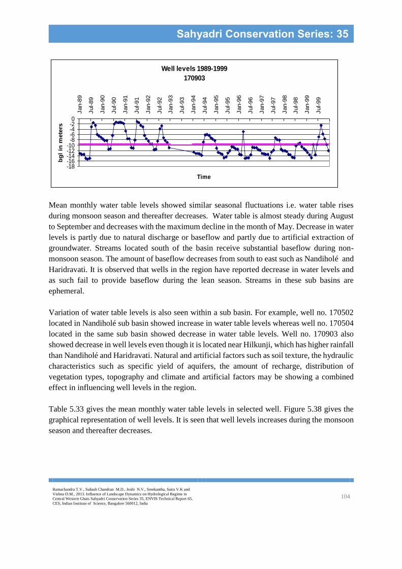
Ramachandra T.V., Subash Chandran M.D., Joshi N.V., Sreekantha, Saira V.K and
Vishnu D.M., 2013. Influence of Landscape Dynamics on Hydrological Regime in
Central Western Ghats Sahyadri Conservation Series 35, ENVIS Technical Report 65,
CES, Indian Institute of Science, Bangalore 560012, India 104
Sahyadri Conservation Series: 35
Mean monthly water table levels showed similar seasonal fluctuations i.e. water table rises
during monsoon season and thereafter decreases. Water table is almost steady during August
to September and decreases with the maximum decline in the month of May. Decrease in water
levels is partly due to natural discharge or baseflow and partly due to artificial extraction of
groundwater. Streams located south of the basin receive substantial baseflow during non-
monsoon season. The amount of baseflow decreases from south to east such as Nandiholé and
Haridravati. It is observed that wells in the region have reported decrease in water levels and
as such fail to provide baseflow during the lean season. Streams in these sub basins are
ephemeral.
Variation of water table levels is also seen within a sub basin. For example, well no. 170502
located in Nandiholé sub basin showed increase in water table levels whereas well no. 170504
located in the same sub basin showed decrease in water table levels. Well no. 170903 also
showed decrease in well levels even though it is located near Hilkunji, which has higher rainfall
than Nandiholé and Haridravati. Natural and artificial factors such as soil texture, the hydraulic
characteristics such as specific yield of aquifers, the amount of recharge, distribution of
vegetation types, topography and climate and artificial factors may be showing a combined
effect in influencing well levels in the region.
Table 5.33 gives the mean monthly water table levels in selected well. Figure 5.38 gives the
graphical representation of well levels. It is seen that well levels increases during the monsoon
season and thereafter decreases.
Well levels 1989-1999
170903
-18-16-14-12-10-8-6-4-20
Jan-8
9
Jul-89
Jan-9
0
Jul-90
Jan-9
1
Jul-91
Jan-9
2
Jul-92
Jan-9
3
Jul-93
Jan-9
4
Jul-94
Jan-9
5
Jul-95
Jan-9
6
Jul-96
Jan-9
7
Jul-97
Jan-9
8
Jul-98
Jan-9
9
Jul-99
Time
bg
l in
mete
rs

Ramachandra T.V., Subash Chandran M.D., Joshi N.V., Sreekantha, Saira V.K and
Vishnu D.M., 2013. Influence of Landscape Dynamics on Hydrological Regime in
Central Western Ghats Sahyadri Conservation Series 35, ENVIS Technical Report 65,
CES, Indian Institute of Science, Bangalore 560012, India 105
Sahyadri Conservation Series: 35
Table 5.33: Mean Monthly Water Table Levels in Selected Wells (1989-1999)
170504 170511 170510 170502 170410 170402 170406 170401 170404 170903
Jan 11.71 7.33 8.63 1.6 8.94 4.33 8.55 8.35 5.33 10.95
Feb 11.96 7.76 8.94 1.78 9.49 4.96 8.53 9.23 6.2 11.75
Mar 12.03 8.05 9.03 1.88 9.72 5.12 9.58 9.35 6.73 11.15
Apr 13.14 9.14 10.88 2.22 11.31 5.93 11.29 10.64 8.45 12.79
May 13.46 9.25 10.89 2.31 11.8 6.17 11.76 10.74 8.73 13.57
June 11.06 7.21 7.3 0.87 10.42 3.8 9.96 8.82 6.1 11.29
Jul 8.16 4.82 5.19 0.6 5.95 1.47 5.29 4.58 1.55 7.16
Aug 8.1 4.3 4.73 0.57 4.32 1.36 4.08 4.18 1.36 5.5
Sept 8.16 4.62 5.02 0.56 4.75 1.99 5.19 5.24 2.13 6.43
Oct 9.08 5.17 5.87 0.89 6.14 2.71 6.69 6.7 2.89 7.35
Nov 10.29 6.2 7.14 1.14 6.87 3.27 7.2 7.25 3.32 8.66
Dec 10.66 6.56 7.73 1.37 7.49 3.79 7.73 7.93 4.43 9.47
Figure 5.38: Mean Monthly Water Table Levels in Selected Wells (1989-1999)
5.7 Water Budget
Water budgeting was done sub-basinwise in the river basin. For example, water budget for
Yenneholé was estimated for each month in Table 5.34. Change in storage in Yenneholé sub
basin is given in Figure 5.39.
Water Table Levels in Selected Wells (1989-1999)
0
2
4
6
8
10
12
14
16
Jan
Feb
Mar
Apr
May
Jun
Jul
Aug
Sep
Oct
Nov
Dec
Time
Dep
th t
o W
ate
r T
ab
le i
n
mete
rs
170504
170511
170510
170502
170410
170402
170406
170401
170404
170903
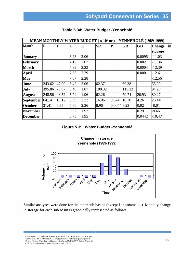
Ramachandra T.V., Subash Chandran M.D., Joshi N.V., Sreekantha, Saira V.K and
Vishnu D.M., 2013. Influence of Landscape Dynamics on Hydrological Regime in
Central Western Ghats Sahyadri Conservation Series 35, ENVIS Technical Report 65,
CES, Indian Institute of Science, Bangalore 560012, India 106
Sahyadri Conservation Series: 35
Table 5.34: Water Budget -Yenneholé
MEAN MONTHLY WATER BUDGET ( x 106 m3) – YENNEHOLÉ (1989-1999)
Month R I T E SR P GR GD Change in
storage
January 6.93 2.06 0.0095 -11.03
February 7.12 2.07 0.002 -11.36
March 7.82 2.23 0.0004 -12.39
April 7.88 2.29 0.0001 -12.6
May 7.87 2.28 -12.56
June 243.62 47.09 5.42 2.06 62.37 69.38 55.09
July 395.86 76.87 5.40 1.87 100.32 115.12 94.28
August 248.56 48.52 5.74 1.96 62.26 70.74 20.93 80.27
September 64.14 13.12 6.59 2.22 16.06 0.674 18.30 4.26 26.44
October 31.41 6.35 6.60 2.36 8.96 0.0044 8.23 0.92 -0.01
November 6.52 1.97 0.29 -9.65
December 6.75 1.95 0.0442 -10.47
Figure 5.39: Water Budget -Yenneholé
Similar analyses were done for the other sub basins (except Linganamakki). Monthly change
in storage for each sub basin is graphically represented as follows.
Change in storage
Yennehole (1989-1999)
-20
0
20
40
60
80
100
Janu
ary
Febru
ary
Mar
chApr
il
May
June
July
Aug
ust
Sep
tem
ber
Octobe
r
Nove
mbe
r
Dece
mbe
r
Time
Vo
lum
e i
n m
illi
on
cu
.m

Ramachandra T.V., Subash Chandran M.D., Joshi N.V., Sreekantha, Saira V.K and
Vishnu D.M., 2013. Influence of Landscape Dynamics on Hydrological Regime in
Central Western Ghats Sahyadri Conservation Series 35, ENVIS Technical Report 65,
CES, Indian Institute of Science, Bangalore 560012, India 107
Sahyadri Conservation Series: 35
Figure 5.40: Water Budget -Nagodiholé
Figure 5.41: Water Budget -Hurliholé
Change in storage
Nagodihole (1989-1999)
-20
0
20
40
60
80
Janu
ary
Febru
ary
Mar
chApr
il
May
June
July
Aug
ust
Sep
tem
ber
Octobe
r
Nove
mbe
r
Dece
mbe
r
Time
Vo
lum
e i
n m
illi
on
cu
.m
Change in storage
Hurlihole (1989-1999)
-100
10
203040
Janu
ary
Feb
ruar
yM
arch
Apr
il
May
June
July
Aug
ust
Sep
tem
ber
Oct
obe
rNove
mbe
rDece
mbe
r
Time
Vo
lum
e i
n m
illi
on
cu
.m

Ramachandra T.V., Subash Chandran M.D., Joshi N.V., Sreekantha, Saira V.K and
Vishnu D.M., 2013. Influence of Landscape Dynamics on Hydrological Regime in
Central Western Ghats Sahyadri Conservation Series 35, ENVIS Technical Report 65,
CES, Indian Institute of Science, Bangalore 560012, India 108
Sahyadri Conservation Series: 35
Figure 5.42 Water Budget - Hilkunji
Figure 5.43: Water Budget - Sharavathi
Figure 5.44: Water Budget - Mavinaholé
Change in storage
Hilkunji (1989-1999)
-10
010
2030
40
Janu
ary
Febru
ary
Mar
chApr
il
May
June
July
Aug
ust
Sep
tem
ber
Octobe
r
Nove
mbe
r
Dece
mbe
r
Time
Vo
lum
e i
n m
illi
on
cu
.m
Change in storage
Sharavati (1989-1999)
-10
010
2030
40
Janu
ary
Febru
ary
Mar
chApr
il
May
June
July
Aug
ust
Sep
tem
ber
Octobe
r
Nove
mbe
r
Dece
mbe
r
Time
Vo
lum
e i
n m
illi
on
cu
.m
Change in storage
Mavinahole (1989-1999)
-10-505
1015202530
Janu
ary
Febru
ary
Mar
chApr
il
May
June
July
Aug
ust
Sep
tem
ber
Octobe
r
Nove
mbe
r
Dece
mbe
r
Time
Vo
lum
e i
n m
illi
on
cu
.m

Ramachandra T.V., Subash Chandran M.D., Joshi N.V., Sreekantha, Saira V.K and
Vishnu D.M., 2013. Influence of Landscape Dynamics on Hydrological Regime in
Central Western Ghats Sahyadri Conservation Series 35, ENVIS Technical Report 65,
CES, Indian Institute of Science, Bangalore 560012, India 109
Sahyadri Conservation Series: 35
Figure 5.45: Water Budget - Haridravathi
Figure 5.46: Water Budget - Nandiholé
Change in storage
Haridravati (1989-1999)
-20
-10
0
10
20
30
Janu
ary
Febru
ary
Mar
chApr
il
May
June
July
Aug
ust
Sep
tem
ber
Octobe
r
Nove
mbe
r
Dece
mbe
r
Time
Vo
lum
e i
n c
u.m
Change in storage
Nandihole (1989-1999)
-10
-5
0
5
10
15
Janu
ary
Febru
ary
Mar
chApr
il
May
June
July
Aug
ust
Sep
tem
ber
Octobe
r
Nove
mbe
r
Dece
mbe
r
Time
Vo
lum
e i
n c
u.m

Ramachandra T.V., Subash Chandran M.D., Joshi N.V., Sreekantha, Saira V.K and
Vishnu D.M., 2013. Influence of Landscape Dynamics on Hydrological Regime in
Central Western Ghats Sahyadri Conservation Series 35, ENVIS Technical Report 65,
CES, Indian Institute of Science, Bangalore 560012, India 110
Sahyadri Conservation Series: 35
Figure 5.47: Water Budget – Upstream
The total change in storage for each sub basin is given in Table 5.35. Storage consists of the
water contained in soil and the underlying rock. Higher storage in western sub basins are
responsible for the lush vegetation present in these areas. During summer, the plants can extract
sufficient moisture from the soil for its physiological processes.
Table 5.35: Total Storage in Sub Basins
Sub basins Mean Total Storage (x 106 M cu.m)
(June-Oct)
Yenneholé 233.09
Nagodiholé 171.56
Hurliholé 86.80
Linganamakki 834.69
Hilkunji 68.55
Sharavathi 70.54
Mavinaholé 48.03
Haridravathi 51.21
Nandiholé 17.6
Mean annual volumes of hydrological components in each sub basin are given in Table 5.36.
Change in storage
Upstream (1989-1999)
-200
0
200
400
600
800
Jan Feb Mar Apr May Jun Jul Aug Sep Oct Nov Dec
Time
Vo
lum
e i
n m
illi
on
cu
.m

Ramachandra T.V., Subash Chandran M.D., Joshi N.V., Sreekantha, Saira V.K and
Vishnu D.M., 2013. Influence of Landscape Dynamics on Hydrological Regime in
Central Western Ghats Sahyadri Conservation Series 35, ENVIS Technical Report 65,
CES, Indian Institute of Science, Bangalore 560012, India 111
Sahyadri Conservation Series: 35
Table 5.36: Mean Annual Volumes of Hydrological Component ( x 106 m3) (1989-1999)
Sub basins R I T E SR P GR GD
Yenneholé 983.6 191.96 80.7 25.37 281.78 0.67 286.79 26.47
Nagodiholé 374.68 86.63 32.22 6.7 88.91 0.79 115.75 16.98
Hurliholé 413.69 85.32 42.13 12.74 111.88 0.62 200.72 11.55
Linganamakki 2915.53 379.06 265.12 228.73 815.2 - 749.01 78.05
Hilkunji 337.85 77.31 39.45 7.72 83.03 0.8 99.38 9.23
Sharavathi 358.68 61.53 50.4 17.89 119.0 0.26 105.46 9.46
Mavinaholé 254.41 42.71 33.16 13.58 78.81 0.3 64.97 1.17
Haridravathi 555.82 77.56 90.3 51.25 188.13 - 184.79 3.25
Nandiholé 31.08 49.84 61.24 29.67 125.3 - 97.37 1.86
Table 5.37: Mean Monthly Stream flow Contribution in Sub Basins
(x 106 m3) (1989-1999)
Sub
basin
Yenne Nagod Hurli Lingan Hili Shara Mavin Hari Nandi
Jan 0.0095 0.029 0.008 0.039 0.002 0.002 0.002 0.002 0.002
Feb 0.0021 0.006 0.001 0.008 0.0006 0.0005 0.0004 0.0003 0.0002
Mar 0.0004 0.001 0.0004 0.001 0.00018 0.00016 0.00015 0.0001 0.0001
Apr 0.0001 0.0002 0.0002 0.0004 - - - - -
May - 0.0001 - 0.0002 - - - - -
Jun 69.38 35.34 28.87 204.14 21.25 33.85 19.63 35.47 28.87
Jul 115.11 20.11 47.16 333.96 33.74 47.07 32.01 70.35 47.16
Aug 91.67 19.84 33.36 237.84 27.24 30.3 15.85 44.01 33.63
Sept 23.25 19.29 9.03 62.97 6.44 7.79 5.96 16.63 9.03
Oct 9.16 2.75 5.49 53.21 4.29 9.62 6.77 24.77 5.49
Nov 0.29 0.59 0.09 0.87 0.09 0.065 0.04 0.12 0.09
Dec 0.044 0.13 0.01 0.19 0.01 0.01 0.009 0.019 0.01
The mean monthly stream flow contribution for all sub basins is given in Table 5.37. It is the
sum of surface runoff, sub surface runoff (pipeflow) and groundwater discharge. Natural and
artificial forces operating over a watershed or a basin ultimately impacts its stream flow regime.
Perenniality of streams is dependent on factors such as geology, type and distribution of
vegetation, soil, climate and topography. Western clusters enjoys the benefit of good rainfall,
vegetation and geology to give rise to stream flow even during the lean season. A contrast is
seen on the eastern side as volume of stream progressively decreases from Hilkunji to
Nandiholé sub basins. Modification of land by agriculture and other uses, unfavourable
geology, clearcutting of natural forests and poor rainfall have resulted in decline in baseflow
during the non-monsoon months and significant decrease during summer (Mar-May).

Ramachandra T.V., Subash Chandran M.D., Joshi N.V., Sreekantha, Saira V.K and
Vishnu D.M., 2013. Influence of Landscape Dynamics on Hydrological Regime in
Central Western Ghats Sahyadri Conservation Series 35, ENVIS Technical Report 65,
CES, Indian Institute of Science, Bangalore 560012, India 112
Sahyadri Conservation Series: 35
The evergreen forests have high humidity thereby are the major driving forces in determining
the amount of rainfall in these regions. Thus in the upstream, heavy rainfall occurs along
Nagodi, Kogar and Aralagodu raingauge stations. Forest cover in these regions is also high
(land cover analysis, land use analysis) indicating the close relationships between rainfall in
Western Ghats regions with the type (evergreen, semi-evergreen) and spatial extent of
vegetation cover (Table 5.38). Within the catchment area of Linganamakki, the areas
surrounded by rich vegetation like Nagara, Karimane, Byakodu receive high rainfall compared
to fragmented, poorly vegetated eastern regions like Ulluru, Anandapura and Ripponpet.
It is found that western side sub-basins (Nagodihole, Hurulihole, Yennehole) have rain fall
ranges from 4500-6500 mm and their stream flow is quite high having grade of A (perennial
streams). Sub-basinwise stream flow is given in Table 5.39. South east region (Sharavathi,
Hilkunji) has rain fall of around 5000mm with stream flow moderate to high having grading of
B-C (stream flow for 6-9 months). Finally sub-basins of eastern side (Nandihole, Haridravathi
and Mavinahole) have rain fall of 1400-3000 mm which is very less and their stream flow is
also quite low, graded C-D (4-6 months: mostly during monsoon). Table 5.38: Land-use pattern (%) and associated annual rainfall in the sub-basins of Sharavathi river upstream
Locality Annual rainfall (mm) Forests EVG/SE MD Plantation Grassland Agri Open Sett
Nandihole 1715.20 1.25 27.34 2.93 29.73 10.55 23.14 5.05
Haridravathi 1776.49 1.3 21.77 3.91 26.82 16.76 24.63 4.81
Mavinahole 2157.88 2.44 35.09 5.04 21.19 10.66 18.72 6.85
Sharavathi 3382.40 11.54 28.80 10.03 11.58 13.72 19.34 5.00
Hilkunji 4801.25 29.84 34.74 6.45 7.56 5.72 11.46 4.25
Hurulihole 4410.05 22.94 31.54 8.28 13.85 1.28 18.92 3.19
Nagodi 5597.50 40.51 23.54 13.73 4.78 0.05 13.03 4.35
Yennehole 4933.01 27.32 22.94 14.75 11.50 1.04 19.40 3.05
Linganamakki 3423.25 8.51 34.14 9.35 2.26 8.51 32.88 4.34
* Water body constitutes 15.8% of the region, Note: EVG/SE: Evergreen/semi evergreen; MD: Moist deciduous; Agri: Agriculture; open:
open area; sett: settlements
Table 5.39: Stream flow data for major tributaries of streams in the Linganamakki catchment
Stream flow measurement (Discharge m3/sec) ------------------------------------------------------------------------------
Stream Location Oct. Nov. Dec. Jan Stream
Grading*
Nandihole Northeast 1.23 3.68 0.09 0.000 D
Haridravathi East 16.23 3.02 0.46 0.000 D
Mavinahole East 5.93 3.00 0.44 0.000 D
Sharavathi Southeast 26.73 5.83 1.08 0.964 C
Hilkunji Southeast 46.27 10.64 2.64 1.670 B
Nagodihole West 22.56 4.84 1.90 1.420 A
Hurlihole West 6.30 1.37 0.78 0.661 A
Yennehole West NM 13.40 1.81 1.680 A
* Based on numbers of months with flow a: 12 months, B: 9 months; C: 6 months and D: 4 months

Ramachandra T.V., Subash Chandran M.D., Joshi N.V., Sreekantha, Saira
V.K and Vishnu D.M., 2013. Influence of Landscape Dynamics on
Hydrological Regime in Central Western Ghats Sahyadri Conservation Series
35, ENVIS Technical Report 65, CES, Indian Institute of Science, Bangalore
560012, India
113
SAHYADRI CONSERVATION SERIES 35, ETR 65 - 2013
6.0 Conclusions
This study explored and quantified the altered hydrological parameters due to large scale land
use and land cover changes. In this regard, satellite data has offered excellent inputs to monitor
dynamic changes through repetitive, synoptic and accurate information of the changes in a river
basin. It also provided a means of observing hydrological state variables over large areas, which
was useful in parameter estimation of hydrologic models. GIS offered means for merging
various spatial themes (data layers) that was useful in interpretation, analysis and change
detection of spatial structures and objects. Studies reveal the linkages among variables such as
land use, hydrology and ecology. Following are the conclusions drawn from the hydrological
studies of upstream, river basin.
Rainfall analysis based on one hundred years data for Sagara and Hosanagara show reduction
of –3.55% and 5% respectively in the Sharavathi upstream river basin Regression analysis was
carried out for each rain gauge station considering rainfall as dependent variable and latitude,
longitude, altitude and land cover as independent variables. Regression analysis showed
rainfall having significant relationship (5% level of significance) between land cover, latitude,
longitude, and altitude.
Interception was comparatively high in evergreen/semievergreen forests due to thicker and
multilayered canopies. It was followed by moist deciduous forests, plantations, scrub savanna
and paddy. Interception was the highest during peak rainfall months and showed least values
for shorter crops.
Transpiration also decreased from evergreen/semi-evergreen forests to paddy due to lower
albedo in the former. Lower albedo corresponds to higher latent energy, which converts liquid
water to water vapour. Transpiration peaks during summer and is the lowest during the
monsoon season. Low transpiration during wet months is because most of the energy available
for evaporation is consumed by the interception process, which precedes transpiration and
because solar radiation is inhibited by clouds in the wet months (Shuttleworth, 1993).
Catchments with good forest (evergreen/semi-evergreen and moist deciduous forests) cover
showed reduced runoff as compared to catchments with poor forest covers. The results are
similar to conclusions drawn by Bosch and Hewlett, 1982 from various catchment experiments
that forested areas have reduced runoff as compared with those under shorter vegetation.
Runoff and thus erosion from plantation forests was higher from that of natural forests. Erosion
rates in undisturbed natural forest could be considered to represent a natural baseline or
background erosion rates against which the erosion rates from all other land uses.

Ramachandra T.V., Subash Chandran M.D., Joshi N.V., Sreekantha, Saira
V.K and Vishnu D.M., 2013. Influence of Landscape Dynamics on
Hydrological Regime in Central Western Ghats Sahyadri Conservation Series
35, ENVIS Technical Report 65, CES, Indian Institute of Science, Bangalore
560012, India
114
SAHYADRI CONSERVATION SERIES 35, ETR 65 - 2013
Sub-surface flow caused by pipes in the Western Ghats appears at valley bottoms of forested
slopes. The macropore flow collects in the pipes and flows through them into the stream.
Recharge in the sub basins varied with respect to vegetal cover and soil texture. Higher recharge
was observed in sub basins with good forest cover.
Sub basins with good forest cover showed good amount of dry season flow for all 12 months
with the flow decreasing as we move towards east. Decrease of low flows in eastern sub basins
can be partly attributed to eucalyptus plantations. Eucalyptus trees have deep roots that tap
water deep in the soil mantle creating severe soil moisture deficits. It may take many years of
rainfall before field capacity conditions can be established and recharge of the groundwater
aquifer and perennial flows can take place. Another reason is the low specific yield of the
underlying rock.
This highlights the impacts of tropical forests on dry season flows as the infiltration properties
of the forest are critical on the available water partitioned between runoff and recharge (leading
to increased dry season flows).
In short, sub basins with good vegetation cover i.e. natural forests and low anthropogenic
activities especially in the western sub basins had high interception, transpiration, recharge and
discharge and low surface runoff. On the other hand, eastern sub basins with less natural forest
cover had low interception, transpiration, recharge and discharge and high surface runoff.
The anthropogenic influences on the land cover are related to the land use for agriculture,
plantation forestry and urbanisation. It was obvious from the present study that land use has an
implication on the hydrological components operating in the river basin. However, further
research may be necessary to understand the scale of study, low flow mechanism in rivers, sub
surface flow distribution under forests in Western Ghats etc.
Some studies that need to be considered in the future analysis are discussed below.
a) The scale of study is important as macro level understanding of the hydrology of a river
basin may not be enough to capture the dynamics as some changes are relevant only at
micro scale. For example, clearing a few hectares of forest may not influence the regional
or global hydrological cycle but it can have implications on the local water cycle. Impact
on the local water cycle can affect the micro ecosystem, which may harbour flora and fauna
that are adapted to that type of an environment. A water balance study should thus link the
ecology and hydrology of a river basin so as to understand the complexities of a region.
Ecohydrology describes species diversity, growth forms of vegetation, biomass estimates
etc and fuses it with hydrology. Another important area of study is the geology, which is
helpful in understanding the occurrence and distribution of ground water and thus the low
Ramachandra T.V., Subash Chandran M.D., Joshi N.V., Sreekantha, Saira
V.K and Vishnu D.M., 2013. Influence of Landscape Dynamics on
Hydrological Regime in Central Western Ghats Sahyadri Conservation Series
35, ENVIS Technical Report 65, CES, Indian Institute of Science, Bangalore
560012, India
115
SAHYADRI CONSERVATION SERIES 35, ETR 65 - 2013
flow regime of a river. It is important to have a holistic approach when dealing with river
basins rather than a pure engineering or ecological approach.
b) Interception analysis in the present study takes into account only the storage capacity and
its associated evaporative fraction, intensity of rainfall and seasonality of vegetation.
Interception is also dependent on leaf thickness, leaf and stem roughness and leaf
orientation, which varies with species. Components such as stemflow and throughfall have
not been considered and have to be included in future analysis.
c) Field studies of soil are required to determine the soil infiltration rates. In the present study,
infiltration is the difference of net rainfall and surface runoff and the actual values may
differ. Studies have proved that infiltration under forested areas in Western Ghats is high.
d) Sub surface flow distribution through pipes in Western Ghats has only been studied in the
past few years. Pipeflow have been observed to contribute to flow in streams and in Western
Ghats, many dug wells are known to derive their water from large diameter pipes. In regions
where Hortonian flow cannot occur, it is observed that pipe overland flow which is new
mechanism of runoff generation occurs. This has not been quantified in the studies and
needs to be included in future analysis. Studies are also needed to understand the extent
and distribution of pipes under forested slopes.
e) Low flow contribution to stream flow in the study area takes into consideration only the
natural factors and not artificial factors such as pumping. The effects of groundwater
pumping near the head of a perennial river may result in groundwater table depletion
through tapping of recharge water. This can result in substantial environmental degradation
of the river habitats, loss of naturally sustained fisheries, reduction in the general amenity
value of the river. Monitoring of wells in the western sub basins are needed to obtain a
more realistic picture in the analysis.
f) The use of remote sensing data should be maximized in watershed studies. It is particularly
useful to study the spatial and temporal dynamics in tropical forested watershed as field
studies may prove to be difficult depending on the region. However, training site strategies
and choice of classification methods have to be considered in order to classify the
vegetation in these regions accurately due to its diversity.

Ramachandra T.V., Subash Chandran M.D., Joshi N.V., Sreekantha, Saira
V.K and Vishnu D.M., 2013. Influence of Landscape Dynamics on
Hydrological Regime in Central Western Ghats Sahyadri Conservation Series
35, ENVIS Technical Report 65, CES, Indian Institute of Science, Bangalore
560012, India
116
SAHYADRI CONSERVATION SERIES 35, ETR 65 - 2013
7.0 REFERENCES
Adler, R.F. and Negri, A.J., 1988. A satellite infrared technique to estimate tropical convective
and stratiform rainfall. J.Appl. Met, 27, 30-51.
Adler, R.F., Huffman, G.J. and Keehn, P.R., 1994. Global tropical rain estimates from
microwave adjusted geosynchronous IR data. Remote Sens. Rev. 11, 125-152.
Arkin, P.A. and Meisner, B.N., 1987. Spatial and annual variation in the diurnal cycle of large
scale tropical convective cloudiness and precipitation. Mon. Weath. Rev. 115, 1009-1032.
Asdak, C, Jarvis P.G., van Gardingen P. and Frazer, A., 1998. Rainfall interception loss in
unlogged and logged forest areas of Central Kalimantan. Indonesia, Journal of Hydrology, 206,
237-244.
Aston, A.R., 1979. Rainfall interception by eight small trees. J. Hydrol. 42, 383–396.
Ball, J.B. 2001. Forest Resources and Types, In The Forest Handbook, An overview of forest
science, Evans, J (Ed), vol.1. pp 3-22.
Barnes, B.S., 1939. The structure of discharge recession curves. Trans. Amer. Geophysical
Union, 20: 721-725.
Blackie, J.R., 1979a. The water balance of the Kericho catchments. E. Afr. Agric. For. J. 43,
55–84.
Blackie, J.R., 1979b. The water balance of the Kimakia catchments. E. Afr. Agric. For. J. 43,
155–174.
Brutsaert, W. and Sugita, M., 1992. A bulk similarity approach in the atmospheric boundary
layer using radiometric skin temperature to determine regional fluxes. Boundary-Layer Meteor.
55, 1-23.
Brooks, J.R. Meinzer, F.C. Coulombe, R.and Gregg, J., 2002. Hydraulic redistribution of soil
water during summer drought in two contrasting pacific northwest coniferous forests. Tree
Physiology 22, 1107–1117.
Bruijnzeel, L.A. and Wiersum, K.F., 1987. Rainfall interception by a young Acacia
auriculiformis A.Cunn. plantation forest in West Java, Indonesia: application of Gash’s
analytical model. Hydrological Processes 1, 309-319.

Ramachandra T.V., Subash Chandran M.D., Joshi N.V., Sreekantha, Saira
V.K and Vishnu D.M., 2013. Influence of Landscape Dynamics on
Hydrological Regime in Central Western Ghats Sahyadri Conservation Series
35, ENVIS Technical Report 65, CES, Indian Institute of Science, Bangalore
560012, India
117
SAHYADRI CONSERVATION SERIES 35, ETR 65 - 2013
Bruijnzeel, L.A. and Wiersum, K.F., 1987. Rainfall interception by a young Acacia
auriculoformis A.Cunn. plantation forest in West Java, Indonesia: application of Gash’s
analytical model. Hydrological Processes 1, 309-319.
Bruijnzeel, L.A., 1990. Hydrology of Moist Tropical Forest and Effects of Conversion: A State
of Knowledge Review. UNESCO, Paris, and Vrije Universiteit, Amsterdam.
Bruijnzeel, L.A., 2001. Hydrology, In The Forests Handbook vol.1. An overview of forest
science, Evans, J (Ed) pp 23-64, vol. 1.
Bruijnzeel, L.A., 2004. Hydrological functions of tropical forests: not seeing the soil for the
trees. Agriculture, Ecosystems and Environment, pp 1-44.
Burgess, S. S. O., M. A. Adams, N. C. Turner, D. A. White, and C. K. Ong., 2001. Tree roots:
conduits for deep recharge of soil water. Oecologia 126: 158–165.
Burgess, S.S.O., M.A. Adams, N.C. Turner and C.K. Ong., 1998. The redistribution of soil
water by tree root systems. Oecologia 115: 306–311.
Calder I.R., 1977. A model of transpiration and interception loss from a Spruce forest in
Plynlimon, Central Wales. J. Hydrol. 33, 247-265.
Calder, I.R., 2002.Forests and Hydrological Services: Reconciling public and science
perceptions, Land use and Water Resources Research, 2, pp 2.1-2.12.
Calder, I.R. and Newson, M.D., 1979. Land use and upland water resources in Britain-a
strategic look, Water Reourc. Bull. Vol. 16, pp 1628-1639.
Camargo, A.P., Marin, F.R., Sentelhas, P.C., Picini, A.G., 1999. Adjust of the Thornthwaite’s
method to estimate the potential evapotranspiration for arid and superhumid climates, based on
daily temperature amplitude. Rev. Bras. Agrometeorol. 7 (2), 251–257 (in Portuguese with
English summary).
Camillo, P.J., Gurney, R.J. and Schmugge, T.J., 1983. A soil and atmospheric boundary layer
model for evapotranspiration and soil moisture studies. Wat. Resour.Res. 19, 371-380.
Canadell, J., Jackson, R.B., Ehleringer, J.R., Mooney, H.A., Sala, O.E. & Schulze, E.D. (1996)
Maximum rooting depth of vegetation types at the global scale. Oecologia, 108, 583– 595.

Ramachandra T.V., Subash Chandran M.D., Joshi N.V., Sreekantha, Saira
V.K and Vishnu D.M., 2013. Influence of Landscape Dynamics on
Hydrological Regime in Central Western Ghats Sahyadri Conservation Series
35, ENVIS Technical Report 65, CES, Indian Institute of Science, Bangalore
560012, India
118
SAHYADRI CONSERVATION SERIES 35, ETR 65 - 2013
Carlston, C.W., 1963. Drainage density and stream flow. US Geological Survey Professional
Paper 422C, Denver.
Chahine, M. T, 1992. The hydrological cycle and its influence on climate. Nature, 359, 373–
380.
Champion, H.G. and Trevor, G., 1938. Manual of Indian Silviculture. Humphrey Milford
Oxford University Press.
Chang, F.J. and Chen, Y.C., 2001. A counter propagation fuzzy-neural network modeling
approach to real time stream flow prediction. J. Hydrol. 245, 153–164.
Charney, J. G., W. J. Quirk, S. H. Chow, and J. Kornfield., 1977. A comparative study of the
effect of albedo change on drought in semi-arid regions. J. Atmos. Sci, 34: 1366-1385.
Chaulya, S.K., Singh, R.S., Chakraborty, M.K. and Srivastava, B.K., 2000. Quantification of
stability improvement of a dump through biological reclamation. Geotechnical and Geological
Engineering, vol. 18, no. 3, pp. 193-207(15).
Cienciala, E., Kucera, J., Malmer, A., 2000. Tree sap flow and stand transpiration of two Acacia
mangium plantations in Sabah. Borneo. J. Hydrol. 236, 109–120.
Collier, C.G., 2000. Precipitation, in Remote Sensing in Hydrology and Water Management.
Schultz and Engman (Eds), Springer Verlag, Germany.
Crockford, R.H. and D.P. Richardson., 1990b. Partitioning of rainfall in eucalyptus forest and
pine plantation in southeastern Australia II. Stemflow and factors affecting in a dry sclerophyll
eucalypt forest and a pinus radiata plantation. Hydrol. Process. 4: 145-155.
Crockford, R.H. and D.P. Richardson., 2000. Partitioning of rainfall into throughfall, stemflow,
and interception: effect of forest type, ground cover and climate. Hydrol. Process. 14: 2903–
2920.
D’Agnese F, Faunt, C.C. and Turner, A.K., 1996. Using remote sensing and GIS techniques to
estimate discharge and recharge fluxes for the Death Valley regional groundwater flow system.
U.S.A., IAHS Publ. No. 235.
Davie,T., 2003. Fundamentals of Hydrology. Routledge Fundamentals of Physical Geography
Series, Routledge, London.

Ramachandra T.V., Subash Chandran M.D., Joshi N.V., Sreekantha, Saira
V.K and Vishnu D.M., 2013. Influence of Landscape Dynamics on
Hydrological Regime in Central Western Ghats Sahyadri Conservation Series
35, ENVIS Technical Report 65, CES, Indian Institute of Science, Bangalore
560012, India
119
SAHYADRI CONSERVATION SERIES 35, ETR 65 - 2013
Dickinson, R. E., 1980. Effects of tropical deforestation on climate. In Blowing in the wind:
Deforestation and long-range implications. pp. 411-441. Studies in Third World Societies, no.
14, College of William and Mary, Dept. of Anthrop., Williamsburg, Va., USA.
Doneaud, A.A., Niscov, S.I., Priegrutz, D.L. and Smith, P.L., 1984. The area-time integral as
an indicator for convective rain volumes. J.Clim.App.Met, 23, 555-561.
Douglas I. 1994., Human Settlements in Changes in Land use and Land cover: A global
perspective. Meyer W and Turner BL II (Eds)., pp 149-169.
Falkenmark, M., 2003. Water cycle and people: water for feeding humanity. Land Use and
Water Resources Research (3) 1. [online] URL: http://www.luwrr.com/issues/vol3.html.
FAO, 1993. The challenge of sustainable forest management: What future for the world’s
forests, FAO, Rome.
FAO., 2001. Global Forest Resources Assessment 2000. Food and Agriculture Organization of
the United Nations, Rome, 2001.
Gadgil, M., and Meher-Homji, V.M., 1990. Ecological diversity, in J.C. Daniel and J.S.Serrao
(eds), Conservation in Developing Countries: Problems and Prospects, Proceeding of the
Centenary Seminar of the Bombay Natural History Society, Bombay Natural History Society
and Oxford University Press, Bombay, pp. 175-198.
Gash J.H.C., Wright, I.R. and Lloyd, C.R., 1980. Comparative estimates of interception loss
from three coniferous forests in Great Britain. J Hydrol. 48: 89±105.
Gash, J.H.C., 1979 An analytical model of rainfall interception by forests. Quart. J. R. Met.
Soc. 105, 43-55.
Gregory, K. J. and Gardiner, V., 1975. Drainage density and climate. Zeitschrift für
Geomorphologie 19. Berlin.
Grody, N.C., 1991. Classification of snow cover and precipitation using Special Sensor
Microwave Imager. J. Geophys. Res. 96, 7423-7435.
Groundwater Resource Estimation Methodology, 1997. Report of the Groundwater Resource
Estimation Committee, Ministry of Water Resources, Government of India, New Delhi, June
1997.

Ramachandra T.V., Subash Chandran M.D., Joshi N.V., Sreekantha, Saira
V.K and Vishnu D.M., 2013. Influence of Landscape Dynamics on
Hydrological Regime in Central Western Ghats Sahyadri Conservation Series
35, ENVIS Technical Report 65, CES, Indian Institute of Science, Bangalore
560012, India
120
SAHYADRI CONSERVATION SERIES 35, ETR 65 - 2013
Hall, F.G., Huemmerich, K.F., Goetz, S.N., Sellers, P.J. and Nickerson, J.E., 1992. Satellite
remote sensing of surface energy balance: success, failures and unresolved issues in FIFE.
J.Geophys.Res. 97 (D17), 19061-19090.
Hewlett, J.D. and Hibbert,A.R., 1967. Factors affecting the response of small watersheds to
precipitation in humid area. In W.E. Sopper and H.W. Lull (eds) Forest hydrology. Pergamon,
New York, pp275-290.
Hogg, W.D., 1990. Comparison of some VIS/IR rainfall estimation techniques. Preprint vol.
AMS 5th Conf. Satellite Meteorology and Oceanography, London,UK, 287-291.
Homes, R.M., 1961. Discussion of a comparison of computed and measured soil moisture
under snap beans. J. Geophys. Res., vol 66, pp 3620-3622).
Hope R, Jewitt G, Gowing, J. and Garratt, J., 2003. Linking the hydrological cycle and rural
livelihoods: A case study in the Luvuvhu catchment, South Africa. WaterNet/Warfsa
Symposium: Water, Science, Technology & Policy Convergence and Action by All, 15-17
October 2003.
Horton, R., 1945. Erosional development of streams and their drainage basin: hydrophysical
approach to quantitative morphology. Geological Society of America Bulletin 56, 275–370.
Horton, R.E., 1919. Rainfall interception. Mon. Wea. Rev. 47, 603-623.
Howell, T.A. and McCormick, R.L. and Phene C.J., 1985. Design and installation of large
weighing Lysimeters. Trans. Am. Soc. Agric. Eng. 28, 106-112, 117.
Jackson, R.D., Reginato, R.J. and Idso, S.B., 1977. Wheat canopy temperature: a practical tool
for evaluating water requirements. Water Resource Res. 13, 651–672.
Jackson, T. J., R. M. Ragan, and R. P. Shubinkski., 1976. Flood Frequency Studies on Ungaged
Urban Watersheds using Remotely Sensed Data. Proc. Natl. Symp. On Urban Hydrology,
Hydraulics and Sediment Control, University of Kentucky, Lexington, KY, pp. 31-39.
Karnataka State Gazetter, 1975. Shimoga District. Govt. of Karnataka.
Kramer, P.J., 1983. Water Relations of Plants. Academic Press, New York.
Kummerow, C.D. and Giglio, L., 1994a. A passive microwave technique for estimating rainfall
and vertical structure information from space. Part I Algorithm description, J.App. Met. 33, 3-
18.

Ramachandra T.V., Subash Chandran M.D., Joshi N.V., Sreekantha, Saira
V.K and Vishnu D.M., 2013. Influence of Landscape Dynamics on
Hydrological Regime in Central Western Ghats Sahyadri Conservation Series
35, ENVIS Technical Report 65, CES, Indian Institute of Science, Bangalore
560012, India
121
SAHYADRI CONSERVATION SERIES 35, ETR 65 - 2013
Kummerow, C.D. and Giglio, L., 1994b A passive microwave technique for estimating rainfall
and vertical structure information from space. Part II, Application to SSM/I data, J. Appl. Met.
33, 3-18.
Kustas, W.P., Moran, M.S. and Norman, J.M., 2003. Evaluating the spatial distribution of
evaporation, 26, 461-492 in Handbook of Weather, Climate and Water, Atmospheric
Chemistry, Hydrology and Societal Impacts. Potter, T.D. and Colman, B.R. (Eds), 417-429.
Lambin, Helmut, J. Geist and Erika Lepers., 2003. Dynamics of land use and landcover change
in tropical regions. Annu. Rev. Environ. Resour, 28:205-241.
Landsberg, J.J. and Gower, S.T., 1997. Application of Physiologic Ecology to Forest
Management. Academic Press, California.
Larcher, W., 2003. Physiological Plant Ecology: Ecophysiology and Physiology of Functional
Groups. 4th Springer Verlag, Berlin.
Lillesand, T.M. and Kiefer, R.W., 2002. Remote Sensing and Image Interpretation, John Wiley
& Sons, Inc.
Lloyd, C.R. and Marques, Adeo., 1988. The measurement and modeling of rainfall interception
by Amazonian rainforest. Agricultural and Forest Meteorology, 343: 277-294.
Maillet, E., 1905. Essai d’hydraulique souterraine et fluviale: Librairie scientifique, Hermann,
Paris.
Meijerink, A.M.J., 2000. Groundwater, In Remote Sensing in Hydrology and Water
Management. Schultz,G.A. and Engman, E.T. (Eds). Springer Verlag, Germany.
Melton, M. A., 1957: Correlation structure of morphometric properties of drainage systems
and their controlling agents. J. Geol. 66. Chicago.
Moraes, V.H.F., 1977. Rubber, In Ecophysiology of tropical crops. (eds) Alvim P de T and
Kozlowski, T.T., Academic Press, New York, pp 315-331.
Musahibuddin. 1960. Root system of mango (M Indica L). Punjab Fruit Journal, 23, 141.
Muthana, K.D., Meena, G.L., Bhatia, N.S. and Bhatia, O.P., 1984. Root system of desert tree
species. Myforest, 27-38.
Ramachandra T.V., Subash Chandran M.D., Joshi N.V., Sreekantha, Saira
V.K and Vishnu D.M., 2013. Influence of Landscape Dynamics on
Hydrological Regime in Central Western Ghats Sahyadri Conservation Series
35, ENVIS Technical Report 65, CES, Indian Institute of Science, Bangalore
560012, India
122
SAHYADRI CONSERVATION SERIES 35, ETR 65 - 2013
Mutreja, K.N., 1986. Applied Hydrology. Tata McGraw Hill, New Delhi.
Negri, A.J., Adler, R.F. and Wetzel, P.J., 1984. Rain estimation from satellites: An examination
of the Griffith-Woodley technique. J. Clim.Appl.Met, 23, 102-116.
Nepstad, D.C., de Carvalho, C.R., Davidson, E.A., Jipp, P.H., Lefebvre, P.A., Negreiros, G.H.,
de Silva, E.D., Stone, T.A., Trumbore, S.E., Vieira, S., 1994. The role of deep roots in the
hydrological and carbon cycles of Amazonian forests and pastures. Nature, 372: 666-669.
Nieuwenhuis, G.J.A., Schmidt, E.A. and Tunnissen, H.A.M., 1985. Estimation of regional
evapotranspiration of arable crops from thermal infrared images. Int. J. Remote Sens, 6, 1319-
1334.
Norman, J.M., Kustas, W.P. and Humes, K.S., 1995b. A two source approach for estimating
soil and vegetation energy fluxes from observations of directional radiometric surface
temperature. Agric. For.Met. 77, 263-293.
Pascal, J.P., 1988. Wet evergreen forests of the Western Ghats of India, Ecology, Floristic
compostion and succession. Institut Francais de Pondicherry, Pondicherry.
Penman, H.L., 1948. Natural evaporation from open water, bare soil and grass. Proc. R. Soc.
A, 193, 123-145.
Price, J.C., 1982. On the use of satellite data to infer surface fluxes at meteorological scales. J.
Appl. Meteor., 21:1111-1122.
Pruitt, W.O. and Doorenbos, J., 1977. Empirical calibration, a requisite evapotranspiration
formulae based on daily or longer mean climatic data? In: Proceedings of the International
Round Table Conference on “Evapotranspiration”, International Commission on Irrigation and
Drainage, Budapest, Hungary, 20 pp.
Putty, M.R.Y and Prasad, R., 1994a. New concepts in runoff hydrology and their implications
for management in the Western Ghats. Proc. Nat. Seminar on Water and Environment,
Thiruvananthapuram, India, pp. 141-150.
Putty, M.R.Y. and Prasad, R., 2000. Understanding runoff processes using a watershed model-
a case study in the Western Ghats in South India. J.Hydrol., 228, 215-227.
Putty, M.R.Y., 1992. A variable source area watershed model for Western Ghats. Proc. Inst
Symp. Hydrology of Mountainous Areas. Shimla, India, pp 439-450.

Ramachandra T.V., Subash Chandran M.D., Joshi N.V., Sreekantha, Saira
V.K and Vishnu D.M., 2013. Influence of Landscape Dynamics on
Hydrological Regime in Central Western Ghats Sahyadri Conservation Series
35, ENVIS Technical Report 65, CES, Indian Institute of Science, Bangalore
560012, India
123
SAHYADRI CONSERVATION SERIES 35, ETR 65 - 2013
Raghunath, H.M., 1985. Hydrology, Principles, Analysis, Design.Wiley Eastern Limited, New
Delhi.
Rajan, B.K.C., 1980. Is eucalyptus hybrid a farm tree. Myforest, 16, 3, 179-183.
Ramachandra, T.V., Chandran, S., Sreekantha, K.V. Gururaja, 2007. Cumulative
Environmental Impact Assessment, Nova Science Publishers, USA.
Ramadasan, A and Rajagopal, V., 1987. Coconut, in Tree Crop Physiology. Sethuraj, M.R. and
Raghavendra, A.S. (Eds). Elsevier, Science Publishers.
Ramirez, J.A. and Senarath, S.U.S., 2000. A statistical-dynamic parametrization of interception
and land surface-atmospheric interactions. J. Clim., Vol. 13, 4050-4063, Elsevier Publications
Richards, F. and Arkin, P.A., 1981. On the relationships of between satellite observed cloud
cover and precipitation. Mon. Wea. Rev., 109, 1081-1093.
Roberts, J. and Rosier, P.T.W., 1993. Physiological studies in young Eucalyptus stands in
southern India and derived estimates of forest transpiration. Agric. Water Manage. 24, 103–
118.
Rodriguez-Iturbe, I. and Valdes, J., 1979. The geomorphological structure of hydrologic
response. Water Resources Research 15 (6), 1409–1420.
Rott, H., J. Ascbacher, and K.G. Lenhart., 1986. Study of River Runoff Prediction Based on
Satellite Data. European Space Agency Final Report, No. 5376.
Rutter, A.J., Kershaw, K.A., Robins, P.C. and Morton A.J., 1971. A prediction model of rainfall
interception in forest I. Derivation of the model from observation in plantation of Corsican
pine, Agric. Meteor. 9, 367-384.
Sakuratani, T., T. Aoe and H. Higuchi., 1999. Reverse flow in roots of Sebania rostrata
measured using the constant power heat balance method. Plant Cell Environ. 22:1153–1160.
Samraj, P., Chinnamani, S and Haldorai, B., 1977. Natural versus man made forests in Nilgiris
with special reference to runoff, soil loss and productivity. Indian Forester, 103, 460-465.
Sarkar, R.P., 1979. Droughts in India and their predictability. Proc. Symp. On Hyd. Aspects of
Droughts, IIT, Delhi, 33-40.

Ramachandra T.V., Subash Chandran M.D., Joshi N.V., Sreekantha, Saira
V.K and Vishnu D.M., 2013. Influence of Landscape Dynamics on
Hydrological Regime in Central Western Ghats Sahyadri Conservation Series
35, ENVIS Technical Report 65, CES, Indian Institute of Science, Bangalore
560012, India
124
SAHYADRI CONSERVATION SERIES 35, ETR 65 - 2013
Savabi, M.R. and Stott D.E., 1994. Plant residue impact on rainfall interception, Trans of the
ASCE vol. 37, pp 1093-1098.
Schmugge T.J, Kustas WP, Ritchie JC, TJ Jackson and A Rango., 2002. Remote Sensing in
Hydrology. Advances in Water Resources, 25, 1367-1385.
Schultz. G.A. and Engman. E.T., 2000 Remote Sensing in Hydrology and Water Management.
Springer Verlag, Germany.
Scott, D.F and Lesch, W., 1997. Stream flow responses to afforestation with Eucalyptus
grandis and Pinus patula and to felling in the Mokobulaan experimental catchments. South
Africa. J.Hydrol, 199, 360-377.
Seevers, P.N. and Ottmann R.W., 1994. Evapotranspiration estimation using a normalized
difference vegetation index transformation of satellite data. Hydrol. Scien. Journal, 39, 333-
345.
Seguin, B. and Itier, B., 1983. Using midday surface temperature to estimate daily evaporation
from satellite thermal IRdata. Int. J. Remote Sens. 4, 371–383.
Sellers, P.J., Heiser, M.D. and Hall, F.G., 1992. Relations between surface conductance and
spectral vegetation indices at intemediate (100 km2 to 15 km2)m length scales. J.Geophys. Res.,
97, (D17), 19033-09059.
Sellers, P.J., Y. Mintz, Y.C. Sud and A. Dalcher., 1986. A Simple Biosphere Model (SiB) for
use within general circulation models. J.Atmos. Sc., 43, 505-531.
Shirmohammadi, A., Knisel, W.G. and Sheridan, J.M., 1984. An appropriate method for
partitionsing daily stream flow data. Journal of Hydrology, vol 74, 335-354.
Shuttleworth, W. J., 1993. Evaporation, in Handbook of Hydrology, ed. D. R. Maidment,
McGraw-Hill.
Shuttleworth, W.J. and Calder. I.R., 1979. Has the Priestly Taylor equation any relevance to
forest evaporation. J. Appl. Meteorol., vol 18, pp 634-638.
Sikka, A.K., Samra, J.S., Sharda, V.N. and Lakshman, V., 1998. Hydrological implications of
converting natural grassland into bluegum plantation in Nilgris. Bulletin Central Soil and Water
Conservation Research and Training Institute, Dehra Dun, India.

Ramachandra T.V., Subash Chandran M.D., Joshi N.V., Sreekantha, Saira
V.K and Vishnu D.M., 2013. Influence of Landscape Dynamics on
Hydrological Regime in Central Western Ghats Sahyadri Conservation Series
35, ENVIS Technical Report 65, CES, Indian Institute of Science, Bangalore
560012, India
125
SAHYADRI CONSERVATION SERIES 35, ETR 65 - 2013
Singh, K.P., Srivastava, S.K. and Singh, R.K., 1984. Analysis of seasonal dynamics and
nutrient relations of tree roots in tropical deciduous forests. Final Technical Report, UGC
Sponsored Research Project.
Singh, V.P., 1992. Elementary Hydrology. Prentice Hall, New Jersey, U.S.A.
Smart, J., 1972. Channel networks. Advances in Hydroscience, 8, 305–346.
Smith, D.M., N.A. Jackson, J.M. Roberts and C.K. Ong., 1999. Reverse flow of sap in tree
roots and downward siphoning of water by Grevillae robusta. Funct. Ecol. 13:256–264.
Sorooshian, S and Whitaker, M.P.L., 2003. Hydrology Overview. 23, 417-429 in Handbook of
Weather, Climate and Water, Atmospheric Chemistry, Hydrology and Societal Impacts, Potter,
T.D. and Colman, B.R. (Eds).
Spencer, R.W., Goodman, H.M. and Hood, R.E., 1989. Precipitation retrieval over land and
ocean with the SSM/I: Identification and characteristics of the scattering signal. J. Atmos.
Ocean.Tech.6, 254-273.
Still, D. A., and S. F. Shih., 1985. Using Landsat to classify land use for assessing the basinwide
runoff index. Water Resources Bulletin, 21(6): 931-939.
Still, D. A., and S. F. Shih., 1991. Satellite data and Geographic Information System in runoff
curve number prediction. Proc. Intl. Conf. on Computer Application in Water Resources,
Taipei, Taiwan, R.O.C., 2: 1014-1021.
Stephens, S.E., 1949. The mango in Queensland, Qld Agri. J, 68, 71, 146-208.
Strahler, A., 1957. Quantitative analysis of watershed geomorphology. EOS Transactions AGU
38 (6), 913–920.
Subramanya, K., 1994. Engineering Hydrology. Tata McGraw Hill, New Delhi.
Taconet, O, Carlson, T, Bernard, R. and Vidal-Madjar, D.,1986. Evaluation of a surface
vegetation parametrisation using satellite measurements of surface temperature.
J.Clim.Appl.Met. 25, 1752-1767.
Taiz, L and Zeiger, E., 2002. Plant Physiology. Sinauer Associates, Inc., Publishers.
Thornthwaite, C.W., 1948. An approach toward a rational classification of climate.
Geographical Review 38:55-94.

Ramachandra T.V., Subash Chandran M.D., Joshi N.V., Sreekantha, Saira
V.K and Vishnu D.M., 2013. Influence of Landscape Dynamics on
Hydrological Regime in Central Western Ghats Sahyadri Conservation Series
35, ENVIS Technical Report 65, CES, Indian Institute of Science, Bangalore
560012, India
126
SAHYADRI CONSERVATION SERIES 35, ETR 65 - 2013
Thunnissen, H.A.M. and Nieuwenhuis, G.J.A., 1990. A simplified method to estimate regional
24 hour evapotranspiration from thermal infra red data. Remote. Sens. Environ., 31, 211-225.
Troupa, R.S., 1986. The silviculture of Indian trees. vol1, Oxford University Press.
Troupb, R.S., 1986. The silviculture of Indian trees. vol2, Oxford University Press
Troupc, R.S., 1986. The silviculture of Indian trees. vol3, Oxford University Press
Turc, L., 1961. Evaluation des besoins en eau d’irrigation, evapotranspiration potentielle
formule climatique simplifice et mise a jour. Ann. Agron. Vol 12, pp 13-49.
Turner, B.L. and Meyer, B., 1994. Global Land use and Land cover Change: An Overview. In
Changes in Land use and Land cover: A Global Perspective, Meyer and Turner (Eds),
Cambridge University Press.
Valente F, David JS, Gash JHC., 1997. Modelling interception loss for two sparse eucalyptus
and pine forests in central Portugal using reformulated Rutter and Gash analytical models.
Journal of Hydrology 190: 141±162.
van Bavel, C.H.M and Myers, L.E., 1962. An automatic weighing lysimeter. Agric. Eng., 43,
580-583, 586-588.
Van Lill, W.S., Kruger, F.J. and Van wyk, D.B,. 1980. The effects of afforestation with
Eucalyptus grandis (Hill ex Maiden) and Pinus patula (Schlecht. Et. Cham.) on stream flow
from experimental catchments at Mokobulaan. Transvaal. J. Hydrol., 48, 107-118.
Veneklaas EJ, Van Ek R., 1990. Rainfall interception in two tropical montane rain forests,
Colombia. Hydrol. Proces. 4: 311±326.
Viessman, W.Jr, Lewis, G.L. and Knapp, J.W., 1989. Introduction to Hydrology. 3rd edn.,
Harper and Row Publishers, Inc.pp 15-43.
West, G.B., Brown, J.H. and Enquist, B.J., 1999. A general model for the structure and
allometry of plant vascular systems. Nature, 400, 664–667.
Williams M., 1994. Forest and Tree Cover, in Changes in Land use and Land cover: A global
perspective. Meyer W and Turner BL II (Eds)., pg 97-124.
Ramachandra T.V., Subash Chandran M.D., Joshi N.V., Sreekantha, Saira
V.K and Vishnu D.M., 2013. Influence of Landscape Dynamics on
Hydrological Regime in Central Western Ghats Sahyadri Conservation Series
35, ENVIS Technical Report 65, CES, Indian Institute of Science, Bangalore
560012, India
127
SAHYADRI CONSERVATION SERIES 35, ETR 65 - 2013
Winter, T.C., D.O. Rosenberry, and A.M. Sturrock., 1995. Evaluation of eleven equations for
determining evaporation for a small lake in the north central United States. Water Resources
Research, v. 31, no. 4, pp. 983–993.
Wittenburg, H. and Sivapalan, M., 1999. Watershed groundwater balance estimation using
stream flow recession analysis and baseflow separation. J.Hydrol., vol. 219, 20-33.
World Commission on Dams, 2000. Dams and Development: a New Framework for Decision-
Making, Earthscan. London. http://www.dams.org/report.
Xiao, J., Bintanja, R., Déry, S.J., Mann, G.W. and Taylor, P.A., 2000. An intercomparison
among four models of blowing snow in the atmospheric boundary layer. Boundary-Layer
Meteorology, 97, 109-135.
Young A., 1999. Is there really spare land? A critiques of estimates of available cultivable land
in developing countries. Environ. Dec. Sustain. 1:3-18.
Zhang, B. and Govindaraju, R.S., 2003. Geomorphology-based artificial neural networks
(GANNs) for estimation of direct runoff over watersheds. J. Hydrol., 27, 18–34.
Zinke, P.J., 1967. Forest interception studies in the United States. International Symposium on
Forest Hydrology, W.E. Sopper and H.W. Hull, Eds., Pergamon Press, 823 pp.
http://ces.iisc.ernet.in/energy
http://ces.iisc.ernet.in/biodiversity
http://www.deh.gov.au/biodiversity/invasive/publications/a-catechu.html
http:// glcf.umiacs.umd.edu
http://library.wur.nl/prosrom/tectona.html
http://plants.usda.gov/cgi_bin/char_sciname.cgi
http://samab.org/saa/reports/aquatic/chapter5.pdf
http://soils.usda.gov/sqi/files/avwater.pdf
http://wgbis.ces.iisc.ernet.in/biodiversity/documents/backgnd.htm
http://wgbis.ces.iisc.ernet.in/biodiversity/introduction.htm
http://www.unu.edu/unupress/unupbooks/80635e/80635E0n.htm.
http://www.angelfire.com/nh/cpkumar/publication/Lgwa.pdf
Ramachandra T.V., Subash Chandran M.D., Joshi N.V., Sreekantha, Saira
V.K and Vishnu D.M., 2013. Influence of Landscape Dynamics on
Hydrological Regime in Central Western Ghats Sahyadri Conservation Series
35, ENVIS Technical Report 65, CES, Indian Institute of Science, Bangalore
560012, India
128
SAHYADRI CONSERVATION SERIES 35, ETR 65 - 2013
Landscape dynamics on hydrologic regime in
Aghnashini river basin
Landscape composition has a central role in water cycling and managing the quality and
availability of water in the region. However, in recent decades, human activities have
significantly altered the landscape composition; major reason being the disturbance and
fragmentation of landscape which are the outcomes of unplanned development and the growing
demand of the burgeoning population. This has resulted in decline in both quality as well as
quantity of the pristine forest which has led to the changes in regional hydrology, raising the
concern to understand the impact of landscape degradation on the hydrological regime. Thus
the need to understand the coupled interaction between land use and water resources, which is
essential to enhance the sustainability of water resources in a region, is of paramount
importance. In this context, present study has been carried out to explore and quantify the
hydrological components of the Aghanashini River Basin of Karnataka, India and determine
the consequences of the land use changes, at the sub-basin level, on the water availability of
the region. Global availability of temporal remote sensing data has helped in analyzing the land
use condition of the region at different epochs. The result of the investigation suggests
groundwater recharge to be a function of the structure of landscape in the region. It also
underscores that the sub surface flow which is responsible for the low flows in the river, is a
function of vegetation cover in the region.
Key Words: Land Use, Hydrological Cycle, Fragmentation, Interior forest, Groundwater
Recharge and Water Yield
1. Introduction
Landscape is any heterogeneous area comprising of different interacting ecosystems that are
repeated in a similar fashion (Forman & Godron, 1986). Landscape is seen as a spatial
expression of the ecosystem (Burel, 2004).Different units or different elements like patch of
forest and stream corridor present in a landscape constitute landscape structure. The
interactions between these different elements results in flow of nutrients, energy, water, etc
between the different ecosystems, which constitute the landscape function. These interactions
maintain the dynamisms in the ecosystems. Changes in any of the landscape structure caused
either due to natural disturbances (floods, volcanic eruptions, etc) or anthropogenic factors
result in the changes in the functioning of the landscape and vice-versa.
Human activities have caused explicit changes in the landscape on a global scale. Human led
deforestation, urbanization and increase in other land use activities are important contributors
to the myriad of changes in landscape pattern and processes (Turner et al., 2001).The causes
of these changes are multifaceted but are driven by population growth, politics and pattern of

Ramachandra T.V., Subash Chandran M.D., Joshi N.V., Sreekantha, Saira
V.K and Vishnu D.M., 2013. Influence of Landscape Dynamics on
Hydrological Regime in Central Western Ghats Sahyadri Conservation Series
35, ENVIS Technical Report 65, CES, Indian Institute of Science, Bangalore
560012, India
129
SAHYADRI CONSERVATION SERIES 35, ETR 65 - 2013
economic development (Paulson, 1994; Gretchen, C D 1995 and Ruder & Roper, 1996).
These factors have resulted in the fragmentation of the landscape (Forman & Godron, 1986).
Fragmentation is regarded as the breaking of a landscape into small parcels of land which is
mostly human guided, like encroaching of forest area for agriculture or plantation, building of
roads and impoundments, coming up of urban areas in undisturbed forest area, etc. Thus,
fragmentation is considered as the dissection of the earth’s surface into spatially isolated parts;
rearranges the structure of the ecosystem and shapes their function worldwide (Hobbs et al.,
2008). Hence it has emerged as a central force in driving global change
Fragmented landscapes, now common in existence, consist of remnant forest patches and
various human-disturbed land covers, which are degraded both ecologically and physically
(Ziegler et al., 2004). This structural degradation has influenced the functioning of landscape
on a global scale.
One of the major functions of the landscape is the cycling of water between terrestrial
ecosystem, aquatic ecosystem and the atmosphere which is essential for the sustenance of life
on Earth. Evaluating the impact of land use change on water and matter fluxes is a major
challenge in hydrological research (Breuer et al., 2009).
A hydrologic cycle is an assemblage of various components that include precipitation,
evaporation, runoff, subsurface flow and ground water flow. Although the concept is simple,
but the phenomenon is enormously complex and intricate as it is influenced by various
meteorological phenomenon (like intensity of rainfall) as well as physical factors like
topography, geology and vegetation. Apart from this, in recent decades human activities have
significantly altered the dynamic equilibrium of hydrological cycle as these responses are
highly sensitive to land use changes. Hence manifestation of land use and its management may
have significant hydrological impacts by either enhancing or retarding infiltration, thereby
reducing or enhancing the stream flows (Schulze, 2000). Thus, understanding the
consequences of land-use change for hydrological processes and integrating this understanding
into planning is an emerging focus of land-change science (Turner et al., 2003). These
consequences include changes in water demand from changed land-use practices, changes in
water supply from altered hydrological processes like infiltration, groundwater recharge,
stream flow, etc and changes in water quality from agricultural runoff and suburban
development (DeFries, 2004).
Various studies (Sikka et al., 1998; Van Lill et al., 1980 and Scott & Lesch, 1997) provide
evidence to support the assumption that conversion of natural forests to other land use practices
(agriculture, pasture land & horticulture) have led to soil compaction, reduced infiltration,
groundwater recharge & discharge and rapid & excessive runoff which ultimately affect the
flow of water from the landscape. Bruijnzeel (1989) establishes that, following clearance of
tropical forest land, there is an increase in annual runoff. The actual increase depends on

Ramachandra T.V., Subash Chandran M.D., Joshi N.V., Sreekantha, Saira
V.K and Vishnu D.M., 2013. Influence of Landscape Dynamics on
Hydrological Regime in Central Western Ghats Sahyadri Conservation Series
35, ENVIS Technical Report 65, CES, Indian Institute of Science, Bangalore
560012, India
130
SAHYADRI CONSERVATION SERIES 35, ETR 65 - 2013
numerous factors such as forest types, rainfall regime, soil type, soil depth and topography
(Bosch & Hewlett, 1982). Thus concerns about the impact on water resources on changing
patterns of land-use associated with deforestation and agricultural transformation have created
social and political tensions from local to national level (Rattanaviwatpong et al., 2005).
Schulze (2000) found out that intensification of LU, like conversion of natural grass cover to
exotic plantation may increase the canopy interception, enhances the infiltration and
consequently higher transpiration, resulting in lesser storm runoff generation as well as lesser
water percolating the ground zone to feed the base flow store, which ultimately results in lesser
flows in the stream. On the other hand, degradation of vegetation in the land reduces the
infiltration capacity of the region which may increase the risk of flash flood in the catchment
with enhanced peak discharges and sediment yield. James et al., (1987), also found out that
the sediment yield from the exploited basins is much more than the basins that have dense
forest cover. Thus forest and water are intrinsically intertwined (Bruijnzeel, 2001) and forest
removal produces wide range of hydrological responses (Hibbert, 1967; Dunne & Leopold,
1978; Bosh & Hewlett, 1982 and Bruijnzeel, 2001).
Despite of these studies, realm of hydrological consequences associated with the degradation
of forest or conversion of forests to other land use categories and fragmentation is not clearly
understood (Ziegler et al., 2004) and still a cause of controversy and debate. In addition, there
is worldwide concern about the detrimental effect associated with the exotic monoculture
plantations, which are often done on the degraded and open land in forests, with the focus on
the changes in the water yield that these monoculture species cause in the catchment
(Purandara et al., 2010).With this intent, the objective of the present study is to focus on the
influence of land use on amount of water available in various sub systems of hydrological
cycle.
Analysis of the hydrological impacts of land use change has been made feasible by observing
land-cover changes through the availability of satellite data which was not possible a decade
ago. Information of land-use over larger areas allows new kind of investigations, such as, the
effects of spatial patterns of land-use within a watershed on hydrological processes and also
mapping and modeling of large drainage basins (DeFries, 2004). Satellite remote sensing now
has a potential of providing extensive coverage of key variables such as precipitation (Smith
et al., 1996; Sturdevant-Rees et al., 2001), soil moisture (Sano et al., 1998), flooding
(Townsend & Foster, 2002), imperviousness (Slonecker et al., 2001), etc which can be used
as input to various hydrological models. Thus, recent studies also focus on the potential of an
integrated modeling approach to evaluate the impact of land use changes on water resources
(Lin et al., 2007 and Bithell & Brasington, 2009). Further, with the aid of Geographic
Information System (GIS) it is possible to combine all the spatial layers and bring them in one
domain for holistic analysis.
2. Material

Ramachandra T.V., Subash Chandran M.D., Joshi N.V., Sreekantha, Saira
V.K and Vishnu D.M., 2013. Influence of Landscape Dynamics on
Hydrological Regime in Central Western Ghats Sahyadri Conservation Series
35, ENVIS Technical Report 65, CES, Indian Institute of Science, Bangalore
560012, India
131
SAHYADRI CONSERVATION SERIES 35, ETR 65 - 2013
2.1 Study Area: The study has been conducted for Aghanashini River, which is one of the
westwards flowing rivers in Western Ghats, in Uttara Kannada district of Karnataka, India;
lying between 14.39° to 14.58°N latitude and 74.30° to 74.51°E longitude. The Western Ghats
form an area of hectic activity as far as water resources development is concerned (Putty &
Prasad, 2000). This signifies the importance of simulating various components of hydrological
cycle (as affected from land use) in this catchment.
Fig. 1: Study region, Aghanashini river basin in Uttara Kannada District, Western
Ghats, Karnataka, India
Aghanashini River originates in Sirsi taluk of Uttara Kannada district at an elevation of about
1800ft above the sea level and it encompasses a catchment area of 1370sq.km. with a length of
121km (Fig. 2a). During its course, it forms beautiful falls like Lushington (or Unchalli) falls
and Burude falls and flows thorough three major taluks of the district namely Kumta, Sirsi and
Siddapur. After making a 13km long estuarine expanse in the coastal zone of Kumta taluk, it
finally discharges into the Arabian Sea. Since the River has a large catchment area, hence for
the analysis purpose it was divided into seven sub catchments, where each sub catchment was
considered as a hydrological response unit (HRU), assumed to be homogenous in hydrologic
response to land cover change (Fig. 2b).
Fig. 2: Drainage network (a) and sub-basins (b) of the Aghanashini River basin
5 4 3 2 1
1 2
3 4
5 6
7

Ramachandra T.V., Subash Chandran M.D., Joshi N.V., Sreekantha, Saira
V.K and Vishnu D.M., 2013. Influence of Landscape Dynamics on
Hydrological Regime in Central Western Ghats Sahyadri Conservation Series
35, ENVIS Technical Report 65, CES, Indian Institute of Science, Bangalore
560012, India
132
SAHYADRI CONSERVATION SERIES 35, ETR 65 - 2013
2.2 Data collection: Daily series of rainfall data since 1901 was procured from Indian
Meteorological Department (IMD) and Directorate of Economics and Statistics, and was
analyzed for annual and monthly variation. Detailed information about the landscape was
obtained from the temporal satellite images (Table 1), procured from the Global Land Cover
Facility (GLCF) and United States Geological Survey (USGS) Earth Explorer.
Table 1: Data Source Information
Topographic information about the region was obtained from the Shuttle Radar Topography
Mission (SRTM) data from the CGIAR Consortium for Spatial Information (CGIAR-CSI) at
90m spatial resolution. Digital Elevation Model (Fig. 3a) and Slope Map (Fig. 3b) was
generated from this data.
Fig. 3: Digital Elevation Model (a) and Slope Map (b) of the Aghanashini river Basin
Other ancillary data include Geology/soil texture map (Fig. 4a) and Lithology/ Rock type map
(Fig. 4b) of the region obtained at 1:250,000 scale from French Institute.
Satellite/Sensor Date of
Imagery
Path/Row Resolution
Landsat MSS December,
1972
157/49
157/50
60m
Landsat TM November,
1989
146/50 30m
Landsat ETM+ December,
2006
146/50 30m
Landsat ETM+ January,
2010
146/50 30m
Shuttle Radar
Topography
Mission
(SRTM)
51/10 90m

Ramachandra T.V., Subash Chandran M.D., Joshi N.V., Sreekantha, Saira
V.K and Vishnu D.M., 2013. Influence of Landscape Dynamics on
Hydrological Regime in Central Western Ghats Sahyadri Conservation Series
35, ENVIS Technical Report 65, CES, Indian Institute of Science, Bangalore
560012, India
133
SAHYADRI CONSERVATION SERIES 35, ETR 65 - 2013
Fig. 4: Soil Texture Map (a) and Rock type Map (b) of the Aghanashini River Basin
3. Methodology
The overall methodology is shown in Figure 5 and briefly described in the following section.
Fig. 5: Methodology adopted in the study
Obtained satellite images were first processed, wherein all the acquired data sets were
georectified, resampled and then cropped using the delineated watershed boundary. For land
cover analysis, Normalized Difference Vegetation Index (NDVI) of the region was generated
using NIR and Red band, which gives the information about the vegetated and non-vegetated
(crop land, barren land, water body, etc) areas.

Ramachandra T.V., Subash Chandran M.D., Joshi N.V., Sreekantha, Saira
V.K and Vishnu D.M., 2013. Influence of Landscape Dynamics on
Hydrological Regime in Central Western Ghats Sahyadri Conservation Series
35, ENVIS Technical Report 65, CES, Indian Institute of Science, Bangalore
560012, India
134
SAHYADRI CONSERVATION SERIES 35, ETR 65 - 2013
Supervised classified of the images (corresponding to the watershed area) was done through
maximum likelihood classifier (MLC) for Land Use (LU) analysis. Obtained LU maps were
assessed for their accuracy through generation of error/confusion matrix, referring to the data
collected from the field, which was selected in such a way that they are uniformly distributed
over the region and can be easily identified on the satellite imagery.
LU maps indicate only the location and type of forest, and further analysis is required to
quantify the forest fragmentation (Ramachandra et al., 2009). Thus, for the fragmentation
analysis of the region, model developed by Ritters et al., (2000) was considered, whose details
are specified elsewhere (Hurd et al., 2001 & 2002). The model calculates Pf (Proportion of
forest) and Pff (Connectivity of the forest) values in the region based on a moving window
analysis which helps in characterizing the forest pixel located at the centre of the window. It
allows easy visualization of the extent of forest fragmentation and also tracks the changes in
the fragmentation over time.
Based on Pf and Pff values, forest area is classified into six different categories (Ritters et al.,
2000) namely, Interior forest (Pf=1, where all the pixels surrounding the centre pixel are
forest); Edge forest (Pf>0.6 and Pf-Pff<0); Perforated forest (Pf>0.6 and Pf-Pff>0); Transition
forest 0.4<Pf<0.6); Patch forest (Pf<0.4) and Undetermined forest (Pf>0.6 and Pf-Pff=0).
Hydrological phenomenon vary in all the three space dimensions and thus explicit accounting
of all the variables makes modeling a cumbersome approach. Hence empirical method is
considered, where a real world situation is represented through some mathematical equations
and statistical analysis is done to find relationship between different variables.
In general, water cycle is guided by the law of conservation of mass in which no water is gained
or lost, but the amount of water available to the user may fluctuate, due to variation in the
source or in delivering system (Raghunath, 1985) and is given by:
I= O + ∆S (1)
Where I= inflow, O= outflow and ∆S is the change in the storage.
The output from a watershed system includes various abstractions like Interception (amount of
rainfall held by the vegetation canopy); Evaporation (loss of water from the free water and soil
surface); Transpiration (loss of water from plant leaves); Evapo-transpiration (from irrigated
or cropped land); Infiltration loss (entry of surface water into the soil and held within the soil
pores); Surface Runoff (Infiltration excess rainfall that flows over the surface) and Sub surface
flow (interflow which is flow of water from the vadose/unsaturated zone to the stream and
baseflow which is groundwater flow to the stream), that are deducted from the precipitation
(input) to compute the net storage amount. Equations used to compute various hydrological
parameters are enlisted in table 2 along with the values (table 3-5).

Ramachandra T.V., Subash Chandran M.D., Joshi N.V., Sreekantha, Saira
V.K and Vishnu D.M., 2013. Influence of Landscape Dynamics on
Hydrological Regime in Central Western Ghats Sahyadri Conservation Series
35, ENVIS Technical Report 65, CES, Indian Institute of Science, Bangalore
560012, India
135
SAHYADRI CONSERVATION SERIES 35, ETR 65 - 2013
Table 2: Hydrologic parameters and the equations to compute them
Table 3: Values considered for the computation of hydrological parameters for different land use types
Parameter Equation Source
Interception I = C + αP
Where, C: canopy storage capacity; α: evaporative fraction
(vegetated area/total area); P: total amount of precipitation
Singh, 1992
Surface
Runoff/ Yield
C*A*P
Where, C: runoff coefficient; A: area of catchment; P: amount of
precipitation
Raghunath,
1985
Evapo-
transpiration
Erc = 0.4[ 𝐓
𝐓+𝟏𝟓(𝐒𝐧 + 𝟓𝟎)]
Where, T: mean air temperature (°C);
Sn = St (1-α) where, α is the albedo and
St = (𝟎. 𝟐𝟓 + 𝟎. 𝟓𝐧
𝐍) 𝐒𝐨
Where, n: number of sunshine hours (hr); N: maximum possible
sunshine hours in a day; So: extra terrestrial radiation (MJ/m2/day)
Eforest = k Erc
Where, k: crop factor
Turc, 1961
Infiltration
loss
I= AWC coefficient * [(1-C)*A*P]
Where, AWC: Available Water Capacity; C: runoff coefficient; A:
area of catchment; P: amount of precipitation
Interflow Interflow = Pipeflow coefficient * 𝑭𝑪
𝑨𝑾𝑪 *Percolated
rate
Where, AWC: Available Water Capacity; FC: Field Capacity
Modified
from
Guoqing &
Hui, 2005
Baseflow Baseflow = Sy * Ground Water
Where, Sy: specific Yield
Singh, 1992
Landuse/
Landcover
Canopy Storage
Capacity, C
(mm) (Putty &
Prasad, 2000)
Runoff
Coefficient, C
(Singh, 1992)
Albedo range
(α)
(Shuttleworth,
1993)
Crop Factor
(k) (Putty
&Prasad, 2000)
Evergreen/
semi evergreen
4.5-5.5 0.2 0.11-0.16 1.20
Moist
Deciduous
4-5 0.2 0.11-0.16 1.00
Plantations 4-5 0.2 0.11-0.16 1.00
Grasslands 1.8-2.0 0.3 0.20-0.26 0.85
Scrub 2.5-3.5 0.3 0.20-0.26 0.85
Agriculture
land (paddy)
1.8-2 0.6 0.20-0.26 1.10

Ramachandra T.V., Subash Chandran M.D., Joshi N.V., Sreekantha, Saira
V.K and Vishnu D.M., 2013. Influence of Landscape Dynamics on
Hydrological Regime in Central Western Ghats Sahyadri Conservation Series
35, ENVIS Technical Report 65, CES, Indian Institute of Science, Bangalore
560012, India
136
SAHYADRI CONSERVATION SERIES 35, ETR 65 - 2013
Table 4: Values for Field Capacity (FC) and Available Water Capacity (AWC) for
different soil types
FAO: Food and Agriculture Organization; USDA: United States Department of
Agriculture
Table 5: Different coefficient values based on characteristics of the sub-basins
4. Results and Discussion 4.1 Land Cover Analyses:
Land Cover analysis of the year 2010 (Fig.6) shows that 65.76% (997.61 sq.km.) of the entire
catchment area is vegetated (forest and plantations) while the remaining 34.24% is non-
vegetated (crop land, barren land, water body, aquaculture, etc).
Fig. 6: Land Cover Analysis of the Aghanashini river basin
Soil texture FC
(FAO)
AWC (%)
(USDA)
Loamy Sand 0.15 9
Sandy Clay Loam 0.30 10
Clay loam with sand 0.35 10
Clay with sand 0.40 15
Sub-
basin
Relief
Ratio
(%)
Pipeflow
coefficie
nt
Rock type (French
Institute Soil Map)
Average Specific
Yield (Ministry of
Water Resources,
1997)
1 1.68 0.2 Gneisses 0.03
2 3.47 0.1 Gneisses 0.03
3 1.93 0.25 Greywacke/Basaltic rock 0.1
4 2.29 0.3 Granite 0.03
5 2.12 0.25 Greywacke 0.27
6 2.05 0.25 Greywacke/Granite/Laterite 0.15
7 3.69 0.1 Greywacke/Laterite 0.15

Ramachandra T.V., Subash Chandran M.D., Joshi N.V., Sreekantha, Saira
V.K and Vishnu D.M., 2013. Influence of Landscape Dynamics on
Hydrological Regime in Central Western Ghats Sahyadri Conservation Series
35, ENVIS Technical Report 65, CES, Indian Institute of Science, Bangalore
560012, India
137
SAHYADRI CONSERVATION SERIES 35, ETR 65 - 2013
4.2 Land Use Analyses
LU details of each sub-basin of the region since 1971 are shown in Fig 7. The change in area
of each class for the entire watershed (Table 6) shows that evergreen forest decreased
drastically (29.82%) in all the sub-basins during the period of 1972-1989, but remained almost
stagnant after that. While deciduous forest initially increased by 21% but thereafter no
significant change was observed. Areca plantations have increased manifold by 2010 due to
their great economic value.
Fig. 7: Land Use Analysis of the Aghanashini river basin
Table 6: Change in land use classes
Class 1972-1989 1989-2006 2006-2010
Change
in Area
(sq.km.)
Chang
e (%)
Change
in Area
(sq.km.)
Chang
e (%)
Change
in Area
(sq.km.)
Chang
e (%)
Evergreen -452.52 -29.82 26.44 1.74 -50.37 -3.32
Deciduous 329.60 21.72 -46.33 -3.05 29.2 1.92
Scrub -99.51 -6.56 236.96 15.62 -161.16 -10.62
Agricultu
re -17.74 -1.17 -89.96 -5.93 53.66 3.54
Acacia
plantation 167.25 11.02 -66.18 -4.36 9.17 0.60
Areca
plantation -10.29 -0.68 13.53 0.89 165.37 10.90
Barren
land 89.61 5.90 -71.43 -4.71 -50.01 -3.30
Water
body -1.92 -0.13 6.67 0.44 -1.27 -0.08
Aquacult
ure -4.51 -0.30 -9.67 -0.64 4.91 0.32

Ramachandra T.V., Subash Chandran M.D., Joshi N.V., Sreekantha, Saira
V.K and Vishnu D.M., 2013. Influence of Landscape Dynamics on
Hydrological Regime in Central Western Ghats Sahyadri Conservation Series
35, ENVIS Technical Report 65, CES, Indian Institute of Science, Bangalore
560012, India
138
SAHYADRI CONSERVATION SERIES 35, ETR 65 - 2013
4.3 Fragmentation Analyses
Temporal fragmentation index maps obtained after computing Pf and Pff for all the sub-basins
has been shown in figure 8 which qualitatively shows the status of forests in the region.
Fig. 8: Fragmentation Analysis of the Aghanashini River Basin
Results showed that the sub-basins like sub-basin 1 (which is near the coast) and sub-basin 6
and 7 (which include densely populated taluks like Sirsi and Siddapur) have witnessed
significant decline in interior forest and increase in patch and edge forest due to greater human
exploitation in these areas. Whereas sub basins 3 and 4 which have steep slopes and difficult
terrain (evident from figure 3b) and thus less exposed to anthropogenic activities, still have
40% of the area under interior forest.
4.4 Hydrological Investigation
For the hydrological assessment, rainfall of the taluks Kumta, Sirsi and Siddapur were analyzed
for annual as well as monthly variation (Fig. 9). Annual rainfall analysis shows that the rainfall
in the region follows a periodic pattern within a time span of 5-10 years.
Fig. 9: Annual (left) and monthly (right) variation in the rainfall of Kumta (a), Sirsi
(b) and Siddapur (c) Taluks
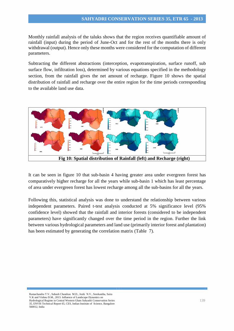
Ramachandra T.V., Subash Chandran M.D., Joshi N.V., Sreekantha, Saira
V.K and Vishnu D.M., 2013. Influence of Landscape Dynamics on
Hydrological Regime in Central Western Ghats Sahyadri Conservation Series
35, ENVIS Technical Report 65, CES, Indian Institute of Science, Bangalore
560012, India
139
SAHYADRI CONSERVATION SERIES 35, ETR 65 - 2013
Monthly rainfall analysis of the taluks shows that the region receives quantifiable amount of
rainfall (input) during the period of June-Oct and for the rest of the months there is only
withdrawal (output). Hence only these months were considered for the computation of different
parameters.
Subtracting the different abstractions (interception, evapotranspiration, surface runoff, sub
surface flow, infiltration loss), determined by various equations specified in the methodology
section, from the rainfall gives the net amount of recharge. Figure 10 shows the spatial
distribution of rainfall and recharge over the entire region for the time periods corresponding
to the available land use data.
Fig 10: Spatial distribution of Rainfall (left) and Recharge (right)
It can be seen in figure 10 that sub-basin 4 having greater area under evergreen forest has
comparatively higher recharge for all the years while sub-basin 1 which has least percentage
of area under evergreen forest has lowest recharge among all the sub-basins for all the years.
Following this, statistical analysis was done to understand the relationship between various
independent parameters. Paired t-test analysis conducted at 5% significance level (95%
confidence level) showed that the rainfall and interior forests (considered to be independent
parameters) have significantly changed over the time period in the region. Further the link
between various hydrological parameters and land use (primarily interior forest and plantation)
has been estimated by generating the correlation matrix (Table 7).

Ramachandra T.V., Subash Chandran M.D., Joshi N.V., Sreekantha, Saira
V.K and Vishnu D.M., 2013. Influence of Landscape Dynamics on
Hydrological Regime in Central Western Ghats Sahyadri Conservation Series
35, ENVIS Technical Report 65, CES, Indian Institute of Science, Bangalore
560012, India
140
SAHYADRI CONSERVATION SERIES 35, ETR 65 - 2013
Table 7: Correlation matrices of different parameters for different years
*Water Yield is sum of surface runoff, interflow and baseflow
In the correlation matrices, values on the right above the diagonal values show the p-value
(significance level) for the null hypothesis stated as the variable are not inter-related. The
values on the left below the diagonal values show the correlation coefficient. The highlighted
values are those that have p-value below 0.05 (5% significance level) for which null hypothesis
can be rejected and the alternate hypothesis stating that the variables are significantly correlated
can be accepted.
From the matrices it can be inferred that interior forests, plantations are strongly positively
correlated to the rainfall. Thus it verifies the rarely documented but often stated fact (LØrup
et. al., 1998) that “forests attract rainfall”. Recharge is also strongly positively related to rainfall
throughout; giving the evidence that groundwater recharge is always dependent on the amount
of rainfall that a region receives. Also there is strong positive relation between interior forests
and infiltration and consequently with recharge for 2006 and 2010 implying that core/pristine
forests promote percolation of water into sub surface system and thus ground water recharge.
Plantations also have shown positive correlation with the recharge throughout the time period.
In addition, for all the years, runoff has shown negative correlation with the interior forests and
positive with plantations inferring that the deep roots of the forests prevent surface runoff while
plantations having shallow rooting system lack that capability. As a consequence, plantations
were found to have strong positive relation with the water yield (dominated by runoff) obtained
from the system.
On plotting land use with individual hydrological parameter (figure 11), it was observed that
the sub-basins having greater proportion of area under Interior forest have higher rainfall, lesser
runoff but higher interflow which contribute to greater water yield (sum of surface runoff,
interflow and baseflow) from such sub-basins. Baseflow was found to be higher for the sub-
basin 5 in comparison to other sub-basins due to higher specific yield of the Greywacke rock
type.

Ramachandra T.V., Subash Chandran M.D., Joshi N.V., Sreekantha, Saira
V.K and Vishnu D.M., 2013. Influence of Landscape Dynamics on
Hydrological Regime in Central Western Ghats Sahyadri Conservation Series
35, ENVIS Technical Report 65, CES, Indian Institute of Science, Bangalore
560012, India
141
SAHYADRI CONSERVATION SERIES 35, ETR 65 - 2013
Fig. 11: Relationship between Rainfall and Runoff (a); Interior forest, Runoff, Interflow
and Base flow (b); Rainfall, Interior forest and Water Yield (c) and Interior forest,
Rainfall, Runoff and Recharge (d)
4.5 Water Balance Analysis
Water balance is analysis done with respect to the demand and supply of water to understand
the deficit and surplus water. The main stakeholders considered for this analysis are population
of the region, livestock, agriculture area to be irrigated and areca plantations (Fig. 12 and Fig.
13). Table 8 shows that, for the entire watershed area, available water was surplus in 2010.
Fig. 12(a) Number of household in a village, (b) Population density of each village
Fig. 13 (a) Water requirement of (a) human population, (b) livestock

Ramachandra T.V., Subash Chandran M.D., Joshi N.V., Sreekantha, Saira
V.K and Vishnu D.M., 2013. Influence of Landscape Dynamics on
Hydrological Regime in Central Western Ghats Sahyadri Conservation Series
35, ENVIS Technical Report 65, CES, Indian Institute of Science, Bangalore
560012, India
142
SAHYADRI CONSERVATION SERIES 35, ETR 65 - 2013
Table 8: Water Balance for the year 2010
4.6 Sustainability of the catchment yield
Irrigation water requirement for the non-monsoon season was computed for each sub-basin for
the year 2010 and compared with the water yield (only interflow and baseflow, as they are
responsible for the non-monsoon flow in the stream) in the sub-basin. Figure 14 shows that the
sub-basin 4 and 5 having greater proportion of area under interior forest have very high water
yield in comparison to the irrigation requirement, while sub-basin 1 and 2 having negligible
area under interior forest has very less water yield. Due to excessive water yield in the sub-
basins 4 and 5, the streams are perennial here while the streams of sub-basins 1 and 2 get dry
after the cessation of monsoon, which has been verified through field visits as well.
Table 9: Irrigation requirement at the sub-basin level in 2010
Sub-
basin
Arecanut Paddy Interior
forest
Net
Irrigation
Requirement
Water
Yield
Area
(sq.km.)
Area
(sq.m.)
Water
requirement
(Mm3)
Area
(sq.km.)
Area
(sq.m.)
Water
requirement
(Mm3)
Area
(sq.km.)
(Mm3) Pre and
Post
Monsoon
(Interflow
and
Baseflow)
(Mm3)
Sub
basin1 13.13 13130000 15.756 30.92 30920000 23.19 0.71 38.946 23.14
Sub
basin2 16.59 16590000 19.908 10.54 10540000 7.905 7.90 27.813 44.71
Sub
basin3 21.60 21600000 25.92 5.98 5980000 4.485 50.31 30.405 158.91
Sub
basin4 31.49 31490000 37.788 18.00 18000000 13.5 121.14 51.288 207.32
Sub basin5
57.37 57370000 68.844 18.18 18180000 13.635 63.54 82.479 304.98
Sub
basin6 28.57 28570000 34.284 21.64 21640000 16.23 34.09 50.514 176.14
Sub
basin7 40.55 40550000 48.66 27.33 27330000 20.4975 55.74 69.1575 260.49
Total
Water
Yield for
the year
2010
(Mm3)
Water requirement by the stakeholder
Human beings Livestock Arecanut Plantation Paddy Net water
requirement
in the region
(Mm3)
Net
water
balance
(Mm3)
Total
No.
Water
requirem
ent
(Mm3/yr)
Total
No.
Water
Requireme
nt
(Mm3/yr)
Area
(m2)
Water
requireme
nt (Mm3)
Rice
productio
n (kg)
Water
requireme
nt (Mm3)
1112.
4
308,
362
11.26 262,
330
6.70 209280
000
251.136 132600
000
99.45 368.456 743.
944

Ramachandra T.V., Subash Chandran M.D., Joshi N.V., Sreekantha, Saira
V.K and Vishnu D.M., 2013. Influence of Landscape Dynamics on
Hydrological Regime in Central Western Ghats Sahyadri Conservation Series
35, ENVIS Technical Report 65, CES, Indian Institute of Science, Bangalore
560012, India
143
SAHYADRI CONSERVATION SERIES 35, ETR 65 - 2013
Fig. 14: Water Budget at the sub-basin level for 2010
5. Conclusion
From the analysis, done to assess the effect of land use on water resources in the region in non-
experimental (empirical) way, it can be concluded that the status of landscape has significant
effect on controlling the water availability in the region. The results obtained show that, whilst
the overall percentage of interior forest in the catchment has shrunk since 1972, still the sub-
basins having relatively greater proportion of area under interior forest have greater water yield
in comparison to sub basins with fragmented forest. Furthermore, from the correlation analysis
it was established that pristine forests have lesser surface runoff and higher groundwater
recharge that result in higher low flows. As a consequence, the streams are perennial in such
regions. In addition, water balance analysis shows that catchment yield of only those sub-basins
is sustainable that have greater proportion of area under interior forest. Thus landscape
structure has much important role in determining the water resources in the region, rather than
just acting as a driver of hydrological cycle.
References
Anderson, H.W., Hoover, M.D. and Reinhart, K.G. 1976, ‘Forest and water: Effects of Forest
Management on Floods, Sedimentation and Water Supply’, Forest service’s Technical Report
RSW-18, Berkley, U.S. Department of Agriculture.
Bithell, M., and Brasington, J. 2009, ‘Coupling agent-based models of subsistence farming
with individual-based forest models and dynamic models of water distribution’, Environmental
Modelling& Software, Vol. 24, pp. 173-190.
Bosch, J.M. and Hewlett, J.D. 1982, ‘A Review of Catchment Experiments to Determine the
Effects of Vegetation Changes on water Yield and Evapotranspiration’, Journal of Hydrology,
Vol. 55, pp. 3-23.
Breuer, L., Huisman, J.A., Willems, P., Bormann, H., Bronstert, A., Croke, B.W.F., Frede,
H.G.,Graff, T., Hubrechts, L., Jakeman, A.J., Kite, G., Lanini, J., Leavesly, G., Lettenmaier,
D.P., Lindstorm, G., Seibert, J., Sivapalan, M. and Viney, N.R. 2009, ‘Assessing the impact

Ramachandra T.V., Subash Chandran M.D., Joshi N.V., Sreekantha, Saira
V.K and Vishnu D.M., 2013. Influence of Landscape Dynamics on
Hydrological Regime in Central Western Ghats Sahyadri Conservation Series
35, ENVIS Technical Report 65, CES, Indian Institute of Science, Bangalore
560012, India
144
SAHYADRI CONSERVATION SERIES 35, ETR 65 - 2013
of land use change on hydrology by ensemble modelling (LUCHEM) I: Model
intercomparison with current land use’, Advances in Water Resources, Vol. 32, pp. 129-146.
Bruijnzeel, L.A. 1989, ‘(De)forestation and dry season flow in the tropics’, Journal of Tropical
Forest Science, Vol. 1, No. 3, pp. 229-243.
Bruinzeel, L.A. 2001, ‘Forest Hydrology’ in Evans, J (ed.) The Forest Handbook, Vol. 1,
Blackwell science, Oxford, UK.
Burel, F and Baudry, J. 2004, ‘Landscape Ecology: Concepts, Methods, Applications, Science
Publishers, New hampshire, U.S.A.
DeFries, R. And Eshleman, K.N. 2004, ‘Land-use change and hydrologic processes: a major
focus for the future’, Hydrological Processes, Vol. 18, pp. 2183-2186.
Dunne, T and Leopold L.B. 1978, ‘Water in environmental planning’, W.H. Freeman and Co.,
New York.
Forman, R and Godron, M. 1986, Landscape Ecology, John Wiley and Sons, New York, U.S.A.
Gretchen, C.D. 1995, ‘Restoring value of the world’s degraded lands’, Science, Vol. 269, pp.
350-354.
Guoquing, W & Hui, Y 2005, ‘Study on Hydrologic Simulation of Qingjianhe River Basin in
the Middle Yellow River’ Proceedings of IIASA-DPRI.
Hibbert, A.R. 1967, ‘Forest treatment effects on water yield’, in Sopper, W.E. and Lull, H.W.
(eds.) International Symposium on Forest Hydrology, pp. 527-543, Permagon Press, New
York.
Hobbs, N.T., Galvin, K.A., Stokes, C.J., Lackett, J.M., Ash, A.J., Bonne, R.B., Reid, R.S and
Thornton, P.K. 2008, ‘Fragmentation of rangelands: Implications for humans, animals and
landscape’, Global Environmental Change, Vol. 18, pp.776-785.
Hurd, J. and Civco, D. 2008, ‘Assessing the impact of Land Cover Spatial Resolution on Forest
Fragmentation Modeling’, ASPRS 2008 Annual Conference, Portland, Oregon, April 28 – May
2, 2008.
Hurd, J., Wilson, E. and Civco, D. 2002, ‘Development of Forest Fragmentation Index to
Quantify the Rate of Forest Change’, ASPRS-ACSM 2002 Annual Conference and FIG XXII
onference, April 22 – 26, 2002.
Hurd, J., Wilson, E., Lammey, S. and Civco, D. 2001, ‘Characterization of Forest
Fragmentation and Urban Sprawl using Time Sequential Landsat Imagery’, ASPRS 2001
Annual Conference, St. Louis, MO, April 23-27, 2001.
Leopold, L.B. 1968, ‘Hydrology for urban land planning- a guidebook on the hydrologic effects
of urban land use’, U.S. Geological Survey Circular 554.

Ramachandra T.V., Subash Chandran M.D., Joshi N.V., Sreekantha, Saira
V.K and Vishnu D.M., 2013. Influence of Landscape Dynamics on
Hydrological Regime in Central Western Ghats Sahyadri Conservation Series
35, ENVIS Technical Report 65, CES, Indian Institute of Science, Bangalore
560012, India
145
SAHYADRI CONSERVATION SERIES 35, ETR 65 - 2013
Lerner, D.N. and Harris, B. 2009, ‘The relationship between land use and groundwater
resources and quality’, Land Use Policy, Vol. 26S, pp. S265-S273.
Lin, Y.P., Hong, N.M., Wu, P.J., Wu, C.F. and Verburg, P.H. 2007, ‘Impacts of land use change
scenarios on hydrology and land use patterns in the Wu-Tu watershed in Northern Taiwan,
Landscape and Urban Planning, Vol.80, No.1-2, pp. 111-126.
LØrup, J.K., Refsgaard, J.C. and Mazvimavi, D. 1998, ‘Assessing the effect of land use change
on catchment runoff by combined statistical tests and hydrological modeling: Case studies from
Zimbabwe’, Journal of Hydrology, Vol. 205, pp. 147-163.
Mutreja, K.N. 1986, Applied Hydrology, Tata Mc Graw Hill, New Delhi.
Paulson, D.D. 1994, ‘Understanding tropical deforestation: A case of western Samao’,
Environmental Conservation, Vol. 21, pp. 326-332.
Purandara, BK, Venkatesh B & Choubey VK 2010, ‘Estimation of Groundwater Recharge
under various land covers in parts of Western ghats, Karnataka, India’, Material and
Geoenvironment, Vol. 57, No. 2, pp. 181-194.
Putty, M.R.Y and Prasad, R. 2004, ‘Understanding runoff processes using a watershed model-
a case study of Western Ghats in South India’, Journal of Hydrology, Vol. 228, pp. 215-227.
Raghunath, H.M. 1985, Hydrology: Principles, Analysis, Design, Wiley Eastern Limited, New
Delhi, India.
Ramachandra, T.V., Kumar, U., Diwakar, P.G. and Joshi, N.V. 2009, ‘Land Cover Assessment
using À Trous Wavelet fusion and K-Nearest Neighbour classification’, Proceedings of the
25th Annual In-House Symposium on Space Science and Technology, ISRO-IISc Space
Technology Cell, Indian Institute of Science, Bangalore, 29-30 January 2009.
Ramachandra, T.V., Subhash Chandran, M.D., Sheekantha, Mesta, D., Rao, G.R. and Ali, S.
2004, ‘Cumulative Impact Assessment in the Sharavathi River Basin’, International Journal
of Environment and Development, Vol. 1, No.1, pp. 113-135.
Rattanaviwatpong, P., Richey, J., Thomas, D., Rodda, S., Campbell, B. and Logsdon, M. 2005,
‘Effects of landuse change on the hydrologic regime of Mae Chaem river basin, NW Thailand’,
submitted in Journal of Hydrology.
Ritters, K., Wickham, J., O’Neill, R., Jones, B. and Smith, E. 2000, ‘Global-Scale Patterns of
Forest Fragmentation’, Conservation Ecology, Vol. 4, No. 2, Article 3.
Ruder, T and Roper, J. 1996, ‘Regional pattern and historical trends in tropical deforestation,
1976-1990: A qualitative comparative analysis, Ambio, Vol. 25, pp. 160-166.
Sano, E.E., Huete, A.R., Troufleau, D., Moran, M.S. and Vidal, A. 1998, ‘Relation between
ERS-1 synthetic aperture radar data and measurement of surface roughness and moisture
content of rocky soils in a semiarid rangeland’, Water Resources Research, Vol. 34, pp.
1491-1498.

Ramachandra T.V., Subash Chandran M.D., Joshi N.V., Sreekantha, Saira
V.K and Vishnu D.M., 2013. Influence of Landscape Dynamics on
Hydrological Regime in Central Western Ghats Sahyadri Conservation Series
35, ENVIS Technical Report 65, CES, Indian Institute of Science, Bangalore
560012, India
146
SAHYADRI CONSERVATION SERIES 35, ETR 65 - 2013
Schulze, R.E. 2000, ‘Modelling Hydrological Responses to Land Use and Climate Change: A
Southern African Perspective’, Ambio, Vol. 29, No. 1, pp. 12-22.
Schwartz, F. and Zhang, H. 2003, Fundamentals of Ground Water, John Wiley and Sons, New
York, U.S.A.
Scott, D.F. and Lesch, W. 1997, ‘Streamflow responses to afforestation with Eucalyptus
grandis and Pinus patula and to felling in the Mokobulaan experimental catchments, South
Africa, Journal of Hydrology, Vol. 199, No. 3-4, pp. 360-377.
Shuttleworth, W.J. 1993, ‘Evapotranspiration’ in Maidment, D.R. (ed.) Handbook of
Hydrology, McGraw Hill Publication, U.S.A.
Sikka, A.K., Samra, J.S., Sharda, V.N., Samraj, P and Lakshman, V. 2003, ‘Low flow and high
flow responses to converting natural grassland into blue gum (Eucalyptus globulus) plantation
in Nilgiris watersheds of South India, Journal of Hydrology, Vol. 270, No. 1-2, pp. 12-26.
Singh, V.P. 1994, Elementary Hydrology, Prentice Hall of India, New Delhi, India.
Slonecker E., Jennings, D. and Garofalo, D., 2001, ‘Remote Sensing of impervious surfaces:
a review’, Remote Sensing Reviews, Vol. 20, pp. 227-255.
Smith, J.A., Baeck, M.L.Steiner, M. and Miller, A.J. 1996, ‘Catastrophic rainfall from an
upslope thunderstorm in the central Appalachians: the Rapidan storm of June 27, 1995’, Water
Resources Research, Vol. 32, pp. 3099-3113.
Sturdevant-Rees, P., Smith, J.A., Morrison, J. and Baeck, M.L. 2001, ‘Tropical storms and the
flood hydrology of the central Appalachians’, Water Resources Research, Vol. 37, pp. 2143-
2168.
Subramanya, K. 2008, Engineering Hydrology, 3rd edition, Tata McGraw Hill Education
Private Limited, New Delhi, India.
Townsend, P.A.and Foster, J.A. 2002, ‘A SAR-based model to assess historical changes in
lowland floodplain hydroperiod’, Water Resources Research, Vol. 38, No. 7, DOI: 10-
1029/2001WR001046.
Turner II, B.L., Matson, P.A., McCarthy, J., Corell, R.W., Christensen, L., Eckley, N.,
Hoverlsrud_Broda, G.K., Karperson, J.X., Karperson, R.E., Luers, A., Martello, M.L.,
Matheisen, S., Naylor, R., Polsky, C., Pulsipher, A., Schiller, A., Selin, H. And Tyler, N. 2003,
‘Illustrating the coupled human-environment system for vulnerability analysis: three case
studies’, Proceedings of the National Academies of Sciences, Vol. 100, No. 14, pp. 8080-8085.
Turner, M.G., Gardner, R.H. and O’Neill, R.V. 2001, Landscape Ecology, In Theory and
Practice, Pattern and Process, Springer-Verlag, New York, U.S.A.
Van Lill, W.S., Kruger, F.J. and Van Wyk, D.B. 1980, ‘The effect of afforestation with
Eucalyptus grandis Hill ex Maiden and Pinus patula Schlecht. et Cham. on streamflow from

Ramachandra T.V., Subash Chandran M.D., Joshi N.V., Sreekantha, Saira
V.K and Vishnu D.M., 2013. Influence of Landscape Dynamics on
Hydrological Regime in Central Western Ghats Sahyadri Conservation Series
35, ENVIS Technical Report 65, CES, Indian Institute of Science, Bangalore
560012, India
147
SAHYADRI CONSERVATION SERIES 35, ETR 65 - 2013
experimental catchments at Mokobulaan, Transvaal, Journal of Hydrology, Vol. 48, No. 1-2,
pp. 107-118.
Zeigler, A.D., Giambelluca, T.W., Tran, L.T., Vana, T.T., Nullet, M.A., Fox, J., Vien, T.D.,
Pinthong, J., Maxwell, J.F. and Evett, S. 2004, ‘Hydrological consequences of landscape
fragmentation in mountainous northern Vietnam: evidence of accelerated overland flow
generation’, Journal of Hydrology, Vol. 287, pp. 124-146.

148
SAHYADRI CONSERVATION SERIES 35, ETR 65 - 2013
Appendix I - Vegetation Characteristics of Western Ghats Type of
vegetation
Species Type of
roots
Root depth (m) Description of roots Crown shape Leaf /
leaflet/
shape
Evergreen Mangifera
indica
Shallow
to deep
tap root
5.5 (Stephens, 1949)
1.2 (Musahibuddin, 1960)
Almost the level of
water table in
Queensland (Australia)
Spherical/ broad Oblong
Cocos
nucifera
Fibrous
roots
4-6 (Ramadasan and
Rajagopal, 1987)
Palm, upright Linear
lanceolate
Tamarindus
indica L.
Moderat
ely deep
taproot
1.5 (minimum)
http://plants.usda.gov/cgi_b
in/char_sciname.cgi
Spherical Ovate
lanceolate
Delonix
regia
(Gulmohar
tree)
Moderat
ely deep
taproot
1.5 (minimum)
http://plants.usda.gov/cgi_b
in/char_sciname.cgi
Spreading, vase shape,
Flat crowned (umbrella
shaped)
Oblong
Michelia
champaca
Deep tap
root
Requires moist deep
soil (Troupa, 1986)
Rounded Ovate
lanceolate
Polyalthia
fragrans
Buttress
roots
(Troupa, 1986) Conical Lanceolate
ovate
Mesua
ferrea
Taproot Seedling roots: primary
root moderately long,
lateral roots numerous,
long, fibrous and
Rounded Elliptical
lanceolate

149
SAHYADRI CONSERVATION SERIES 35, ETR 65 - 2013
branched (Troupa,
1986)
Dipterocarp
us indicus
Buttress
roots
Seedling roots: primary
root long, lateral roots
short and distributed
down main root
(Troupa, 1986)
Rounded Ovate
Pterospermu
m
acerifolium
Taproot Seedling root: Primary
root long, lateral roots
numerous, fine and
distributed down main
root (Troupa, 1986)
Conical Ovate
Azadirachta
indica
Taproot Seedling root: Primary
root moderately long
(Troupa, 1986)
Spreading, rounded Ovate
lanceolate
Hardiwickia
pinnata
Taproot Seedling root: primary
root long, lateral roots
few to moderate in
number
(Troupb, 1986)
Rounded Oblong
Santalum
album
Taproot Seedling root: primary
root long, flexuous,
whitish delicate, lateral
roots moderate in
number, distributed
down main root. Roots
at an early stage show
Elliptical

150
SAHYADRI CONSERVATION SERIES 35, ETR 65 - 2013
nodular growths, the
first signs of haustoria.
(Troupc 1986)
Deciduous Terminalia
catappa
Shallow
taproot
0.82 (minimum)
http://plants.usda.gov/cgi_b
in/char_sciname.cgi
Broad, flat Obovate
oblanceolat
e
Albizzia
lebbek
Shallow
to
moderat
ely deep
tap root
0-1.4
1.4-2.05
>2.05
(Muthana et al. 1984)
Sand to loamy sand,
loose friable
Gravelly loamy sand,
somewhat compact
Hard compact zone,
rich in lime
Moderately spreading,
feathery
Oblong
Dalbergia
sisoo
Shallow
tap root
1 (Chaulya et al. 2000) Obovate/or
bicular
Terminalia
tomentosa
Deep tap
root
3.6
Champion and Trevor,
(1938)
Attained 3.6 m in two
growing seasons
Oblong
Bombax
malabaricu
m
Buttress
roots
Seedling root: Primary
root long, lateral roots
few or moderately
numerous
(Troupa, 1986)
Elliptical, elongated Ovate or
cordate
Aegle
marmelos
Tap root Seedling root: Primary
root long, lateral roots
few or moderate in
number and distributed
down the main root.
Round Elliptical
lanceolate

151
SAHYADRI CONSERVATION SERIES 35, ETR 65 - 2013
Root system is
superficial. Lateral
roots spreads to some
distance
(Troupa, 1986)
Acrocarpus
fraxinifolius
Large
buttress
roots
Seedling roots: Primary
root moderately long,
lateral root moderate in
number and length
(Troupa, 1986)
Rounded Elliptical
lanceolate
Cassia
fistula
Tap root Seedling roots: primary
root long, lateral roots
numerous, fibrous,
distributed down main
root
(Troupb, 1986)
Open crown Ovate
oblong
Xylia
xylocarpa
Tap root Seedling roots: primary
root long, lateral roots
fairly numerous, long
and distributed down
main roots
(Troupb, 1986)
Elliptical

152
SAHYADRI CONSERVATION SERIES 35, ETR 65 - 2013
Anogeissus
latifolia
Tap root Seedling roots: Primary
root long, lateral roots
few to moderate in
number, short, fibrous
and distributed down
main root
(Troupc, 1986)
Feathery and rounded
Plantations Acacia
catechu
Deep tap
root
2
(http://www.deh.gov.au/bio
diversity/invasive/publicati
ons/a-catechu.html)
Rounded
Eucalyptus
globulus
Deep tap
root
2.8
Samraj et al. (1977)
Elongated Lanceolate
Eucalyptus
hybrid
Shallow
to
moderat
ely deep
taproot
1.5-2
>2
Rajan, (1980)
Nandi Hills
Lanceolate
Tectona
grandis
Shallow
taproot
0.3-0.4 Singh et al (1984)
< 0.5
http://library.wur.nl/prosro
m/tectona.html
The primary root is
long, but gradually
disappears after lateral
roots have developed
Spreading, conical Obovate

153
SAHYADRI CONSERVATION SERIES 35, ETR 65 - 2013
Casuarina
equisetifolia
Shallow
taproot
0.6 minimum
(http://plants.usda.gov/cgi_
bin/char_sciname.cgi)
Elongated Narrowly
angular
Hevea
brasliensis
Very
deep tap
root
> 10 (Moraes, 1977)
In shallow alluvial
soils, tap roots are
confined to the top
zone of A horizon but
are compensated by
profuse growth of
lateral roots
Foliose crown (flat and
thin)
Ovate


