Rainy Day Stocks

Niels Gormsen Robin Greenwood

Working Paper 17-066

Working Paper 17-066

Copyright © 2017 by Niels Gormsen and Robin Greenwood

Working papers are in draft form. This working paper is distributed for purposes of comment and discussion only. It may not be reproduced without permission of the copyright holder. Copies of working papers are available from the author.

Rainy Day Stocks Niels Gormsen Copenhagen Business School

Robin Greenwood Harvard Business School

 

 

Rainy Day Stocks

Niels Gormsen Copenhagen Business School

ng.fi@cbs.dk

Robin Greenwood Harvard Business School

rgreenwood@hbs.edu

January 2017

(First draft April 2016)

Abstract

We study the good- and bad-times performance of equity portfolios formed on characteristics. Many characteristics associated with good performance during bad times – value, profitability, small size, safety, and total volatility – also perform well during good times. Stocks with characteristics signifying high liquidity, such as high turnover and low bid ask spreads, perform well during bad times but otherwise underperform. We develop a simple but flexible procedure to recover a “risk neutral alpha” that recognizes a 1% return experienced during bad times as being more valuable than a 1% return generated during good times. We also show how an investor can build a “rainy day” portfolio that minimizes underperformance during bad times.

Acknowledgments and Disclosures: We thank Kent Daniel, Sam Hanson, Owen Lamont, Ian Martin, Lasse Pedersen, Erik Stafford, Adi Sunderam and Luis Viceira for useful discussions. The authors list all professional activities and potential conflicts on their websites at their home institutions.

‐‐1‐‐  

One of the organizing principles of modern asset pricing theory is that investors should pay

higher prices for securities that pay handsomely in bad times. In the Consumption CAPM, for

example, the price of a risky asset, pt, is determined by the future payoff xt+1, times the rate of time

preference, θ, and the marginal utility of consumption in the period in which the asset pays off:

11

( )

( )t

t t tt

u cp E x

u c

(1)

An equivalent formulation of this idea is that securities that perform well during bad times should

earn low average returns.

However appealing the idea encapsulated by equation (1) may be, it has been of limited

use in explaining the pricing of individual stocks. The simplest measure of a security’s downside

exposure – its CAPM β – has long been known to be insufficient to explain the cross-section of

returns (Black, Jensen and Scholes (1972), Brennan (1971), Fama and French (1992)). Measures

of downside risk based on consumption data have an even poorer record matching the data (Hanson

and Singleton 1982, 1983; Parker 2003; Campbell and Cochrane 2000). Although some

researchers have identified measures of downside exposure that correlate somewhat better with

expected returns, the overall empirical success of the consumption CAPM for the cross-section of

stocks has been limited.1

The Consumption CAPM still, however, serves an important normative purpose: investors

should avoid securities that pay off poorly in bad states of the world, and even more so if those

securities do not handsomely reward investors during ordinary times. In this paper, we embrace

                                                            1 Researchers have had slight success when measuring the correlation of stocks with longer-term consumption growth. However, the resulting measures of bad times do not easily conform to conventional views of what an investor would call bad times (Parker 2001; Bansal and Yaron 2004; Parker and Julliard 2005; Malloy, Moskowitz, Vissing-Jorgensen 2009 and many others). 

‐‐2‐‐  

this normative objective. We ask, for an equity investor who is worried about bad times in the

future, what securities should she optimally hold? And, if this investor holds stocks that are less

exposed to bad times, how much performance drag can such an investor expect? We answer these

questions by adopting a two-state asset pricing model in which times are either good or bad. We

show that adopting this simple approach recasts the performance of many well-known risk factors

in a way that is useful for real-world investors.

Our analysis proceeds in three steps. First, we must settle on a definition of bad times. The

concept of bad times is highly model- and preference-dependent. We adopt the approach of

classifying as bad times periods that would be classified as bad by nearly any sensible

representation of the stochastic discount factor, and would likely be considered as difficult periods

by most investors. Specifically, most of our analysis is performed using a measure that captures

periods of extended stock market drawdown occurring simultaneously with poor economic data.

According to our measure, bad times are quarters with yearly excess market return of minus

nineteen percent, negative GDP and earnings growth, and high inflation and unemployment. While

our two state approach is a simplification of a continuum of states, it is easy to implement because

one does not have to calibrate a utility function.

Second, we identify which types of stocks performed the best during bad times –

professional investors sometimes refer to these stocks as “defensive equities.” We sort stocks into

quintiles based on their total ex post returns during bad times, and measure the characteristics of

the best performing quintile at the start of each bad times episode. A number of distinct patterns

emerge. Defensive stocks score high on value, profitability, “safety”, are growing slowly, have

low volatility and are highly liquid (high turnover and low bid ask spreads). These results only

partly reflect the fact that some of these characteristics are associated with low CAPM betas.

‐‐3‐‐  

Third, guided by the results above, we build long-short portfolios based on characteristics

so as to measure the discount or premium associated with performing well during bad times. For

each of these portfolios, we measure its unconditional market beta, and its conditional good-times

and bad-times alpha. For example, the value factor HML has a CAPM beta of -0.06, a good-times

alpha of 0.32% per month, and a bad times alpha of 1.09% per month. Having both a positive bad-

times alpha and positive good-times alpha is suprising, but appears in many of the characteristics-

based portfolios that we study.

How should an investor assess the state contingent bad times alpha achieved by these

strategies? We propose a simple approach guided by the normative logic of the consumption

CAPM and the pricing of the overall stock market. Namely, if the aggregate stock market is priced

correctly on average, then we can back out the implicit value that investors place on achieving

returns during good and bad times. We then use the implied state prices during good and bad states

to evaluate the realized returns of our characteristic-sorted portfolios. The difference between the

state-price weighted returns across good and bad states yields each strategy’s “risk neutral alpha.”

Our measure is akin to evaluating equity portfolio returns under the risk neutral measure. Our

approach differs from the more standard CAPM alpha, which after controlling for beta, equally

rewards performance in good and bad times. For example, the CAPM implicitly puts the same

value on a loss in December 2008 and a loss in January 2004—both months in which the market

was up by 2.2 percent.

Our analysis yields the following conclusions. Portfolios based on liquidity measures

outperform during bad times but underperform during good times, thus achieving risk neutral

alphas close to zero. For the characteristics of value, and profitability, however, the risk neutral

alphas are even higher than the CAPM alphas, reflecting that these strategies perform even better

‐‐4‐‐  

during bad times than during good times. Finally, low-risk factors have bad-times alphas around

zero, but since they have large good-times alphas they have positive and large risk neutral alphas.

We combine these insights to construct a “rainy day portfolio” that is long stocks that perform well

during bad times: those with high book-to-market, high profitability, and market capitalization

below the median. The rainy day portfolio has an unconditional CAPM alpha of .8 percent per

month and it has a bad times alpha of 2.3 percent per month.

We don’t mean to suggest that our characteristics-based portfolios are the only ways that

an investor can immunize herself against bad times. For example, the most well-known bad-time

protection strategy is to buy out of the money puts on the market index. Applying our two-state

methodology to the profits from this options-based strategy, we show that such a strategy has a

positive good-times alpha and a negative bad times alpha, with a risk neutral alpha close to zero.

This lends some confidence to our classification of good and bad times.

In the last section, we describe a number of extensions and robustness tests. We show that

industries can be easily classified according to their exposure to good and bad times; however,

defensive industries tend to underperform slightly during good times—this effect is subtle as the

correlation between good- and bad-times alpha is only -0.15. We show that the characteristics that

we identify as being robust to bad times among US stocks (size, book-to-market, and profitability)

have similar performance amongst international stocks as well. We also compute risk neutral

alphas using different definitions of bad times and find that our results are largely robust across

the different definitions.

A large literature in asset pricing connects measures of risk to expected returns of

individual stocks or portfolios. A common starting point for many of these papers is the

‐‐5‐‐  

observation that the securities market line – the relationship between average returns and the

CAPM beta – is too flat relative to CAPM theory. A number of papers have developed more

nuanced risk measures to fit the cross-section of returns, starting with Chen, Roll, and Ross’s

(1986) study of exposure to macroeconomic variables. Other studies include Ang, Chen, and Xing

(2006) who analyze stocks’ downside beta, and Parker (2003), Parker and Julliard (2005), Malloy,

Moskowitz, and Vissing-Jorgensen (2009), and Yogo (2006) who study exposure to changes in

consumption.2 Our normative approach departs from the approach taken in most of the literature,

because we do not attempt to fit any particular asset pricing model.

In Section I, we develop simple time-series measures of bad times. In Section II, we

describe the ex-post characteristics of stocks that exhibited the best performance during bad times.

Section III develops a simple procedure to risk adjust portfolio returns for their exposure to bad

times and applies it to characteristic-sorted portfolios in US data 1963-2015. We also develop a

“rainy day” portfolio built to minimize drawdowns in bad times. Section IV describes a number

of extensions. Section V concludes.

                                                            2 For similar approaches, see also Jagannathan and Wang (1996); Heaton and Lucas (2000); Cochrane (1996); Vassalou (2003); Li, Vassalou, and Xing (2006); Ait-Sahalia, Parker, and Yogo (2004); Bansal, Dittmar, and Lundblad (2005); Hansen, Heaton, and Li (2006); Campbell and Vuolteenaho (2004). Lewellen, Nagel, and Shanken (2010) and Daniel and Titman (2012) offer a skeptical view on these approaches.

‐‐6‐‐  

I. Identifying Bad Times

Bad times are periods where investors place a high value on investment payoffs. Asset

pricing has admitted several definitions of bad times, which depend on the specification of

investors’ utility function. Intuitively, bad times may be when the economy is troubled and

investors face a higher risk of job loss or reduced wages and have to reduce consumption as a

result, or it may be when financial markets are troubled and investors have realized large financial

losses. In the Sharpe-Lintner CAPM, states of the world are fully summarized by the return on the

aggregate financial wealth portfolio. Consumption based models suggest that bad times are periods

where the economy is troubled, or aggregate consumption has fallen (Lucas (1978), Breeden

(1979) Campbell and Cochrane (2000)). To encompass the largest class of theoretical models, our

baseline measure of bad times is when the economy is experiencing both economic and financial

bad times.

We define financial bad times as quarters in which either the quarterly or the yearly US

stock market excess return is in the bottom quintile of our sample, which runs from 1963 to 2013.

By evaluating yearly excess returns as well as shorter-term quarterly returns, we ensure that we

identify as bad times periods when the market is in a large drawdown, even if there has been a

partial recovery. Specifically, if the market drops dramatically in one quarter, and neither recovers

nor worsens in the following quarter, then this following quarter is likely to be defined as financial

bad times despite having neither high nor low returns itself.

To define economic bad times, we use the NBER business cycle indicator. We define a

quarter to be economic bad times if at least one of its months is registered as a recession by the

‐‐7‐‐  

NBER. Our resulting classification of quarters into economic bad times is similar if we instead use

industrial production or annual real GDP growth and select the bottom quintile in the time series.

We define the rainy day index as a quarterly dummy variable equal to one if the quarter

has both economic and financial bad times and zero otherwise. While this restrictive definition

may leave out some periods that would be admitted as a bad time under some specifications, our

approach minimizes false positives. Figure 1 shows the time-series of the rainy day index.

Table 1 reports sample average of different economic and financial variables under

different definitions of bad times. The first column shows the economic and financial features of

our entire sample, and the remaining columns show the averages during different definitions of

bad times. Rainy days are worse than normal times on nearly all dimensions: annualized excess

market returns of minus nineteen percent, year-on-year GDP growth of minus one percent,

earnings growth of minus twenty-five percent, higher than average inflation, higher than average

unemployment, and a five percent yearly drop in home prices. Rainy days are also associated with

a higher TED spread, a higher market volatility as proxied by the VIX, and more noise in the term

structure as captured in Hu, Pan, and Wang’s (2013) term structure noise measure.3 Rainy days

indeed appear to capture difficult times for almost any investor. Our rainy day index is strongly

negatively correlated with growth of durable consumption, but uncorrelated with nondurable

consumption.

We noted that our measure of financial bad times includes some of the rebound period after

a stock market crash, when the market is still down significantly from peak. Table 1 also describes

                                                            3 TED spreads, VIX, and the noise measure are not available for the complete time-series.

‐‐8‐‐  

a measure of bad times called “drawdown” that excludes the rebound period.4 “Drawdown” bad

times are quite similar to our baseline measure of financial bad times, however the market returns

are somewhat lower.

Finally, while most of our discussion will center on the performance of US stocks during

bad times, as a robustness check, we also perform our analysis on a global sample of stocks from

1986-2013. We construct a separate rainy day index for the global sample. We use the excess

return to the global value-weighted market portfolio to construct our global financial bad times.

We define global economic bad times as the periods where the growth in GDP for OECD countries

is in the bottom quintile of the sample. As presented in Table 1, the features of the global rainy

days are quite similar to the U.S. rainy days. Further, the correlation between the global rainy days

and the U.S. rainy days is 0.82.

II. Which Stocks Outperform during Bad Times?

To identify rainy day stocks, we first sort stocks into portfolios based on their ex-post

performance during rainy days. We then calculate the ex ante characteristics of the portfolios and

look for relationship between characteristics and returns.

We include the following characteristics in our analysis: market value, book-to-market,

momentum, profitability, “growth”, “safety”, total volatility, turnover, modified Amihud ratio5,

and the bid-ask spread. As our profitability, growth, and safety measures we use the composite

                                                            4 The column labelled “drawdown” considers all market drawdowns with peak below minus ten percent: bad times are defined as the period between the beginning and the maximum of the drawdown period. We set the maximum length of a drawdown to be five years.  5 We estimate Amihud ratios as suggested by Amihud (2002) except that we base our measures on turnover rather than raw volume, so as not to mechanically confound liquidity with size.

‐‐9‐‐  

variables defined by Asness, Frazzini, and Pedersen (2014).6 We update accounting information

each June using information from the end of December in the previous year. We update market

capitalization at the end of each month. Our choice of characteristics is guided by prior research.

Characteristics can loosely be grouped into those related to fundamentals (size, profitability, safety

and total volatility, and growth), past price movements (momentum), and liquidity factors

(Amihud ratios, turnover, and bid-ask spreads). Many of these characteristics are known to

produce unconditional alphas, but this is not a prerequisite for inclusion. Our primary focus here

is on when these alphas are produced.

We group consecutive quarters of bad times into a total of seven periods (1969Q4-1970Q3;

1973Q4-1975Q1; 1980Q4; 1981Q3-1982Q2; 1990Q3-Q4; 2001Q1-Q4; 2008Q1-2009Q2). For

each of the seven periods, we sort the stocks into quintiles based on the ex post return over the full

bad times period, where the breakpoints are based on the ex post return to NYSE firms. Within

each quintile, we calculate the equal weighted ex ante characteristics of each portfolio. This

procedure results in seven periods with five portfolios in each. Our final characteristics estimate

for each of the five portfolios is the average across the seven periods.7 We measure characteristics

as the cross-sectional percentile.

Panel A of Table 2 shows these results. The best performing quintile of stocks

disproportionately contains value, safety, low growth, low total volatility, high Amihud ratios (i.e.,

illiquid), and low turnover. These results reflect, at least in part, the fact that some of the

characteristics we examine are correlated with CAPM betas. Thus, in Panel B we instead sort

                                                            6 We estimate the modified Amihud ratio, turnover, and bid-ask spreads using daily data over 90 days. We require at least 30 observations to construct the characteristic. Bid-ask spreads are closing spreads which are available on CRSP from 1982 for NASDAQ firms and 1992 for NYSE/AMEX firms. 7 The time-series weights are the number of quarters each consecutive period of rainy days last.

‐‐10‐‐  

stocks on CAPM alphas realized during bad times. For each period, we compute alphas as the

cumulative excess return to the stock minus its ex ante beta times the cumulative excess return to

the market. We estimate the betas in the same way as Frazzini and Pedersen (2014).8Adjusting for

market beta has the effect of reducing the overrepresentation of growth and total volatility among

the groups of the best performing stocks. Adjusting for market beta also changes the conclusion

about the liquidity characteristics, as the best performing stocks are now associated with high

liquidity (high turnover and low bid ask spreads). Aside from that, the characteristics that perform

well during bad times in Panel A seem to also be associated with CAPM alpha.

While these results suggest that equity investors may be able to hedge against bad times by

holdings stocks with particular characteristics, the results are ex post and thus do not provide much

quantitative guidance as to how effectively an investor could protect himself against bad times ex

ante, and the results do not offer insight into the price investors must pay during good times for

this bad times protection. We present formal tests in the next section.

III. Measuring the Performance of Rainy Day Stocks

We now describe the returns of portfolios based on the characteristics in Section II. We

follow Fama and French and construct our factors as the intersection of six value-weighted

portfolios formed on size and the portfolio’s characteristic.9 The turnover factor, for instance, is

                                                            8 We shrink the estimated betas towards their cross-sectional mean, 1 , with shrinkage factor

0.6 and cross-sectional mean 1.Our estimates of betas are given by , , where and are

the estimated volatilities of stock and the market and , is their correlation. We use five-year rolling windows and overlapping three-day log returns, , ∑ ln 1 , to estimate correlation. We use one-year rolling windows and one-day log returns to estimate volatilities. We require at least 750 trading days of non-missing return data to estimate correlation and 120 trading days of non-missing return data to estimate volatility. 9 We use the size and momentum factors from Fama and French, the value factor from Asness and Frazzini (2013), and the safety, profitability, and growth factor from Asness, Frazzini, and Pedersen (2013). 

‐‐11‐‐  

long half a dollar in each of the two high turnover portfolios and short half a dollar in each of the

two low turnover portfolios. We use conditional sorts for the portfolio breakpoints. We follow the

convention that the long side of the portfolio buys the stocks that have high unconditional CAPM

alpha, which is not necessarily the same as having a high alpha during bad times.

The first two rows of Panel A of Table 3 summarize average excess monthly returns during

good and bad times. Value, profitability, safety, total volatility, and turnover-sorted portfolios

outperform by more than 50 basis points per month during bad times, although the performance is

only statistically significant in the case of value and profitability.

As in Section II, the results on excess returns partially reflect differential exposure of these

long short portfolios to the stock market. To control for this exposure, we regress portfolio excess

returns ,eptr on the aggregate stock market excess return and a bad times dummy:

,e 1 ( )p m ft u b b t tr r r u (2)

Notice that we estimate a single beta in equation rather than separate good and bad times betas.

The idea behind a constant beta is that it captures a simple market hedge achievable ex ante, even

if bad times are not forecastable.10

Equation (2) measures the conditional performance of an investor who shorts β units of the

market as a hedge. The return this investor achieves during good times is estimated as αu, while

the bad times performance is given by the sum αu+ αb. Panel B of Table 3 shows these results.

Column (1) shows that the Fama-French SMB portfolio, that buys small stocks and sells short

                                                            10  If states are defined only by market returns, then the statement that a portfolio has a high bad times alpha is equivalent to saying that it has a higher downside beta. This no longer holds exactly when bad times are defined based on variables other than the market return. 

‐‐12‐‐  

large stocks, has a good times alpha of 0.18 percentage points per month, and a beta of 0.19. In

addition, small stocks earn an additional 0.27 percentage points per month in alpha during bad

times, thus totaling 0.45 percentage points per month.

The value portfolio has a good times alpha of 0.32 percentage points per month, and a bad

times alpha of 1.09 percentage points per month. Profitable stocks have a good times alpha of 0.25

basis points per month, and a bad times total alpha of 0.43 percentage points. Growth stocks,

however, outperform during good times but underperform during bad times. “Safe” and low

volatility stocks outperform (on a beta adjusted basis) during good times, and underperform

modestly during bad times. Momentum exhibits enormous outperformance during good times

(0.89 percentage points per month) but underperforms during bad times. The various

characteristics measuring illiquidity – Amihud, low turnover and high bid-ask – all outperform

during good times but underperform during bad times.

The main takeaway from this table is that for many characteristics that are associated with

an unconditional alpha, this does not come at the expense of performance during bad times.

Similarly, outperformance during bad times is not associated with any discount in good times.

There are some characteristics, however, for which outperformance in bad times is associated with

underperformance during good times. In particular, illiquid portfolios (high Amihud ratios, low

turnover, high bid-ask spreads) all earn an alpha during good times, but pay for it with

underperformance during bad times. Low turnover stocks, for example, achieve a good times alpha

of 0.40 percentage points per month, but bad times performance is -0.22 percentage points per

month.

Computing Risk Adjusted Performance

‐‐13‐‐  

Although our conditional bad times alpha estimates are revealing, their magnitude is

difficult to evaluate without a benchmark of how much outperformance in bad times should be

equated with underperformance in good times (or conversely). For example, columns (5) and (7)

show that safety and momentum underperform slightly during bad times, but on the other hand

they experience large outperformance during good times.

Consider the stochastic discount factor representation of asset prices. For any portfolio p

that is correctly priced:

,e0 pE mr (3)

in which and m denotes the stochastic discount factor, and ,epr is the return to portfolio p net of

the risk free rate. If there are only two states good (g) and bad (b), it then follows that:

,e

,e.

mg gb

mg b b

rm

m r

(4)

where s denotes the probability of state s.

To go from a ratio of state prices to the level, we make use of the fact that

1/ (1 ) [ ] .fb b g gr E m m m (5)

This allows us to solve for state prices

‐‐14‐‐  

,e

,e

,e

,e

1 / (1 )

1/ (1 )

f

b mb

b bmg

f

g mg

g gmb

rm

r

r

rm

r

r

(6)

We define the risk-neutral alpha for a portfolio p as

,e

,rn [ ].

[ ]

pp E mr

E m (7)

which is simply the return evaluated under the risk neutral measure. In Appendix 1 we show how

for any partition of outcomes into S states, we can compute a risk neutral alpha for any portfolio

p, provided we have expected returns on S-1 other non-redundant assets.

Equation (7) can be implemented conditionally or unconditionally. We implement it

unconditionally and back out state prices using the average performance of the market during good

and bad times, a procedure that resembles Hansen and Jaganathan (1991). We start by observing

that in the data, bad times occur in 13.2% of quarters with an average market return during these

months of -1.72%. We can then back out the state prices using equation (6) and the average

performance of the market during good and bad times. Under our definition of bad times, the risk

neutral alpha of any portfolio works out to be approximately 0.33 times its excess return in bad

times (even though bad times only occur 13.2% of the time) plus 0.67 times its excess returns in

good times.

‐‐15‐‐  

An attractive feature of this methodology is that the risk neutral alpha can be computed

using state contingent excess returns, or using state contingent CAPM alphas, yielding an identical

result. To see this, note that we can always write the excess return of portfolio p in state s as

,excess ,ep ms s sr r (8)

where β is the unconditional CAPM beta. But the risk neutral alpha of the market is zero, meaning

we can use the alphas directly. The key to this is the use of the market as a reference portfolio for

which the risk neutral alpha of zero is zero by assumption.

More generally, our identification of the risk neutral alpha relies on three assumptions.

First, our two states must correctly identify all states of the world. Second, the value of the

stochastic discount factor in each of the two states must be constant over time. Third, the

probabilities for the two states must be constant over time. The second and third assumptions imply

that we can use realized market portfolio returns to back out state prices and state probabilities.

None of these assumptions are likely to hold absolutely, but they are quite similar to those made

when implementing an unconditional CAPM model.11

Our definition of risk neutral alpha is tied to a particular interpretation of the term “alpha.”

In the parlance of conventional asset pricing, if the CAPM embodies all risk, then alpha is

orthogonalized by construction and there is no sense in which it needs to be “risk adjusted.” But

most investors and economists control for market exposure in their assessment of performance not

                                                            11 The last assumption – that probabilities of good and bad states are constant – is probably the most problematic of these given the manner by which we construct our measure of bad times. Specifically, since the definition of bad times is based on the realization of the market portfolio in the previous period, the likelihood of ending up in a bad state is likely to vary over time. We note however that our drawdown measure of bad times is robust to this problem, as our drawdown measure uses the maximum drawdown to define the bad times. As we shall see later, our results are largely robust to using the drawdown definition of bad times.

‐‐16‐‐  

because they believe this captures all risk in the portfolio, but because it is a step in the right

direction.

Results: Risk neutral alphas of characteristics-sorted portfolios

The bottom rows of Table 3 show risk neutral alphas. Value, safety, total volatility, and

momentum all have risk neutral alphas greater than 30 basis points per month. Characteristics

measuring liquidity tend to have risk neutral alphas closer to zero.

For value, the risk neutral alpha is statistically significant and higher than the unconditional

alpha. This results it consistent with Lakonishok, Shleifer, and Vishny (1994). Lakonishok,

Shleifer, and Vishny who suggest that value stocks do not perform worse than growth stocks

during bad times. While Lakonishok, Shleifer, and Vishny are concerned with the driver of the

value premium and emphasize that value stocks do not underperform during bad times, we

emphasize that value stocks actually achieve most of their risk neutral alpha during bad times.

Contrarily, Yogo (2006) finds that value stocks do indeed lose money in bad times as these

stocks have high durable consumption betas. Since our bad times measure is correlated with

durable consumption changes, our results seemingly differ from Yogo’s. One reason for this

apparent disconnect is a subtle bias that arises in Yogo’s two-step GMM procedure. Namely, the

correlation between consumption and stock returns is too low to reliably estimate consumption

betas. Once this bias is corrected for, Bryzgalova (2015) shows that changes in durable

consumption are not able to explain the value premium.12

                                                            12 Additionally, simply regressing changes in durable consumption on the returns to HML gives a negative, not positive, correlation, suggesting that, to a first order, HML is a hedge against consumption losses. 

‐‐17‐‐  

Illiquid stocks underperform during bad times and their risk neutral alphas are close to

zero. These results are consistent with the pricing equation in (3) and with the theoretical results

in Acharya and Pedersen (2005). Acharya and Pedersen’s model suggest that a negative shock to

liquidity causes contemporaneously lower returns to illiquid stocks. Indeed, as documented in

Table 2, bad times are periods of high illiquidity, and the negative bad times alphas of the

illiquidity factors are thus in line with Acharya and Pedersen’s results.

The low risk factors have positive risk neutral alphas, but they have bad-times alphas close

to zero. These results are potentially consistent with a leverage constraints based explanation for

the low risk effect as suggested by Black (1972).13 The momentum factor also has a positive risk

adjusted alpha that is borderline significant. The high risk neutral alpha is consistent with

behavioral theories of momentum (Barberis, Shleifer, Vishny, 1998, Daniel, Hirshleifer, and

Subrahmanya, 1998, Hong and Stein, 1999), but the observation that momentum underperforms

dramatically in bad times is not easily aligned with the behavioral explanations. On a practical

level, momentum underperforms in bad times because ‘momentum crashes’ generally happen

during bad times (Daniel and Moskowitzch, 2016). Under some of our alternate definitions,

momentum does not crash during bad times and accordingly it has an even higher risk neutral

alpha.

Much like CAPM alphas, our risk neutral alphas do not condition on the volatility of the

strategy returns. Rescaling the reported alphas in Table 3 by the time series standard deviation of

strategy returns (akin to an information ratio) yields nearly identical conclusions across the

                                                            13 Frazzini and Pedersen (2014) study the effect of leverage constraints in a dynamic model, and they find that tighter leverage constraints cause contemporaneously lower returns for low risk factors. To the extent that investors become more leverage constrained during bad times, our results are thus consistent with a leverage based explanation for the low risk effect.

‐‐18‐‐  

characteristics. The two exceptions are for the profitability characteristic and the low volatility

characteristics. Profitability has a low standard deviation, therefore strengthening our conclusion

about its risk neutral performance; the low volatility portfolio has a high standard deviation

because it is short high volatility stocks, and rescaling the low volatility portfolio to match the risk

of the other strategies weakens our conclusion about its outperformance.

Relationship between Risk Neutral Alphas and CAPM Alphas

If there are only two states of a world, our risk neutral alpha is identical to the CAPM

alpha. To see this, note that the CAPM implies the following stochastic discount factor

,e

capm ,e ,e,e

1 [ ][ ]

(1 ) (1 )var( )

ww w

s sf f w

E rm r E r

r r r

(9)

where capmsm is the value of the stochastic discount factor in state s and ,ew

sr is the excess return

to the total wealth portfolio in state s. The value of the stochastic discount factor in state g and b

are then

capm,e

,e

capm,e

,e

1/ (1 )

1/ (1 )

f

b wb

b bwg

f

g wg

g gwb

rm

r

r

rm

r

r

(10)

If we assume that the total wealth portfolio is the market portfolio – as usually done in when

implementing the CAPM – the two values of m are identical to the values used for the risk

neutral alpha specified in eq (6).

‐‐19‐‐  

The two approaches yield the same alpha because they both use the return to the market

portfolio as the basis of the value of the stochastic discount factor. The difference between the

two arises when there are more than two states, which is what the usual application of the CAPM

implies. With more than two states, marginal utility for each state is not revealed by the returns to

the market portfolio and the risk free rate, and we must resort to theory to figure out the value of

the stochastic discount factor. The CAPM implies that the stochastic discount factor takes the form

in (10), but this form is true only if the market portfolio is mean-variance efficient (Hansen and

Richard, 1987) – and there is ample evidence that it is not.

Instead, our approach limits the world to two states determined on the basis of economic

intuition. Our approach is bound to be incomplete, but the hope is that it is closer to reality than

specifying the stochastic discount factor for a continuum of states based on the CAPM

assumptions. The CAPM implicitly puts the same value on a loss in December 2008 and a loss in

January 2004 (the market was up by 2.2 percent in both months), which is probably not something

many investors would agree on.

Our method also relates to the conditional CAPM. In the conditional CAPM, betas may be

time-varying. Lettau and Ludvigson (2001) and Lewellen and Nagel (2006) show that the value

and the size factor both have higher betas when the expected return on the market portfolio is high.

Gormsen and Jensen (2017) show that this result holds for most equity factors and that the result

holds in other asset classes as well. This evidence of time-varying riskiness is, however, quite

‐‐20‐‐  

different from the results in our paper: we focus on the conditional performance of the factors, not

the conditional riskiness.14

Rainy Day Portfolios

We can draw on our results so far to design portfolios, encompassing potentially multiple

characteristics, which outperform during bad times. The first, “Rainy Day Long Only”, is a long

only portfolio designed to pay a high excess return during bad times. The second, “Rainy Day

Hedged”, is a long/short portfolio that is long stocks that have high bad times alphas and short the

market portfolio. The latter has the highest outperformance during bad times, but the investor must

be able to hedge the market exposure to take full advantage of the outperformance.

We start with the Rainy Day Long Only portfolio. This portfolio is long stocks with the

highest excess return during bad times, reflecting investors who cannot hedge their exposure to

the market portfolio and care only about excess returns. Low volatility and high book-to-market

are the two characteristics associated with the highest bad times excess return, and accordingly we

base the long only portfolio on these. At the beginning of each month, the Rainy Day Long Only

portfolio goes long stocks with book-to-market in the highest 30th percentile and total volatility in

the lowest 30th percentile. The portfolio is value weighted, refreshed every month, and rebalanced

every month.

The Rainy Day Long Only portfolio has an excess return of -0.75 percent per month during

rainy days, which is substantially better than the -2.3 percent the market portfolio delivers. Since

most stocks have positive betas, it is hard to construct a long-only portfolio that does not suffer

                                                            14 Gormsen and Jensen’s results are nonetheless consistent with ours. The factors that have positive risk-neutral alphas also have positive conditional CAPM alphas, which is to say that neither their conditional performance nor their conditional riskiness can explain the factors’ high average return.

‐‐21‐‐  

during rainy days, but the Rainy Day Long Only portfolio diminishes the loss by two thirds. In

addition to beating the market during bad times, the long only portfolio also beats the market

during good times, delivering an average excess return during these months of 1.03 percent,

compared to the market excess returns of 0.73 percent.

The Rainy Day Hedged portfolio is long characteristics that are associated with the highest

bad times alpha. The four characteristics associated with the highest bad times alphas are small

market cap, value, profitability, and a low bid-ask spread. We exclude the bid-ask spread, since it

is only available from 1982, and we construct the rainy day portfolio as follows. At the beginning

of each month, the long leg of the rainy day portfolio buys stocks that have all of the following:

Book-to-market in the highest 30th percentile, profitability in the highest 30th percentile, and

market value below the median. This procedure results in a portfolio of around thirty firms in the

beginning of the sample and several hundred firms by the end of the sample. The long leg of the

portfolio is value-weighted, refreshed every month, and rebalanced every month. The Rainy Day

Hedged portfolio is long 1 dollar in the long leg and short 1.05 dollars in the market portfolio to

hedge its beta exposure.

As shown in Table 4, the bad times alpha of the hedged portfolio is 2.29 percent per month

(t-statistic 3.36). This bad times alpha is higher than any of the individual factors we consider. In

addition, the rainy day portfolio also has a positive good times alpha of 0.68 percent per month,

meaning that the high performance during bad times does not come at the cost of

underperformance during good times. The rainy day portfolio has a risk neutral alpha of 1.2 percent

per month, which is higher than any of the other factors we consider. Accordingly, investors with

average risk preferences should prefer the rainy day portfolio over both the market and the other

factors.

‐‐22‐‐  

Figure 2 plots the cumulative log excess return to the Rainy Day Hedged portfolio and the

market portfolio. The figure illustrates how the Rainy Day Hedged portfolio is fairly similar to the

market during good times, but moves in the opposite direction to the market during bad times. The

figure shows that the periods of underperformance tend to occur during the good times just before

(but not during) financial crises.

Part of the reason why the Rainy Day Long Only portfolio has a high return during bad

times, relative to the market, is that the Rainy Day Long Only portfolio has a low beta. Contrary

to the Rainy Day Hedged portfolio, the Rainy Day Long Only portfolio does not have particularly

high rainy day alphas or risk neutral alphas. Rather, the Rainy Day Long Only portfolio combines

a high average alpha with a low beta to ensure downside protection at a low cost.

Finally, it is well known that combining profitability and value results in a high

unconditional alpha (Novy-Marx, 2013). A natural concern, however, is that this unconditional

alpha is compensation for poor performance during bad times. We show that not only is the value

and profitability combination robust to controlling for bad times, it is actually the portfolio

investors should hold if they are solely interested in generating high returns during bad times.

Hedging Against Bad Times Using Put Options

Another natural way to hedge against bad times is to buy long maturity put options. Since

rainy days are periods where the market portfolio is in a drawdown, long maturity put options will

generally increase in price during bad times, and thus serve as a hedge against these states. In this

section, we show that investors can indeed hedge against bad times by using put options, but unlike

the characteristics-based rainy day portfolios that we have described so far, using put options to

‐‐23‐‐  

hedge against bad times is expensive during good times. Accordingly, the risk-neutral alpha of

buying put options is close to zero.

We consider two simple put option strategies. Both strategies are long at-the-money S&P

500 put options with long maturities, but the maturity of the put options differs between the two

strategies. The first strategy is long put options with maturity of one year. The second strategy is

instead long the put option with the longest available maturity in the given month. At the end of

each month, both strategies go long the appropriate put option, hold it for a month, and sell it again

at the end of the subsequent month. We use end-of-day mid quotes as measures of price. All data

is from the OptionMetrics database. The sample is from 1996 to 2013.

Table 5 shows the performance of the two strategies. As expected, both strategies have

negative returns in good times and positive returns in bad times. Since both strategies have fairly

low CAPM betas, the excess returns translates into a negative good times alpha and a positive bad

times alpha. For the one-year maturity strategy, the difference between the good times and bad

times alpha is statistically significant, as can be seen from the estimate on the bad times dunmy.

The good and bad times alphas for the two put option strategies appear consistent with the

state prices we have identified using the market portfolio. Indeed, the risk neutral alpha for Strategy

2 is close to zero, and statistically insignificant. The near-zero risk-neutral alpha stands in stark

contrast to the risk-neutral CAPM alpha shown at the bottom of the table. Consistent with much

prior work, the CAPM alpha is large and negative, and it is statistically significant for the one-year

maturity strategy.15 In other words, the seemingly poor performance of the put-writing strategy is

                                                            15 See most recently Jurek and Stafford (2015)

‐‐24‐‐  

best understood in a framework in which investors command a premium for assets that perform

well in bad times. Our simple two state representation cleanly illustrates this logic.

IV. Extensions

In this section, we describe three extensions. We first explore “defensive” industries,

defined as industries that outperform during bad times. We then extend our results to international

data, as well as repeating our main results using alternate definitions of bad times.

Defensive Industries

Table 6 shows the performance of the 49 Fama and French industry portfolios during good

and bad times. The three industries with the worst absolute performance during bad times are real

estate, construction, and machinery. The three industries with the best performance are Gold,

smoking related, and coal. Looking across the 49 portfolios, there is only a modest correlation of

0.23 between rainy day alpha and unconditional CAPM alpha. This low correlation suggests that

merely holding industries with high CAPM alpha will not result in a particularly high

outperformance during rainy days. In addition, the correlation between bad times alpha and good

times alpha is -0.15, which means that industries that tend to outperform in good times tend to

underperform in bad times (and vice versa). For comparison, the risk factors studied earlier have

a correlation between CAPM alpha and bad times alpha of -0.09 (0.23 for industries) and they

have a correlation between good times alpha and bad times alpha of -0.37 (-0.15 for industries).

These results suggest that the industries are less sensitive to the state of the economy than the risk

factors are.

The level of the outperformance among the industries is modest: most industries have

CAPM alphas and risk neutral alphas close to zero. Together the results suggest that protection

‐‐25‐‐  

against bad times is more easily obtained through positions in the risk factors, or the Rainy Day

portfolios, than through positions in the industry portfolios.

International Stocks during Bad Times

We repeat our main analysis from Table 3 using a broad sample of international stocks.

We construct a set of international risk factors for our international robustness check. The

international risk factors are the value-weighted return to twenty-four national risk factors. That

is, the return to an international risk factor f is given by

, ∑∑

, (11)

where is the market capitalization of country at time . The national risk factors are constructed

similarly to the Fama and French portfolios, except that outside the U.S., the portfolio breakpoints

are based on the largest 20 percent of the firms in a given country (rather than NYSE breakpoints).

Table 7 presents our main asset pricing test for the international sample. The results are

similar to the results in the U.S. sample. For eight out of the nine factors we consider, the sign on

the bad times dummy is the same in the international sample and in the U.S. sample. Additionally,

size, value, and profitability have the largest bad times alphas both in the international sample and

in the U.S. sample, which suggest a certain degree of robustness of the ranking of the factors’ bad

times alphas.

As in the U.S. sample, only value and profitability have statistically significant risk neutral

alphas. The t-statistics of these two factors are approximately the same in the international sample

and in the U.S. sample despite the international sample being substantially shorter. The high t-

‐‐26‐‐  

statistics in the short international sample suggest that, for value and profitability, the ratio of risk-

neutral alpha to volatility is larger in the international sample. For value, the higher ratio mainly

comes from a lower volatility, whereas for profit, it mainly comes from a higher risk neutral alpha.

The only factor that differs substantially across the two samples is the growth factor. In the

U.S., growth outperforms in good times but underperforms in bad times, whereas in the global

sample, growth outperforms in bad times but underperforms in good times.

Robustness Tests on Definitions of Bad Times

In Table 1 we described alternate measures of bad times. Table 8 replicates our main asset

pricing tests from Table 3 using these alternate measures. Recall that our main conclusion from

Table 3 was that size, value, and profitability outperformed during bad times, and even more so

than during good times. For size, this conclusion is robust across all our definitions of bad times,

expect for financial crises. For value and profitability, this conclusion is robust across all our

definitions of bad times. The value factor does, however, lose much of its bad times alpha when

we consider the drawdown measure of bad times, reflecting that it does not do well in periods

leading up to a rainy day period. Profitability, on the other hand, does better under our drawdown

measure, reflecting that it does well in periods leading up to a rainy day period.

Our Rainy Day Hedged portfolio is also robust to different definitions of bad times. The

Rainy Day Hedged portfolio struggles the most during the drawdown and the financial crisis

definitions of bad times, but it still maintains a statistically significant monthly bad times alpha of

1.34 percent during these definitions.

Under our baseline definition of bad times, the good unconditional performance of illiquid

stocks is explained by conditional underperformance in bad times. This result is intuitive, but it is

‐‐27‐‐  

not robust to other definitions of bad times. During economic bad times, for instance, low turnover

stocks and low Amihud ratio stocks do worse than in good times, but they still have a positive bad

times alpha. During financial bad times, the turnover factor and the Amihud factor have negative

bad times alphas, but the bad times alphas are not negative enough to justify the high good times

alphas.

The safety, growth, and total volatility factors all have negative rainy day alphas, but this

result is not robust to other definitions of bad times. While they have lower bad times alpha than

good times alpha across all definitions of bad times, the good times alphas are sufficiently large

for the bad times alphas to remain positive under most definitions of bad times.

V. Conclusions

In this paper we analyze the cross-section of stock returns during bad times. We emphasize

two contributions. First, we identify the characteristics of stocks that an investor who is worried

about bad times should buy. For a long-only investor, this “rainy day” portfolio contains low

volatility value stocks, and, counterintuitively, also performs reasonably well during good times.

For an investor who can hedge her exposure to the overall stock market, the rainy day portfolio

includes small, profitable value stocks.

Our second contribution is to propose a simple methodology to risk-adjust investment

strategy returns in a state-contingent manner. The essence of the methodology is to place greater

weight on performance achieved during bad times than performance achieved during good times,

essentially evaluating returns under a risk neutral probability measure.

‐‐28‐‐  

References

Acharya, Viral V., and Lasse H. Pedersen, 2005, "Asset Pricing with Liquidity Risk," Journal of Financial Economics 77, 375-410.

Amihud,Yakov, 2002, “Illiquidity and Stock Returns: Cross-Section and Time-Series Effects,” Journal of Financial Markets 5, 31-56.

Ang, Andrew, Joseph Chen, and Yugan Xing, 2006, “Downside Risk,” Review of Financial Studies 19, 1191-1239.

Asness, Cliff, Andrea Frazzini, and Lasse H. Pedersen, 2013, “Quality Minus Junk,” Working Paper.

Bansal, Ravi, and Amir Yaron, 2004, “Risks for the Long Run: A Potential Resolution of Asset Pricing Puzzles,” Journal of Finance 59, 1481-1509.

Barberis, Nicholas, Andrei Shleifer and Robert Vishny (1998), “A Model of Investor Sentiment”, Journal of Financial Economics 49: 307-343.

Black, Fischer, 1972, “Capital Market Equilibrium with Restricted Borrowing,” Journal of Business 45, 444-455.

Black, Fischer, 1993, “Beta and return,” Journal of Portfolio Management 20, 8-18.

Black, Fischer, Michael C. Jensen, and Myron Scholes, 1972, “The Capital Asset Pricing Model: Some Empirical Tests,” In Studies in the Theory of Capital Markets, Michael C. Jensen (ed.), Praeger: New York, NY, pp. 79-121.

Breeden, Douglas, 1979, “An Intertemporal Asset Pricing Model with Stochastic Consumption and Investment Opportunities,” Journal of Financial Economics 7, 265-296.

Brennan, M.J., 1971, “Capital Market Equilibrium with Divergent Borrowing and Lending Rates,” Journal of Financial and Quantitative Analysis 6, 1197–1205.

Bryzgalova, Svetlana, 2014. “Spurious Factors in Linear Asset Pricing Models,” Working Paper.

Campbell, John Y. and John H. Cochrane, 2000, “Explaining the Poor Performance of Consumption-Based Asset Pricing Models,” Journal of Finance 55, 2863-2878.

Campbell, John Y., Stefano Giglio, and Christopher Polk, 2013, “Hard Times,” Review of Asset Pricing Studies 3, 95-132.

Chen, Nai-Fu, Roll, Richard, and Ross, Stephen, 1986, “Economic Forces and the Stock Market”, Journal of Business 59 (3), 383–403.

‐‐29‐‐  

Coval, Joshua D., Jakub W. Jurek, and Erik Stafford, 2009, “Economic Catastrophe Bonds,” American Economic Review 99, 628-666.

Daniel, K., Hirshleifer, D. and Subrahmanyam, A., 1998, “Investor Psychology and Security Market Under‐and Overreactions”, Journal of Finance, 53(6), pp.1839-1885.

Daniel, Kent, and Moskowitz, Tobias J., 2015, “Momentum Crashes”, forthcoming Journal of Financial Economics.

Daniel, Kent, and Sheridan Titman, 2014, “Another Look at Market Responses to Tangible and Intangible Information” Critical Finance Review, forthcoming.

Fama, Eugene F., and Kenneth R. French, 1992, “The Cross-Section of Expected Stock Returns”, Journal of Finance 47, 427–465.

Fama, Eugene F., and Kenneth R. French, 1993. “Common Risk Factors in the Returns on Stocks and Bonds,” Journal of Financial Economics 33, 3-56.

Frazzini, Andrea, and Lasse H. Pedersen, 2014, “Betting Against Beta,” Journal of Financial Economics 111, 1-25.

Gormsen, Niels J. and Christian Jensen, 2017, “The Conditional Risk in the CAPM”, working paper.

Hameed, Allaudeen, Wenjin Kang, and S Viswanathan, 2010, “Stock Market Declines and Liquidity,” Journal of Finance 65, 257-293.

Hansen, Lars Peter and Scott F. Richard, 1987, “The Role of Conditioning Information in Deducing Testable Restrictions Implied by Dynamic Asset Pricing Models,” Econometrica 55, 587-613.

Hansen, Lars Peter and Ravi Jagannathan, 1991, “Implications of Security Market Data for Models of Dynamic Economies,” Journal of Political Economy 99, 225-262.

Hong, Harrison and Jeremy C. Stein (1999), “A Unified Theory of Underreaction, Momentum Trading and Overreaction in Asset Markets”, Journal of Finance 54(6): 2143-2184.

Hu, Xing, Jun Pan, and Jiang Wang, 2013, “Noise as Information for Illiquidity,” Journal of Finance 68, 2223-2772.

Jensen, Michael C., 1968, “The Performance of Mutual Funds in the Period 1945-1964,” Journal of Finance 23, 389-416.

Lakonishok, Josef, Andrei Shleifer, and Robert W. Vishny, 1994, “Contrarian Investment, Extrapolation, and Risk” Journal of Finance 49, 1541-1578.

‐‐30‐‐  

Lettau, Martin, and Sydney Ludvigson, 2001, “Resurrecting the (C) CAPM: A Cross-Sectional Test When Risk Premia are Time-Varying,” Journal of Political Economy 109, 1238-1287.

Lewellen, Jonathan, and Stefan Nagel. "The Conditional CAPM Does Not Explain Asset-Pricing Anomalies." Journal of Financial Economics 82.2 (2006): 289-314.

Lucas, Robert E., 1978, “Asset Prices in an Exchange Economy,” Econometrica 46, 1429-1445.

Ludvigson, Sydney C., 2013, “Advances in Consumption-Based Asset Pricing: Empirical Tests,” In Economics of Finance, George M. Constantinides, Milton Harris and Rene M. Stulz (ed.) Elsevier Science B.V: North Holland, Amsterdam, pp. 799-906.

Malloy, Christopher J., Tobias J. Moskowitz, and Annette Vissing-Jorgensen, 2009, “Long-Run Stockholder Consumption Risk and Asset Returns, Journal of Finance 64, 2427-2479.

Novy-Marx, R., 2013, “The Other Side of Value: The Gross Profitability Premium”, Journal of Financial Economics, 108(1), pp.1-28.

Parker, Jonathan A., 2001, “The Consumption Risk of the Stock Market, Brookings Papers on Economic Activity 2, 279-348.

Parker, Jonathan A., and Christian Julliard, 2005, “Consumption Risk and the Cross-Section of Expected Returns, Journal of Political Economy 113, 185-222.

Pastor, Lubos, and Robert F. Stambaugh, 2003, “Liquidity Risk and Expected Stock Returns,” Journal of Political Economy 111, 642-685.

Singleton, Kenneth J., and Lars P. Hansen, 1982, “Generalized Instrumental Variables Estimation of Nonlinear Rational Expectations Models,” Econometrica 50, 1269-1286.

Singleton, Kenneth J., and Lars P. Hansen, 1983, “Stochastic Consumption, Risk Aversion, and the Temporal Behavior of Asset Returns,” Journal of Political Economy 91, 249-265.

Yogo, Motohiro, 2006, “A Consumption-Based Explanation of Expected Stock Returns,” Journal of Finance 61, 539–580. 

‐‐31‐‐  

Appendix: Risk Neutral Alphas

We describe here the general procedure for recovering risk neutral alphas for any strategy

k, a set of defined states of nature S, and a set of reference factor portfolios used to estimate required

returns in different states. The logic of our approach is similar to Hansen and Jagannathan (1991)

who back out the restrictions on discount factors that would be required to price a given set of

returns.

Consider an economy with S states of nature and K≥S factors. The pricing equation for

factor k is:

1

1 [ ] ,S

k ks s s

s

E mR m R

(A1)

where 1k f ks sR r r is 1 plus the risk free rate plus the excess return to factor k in state s, ms is

the stochastic discount factor in state s, and πs is the probability of state s.

We can write (A1) for the risk free rate and the remaining J=S-1 factors in matrix form as:

ˆ1 ΠR (A2)

where 1 is an S ×1 vectors of 1’s, R is an S ×S matrix where the first row is 1 plus the risk free

rate, and the kth row contains the gross return to the k-1th factor in states 1 through S, and Π̂ is

an S ×1 vector with msπs on the rows.

1 1 11 2

1

, and

f f f

S

J JS

R R R

R R R

R R

=R

(A3)

‐‐32‐‐  

1 1

ˆ .

S S

m

m

Π= (A4)

If none of the J assets are linear combinations of the other along the S-1 states, then R has

full rank and we can solve for and Π̂ as

1ˆ 1Π R (A5)

We define the risk-neutral alpha for any strategy as

,e,rn [ ] ˆ(1

[ ]

kk f kE mr

r rE m

)Π (A6)

where is an 1 vector of excess returns in the S states for factor k. The above is the expected

return under the risk-neutral measure.

   

‐‐33‐‐  

Figure 1: Measuring bad times

This figure shows the time-series of bad times, marked by grey bars. Bad times are defined as quarters with both economic and financial bad times. Financial bad times are quarters where either the quarterly or the 12-month market excess returns is in the lowest quintile of the time-series. Economic bad times are quarters for which at least one of the months is defined as a recession by NBER. In the international sample, Economic bad times are quarters where the growth in the OECD countries’ aggregate GDP is in the lowest quintile, and Financial bad times are quarters where either the quarterly or the yearly excess return to the global market portfolio is in the lowest quintile of the time-series.

Panel A: US time-series 1963-2013.

 

Panel B: International Bad Times, 1987-2013

    

0

1963

1964

1965

1967

1968

1970

1971

1972

1974

1975

1977

1978

1980

1981

1982

1984

1985

1987

1988

1989

1991

1992

1994

1995

1997

1998

1999

2001

2002

2004

2005

2006

2008

2009

2011

2012

Rai

ny

Day

In

dex

0

1986

1987

1988

1989

1990

1991

1992

1993

1994

1995

1996

1997

1998

1999

2000

2001

2002

2003

2004

2005

2006

2007

2008

2009

2010

2011

2012

2013

Rai

ny

Day

In

dex

‐‐34‐‐  

Figure 2. Cumulative Return to Rainy Day portfolios

This figure shows the cumulative log excess return to the rainy day portfolios and the market portfolio. Panel A shows the return to the Rainy Day Hedged portfolio and Panel B shows the return to the Rainy Day Long Only portfolio. Rainy days are marked with gray bars. Rainy days are defined as quarters with both economic and financial bad times. Financial bad times are quarters where either the quarterly or the yearly market excess returns is in the lowest quintile. Economic bad times are quarters for which at least one month is defined as a recession by the NBER. The Rainy Day portfolios are constructed as follows. The long leg of the Rainy Day Hedged portfolio consists of stocks that have all of the following: Book-to-market in the highest 30th percentile, profitability in the highest 30th percentile, and market value below the median. The long leg is value-weighted, refreshed every month, and rebalanced every month. The Rainy Day Hedged portfolio is long one dollar in the long leg and short 1.05 dollars in the market portfolio. The Rainy Day Long Only portfolio consists of stocks that have all of the following: Book-to-market in the highest 30th percentile and volatility in the lowest 30th percentile. The long leg is value-weighted, refreshed every month, and rebalanced every month. The sample is 1963-2013.

Panel A. Cumulative return to the Rainy Day Hedged portfolio

Panel B. Cumulative return to the Rainy Day Long Only portfolio

0

1

‐0.50

0.50

1.50

2.50

3.50

4.50

5.50

1963

1964

1966

1968

1970

1972

1974

1975

1977

1979

1981

1983

1985

1986

1988

1990

1992

1994

1996

1997

1999

2001

2003

2005

2007

2008

2010

2012

Rainy Day Hedged Mkt

0

1

‐0.50

0.50

1.50

2.50

3.50

4.50

5.50

1963

1964

1966

1968

1970

1972

1974

1975

1977

1979

1981

1983

1985

1986

1988

1990

1992

1994

1996

1997

1999

2001

2003

2005

2007

2008

2010

2012

Rainy Day Long Only Mkt

‐‐35‐‐  

Table 1. Bad Times

This table reports time-series averages of economic and financial variables during bad times. Bad times are defined as quarters with both economic and financial bad times. Financial bad times are quarters where either the quarterly or the yearly market excess returns is in the lowest quintile of the time-series. Economic bad times are quarters for which at least one of the months is defined as a recession by NBER. Drawdown is quarters that are between the beginning and the maximum of a drawdown that reaches at least 10 percent. The market excess return is the excess return to the CRSP value-weighted portfolio. GDP growth is the quarterly change in real GDP. Inflation is the quarterly change in the consumer price index. Earnings growth is the quarterly change in one-year earnings of the stock market. The change in the home price index is the quarterly change in the Case-Shiller home price index. Unemployment is measured at the end of each quarter. The Noise measure is the noise in the term structure as defined by Hu, Pan, Wang (2013). The Noise measure, the TED spread, and the VIX are measured at the end of each quarter. All numbers are expressed in percent except the noise measure and the change in the home price index. All percentages are annualized. The sample is from 1963-2013 in the U.S.

Baseline: All Quarters

Alternate Ways to Identify Bad Times

Bad times:

Baseline Finance Econo

mic Finance

only Econ only

Draw-down All Global

1963-2013

Quarters 204 27 50 34 23 7 47 22 14

Market returns (%)

1963-2013 Average excess market 6.3 -19.4 -22.1 -7.4 -25.2 39.0 -30.2 -36.7 -15.7

1963-2013 Volatility of market 17.2 26.0 22.5 26.7 17.8 13.6 16.0 19.4 26.0

Economic growth and inflation (%)

1963-2013 Average GDP growth 3.0 -1.1 1.1 -1.3 3.6 -2.0 1.6 -1.0 Global GDP growth -0.9

1963-2013 Average earnings growth 4.0 -24.3 -6.2 -21.9 14.9 -13.0 -12.1 -22.0 Volatility of earnings 18.5 18.7 22.3 16.8 22.0 2.7 13.9 16.2

1963-2013 Average inflation 4.0 5.9 5.1 5.7 4.2 4.9 5.2 5.9 Volatility of inflation 1.9 3.1 2.5 2.9 1.4 2.2 2.6 3.5

1963-2013 Average unemployment 6.1 6.3 6.1 6.6 5.8 7.7 5.7 6.1

1963-2013 Δ in home price index 0.7 -5.2 -1.4 -5.4 3.1 -6.2 -2.7 -6.5

Liquidity measures (%)

1985-2013 Average TED spread 0.6 0.9 0.7 1.0 0.4 1.4 0.9 1.0

1985-2013 Average VIX 21.0 30.9 31.8 29.6 32.6 21.2 30.2 32.3

1987-2013 Term structure noise 3.5 6.7 5.2 6.4 3.7 4.4 5.5 7.1

‐‐36‐‐  

Table 2. Characteristics of Stocks with Ex Post Good Performance during Bad Times

This table shows characteristics of portfolios sorted on ex-post performance of US stocks during bad times occurring between 1963 and 2013. All characteristics are measured as percentile ranks. For example, column 2 of Panel A shows that the worst performing stocks during bad times disproportionately contain growth stocks. Panel A shows portfolios sorted on excess returns, and Panel B shows portfolios sorted on CAPM alpha. We pool series of consecutive Rainy Day quarters into a total of seven periods and calculate returns and CAPM alpha for each stock each period. For each period, we form a set of portfolios based on quintiles of excess return or CAPM alpha. For each period and portfolio, we estimate ex ante characteristics of the portfolios based on equal weights. The final characteristic estimate for each portfolio is then the weighted time series average across the seven periods of consecutive rainy days. The time series weights are the number of quarters each period lasts. Characteristics are measured in percentiles of the cross-section. CAPM alpha is the excess return on the stock minus the product of the excess market return and the ex ante estimate of the stock’s beta. Rainy days are defined as quarters with both economic and financial bad times. More details on the construction of characteristics (size, book-to-market, and so on) is provided in the main text.

Panel A: Characteristics of Stocks Sorted on Ex Post Excess Returns during Bad Times (all measured as percentile ranks)

Size and Value Good Fundamentals Low Risk Momentum Illiquidity

Size BM Profit Growth Safety Total

Volatility Momentum Amihud

Ratio Turnover Bid-Ask

Spread (low return) 1 43.5 48.5 43.6 51.0 37.4 66.2 44.5 47.8 59.0 44.3

2 51.4 47.7 50.6 51.7 49.8 51.1 50.3 49.2 51.4 52.4

3 55.7 49.7 52.2 50.9 55.0 42.6 53.8 48.7 47.2 55.4

4 55.4 49.4 55.0 48.8 58.8 38.7 54.6 50.3 44.6 52.6

(high return) 5 48.2 53.6 50.7 47.6 52.5 46.5 49.5 53.1 46.3 49.8

5 - 1 4.7 5.1 7.1 -3.4 15.0 -19.7 5.1 5.3 -12.7 5.5

Panel B: Characteristics of Stocks Sorted on Ex Post Alpha During Bad Times (all measured as percentile ranks)

Size and Value Good Fundamentals Low Risk Momentum Illiquidity

Size BM Profit Growth Safety Total

Volatility Momentum Amihud

Ratio Turnover Bid-Ask

Spread (low alpha) 1 43.2 48.9 45.4 49.8 42.8 59.1 47.2 51.0 52.8 47.7

2 51.7 49.5 50.4 50.0 53.7 44.7 52.2 50.5 47.3 55.5

3 55.8 48.8 53.3 50.4 56.7 41.8 53.8 48.7 47.0 55.0

4 56.4 48.6 53.7 50.7 54.9 43.4 52.5 48.1 48.5 50.3

(high alpha) 5 48.3 52.4 49.9 49.8 45.7 55.9 47.5 49.6 54.1 44.7

5 - 1 5.1 3.4 4.5 0.0 2.9 -3.2 0.3 -1.4 1.3 -3.0

‐‐37‐‐  

Table 3. Performance of Characteristic-sorted Portfolios during Bad Times

This table reports the conditional performance of characteristic-sorted portfolios based on US stocks 1963-2013. Panel A shows summary statistics of each risk factor during rainy day months and good months. Panel B shows conditional alphas for each risk factor. For each risk factor, we run a regression of monthly excess return on a dummy variable and the monthly excess market return:

,e 1 ( )p m ft u b b t tr r r u

where 1b is a dummy equal to 1 if the month is defined as a rainy day month and zero otherwise. Risk neutral alpha is the weighted sum of the average good times return and the average rainy day return where the weights are the risk neutral probabilities as implied by the market portfolio and the risk-free rate.

,e,rn [ ]

[ ]

pp E mr

E m

The risk neutral probabilities are 0.33 for rainy days and 0.67 for good times. Rainy days are defined as quarters with both economic and financial bad times. Financial bad times are quarters where either the quarterly or the yearly market excess returns is in the lowest quintile. Economic bad times are quarters for which at least one month is defined as a recession by the NBER. t-statistics are reported below parameter estimates in parenthesis and statistical significance at the five percent level is indicated in bold. Returns are alphas are in monthly percent. Sharpe Ratios and Information ratios are annualized. More details on the construction of characteristics (size, book-to-market, and so on) are provided in the main text.

Panel A. Summary Statistics of Long-Short Portfolios

Size and Value Good Fundamentals Low Risk Momentum Illiquidity

Characteristic: Size Value-

Growth Profit Growth Safety Total

Volatility UMD Amihud Turnover Bid-ask

Long side of portfolio: Small Value Profitable Growing Safe Low risk Winners Illiquid Low

turnover High Bid- Ask

Number of months 612 612 612 612 612 612 612 612 612 384

Number of rainy months 81 81 81 81 81 81 81 81 81 42

Excess return good times (%) 0.34 0.27 0.17 0.22 0.04 -0.02 0.76 -0.06 -0.10 0.10

(2.71) (2.14) (2.01) (3.21) (0.23) (-0.09) (5.25) (-0.78) (-0.63) (0.70)

Excess return rainy days (%) 0.12 1.19 0.62 -0.01 1.07 1.41 0.06 0.31 0.82 0.07 (0.30) (1.92) (2.38) (-0.05) (1.54) (1.68) (0.08) (1.08) (1.35) (0.08)

Sharpe Ratio (good times) 0.41 0.32 0.30 0.48 0.03 -0.01 0.79 -0.12 -0.09 0.13

Sharpe Ratio (bad times) 0.12 0.74 0.92 -0.02 0.59 0.65 0.03 0.41 0.52 0.04

Inf. Ratio (good times) 0.22 0.38 0.48 0.60 0.76 0.63 0.90 0.22 0.48 0.65

Inf. Ratio (bad times) 0.45 0.67 0.67 -0.20 -0.16 -0.01 -0.09 -0.06 -0.21 -0.42

‐‐38‐‐  

 

Panel B. Rainy Day Alphas and Risk Neutral Alphas 

Size and Value Good Fundamentals Low risk Momentum Liquidity factors

Characteristic: Size Value-

Growth Profit Growth Safety Total

Volatility UMD Amihud Turnover Bid-ask

Long side of portfolio: Small Value Profitable Growing Safe Low vol Winners Illiquid Low

turnover High Bid- Ask

αu: Good times alpha 0.18 0.32 0.25 0.27 0.65 0.67 0.89 0.11 0.40 0.43

(t) (1.42) (2.14) (3.04) (3.80) (4.77) (3.97) (4.93) (1.34) (2.99) (2.93)

αb:Rainy day dummy 0.27 0.77 0.18 -0.37 -0.84 -0.68 -1.08 -0.15 -0.63 -0.99 (t) (0.76) (1.87) (0.78) (-1.94) (-2.21) (-1.46) (-2.17) (-0.67) (-1.68) (-2.25)

β 0.19 -0.06 -0.11 -0.06 -0.73 -0.82 -0.15 -0.20 -0.60 -0.34

(t) (7.08) (-1.85) (-6.08) (-3.90) (-25.49) (-23.27) (-3.92) (-12.28) (-21.41) (-11.24)

αu+ αb: Rainy day alpha 0.45 1.09 0.43 -0.11 -0.18 -0.01 -0.19 -0.04 -0.22 -0.56

(t) (1.38) (2.87) (2.03) (-0.60) (-0.53) (-0.02) (-0.42) (-0.20) (-0.65) (-1.37)

Risk neutral alpha 0.27 0.57 0.31 0.14 0.38 0.45 0.53 0.06 0.20 0.09 (t) (1.69) (2.58) (3.05) (1.77) (1.46) (1.44) (1.86) (0.53) (0.87) (0.35)

‐‐39‐‐  

Table 4. Rainy Day Portfolios

This table describes the performance of portfolios constructed to maximize performance during bad times. We consider two portfolios: a market neutral “rainy day hedged” portfolio, and a “rainy day long only” portfolio. Portfolios are constructed as follows. The long leg of the Rainy Day Hedged portfolio consists of stocks that have all of the following: Book-to-market in the highest 30th percentile, profitability in the highest 30th percentile, and market value below the median. The long leg is value-weighted, refreshed every month, and rebalanced every month. The Rainy Day Hedged portfolio is long one dollar in the long leg and short 1.05 dollars in the market portfolio. The Rainy Day Long Only portfolio consists of stocks that have all of the following: Book-to-market in the highest 30th percentile and volatility in the lowest 30th percentile. The long leg is value-weighted, refreshed every month, and rebalanced every month. t-statistics are reported below parameter estimates in parenthesis and statistical significance at the five percent level is indicated in bold. After summarizing excess returns, Sharpe ratios, and information ratios during good and bad times, we the report the results of a time series regression of monthly excess return on a dummy variable and the monthly excess market return:

,e 1 ( )p m ft u b b t tr r r u

where 1b is a dummy equal to 1 if the month is defined as a rainy day month and zero otherwise. Risk neutral alpha is the weighted sum of the average good times return and the average rainy day return where the weights are the risk neutral probabilities as implied by the market portfolio and the risk-free rate.

,e,rn [ ]

[ ]

pp E mr

E m

The risk neutral probabilities are 0.33 for rainy days and 0.67 for good times. The risk neutral probabilities are 0.33 for rainy days and 0.67 for good times. Rainy days are defined as quarters with both economic and financial bad times. The sample is 1963-2013.

Rainy Day Hedged Portfolio

Rainy Day Long Only Portfolio

Number of months 612 612

Number of rainy months 81 81

Excess return good times 0.68 1.03

(4.42) (6.38)

Excess return during bad times 2.29 -0.75

(3.36) (-1.18)

SR good times 0.66 0.96

SR bad times 1.29 -0.45

IR good times 0.66 0.61

IR bad times 1.29 0.40

αu: Good times alpha 0.68 0.47

(t) (3.86) (3.83)

Rainy day dummy 1.61 -0.08 (3.34) (-0.23)

Beta 0.00 0.66

(0.03) (25.71)

Risk neutral alpha 1.20 0.44 (4.73) (1.89)

‐‐40‐‐  

Table 5. Good and Bad Times Performance of Buying At the Money Put Options

This table describes the performance of portfolios that is long deep out of the money put options. We consider two portfolios: the first portfolio is long put options with one-year maturity and the second portfolio is long the put option with longest available maturity on the given day. The portfolios are constructed at the end of each month and held for one month. After summarizing excess returns, Sharpe ratios, and information ratios during good and bad times, we report the results of a time series regression of monthly excess return on a dummy variable and the monthly excess market return:

,e 1 ( )p m ft u b b t tr r r u

where 1bt is a dummy equal to 1 if the month is defined as a rainy day month and zero otherwise. Risk neutral alpha is the weighted sum of the average good times return and the average rainy day return where the weights are the risk neutral probabilities as implied by the market portfolio and the risk-free rate.

,e,rn [ ]

[ ]

pp E mr

E m

The risk neutral probabilities are 0.33 for rainy days and 0.67 for good times. The risk neutral probabilities are 0.33 for rainy days and 0.67 for good times. Rainy days are defined as quarters with both economic and financial bad times. The sample is 1963-2013.

Portfolio 1: Buy 1-yr put options

on S&P 500

Portfolio 2: Buy longest maturity

available options

Number of months 213 213

Number of rainy months 30 30

Excess return good times -2.34 -1.45

-(3.44) -(2.11)

Excess return during rainy days 2.37 2.51

(0.98) (1.05)

SR good times -0.88 -0.54

SR bad times 0.62 0.66

IR good times -0.84 -0.48

IR bad times 0.57 0.61

αu: Good times alpha -2.24 -1.29

(t) -(3.01) -(1.74)

Rainy day dummy 4.41 3.54 (2.22) (1.78)

Beta -0.12 -0.16

-(0.80) -(1.08)

Risk neutral alpha -0.73 -0.09 -(0.76) -(0.10)

CAPM alpha -1.58 -0.77 -(2.30) -(1.12)

‐‐41‐‐  

Table 6. Defensive Industries

This table reports conditional performance of forty-nine Fama and French industries. Industries are sorted by their average monthly performance during bad times. For each portfolio, we run a regression of monthly excess return on a dummy variable and the monthly excess market return:

,e 1 ( )p m ft u b b t tr r r u

where 1b is a dummy equal to 1 if the month is defined as a rainy day month and zero otherwise. Good times alpha is the intercept αu. Rainy days alpha is the intercept αu plus the parameter estimate of the dummy variable αbt. The CAPM alpha is the intercept in a time-series regression of excess return on the market excess return. Risk neutral alpha is the weighted sum of the average good times return and the average rainy day return where the weights are the risk neutral probabilities as implied by the market portfolio and the risk-free rate.

,e,rn [ ]

[ ]

pp E mr

E m

The risk neutral probabilities are 0.33 for rainy days and 0.67 for good times. Rainy days are defined as quarters with both economic and financial bad times. Financial bad times are quarters where either the quarterly or the yearly market excess returns is in the lowest quintile. Economic bad times are quarters for which at least one month is defined as a recession by the NBER. t-statistics are reported below parameter estimates in parenthesis and statistical significance at the five percent level is indicated in bold. Returns and alphas are in monthly percent. The sample is from 1963-2013.

Excess returns (% monthly) Alphas (% monthly)

# Industry Average

Good times

Bad Times

Good times

(αu)

Bad Times

(αu+ αb) CAPM Risk

neutral

47 Real Estate 0.33 0.86 -3.16 -0.10 -1.19 -0.25 -0.46 18 Construction 0.56 1.02 -2.40 -0.08 -0.15 -0.09 -0.10 21 Mach 0.55 0.99 -2.35 -0.04 -0.25 -0.07 -0.11 45 Banks 0.45 0.86 -2.25 0.00 -0.48 -0.07 -0.16 24 Aero 0.77 1.23 -2.24 0.28 -0.31 0.20 0.09 38 Lab Equipment 0.72 1.17 -2.21 0.01 0.18 0.03 0.06 6 Toys 0.56 0.98 -2.20 -0.15 0.12 -0.11 -0.06 8 Books 0.64 1.07 -2.18 0.19 -0.37 0.11 0.01 37 Chips 0.57 0.99 -2.18 -0.16 0.18 -0.11 -0.05 46 Insurance 0.55 0.96 -2.15 0.21 -0.61 0.10 -0.06 22 Electical Eq. 0.71 1.13 -2.09 0.14 -0.06 0.11 0.08 48 Financial Services 0.64 1.06 -2.08 0.12 -0.15 0.08 0.03 34 Business Services 0.58 0.97 -1.99 -0.05 0.10 -0.03 0.00 44 Meals 0.74 1.15 -1.97 0.24 -0.10 0.19 0.13 11 Health 0.67 1.13 -1.91 0.18 0.02 0.15 0.13 23 Autos 0.47 0.84 -1.91 -0.12 0.07 -0.10 -0.06 36 Software 0.52 0.90 -1.88 -0.40 0.86 -0.22 0.01 17 Building Materials 0.64 1.02 -1.84 0.05 0.15 0.07 -0.03 20 FabPr 0.50 0.85 -1.84 -0.10 0.11 -0.07 0.08 15 Rubber 0.54 0.89 -1.80 -0.07 0.17 -0.03 0.01 35 Hardware 0.57 0.92 -1.78 -0.03 0.18 0.00 0.04 28 Mines 0.62 0.98 -1.75 0.01 0.24 0.05 0.09 41 Transportation 0.55 0.88 -1.65 -0.03 0.22 0.00 0.05 9 Household 0.57 0.90 -1.63 0.18 -0.14 0.13 0.07 14 Chemicals 0.56 0.89 -1.60 0.04 0.15 0.05 0.07 49 Other 0.47 0.78 -1.58 -0.03 0.08 -0.01 0.01 1 Agricultural 0.46 0.76 -1.57 -0.01 0.02 -0.01 0.16 30 Oil 0.66 1.00 -1.57 0.34 -0.21 0.26 0.00

‐‐42‐‐  

Excess returns (% monthly) Alphas (% monthly)

# Industry Average

Good times

Bad Times

Good times

(αu)

Bad Times

(αu+ αb) CAPM Risk

neutral

10 Clothing 0.58 0.90 -1.52 0.00 0.34 0.04 0.11 25 Ships 0.75 1.09 -1.47 0.24 0.27 0.25 0.25 19 Steel 0.43 0.71 -1.46 -0.31 0.65 -0.18 0.00 16 Textiles 0.52 0.81 -1.39 -0.14 0.55 -0.04 0.09 7 Fun 0.86 1.20 -1.37 0.12 0.86 0.22 0.36 40 Boxes 0.62 0.92 -1.31 0.14 0.27 0.16 0.18 33 Personal Services 0.38 0.63 -1.29 -0.36 0.74 -0.21 0.00 32 Telecom 0.47 0.73 -1.24 0.07 0.11 0.08 0.08 3 Soda 0.79 1.09 -1.20 0.48 0.05 0.42 0.34 31 Utilities 0.41 0.65 -1.19 0.20 -0.25 0.13 0.27 42 Wholesale 0.69 0.98 -1.19 0.09 0.63 0.17 0.05 39 Paper 0.57 0.84 -1.15 -0.02 0.60 0.07 0.19 12 Med. Equipment 0.76 1.04 -1.10 0.30 0.41 0.32 0.34 43 Retail 0.61 0.86 -1.02 0.04 0.66 0.12 0.24 13 Drugs 0.68 0.94 -0.99 0.27 0.38 0.28 0.30 26 Guns 0.84 1.10 -0.86 0.35 0.68 0.39 0.46 2 Food 0.64 0.82 -0.51 0.26 0.65 0.31 0.39 4 Beer 0.72 0.89 -0.44 0.27 0.85 0.35 0.46 27 Gold 0.55 0.70 -0.41 0.03 0.96 0.16 0.34 5 Smoke 1.04 1.22 -0.13 0.63 1.09 0.69 0.78 29 Coal 0.56 0.66 -0.05 -0.34 1.99 -0.01 0.43

‐‐43‐‐  

Table 7. International Results

This table reports conditional performance of characteristic-sorted portfolio in the international sample 1987-2013. For each risk factor, we run a regression of monthly excess return on a dummy variable and the monthly excess return to the global market portfolio:

,e 1 ( )p m ft u b b t tr r r u

where 1b is a dummy equal to 1 if the month is defined as a bad times month and zero otherwise. Risk neutral alpha is the weighted sum of the average good times return and the average return during bad times where the weights are the risk neutral probabilities as implied by the market portfolio and the risk-free rate. The risk neutral probabilities are 0.65 for rainy days and 0.35 for good times. The market excess return is the excess return to the value weighted portfolio of all firms. The national portfolios are constructed as the intersection of six value-weighted portfolios formed on size and the relevant characteristic. The size break-point is the median NYSE market equity in the U.S. and the 80th percentile of market equity in international countries. The Total volatility, Amihud, Turnover, or Bid-ask spread breakpoints are the 30th and 70th percentile conditional on size. Portfolios are refreshed every calendar month and rebalanced every calendar month to maintain value weights. t-statistics are reported below parameter estimates in parenthesis and statistical significance at the five percent level is indicated in bold. Alphas are in monthly percent.

Size and Value Good Fundamentals Low risk Momentum Liquidity factors

Characteristic: Size Value-

Growth Profit Growth Safety Total

Volatility UMD Amihud Turnover

Long side of portfolio: Small Value Profitable Growing Safe Low vol Winners Illiquid Low

turnover

Number of months 327 327 327 327 327 327 327 327 327

Number of rainy months 42 42 42 42 42 42 42 42 42

αu: Good times alpha 0.06 0.28 0.42 -0.04 0.24 0.70 0.92 0.07 0.26

(t) (0.50) (1.62) (4.99) (-0.39) (2.29) (3.52) (4.12) (0.76) (1.69)

αb :Rainy day dummy 0.39 0.99 0.19 0.37 -0.09 -0.63 -1.34 -0.53 -0.66 (t) (1.10) (2.09) (0.82) (1.44) (-0.31) (-1.13) (-2.16) -(1.94) (-1.56)

β 0.06 0.05 -0.19 -0.01 -0.28 -0.65 -0.24 -0.24 -0.48 (t) (2.44) (1.46) (-11.08) (-0.40) -(13.48) (-16.25) (-5.48) -(12.50) (-15.61)

αu+ αb: Rainy day alpha 0.45 1.27 0.62 0.33 0.15 0.08 -0.42 -0.45 -0.41 (t) (1.37) (2.88) (2.81) (1.40) (0.56) (0.15) (-0.74) (-1.80) (-1.03)

Risk neutral alpha 0.20 0.62 0.49 0.09 0.20 0.48 0.44 -0.11 0.02 (t) (1.46) (2.28) (3.49) (0.86) (1.05) (1.10) (1.03) (-0.79) (0.09)

Rainy Day dummy same sign as US?

YES YES YES NO YES YES YES YES YES

‐‐44‐‐  

Table 8. Robustness to Definitions of Bad Times

This table repeats the analysis from Panel B of Table 3 under alternate definitions of bad times. Rainy days are defined as quarters with both economic and financial bad times. Financial bad times are quarters where either the quarterly or the yearly market excess returns is in the lowest quintile. Economic bad times are quarters for which at least one month is defined as a recession by the NBER. Drawdown is quarters between the beginning and the maximum of a drawdown that reaches at least 10 percent. All is the intersection of all our measures of bad times. t-statistics are reported below parameter estimates in parenthesis and statistical significance at the five percent level is indicated in bold. Alphas are in monthly percent. The sample is 1963-2013.  

Size and value Good Fundamentals Low Risk Momentum Liquidity factors

Com-posite

SMB Value-

Growth Profit Growth Safety Total

Volatility UMD Amihud Turnover Bid-Ask

Rainy day

hedged Number of observations: 612 612 612 612 612 612 612 612 612 384 612

Rainy days (Baseline from Table 3):

αu: Good times alpha 0.18 0.32 0.25 0.27 0.65 0.71 0.89 0.11 0.40 0.43 0.67 (t) (1.42) (2.14) (3.04) (3.80) (4.77) (4.44) (4.93) (1.34) (2.99) (2.93) (3.83) αb: Bad times dummy 0.27 0.77 0.18 -0.37 -0.84 -0.77 -1.08 -0.15 -0.63 -0.99 1.62 (t) (0.76) (1.87) (0.78) (-1.94) (-2.21) (-1.75) (-2.17) (-0.67) (-1.68) (-2.25) (3.34) αu+ αb: Alpha during rainy days 0.45 1.09 0.43 -0.11 -0.18 -0.06 -0.19 -0.04 -0.22 -0.56 2.29(t) (1.38) (2.87) (2.03) (-0.60) -(0.53) -(0.16) -(0.42) (-0.20) (-0.65) (-1.37) (5.14)

Financial bad times:

αu: Good times alpha 0.26 0.28 0.20 0.22 0.66 0.69 1.01 0.15 0.43 0.41 0.73(t) (1.85) (1.70) (2.19) (2.87) (4.41) (3.98) (5.17) (1.70) (2.93) (2.56) (3.78) αb: Bad times dummy -0.15 0.58 0.31 -0.02 -0.48 -0.36 -1.06 -0.24 -0.44 -0.41 0.65 (t) (-0.52) (1.74) (1.64) (-0.14) -(1.55) -(1.01) -(2.64) (-1.32) -(1.46) (-1.20) (1.65)

αu+ αb: Alpha during bad economic times

0.11 0.86 0.51 0.20 0.18 0.33 -0.05 -0.09 -0.01 0.00 1.38(0.45) (3.03) (3.19) (1.48) (0.71) (1.10) (-0.14) (-0.58) -(0.05) (0.00) (4.11)

[Continued overleaf]

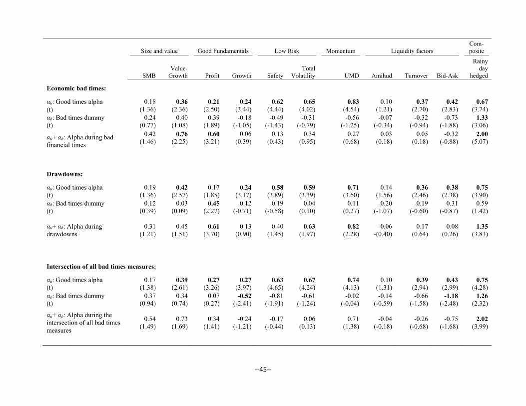
‐‐45‐‐  

Size and value Good Fundamentals Low Risk Momentum Liquidity factors

Com-posite

SMB Value-

Growth Profit Growth Safety Total

Volatility UMD Amihud Turnover Bid-Ask

Rainy day

hedged Economic bad times:

αu: Good times alpha 0.18 0.36 0.21 0.24 0.62 0.65 0.83 0.10 0.37 0.42 0.67(t) (1.36) (2.36) (2.50) (3.44) (4.44) (4.02) (4.54) (1.21) (2.70) (2.83) (3.74) αb: Bad times dummy 0.24 0.40 0.39 -0.18 -0.49 -0.31 -0.56 -0.07 -0.32 -0.73 1.33(t) (0.77) (1.08) (1.89) (-1.05) (-1.43) (-0.79) (-1.25) (-0.34) (-0.94) (-1.88) (3.06)

αu+ αb: Alpha during bad financial times

0.42 0.76 0.60 0.06 0.13 0.34 0.27 0.03 0.05 -0.32 2.00(1.46) (2.25) (3.21) (0.39) (0.43) (0.95) (0.68) (0.18) (0.18) (-0.88) (5.07)

Drawdowns:

αu: Good times alpha 0.19 0.42 0.17 0.24 0.58 0.59 0.71 0.14 0.36 0.38 0.75(t) (1.36) (2.57) (1.85) (3.17) (3.89) (3.39) (3.60) (1.56) (2.46) (2.38) (3.90) αb: Bad times dummy 0.12 0.03 0.45 -0.12 -0.19 0.04 0.11 -0.20 -0.19 -0.31 0.59 (t) (0.39) (0.09) (2.27) (-0.71) (-0.58) (0.10) (0.27) (-1.07) (-0.60) (-0.87) (1.42)

αu+ αb: Alpha during drawdowns

0.31 0.45 0.61 0.13 0.40 0.63 0.82 -0.06 0.17 0.08 1.35(1.21) (1.51) (3.70) (0.90) (1.45) (1.97) (2.28) -(0.40) (0.64) (0.26) (3.83)

Intersection of all bad times measures:

αu: Good times alpha 0.17 0.39 0.27 0.27 0.63 0.67 0.74 0.10 0.39 0.43 0.75(t) (1.38) (2.61) (3.26) (3.97) (4.65) (4.24) (4.13) (1.31) (2.94) (2.99) (4.28) αb: Bad times dummy 0.37 0.34 0.07 -0.52 -0.81 -0.61 -0.02 -0.14 -0.66 -1.18 1.26(t) (0.94) (0.74) (0.27) (-2.41) (-1.91) (-1.24) (-0.04) (-0.59) (-1.58) (-2.48) (2.32)

αu+ αb: Alpha during the intersection of all bad times measures

0.54 0.73 0.34 -0.24 -0.17 0.06 0.71 -0.04 -0.26 -0.75 2.02(1.49) (1.69) (1.41) (-1.21) (-0.44) (0.13) (1.38) (-0.18) (-0.68) (-1.68) (3.99)