Probabilistic Engineering Mechanics 22 (2007) 231–249www.elsevier.com/locate/probengmech

Rain-flow fatigue damage due to nonlinear combination of vectorGaussian loads

Sayan Guptaa,∗,1, Igor Rychlikb,2

a Department of Civil Engineering, Section of Hydraulic Engineering, Technical University of Delft, Stevinweg 1, PO BOX 5048, 2600 GA, Delft, The Netherlandsb Department for Mathematical Sciences, Chalmers University of Technology, SE-41296, Goteborg, Sweden

Received 18 October 2006; received in revised form 24 April 2007; accepted 25 April 2007Available online 10 May 2007

Abstract

The problem of estimating the mean rain-flow fatigue damage in randomly vibrating structures is considered. The excitations are assumedto be through a vector of mutually correlated, stationary Gaussian loadings. The load effect leading to fatigue damage is considered to be anonlinear function of the vector of excitation loads and is thus non-Gaussian. Its probabilistic characteristics are, however, unknown. The fatiguedamage is assumed to follow a linear damage accumulation rule. Though exact expressions for the mean fatigue damage are difficult to determine,approximations and bounds for the mean rain-flow fatigue damage can be developed. Computing these quantities requires the mean level crossingstatistics for the associated non-Gaussian response to be estimated. For the special case when the load effect can be expressed as quadraticcombinations of Gaussian processes, analytical expressions are developed for computing the level crossing statistics. These, in turn, are usedto determine approximations and the bounds for the mean fatigue damage. The applicability of the proposed method is demonstrated through anumerical example. With respect to this example, a comparative study on the quality of the bounds and the approximations is carried out viz–vizthe predictions from existing techniques available in the literature.c© 2007 Elsevier Ltd. All rights reserved.

Keywords: Expected fatigue damage; Rain-flow cycle counting; Non-Gaussian; Vector Gaussian process; Nonlinear combination

1. Introduction

Estimating the mean fatigue damage in structures subjectedto random loadings constitutes a key step in predicting theremaining lifetime of the structure. In randomly vibratinglarge engineering structures, the load effect that causes fatiguedamage at a particular location in the structure is usually dueto a large number of components. Often, the resulting loadeffect is obtained as a nonlinear combination of these individualcomponents and is thus non-Gaussian, even if the external loadsare Gaussian. For example, if the stress tensor does not varyuniaxially, then nonlinear functions of the stress tensor aresometimes used to define the stress metric and then rain-flow

∗ Corresponding author. Tel.: +31 15 27 88256; fax: +31 15 27 85 124.E-mail addresses: S.Gupta@tudelft.nl (S. Gupta), rychlik@chalmers.se

(I. Rychlik).1 Post-doctoral Researcher.2 Professor.

0266-8920/$ - see front matter c© 2007 Elsevier Ltd. All rights reserved.doi:10.1016/j.probengmech.2007.04.003

quantified to analyze the fatigue damage [25,26,34]. Anotherexample is when weakly nonlinear systems have to be used toanalyze responses to Gaussian loads. Here, the responses areoften approximated by means of quadratic transfer functions(Volterra quadratic input–output model), which also leads tostresses that are non-Gaussian but are a function of a vectorof Gaussian processes, viz.

Y (t) = g(X1(t), . . . , Xn(t)), (1)

where g(·) is a nonlinear deterministic function, X i (t)ni=1 are

stationary Gaussian processes and Y (t) is the non-Gaussianprocess that causes fatigue damage.

Computing the fatigue damage from a random time historytypically involves (a) splitting the time history into a number ofequivalent loading cycles corresponding to different amplitudelevels, (b) estimating the associated incremental fatigue damagefrom Wohler’s curves, and (c) applying a suitable damageaccumulation rule for computing the total fatigue damage.For a random load, the computed fatigue damage is a random

232 S. Gupta, I. Rychlik / Probabilistic Engineering Mechanics 22 (2007) 231–249

variable. In predicting the remaining lifetime of a structure,the mean fatigue damage is the metric that is generally used.Computation of the mean fatigue damage can be carried outeither in the time domain or in the frequency domain. Thetime domain approach involves repeated fatigue analysis onan ensemble of time histories having identical probabilisticcharacteristics. Subsequently, the mean fatigue damage iscalculated as the first moment. The accuracy of the estimatoris dependent on the sample size of the ensemble and is hence,time-consuming and computationally intensive. On the otherhand, frequency domain approaches provide fast and elegantmethods for estimating the mean fatigue damage. The latterapproach is especially useful during the design process, whena large number of analyzes may need to be carried out. Here,the focus is on developing analytical expressions that relate themean fatigue damage to the probabilistic characteristics, oftenin terms of the power spectral density function (PSD) and theprobability density function (pdf) of the loading process. Thepresent study belongs to this genre.

A key feature in fatigue estimation due to random loads liesin extracting and counting the equivalent load cycles from arandom time history [35]. A number of cycle counting methodshave been proposed in the literature, of which the peak countingmethod, range counting method, level crossing method andthe rain-flow cycle counting method are most widely used. Ofthese, the rain-flow cycle counting method [19] is consideredto lead to fatigue damage estimates that conform best withexperimental observations. In this study, we limit our attentionto developing approximations for the rain-flow fatigue damage.

The rain-flow cycle counting scheme, as proposed in [19],is highly nonlinear and difficult to model mathematically.To overcome this drawback, an equivalent but more suitabledefinition for mathematical derivations has been suggested [28].This has led to the development of approximations for theexpected rain-flow fatigue damage due to stationary, Gaussianloads [30] and for loads having Markov properties [29,10].An upper bound for the expected rain-flow damage wasgiven in [31]. The bound coincides with the narrow-bandapproximation for Gaussian loads proposed already in [3]. Forbroad-banded loads the method seriously overestimates thedamage. Questions related to estimating the fatigue damagefor broad-banded loadings and the accuracy when differentcounting methods are used have been addressed in [4,24,36,40].

While most studies in the literature have focused attentionon Gaussian loads, many of the realistic applications of fa-tigue damage involve non-Gaussian loadings. However, stud-ies on fatigue damage due to non-Gaussian loads are few andare of recent vintage. Semi-empirical expressions for predict-ing the rain-flow fatigue damage and its pdf have been de-veloped in [2,37]. Here, the parameters of the models weredetermined from regression analyzes on an ensemble of non-Gaussian time histories. Analytical approximations for themean fatigue damage for non-Gaussian loads obtained asmonotonic transformations of stationary Gaussian loads havebeen developed in [38,39]. The present authors, in an earlierstudy [34], developed analytical expressions which approxi-mate the rain-flow fatigue damage due to scalar non-Gaussian

Fig. 1. Definition of rain-flow cycle.

loads, obtained as non-monotonic transformations of stationary,Gaussian processes.

2. Problem statement

We consider the problem of estimating the expected rain-flow fatigue damage caused by non-Gaussian load processesthat can be expressed in the form as in Eq. (1). We assume thatthe fatigue damage due to Y (t) can be expressed through thewell known Palmgren–Miner’s hypothesis [23,20]. Here, theaccumulated linear fatigue damage caused by load Y (t), t ∈

[0, T ], is denoted by DT , and is given by DT =∑

αSbj , where

α and b are experimentally determined material properties,S denotes the stress levels for the counted cycles and thecounter j indicates the number of equivalent stress cyclescorresponding to an appropriate cycle-counting scheme. Here,we only consider the rain-flow fatigue damage that we denote asDT . Since Y (t) is a random process, DT is a random variable.The focus of this study is on developing approximations forE[DT ], where E[· ] is the expectation operator.

3. Expected rain-flow fatigue damage

We turn now to the computation of E[DT ], definedusing the rain-flow count and linear Palmgren–Miner damageaccumulation rule. For efficiency of presentation, we begin witha definition of the rain-flow fatigue damage.

3.1. Definition of rain-flow fatigue damage

Assume that x(t), t ∈ [0, T ] is a variable load functionhaving a finite number of local maxima. Assume that a localmaximum vi = x(ti ) in x(t) is paired with one particular localminimum uk , determined as follows:

• From the i-th local maximum (value vi ) one determines thelowest values in forward and backward directions between tiand the nearest points at which x(t) exceeds vi .

• The larger (less negative) of those two values, denoted byurfc

i , is the rain-flow minimum paired with vi , i.e., urfci is the

least drop before reaching the value vi again on either side.• Thus, the i-th rain-flow pair is (urfc

i , vi ); see Fig. 1.

Note that for some local maxima vi , the correspondingrain-flow minima urfc

i could lie outside the interval [0, T ]. Insuch situations, the incomplete rain-flow cycle constitutes theso called residual and has to be handled separately. In this

S. Gupta, I. Rychlik / Probabilistic Engineering Mechanics 22 (2007) 231–249 233

approach, we assume that the maximums in the residual, formcycles with the preceeding minimums in the residual.

The total damage DT defined using the rain-flow method andapplying the linear Palmgren–Miner damage accumulation ruleleads to

DT =

∑f (urfc

i , vi ) + Dres, (2)

where f (urfci , vi ) is the fatigue damage due to the rain-flow pair

(urfci , vi ) and Dres is the damage caused by cycles found in the

residual. In this study, we assume that f (urfci , vi ) is typically of

the form f (urfci , vi ) = α(vi −urfc

i )b, where α > 0 and b > 1 areexperimentally defined material parameters. It must be notedthat f (·, ·) is at least twice differentiable.

An alternative definition for the rain-flow damage in Eq. (2)has been presented in [32]. Here, for a smooth load, x(t), therain-flow damage is given by

DT = −

∫+∞

−∞

∫ v

−∞

f12(u, v)N (u, v)dudv

+

∫+∞

−∞

f2(u, u)N (u)du, (3)

where f2(u, v) =∂ f (u,v)

∂ vand f12(u, v) =

∂2 f (u,v)∂ u∂ v

. Here, for asmooth loading function x(t),

• N (u) is the number of up-crossings of level u by x(t),t ∈ [0, T ], i.e. the number of solutions to equation x(t) = u,such that, x(t) > 0.

• N (u, v) is the number of up-crossings of an interval [u, v] byx(t), i.e. the number of solutions to equation system x(t) =

u, x(s) = v, 0 ≤ t < s ≤ T , such that, x(t) > 0, x(s) > 0and for all z, t < z < s, u < x(z) < v. (Note thatN (u, u) = N (u)).

Here, x(t) denotes a derivative of x(t) with respect to time t .Let (ui , vi ) be a sequence of cycles found in the load x(t) (bothrain-flow cycles and the one found in the residual). It can thenbe shown that, N (u, v) is equal to the number of pairs (ui , vi ),such that vi > v and ui < u [32]. This is the basis for Eq. (3).

It must be noted that if f (u, v) = (v −u), following Eq. (3),we obtain

DT =

∫+∞

−∞

N (u)du (4)

as the first integral becomes equal to zero. If f (u, v) = (v−u)2,Eq. (3) leads to DT = 2

∫+∞

−∞

∫ v

−∞N (u, v)dudv. Moreover,

for f (u, v) = (v − u)α , where α ≥ 2, the second integral inEq. (3) is always identically equal to zero.

In the following, for simplicity of presentation, we assumethat the function f (·), defined in Eq. (2), is such that f2(v, v) =

0, for all v.The rain-flow cycles measure the sizes of closed hysteresis

loops, while the residual represents the memory of the materialto previously experienced loads. The sizes and number of localextrema that constitute the residual will depend on the timewhen the structure was first loaded. Suppose that it happenedat time T0 ≤ 0. Then the damage DT , accumulated in the

interval [0, T ], will also depend on T0. More precisely, it willbe given by Eq. (3) with N (u, v) defined as follows: N (u, v) isthe number of solutions to equation system x(t) = u, x(s) = v,0 ≤ s ≤ T and T0 ≤ t < s, such that, x(t) > 0, x(s) > 0and for all z, t < z < s, u < x(z) < v. Clearly, the damage isa decreasing function of T0. Note that the process of damageaccumulation cannot be stationary since it is an increasingprocess. However, if T0 = −∞, it has stationary increments.On the other hand, if T0 is not infinite, then the increments areonly approximately stationary for large T .

3.2. Random loads — expected damage increase

For a random load X (t), 0 ≤ t ≤ T , the number ofinterval crossings, N (u, v) is a random variable. Consequently,the rain-flow fatigue damage, at a particular time instant, is alsoa random variable. Determining the probabilistic characteristicsof this variable is not easy. On the other hand, estimating themean of the rain-flow fatigue damage is comparatively easierand is generally used to predict the expected life of the structurein question. As mentioned before, the damage depends on thetime T0 ≤ 0 when the load started to act on the structure. Hence,in order to study the stationary damage increase in the period oflength T , we assume that T0 = −∞.

If the joint pdf for cycle tops (v) and bottom (u) is known,then the expected damage can be computed as

E[DT ] = T ν

∫∫f (u, v)prfc(u, v)dudv, (5)

where prfc(u, v) is the joint pdf of urfc (minima) and v

(maxima) of a rain-flow cycle. Note that the rain-flow matrixis the discretized pdf, prfc(u, v), which is then normalized sothat elements in the matrix sums to one. The numerical value ofexpected damage, E[DT ], is obtained by

(a) multiplying (element-wise) matrix with cycles damagesf (·) and the rain-flow matrix prfc,

(b) subsequently, summing all the elements in the resultantmatrix f · prfc, and

(c) finally, multiplying by the expected number of cycles T ν.

Here, ν is the intensity of cycles, i.e. the expected number ofcycles in unit time.

Alternatively, using Eq. (3) and by changing the order ofintegrations (Fubini’s theorem), we obtain

E[DT ] =

∫+∞

−∞

∫ v

−∞

f12(u, v)E[N (u, v)]dudv. (6)

Since for stationary processes, the expected number ofintervals up-crossings are proportional to time duration T , theproportionality constant µ(u, v) can be termed as the intensityof interval up-crossings and is equal to E[N (u, v)] for T = 1and T0 = −∞. The expected damage increase in period T canbe shown to be proportional to the loading time duration T , andis written as

E[DT ] = T∫

+∞

−∞

∫ v

−∞

f12(u, v)µ(u, v)dudv. (7)

234 S. Gupta, I. Rychlik / Probabilistic Engineering Mechanics 22 (2007) 231–249

Consequently, we can write

d =

∫+∞

−∞

∫ v

−∞

f12(u, v)µ(u, v)dudv, (8)

where d can be called the damage intensity — the expectedgrowth of the damage in unit time. The primary difficultyhere is that, in general, there are only a few cases where theintensity µ(u, v) or the pdf prfc(u, v) can be computed exactly.The explicit results are available when loads possess a Markovproperty or have very simple structure.

3.3. Bound for the expected damage

In situations where explicit evaluation of µ(u, v) orprfc(u, v) is not possible, one can evaluate bounds for theintensity crossings. Thus, if µ(u) be the up-crossing intensityof level u by X (t), i.e. E[N (u)] = T µ(u), then one can showthat

µ(u, v) ≤ min[µ(u, u), µ(v, v)] = µ(u, v), (9)

where µ(u, u) = µ(u). The proof is given in [31]. Note thatµ(u, v) ≤ µ(u) follows from the fact that for symmetrical loadsthe expected number of up-crossings of interval [u, v] that endin [0, T ] is equal to the expected number of down-crossingsof the interval [u, v] that end in [0, T ]. Since the intensity ofdown-crossings of level u is equal to µ(u), the bound follows.Consequently, one can write

E[DT ] ≤ T∫

∞

−∞

∫ v

−∞

f12(u, v)µ(u, v)dudv = T · d+. (10)

The applicability of Eq. (10) lies in the ease of computationof the mean up-crossing rate, µ(u). This can be computed usingRice’s formula [27], given by

µ(u) =

∫∞

0x pX X (u, x)dx, (11)

where pX X (x, x) is the joint pdf of the process, X (t), and itsinstantaneous time derivative, X(t). Clearly, µ(u) combinedwith Eq. (9) gives a conservative estimate of the expecteddamage.

3.3.1. The narrow-band approximationIn the early 1960s, the narrow-band approximation was

presented by Bendat [3] at a time when a definition for rain-flowcycle counting was not yet available. Bendat proposed that for astress time history, S(t), the cycle amplitude has the followingprobability distribution:

P(S ≤ u) = 1 −µ(u)

µ(0). (12)

He also proposed to approximate the intensity of cycles bymeans of the zero-crossing intensity, µ(0). It can be easilyshown that the expected damage increase, estimated usingBendat’s approach, coincides with the bound in Eq. (9) for thecase of symmetric loads, such that, µ(−u) = µ(u).

3.4. Asymptotic correction of the interval crossing intensity

The bounds for the expected damage, computed using theabove arguments, may be extremely conservative when loadsbecome broad-banded. In order to make the estimated damageless conservative, we focus on approximating µ(u, v) usingasymptotic properties of level crossings.

For large values of the material parameter b, it is obvious thatthe contribution to the damage is mostly from the large cycles.Mathematically, this damage is given by the integral

−

∫ u0

−∞

∫+∞

v0

f12(u, v)µ(u, v)dudv

≤ −

∫ u0

−∞

∫+∞

v0

f12(u, v) min[µ(u), µ(v)]dudv. (13)

Now using the results derived in [15,16], one knows thatasymptotically, i.e. when u0 tends to minus infinity whilev0 goes to plus infinity, the up-crossings of levels u and v

form independent Poisson processes with intensities µ(u) andµ(v), respectively. Using this property, one can asymptoticallyapproximate

µ(u, v) ≈µ(u)µ(v)

µ(u) + µ(v). (14)

Hence

−

∫ u0

−∞

∫+∞

v0

f12(u, v)µ(u, v)dudv

≈

∫ u0

−∞

∫+∞

v0

f12(u, v)µ(u)µ(v)

µ(u) + µ(v)dudv. (15)

The formula (14) was first given in [13].Let now µ(u, v) = µ(u)µ(v)/µ(u)+µ(v), for u < u0 and

v > v0 and µ(u, v) = µ(u, v), otherwise. Then, one obtains

dpoiss=

∫∞

−∞

∫ v

−∞

f12(u, v)µ(u, v)dudv, (16)

where dpoiss denotes the asymptotically corrected (approximatebound) for the damage intensity. Note that dpoiss < d+.

3.5. The transformed Gaussian approximation

An alternative approach to approximating the intervalcrossing rate is to use the so-called transformed Gaussianprocess. Here, one approximates the random (true) load Y (t) byY (t) = G(X (t)), where G(·) is a non-decreasing deterministicfunction and X (t) is a stationary, Gaussian process. Theexpected damage intensity in Y (t) can subsequently beestimated using the so-called Markov chain of turning points.The method is well described in the literature; see, e.g. [29,14,5,30,10,12,17]. The software to compute the approximationis available in WAFO; see [8]. In this approach, one needs tospecify both the transformation G(·) and the spectral densityS(ω) of X (t).

The problem of selecting the transformation G(·) has beenaddressed in the literature. Usually, it is proposed to select G(·),

S. Gupta, I. Rychlik / Probabilistic Engineering Mechanics 22 (2007) 231–249 235

such that the pdf of Y (t) and Y (t) coincide; see [38,39]. In [33],it was proposed to choose G(·) such that, the processes Y (t)and Y (t), have the same upcrossing intensity (up to a factor).A consequence of such transformations is that the boundcoincides for both the loads, Y (t) and Y (t), and in the specialcase when b = 1, the corresponding expected rain-flow fatiguedamages are identical. In the same paper, it was also discussedhow to estimate both the transformation and the spectrumfrom the measured signal. For the quadratic type of responsesstudied in this paper, X (t) can be assumed to be the linear(Gaussian) approximation of the response. The correspondingPSD, S(ω) can subsequently be easily determined. When thespectrum S(ω) and the transformation G(·) have been selected,the process Y (t) is fully specified.

The use of transformed Gaussian processes is, however,not always recommended. For processes with large cycles thatoccur in clusters, e.g. due to potholes in roads [6] or when theload consists of a slowly varying process with superimposedhigh-frequency components, other methods need to be used;see [33]. However, for quadratic loads, the use of a transformedGaussian approach can be quite useful.

4. The second-order responses

We now focus on deriving expressions for the responseof randomly vibrating structures. The general form of thegoverning equations of motion, when discretized using finiteelements, can be written as

MY(t) + CY(t) + KY(t) = F(t). (17)

Here, M, C and K are the structure mass, damping and linearstiffness matrices of dimensions n ×n, Y(t), Y(t) and Y(t) are,respectively, the vectors of nodal accelerations, velocities anddisplacements and F(t) is the vector for nodal forces, of sizen × 1. Let the focus of our attention be the structure responseat a particular location of the structure and denoted by Y (t).We assume that the external excitations can be modeled asstationary Gaussian processes X j (t)n

j=1 and that the forcevector F(t) is obtained as a nonlinear function of the externalexcitations X j (t)n

j=1. This, in turn, means that the structureresponse can be expressed, at least in principle, as in Eq. (1).

Studying the increase in the expected rain-flow damagefor quadratic responses is a very difficult problem. Oneobvious possible approach would be to simulate the loads andto compute the corresponding damage due to the response.However, in this approach, one needs to simulate an ensembleof long sequences of the response to obtain reliable estimatesof the damage; see the numerical example discussed later inthis paper. This can be quite time-consuming and expensive,especially at the design stage, which includes repetitiveiterations. Thus, there is a need to develop alternative methodsthat can lead to approximate estimates of the damage in afast and reliable manner. In this paper, we give a generalrepresentation (see Eq. (32)), for which most quadratic responseproblems can be written down. As has been already discussed,the crux of the problem lies in computing the mean crossingintensities for such processes. For computing the crossing

intensity for loads which are represented in the form ofEq. (32), we consider two approaches — the first one is basedon the integration of Rice’s formula Eq. (11) using the MonteCarlo method [11], and the second, is the so-called SORMasymptotic method, proposed first in [7]. Brief discussions ofthese methods are presented in the appendices of this paper.The computed crossing intensity, µ(u), is subsequently used toassess the expected damage as discussed in the previous section.

4.1. Definition of the g function in Eq. (1)

We now consider the special class of problems where theexcitation load, F(t), has a linear component, FL(t), anda quadratic component, FQ(t). Since Eq. (17) is linear, theresponse can be expressed as a sum Y (t) = YL(t) + YQ(t),where YL(t) is the zero-mean Gaussian response when onlyFL(t) acts on the structure and YQ(t) is the quadratic correctionfor nonlinearity due to the presence of load FQ(t).

Let us assume that FL(t) and FQ(t) are linear and quadraticfunctions of a zero-mean stationary, Gaussian random process,ζ(t), with a specified one-sided PSD, Sζ (ω). We define theGaussian load ζ(t), in the limit as N tends to infinity, to beof the form

ζN (t) =

N∑j=−N

σ j

2(U j − iV j )eiω j t , (18)

where U j , V j , j > 0, are independent standard normalvariables and U− j = U j , V− j = −V j , ω− j = −ω j . Moreover,ω j = jωc/N and σ 2

j = Sζ (ω j )∆ω, where j = 1, . . . , N ,σ0 = 0, ∆ω = ωc/N , ω is the frequency defined in 0 ≤ ω ≤ ωcand ωc is the cut-off frequency, such that, Sζ (ω) = 0, ifω > ωc. For the sake of simplicity in representation, we writeζ(t) instead of ζN (t). Thus, in the discretized form, the linearresponse, YL(t), is given by

YL(t) =

N∑j=−N

σ j

2H1(ω j )(U j − iV j )eiω j t , (19)

and the quadratic response, YQ(t), is given by

YQ(t) =

N∑j=−N

N∑k=−N

σ j

2σk

2H2(ω j , −ωk)

× (U j − iV j )(Uk + iVk)ei(ω j −ωk )t . (20)

Here, H1(ω) and H2(ω1, ω2) are the linear and the quadratictransfer functions for the structural response at the desiredlocation.

Using standard techniques (see [1,18]), it is possible toexpress the response Y (t) in terms of 2N independent, zero-mean, unit variance processes, Zi (t)2N

i=1 in the form

Y (t) = g(Z(t)) =

[R(q)

=(q)

]′

Z(t) +12

Z(t)′AZ(t), (21)

where q is the column vector containing [σ j H1(ω j )]. Here,Cov[Z(0), Z(0)] = I, where I is the identity matrix of size

236 S. Gupta, I. Rychlik / Probabilistic Engineering Mechanics 22 (2007) 231–249

2N × 2N . The auto- and cross-covariance between Z(t) andits time derivative Z(t) are given by

Cov[Z(0), Z(0)] =

[0 −WW 0,

](22)

Cov[Z(0), Z(0)] =

[W2 00 W2

], (23)

where 0 is a 2N × 2N matrix with all elements being zeros.Computation of the mean up-crossing rate of Y (t) can becarried out using the algorithms presented in the appendices.

4.2. The standard representation of the quadratic responses

The limitation of using Eq. (21) is that for accuraterepresentation, the number of discretized frequencies, N shouldbe large, which, in turn, introduces a large number of randomvariables into the formulation. This, in turn, requires largercomputational effort while calculating the mean up-crossingrate, µY (u). We next focus on an approach which allows a largenumber of frequencies to be used but still keeps N relativelylow.

Since the matrix A of size 2N ×2N is real and symmetrical,it can be diagonalized. Let P be the matrix containing the ortho-normal eigenvectors of A and let Λ be the diagonal matrix witheigenvalues λ j of A on the diagonal, such that,

A = PΛP′. (24)

Sorting the eigenvectors in such a way, so that |λ1| ≥ |λ2| ≥

· · · |λ2N |, then YQ(t) can be represented as

YQ(t) =12P′Z(t)′ΛP′Z(t) =

12

2N∑j=1

λ j X2j (t), (25)

where X′(t) = [X1(t), . . . , X2N (t)] = Z(t)′P are zero-mean,stationary Gaussian processes. In addition, since Z(t) = PX(t),YL(t) can be expressed as

YL(t) =

[R(q)

=(q)

]′

PX(t) = [γ1, . . . , γ2N ]X(t). (26)

Now the response Y (t) can be written as

Y (t) = g(PX(t)) = g(X(t))

=

2N∑j=1

γ j X j (t) +12

2N∑j=1

λ j X2j (t), (27)

which is a function of 2N stationary Gaussian processes X(t).Clearly, the expression in Eq. (27) is simpler than in Eq. (21).The corresponding covariance matrices for X(t) and itstime derivative are more complicated and are given byCov[X(0), X(0)] = I and

Cov[X(0), X(0)] = PT[

0 −WW 0

]P, (28)

Cov[X(0), X(0)] = PT[

W2 00 W2

]P, (29)

which are usually not diagonal matrices. However, theadvantage of using Eq. (27) is that when the absolute valuesof coefficients |λm |, m > k are close to zero, the associatedterms can be omitted. This leads to the following truncatedrepresentation of Y (t), given by

Y app(t) =

k+1∑j=1

γ j X j (t) +12

k+1∑j=1

λ j X j2(t), (30)

where k ≤ 2N , λk+1 = 0, γk+1 =

√∑2Nj=k+1 γ 2

j and X j (t) =

X j (t) for j ≤ k and Xk+1(t) =∑N

j=k+1 γ j/γk+1 X j (t). Thus,Xk+1(t) is a zero-mean Gaussian process with variance equalto∑2N

j=k+1 γ 2j /γ 2

k+1. The index k can be chosen using thefollowing method. First, note that Var[Y (t)] − Var[Y app(t)] =

2∑2N

j=k+1 λ2j . Next, k is chosen so that the variance of Y app(t)

differs by less than ε% from the exact, i.e.

Var[Y (t)] − Var[Y app(t)] ≤ε

100Var[Y (t)]. (31)

In this case also, we can use the algorithms discussed in theappendices, for computing the mean up-crossing rate µY (u).However, certain modifications may be carried out which canlead to simplification in the application of the method. Thisrequires rewriting the response Y (t), as

Y (t) =

k∑i=1

Γi X i (t) + Λi X2i (t) + Γk+1 Xk+1(t)

= YN G(t) + YG(t). (32)

Clearly the process Y app(t) is of the form of Eq. (32). It is alsoobvious that YN G(t) is a non-Gaussian process and YG(t) isa Gaussian process. Appendix B details a different approachfor computing the mean up-crossing rate, which simplifies thecomputations presented in Appendix A.

Finally, it must be noted that a Gaussian approximation forY (t) can be obtained by letting all Λi = 0 in Eq. (32). Themotivation for considering this approximation lies in the factthat dealing with Gaussian processes is much simpler and thequality of this approximation vis–vis dealing with processes ofthe form of Eq. (32) needs to be investigated. Thus, we considerthe following Gaussian approximation YL(t), given by

YL(t) =

k+1∑i=1

Γi X i (t). (33)

In the remaining sections of this paper, the transformedGaussian approximation for Y (t) will be approximatedby G(YL(t)). Here, the transformation G(·) ensures thatthe processes YL(t) and Y (t) have identical crossingcharacteristics.

5. Numerical example and discussion

The theory proposed in this paper is illustrated througha numerical example. The example considers the rain-flowfatigue damage at the support of a cantilever beam, subjectedto randomly varying wind loads. The wind loads are modeled

S. Gupta, I. Rychlik / Probabilistic Engineering Mechanics 22 (2007) 231–249 237

Fig. 2. Schematic diagram of the 10-dof cantilever beam subjected to randomwind excitations.

as stationary Gaussian processes. The forces imparted on thebeam are obtained as quadratic functions of the wind loads.Consequently, the theory proposed in this paper has been usedfor assessing the mean fatigue damage. The predictions havebeen compared with those obtained from full-scale Monte Carlosimulations. This involves digital generation of an ensemble oftime histories for the response quantities of interest, from theavailable PSD functions. Corresponding to each sample timehistory, a deterministic analysis is carried out using the WAFOtoolbox [8] to compute the associated rain-flow fatigue damage.The expected fatigue damage is subsequently computed as thefirst moment of the computed fatigue damages.

The wind velocity is modeled as a stationary Gaussianprocess with specified mean wind speed, ζm , and PSD,Sζ (ω). The force due to wind loadings is given by F(t) =

1/2Cdρlb(ζ(t) + ζm)2, where ζ(t) is a zero-mean Gaussianrandom process denoting the wind velocity at the tip of thebeam, Cd is the drag coefficient, ρ is the air density and l andb are the dimensions of the structure. The beam is modeled asa simple lumped-mass model of 10-dof. The variation of thewind velocity along the beam span is taken to be deterministicand is assumed to be parabolic; see Fig. 2. The normalizedconstants, χi

10i=1, are used to denote the wind velocity profile

and are such that the maximum velocity is at the beam tip. TheDavenport spectrum is assumed for Sζ (ω), and is given by

Sζ (ω) = κζ 2

f

nx2

(1 + x2)4/3 , (34)

where x = (L ref/z)(ωz/ζ10) = (1200/z) f , f = nz/ζz is thenormalized frequency, n = ω/(2π) is the frequency in Hz,Sζ (n) is the PSD of ζ(t) in m2 s−2 Hz−1, z is the distance fromthe fixed end in m, ζz is the mean wind speed in m/s measuredat distance z from the support, κ is the surface drag coefficient,ζ f is the friction velocity in m/s and L ref is the representativescale length. Denoting η = 0.5Cdρlb = 0.0250, the wind forceF(t) can be expressed in terms of two dynamic componentsFl(t) = 2ηζmζ(t) and Fq(t) = ηζ(t)2. The contribution fromthe mean wind velocity, ηζ 2

m , acts as a constant load and has nobearing on the dynamic response of the structure.

The dynamic analysis is carried out by modeling the beam asa simple 10-dof lumped-mass model. The governing equationsof motion are as in Eq. (17), with F(t) = Υ(Fl(t) + Fq(t)).Here, Υ is the influence matrix of size 10 × 1, and since the

spatial variation of the wind is assumed to be deterministic, theelements of Υ are constants denoted as χi , (i = 1, . . . , 10).If the spatial variation of wind is assumed to be stochastic,the wind velocities acting along the length of the buildingconstitute a vector of mutually correlated Gaussian processes.This implies that the problem can be viewed as a multipleexcitation problem. The corresponding formulation has beendetailed in Appendix C. However, as has been shown, apartfrom increasing the complexity of the computations, this doesnot place any restrictions on the proposed methodology. If thewind effects are not turbulent, it is expected that the windvelocities along the profile bear a strong correlation and theerrors induced in the calculations by considering the windvariation to be deterministic, are expected to be small. Theerror can, however, be quite significant if the wind is turbulentand the wind velocities acting at the different nodes are weaklycorrelated. However, as the purpose of this numerical exampleis to illustrate the proposed methodology, for the sake of easeof illustration, we do not take into account the effect of spatialrandom inhomogeneities of the wind velocities.

The damping is assumed to be proportional, such that C =

η1M + η2K, where η1 and η2 are the mass and stiffnessproportionality constants. An eigenvalue analysis reveals thatthe first five natural frequencies of the structure are 2.32,6.90, 11.32, 15.49 and 19.32 rad/s, respectively. Assuming thatdamping is 10% in the first two modes, we obtain η1 = 0.3467and η2 = 0.0217.

The maximum stresses are developed at the base of thecantilever beam and the rain-flow fatigue damage is calculatedfor this location. ζ(t) is modeled as a Gaussian process and isexpressed using the approximation in Eq. (18). Since structurebehavior is assumed to be linear (see Eq. (17)), the responseprocess can be expressed as a sum Y (t) = YL(t)+YQ(t), whereYL(t) is the Gaussian response when only FL(t) acts on thestructure and YQ(t) is the quadratic correction for nonlinearitydue to the presence of load FQ(t). This enables rewriting theresponse Y (t) as in Eq. (21) and as in Eq. (27). Here, the linearand quadratic transfer functions are obtained as

H1(ω) = [−ω2M + iωC + K]−1Υ (35)

H2(ω1, ω2) = H1(ω1 + ω2). (36)

In this example, we discretized the PSD, Sζ (ω), into 200segments, i.e. N = 200. Thus, the response Y (t), is obtained asa nonlinear combination of a 400D vector of random processesX(t). Fig. 3 illustrates the PSD of YL(t). Fig. 4 illustrates asample time history of stress, Y (t), developed at the root of thebeam, calculated using Eqs. (21) and (27). This illustrates thatboth these representations are equivalent.

5.1. Number of quadratic terms in Eq. (30) and accuracy ofestimates of µY (u)

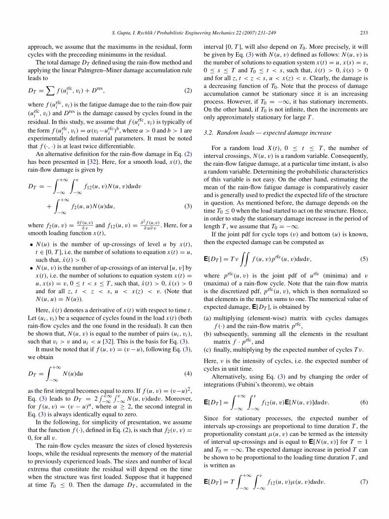
We next focus on fixing k in Eq. (30). Fig. 5 illustrates thevariation of k with respect to ε. We consider ε = 0.3 andcorrespondingly, k turns out to be equal to 9. The response cannow be approximated by Y app(t) as in Eq. (30), containing 10

238 S. Gupta, I. Rychlik / Probabilistic Engineering Mechanics 22 (2007) 231–249

Fig. 3. Power spectral density function for YL (t).

Fig. 4. Sample time history of response Y (t).

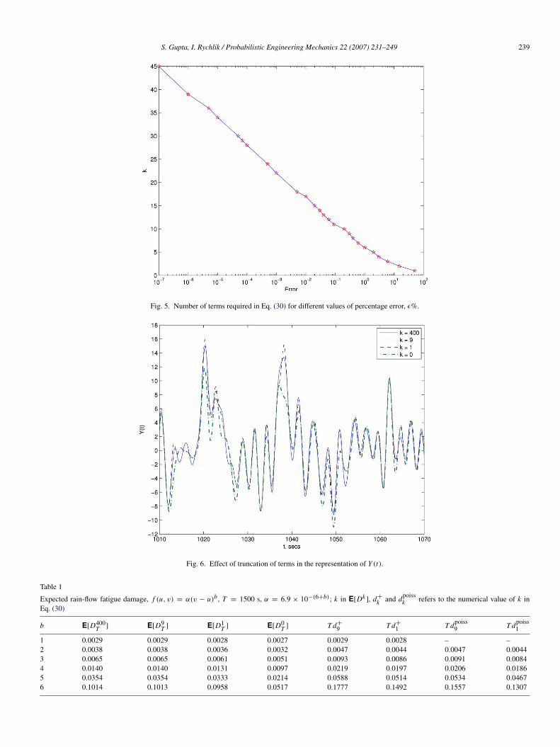
terms. Fig. 6 compares a sample response time history Y app(t)with k = 9 and with Y (t) (when there are no truncationsi.e. k = 400). A very good agreement between the tworepresentations is observed. The accuracy of this representationin estimating µY (u), can be verified from Fig. 7. Here, wepresent a comparison between the estimated upcrossing ratesfor Y (t), when Monte Carlo simulations are used on anensemble of 100 time histories consisting of k = 400 and whenk = 9. The corresponding comparison of the predicted levelcrossing rates between the integration method (Appendix A)

and the SORM approach (Appendix D) is shown in Fig. 8 in thelog-scale.

We next explore the possibility of further truncation ofquadratic terms in Eq. (30). We consider the case where k = 1.Here, there is only one quadratic term in Eq. (30) and thiscorresponds to ε = 50. For this example, the representation isstill quite good; see Fig. 6. However, Fig. 9 reveals that there aredifferences in the identified rain-flow cycles. Table 1 presentsa comparison of the expected rain-flow fatigue damages forthe cases k = 400, k = 9 and k = 1 for various

S. Gupta, I. Rychlik / Probabilistic Engineering Mechanics 22 (2007) 231–249 239

Fig. 5. Number of terms required in Eq. (30) for different values of percentage error, ε%.

Fig. 6. Effect of truncation of terms in the representation of Y (t).

Table 1

Expected rain-flow fatigue damage, f (u, v) = α(v − u)b , T = 1500 s, α = 6.9 × 10−(6+b); k in E[Dk], d+

k and dpoissk refers to the numerical value of k in

Eq. (30)

b E[D400T ] E[D9

T ] E[D1T ] E[D0

T ] T d+

9 T d+

1 T dpoiss9 T dpoiss

1

1 0.0029 0.0029 0.0028 0.0027 0.0029 0.0028 – –2 0.0038 0.0038 0.0036 0.0032 0.0047 0.0044 0.0047 0.00443 0.0065 0.0065 0.0061 0.0051 0.0093 0.0086 0.0091 0.00844 0.0140 0.0140 0.0131 0.0097 0.0219 0.0197 0.0206 0.01865 0.0354 0.0354 0.0333 0.0214 0.0588 0.0514 0.0534 0.04676 0.1014 0.1013 0.0958 0.0517 0.1777 0.1492 0.1557 0.1307

240 S. Gupta, I. Rychlik / Probabilistic Engineering Mechanics 22 (2007) 231–249

Fig. 7. Estimated up-crossing rates, µY (u), using different methods, when k = 9 in Eq. (30).

Fig. 8. Comparison of estimated µY (u) between the Integration method and Asymptotic method.

levels of α = 6.9 × 10−(6+b) and b. Fig. 10 compares thepredicted µY (u) for the case when k = 1, as obtained byMonte Carlo simulations as well as when they are computedusing the theory presented in Appendix A. It can be observedthat for negative threshold levels, the upcrossing rates areunderestimated, when Eq. (30) contains only one quadraticterm. However, the predicted upcrossing rates using MonteCarlo simulations and the theory presented in Appendix Aare in good agreement (though erroneous), for all thresholdlevels. This indicates the robustness of the theory presented

in Appendix A. The differences with the benchmark can beattributed to the truncation of too many terms resulting in about50% of the quadratic variability being lost.

We next explore the possibility of doing away with quadraticterms altogether by taking k = 0. Thus, Eq. (30) contains onlylinear terms and Y (t) = YL(t), is a Gaussian random process.Fig. 4 compares the corresponding sample time history with thecase when k = 400. We observe that some cycles are missedand the amplitudes of the rain-flow cycles are underestimated(see also Fig. 9). The estimated µY (u) significantly differs from

S. Gupta, I. Rychlik / Probabilistic Engineering Mechanics 22 (2007) 231–249 241

Fig. 9. Rain-flow cycles for sample Y (t).

the benchmark values-underestimated for most threshold values(see Figs. 7 and 10). The computed rain-flow fatigue damages,tabulated in Table 1, clearly show that the predictions aresignificantly different if k = 0. This highlights the importanceof taking into account the non-Gaussian features of the structureresponse.

It must be noted that by truncating from 400 to 9 quadraticterms, substantial reduction in computational effort is achievedwithout introducing any significant truncation error. On theother hand, further reduction to just one quadratic term doesnot provide any significant gain in terms of computational costsbut introduces discretization errors. Clearly, the truncation to 9quadratic and one Gaussian component perfectly describes thevariability of the stresses at the location where the damage dueto fatigue is of interest. One could ask the question whetherthere would be a difference if one wished to compute the oneyear value of the load, i.e., the level u which has upcrossingintensity 3.2 × 10−8. This is equivalent to one crossing of thelevel u in T = 3600 × 24 × 365 s. Thus, the one year levels arecomputed to be 54.82, 54.80 and 54.78 for the cases when k =

1, k = 9 and k = 20 respectively. The result that asymptoticallyonly one quadratic term is needed is not surprising. As has beendiscussed in Appendix D, for quadratic loads the term withhighest coefficient λ determines the asymptotic properties. Itmay be noted here, that for the case of extreme responses, theMonte Carlo integration of Rice’s formula may not always be anappropriate method, especially if k is large. This is because thesize of the vector of random variables that need to be simulatedfor the Monte Carlo integration may be prohibitively large.On the other hand, the asymptotic SORM method gives veryaccurate results at a much less computational cost. It can thusbe concluded that the process Y (t) with 9 quadratic terms canbe used to describe the response and will be solely used in thefollowing.

6. Estimates of damage intensity d

In this section, the bounds d+ for the damage intensityare presented. These bounds, which have been defined in Eq.(10), are based on crossing intensities µ(u), which in turn, arecomputed using the algorithms presented in the appendices.The bounds are compared with the estimated damage intensitiesfrom simulated samples of the response Y (t) and with theapproximate bound, dpoiss, computed by means of Eq. (16).

Additionally, the method of transformed Gaussian processis used to approximate the response and compute the damageintensity in the process. The process is defined as follows.

Let Y (t) = G(YL(t)), where

G(u) =

√−2Var(YL(0)) ln(µa(u)/µa(0)) if u > 0,

−√

−2Var(YL(0)) ln(µa(u)/µa(0)) if u < 0.(37)

Here, µa(u) is the SORM approximation of the crossingintensity of the response process Y (t), computed using thealgorithm presented in Appendix D.

The process Y (t) crosses the level u with intensity µa(u).This is different from the crossing intensity of the responseµ(u) for low u-levels. Since the two crossing intensitiesdiffer only for small u-levels, the difference is small (lessthan 5%) when checked by Monte Carlo simulations. Thisdifference is smaller than discretization errors and is negligiblein comparison with other sources of uncertainty.

This discrepancy in the computation of crossing intensitiesfor low u-levels is more than offset by the gain in the simplicityof the approach, which is a consequence of the fact that thezero upcrossing intensity of YL(t) process is equal to µa(0);see Appendix D. If it is required that Y (t) be transformed toYL(t) and has the mean level crossing rate equal to µ(u), thentime also needs to be scaled, i.e. Y (t) = g(YL(c · t)) for someconstant c.

The spectrum of YL(t) is given in Fig. 3, whilethe transformation G(·) is shown in Fig. 11. However,before presenting the results, we make some comments onuncertainties while estimating the damage intensities.

6.1. Uncertainties in estimation of damage intensity

When evaluating the quality of an approximation, one isoften comparing the computed damage intensity d for thedamage functions f (u, v) = (v − u)b, b taking values in asuitable interval. The damage intensity can be estimated froman observed (or simulated) load and can be compared againstthe derived approximation. We comment on three aspects ofsuch comparisons.

Bias: As we have already discussed, due to the length T ofthe signal used to estimate the damage intensity, the observeddamage is smaller (on average) than the expected damageincrement. This bias is due to the fact that the load is unknownbefore one starts to measure the signal, i.e. T0 = 0, while in thedefinition of d one assumes that the loads have been acting fora long time prior to measurements.

Variability of the damage: Clearly, new measurements of thesignal will give different estimates of the damage intensity d.

242 S. Gupta, I. Rychlik / Probabilistic Engineering Mechanics 22 (2007) 231–249

Fig. 10. Estimated up-crossing rates, µY (u), using different methods, when k = 1.

In practice, one has only one estimate of d and hence, it isof interest to estimate how large is the statistical uncertainty,due to the finite length of observation interval T . Since we arecomparing damage intensities d for different fatigue exponentsb, it is more convenient to analyze the logarithms of theestimated damages. In Fig. 12, we present a normal probabilityplot for base 10 logarithms of the observed damage intensities(computed using Eq. (38)), when b = 6 for two cases: (a)for time T = 1500 s (when the signal consists of about 500cycles) and (b) T = 3000 s (which corresponds to a signalwith about 1000 cycles), for an ensemble of 100 simulatedsignals of the response Y (t). The dots to the right correspondto the logarithms of damages for longer signals. We observethat the medians differ owing to the bias (T0 = 0) by 0.06, i.e.15%. Furthermore, the variance of the logarithms of d estimatesslightly decreased from 0.2 to 0.18, for b = 6. We can thereforeconclude that the statistical variability measured by standarddeviation is much larger than the bias.

Discretization errors: There are primarily two types ofdiscretization error. One possible source of discretization erroris when one uses the following property of stationary andergodic loads, viz. the damage intensity d = E[DT ]/T =

limT →∞ DT /T , and hence

d ≈DT

T. (38)

However, often in field experiments, the real loads are savedin the form of a rain-flow matrix prfc(u, v). Subsequently, thedamage intensity is computed using Eq. (5), viz.

d ≈ ν

∫∫f (u, v)prfc(u, v)dudv. (39)

Computations of rain-flow matrices implies that the rain-flow cycles are discretized and this is the second source of

Fig. 11. The function G(·) for the transformed Gaussian approximation.

discretization errors. Hence, the two approaches Eqs. (38) and(39) may give different estimates for the damage intensity.There can be considerable differences for f (u, v) = (v − u)b,when b is large. Consequently, if two methods have to becompared, one should use the same method for computing thedamage, i.e. by means of a direct sum or the rain-flow matrix.

6.1.1. Example of discretization errorWe consider 100 simulated responses for Y (t), each

of duration 1500 s. For each signal, the damage wasestimated using Eqs. (38) and (39), with different values ofdamage exponent b. The logarithms of the damages are well

S. Gupta, I. Rychlik / Probabilistic Engineering Mechanics 22 (2007) 231–249 243

Table 2Median of log10[d]; differences due to discretization errors

b 1 2 3 4 5 6

d Eq. (38) 0.4476 1.5558 2.7903 4.1187 5.5272 6.9660d Eq. (39) 0.4785 1.5964 2.8367 4.1695 5.5755 7.0244

Fig. 12. Normal probability plot for base 10-logarithms of observed damage intensities.

approximated by the normal pdf with medians presented inTable 2. We see that the discretization error is about 100.05

=

1.12, i.e. 10%, even if the rain-flow matrix contained 100 levels(which is more than what is commonly used in practice).

6.1.2. The transformed Gaussian approximation for theresponse

Here, we have simulated 100 samples of transformedGaussian process Y (t) of duration 1500 s. For each signal, thedamage was estimated using Eqs. (38) and (39), for differentvalues of damage exponent b. The logarithms to the base 10, ofthe damages are very well approximated by the normal pdf withmedians presented in Table 3. We see that the median damagefor the transformed Gaussian process Y (t) and that estimatedfrom 100 simulations of the response Y (t), are very close forb ≥ 3 (the interesting levels), with the difference being less than10%. For lower values of b, the approximation is less accuratedue to underestimation of the crossings for low levels by theSORM method.

The discretization errors are similar. However, the loadsare not equivalent from the fatigue point of view. In bothcases, the estimates of the damage intensity are approximatelylog-normally distributed, with very similar median damage.However, the standard deviations of the logarithms aredifferent. In Table 4, we give standard deviations of the base10 logarithms of the estimated damages computed, for 100realizations of Y (t) of durations 1500 s.

It can thus be concluded that the large cycles are more evenlyspread in the transformed Gaussian loads. In other words, onaverage, there are as many large cycles in both models but thetransformed Gaussian load has numbers closer to the average.

6.2. Expected damage due to transformed Gaussian load

We turn now to the evaluation of the expected damage for thetransformed Gaussian load. Note that the method approximatesthe sequence of the turning points in Y (t) by a Markov chain,with the Markov transition matrix computed from the spectrumS(ω) and the transformation G(·); see Figs. 3 and 11. Fig. 13illustrates the contour lines of the probabilities that the rain-flow cycles will have a maximum with height ui and minimumwith height u j , with probability pi j . Such a matrix could becalled the expected rain-flow matrix normalized to have a sumequal to unity. Fig. 14 is the corresponding figure but definedfor the min-max cycles. The contour lines are defined suchthat the probability of a point being outside the contour isknown. Thus, if there are about 500 cycles in an observedtime history, then it is expected that there would be about 5cycles (represented by dots in Figs. 13 and 14) above the secondcontour, approximately 25 cycles above the third contour and soon. In Figs. 13 and 14, the rain-flow and Markov matrices areplotted along with the observed cycles. It can be seen that therain-flow matrix is not too contradictory; only a few cycles withnegative crests are overestimated in the transformed Gaussianload. The base 10 logarithms of the estimated damages, as b is

244 S. Gupta, I. Rychlik / Probabilistic Engineering Mechanics 22 (2007) 231–249

Table 3Median of the base 10 logarithms of the damage intensity for the transformed Gaussian approximation of the response, estimated using Eqs. (38) and (39) with 100signals of duration 1500 s

b 1 2 3 4 5 6

d Eq. (38) 0.4067 1.5061 2.7511 4.0966 5.5126 6.9717d Eq. (39) 0.4370 1.5429 2.7907 4.1375 5.5534 7.0202

Table 4Standard deviations of the base 10 logarithms of the damage intensity for the transformed Gaussian approximation for the response, estimated using Eqs. (38) and(39), for 100 signals of duration 1500 s

b 1 2 3 4 5 6

(Var[d])0.5 Eq. (38) 0.0253 0.0473 0.0730 0.1071 0.1503 0.2006(Var[d])0.5 Eq. (39) 0.0116 0.0207 0.0366 0.0614 0.0942 0.1331

Fig. 13. Contours of normalized expected rain-flow matrix and observed rain-flow cycles.

varied from 1 to 6 are, respectively, 0.4312, 1.5487, 2.8084,4.1647, 5.5896 and 7.0654. The values should be comparedwith the second row of Table 2. The bias analysis indicatesthat we could expect the values to be slightly higher, with adifference of about 0.08 for b = 6. The agreement is very good.We conclude that for the example studied in this paper, thetransformed Gaussian approximation is sufficiently accurate.

6.3. The bounds and asymptotic Poisson correction

We next present the bounds, based on µ(u, v) and µ(u, v),when the upcrossing intensities, µ(u), are computed usingthe algorithm in Appendix A. The numerical estimates havebeen presented in Table 5. For b = 1, the bound given inTable 5 is actually the exact fatigue damage and is not abound. We observe that for higher values of b, the boundsare progressively higher. Thus, for b = 6 the bound is about60% higher than the damage estimated from 100 realizations

Fig. 14. Contours of normalized expected min-max matrix and observed min-max cycles.

of response Y (t) of duration 1500 s. However, it must be notedthat this overestimation has a 20% contribution from bias; seeprevious discussions. The Poisson corrected damage intensity isabout 30% too high. This, though, is not very high, especiallywhen compared to other uncertainties. On the other hand, theadvantage of using the Poisson corrected approximation lies inits simplicity. Finally, in Table 6, we present the estimates ofthe damage intensity, where the up-crossing intensities, µ(u),are computed using the SORM approximation (Appendix D).We observe that the approximations here are about 3% lowerthan the true bound and clearly could be used equivalently.

7. Concluding remarks

A frequency domain based method has been developed forestimating the expected rain-flow fatigue damage in randomlyvibrating structures, where the structure response is due toa nonlinear combination of a vector of mutually correlated,

S. Gupta, I. Rychlik / Probabilistic Engineering Mechanics 22 (2007) 231–249 245

Table 5Base 10-logarithms for the estimates for the upper bound and the Poissoncorrected approximations for the expected rain-flow fatigue damage; meancrossing rates computed using algorithm presented in Appendix A

b 1 2 3 4 5 6

d+ 0.4520 1.6560 2.9524 4.3221 5.7518 7.2318dpoiss 0.4520 1.6524 2.9396 4.2949 5.7081 7.1726

Table 6Base 10-logarithms for the estimates for the upper bound and the Poissoncorrected approximations for the expected rain-flow fatigue damage; meancrossing rates computed using SORM approximations

b 1 2 3 4 5 6

d+ 0.4169 1.6264 2.9278 4.3013 5.7337 7.2155dpoiss 0.4169 1.6230 2.9154 4.2749 5.6911 7.1575

stationary, Gaussian loads. The crux of the problem lies inestimating the mean up-crossing rate of the non-Gaussianstructure response. For the special class of problems where theexcitations can be modeled as quadratic functions of Gaussianloads, analytical approximations have been presented for themean up-crossing rates for the structure response. Numericalalgorithms have been developed which enable the level crossingstatistics to be computed for problems not amenable foranalytical solutions. Issues related to numerical efficiency andreduction in computational complexities have been addressed.Comparisons of the predictions using the proposed methodhave been carried out with available analytical techniques,such as SORM based asymptotic methods and with full-scaleMonte Carlo simulations. The proposed method leads to boundsfor the expected rain-flow fatigue damage. A study has beencarried out which investigates the quality of the bounds. Aquantitative analysis has been carried out to identify sourcesof error in the fatigue damage estimations. A comparativestudy of the predictions has been made when alternativeapproximations, such as where transformed Gaussian loads andassuming Markov models for the loads have been used. It canbe concluded that the method proposed in this paper leadsto fairly accurate estimates for the expected rain-flow fatiguedamages. The required computational effort is significantly lessthan the existing time domain approaches and is commensuratewith the analytical techniques available in the literature. It mustbe emphasized here that the developments in the paper adoptthe methods for rain-flow fatigue damage calculations, existingin the literature for Gaussian and Markov loads, to the moredifficult case of a Volterra series type of loading. This, inturn, demonstrates that the expected rain-flow fatigue damage iscomputable for a more difficult case. Though the applicabilityof the proposed method has been demonstrated with respect toa wind vibration problem, the method can be used for studyingthe fatigue damage due to non-Gaussian load effects arisingfrom other environmental loads also; see [18,22].

Acknowledgement

This work was supported in part by the Swedish Foundationfor Strategic Research (SSF) via the Gothenburg MathematicalModelling Center (GMMC).

Appendix A

We first rewrite the joint pdf pY Y (·, ·) in the form

pY Y (y, y) =

∫∞

−∞

· · ·

∫∞

−∞

pX2...XnY Y (x2, . . . , xn, y, y)

× dx2 · · · dxn, (A.1)

where pX2...XnY Y (·) is the joint pdf of random variablesX2 . . . Xn , Y and Y , at time t . We seek the transformationbetween the joint pdf pX2...XnY Y (·) and pX1...Xn Y (·). We assumethat at time t , Y in Eq. (1), is a function of X1 with all theother random variables being fixed. Thus, from Eq. (1), givenby Y = g(X1, x2, . . . , xn), we assume that there are k solutionsfor X1 for a given set of values Y = y, X2 = x2, . . . , Xn = xn .This leads to the expression

pX2...XnY Y (x2, . . . , xn, y, y)

=

k∑i=1

∣∣∣∣ ∂Y∂ X1

∣∣∣∣−1

ipX1 X2...Xn Y (x1, x2, . . . , xn, y), (A.2)

y = g(x1, x2, . . . , xn). The joint pdf pX1...Xn Y (·) is now writtenas

pX1...Xn Y (x1, . . . , xn, y)

= pY |X1...Xn(y|X1 = x1, . . . , Xn = xn)

n∏j=1

pX j (x j ),

(A.3)

since X is assumed to be a vector of mutually inde-pendent Gaussian random variables, pX1...Xn (x1, . . . , xn) =

Π nj=1 pX j (x j ).

Y (t) is obtained by differentiating Eq. (1) with respect to t ,and when conditioned on X j = x j

nj=1, is given by

Y |X =

n∑i=1

∣∣∣∣ ∂Y∂ X i

∣∣∣∣X

X i =

n∑i=1

gi X i = GX. (A.4)

Here, the vector G = [g1, . . . , gn], X = [X1, . . . , Xn]′, the

superscript (′) denoting transpose, gi = ∂Y/∂ X i and whenconditioned on X, is a constant. X(t) are the time derivativesof X (t) and are also zero-mean stationary, Gaussian randomprocesses. Thus, Y |X in Eq. (A.4) is a linear sum of Gaussianrandom variables and is a Gaussian random variable withparameters

µY |X = E[Y |X = x]

= GE[Y] + Cov(X, X)Cov(X, X)−1(x − E[X])

= GCov(X, X)x,

σ 2Y |x = Var[Y |X = x]

= GVar[X] − Cov(X, X)Cov(X, X)−1Cov(X, X)

= G[CXX − C′

XXCXX]G′. (A.5)

Here, E[·], Var[·] and Cov[·] respectively denote the mean,variance and the covariance.

246 S. Gupta, I. Rychlik / Probabilistic Engineering Mechanics 22 (2007) 231–249

Substituting Eqs. (A.1)–(A.5) in Eq. (11), the mean up-crossing rate is given by

µY (u) =

k∑i=1

∫· · ·

Ωi

∫|h(i)

1 |−1∫

∞

0y pY |X(y; x(i))dy

× pX1(x (i)1 )

n∏j=2

pX j (x j )dx2 · · · dxn . (A.6)

Here, x(i)= [x (i)

1 , x2, . . . , xn], h(i)1 = |

∂Y∂ X1

|X(i) , and Ωi denotesthe domain of integration determined by the permissible set ofvalues x2, . . . , xn for each solution of x ( j)

1 . Since pY |X(·) isGaussian, it can be shown that [21]∫

∞

0y pY |X(y; x)dy = σY |XΨ

(µY |X

σY |X

), (A.7)

where Ψ(x) = φ(x) + xΦ(x) and φ(x) and Φ(x) are re-spectively the standard Gaussian pdf and the standard Gaus-sian probability distribution function (PDF). Thus, Eq. (A.6)can be expressed as

µY (u) =

k∑i=1

∫. . .

Ωi

∫f (x (i)

1 , x2, . . . , xn)

n∏j=2

pX j (x j )dx j ,

(A.8)

where f (x (i)1 , x2, . . . , xn) =| h(i)

1 |−1 σY |XΨ

(µY |XσY |X

)pX1(x (i)

1 ).This approach was first proposed in [21] and closed formexpressions for a limited class of problems were presented.

The scope of this approach had been extended in [11] to awider class of problems. The difficulties involved in evaluatingµY (u) from Eq. (A.8) are (a) determining the domain ofintegration Ωi , defined by the possible set of solutions for X (i)

1 ,and (b) evaluation of the multidimensional integrals

I j =

∫. . .

Ω j

∫f (x ( j)

1 , x2, . . . , xn)

n∏j=1

pX j (x j )dx j , (A.9)

where the dimension of the integral, I j is (n − 1). Questionsaddressing the solution of these integrals using the Monte Carlomethod has been discussed in [11]. In this paper, we employ theMonte Carlo integration method for computing µY (u).

Appendix B

For structure responses written as

Y (t) =

k+1∑j=1

Γ j X j (t) +

Λ j

2X2

j (t)

(B.1)

where Λk+1 = 0, one can express Y (t) as a combination of aGaussian and a non-Gaussian process, in the form

Y (t) =

k∑j=1

Γ j X j (t) +

Λ j

2X2

j (t)

+ Γk+1 Xk+1(t)

= YN G(t) + YG(t). (B.2)

We rewrite pY Y (y, y) in terms of a joint pdf of the randomvariables X1, . . . , Xk and obtain

pY Y =

∫∞

−∞

· · ·

∫∞

−∞

pX1 X2...Xk Y Y (x1, . . . , xk, y, y)

× dx1 · · · dxk . (B.3)

Subsequently, we follow an identical procedure as detailed inAppendix A. However, the difference is that now the first krandom variables are used rather than the last k in the vector X.This is advantageous for quadratic forms, as for given values ofY = y, X1 = x1, . . . , Xk = xk , there exists only one solutionfor Xk+1, given by

xk+1 = y −

k∑j=1

Γ j x j +

Λ j

2x2

j

. (B.4)

Also, the domain of integration for the multidimensionalintegrals is [−∞, ∞]. This leads to the simpler form for µY (y),given by

µY (y) =

∫∞

−∞

· · ·

∫∞

−∞

1J

σY |XΨ

(µY |X

σY |X

)pXk+1(xk+1)

×

k∏j=1

pX j (x j )dx j

=1

Γk+1E[σY |XΨ

(µY |X

σY |X

)pXk+1(xk+1)]X1...Xk , (B.5)

where J = dY/dXk+1 = Γk+1 and xk+1 depends onX1, . . . Xk . The parameters σY |X and µY |X are computed as inAppendix A.

Appendix C

If the random spatial variation of the wind excitationis considered in the analysis, the vector F(t) in Eq. (17)constitutes a vector of mutually correlated processes Fi (t)

nsi=1,

where ns is the number of FE nodes. A typical component of thevector, Fi (t) = Fli (t) + Fqi (t), where Fli (t) = 2ηζmi ζi (t) andFqi (t) = ηζi (t)2. Here, ζmi is the mean wind velocity at the i-thnode and ζi (t)

nsi=1 constitutes a vector of zero mean, mutually

correlated stationary Gaussian processes, denoting the randomcomponent of the wind velocity corresponding to the FE nodes.

We first assume that the load components Fi (t) act inisolation. Thus, Eq. (21) represents the structure response,Yi (t), when only Fi (t) acts on the i-th node. In computingthe transfer function H1(ω) using Eq. (35), the vector Υ is acolumn matrix with all components equal to zero, with only thei-th component having a unit value. Since structure behavior isassumed to be linear, the total structure response due to the loadvector F(t) is given by

Y (t) =

ns∑i=1

Yi (t) =

ns∑i=1

gi (Zi (t)). (C.1)

It must be noted that not all the Zi (t)2Nnsi=1 are mutually

independent processes. This is because the wind velocity

S. Gupta, I. Rychlik / Probabilistic Engineering Mechanics 22 (2007) 231–249 247

components ζi (t)nsi=1 acting on the FE nodes are not

independent.Let us assume that Cζ ζ (τ ) represents the ns × ns covariance

matrix for the velocity components ζi (t)nsi=1. Cζ ζ (τ ) is real,

symmetric and positive definite and can be written as

Cζ ζ (τ ) = E[ζ(t)ζ(t + τ)] = Θ∆Θ ′, (C.2)

where ∆ is a ns ×ns diagonal matrix containing the eigenvaluesof Cζ ζ (τ ) (which are all real) and Θ is a ns × ns matrixcontaining the ortho-normal vectors of Cζ ζ (τ ). This impliesthat ζ (t) = Θ−1∆0.5(t), where ∆0.5(t) can be visualized as avector of random processes that are independent of each other.

Using the above standard transformation, a vector ofcorrelated processes ζi (t) can be transformed into avector of mutually independent processes. Subsequently, thetransformations in Section 4.1, along with Eq. (C.1), can beused to represent the response as Y (t) = g(Z(t)), where Zconstitutes a vector of mutually independent random processesof length 2Nns . The corresponding covariance matrix for Z(t),Z(t) and Z(t) is given by

Cov[Z(0), Z(0), Z(0)]

= Θ ′

I 0 0 −W −W2 00 I W 0 0 −W2

0 W W2 0 0 −W3

−W 0 0 W2 W3 0−W2 0 0 W3 W4 0

0 −W2−W3 0 0 W4

Θ (C.3)

and is usually fully populated. Here, I, 0 and W have the samemeaning as described in Section 4.1.

Appendix D

The following generalization of Breitung’s approximation[7] can be found in [1]. The formulae presented here are, inprinciple, explicit, although they require finding the designpoint. In comparison with the Monte Carlo (MC) simulationapproach, presented in Appendices A and B, the disadvantagein this method is that for small levels u the formulae areonly approximations. On the other hand, for higher (and oftenmore important) levels u, the formulae are very accurate, butrequire the identification of the design point. Note that the MC-methods can not be used to compute crossings of very highlevels, e.g. µ(u) < 10−6. In such an important case, samplinghas to be used and that would in turn require identification ofthe design points. In that case, the MC method would give asimilar result to the asymptotic approach, but with much highercomputational effort.

Theorem 1. Let g : Rn→ R be a function such that the

surface

S = x = (x1, . . . , xn); g(x) = 0

has a point x0 such that ‖x0‖ = 1 and ‖x‖ > 1 for all otherx ∈ S. By x we denote both the vector (x1, . . . , xn) and the n×1column matrix. Suppose Z(t) is an n-dimensional, stationary,

differentiable, Gaussian vector process, and let Z(t) denote itsderivative. The correlation of the vector (Z(t), Z(t)) is denotedby Σ ,

Σ =

[I Σ12

Σ21 Σ22

]. (D.1)

For a family of processes g(Z(t)/β), β > 0, under somemild technical assumptions, the intensity of zero up-crossings isgiven by

µβ(0) =e−β2/2

2π(c + O(β−2)),

c =

√xT

0 (Σ22 − Σ21G0Σ12) x0

det (I + P0G0 P0),

(D.2)

as β tends to infinity, where G0 :=1

|∇g(x0)|

[∂2g

∂xi ∂x j(x0)

]i, j=1,2,...,n

and P0 := I − x0xT0 .

Since Z(t) is stationary, the same formula is valid for down-crossings.

Based on the above theorem, the following remarks can bemade:

(1) Formula (D.2) is in a sense finitely additive, i.e. if thereare a finite number of points with minimal distance tothe origin, the asymptotic formula for the upcrossingintensity of the process g(Z(t)/β) is the sum of theupcrossing intensities estimated using Eq. (D.2) for eachpoint separately. Breitung’s asymptotic approximation failsin the case of an infinite number of such points.

(2) Theorem 1 is a generalization of Breitung’s result in twosenses: In contrast to Theorem 1, Breitung demands thesurface S to be finite, and Theorem 1 contains the orderof the error term.

(3) Theorem 1 lends itself to a geometric interpretation. Notethat g(Z(t)/β) crosses the zero level, iff the vector processZ(t) crosses the surface βS. Hence, instead of saying thatthe formula is asymptotic “as β tends to infinity”, we maysay “as the surface S is inflated”.

(4) The simpler FORM approximation is derived by assumingthat locally at the design point x0 the curvature of thesurface is zero, i.e. G0 is a matrix containing only zerosgiving the following approximation

µβ(0) ≈e−β2/2

2π

√xT

0Σ22x0. (D.3)

Here, we are interested in quadratic processes of type

Y (t) =

n∑j=0

γ j X j (t) +

n∑j=0

λ j

2X j (t)2, (D.4)

where X(t) = (X0(t), . . . , Xn(t)) is a vector of stationaryGaussian process, such that, for each t , X j (t) ∈ N (0, 1) and thevariables X j (t) ⊥ Xk(t). Denote X(t) = (X0(t), . . . , Xn(t)).Let the correlation structure of X(t), X(t) be given by Eq. (D.1).We shall now demonstrate how the theorem can be used toapproximate µ(u), the upcrossing intensity of the level u bythe process Y (t) defined in Eq. (D.4).

248 S. Gupta, I. Rychlik / Probabilistic Engineering Mechanics 22 (2007) 231–249

D.1. Gaussian case, all λi = 0

Let us consider two special cases when the stress is aGaussian process i.e. the quadratic correction term in Eq. (D.4)may be ignored. This implies that λ j = 0. Thus, Eq. (D.4)simplifies to Y (t) = γ ′X(t), where γ = (γ1, . . . , γ2N ). Define

g(x) = 1 −1

‖γ ‖γ ′x, (D.5)

and note that if β = u/‖γ ‖ := βu , the process g(X(t)/β)

down-crosses the zero level exactly when Y (t) up-crosses thelevel u. (Here || · || denotes norm in Rn , e.g. ‖γ ‖

2=∑

γ 2j =

Var[X (0)].) On the surface g(x) = 0, the point closest to theorigin is x0 = γ /‖γ ‖, and since all second-order derivatives ofg are zero, Breitung’s approximation gives

µβ(0) =1

2π

√γ ′Σ22γ

‖γ ‖exp

(−β2

u

2

), (D.6)

since x0 = γ /‖γ ‖. As expected, the approximation is exact,as given by Rice’s formula for a Gaussian process, since withVar[X (0)] = ‖γ ‖

2 and Var[X(0)] = γΣ22γ′.

D.2. Pure quadratic case, all γi = 0

Suppose, next, that the linear term in Eq. (D.4) is negligible.In this case, we may write Y (t) =

12 X(t)′ΛX(t), where Λ =

diag ([λ1, . . . , λn]) is the diagonal matrix, with∏n

i=1 λi 6= 0.We also assume that λ1 ≤ λ2 ≤ · · · ≤ λn . Additionally,for u > 0, we need to assume that λn > 0, since otherwiseY (t) ≤ 0 for all t . By defining

g(x) = 1 −1λn

x′Λx, (D.7)

it can be seen that for β =√

2u/λn := βu , the zerodown-crossing intensity of the process g(X(t)/β) equals theupcrossing intensity of the level u by the process Y (t).Consequently, µβ(0) = µ(u) and Theorem 1 may be used tocompute µβ(0). Note, however, that there are two points

x± := ±[0 0 . . . 1

]′ (D.8)

of minimal distance to the origin. Hence, one has to computeformula (D.2) for each one of these points separately (G0 =

−1λn

Λ for both points), and add the results. Consequently, byTheorem 1,

µ(u) =1π

exp(

−hλn

)√√√√√Var[Xn(0)] −

n∑i=1

(λi /λn)Cov(X i (0), Xn(0))2

(1 − λ1/λn) . . . (1 − λn−1/λn)+ O(h−1)

,

(D.9)

since we have two design points.Note that for computing µ(v) when v < 0 one can use Eq.

(D.9) with u = −v and by changing signs of λi and orderingthem into increasing order.

D.3. General quadratic loads

Before proceeding further, it should be emphasized thatTheorem 1 for the two cases of purely linear/quadratic loadsgave asymptotic formulae as the level tends to infinity. Thegeneral case is more complicated. This is not surprising, sincewe have the mix of two different limiting cases. We haveto construct somewhat artificial asymptotics. The idea is asfollows. Fix the level u, assumed to be large, and let

p(x) := γ ′x +12

xTΛx. (D.10)

Assume that there is only one point xu on the surface

x ∈ Rn; p(x) = u (D.11)

of minimal distance to the origin, and define βu := ‖xu‖. Let

g(x) := 1 −1u

(βuγ ′x + β2

u12

x′Λx)

. (D.12)

As before, the process g(X(t)/βu) crosses the zero level whenthe process p(X(t)) crosses the level u; hence, using Breitung’smethod, with x0 = xu/βu , for each level u separately, wehave µβu (0) equal to the u-upcrossing intensity for the processp(Z(t)). Therefore, it is reasonable to believe that if βu islarge, then the term O(β−2) for β = βu is small. Hence theapproximation is good. However, the problem is that for eachvalue u one has to find the design point xu and define a newfunction g(·). This implies that we cannot use the theorem,which is valid for a fixed g, to motivate that the error termdecreases to zero as h tends to infinity.

However, there is good reason to use Breitung’s approxima-tion in this way instead of a formula that is truly asymptoticas the level u tends to infinity, especially if the linear termsdominate over the quadratic for the levels of interest, u. Thisis because, for a large enough u, the u-crossings of the processwill almost exclusively depend on the quadratic part. In contrastfor a u-level close to zero (βu ≈ 0) the quadratic term in Eq.(D.10) is negligible and one has the pure Gaussian case. Notethat the method approximates the u (zero) level crossing inten-sity of the non-Gaussian process by zero-crossing intensity ofthe pure Gaussian process. It is suggested that the use of Bre-itung’s method will give a proper balance between the linearand the quadratic terms.

We turn now to the computation of Breitung’s approximation

µβu (0) = exp(−β2u/2)c(βu)/2π, (D.13)

given in Theorem 1. Note that, contrary to the formulation inTheorem 1, we indicate c′s dependence of βu . Evaluating theterms gives

∇g(x)′|x=xu/βu = −

(βu

uγ +

β2u

uΛx)∣∣∣∣

x=xu/βu

= −βu

u(γ + Λxu) ,

G0 =−βuΛ

‖(γ + Λxu)‖Λ P0 = I −

1β2

uxux′

u . (D.14)

S. Gupta, I. Rychlik / Probabilistic Engineering Mechanics 22 (2007) 231–249 249

Now we can use the following approximation

µ(u) ≈e−β2

u /2

2πc(βu), (D.15)

where

c(βu) =

√xT

u (Σ22 − Σ21G0Σ21) xu

β2u det (I + P0G0 P0)

. (D.16)

The simpler FORM approximation is, by Eq. (D.3), given by

µ(u) ≈ e−β2u /2

√xT

u Σ22xu

2πβu. (D.17)

It must be noted that the point of minimum norm, xu , can befound by standard optimization methods; see [9].

References

[1] Baxevani A, Hagberg O, Rychlik I. Note on the distribution of extremewaves crests. In: Proc. 24th int conf offshore mech and arctic eng. 2005.

[2] Benasciutti D, Tovo R. Cycle distribution and fatigue damage assessmentin broad-band non-Gaussian random processes. Probab Eng Mech 2005;20(2):115–27.

[3] Bendat JS. Probability functions for random responses: Prediction ofpeaks. Fatigue damage and catastrophic failures. NASA technical report.1964.

[4] Benasciutti D, Tovo R. Spectral methods for lifetime prediction underwide band stationary random processes. Int J Fatigue 2005;27:867–77.

[5] Bishop NWM, Sherratt F. A theoretical solution for estimation of rainflowranges from power spectral density data. Fatigue Frac Eng Mater Struct1990;13:311–26.

[6] Bogsjo K. Stochastic modelling of road roughness. Licentiate ofengineering thesis. Lund, Sweden; 2005.

[7] Breitung K. Asymptotic crossing rates for stationary Gaussian vectorprocesses. Stochastic Process Appl 1988;29:195–207.

[8] Brodtkorb PA, Johannesson P, Lindgren G, Rychlik I, Ryden J, Sjo E.WAFO — A Matlab toolbox for analysis of random waves and loads. In:Proc of the 10th int offshore and polar eng conf, vol. 3. 2000. p. 343–50.

[9] Ditlevsen O, Madsen HO. Structural reliability methods. Chichester: JohnWiley and Sons; 1996.

[10] Frendahl M, Rychlik I. Rainflow analysis — Markov method. Int J Fatigue1993;15:265–72.

[11] Gupta S, Van Gelder P. Extreme value distributions for nonlineartransformations of vector Gaussian processes. Probab Eng Mech 2007;22:136–49.

[12] Johannesson P. Rainflow cycles for switching processes with Markovstructure. Probab Engrg Inform Sci 1998;12(2):143–75.

[13] Johannesson P, Thomas JJ. Extrapolation of rainflow matrices. Extremes2001;4:241–62.

[14] Krenk S, Gluver H. A Markov matrix for fatigue load simulation andrainflow range evaluation. Struct Safety 1989;6:247–58.

[15] Lindgren G. A note on the asymptotic independence of high levelcrossings for dependent Gaussian processes. Ann Probab 1974;2:535–9.

[16] Lindgren G. Extreme values and crossings for the α-process andother functions of multidimensional Gaussian processes, with reliabilityapplications. Adv Appl Probab 1980;12:746–74.

[17] Lindgren G, Broberg KB. Cycle range distributions for Gaussianprocesses - exact and approximate results. Extremes 2004;7:69–89.

[18] Machado UB. Statistical analysis of non-Gaussian environmental loadsand responses. Ph.D. thesis. Sweden: Lund Institute of Technology; 2002.

[19] Matsuishi M, Endo T. Fatigue of metals subject to varying stress. Paperpresented to Japan Soc Mech Engnrs. Jukvoka (Japan); 1968.

[20] Miner MA. Cumulative damage in fatigue. J Appl Mech 1945;12:A159–64.

[21] Naess A. Prediction of extremes of stochastic processes in engineeringapplications with particular emphasis on analytical methods. Ph.D. thesis.Trondheim: Norwegian Institute of Technology; 1985.

[22] Naess A. Statistical analysis of nonlinear, second-order forces andmotions of offshore structures in short-crested random seas. Probab EngMech 1990;5:110–8.

[23] Palmgren A. Die Lebensdauer von Kugellagern. VDI Zeitschrift 1924;68:339–41.

[24] Petrucci G, Zuccarello B. Fatigue life prediction under wide band randomloading. Fatigue Fract Engng Mater Struct 2004;27:1183–95.

[25] Pitoiset X, Preumont A. Spectral methods for multiaxial random fatigueanalysis of metallic structures. Int J Fatigue 2000;22:541–50.

[26] Pitoiset X, Rychlik I, Preumont A. Spectral methods to estimate localmultiaxial fatigue failure criteria for structures undergoing randomvibrations. Fatigue Fract Engng Mater Struct 2001;24:715–27.

[27] Rice SO. A mathematical analysis of noise. In: Wax N, editor. Selectedpapers in random noise and stochastic processes. Dover Publications;1956. p. 133–294.

[28] Rychlik I. A new definition of the rainflow cycle counting method. Int JFatigue 1987;9:119–21.

[29] Rychlik I. Rain flow cycle distribution for ergodic load processes. SIAMJ Appl Math 1988;48:662–79.

[30] Rychlik I. Rainflow cycles in Gaussian loads. Fatigue Fract Engng Materand Struct 1992;15:57–72.

[31] Rychlik I. On the “narrow-band” approximation for expected fatiguedamage. Probab Eng Mech 1993;8:1–4.

[32] Rychlik I. Note on cycle counts in irregular loads. Fatigue Fract EngngMater Struct 1993;16:377–90.

[33] Rychlik I, Johannesson P, Leadbetter MR. Modelling and statisticalanalysis of ocean-wave data using transformed Gaussian processes.Marine Struct 1997;10:13–47.

[34] Rychlik I, Gupta S. Rain-flow fatigue damage for transformed GaussianLoads. Int J Fatigue 2007;29:406–20.

[35] Sobczyk K, Spencer BF. Random fatigue: From data to theory. San Diego:Academic Press; 1992.

[36] Tovo R. Cycle distribution and fatigue damage under broad-band randomloading. Int J Fatigue 2002;24:1137–47.

[37] Wang X, Sun JQ. On the fatigue analysis of non-Gaussian stress processeswith asymmetric distribution. J Vibr Acous, ASME 2005;127:556–65.

[38] Winterstein SR. Nonnormal responses and fatigue damage. J Eng Mech1985;110:1291–5.

[39] Winterstein SR. Nonlinear vibration models for extremes and fatigue.J Eng Mech 1988;114:1772–90.

[40] Wirshing PH, Light MC. Fatigue under wide band random loading.J Struct Div ASCE 1980;106(7):1593–607.