
Rain Fade Compensation for Ka-Band Communications Satellites · Rain Fade Compensation for Ka-Band...
168
w !3 w L • _= NASA/CRy97-206591 /,,_" -/9" Rain Fade Compensation for Ka-Band Communications Satellites W. Carl Mitchell Space Systems/LORAL, Palo Alto, California Lan Nguyen, Asoka Dissanayake, Brian Markey, and Anh Le COMSAT Laboratories, Clarksburg, Maryland = = L_ ± : K w i k_ i L E Lw_ I I December 1997 https://ntrs.nasa.gov/search.jsp?R=19980019442 2018-07-08T07:43:09+00:00Z
-
Upload
truongngoc -
Category
Documents
-
view
233 -
download
0
Transcript of Rain Fade Compensation for Ka-Band Communications Satellites · Rain Fade Compensation for Ka-Band...

w
!3w
L •
_=
NASA/CRy97-206591/,,_" -/9"
Rain Fade Compensation for Ka-BandCommunications Satellites
W. Carl Mitchell
Space Systems/LORAL, Palo Alto, California
Lan Nguyen, Asoka Dissanayake, Brian Markey, and Anh Le
COMSAT Laboratories, Clarksburg, Maryland
= =
L_
± :
Kw
i
k_
i
L
E
Lw_
I
I
December 1997
https://ntrs.nasa.gov/search.jsp?R=19980019442 2018-07-08T07:43:09+00:00Z

The NASA STI Program Office ... in Profile
Since its founding, NASA has been dedicated tothe advancement of aeronautics and spacescience. The NASA Scientific and Technical
Information (STI) Program Office plays a key part
in helping NASA maintain this important role.
CONFERENCE PUBLICATION. Collected
papers from scientific and technicalconferences, symposia, seminars, or other
meetings sponsored or co-sponsored byNASA.
The NASA STI Program Office is operated by
Langley Research Center, the lead center forNASA's scientific and technical information. The
NASA STI Program Office provides access to theNASA STI Database, the largest collection of
aeronautical and space science STI in the world.
The Program Office is also NASA's institutionalmechanism for disseminating the results of its
research and development activities. These results
are published by NASA in the NASA STI ReportSeries, which includes the following report types:
TECHNICAL PUBLICATION. Reports of
completed research or a major significantphase of research that present the results of
NASA programs and include extensive dataor theoretical analysis. Includes compilations
of significant scientific and technical data andinformation deemed to be of continuing
reference value. NASA counter-part of peer
reviewed formal professional papers, but
having less stringent limitations on
manuscript length and extent of graphic
presentations.
TECHNICAL MEMORANDUM. Scientific
and technical findings that are preliminary or
of specialized interest, e.g., quick release
reports, working papers, and bibliographiesthat contain minimal annotation. Does not
contain extensive analysis.
CONTRACTOR REPORT. Scientific and
technical findings by NASA-sponsored
contractors and grantees.
SPECIAL PUBLICATION. Scientific,
technical, or historical information from
NASA programs, projects, and missions,often concerned with subjects having
substantial public interest.
TECHNICAL TRANSLATION. English-language translations of foreign scientific
and technical material pertinent to NASA'smission.
Specialized services that help round out the STIProgram Office's diverse offerings include
creating custom thesauri, building customizeddatabases, organizing and publishing research
results.., even providing videos.
For more information about the NASA ST[
Program Office, you can:
Access the NASA STI Program Home Page
at http://www.sti.nasa.gov/
STI-homepage.html
• E-mailyour question via the Internet to
• Fax your question to the NASA Access
Help Desk at (301) 621-0134
• Phone the NASA Access Help Desk at
(301) 621-0390
Write to:
NASA Access Help DeskNASA Center for AeroSpace Information
800 Elkridge Landing Road
Linthicum Heights, MD 21090-2934
o|J
U
[]n
U
M
=
i
lmg
I
B
g
J
JU
N
U
lamW
[]nU
!
B 7m

r_
w
_=_
NASA/CRm97-206591
Rain Fade Compensation for Ka-BandCommunications Satellites
W. Carl Mitchell
Space Systems/LORAL, Palo Alto, California
Lan Nguyen, Asoka Dissanayake, Brian Markey, and Anh LeCOMSAT Laboratories, Clarksburg, Maryland
v
.w
m
v
Prepared under Contract NAS3-27559
National Aeronautics and
Space Administration
Lewis Research Center
m
December 1997

I
v
u
mmmii
tm
I
ww
m
!
J
m
NASA Center for Aerospace Information
800 Elkridge Landing RoadLinthicum Heights, MD 21090-2934Price Code: A08
Available from
National Technical Information Service
5287 Port Royal RoadSpringfield, VA 22100
Price Code: A08
w
W

m
_2
w
CONTENTS
Section Page
SECTION 1 -- INTRODUCTION ................................................................................................. 1-1
SECTION 2- SPACECRAFT ARCHITECTURES .................................................................... 2-1
2.1 BENT-PIPE ARCHITECTURE .............................................................................. 2-1
2.2 ON-BOARD PROCESSING ARCHITECTURES ................................................ 2-2
SECTION 3- RAIN FADE CHARACTERIZATION ............................................................... 3-1
3.1 GASEOUS ABSORPTION ...................................................................................... 3-1
3.2 CLOUD ATTENUATION ...................................................................................... 3-3
3.3 RAIN ATTENUATION .......................................................................................... 3-4
3.4 MELTING LAYER ATTENUATION" ................................................................. 3-6
3.5 TROPOSPHERIC SCI_ILLATIONS ..... :.............. . ............................................. 3-6
3.6 RAIN AND ICE DEPOLARIZATION ................................................................. 3-8
3.7 COMBINED EFFECT OF PROPAGATION FACTORS ..................................... 3-8
3.8 FADE DYNAMICS ................................................................................................ 3-11
3.8.1 Fade Durafion.i,_,.22,.Z,.L..L'...'..L.., ...................................................... 3-12
3.8.2 Inter-Fade and Inter'Event Intervals ..................................................... 3-13
3.8.3 Rate of Change of Attenuation .............................................................. 3-15
3.9 RAIN FALL CO_ATION OVER LARGE AREAS .................................... 3-18
3.10 ANTENNA WETTING ......................................................................................... 3-20
SECTION 4 -- RAIN FADE MEASUREMENT TECHNIQUES ............................................... 4-1
4.1 ESTIMATING FADE FROM BEACON RECEIVER .......................................... 4-1
4.1.1 Accuracy- Beacon Receiver ..................................................................... 4-3
4.1.2 Response Time- Beacon Receiver ........................................................... 4-5
4.1.3 Implementation- Beacon Receiver ......................................................... 4-5
4.2 ESTIMATING FADE FROM MODEM AGC VOLTAGE .................................. 4-6
4.2.1 Accuracy- Modem AGC Voltage ........................................................... 4-6
4.2.2 Response Time- Modem AGC Voltage ................................................. 4-8
4.2.3 Implementation- Modem AGC Voltage ............................................... 4-8
4.3 ESTIMATING FADE FROM PSEUDO-BIT ERROR RATE .............................. 4-8
4.3.1 Accuracy- Pseudo Bit Error Rate ........................................................... 4-9
4.3.2 Response Time- Pseudo Bit Error Rate ............................................... 4-11
4.3.3 Implementation- Pseudo Bit Error Rate .............................................. 4-11
4.4 ESTIMATING FADE FROM BER ON CHANNEL CODED DATA ............. 4-11
4.4.1 Accuracy- BER from Channel Coded Data ................................ " .... 4-12
4.4.2 Response Time - BER from Channel Coded Data .............................. 4-12
4.4.3 implementation- BER from Channel Coded Data ............................. 4-12
iii
Use or disclosure of the data contained on this sheet is subject to the restriction on the title page.
SS/L-TR01363Draft Final Version
45M/TR01363/Part 1/-_-'_9"/

CONTENTS (Continued)
Section Page
4.5 ESTIMATING FADE FROM BER ON KNOWN DATA PATTERN ............. 4-13
4.5.1 Accuracy- BER from Known Data Pattern ......................................... 4-13
4.5.2 Response Time- BER from Known DataPattern ............................... 4-13
4.5.3 Implementation- BER from Known Data Pattern ............................. 4-14
4.6 ESTIMATING FADE FROM SIGNAL TO NOISE RATIO ............................. 4-14
4.6.1 Accuracy- Signalto Noise Ratio ........................................................... 4-15
4.6.2 Response Time - Signal to Noise Ratio ................................................ 4-15
4.6.3 Implementation- Signal to Noise Ratio ............................................... 4-16
4.7 SUMMARY OF FADE MEASUREMENT TECHNIQUES .............................. 4-17
SECTION 5 m RAIN FADE COMPENSATION ........................................................................ 5-1
5.1 BUILT-IN LINK MARGIN ..................................................................................... 5-1
5.2 OVERDRIVEN SATELLITE TRANSPONDER ................................................... 5-3
5.3 UPLINK POWER CONTROL ............................................................................... 5-4
5.4 DIVERSITY TECHNIQUES ................................................................................... 5-5
5.4.1 Frequency Diversity .................................................................................. 5-5
5.4.2 Site Diversity .............................................................................................. 5-6
5.4.3 Back-up Terrestrial Network ................................................................... 5-8
5.5 INFORMATION RATE AND FEC CODE RATE CHANGES .......................... 5-8
5.6 DOWNLINK POWER SHARING ......................................................................... 5-9
5.6.1 Preamble and System Assumptions ........................................................ 5-9
5.6.2 Mulfiport (or Matrix) Amplifiers ........................................................... 5-10
5.6.2.1
5.6.2.2
5.6.2.3
5.6.2.3
5.6.2.4
5.6.2.5
5.6.2.6
Muifiport Amplifier Introduction ....................................... 5-10
Non-Ideal Considerations .................................................... 5-12
Implementation Issues .......................................................... 5-12
Insertion Loss of the Output Matrix .................................... 5-16
Phase and Amplitude Deviations ........................................ 5-16
Providing Redundant HPAs ................................................ 5-18
Effects of I-IPA Nonlinearity ................................................ 5-22
5.6.3 Active Transmit Lens Array ................................................................... 5-23
5.6.4 Active Transmit Phased Array .............................................................. 5-24
5.6.5 Comparison of total DC Power .............................................................. 5-25
5.6.6 Multimode Amplifiers ............................................................................ 5-27
5.6.7 Conclusions for Downlink Power Sharing. .......................................... 5-30
SECTION 6 m FADE COMPENSATION FOR ATM'S ABR TRAFFIC .................................. 6-1
6.1 ATM OVERVIEW ................................................................................................... 6-1
6.1.1 ATM Service Categories ........................................................................... 6-3
= =
m
I
mg
l
lira
mI
m
m_
LD_L iv
use or disclosure of the data contained on this sheet is subject to the restriction on the title page.
SS/L-TRO 1363Draft Final Version
45M/rR01363/Part 1/-_J37

=
=
=
!
7"-C
E,
m
W
m
1!row
m
CONTENTS (Continued)
Section
6.1.1.1
6.1.1.2
6.1.1.3
6.1.1.4
Page
Constant Bit Rate ...................................................................... 64
Variable Bit Rate ....................................................................... 6-4
Available Bit Rate ..................................................................... 64
Unspecified Bit Rate ................................................................ 64
6.1.2 ATM Adaptation Layer ............................................................................. 6-5
6.1.3 ATM Layer .................................................................................................. 6-5
6.1.4 Physical Layer ............................................................................................ 6-5
6.1.5 ATM Traffic Management ........................................................................ 6-6
6.1.5.1 Traffic Parameter Descriptors ................................................ 6-7
6.1.5.2 Quality of Service Parameters ................................................ 6-7
6.1.5.3 Connection Admission Control ............................................. 6-8
6.1.5.4 Conformance Monitoring and Enforcement ........................ 6-8
6.1.5.5 Congestion Control .................................................................. 6-9
6.2 ABR FEEDBACK FLOW CONTROLS IN RAIN FADE
COMPENSATION ................................................................................... 6-10
6.2.1 ABR Feedback Flow Control Mechanisms ........................................... 6-11
6.2.1.1 End-to-End Binary Feedback ............................................... 6-11
6.2.1.2 Explicit Rate Feedback .......................................................... 6-13
6.2.1.3 Virtual Source and Destination (VS/VD) Feedback ......... 6-13
6.2.2 Assessments .............................................................................................. 6-15
6.2.2.1 Response Delay ...................................................................... 6-17
6.2.2.2 Rate Adjustment Method ...................................................... 6-17
6.2.2.3 Reliability ................................................................................ 6-17
6.2.2.4 Recommendation ................................................................... 6-18
6.3 SYSTEM CONFIGURATION FOR IMPLEMENTING FADE
COMPENSATION ................................................................................................ 6-18
SECTION 7- SYSTEM REQUIREMENTS ................................................................................. 7-1
7.1 SYSTEM MARGIN .................................................................................................. 7-1
7.2 RESPONSE TIME .................................................................................................... 7-4
7.3 COMPENSATION RANGE ................................................................................... 7-5
SECTION 8 m EXPERIMENTS AND ESTIMATED COSTS ..................................................... 8-1
8.1 FADE MEASUREMENT EXPERIMENT - OVERVIEW ................................... 8-1
8.1.1
8.1.2
8.1.3
8.1.4
Fade Measurement Experiment - Low Cost Beacon Receiver ............ 8-3
Fade Measurement Experiment - Modem Modifications ................... 8-6
Fade Measurement Experiment - Link Budgets ................................... 8-6
Fade Measurement Experiment - Cost Estimate .................................. 8-6
W
m
waf_d_E
'--D_LV
USe or disclosure of the data contained on this sheet is su_ect to the restriction on the title page.
SS/L-TR01363Draft Final Version
45M/TFt01363/Part II-_97

CONTENTS (Continued)
Section Page
8.1.5 Fade Measurement Experiment-Schedule ............................................. 8-8
8.2 FADE COMPENSATION EXPERIMENT - OVERVIEW .................................. 8-8
8.2.1 Fade Compensation Experiment- Multiplexing and Coding .......... 8-10
8.2.2 Fade Compensation Experiment - Fade Compensation Signaling.. 8-13
8.2.3 Fade Compensation Experiment- Link Budgets ................................ 8-14
8.2.4 Fade Compensation Experiment- Cost Estimate ............................... 8-16
8.2.5 Fade Compensation Experiment-Schedule .......................................... 8-16
8.3 ATM EXPERIMENT ............................................................................................. 8-16
8.3.1 Description ................................................................................................ 8-17
8.3.2 Development ............................................................................................ 8-18
8.3.3 Cost Estimate ............................................................................................ 8-19
8.3.4 Experiment Schedule ............................................................................... 8-19
SECTION 9 -- SUMMARY AND CONCLUSIONS ................................................................... 9-1
SECTION 10 m REFERENCES ................................................................................................... 10-I
I
m
I
m
i
b
m
w
w
LDr_aC_L vi
Useordisclosure of thedata containedon this sheet is su_'t to therestriction on the title page.
SS/L.-TR01363Draft Final Version
45M/l"R01363/Part1/-_J,97 m

k..,
2 :
L
--=
w
=
w
i
Figure
2-1
2-2
3-1
3-2
3-4
3-5
3-6
3-7
3-8
3-9
3-10
3-11
3-12
3-13
3-14
3-15
3-16
3-17
3-18
3-19
3-20
3-21
3-22
3-23
ILLUSTRATIONS
Page
Simplified Block Diagram of A Bent-Pipe Satellite .................................................. 2-1
Simplified Block Diagram of An OBP Satellite ......................................................... 2-2
Gaseous absorption at 20 and 30 GHz; temperature: 5°C, elevation
angle 40 ° ......................................................................................................................... 3-2
Gaseous absorption at 20 and 30 GHz; temperature: 25°C, elevation
angle 40 ° ......................................................................................................................... 3-2
Specific Attenuation of Clouds as a Function of Frequency and
Temperature .............. . ............. . .......................... "... .... . .................................................. 3-3
Attenuation and Rain Rate Cumulative Distributions for Clarksburg,
Maryland Elevation angle 39 ° ..................................................................................... 3-5
Rain Attenuation Distribution at 20 GHz for Different Rain Climates;
Elevation Angle 40 ° ....................................................................................................... 3-5
Cumulative Distribution of Scintillation Fading at 20 GHz ................................... 3-7
Cumulative Distribution of Scintillation Fading at 30 GHz ................................... 3-7
Distribution of XPD at 20 and 30 GHz ....................................................................... 3-9
Rain event observed at Clarksburg Signal attenuation on 20.2 and
27.5 GHz ACTS beacon signals are shown; elevation angle 39 ° ............................ 3-9
Power Spectra of the Fading Event Depicted in Figure 3-9 .................................. 3-10
Ratio of Spectral Components at 27.5 and 20.2 GHz ............................................. 3-10
Features Commonly Used in Characterizing Precipitation Events ..................... 3-11
Average Fade Duration at 20.2 GHz ........................................................................ 3-13
Fade Duration Distribution at 20.2 GHz .................................................................. 3-14
Fade Duration Distribution at 27.5 GHz .................................................................. 3-14
Inter Fade Interval Distribution at 20.2 GHz .......................................................... 3-15
Inter Fade Interval Distribution at 27.5 GHz ................. i........................................ 3-16
Cumulative Distribution of Fade Slopes at 20.2 GHz ............................................ 3-16
Cumulative Distribution of Fade Slopes at 27.5 GHz ............................................ 3-17
Fade Slope Histograms at 20.2 GHz ......................................................................... 3-17
Joint Probability of RainfaiiExceeding Specified Threshold as a
Function of Site Separation for Cleveland, OH ...................................................... 3-18
Joint Probability of Rainfall Exceeding Specified Threshold as a Function
of Site Separation for Los Angeles, CA .................................................................... 3-19
Joint Probability of Rainfall Exceeding Specified Threshold as a Function
of Site Separation for Washington, DC .................................................................... 3-19
w
LD_L. vii
Ids¢ or disclosure of the data contained on this sheet is subject to the r_stricffon on the title _g¢.
SS/L-TR01363Draft Final Version
45M/TR01363/Part II- 9_,97

Figure
3-24
3-25
3-26
3-27
4-1
4-2
4-3
4-4
4-5
4-6
4-7
5-1
5-2
5-3
5-4
5-5
5-6
5-7
5-8
5-9
5-10
5-11
6-1
ILLUSTRATIONS (Continued)
Page
Antenna Reflector Wetting Loss at 20 GHz ............................................................. 3-20
Antenna Feed Wetting Loss at 20 GHz .................................................................... 3-21
Antenna Reflector Wetting Loss at 30 GHz ............................................................. 3-21
Antenna Feed Wetting Loss at 30 GHz .................................................................... 3-22
Beacon Receiver Block Diagram ................................................................................. 4-2
Effect of Carrier plus Noise Power Uncertainty on Estimated Fade ..................... 4-7
Shifted-Phase Decision Thresholds for Pseudo BER Fade Measurement ............ 4-9
Theoretical BER Performance of QPSK Signal on Ideal Linear Channel ........... 4-10
Pseudo BER Versus Actual BER on Ideal Linear Channel .................................... 4-10
C/N Fading Caused by Rain Attenuation .............................................................. 4-15
Signal to Noise Ratio Measurement Hardware ...................................................... 4-16
Transponder TWTA Operation in Overdrive Region ............................................. 5-4
Cumulative Distribution of Rain Attenuation at Different Frequencies
for a Mid-Atlantic Location; Elevation Angle 40 ° .................................................... 5-6
Diversity Gain at 20 GHz as Function of Site Separation ........................................ 5-7
Diversity Gain at 30 GHz as Function of Site Separation ........ : ............................... 5-7
Top-Level Diagram of Multiport Amplifier ............................................................ 5-10
Contours of Worst-Case Carrier Power Degradation AC VersusMaximum Allowable Phase Deviation A0 and Gain Deviation AG of
Input Matrix, HPAs or Output Matrix .................................................................... 5-17
Contours of Worst-Case Port-Port Isolation Iso Versus Maximum
Allowable Phase Deviation A0 and Gain Deviation AG of Input Matrix,
HPAs or Output Matrix ............................................................................................. 5-18
Contours of Average and (Average +2 x Sigma) of Carrier Power
Degradation AC Due to Random Deviations in Characteristics of Input
Matrix, HPAs or Output Matrix (K = 8 and # Monte Carlo Cycles =
20,000) ........................................................................................................................... 5-19
Contours of Average and (Average +2 x Sigma) of Port-Port Isolation Iso
Due to Random Deviations in Characteristics of Input Matrix or HPAs
(K = 8 and # Monte Carlo Cycles = 20,000) ............................................................. 5-20
Contours of Average and (Average +2 x Sigma) of Port-Port Isolation Iso
Due to Random Deviations in Characteristics of Output Matrix or HPAs
(K = 8 and # Monte Carlo Cycles = 20,000) ............................................................. 5-21
Active Transmit Lens Array Antenna Concept ...................................................... 5-23
ATM Cell Format .......................................................................................................... 6-2
w
I
m
11w
ml
J
= =
7-Z
LD_L viii
Use or disclosure of the data contained on this sheet is subject to the restriction on the title page.
SS/L-TR01363
Draft Final Version
45M/TR01363/Pa rt 11-9F_97

ILLUSTRATIONS (Continued)
- i; ¸
w
w
-=-.
w
w
E
i====
Figure
6-2
6-3
6-4
6-5
6-6
6-7
6-8
7-1
7-2
7-3
8-1
8-2
8-3
8-4
8-5
8-6
8-7
8-8
8-9
8-10
8-11
Page
End-to-End Binary Feedback Flow Control ............................................................ 6-12
Simplified Flow Diagram of End-to-End Binary Feedback Control .................... 6-12
Explicit Rate Feedback Flow Control ....................................................................... 6-14
Simplified Flow Diagram of Explicit Rate Feedback Control ............................... 6-14
VS/VD Feedback Flow Control ................................................................................ 6-15
Simplified Flow Diagram of VS/VD Feedback Control ........................................ 6-16
System Configuration for Implementing Fade Compensation ............................ 6-18
Distribution of the Fade RatJ6 Between 27.5 and 20.2 GHz .................................... 7-2
Attenuation Distributions at 30 GHz for Different Rain Zones; Elevation
Angle 20 ° ........................................................................................................................ 7-3
Down-Link Degradation Distributions at 20 GHz for Different Rain
Zones; Elevation Angle 20 ° .................... :.... ................................................................. 7-3
Fade Measurement Experiment Block Diagram ....................................................... 8-2
Low Cost Beacon Receiver Block Diagram ............................................................... 8-5
Schedule for Fade Measurement Experiment ........................................................... 8-8
Fade Compensation Experiment Block Diagram ................................................... 8-10
Signaling and Information Channel Multiplexing ................................................. 8-11
Channel Coding Process ............................................................................................ 8-12
Code Rate Transition Sequence ................................................................................. 8-13
Code Rate Transition State Diagram ........ i..i.. .......................................................... 8-14
Schedule for Fade Compensation Experiment ....................................................... 8-17
ATM Experiment Configuration ............................................................................... 8-17
ATM Experiment Schedule ........................................................................................ 8-20r
B
iw
w
m
m
=_
i,.D_L ix
Use or disclosure of the data contained on this sheet is subject to the rest_ction on the title page.
SS/L-TR01363Draft Final Version
45MJTR01363/Part 1/- Sle,97

Table
3-1
4-1
4-2
4-3
5-1
5-2
5-3
5-45-5
5-6
6-1
6-2
6-3
7-1
8-1
8-2
8-3
8-4
8-5
8-6
8-7
8-8
TABLES
Page
Average Properties of Different Cloud Types .......................................................... 3-4
Beacon Power Measurement Fade Estimate Accuracy ............................................ 4-4
Low Cost Beacon Receiver Parts Cost ........................................................................ 4-6
Summary of Fade Measurement Techniques.:....:.... ..... ..... ........... ... ....................... 4-17
Link Budget for Ka-band Demod-Decode/Recode-Remod Payload
Transmitting 60 Mb/s per 0.6-deg Beam into 70 cm receive terminal ................ 5-14
No. of Amplifiers, K, to Support 10-dB Power Increase for X of Y (=N)Carriers ......................................................................................................................... 5-15
Effects of HPA Failure on Carrier Power and Port-to-Port Isolation .................. 5-22
Representative Ka-band Systems with Number of Beams per Satellite ............. 5-25
Total DC Power for Three Transmit Power-Sharing Approaches
(assumes required EIRP of 50.65 dBW, 128 0._deg Spot beams with 48.7
dBi peak gain) ............. _i."...., .......... . ......... .. ......................................... ". ..................... 5-25
Number of Active Transmit Modules (or Elements) for Three Sharing
Technique ..................................................................................................................... 5-25
Power Dissipated and Radiator Size for the Three Sharing Techniques ............ 5-26
Representative Single-mode TWT Efficiencies at Several Output Backoff
(OBO) Levels ................................................................................................................ 5-28
Attributes of ATM Traffic Categories ................ , ........... . ........................................... 6-3
Feedback Controls for ATM Traffic .......................................................................... 6-10
Assessments of ABR Feedback Flow Controls ....................................................... 6-16
Link Margins Required for Availability Tim_ of 99%, 99.5%, and 99.7% .......... 7-4
Low Cost Beacon Receiver Performance Requirements ......................................... 8-3
Beacon Receiver Link Budget at Threshold ............................................................... 8-4
Fade Measurement Experiment Communications Channel Link Budget ............ 8-7
Cost Estimate for Fade Measurement Experiment ................................................... 8-7
LET to VSAT Link Budget ......................................................................................... 8-15
VSAT to LET Link Budget ......................................................................................... 8-15
Cost Estimate for the Fade Compensation Experiment ......................................... 8-16
Preliminary Cost Estimate for ATM Experiment ................................................... 8-20
w
I
I
mJm
g
[]M
mI
m
g
L
LD ¢. X
Use or disclosure of the data contained on this shett is subject to tht restriction on tht title page.
SS/L-TR01363
Draft Final Version
45M/TR01363/Part I/-9_,_

L _
F_
w
w
m
m
mz
m
EXECUTIVE SUMMARY
This report provides a review and evaluation of practical rain fade compensation
alternatives for Ka-band satellite systems. This report includes a description of and cost
estimates for performing three rain fade measurement and compensation experiments.
The evaluated rain fade characteristics include rain attenuation or fade depth, rain and ice
depolarization, tropospheric scintillation, fade duration, inter-fade interval, fade rate,
frequency scaling of fade, correlation of fades within a 1-GHz bandwidth, simultaneity of
rain events over extended areas, and antenna wetting. The evaluated fade measurement
techniques include satellite beacon power, modem AGC, pseudo bit error ratio, bit error
ratio from channel coded data, bit error ratio from known data pattern, and signal-to-noise
ratio. The evaluated fade compensation techniques include built-in link margin, overdriven
satellite transponder, uplink power control, diversity techniques (i.e., frequency diversity,
site diversity through routing, and back-up terrestrial network), information rate and FEC
code rate changes, downlink power sharing (i.e., active phased array, active lens array,
matrix or multi-port amplifier, and multi-mode amplifier), and an ABR feedback flow
control technique for varying the information rate from the source. Three experiments
have also been proposed to assess the implementation issues related to these techniques.
The first experiment deals with rain fade measurement techniques while the second one
covers the rain fade compensation techniques. A feedback flow control technique for the
ABR service (i.e., for ATM-based traffic) is addressed in the third experiment.
Based on the evaluation criteria of measurement accuracy and time, and implementation
complexity, the three measurement techniques selected for further evaluation in the first
two experiments are beacon power, bit error ratio from channel coded data, and signal-to-
noise ratio. The two compensation techniques selected for further evaluation in the second
experiment are uplink power control, and information rate and FEC code rate changes.
Implementation of the ABR feedback flow control technique is carried out in the third
experiment.
From this study, the following conclusions can be made:
(1) Due to severe fading in Ka-bands in a number of rain zones, sufficient system
margins should be allocated for all carriers in a network. In a Ka-band satellite
system, for the link from earth station A to earth station B, the system margin
generally consists of a fixed clear-sky margin and an additional margin, which is
dynamically allocated through the rain fade compensation technique being
implemented. The fixed clear-sky margin is typically in the range of 4-5 dB. It is not
m
I..D_l.. xi
Use or disclosure of the data contained on this sheet is subject to the restriction an the title page.
SS/L-TR01363Draft Final Version
45M/TR01363/Part 11-9F_

(2)
(3)
uncommon to provide more than 15 dB in the dynamic range of a typical uplink
power control system in moderate and heavy rain zones.
In order to provide a high system margin, it is desirable to combine the uplink
power control technique with the technique that implements the source information
rate and FEC code rate changes. The use of the second technique alone will
contribute up to about 4.5 dB toward the dynamic part of the system margin.
The three proposed experiments are intended to assess the feasibility of the selected
fade measurement and compensation techniques, and ABR feedback flow control
technique. The first experiment, planned for a ten-month period, will compare the
beacon power, bit error ratio from channel coded data, and signal-to-noise ratio
techniques in terms of implementation issues such as measurement accuracy and
reliability, stability of measured data, and ease of operation. The second
experiment, also planned for a ten-month period, will address the implementation
issues related to the uplink power control technique and the technique which
implements the source information rate and FEC code rate changes, and the
combination of both techniques. The third experiment, planned for a twelve-month
period, will address the implementation issues related to the ABR feedback flow
control technique.
B
I
m
m
iW
m
mid
J
mD
_ I_YtrTIIMB
LOlL xii
Use or disclosure of the data contained on this sheet is subject to the restrictian on the title _g¢.
SS/L-TR01363Draft Final Version
45M/TR01363/Part1/- 9=&/_7
w
W
=_
w
m
w
SECTION 1 m INTRODUCTION
In the last two years, a number of companies have begun plans to implement commercial
Ka-band satellite systems. For example, in 1995 alone, 14 U.S. companies submitted filings
to the Federal Communications Commission (FCC) to request its authorization to construct
and launch Ka-band (30/20 GHz) satellites in Order to begin operation in the 1998-2001
time frame [1]. A majority of these emerging systems proposed to use advanced on-board
processing (OBP) technologies [2], [3] & [4] to offer, on a global scale, services such as voice,
data, video, multimedia, Internet, etc. The on-orbit feasibility of some of these technologies
have been demonstrated by the Advanced Communications Technology Satellite (ACTS)
program [5]. Through these services, applications typically include distance learning,
corporate data distribution and training, tele-medicine, direct-to-home (DTH) video,
distribution of software, music, scientific data, financial, and weather information, etc. The
successful deployment of these systems would firmly establish satellite communications as
an important and economical means in the realization of the national and global
information infrastructures (NII/GII).
It is well known that as the carrier frequency increases from the C-band (6/4 GHz) and Ku-
band (14/12 GHz) to Ka-band (30/20 GHz), the carrier performance becomes more
severely affected (due to rain attenuation, increase in receive system noise temperature,
depolarization, etc.) during periods of rain in the uplink or downlink transmission path
between the earth station and satellite. In a viable Ka-band satellite system, it is imperative
that suitable adaptive fade compensation means be implemented at earth stations to
alleviate the severe impairment effects due to rain. This report provides a review and
evaluation of practical rain fade compensation alternatives for Ka-band satellite systems,
and includes a number of proposed rain fade measurement and compensation
experiments, and cost estimates for performing these experiments.
Section 2 presents a general overview of conventional bent-pipe and more advanced OBP
spacecraft architectures. The rain fade characterization including rain attenuation,
depolarization, tropospheric scintillation, fade dynamics, simultaneity of fade events, and
antenna wetting effects is described in Section 3. Section 4 provides a detailed evaluation
of fade measurement techniques such as beacon power, modem automatic gain control
(AGC), pseudo bit error ratio, bit error ratio from channel coded data, bit error ratio from
known data pattern, and signal-to-noise ratio. An assessment of the cost of implementing
these techniques on the earth station or terminal is also included. Section 5 provides a
detailed evaluation of the rain fade compensation techniques such as built-in link margin,
overdriven satellite transponder, uplink power control, frequency and site diversity, back-
up terrestrial network, information rate and forward error correction (FEC) code rate
changes, and downlink power sharing. A comparison of these techniques is also provided.
m_
1-1
Use or disclosllre of the data contained ca this sheet is sub_ect to the restriction on the title page.
SS/L-TR01363Draft Final Version
45MfTR01363]Part 1/- 9/5,97

The fade compensation technique for the asynchronous transfer mode (ATM) available bit
rate (ABR) service is presented in Section 6. From the above relevant results, a set of
requirements is derived to serve as the baseline system design requirements. These
requirements are presented in Section 7. The rain fade measurement experiments, rain fade
compensation experiment and the ATM experiment are described in Section 8. Section 9
gives the summary and conclusions. The references are given in Section 10. The Appendix
contains an error analysis for each fade measurement technique applied to a bent-pipe
satellite operating with back-off, a bent-pipe satellite operating in saturation and an on-
board processing satellite.
W
==
m
u
=
m
J
m
I
p_
W
LD_L 1-2
Use or disclosure of th_ data contained on this sheet is subject to the restriction on the title page.
SS/L-TRO 1363Draft Final Version
45M/"r'RO 1363_art II-9_97 w
i -
=_,
=
SECTION 2 -- SPACECRAFT ARCHITECTURES
In general, there are two types of spacecraft architectures employed in commercial
communications satellites, namely, bent-pipe and on-board processing. Most current C-
and Ku-band communications satellite systems are of the bent-pipe type while most
proposed Ka-band systems are of the OBP type.
2.1 BENT-PIPE ARCHITECTURE
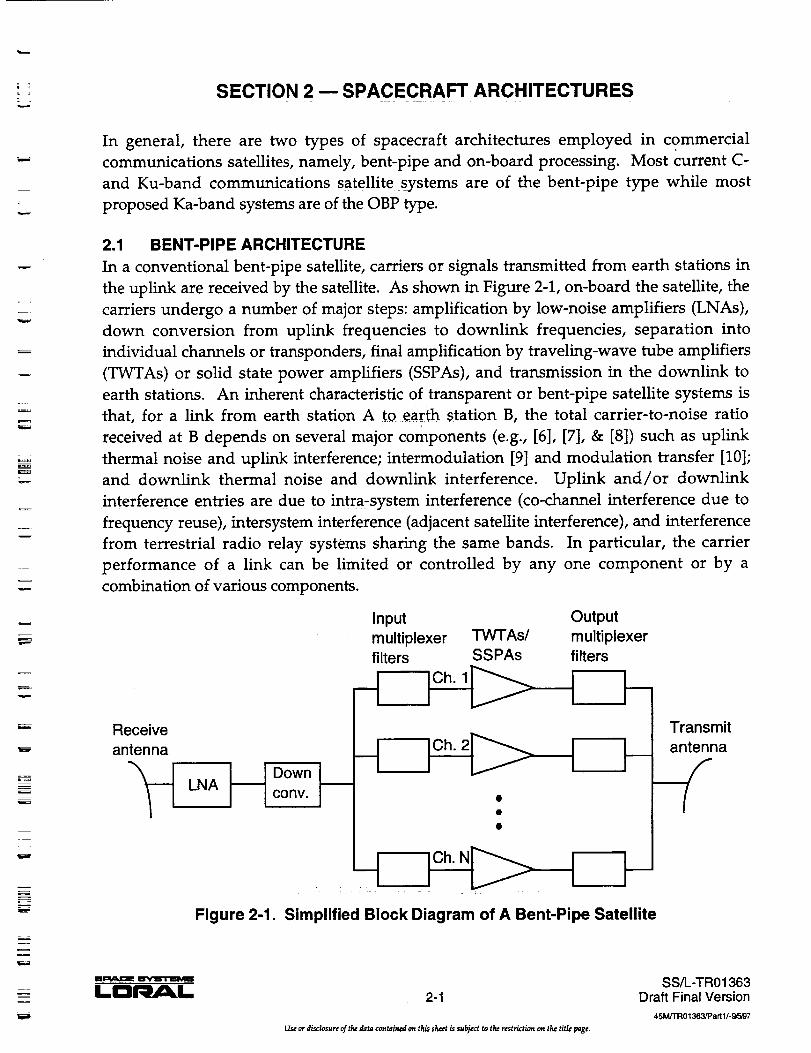
in a conventional bent-pipe satellite, carriers or signals transmitted from earth stations in
the uplink are received by the satellite. As shown in Figure 2-1, on-board the satellite, the
carriers undergo a number of major steps: amplification by low-noise amplifiers (LNAs),
down conversion from uplink frequencies to downlink frequencies, separation into
individual channels or transponders, final amplification by traveling-wave tube amplifiers
(TWTAs) or solid state power amplifiers (SSPAs), and transmission in the downlink to
earth stations. An inherent characteristic of transparent or bent-pipe satellite systems is
that, for a link from earth station A to earth station B, the total carrier-to-noise ratio
received at B depends on several major components (e.g., [6], [7], & [8]) such as uplink
thermal noise and uplink interference; intermodulation [9] and modulation transfer [10];
and downlink thermal noise and downlink interference. Uplink and/or downlink
interference entries are due to intra-system interference (co-channel interference due to
frequency reuse), intersystem interference (adjacent satellite interference), and interference
from terrestrial radio relay systems sharing the same bands. In particular, the carrier
performance of a link can be limited or controlled by any one component or by a
combination of various components.
Receive
antenna
LNA
Input Output
multiplexer TWTAs/ multiplexerfilters SSPAs filters
HOownk__cony. / •
Transmit
antenna
-<
M
Ul=l_a=m
LDI' L
Figure 2-1. Simplified Block Diagram of A Bent-Pipe Satellite
2-1
Use or disclosure of the data contained an this sheet is su_ect to the restriction on the title page.
SS/L-TR01363Draft Final Version
45 M/T'R01363/Pa rt 1/- _tr-a97

2.2 ON-BOARD PROCESSING ARCHITECTURES
OBP satellites are more complex than bent-pipe satellites. Benefits arising from the added
complexities are numerous [2]-[4], and vary as the degree of complexity is implemented in
a specific OBP design. Depending on network requirements, an OBP satellite (Figure 2-2)
can be designed to include a combination of capabilities such as demultiplexing/
multiplexing, demodulation/modulation, decoding/encoding, beam switching, baseband
switching (time slots or packets), etc. OBP communications payloads can be grouped into
three types as follows.
(1) In the first type, the main function of the payload is to route or channelize
(demultiplex/multiplex) traffic from upbeams (i.e., uplink beams) into downbeams
(i.e., downlink beams) according to certain operational network requirements. For
example, in the INTELSAT VI satellite-switched time-division multiple access
(SS-TDMA) system [11], [12], TDMA bursts arriving on various upbeams can be
routed by the microwave switch matrix (MSM) on board the satellite to various
downbeams according to specific switch state time plans. It should be noted that, in
this situation, the TDMA carrier link performance also depends on a number of
components as described in Section 2.1 since, once a switch state is established, the
transponders behave like bent-pipe transponders during that switch state duration.
(2) The second type refers to regenerative payloads in which uplink carriers are first
demodulated and decoded into baseband signals. These signals can then be further
processed, and encoded and modulated before transmission onto downlinks. Since
baseband signals are available on board the satellite, it is possible to implement
dynamic connectivity among all beams and channels (users) using a baseband
switch and a processor. The principal benefit realized with this architecture is the
complete isolation between uplink degradations and downlink degradations,
thereby improving substantially the carrier bit error ratio (BER) performance [2],
J
I
m
m
I
!
U
m
m
i
iuw
M
Receive
antenna
Hc o°vF-I OBP
Transmit
TWTA/SSPA antenna
H°U°nvDemultiplex/Multiplex
Demodulation/ModulationDecode/Encode
Beam switchingBasebana switching
Figure 2-2. Simplified Block Diagram of An OBP Satellite
2-2
Use or disclosure of the data contained on this sheet is subject to the restriction on the title page.
SS/L-TR01363Draft Final Version
45 M/TRO 1363/Part 1/-_,,97
w
J
E--.
(3)
[13]. Proposed Ka-band systems which utilize regeneration and baseband circuit
switching [3] include, for examples, the CyberStar [14] and Galaxy/Spaceway [15]
systems.
In the third type, regeneration and a more advanced form of baseband switching,
called fast packet switching, with capabilities similar to those of an Asynchronous
Transfer Mode (ATM) swich are utilized [3]. Here, the same benefit with respect to
the improvement of the carrier BER performance is also realized. A proposed Ka-
band system utilizing this architecture is the Astrolink system [16].
In this study, the two architectures evaluated are bent-pipe and regenerative with
baseband circuit switching. In particular, for the latter, in the uplinks, TDMA carriers will
access the satellite in the frequency-division multiple access (FDMA) mode; and, large
time-division multiplex (TDM) carriers will be transmitted in the downlinks. It should be
noted that only a high-level evaluation will be performed for these two architectures with
respect to rain fade compensation techniques since very little technical information was
provided in [14] and [15].
L:
t_
-::z
Bm
Em
m
m
LDr4._6 2-3
Use or dL_losurr of the data contained on tE@ sheet is sub_ect to the restriction on the title page.
SS/L-TR01363Draft Final Version
45M/TR01363/Part I 1-9,_,97

il
zg
r m
J
g
J
mm
II
zm
li
_m
w
z
Imini
L
=
m
z
r_==
E
i
SECTION 3 -- RAIN FADE CHARACTERIZATION
Propagation factors that affect Ka-band satellite links operating at moderate to high
elevation angles include:
• gaseous absorption
• cloud attenuation
• melting layer attenuation
• rain attenuation
• rain and ice depolarization
• tropospheric scintillation
Gaseous absorption, cloud attenuation, melting ia_er attenuation, and rain attenuation are
absorptive effects producing both signal attenuation and a proportionate increase in the
thermal noise received at the antenna port. Systems employing orthogonal polarization to
implement frequency reuse suffer from interference produced by rain and ice
depolarization. Tropospheric scintillation is non-absorptive and produce signal attenuation
as well as enhancements. Due consideration must be given to the different impairment
factors when designing fade mitigation schemes, in this respect, fade rates, fade durations,
and frequency scaling behavior of fading mechanisms are of special importance. A brief
review of the various impairment factors are presented below.
3.1 GASEOUS ABSORPTION
Compared to other absorptive effects gaseous absorption arising from oxygen and water
vapor present in the atmosphere is relatively small. Absorption due to oxygen is nearly
constant and that due to water vapor varies slowly with time in response to variations in
temperature and humidity [17]. Gaseous absorption at 5°C and 25°C as a function of
relative humidity is shown in Figures 3-1 and 3-2 for typical Ka-band up- and down-link
frequencies; elevation angle is 40 ° . As evidenced, the gaseous absorption increases with
the relative humidity as well as the temperature. Closeness of the down-link frequency to
the water vapor absorption line at 22.2 GHz makes the absorption at the down-link
frequency exceed that at the up-link frequency. This occurs when the water vapor
absorption is significantly larger than the oxygen absorption. It is seen that for moderate
elevation angles the gaseous absorption amounts to less than 1.5 dB under most conditions.
The fade ratio between the two frequencies are also shown in the figures. The fade ratio is
a function of both humidity and temperature and varies approximately between 1.5 for
complete dry conditions and 0.8 under high humidity conditions. For practical purposes
the ratio can be considered equal to unity.
w
3-1
Use or disclosure of the data contained on this sheet is subject to the restriction on the title page.
SS/L-TR01363Draft Final Version
45fWTR01363/Part II- 96,97

1.6
1.4
1.2
-= 0.8
._0.6
< 0.4
0.2
Figure 3-1.
Gaseous Absorption at 25°C
k ; i i 20 GHz: =="''30 GHz i
---_ade Ratio ]
20 40 60 80 I00
Relative Humidity (%)
Gaseous absorption at 20 and 30 GHz; temperature:
5°C, elevation angle 40 °
g
I
_i
M
I
IB
Absorption (dB)
Figure 3-2.
16
,4\1.2 _.
0.8
0.6
0.4
0.2-f
0
0 20
Gaseous Absorption at 25°C
_20 GHz
_30 GHz
mmmm_ade Ratio
J
40 60
Relative Humidity (%)
80 I00
Gaseous absorption at 20 and 30 GHz; temperature:
25°C, elevation angle 40 °
m
zElmI
I_e_a_=m =Pf_l'rt_Ul6
LE3_L 3-2
Use or disclosure of the data contained on this sheet is subject to the restriction on the title page.
SS/L-TR01363Draft Final Version
45 M,rFR01363,'Pa r t 1/- 9,'5,97m

L
z
r
m
i
m
3.2 CLOUD ATTENUATION
At Ka-band frequencies clouds containing liquid water can produce both signal attenuation
and amplitude scintillations [18]; ice clouds, in general, do not produce these effects. The
small size of cloud particles relative to the wavelength makes cloud attenuation essentially
a function of cloud temperature and the integrated liquid water content along the
propagation path. Figure 3-3 show the relationship between cloud attenuation, frequency,
and cloud temperature. The specific attenuation coefficient shown is defined as the specific
attenuation (dB/km) for a liquid water content of 1 gm/m 3. Table 3-1 shows average
properties of several cloud types and the levels of expected attenuation for an elevation
angle of 40 °. Attenuation levels are calculated assuming a uniform distribution of the liquid
water within the cloud. It is seen _at significant amounts of cloud attenuation can be
expected at the up-link frequency of 30 GHz. The fade ratio between two frequencies is
approximated by [19]:
..... A.__.L=(f_2
A2 [,f2) (3-1)
where A 1 are A 2 are attenuation (dB) at frequencies fl and f2, respectively.
Although reliable information on fading rates associated with clouds is generally lacking,
fade rates are thought to be relatively small (in the range 0.1 to I dB/min).
-._ _C"
0 °CIO°C
Specific A Itenuation
Coefficient(dB/km)/(grn/m "_)
0.4 /
0.2
I0 15 ?0 5Frequency (GHz)
_0
Figure 3-3. Specific Attenuation of Clouds as a Function of
Frequency and Temperature
m
ls_n_m I_'YB'I"EMa
LE3_L 3-3
Use ordisclosureof the data containedon this sheetis subject to the restriction on the titlt page.
SS/L-TR01363Draft Final Version
45M/TR01363/Part11-_/97

Table 3-1. Average Properties of Different Cloud Types
Cloud Type
Cumulus
Stratus
Stratocumulus
Altostratus
Density(g/m3)
1.0
0.15
0.55
0.4
Vertical Extent20 GHz
Attenuation(dB)(km)
1.0 - 3.5
0.5 - 2.0
0.5 - 1.0
2.5 - 3.0
0.8
0.4
0.6
0.4
30 GHzAttenuation
(dB)
1.8
0.9
1.3
0.9
=_
m
R
J
3.3 RAIN ATTENUATION
Rain attenuation is the dominant propagation impairment at Ka-band frequencies. Rain
attenuation is a ftmction of frequency, elevation angle, polarization angle, rain intensity,
rain drop size distribution and rain drop temperature. Fade durations and rates are closely
correlated with the rain type; e.g. stratiform rain are conducive to longer fade durations
and slower fade rates. Frequency scaling of rain attenuation is largely determined by the
raindrop size distribution and the rain temperature. As a first order approximation, the
same frequency scaling relationship given in equation 3-1 may be used for rain as well. A
more rigorous scaling law can be found in [17].
Figure 3-4 shows the distribution of signal attenuation observed at 20.2 and 27.5 GHz at
Clarksburg, MD. The data were collected using the beacon signals on the ACTS satellite
[20]; elevation angle is 39 ° . Total path attenuation that include gaseous absorption and
other clear-air effects are included in the distributions. Also shown in the figure is the rain
rate distribution. It is seen that the annual raining time for the measurement site is around
5%. Annual time percentage for which rain attenuation is present along the observation
path is somewhat higher due to the fact that rain attenuation is produced by the presence
of rain along the satellite path and the rain rate distribution pertains only to a point
measurement near the earth station antenna. Due to the presence of other factors such as
cloud attenuation, raining time along the path can not be easily discerned. As shown in the
figure, fade depths at 27.5 GHz under moderate elevation angles exceed 20 dB for 0.1% of
an average year. Fading becomes worse for low-elevations and/or severe rainfall climates.
Figure 3-5 shows the fade distributions at 20 GHz for different rain climates as defined by
the ITU-R; elevation angle is 40 o. The distributions have been derived using the ITU-R rain
attenuation prediction model. Both fade durations and fade rates associated with rain
attenuation are found to be distributed in a log-normal fashion; these are discussed in
detail in subsection 3.8 on fade dynamics.
wIM
I
m
g
m
M
g
g
!i1_¢k¢21 m'Y1B'¢_6
I.I¢I_L 3-4
Use or disclosure of the data contained on this sheet is subject to the restriction on the title page.
SS/L-TR01363Draft Final Version
45MJTR01363/Part 1/-_u97 I

Cumumative Distribution of 20.2 and 27.5 GHz Attenuation;Clarksburg, MD; March, 199_ - February, 1995
w
=,E
m
50
45
40
35Attenuation (dB)/ 30
Rain Rate 25
(mm/hr) 20
15
10
5
0
0.01
I IIIII"_ IJlll
Jllll_111
.. "Nlll,,, a,i,w,_L
i]'l,ifi_"_II1_!!1111IIIII1
I IIII-I- 20 GHz
I 111.,_27 G_IIIII II II-'- Rai_e.at_IIIIIII lliiiI IIIIII I III1[IIII111 IIIII
,k_'_d I IIIII IIIIII• I
' _ /i_i'._,_ _11111
IIIIIIIIIIIIIIIIIIIIII111IIIIII11111_IIII1{
1,,i0.1 I I0 I00
Percent Time Ordinate Exceeded
Figure 3-4. Attenuation and Rain Rate Cumulative Distributionsfor Clarksburg, Maryland. Elevation angle 39°
Attenuation(dB)
50-
45
40
35
30
25
20
15
,oJ
5
0
P.0I 0.1 10 I00
Percent Time Ordinate
Figure 3-5. Rain Attenuation Distribution at 20 GHz for Different
Rain Climates; Elevation Angle 40 °
Rain Zone
m
---,I--B
--l--D
--I_--F
--X--H
-,¢---K
-@--M
-.4.-p
_ u'v'l_r'rlml_lg
3-5
Use or disclosure of the data contained on this sheet is subject to the restriction on the title page.
SS/L-TR01363Draft Final Version
4 SM/TR01 _163/Par t 1/- 9,eB7
3,4 MELTING LAYER ATTENUATION
The melting layer is the region around the 0°C isotherm where snow and ice particles from
aloft melt to form rain. The presence of a well defined melting layer or radar bright band is
mainly associated with precipitation from stratiform clouds and for low rain rates. The
width of the layer is of the order of 500 m. Specific attenuation in the melting layer,
however, is expected to be higher than that in the rain below. Therefore, under light rain
conditions, melting layer attenuation may become a significant factor in the total path
attenuation; typically, fade levels up to about 3 dB can be expected at 30 GHz [21]. Fade
rates are similar to those produced by rain under low fade conditions.
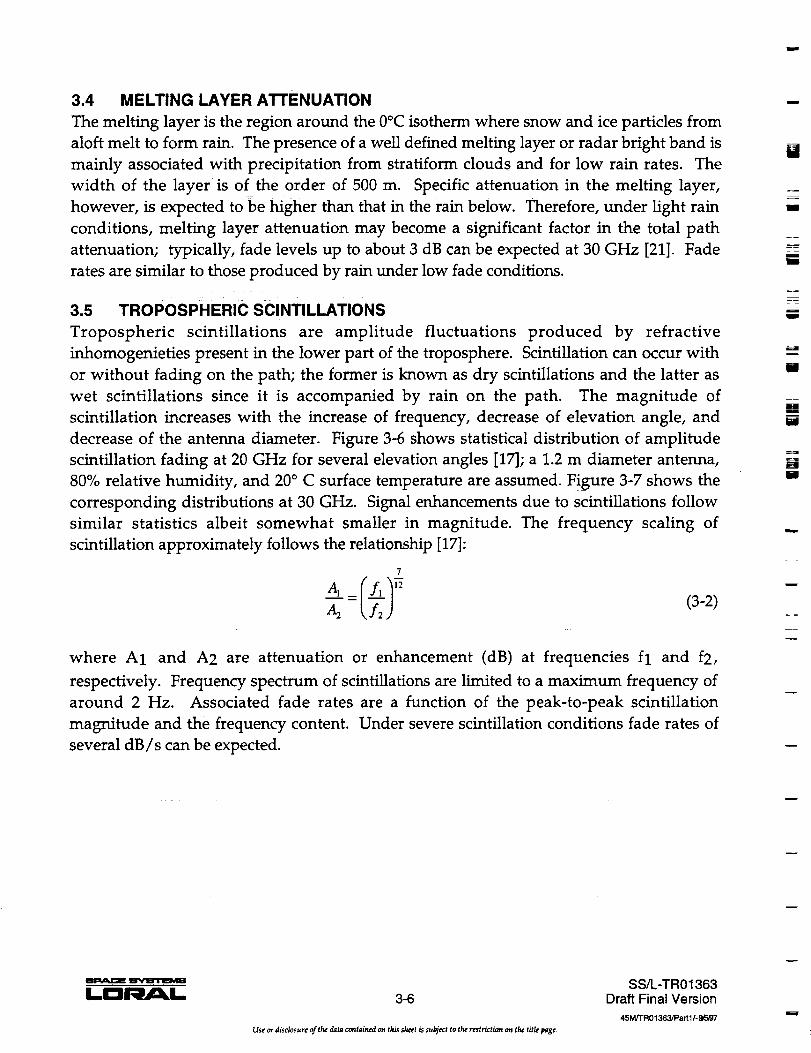
3.5 TROPOSPHERIC SCINTILLATIONS
Tropospheric scintillations are amplitude fluctuations produced by refractive
inhomogenieties present in the lower part of the troposphere. Scintillation can occur with
or without fading on the path; the former is known as dry scintillations and the latter as
wet scintillations since it is accompanied by rain on the path. The magnitude of
scintillation increases with the increase of frequency, decrease of elevation angle, and
decrease of the antenna diameter. Figure 3-6 shows statistical distribution of amplitude
scintillation fading at 20 GHz for several elevation angles [17]; a 1.2 m diameter antenna,
80% relative humidity, and 20 ° C surface temperature are assumed. Figure 3-7 shows the
corresponding distributions at 30 GHz. Signal enhancements due to scintillations follow
similar statistics albeit somewhat smaller in magnitude. The frequency scaling of
scintillation approximately follows the relationship [17]:
7
A,_- = _,f-_z) (3-2)
where A1 and A2 are attenuation or enhancement (dB) at frequencies fl and f2,
respectively. Frequency spectrum of scintillations are limited to a maximum frequency of
around 2 Hz. Associated fade rates are a function of the peak-to-peak scintillation
magnitude and the frequency content. Under severe scintillation conditions fade rates of
several dB/s can be expected.
w
i
U
L--
i
mg
u
I
n
m
m
i
w
= =
3-6
Use or disclosure o_ th¢ data contained on this sheet is subject to tht restriction on the title pag¢_
SS/L-TR01363Draft Final Version
45M/TR01363/Part 1t- 9,597m
=
= =
w
w
E
30 GHz Scintillation Fading Distribution
i I I IIii / _ .--_--!o_L4- f ÷ -; ]- -___ +20 ° i-_-
i ', Ii r_ot f _ '! o
0.1 l I0
Percent Time Ordinate Exceeded
Figure 3-6. Cumulative Distribution of Scintillation
Fading at20 GHz
5 ¸
II]Ill
Fade Depth (dB) ._ _ ,_
I --
0.1
30 GHz Scintillation Fading Distribution
,,vaf,otH,,_ 10 o
•--6--20 o
X 40 o
_I1(--- 50o
PercentTime )rdinate Exceeded
Figure 3-7. Cumulative Distribution of Scintillation
Fading at 30 GHz
l0
=
m_
r===
M
ll_/=tJ_E _
LIE3RM_L 3-7
Use or disclosure of the data contained on this sheet is subject to tht restriction on the title page,
SS/L-TR01363Draft Final Version
45M/TR01363/Part 1/-gr-J37

3.6 RAIN AND ICE DEPOLARIZATION
Satellite systems employing frequency re-use by means of orthogonal polarization may
suffer from interference through coupling between wanted and unwanted polarization
states. Such coupling arises from antenna imperfections and atmospheric depolarization
caused by precipitation particles. Non-spherical particles such as spheroidal rain drops
and needle or plate like ice particles can produce coupling between orthogonal polarization
states. Depolarization is a function of the polarization state, elevation angle, and the
frequency. In the case of linear polarization, depolarization increases with the polarization
tilt angle with respect to the local horizontal, and reaches a maximum when the tilt angle is
45 °. Depolarization for a circularly polarized signal is same as that for a linearly polarized
signal having a 45 ° tilt angle. At Ka-band frequencies rain depolarization becomes
significant only at fade levels in excess of about 10 dB. On the other hand ice
depolarization may be experienced without significant fading along the link.
Rain and ice depolarization may be predicted using empirical techniques such as the one
recommended by the ITU [17]. Figure 3-8 shows the distribution of the cross-polar
discrimination (XPD) at 20 and 30 GHz due to atmospheric precipitation particles; the XPD
is defined as:
..,, ( signal power in the wanted polarizationXPD = lu log/ .....
signal power in the unwanted polarization ) (3-3)
The figure pertains to an elevation angle of 40 °, circular polarization, and a rain climate
typical of a US mid-Atlantic location. A comparison of rain attenuation levels shown in
Figure 3-4 with depolarization levels in Figure 3-8, it may be surmised that for availability
time greater than about 99% depolarization is of secondary importance compared to
fading. However, when fade compensation is applied through power control the
interference caused by depolarization increases proportionately to the amount of power
control applied, and due care must be taken to avoid excessive interference.
3.7 COMBINED EFFECT OF PROPAGATION FACTORS
The preceding subsections outlined the individual propagation impairments affecting Ka-
band satellite links. In general, most of these impairments can occur simultaneously. This
is illustrated in Figure 3-9 where the time series of a fade event recorded at Clarksburg,
MD, using the ACTS beacon signals are shown. In Figure 3-10 power spectrum of the time
series at the two frequencies are shown, and Figure 3-11 shows the ratio of the spectral
components at the two frequencies (ratio of logarithmic value of spectral components). It is
seen that different propagation factors can be easily identified through the spectral ratio.
The lowest frequency components of the spectral ratio are identified with the gaseous
m
g
m
ii
m
l
!
m
M
w
Ilmdlld_g
LCI_L 3-8
Use or disclosure of the data contained an this sheet is subject to the restriction on the title page.
SS/L-TR01363Draft Final Version
45M/TR01363_art 11-gF_J7wm

i
I
50
40 IIlllIllll
Depo larization t_
(dB) 20
iIIt I0.01
Ii1111IIIIII
II]lll0.1 1
Percent Time Ordinate Not Exceeded
IIIII..... IIIII
I]IIIIIIIII
10 100
1_2°°"zI30 GHz
Figure 3-8. Distribution of XPD at 20 and 30 GHz
18.00 19.00 20.00
Time - UT
:
m -lO
._ -15
!___o.--_o?_;r_
-25
-30 "
16.00 17.00
,j,
k_21.00 22.00
Figure 3-9. Rain event observed at Clarksburg. Signal attenuation on 20.2 and
27.5 GHz ACTS beacon signals are shown; elevation angle 39 °
..=.
UKJ
IlI=_IE gPdlI'f'lEl_g
3-9
Use or disclosure of the data contained on this sheet is subject to the restriction on the title page.
SS/L-TR01363Draft Final Version
45 M/TR01363/Part 1/-9,5,97

Powcr
DensitydB/Hz
- fill ,....., ,,
IIII 1_IIII
- IIII I II0.1
0.001 O.Ol O.l
Fouricr frequency (Hz)
w
!
M
i
i
w==7,
l
Figure 3-10. Power Spectra of the Fading Event Depicted in Figure 3-9
1.5
.
PowerDensityRatio
0.5
gasl
!i
IS
_kkt llJllll Ii+_IIIA+_ _tll. lJ,J,IIIII+ +IVflll_,,J+IJilIII
IIIII.IIIII11111
0
0.001 O.Ol 0.1
I[llltr+wIeMlll
lllllll IIIIIIIII IIlllllll II
Fourier Frequency (Hz)
IIIiiIIIIIIIIIIIIII111IIIIIIIIIIII
I
Figure 3-11. Ratio of Spectral Components at 27.5 and 20.2 GHz
!!¢=_¢_C=E EiV'IFrlEI_I_
I..l'llqM_l- 3-10
Use or disclosure of the data contained on this sheet is sub_ect to the restriction on the title page.
SS/L-TR01363Draft Final Version
45M/TR01063/Part 11- 9_97

m
--=2
absorption; mid frequencies are associated with cloud_ and rain attenuation, and higher
frequencies are produced by scintillation activity. As such, frequency domain separation of
propagation factors can be gainfully employed when implementing fade mitigation
techniques.
3.8 FADE DYNAMICS
Dynamics of fade events are of importance in the design and implementation of fade
mitigation techniques employing power control, diversity, coding, and resource sharing.
In addition, they need to be considered when specifying performance objectives of digital
networks employing satellite links. Fade duration, or the time interval during which the
signal attenuation exceeds a given threshold, intervals between fade episodes, intervals
between fade events, and the rate of change of attenuation are the most important dynamic
features relevant to system modeling.
Within a precipitation event, the fade level varies considerably, crossing a given fade
threshold several times over a relatively short time interval; precipitation events
themselves are separated by a longer time span as illustrated in Figure 3-12. A
precipitation event starts when the fade level exceeds a given threshold and ends when the
fade level falls below the threshold and is followed by a long gap during which the fade
level is closer to the clear-air value.
Within the event, there may be several short duration peaks separated by several short
gaps. The peaks are called fade episodes and the gaps are known as inter-episode gaps or
inter-fade intervals. The relatively longer time interval between fade events is the inter-
event interval. Tropospheric scintillations often accompany precipitation events, and the
m
z
Fad
Fade
episodes
IJ.,ml
Figure 3-12.
Fade
duratio_
-4--------4_- -qt---I_Interfade
interval A
Precipitation event
Fade A
_ 1 Fade threshold
Time
Inter-event interval Precipitation
event
Features Commonly:0sed incharacterizing Precipitation Events _
l_ lii'VIB'rlEI_B
3-11
Use or disclosure of the data contained on this sheet is subject to the restriction on the title page.
SS/L-TR01363Draft Final Version
45M/TR01363_a rt1/- 9F0_7

above features need to be characterized both in the presence and absence of scintillations.
Scintillations are relatively fast variations in the signal amplitude and these can be
separated from slower variations produced by precipitation particles using a low-pass
filter. Filter time constants of the order of 20 to 60 seconds appear to be adequate for the
purpose [20].
3.8.1 Fade Duration
In general, fade duration is a function of frequency, elevation angle, and the rain type. At a
given fade threshold the fade duration will increase with an increase of frequency and a
decrease of the elevation angle. Experimental evidence show that these dependencies
approximately follow the rain attenuation dependence on frequency and elevation angle
[23]. Thus, the frequency dependence of fade duration at a fixed elevation angle is
approximately given by:
total number of fades with A > x dB at fl =(fl'_ 2/--I
total number of fades with A > x dB at f2 \ f2 J (3-4)
where A is the fade depth (dB) and x is the threshold (dB) at which the fades are counted
and f is frequency. A more rigorous frequency scaling law may be found in [17]. The
elevation angle dependence at a fixed frequency may be approximated by:
total number of fades > A dB at 01 sin 0 2
total number of fades > A dB at 0 2 sin 01 (3-5)
where 0 is the elevation angle.
The elevation angle dependence shown above is expected to hold only for moderate to high
elevations where fading is produced by individual rain cells. At low elevation angles more
than one rain cell often contributes to the fading process, thus leading to a more complex
elevation angle dependence.
The role of the rain type in influencing fade duration stems directly from the average dwell
time of rain structures. Wide spread rains tend to have longer dwell times compared to
thunderstorm rains.
The average duration of fades exceeding a given threshold appears to be independent of
the threshold level. This is due to the fact that the number of fades increase with the
decrease of the fade threshold without any discernible relationship between the two
parameters. The larger time percentage for which a lower fade threshold is exceeded is
distributed among a larger number of fades, and the lower time percentage at a higher fade
m
m
w
m
U
I
[]
m
m
F
w
IlIn_A_IB liYUTIB_g
t_D_t_ 3-12
Use or di_losur¢ of tlu_ data contained on this sheet is subject to the restriction an the title page.
SS/L-TR01363Draft Final Version
45 M,tTR01363/Part 1]- _ir-o,g7M :

F =
G_
w
threshold is distributed among a smaller number of fades. An example of average fade
duration is given in Figure 3-13. An average fade duration of approximately 2 min. for
most fade thresholds is evidenced in Figure 3-13 [20]. This seems to be typical for most
paths and climates with the exception of those regions that are subject to extremely severe
and widespread events such as typhoons. The spread of fade duration around the average
value increases with the decrease of the fade threshold. As an example, it is common to
observe fades lasting more than an hour at a threshold of 3 dB; on the other hand, a fade of
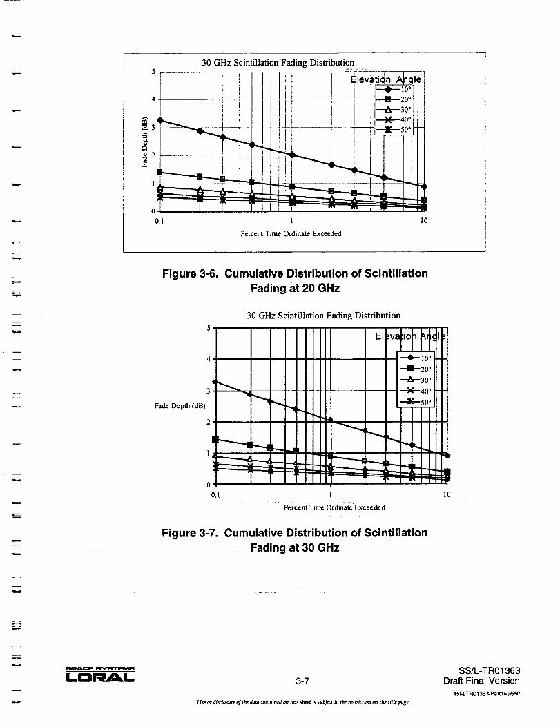
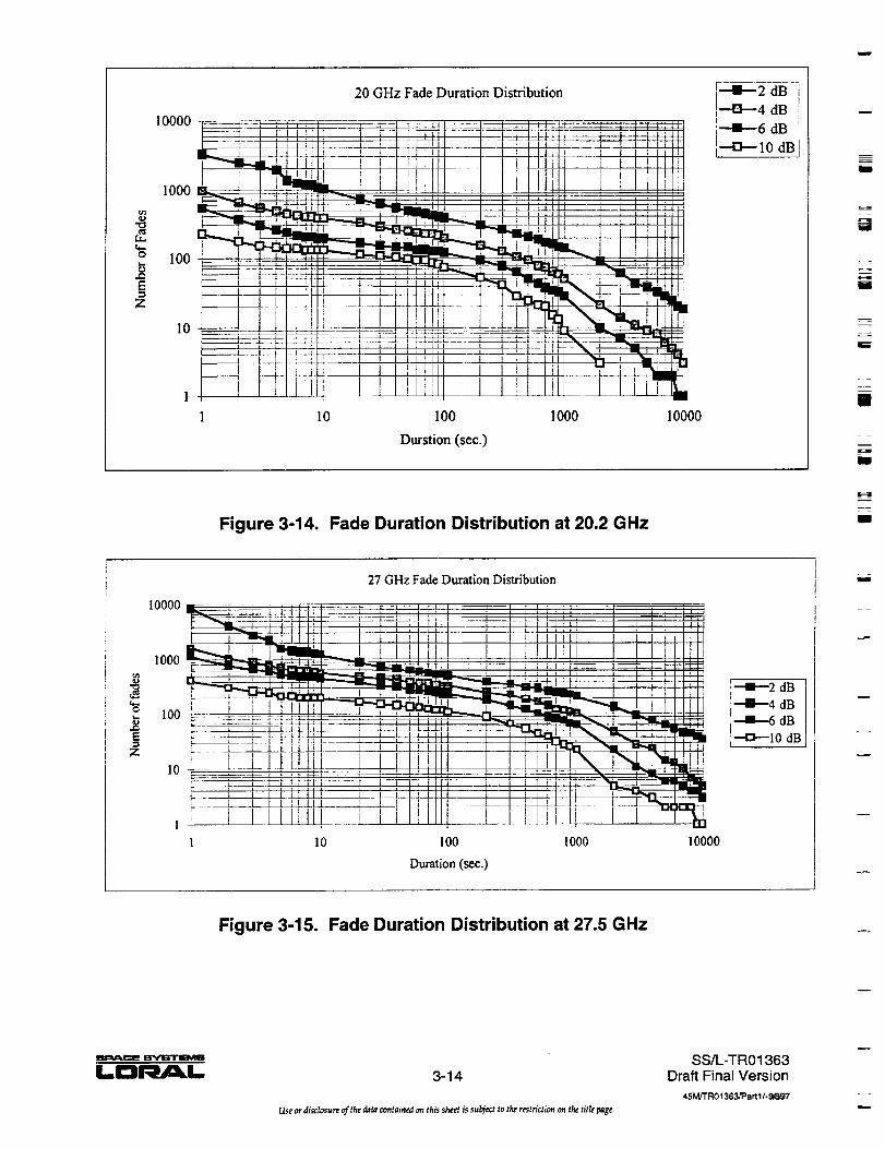
20 dB is less likely to last more than two or three times the average value. This is illustrated
in the fade duration statistics shown in Figure 3-14 and 3-15 for 20.2 GHz and 27.5 GHz,
respectively.
The measured data indicate the duration of fades exceeding a given threshold to have a
log-normal distribution for longer duration fades composed mainly of rain induced fades.
Shorter duration fades, produced largely by tropospheric scintillations, can be represented
by a power-law distribution [24].
3.8.2 Inter-Fade and Inter-Event Intervals
Information on interfered intervals is important in applications such as diversity switching
in which excessive switch occurrences can have a detrimental effect on system
performance. Inter-event intervals, which pertain to the return period of precipitation
events, are of importance in network management and reallocation of resources on a larger
scale.
20O
|6O
,° /\FadeAverage 120 _ _Duration _oo
/_ \/6O
/ \/o /
I
0
0
Figure 3-13. Average Fade Duration at 20.2 GHz
m_
3-13
USe or dJsclosur¢ of the data contained orl this sheet is subject to the restriction1 on tl_ lille pagt.
SS/L-TR01363Draft Final Version
45 M/"r'R01363/P art 1/- 9_/:J7
gt_
L_
O
Z
20 GHz Fade Duration Distribution
lOOOO __:__ _ . - .
1000
100 _ ......
1 10 100 1000 10000
Durstion (see.)
+2 dB i--0----4 dB i+6dB !
--43---10 dB I
m
=_
U
b
W
Figure 3-14. Fade Duration Distribution at 20.2 GHz
I27 GHz Fade Duration Distribution
-- -._t_ _-_-_--7__-LL_ L__SIES ÷ , _ , _ I i t , : I r : i : t i i i I 7 J
i
_AIi_ i i J i'iii_ i ' i iiiili _ i i i I____2! [!! !! ! t! !1_1 !! Ill,l!
l ' _L I_ , I -....!1-.--4 dB
[ l I ! i I I * I Ill I ! i , * t t t
5 I i. illlt_._t t! !illll ...../_J__!__]_ _i,._:,___10 F ! i J i i l ),! ..... , _ ' : ] i lit ..... I----N- r-,_T-,____
__ I I I I I I i I t :
: ! I I J l II Ill ......L 1 i I[lll ___J._1 l!l_lj II _-_1 10 100 1000 10000
Duration (sec.)
K==i
Ul
u
Figure 3-15. Fade Duration Distribution at 27.5 GHz
LI'II_/_I. 3-14
Use or disclosure of the data contained an this sheet is subject to the restriction on the titIe page.
SS/L-TR01363Draft Final Version
45Mf'rR01363]Part 1/-9,_97
e,..

=
--mw
o
In general, rain induced inter-fade intervals and inter-event intervals are log-normally
distributed [24]. Short duration inter-fade intervals resulting from tropospheric
scintillations, however, are expected to follow a power-law form as found with the short-
term fade duration. Figures 3-16 and 3-17 show inter-fade interval distributions derived
from data collected using the ACTS beacon signals at 20.2 and 27.5 GHz; elevation angle is
40 ° . It can be seen that the slope of the distribution changes with the fade depth. Higher
fade thresholds are characterized by longer intervals compared to those at lower fade
thresholds.
Frequency and elevation angle scaling of inter-fade intervals may be attempted using the
relationships given under fade duration.
3.8.3 Rate of Change of Attenuation
In a manner similar to rain fade duration statistics, the distribution of the rate of change of
attenuation appears to be log-normal with a median of about 0.1 dB/s. Little difference has
been observed between the positive-going (fading) and negative-going (recovering) slopes
of the rate of change of attenuation for integration times of 10 s or more. In most
experiments reported to date, the average fade slope does not appear to depend
significantly on the fade level, with a maximum fade rate of about 1 dB/s being reported
for integration time constants of the order of 10 s. Much higher fading rates are observed
with integration times below 10 s and these are associated with scintillation activity.
100000
10000
•"v 1000
1000
= 10Z
20 GHz Inter-fade Duration Distribution
1 I 0 100 1000 10000 100000 1000000
Inter-fade Interval (sec.)
--!---2 dB t
_4 dB
----!1---6 dB [--o-10 dB1
Figure 3-16. Inter Fade Interval Distribution at 20.2 GHz
=
3-15
Use or disclosure of the data contained on this sheet is subject to the restriction on the title page.
SS/L-TRO 1363Draft Final Version
45 M/TR01363/Part 1/-9/_97

100000
-_ 10000P
.
1000
_- I000
E lOZ
27 GHz Inter-fade Duration Distribution
--._ __,____._ _ ,, ,__ _______i_ ' ILLLLL /I ! I'J I 111111 I ! Illlld I _ I_[Lt2! .... / __J.Ak. i t;IIII !ill ill I llllllJ !!!l[ll'_! Ihlllt_J /ill_.__.-- i ,,4 i , , ,,¢__ _i.LZt-J-_,- i ', ',illp _ : ',il
L_-- I I i![ t I Ilill'l 1 i i] Ill l I _ 1
'_.._4._[i I ,,'T_Iik___LF4]I! I_ Ill/:; /IIii
| i !'lll'l / I IlL _LL__jIJi!L__]_.IIILL_,'__I I ill 'l __m.L.LJ_
i i!iii[i _ ItlJ I i!l I I I!] t!_ i : _I i L _!1"11_
Jil I { _ _ _ I'I!i1_,' t llllli I lill!! Iililli; I!!11 ii ill
1 10 100 1000 10000 100000 1000000
Inter-fade Interval (see.)
+2 dB
_4 dB
+6 dB
--O-- l 0 dB,
E
I
i
l!l
I
m
I
Figure 3-17. Inter Fade Interval Distribution at 27.5 GHz
Figures 3-18 and 3-19 show the cumulative distribution of fade slopes at 20.2 and 27.5 GHz
for different fade thresholds. It is evident that the fade slope distributions are not sensitive
to the fade threshold. Figure 3-20 shows a histogram of fade slopes at 20.2 GHz illustrating
the symmetrical behavior of positive and negative going slopes.
m
i
m
J
Distribution of Fade Slopes at 20.2 GHz
_ i Attenuation
•_ !--_-6dB!--/_--6-8aB["-'X'_ 8- lOde
0.1
0 02 0.4 0.6 0.8 1 12 1.4
Fade Slope (dB/s)
Figure 3-18. Cumulative Distribution of Fade Slopes at 20.2 GHz
w
I..aI'_M_L 3-16
Us¢ or disclosure of the data contained on this sheet is subject to the restriction on the title page.
SS/L-TRO 1363Draft Final Version
45 M/'r'R01363_anl l-_BgJ7
i

1001
=" 0.1
Distribution of Fade Slopes at 27.5 GHz
0.5
Fade Slope (dB/s)
1.5 2
""0"--2 - 4 dB
I'--E]_4- 6 dB
I'_'_ 6 - S dB
I,_-X-_ 8 - lOdB
Figure 3-19. Cumulative Distribution of Fade Slopes at 27.5 Ghz
10OO0O
10OOO
1000
dZ
Fade Slope Histogram
100
lo!1:-1.5 -1 -0.5 0 0.5 1 1.5
Fade Slope (dB/s)
Figure 3-20. Fade Slope Histograms at 20.2 GHz
Attenuation
2-4d8 I
M
I--DI A I-- 3-17
Use or disclosure of the data contained on this sheet is subject to the restriction on the title page.
SS/L-TRO 1363Draft Final Version
45M/TR01363/Part 1/- 9/&97

3.9 RAIN FALL CORRELATION OVER LARGE AREAS
Rain fade compensation implemented on the basis of shared resources must be designed
with an understanding of the simultaneity of rain fading across the satellite coverage area.
Although detailed information on simultaneous rain fading on multiple satellite links
across a large area is not easily modeled, rainfall patterns over extended areas can be
studied to gain sufficient knowledge to size additional resources required for fade
compensation.
Meteorological data on hourly precipitation from several thousand stations scattered
throughout the continental USA were analyzed to derive rain fall correlation over extended
areas. Figures 3-21, 3-22, and 3-23 show the joint probability of rain for three cities:
Cleveland, OH, Los Angeles, CA, and Washington, DC.
m
M
w
I
I
10 ,.
"K .
Joint Probability of Hourly Rainfall Exceeding R for Cleveland, OH,
and a Second Site at a Distance D; R o: Rainfall at Cleveland, R l: Rainfall at Second Site
T.
Percent Probability -- _ _-
OA .-
0.01
,, |, ,,
--4--R = 0.0I mm/h
-m-"R = 2.5 mm/h
"-_-R = 5.0 mm/h
_R = 10 mm/h
0 500 1000 1500 2000 2500 3000
Distance D (kin)
Figure 3-21. Joint Probability of Rainfall Exceeding Specified Threshold
as a Function of Site Separation for Cleveland, OH
i
Ill
m
M
B
===_
!11
D
BPI_.C=m E_"_B'FEEarUlS
I_I"JI_/_L 3-18
Use or disclosure of the data containesl on this sheet is subject to the restriction on the title page.
SS/I_-TR01363Draft Final Version
45M/TR01363/Pa rt 1/-9_37
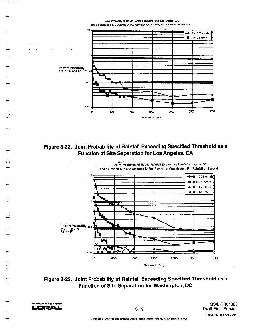
lO
1
Percent Probability(Ro >= R and R1 >= R)I
0.1
O.Ol
JointPrd:_0_tyd _ RainfalEx_ Rfor los Angeles,CA,
anda SecondSite at a DistanceD;,Ro: P,_J at LosAngeles,RI: Rairt'aJIat SecondSite
Z 5 mm/h
=
f
0 500 1000 15(30 2000 2500 3000
Di_=nceD (km)
w
w
=
z
w
Figure 3-22. Joint Probability of Rainfall Exceeding Specified Threshold as a
Function of Site Separation for Los Angeles, CA
Percent Probability 01_1o >= R and
>: R)
10.
Joint Probability of Hourly Rainfall Exceeding R forWashington, DC,
and a Second Site at aDistance D_ R0- Rainfall at Washington, RI: Rainfall at Second
-i
•-O--R = 0.01 mm/h
i -I--R = 2.5 mmlh
-.A--R = 50 mm/h
-_-R = 10 mm/h
0 500 1000 1500 2000 2500 3000
Distance D (kin)
Figure 3-23. Joint Probability of Rainfall Exceeding Specified Threshold as a
Function of Site Separation for Washington, DC
l.¢:31_h¢_1. 3-19
Useordisclosure o[ the data contained on this sheetis subject to the restriction on the titlepage.
SS/L-TRO 1363Draft Final Version
45M/T'R01363/PartI/- 9/_7

3.10 ANTENNA WETTING
In addition to rain fading, wetting of the antenna reflector surface and the antenna feed
window can produce additional signal attenuation [25]. Signal attenuation can be
especially severe at Ka-band frequencies. Antenna wetting effect can be modeled using
geometrical optics techniques [26]. Figure 3-24 shows the signal attenuation at 20 GHz due
to antenna reflector wetting as a function of the rain rate for an elevation angle of 40 ° and
80 °. A reflector diameter of 1.8 m and a smooth reflector surface are assumed in the
calculation. Signal attenuation at 20 GHz due to feed wetting is shown in Figure 3-25.
Figures 3-26 and 3-27 show results for 30 GHz. It is seen that attenuation due to feed
wetting is significantly higher than that due to reflector wetting. However, application of a
hydrophobic coating on the feed window can significantly reduce the signal loss. On the
other hand significant levels of attenuation may be encountered for reflector wetting when
the reflector surface is not smooth as demonstrated by the ACTS propagation
measurements. Fade mitigation techniques must account for the antenna wetting effects.
The antenna wetting contribution can be considered an error term when measuring the
fade on the satellite link.
m
zmu
I
BIw_
g
0 ¸
-0.5
-1
Rdative
Gain (dB)
-1.5
AntennaGain R_uction Due toReflector
-2
0 20 40 60 80 100
Rain me (ram/h)
Figure 3-24. Antenna Reflector Wetting Loss at 20 GHz
gm
I.,I:31qM L 3-20
Use or disclosure of the data contained on this she_ is subject to the restriction on the title page.
SS/L-TR01363Draft Final Version
45M/rR01363/Part 1/- 9/1_97
m

wFeed Window Wetting Loss
Feed Loss at 20 GHz
F
=--.
Relative C_n (dB)
-0.5
-I .5
.-,,.,.
Elevation Angle
--40 °
_80 o
-3.5
0 10 20 30 40 50
Rain Rate (nan/h)
Figure 3-25. Antenna Feed Wetting Loss at 20 GHz
w
.==
w
w
Relative Gain (dB)
-1.5
-2
Antenna Gain Reduction Due to Reflector We_ting;
Reflector Loss at 30 GHz
Elevation Angle
0 20 40 60 80 1O0
Rain rote (mm/h)
Figure 3-26. Antenna Reflector Wetting Loss at 30 GHz
m
_r-J_ U',_eEFrlz_MB
LE3Rt_L 3-21
Use ordisclosure of thedata contained on thissheetissubject tothe restrictionon the title page.
SS/L-TR01363Draft Final Version
45M,,TR01363JPart11-9b_9'7
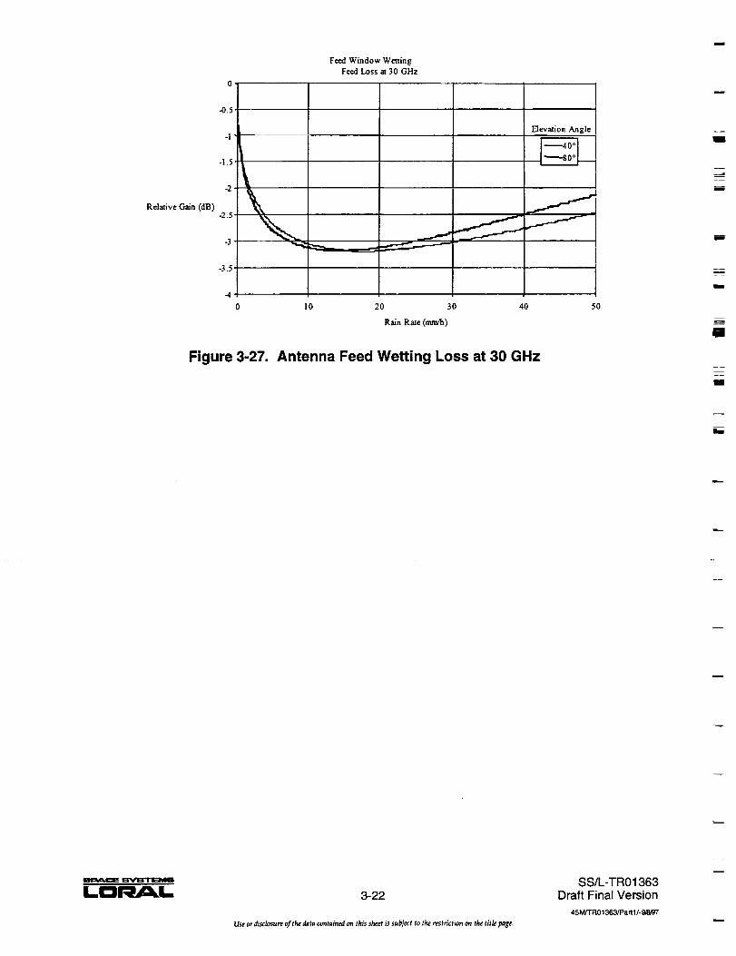
Relative Gain (dB)
0-
-0.5
.| •
-1.5
-2
-2.5
-3
-3.5
-4
0
Feed Window WelxingFeed Loss at 30 GHz
J
He'cation Angle
10 20 30 40 50
Rain Rate(ram/h)
Figure 3-27. Antenna Feed Wetting Loss at 30 GHz
J
m
u
ml
m
=m
i
BE
im
Smp_Lt:E Ept_B'flS_It4_
LC31 L 3-22
Useordisclosure of the datacontainedon thissl_efis subject to the restriction on the title page.
SS/L-TR01363Draft Final Version
45Mr'FRO1363/Part1/-9,_,_7
i

w
SECTION 4 m RAIN FADE MEASUREMENT TECHNIQUES
m.
_,,_._:
°.
w
w
=__
um
m
m
Elinem
Rain fading is a degradation in the power of a signal received at an earth terminal caused
by rain in the propagation path. Fading is typically expressed as a degradation in the
received carrier in decibels. Fading and the accompanying noise temperature increase
caused by rain in the propagation path combine to produce an effective fade, or downlink
degradation. Downlink degradation is an indication of the signal power increase required
to overcome the effects of excess propagation losses and maintain a given link quality.
Since this study is concerned with a comparative evaluation of rain fade measurement and
compensation techniques for two distinct satellite architectures, bent pipe and regenerative
with baseband Switching, fade measurement techniques will be evaluated with respect to
their ability to measure fades at earth terminals caused by rain in the downlink path.
Comparison of fade measurement techniques applied to the measurement of fading caused
by rain on the downlink allows comparisons to be applied to either architecture. Bent pipe
satellite architectures enable the measurement of fades at earth terminals caused by rain in
the uplink path while the regenerative transponder masks uplink impairments from the
remote earth terminals. Also, regenerative satellites can measure uplink fading on-board
the satellite while such techniques are usually not employed on bent-pipe satellites.
Six fade measurement techniques have been evalUated during phase two of this study.
Criteria for comparative evaluation of these six fade measurement techniques include fade
measurement accuracy, speed of response and implementation cost impact on small
terminals. In all cases, accuracy refers to the accuracy of predicting downlink degradation
at earth terminals where the fade measurement equipment resides. Uplink degradation
can be predicted from downlink degradation measurements performed on a common path.
The prediction process involves frequency scaling and the accuracy of uplink
compensation, based on scaled downlink fading estimates, is degraded by the accuracy of
this scaling process. Frequency scaling accuracy affects all fade measurement techniques
equally and is not included in the estimated measurement accuracy. The following sections
cover the six fade measurement techniques. The beacon receiver and modem SNR fade
measurement procedure are _covered in detail while other techniques, which _are Similar in
nature, are covered quickly. Detailed descriptions of the assumptions made in the fade
measurement accuracy analysis for each technique can be found in the appendix.
4.1 ESTIMATING FADE FROM BEACON RECEIVER
Most satellites generate beacon signals which are used as carriers for telemetry data and for
propagation experiments. Beacon signals are typically transmitted in the downlink band
on global coverage horns. Beacon signals can be monitored by the VSAT terminal to
estimate the level of fading on its path. The absolute power of the received beacon signal is
m_
LD_L 4-1
Use or disclosure of the data contained on this sheet is slrbject to the restriction on the title page.
SS/L-TR01363Draft Final Version
45M/FR01363/Part 1/- 9,5,97

compared with a clear-sky reference to determine rain attenuation on the path. A beacon
signal is assumed to be available to all terminals and beacon reception is possible without
antenna feed or LNB modifications. Beacon signals cannot be assumed to be within the IF
band of all terminals though. Terminal equipment must provide beacon receiver circuitry
capable of detecting the beacon within the downlink frequency band at the LNB output.
This circuitry is not otherwise required and therefore increases the production cost of the
VSAT equipment. The beacon receiver circuitry is envisioned to include a synthesizer and
down converter to select the beacon signal from the LNB output, a beacon tracking loop
and circuitry to measure the strength of the acquired beacon signal. Figure 4-1 shows the
basic elements required for beacon signal power monitoring.
The complexity and cost of the beacon receiver is dependent upon the frequency accuracy
of the downconverted beacon signal, the frequency accuracy of the reference provided to
the beacon receiver and the carrier to noise power density of the beacon signal at the
receiver input. The frequency accuracy of the reference and down converted beacon
determine the width of the frequency band over which the beacon tracking PLL must
search to acquire the beacon signal. If this search bandwidth is less than the capture range
of the beacon tracking PLL then a static beacon receiver synthesizer setting will provide
adequate performance and beacon receiver cost will be low. If the search bandwidth
exceeds the capture range of the PLL then a more sophisticated search algorithm is
required. The level of complexity of this algorithm can range from a simple switched filter
approach, where the PLL bandwidth is opened up for signal acquisition then narrowed for
tracking, to more complex processes which involve making repeated signal power
measurements while tuning the synthesizer across the search band and computing the
beacon frequency from symmetry calculations. An example of beacon tracking
performance for the ACTS downlink beacon received by a 1.2 meter VSAT antenna is
provided in section 8.1.1.
m
!
I
= =
mm
mm
i
i
/L-band IF _ Down
(from ODU) --_ Converter
FrequencyReference
(from modem)
I
Synthesizer
Beacon
TrackingPLL
Log
AmplifierBeaconPower
Figure 4-1. Beacon Receiver Block Diagram
LDI'_AE_L 4-2
Use ordisclosureofthedatacontainedon thissheetissubjecttotherestrictionan thetitlepage,
SS/L-TR01363Draft Final Version
45M/TRO 1363tPa rtII-gFJ:J7

w
w
2_
w
z7
w
m
m
w
Beacon signal power measurements are made on a continuous basis by the beacon receiver.
When clear-sky conditions are perceived to exist, beacon power measurements are used to
update a database containing average clear-sky beacon power levels. This database
contains a moving average clear-sky reference beacon level for the current time-of -day
thus enabling the fade estimation algorithm to correct for diurnal variations in received
beacon power. When propagation conditions along the path are determined to be
degraded by rain attenuation, the clear-sky reference level for the current time of day is
divided by the received beacon power level to generate the rain attenuation estimate. A
downlink degradation estimate is determined from the rain attenuation measurement by a
look-up table which assumes a constant system noise and rain media temperatures.
4.1.1 Accuracy- Beacon Receiver
The accuracy of fade estimates generated from beacon signal power measurements is
dependent upon the correlation between rain attenuation and received beacon power,
beacon power measurement accuracy and the effectiveness of the algorithm used to
estimate degradation from beacon power readings. Since received beacon power is the
product of all gain and loss terms in the spacecraft to ground path, variation in any term
will directly affect beacon power level. Table 4-1 shows the sources of fade measurement
error and the residual error which contributes to fade measurement accuracy after time of
day and baseline corrections.
Beacon power readings are an indication of the rain attenuation or fading on the downlink
path. For direct comparison with other fade measurement techniques, the fade
measurement result is used to generate a degradation estimate or effective fade. The
degradation, D/is calculated from the rain attenuation, A, the system noise temperature
under clear-sky conditions, Ts, and the rain temperature, Tm.
L + T.(1- (4-1)
D_A+10 log _r[
Approximations in the above equation include insignificant feed losses, no gaseous attenuation
and constant LNB noise and rain temperature. Errors in the degradation estimate are
aD= ,+
,
(4-2)
Em
LD_k 4-3
Use or disclosure of the data contained on this sheet is subject to the restriction on the title page.
SS/L.-TR01363Draft Final Version
4SM/'FRO 1363/Parl II- 9r-_J7
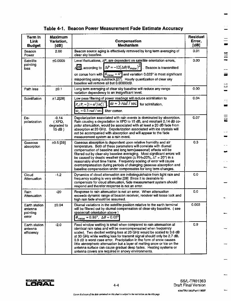
Table 4-1. Beacon Power Measurement Fade Estimate Accuracy
Term in Maximum Residual
Link Variation, Compensation Error,
Budget [dB] Mechanism [dB]
Beacon 2.00 Beacon source aging is effectively removed by long term averaging of 0.01Power clear sky baseline.
_+0.0005 0.00
mw
Satellite
pointingloss
Path loss
Scintillation
De-
polarization
Gaseousabsorption
CloudAttenuation
RainAttenuation
Earth stationantennapointingerror
Earth stationantenna
efficiency
_--_.1
+1.2128]
-0.14( XPD,
degraded to15dB)
_+0.5[28]
-1.2
-2O
_+0.04
-2.0
Level fluctuations, AP Tare dependent on satellite orientation errors,
A[_], according to Z_UP=--I2:AO/O_vmM)2[.Beacon is transmitted
on conus horn with 8_M = 4°1 and variation 0.025 o is most significant
mispointing using autotrack.[27). Hourly quantization of clear skybaseline will remove all but 0.00003dB.
Long term averaging of clear sky baseline will reduce any rangevariation dependency to an insignificant level.
Low pass filtering of power readings will reduce scintillation to
[../.,=(,+o,/o:)']I=--3 for scintillation,
(0o= 0.5 rod / sec filter comer.
Depolarization associated with rain events is dominated by absorption.Rain causing a degradation in XPD to 15 dB, and resultant 0.14 dB co-polar attenuation, would be associated with at least a 20 dB fade fromabsorption at 20 GHz. Depolarization associated with ice crystals willnot be accompanied with absorption and will appear to the fademeasurement system as a rain event.
Gaseous absorption is dependent upon relative humidity and airtemperature. Both of these parameters will correlate with diurnalcompensation of baseline and long term(seasonal) effects will befiltered out by clear-sky baseline averaging. Most significant errors willbe caused by drastic weather changes (4 RH=20%, AT = 20 °) in areasonably short time frame. Frequency scaling of error will causeovercompensation during periods of changing gaseous absorption andbaseline compensation under compensates for long term changes.
Dynamics of cloud attenuation are indistinguishable from light rain andfrequency scaling is very similar.[28] Since it is desirable tocompensate for cloud attenuation, fade measurement system shouldrespond and therefor response is not an error.
Response to rain attenuation is not an error. When attenuationexceeds dynamic range of beacon receiver, receiver will loose lock andhigh rain fade should be assumed.
Diumal variations in the satellite position relative to the earth terminalwill be filtered out by diurnal compensation of clear-sky baseline. ( see
Feed window wetting is small when compared to rain attenuation atidentical rain rates and will be overcompensated when frequencyscaled. Two decibel wetting loss at 20 GHz would be scaled to 3.6 dBat 30 GHz while wetting loss for transmit signal should only be 2.7 dB.0.9 dB is worst case error. Precipitation in the form of snow causeslittle atmospheric attenuation but a layer of melting snow or ice on theantenna surface can cause gradual deep fades. Heating systems orantenna covers are required in snowy environments.
0.00
0.04
0.07
0.3
0.0
0.0
0.003
0.9
m
I
m
w
m
m
I
mi
I
LD_L 4-4
Use ordisclosureofthed_a cont_ned on thissheetissubjecttotherestricfionon thetitlepage.
SS/L-TR01363Draft Final Version
45 M/TR0136&/Pa rt1I- 9r--_97

m
Table 4-1. Beacon Power Measurement Fade Estimate Accuracy (Continued)
= _
Term inLink
Budget
: LNB gain
Beaconreceiver
accuracy
RSSError inattenuation
Averageerror
Accuracy ofdegradationestimate
Maximum
Variation,[dB]
1.0
CompensationMechanism
LNB gain variations with temperature are approximately -0.1 dB/K.Clear-sky baseline will compensate for seasonal changes and diumalcompensation will remove a significant portion of the daily variations.Residual error will be related to worst case day-to-day temperaturechange at constant time of day. (assume 10°C)
Expensive beacon receivers typically have 0.25 dB long term accuracy.Inexpensive circuitry to measure beacon power level should provide0.75 dB long term accuracy without periodic calibration.
All of the above fig.s are worst case errors which can be assumed tobe equivalent to 2LVJ or 95% confidence values.
The mean square error, or lr"_, value is one half of the above result.
Look-up table uses fixed clear-sky system noise and rain mediatemperature and calculates degradation from rain attenuation estimate.(see text )
Residual
Error,
[dB]
1.0
0.75
1.57
0.79
_+1.25dB
. =,
roll=
w
E
m
w
Assumed rain temperature, Tm, is 280+10 K, clear-sky system noise temperature, Ts, is
230+10 K and rain attenuation, A, is 5+0.79 dB. The Beacon Power fade measurement
technique accuracy calculations are summarized for the three satellite architectures in the
appendix, on pages A-1 through A-3. The overall uncertainty in the downlink degradation
estimate is predicted to be +1.25 dB for all three satellite architectures.
4.1.2 Response Time - Beacon Receiver
Logarithmic amplifiers are available which provide the desired accuracy with response
times under I millisecond. When the degradation exceeds the beacon receiver margin, the
beacon receiver will lose lock. Such an occurrence should be interpreted as a extended fade
and the duration of this fade will be prolonged by the beacon receiver acquisition time.
4.1.3 Implementation - Beacon Receiver
The beacon receiver fade measurement technique i s unique in that implementation is
independent of the satellite architecture. The elements included in the blocks shown in
Figure 4-1 are required to measure beacon power and must exist in addition to, and derive
power from, the indoor unit motherboard. Many of the components including the
synthesizer and receiver PLL integrated circuits are available at low cost. Table 4-2 shows a
preliminary estimate of the parts cost for a simple analog beacon receiver with L-band
input.
m
==lI=l, muII! I_f"_l"R
LI31"_D_L 4-5
Use or disclosure of the data contained on this sheet is subject, to the restriction on the title page.
SS/L-TR01363Draft Final Version
45M/TR01363/Patt1/-S_'_J7

Table 4-2. Low Cost Beacon Receiver Parts Cost
Description Manufacturer -Part Number Unit Cost ( Q=1000 )
L-band synthesizer PLL Motorola MC145201 $3.40
L-band mixer TriQuint TQ9172N $4.14
L-band VCO Motorola MC12149 $3.03
IF synthesizer PLL Motorola MC145170 $2.05
Miscellaneous discrete Various Various $5.00
Total = $17
m
mi
u
The beacon receiver must be tested in production and therefore will have a slight cost
impact on the modem arising from increased testing time and the reduction of production
yields. This cost impact, based on a failure rate of 10 -2 and a unit cost of $2K is $20 per
unit. Development costs are estimated to be $120K for the beacon receiver. This cost,
spread over one thousand units will dominate the modem cost impact unless production
quantities are much higher. This fade estimation technique is expected to have a cost
impact of approximately $157 on units produced in quantities of one thousand.
4.2 ESTIMATING FADE FROM MODEM AGC VOLTAGE
Most earth terminal demodulators have variable gain amplifiers which are controlled to
provide constant carrier plus noise (C+N) power at the input to the modem analog to
digital converter. Downlink fading can be estimated from the control voltage of these
automatic gain control (AGC) circuits. This fade measurement technique is similar to the
beacon receiver in that it measures the absolute level of a signal and degradation is
calculated from the measured fade. Fade measurement circuitry samples the modem AGC
voltage at regular intervals and maintains a record of these samples. A fade estimation
algorithm tracks the recent history of AGC voltage measurements and compares them to
the clear-sky baseline for the current time-of-day. The algorithm determines whether
significant fading is being experienced on the downlink path and may factor the current
reading into the clear-sky baseline to follow seasonal variations. The fade estimation
algorithm also estimates the fading from the current AGC voltage reading. This fade
estimate is used to predict the downlink degradation from an assumed system noise and
rain temperature via the same process as described in section 4.1.1 for the beacon receiver
fade measurement technique.
4.2.1 Accuracy - Modem AGC Voltage
The accuracy of degradation estimates based upon modem AGC voltages are dependent on
the satellite architecture and satellite performance as well as the AGC voltage measurement
and fade estimation process. The received C+N power level accuracy calculations are
summarized in Appendix A, on pages A-4 through A-6, for each satellite architecture. A
backed-off bent pipe satellite will exhibit uplink power variations which, when combined
m
i
= =
BB
=_
m
u
gim, A_! lS'V'IFI'I_IB
4-6
Use ordisclosure of thedata contained on this sheetis subject to the restrictionon the title page.
SS/L-TR01363Draft Final Version
45M/TR01363/Pa rtI i-9,5/97

m
=_
w
=_
with satellite gain variations and downlink variations similar to the beacon power
measuremenL will affect tl_e downlink:carrier power. The combined effect of these
uncertainties is a 1.14 dB uncertainty in the received carrier power. A saturated
transponder and the on-board processing satellite will limit these variations and provide
improved uncertainty of 0.66 dB and 0.65 dB respectively for the received carrier power.
For satellite links operating with concatenated coding and with clear-sky link margins of
4 dB, the relationship between C+N power and fading can be approximated by Equation
(4-3) which is shown in Figure 4-2 below.
1.00
0.90
0.80
0.70
_0.60
U
_ 0.50
0N
= 0.40
_ 0.30
0.20
0.I0
(C/N)cs =9 dB
Tm = 280 K
Ts = 240 K
3 (C+N) = 1.5 dB
0.00
0 1 2 3 4 5 6 7 8 9 10
Rainattenuation,A, [dB]
Figure 4-2. Effect of Carrier plu s Noise Power Uncertainty on Estimated Fade
I(C+N)'r=(C+N)¢_-A+IOI°g " T_ "
( C + N). = clear sky carrier plus noise power
( C + N) I = faded carrier plus noise power
A, T m, & T, as previously defined.
(4-3)
w
LD L 4-7
Use or disclosure of the data contained on this sheet is subject |o the restriction on the title page.
SS/L-TR01363Draft Final Version
45M/TR01363/Paa1/-9r-J97
Received carrier plus noise power uncertainty of 1.14 dB creates a relatively large +1.75 dB
uncertainty in the estimated attenuation. This attenuation estimate is used to estimate
downlink degradation and results in a degradation uncertainty of 3.94 dB. This
uncertainty is much higher than those provided by the other 5 fade measurement
techniques and eliminates this fade measurement technique from further investigation.
4.2.2 Response Time - Modem AGC Voltage
The modem AGC fade measurement technique can provide fade estimates whenever the
modem demodulator is tuned to a received carrier. Fade estimates can be read from the
demodulator circuitry at an arbitrarily high rate limited by the processing requirements of
the fade estimation algorithm. The bandwidth of the AGC control loop is typically 0.01 to
0.001 times the modem symbol rate as it is undesirable for the AGC circuitry to respond to
instantaneous fluctuations in the received carrier and noise power. For a QPSK modem
passing an information rate of 384 kb/s, with concatenated coding and reasonable framing
overhead, the symbol rate will be around 300 ksymbols/s. A typical AGC loop bandwidth
would be around 1.5 kHz and the AGC voltage will follow any propagation phenomena
with delays less than 10 ms.
4.2.3 Implementation - Modem AGC Voltage
Implementation of the modem AGC fade measurement technique has very low impact on
modem complexity and a possible slight impact on modem parts cost. Demodulators have
AGC loops in place and only an additional processor function is required to read and
record the modem AGC voltage. If the AGC loop is implemented digitally then no
additional parts are required. If the modem AGC loop is analog then an A/D converter
may be required to measure the analog control voltage if one is not already available in the
modem. A suitable, low speed converter and associated circuitry would cost approximately
$10 in quantities of one thousand. Any additional features must be tested in production
and therefore will have a slight cost impact on the modem arising from increased testing
time and the reduction of production yields. This cost impact, based on a failure rate of
10 -3 and a unit cost of $2K is $2 per unit. Development costs are estimated to be $80K for
the fade measurement circuitry. This cost, spread over one thousand units will dominate
the modem cost impact unless production quantities are much higher. The total modem
cost impact for the modem AGC fade measurement circuitry is estimated to be $92.
4.3 ESTIMATING FADE FROM PSEUDO-BIT ERROR RATE
Downlink degradation can be estimated directly from measurements of channel
performance parameters which depend upon Es/No compared with similar measurements
performed under clear-sky conditions. The Pseudo BER fade measurement technique is the
first of four techniques of this type[29]. A secondary demodulator path is created and this
path is intentionally degraded by establishing restricted decision thresholds. In a link
W
=
m
I
W
=_.._
m
E
--=
r_
w
w
lSlIqAI_IE
4-8
Use or disclosure of the data contained on this sheet is su_cct to the restriction on the title page.
SS/L-TR01363Draft Final Version
45M/TR01363/Partl/-_oB7

w
L
w
employing QPSK modulation a pseudo-error region would count as error those symbols
whose phase fell into the shaded region of Figure 4-3 while the primary channel would
continue to use the orthogonal axes as decision thresholds to yield the lowest BER.
The relationship between channel BER and pseudo-BER varies little over a wide range of
channel conditions. Pseudo-error zone width may be selected to trade accuracy for
measurement speed so that a pseudo-error measurement may be completed much more
quickly than an actual BER measurement of identical accuracy.
4.3.1 Accuracy - Pseudo Bit Error Rate
The Pseudo-BER fade measurement technique, like all techniques which measure fades
from Eb/No, is insensitive to VSAT terminal LNB gain variations. LNB gain variations
affect noise power and signal power equally and therefore do not change Eb/No. There
are still uncertainties in the received Eb/No that are not related to rain attenuation. These
uncertainties are summarized in Appendix A, on pages A-7 through A-9, for the three
satellite architectures. Assuming the measurement interval is selected to provide a degree
of confidence of 0.25 on the Pseudo-BER measurement, then the degree of confidence in the
actual BER is increased by the magnitude of the slope of the log(Pe) versus log(Pp) curve
shown in Figure 4-5. This slope is -1.63 resulting in a degree of confidence of 0.41 for the
BER measurement. This 41% range of BER values about average value of 0.01 translates to
an uncertainty in the Eb/No value of +0.5 dB (see Figure 4-4). The overall uncertainty in
the downlink degradation estimate is predicted to be 1.06 dB for the backed-off bent pipe
satellite and +0.50 dB for the other two satellite architectures.
q
===
w
O O
Figure 4-3. Shifted-Phase Decision Thresholds for
Pseudo BER Fade Measurement
LDI'_/_I.. 4-9
Use or disclosure of thedata containedon this sheet is subject to therestrictionon the title page.
SS/L-TR01363Draft Final Version
45MrI'R01363_art 1I-9F_97

1.00E+00
1.00E-01
1.00E-02
mm1.00E-03m
1.00E..04
1.00E-05
1.00E-06.. :, ,,. ,* .... ! .... ! .... !, , -, .... • .... ! .... _ ....
0 1 2 3 4 5 6 7 8 9 10
Eb/No, (dB)
mi
n
m
g
IB
i
Figure 4-4. Theoretical BER Performance of QPSK Signal
on Ideal Linear Channel
BER
BBI
_ I
w
Figure 4-5. Pseudo BER Versus Actual BER on
Ideal Linear Channel
Btm__
4-10
Use or disclosl_re of the data contained on this she_ is subject to the restriction on the tit/e pa_e.
SS/L-TR01363Draft Final Version
45 M/TR01363,,'Pa rt 1/- _/8,97

k_.
1
w
mw
4.3.2 Response Time - Pseudo Bit Error Rate
The required degree of confidence in the measurement of Pseudo-BER, Pc, can be obtained
by measuring over an observation interval of n=6.2x10³ symbols. For the channel rates
encountered carrying a 384 kb/s information rate the QPSK symbol rate is approximately
300 ksymbol/s which results in an observation interval of 21 ms.
n- p_pp (4-4)
K¢ = Number of standard errors of the mean
= 1.96 for 95% confidence level
Pc = Required confidence in Pseudo - BER measurement
= 0.25
Pp = Pseudo- BER
= 0.01.
4.3.3 Implementation - Pseudo Bit Error Rate
The Pseudo-BER fade measurement technique is another technique which only provides
useful measurements while the demodulator is locked to the desired carrier. Pseudo-BER
measurements performed to estimate downlink degradation require additional circuitry to
generate a pseudo-error count over the desired measurement interval. This fade
measurement process can be implemented with four comparators operating at the channel
symbol rate, four latches to sample the comparator outputs at the appropriate instant, a
four input exclusive-or gate and a counter. Total parts cost is estimated to be less than $5.
This circuitry should generate less than 10 -3 production test failures per unit which, for a
unit production cost of $2K, results in a cost impact of $2 per unit. Development cost for
the fade measurement circuitry are estimated to be less than $50K resulting in a cost impact
of $50 per unit for total production of 1,000 units. The sum of these cost factors is $57 per
unit.
4.4 ESTIMATING FADE FROM BER ON CHANNEL CODED DATA
On systems which utilize forward error correction, measurements of channel bit error rate
(BER) within the modem can be used to estimate path loss due to rain attenuation. As
fading occurs the carrier to noise power ratio degrades and the decoder correction rate
increases. Channel bit error rate is measured by re-encoding the decoded channel data and
comparing the re-encoded data with a delayed version of the original channel data. Any
discrepancies are corrections performed by the decoder. These corrections are counted and
divided by the bit count to determine the channel BER.
t-D_L 4-11
List or disclosure of tim data contained on this sh_ is subj_t to the r_striction on the title page.
SS/L-TR01363Draft Final Version
45M/TR01363/Pa_1/-9/5/g7

4.4.1 Accuracy - BER from Channel Coded Data
The accuracy of fade estimates generated from channel BER measurements is dependent
upon the correlation between fading and channel BER and channel BER measurement
accuracy. Effects which decouple downlink C/N and rain attenuation can include uplink
compensation errors, satellite gain variations, antenna gain and antenna pointing errors.
Efforts to filter out these sources of error will never be completely effective and residual
errors will contribute to fade measurement uncertainty. Appendix A, on pages A-10
through A-12 shows the principle sources of signal to noise ratio variations and estimates
of the mean square error in the Eb/No ratio. This error, combined with the error in
measuring channel BER, combine to reduce the accuracy of fade estimates. The overall
uncertainty in the downlink degradation estimate is predicted to be +1.04 dB for the
backed-off bent pipe satellite and _+0.46 dB and +0.45 dB for the saturated bent pipe and on-
board processing satellites respectively.
4.4.2 Response Time - BER from Channel Coded Data
Assuming channel BER is measured on a 384 kb/s carrier the above accuracy can be
obtained in less than 17 milliseconds. For lower baseband data rates more time would be
required to accumulate statistics. On high rate data streams, such as a 90Mb/s TDM
stream the response time is significantly lower.
4.4.3 Implementation - BER from Channel Coded Data
This technique can be utilized independent of satellite access schemes because it operates
on the recovered data. If FEC is not utilized a similar technique can be implemented by
measuring the BER of a known sequence such as the unique word in a TDMA system or
framing bits in a TDM system. In this case response times will be much longer due to the
limited number of bits for error measurement. All forms of this fade estimation technique
can also be implemented on the satellite.
Circuitry required to implement this fade estimation technique include the re-encode
circuitry, a comparator, a channel error counter, a channel bit counter and a processor to
estimate the fade from the channel BER measurement. For data rates below 25 Mb/s
integrated circuits are available for convolutional encoding and Viterbi decoding. These
devices, which presumably already reside within the modem, have built-in re-encode
circuitry, a comparator, a channel error counter and a channel bit counter. There is
therefore no additional parts cost associated with this fade measurement technique. This
circuitry should generate less than 10 -3 production test failures per unit which, for a unit
production cost of $2K, results in a cost impact of $2 per unit. Development cost for the
fade measurement circuitry is estimated to be less than $50K resulting in a cost impact of
$50 per unit for total production of 1,000 units. The sum of these cost factors is $52 per
unit.
imm
i
R
W
i
: :
w
ll=l, alj_m
I.,DI'_U_L- 4-12
Use or disclosuw of the data contained on this sheet is subject to the restriction on the title page.
SS/L-TRO 1363Draft Final Version
45M/TR01363/Part 1/- 9FJ97
w
!
m
m_
w
M
m
m
For higher rate systems, all of the circuitry to measure channel BER and compute fades
impacts terminal cost. The re-encode circuitry, compare circuitry, bit counters and error
counters are relatively simple when compared with the task of decoding the encoded data.
The additional circuitry to accumulate BER statistics would have minor incremental cost
impact. A microprocessor is still required to complete the fade estimation circuitry and
implement the compensation algorithm. The terminal cost impact of this fade estimation
technique for bit rates above 25 Mb/s data is approximately $50.
4.5 ESTIMATING FADE FROM BER ON KNOWN DATA PATTERN
Virtually every satellite communication channel carries some overhead bits to indicate
multiplexing frame boundaries, provide carrier phase reference, provide carrier frequency
reference or burst time references to receiving terminals. These overhead bits typically
constitute 3% to 5% of the channel capacity. BER measurements can easily be performed
on these bits because the receiving terminal has a-priori knowledge of their content. Fade
estimates can then be based on the results of these measurements.
4.5.1 Accuracy - BER from Known Data Pattem
BER measurements performed on known data patterns are measurements of channel
quality and do not rely on the absolute accuracy of any power level measurement. This
technique for estimating fading is therefore immune to LNB gain variations and the
uncertainty in the received signal quality is similar to the BER from channel coded data,
SNR and pseudo-BER measurements. Assume that the known data pattern is not encoded
and the channel is operating at a BER of 0.01 corresponding to a BER of 3x10 -4 after the
Viterbi decoder and quasi-error free (10 -10 - 10 -11) after the Reed-Solomon decoder. A 40%
tolerance on measuring the BER indicates that the 95% confidence interval for measured
BER is 0.01 + 40% or 0.006 < BER < 0.014. Reading from the un-coded QPSK curve of
Figure 4-4 yields an uncertainty in Eb ]NO of +0.5 dK This uncertainty is combined with
additional uncertainties associated with the upi_ and downlink uncertainties in Eb/No in
Appendix A, on pages A-13 through A-15. The error in the degradation estimate is
+1.06 dB for the saturated bent-pipe, _+0.50 dB for the backed off bent-pipe and +0.49 dB for
the on-board processing satellite.
4.5.2 Response Time - BER from Known Data Pattern
Since the BER measurement is performed on only a small fraction of the channel bits, more
measurement time is required to provid_e acceptable accuracy. To achieve the 40%
tolerance on measured BER for a 384 kbit/s stream requires a 1,200 bit measurement
interval or 0.10 seconds for a 3% known pa_ern content.
B
w
4-13
Use or diaclosure o/the data contained ca this sheet is subject to the restriction on the title page.
SS/L-TR01363Draft Final Version
45M/TR01363/Part 1/- _lr-J_'

4.5.3 Implementation - BER from KnownData Pattern
This fade measurement technique can only provide meaningful degradation estimates
when the demodulator is locked to the desired data stream. The demodulator will not
have the advantage of knowing the current degradation during the link acquisition
procedure. This fade measurement technique does not add any additional parts to the
modem. Any known data pattern in the aggregate stream is monitored on a continuous
basis by the modem to either provide or verify proper operation of the communication link.
The cost associated with this technique is only that associated with the expense of
developing a process to accumulate the BER statistics and can be assumed equal to the BER
from Channel Coded Data fade measurement technique.
4.6 ESTIMATING FADE FROM SIGNAL TO NOISE RATIO
Measurements of signal power to noise power ratio (SNR) within the modem can also be
used to estimate path loss due to rain attenuation. As fading occurs the carrier to noise
power ratio degrades according to the following formula.
+ A (4-5)C� Ndegredation in decibles = 10log T,
T, = System noise temperature under clear sky conditions
A = Rain attenuation in decibels
T m = Rain temperature
The first term accounts for the increase in system noise power caused by rain absorption
and the second term accounts for the signal attenuation. The above relationship is plotted
for several system clear sky noise temperatures in Figure 4-6. The effective fade, or
degradation, is approximately 1.5 times higher than the rain induced attenuation.
=_en=this technique is implemented on the satellite, the scaling between rain attenuation
and SNR degradation is one because the noise temperature "seen" by the satellite is always
high, essentially equal to the earth surface temperature.
Within the modem the baseband signal to noise ratio can be calculated from data samples.
If we assume QPSK data with no inter symbol interference the signal to noise ratio is
(DIl+le)SNR -
22(1 = + Q=)_(ZItI+IQI)Z (4-6)
22 G
wi
lib
R
N
Ill
m
_Iu
l
w
w
w
w
LCI_L 4-14
USe or disclosure of tke data contained on this sheet is subject to tht restriction on the title page.
SS/L-TR01363DraftFTna[Version
45M/TR013631Part1I-9,5,97
w
u

=
w
,=:
E=
Z
w
m
: =
°--
3O
25
0
0 2 4 6 8 10 12 14 16 18 20
Rain Attenuation, A (dB)
:----_- lOO i_---I1_ 150 i
--&--20o !_._K._25O ,Z--_ looooooI
Figure 4-6. C/N Fading Caused by Rain Attenuation
Where I and Q are the I-channel and Q-channel data samples. Fade estimates are
calculated from the signal to noise measurement and assumptions on the receiver noise
temperature from the above graph.
4.6.1 Accuracy - Signal to Noise Ratio
The accuracy of fade estimates generated from signal to noise power measurements is
dependent upon the correlation between fading and signal to noise ratio and signal to noise
measurement accuracy. Effects which can decouple downlink Eb/No and rain attenuation
include uplink compensation errors, satellite gain variations, antenna gain and antenna
pointing errors. Efforts to filter out these sources of error will never be completely effective
and residual errors will contribute to fade measurement uncertainty. These uncertainties
are summarized in the appendix, on pages A-16 through A-18, for the three satellite
architectures. The overall uncertainty in the downlink degradation estimate is predicted to
be 1.03 dB for the backed-off bent pipe satellite, +0.43 dB for the saturated bent pipe and
+0.42 dB for the on-board processing satellite architecture.
4.6.2 Response Time - Signal to Noise Ratio
Assuming Signal to Noise is measured on a 384 kb/s carrier the above accuracy can be
obtained in less than 10 milliseconds. For lower baseband data rates more time would be
required to accumulate statistics. On high rate data streams, such as a 90 Mb/s TDM
m
m
I3"Y'EFr_
LC3RM_L 4-15
Use or disclosure of the data contained on this sheet is subject to the restriction on the title page.
SS/L-TR01363Draft Final Version
45M/'FR01363/Par111-9_/97

stream the response time trades with implementation cost. In this case response times
below 10 milliseconds can be obtained at low costs.
4.6.3 Implementation - Signal to Noise Ratio
This technique can be utilized independent of satellite access schemes because it operates
on the baseband signal. This fade estimation technique can also be implemented on the
satellite.
_z
I
I
Figure 4-7 shows a hardware implementation which can function in TDMA and high rate
TDM environments. This implementation takes advantage of the fact that SNR readings
are required only a few times per second. The First-In-First-Out (FI_O) memories are the
only element which must function at the channel symbol rate. A sufficient number of
successive data samples are read into the FIFO to obtain the required SNR accuracy. A
microprocessor then processes the data by accumulating the required summations,
calculates the SNR and implements the fade compensation algorithm. A programmable
logic device is included to control the FIFO loading and perform other ancillary functions
which may be required to interface with the modem. The terminal cost impact of this
I
i
m
i
i
I-channel
D/A
Baseband __
Quadrature _ Signa_Demodulato_--] ,
Q-channelD/A
Data Samples
Programmable ILogic
Device [
II-channel
FIFO
I
IQ-channe_
FIFO |
II
_{ Processor tMemo_
Figure 4-7. Signal to Noise Ratio Measurement Hardware
Demodulator
_I
m
==
= =
w
LD_L 4-16
Use or disclosure of the data contained on this sheet is subject to the restriction on the title page.
SS/L-TR01363Draft Final Version
45M/TRo 1363/Part 1/-9FJ,97
w
w

=
w
=--
circuitry is estimated to be approximately $12 for a low speed FIFO memory integrated
circuit. The processing and data handling burden is assumed to be incorporated into the
modem with no parts requirement. The cost associated with reduced production yields
due to a 10 -3 test failure rate for the fade measurement circuitry is $2 for unit costs of $2K.
Fade measurement circuitry development cost is estimated to be $80K which adds $80 to
the per unit cost for production quantities of 1000 units. The combined cost impact of this
fade measurement technique is estimated to be $94.
4.7 SUMMARY OF FADE MEASUREMENT TECHNIQUES
The six fade measurement techniques are summarized in Table 4-3. Three techniques were
selected for further investigation as indicated. The beacon power measurement technique
was selected because its performance is independent of satellite architecture and the cost
factor will improve with higher production volumes. The Modem AGC technique was
excluded based upon poor predicted accuracy. The Pseudo-BER, BER from Channel
Coded Data and BER from Known Data Pattern technique are very similar in performance.
BER from channel coded data was selected to represent this group because channel coding
will most certainly be employed and many modems are available with this feature. The
SNR technique was also included based upon low cost impact and good accuracy.
Technique
Satellite Beacon
Modem AGCLevel
Table 4-3. Summary of Fade Measurement Techniques
Accuracy of Degradation Estimate
Cost to Speed of Bent Pipe/ Bent Pipe/ On-boardImplement Response Backoff Saturated* Processing
$157 0.001 sec
0.01 sec
1.25
3.94
1.25
2.17
1.25
2.17$92
Pseudo BER $57 0.02 sec 1.06 0.50 0.50
$52 0.10 sec 1.06 0.50 0.49Channel BERfrom a KnownData Pattern
0.02 sec 0.46$52BER Monitoringfrom ChannelCoded Data
0.451.04
Modem Signal to $94 0.01 sec 1.03 0.43 0.42Noise Ratio
* Assumes that overdrive is maintained through all uplink fades. Otherwise bent-pipe withaccuracy is more appropriate.
Selected forExperiment
v"
v"
,/
pack-off
=_
mw
z
4-17
Use or disclosure _ th¢ data contained an this sheet is subject to tht restriction an the title page.
SS/L-TR01363Draft Final Version
45M/FR01363/Part 1/-_5/g7

i
a_
i
i
: =
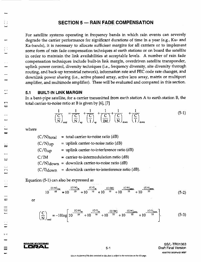
=
w
--J
==:
SECTION S -- RAIN FADE COMPENSATION
For satellite systems operating in frequency bands in which rain events can severely
degrade the carrier performance for significant durations of time in a year (e.g., Ku- and
Ka-bands), it is necessary to allocate sufficient margins for all carriers or to implement
some form of rain fade compensation techniques at earth stations or on board the satellite
in order to maintain the link availabilities at acceptable levels. A number of rain fade
compensation techniques include built-in link margin, overdriven satellite transponder,
uplink power control, diversity techniques (i.e., frequency diversity, site diversity through
routing, and back-up terrestrial network), information rate and FEC code rate changes, and
downlink power sharing (i.e., active phased array, active lens array, matrix or multiport
amplifier, and multimode amplifier). These will be evaluated and compared in this section.
5.1 BUILT-IN LINK MARGIN
In a bent-pipe satellite, for a carrier transmitted from earth station A to earth station B, the
total carrier-to-noise ratio at B is given by [6], [7]
1 1 1 I 1 1
where
c = C + C
(C/N)total =
(C/N)up =
(C/I)up =
C/IM =
(C/N)down =
(C/I)down =
total carrier-to-noise ratio (dB)
uplink carrier-to-noise ratio (dB)
uplink carrier-to-interference ratio (dB)
carrier-to-intermodulation ratio (dB)
downlink carrier-to-noise ratio (dB)
d0wnlink carrier-to-interference ratio (dB).
(5-1)
Equation (5-1) can also be expressed as
(C/N)wt. , (C/N)u p (Cll)_
10 io =10 lo +10 1o +10
or
(C/IM) (C/N)ao, _ _(C/I),_,,=
_o +10 _o +10 _o (5-2)
(C) =-101og[10 (cm), (cn)o_ (C,_M)+10 F6 +10 i_ +10
total
_o + 10
(C/l)d,,_
I0
.
(5-3)
w
EDgE 5-1
Use or disclosure of the data contained on this sheet is subject to the restriction on the title page.
SS/L-TR01363Draft Final Version
45MfI"R01363/Part2/- 9,_,_/
As seen from Equation (5-3), if one of the five ratios becomes much smaller than the others,
the total carrier-to-noise ratio is almost equal to this ratio. In this case, it is often termed
that the link is limited by this component. In operational satellite systems, depending on a
number of factors such as service requirements in terms of carrier bit rate, modulation and
coding, required BER performance, and link availability; earth station antenna diameter
and high-power amplifier (HPA) size; climate conditions at earth stations; satellite
parameters (e.g., saturation flux density, EIRP, and G/T); and interference environment,
the total carrier-to-noise ratio can be limited by more than one component.
In general, a link or system margin is allocated to a link in order to provide a specified link
availability. A high system margin is required for a high link availability. In a bent-pipe
transponder, the transponder capacity is a function of the system margin: the higher the
margin the lower the capacity. As seen from Equation (5-3), this nonlinear function
depends on the factors mentioned earlier. In a system in which carriers are allocated
margins to provide a threshold BER performance at a specified link availability, the carrier
BER performance is, under clear-sky conditions, much better than the threshold BER
performance. Since these margins are permanently assigned, the capacity is fixed.
Therefore, it is not possible to achieve an increase in the capacity which could have been
realized had the fixed margins not been allocated or had smaller fixed margins been
allocated and additional margins provided by earth stations and/or spacecraft on an
adaptive basis during periods of severe rain fades.
It should be noted that, in a multicarrier-per-transponder operation, the total transponder
input backoff is normally set in the quasi-linear region in order to minimize the IM
impairment. Consequently, the individual carrier input backoff is set in the linear region.
The uplink margin is normally equal to the system margin since an uplink fade would
affect almost equally the (C/N)up, (C/I)up, C/IM, (C/N)down, and (C/I)down. For a
downlink fade, the downlink margin is normally much larger than the system margin since
only the last two components are affected. As an example, for the IDR (intermediate data
rate) service offered in the Ku-band in the INTELSAT system, the nominal uplink margin
and downiink margin are equal to 7 dB and 11 dB, respectively [30]. In a single-carrier-per-
transponder operation, the total transponder input backoff is normally set in the saturation
region since there is no IM impairment. (Here, nonlinear distortions due to TWTA or SSPA
nonlinearities become dominant [31].) The uplink margin is normally larger than the
system margin since an uplink fade would not affect equally the (C/N)up, (C/I)up,
(C/N)down, and (C/I)down. For a downlink fade, the downlink margin is normally much
larger than the system margin since only the last two components are affected.
w
=_
i
i
i
i
U
w
LD__ 5-2
Id_ or disclosure of the data contained on this sheet is s_lb_ect to the restrictic,n on the title page.
SS/L-TR01363Draft Final Version
45 M/TRO 1363/Pa rt2/- _r--r'_7

r
W
"mU
m
In an OBP satellite, for a carrier transmitted from earth station A to earth station B, the
information BER performance at B, BERi, is given by [13]
BERi = BERiu + BERid (5-4)
where
BERiu = uplink information BER
BERid = downlink information BER.
BERiu is a function of (C/N)up and (C/I)up, BERid a function of (C/N)down and
(C/I)down. It is worth noting here that uplink noise and interference components, and
downlink noise and interference components do not accumulate or add up like those
shown in Equation (5-3). In a special situation in which Cup/(Nup+Iup), the ratio of uplink
carrier power to uplink thermal noise and interference, is equal tO Cdown/(Ndown+Idown),
the ratio of downlink carrier power to downlink thermal noise and interference, close to
3-dB advantage in system margin can be realized as compared to a similar situation using a
bent-pipe satellite. In a link, the uplink or downlink margin is always larger than the
system margin. From Equation (5-4), the allocation of a fixed uplink margin can be
performed independently from the allocation of a fixed downlink margin, depending on
climate conditions at the transmit and receive earth stations. For a large downlink TDM
carrier, the allocation of a large fixed downlink margin may reduce the carrier information
rate.
Therefore, while the built-in link margin technique is simple, and can reduce the
complexity and cost associated with a network, the requirement of large fixed margins in
the Ka-band (much larger than margins required in the Ku-band) will adversely affect the
system capacity in bent-pipe and OBP satellites.
5.2 OVERDRIVEN SATELLITE TRANSPONDER
In a bent-pipe satellite, in order to minimize the effects due to high uplink rain fades, it is
possible, in a single-carrier-per-transponder operation, to transmit a high-power carrier
from an earth station such that the transponder TWTA operating point is set well into the
overdrive region (i.e., 4 dB or more beyond saturation) as shown in Figure 5-1. For
example, in the Ku-band, a 7-dB fade in the uplink will reduce the TWTA operating point
from +4 dB to -3 dB. The corresponding reduction in downlink carrier EIRP is small (e.g.,
about 0.5 dB for a TWTA [18]). Therefore, by operating the TWTA in the overdrive region,
high uplink fades can be tolerated while keeping the downlink carrier EIRP at about the
same level. Consequently, the degradation due to an uplink fade on the carrier BER
w
mm
5-3
Use or disclosure of the data contained on this sheet is subject to the restriction on the title page.
SS/L-TR01363Draft Final Version
45 M/'rR01363JPatt2/- _,97

Saturation
Quasi-Linear
Region
Linear _Region
/
Overdrive
Region
_ TWI'A Operating== PointO
o
(._
:3O
Input Backoff (dB)
Figure 5-1. Transponder TWTA Operation in Overdrive Region
performance is almost negligible. (It has been implicitly assumed here that the link is not
limited in the uplink. This is normally the case in single-carrier-per-transponder
operations.)
This technique is only suitable for systems in which a single high-power carrier is
transmitted through a single transponder TWTA whose operating point is set beyond
saturation. Here, the nonlinear effects [32], [31] due to the TWTA on the carrier
performance (i.e., BER performance, power spectrum re-growth, etc.) must be fully
evaluated and accounted for in the system design and associated link budgets. This
technique is not useful in commercial multicarrier operations with FDMA or code-division
multiple access (CDMA) carriers due to severe IM impairments.
5.3 UPLINK POWER CONTROL
Uplink power control is a technique in which the carrier uplink EIRP is adjusted on an
adaptive basis based on the continuous measurement, in the downlink, of the power of
another carrier or of the same carrier. The amount of uplink power adjustment is estimated
from this measured downlink fade. Depending on the satellite beam configurations (i.e.,
connectivities and coverages) and availability of beacons, and the earth station locations in
the beam coverages, this technique can be implemented in three different ways: open-loop,
closed-loop, and feedback-loop.
In an open-loop system (e.g., in a non-loopback beam), an earth station cannot receive its
own transmit carrier, and needs to rely on a measurement of the downlink beacon fade. In
a closed-loop system (e.g., in a global beam or loopback beam), an earth s_tation can receive
its own transmit carrier as well as carriers from other earth stations with which it is
communicating. It is preferable to estimate the uplink power adjustment based on the
I
m
m
w
g
i
:_u
=
LD L 5-4
Useordisclosure of thedata containedon this sheet is subject to therestriction on the titlepage.
SS/L-TR01363Draft Final Version
45M/rR01363/Part2/- 9Fa97
--4 •
B
w
=
==_
w
fade measurement of one of these carriers instead of the same carrier since the
measurement of the latter is not accurate due to variations in carrier input backoff and
associated variations in carrier output backoff under upiink and downlink fadings (i.e., rain
at an earth station affecting simultaneously the carrier being transmitted and received). In
a feedback-loop system (e.g., in an east-to-west beam and a west-to-east beam), a central
control station monitors the powers of all carriers it receives in one beam, and commands,
through the other beam, earth stations which undergo uplink fadings to adjust their uplink
EIRP's. It is implicitly assumed here that rain does not occur simultaneously in the two
beams. Among the three systems, the last one requires more space segment and ground
segment resources than the first two. In addition, an earth station which undergoes uplink
fadings has to wait at least two round-trip propagation delays before it can receive
instructions from the central control station to increase its uplink carrier EIRP.
In a bent-pipe satellite, any one of the three selected rain fade measurement techniques (i.e.,
beacon power, bit error ratio from channel coded data, and signal-to-noise ratio) can be
used to estimate the uplink power adjustments. In an OBP satellite, one of the last two
techniques can be used on board the satellite to measure the uplink powers of all carriers.
Appropriate commands can then be sent, in the downlink, to the affected earth stations to
adjust their uplink carrier powers accordingly.
An experiment was conducted by COMSAT Laboratories at Clarksburg, Maryland using
ACTS during the May - November 1994 to evaluate the feasibility of the open-loop uplink
power control technique [28]. It was found that, under most conditions, a power control
accuracy of +2.5 dB could be maintained and uplink fades of up to 15 dB could be
compensated. A summary of key ACTS experiments was described in [33].
5.4 DIVERSITY TECHNIQUES
Over the years various diversity techniques have been proposed for mitigating rain fading
at frequencies above about 10 GHz. These include frequency diversity, site diversity,
terrestrial backup, and orbital diversity. Some of these techniques are briefly discussed
below.
5.4.1 Frequency Diversity
Rain attenuation, expressed in dB, increases with the frequency approximately in
proportion to the square of the frequency. Rain attenuation at 20 GHz is almost three times
that at 11 GHz. Figure 5-2 shows therain attenuation distributions at 4, 6, 11, 14, 20, and 30
GHz for a mid-Atlantic location; elevation angle is 40 °. Although frequency diversity can
be used to mitigate rain fading at Ka-band frequencies, the requirement of complex feed
systems or separate antennas may out weigh any advantage offered by this technique.
mP.A.Iml _sYECll-r==_9
LDI=_dI_L 5-5
Use or disclosure of the data contained on this sheet is subject to the restriction on the title page.
SS/L-TR01363Draft Final Version
45 M/TR 01363,'Pa rt2/. 9,_J7

50
40 '_
30'
Attenuation
(dB) 20 )
101
|
0
0.01
I{}ll{[I{ll}l{Irl {{I}{{l{l{{lll{lIll{ [l{11
{11{1{IIII {1{111Ililll{{{{I{I}ll
. I llll0.1 1 10 100
Percent Time Ordinate Exceeded
!_6 GHz ]
•"i-- 11GHz I
14 GHz I
_20 GHz I_30GHz I
Figure 5-2. Cumulative Distribution of Rain Attenuation at Different
Frequencies for a Mid-Atlantic Location; Elevation Angle 40 °
mum
r_
IBB
==mw
I
5.4.2 Site Diversity
The limited horizontal extent of rain storms, and the non-uniformity of rain intensity
within a storm are exploited in site diversity. In the presence of severe rain fading site-
diversity has a significant advantage in improving link availability. Site diversity
experiments on earth-space paths with elevation angles above about 20 ° have shown that
diversity improvement increases rapidly as the site separation approaches, and exceeds,
about 10 km, saturating beyond about 20 kin. For elevation angles below 20 °, the site
separation requirements appear to increase proportionately. Diversity applied in the
conventional sense requires two dedicated earth stations to support a single satellite link.
In general, the cost involved in setting up the two earth stations and connecting them
together appears to outweigh the benefits rendered.
Finite size of rain cells results in uncorrelated fading at sites separated by distances larger
than the average rain cell size. In general, the average cell size is inversely proportional to
the rain intensity and diversity can be highly effective in combating relatively strong fades.
Improvement in link availability with the use of diversity is normally quantified as
diversity gain or diversity advantage. Diversity gain is the difference between the single
site attenuation and the joint attenuation between the two sites, both taken at the same
probability level. The diversity gain may be predicted using the model recommended by
the ITU-R [17]which requires frequency, site separation, elevation angle, and the base line
orientation angle as the input parameters; the baseline orientation is the angle between
the line joining the two sites and the projection of the radio path on the earth surface.
Figure 5-3 and 5-4 show the predicted diversity gain at 20 and 30 GHz, respectively, as a
function of single site attenuation. At the low end of the single site attenuation very little
U
hil
N_
5-6
Use or disclosure of the data contained on this sheet is subject to the restriction on the title page.
SS/L-TRO 1363Draft Final Version
45 M/TR01363/Pa rt?J- 9_/97w

z
r
16
14
12
io
8
.9e_
DiversityGain at 20 GHz
-,¢__jr-- ;ite Separation
0
0 5 10 i5 20 25 30
Single Site Attenuation (dB)
s..,..
L_
Figure 5-3. Diversity Gain at 20 GHz as Function of Site Separation
qDiversity Gain at 30 GHz
14
12 i _ Site Separation
lO --- _
i5 4
2
o *"! Il0 15 20 25 30 !
Single Site Attenuation (dB) iJ
Figure 5-4. Diversity Gain at 30 GHz as Function of Site Separation
i_Pdu'rM
L¢3_1. 5-7
Use or disclosure of the data contained on this sheet is subject to the restriction on the title page.
SS/L-TR01363Draft Final Version
45 M/TR01363/P a rt2/- 91e,97

diversity gain is predicted. This is due to the fact that precipitation structures producing
low attenuation levels are rather widely spread and both sites will experience similar levels
of attenuation.
5.4.3 Back-up Terrestrial Network
Site diversity as described in the previous subsection requires two dedicated earth stations
and an inter-link facility. As such, site diversity is not very attractive to applications
involving low-cost terminals such as VSATs. However, VSATs do not normally have high
activity ratios and the availability of free time on a VSAT may be gainfully employed with
site diversity to overcome rain fading. VSAT terminals located in a metropolitan area can
be connected together using the terrestrial network to implement traffic sharing under
fading conditions. VSAT sites must have separation distances in excess of about 10 km to
take advantage of site diversity. The cost of full time dedicated interconnect line is now
replaced by the terrestrial network usage, which is close to the average raining time of the
order of 10%. In this type of arrangement, besides rain fade mitigation, further economic
benefits can be gained through sharing of ground-segment resources.
5.5 INFORMATION RATE AND FEC CODE RATE CHANGES
In communications systems, the two basic resources normally utilized to provide a
specified link performance under fading conditions include carrier bandwidth and power.
If the TDMA method is used, then the third resource is the time slots in a TDMA frame. In
Ka-band systems, most earth stations will employ low-cost antennas with very small
diameters (or very small aperture terminals (VSATs)). Therefore, it is essential that power
efficient modulation and FEC techniques be used under all weather conditions (i.e., clear-
sky and degraded weather). In fact, in current C-band and Ku-band systems, the use of
concatenated coding (e.g., Reed-Solomon (RS) outer code and convolutional inner code) is
"catching up", especially in the provision of multimedia services.
Due to operational and cost constraints, in order to mitigate the effects caused by severe
rain fades, one of the simplest rain fade compensation techniques would be to keep the
carrier power, transmission rate, and occupied bandwidth fixed. Thus, the information
rate can be reduced by one half, and the FEC rate also reduced by one half. As an example,
a clear-sky 64 kbit/s rate 3/4 FEC carrier can be switched, under rain fades, to a 32 kbit/s
rate 3/8 FEC carrier. The possible additional fade margin achieved from these combined
steps is at least 5 dB at a BER of 10 -8 (i.e., 3 dB from information rate reduction by one half
and more than 1 dB from FEC rate reduction from 3/4 to 3/8). In a system employing
continuous carriers, it may be difficult to coordinate this switching at the transmit and
receive stations, and the service may not be seamless. In a system employing TDMA
carriers, the extra reserved time slots to be used by carriers suffering fades can be allocated
either at the end of each burst or at the end of the frame. In the above example, in order to
keep the information rate unchanged, twice the time slots will be required from the
N_
LIIII'_/_L 5-8
Use or d_Iosur¢ _ the data contained on thissheet is subject to the restrictionon the titlepage.
SS/L-TR01363Draft Final Version
45 M/T'R 01363/Pa rt2/- 9F.J97
= =
= =m
m
U
a
l
I
J
i
w
m
=_
w

E =
u
w
L _
w
reserved time slots. The establishment of a pool of time slots in a frame constitutes part of
the frame overhead which reduces the system capacity.
Implementation of this technique in either a bent-pipe or OBP satellite depends on the
traffic requirements, satellite beam configurations and parameters, earth station
parameters, transmission parameters, required link performance and availability, and
climate conditions at earth stations (e.g., see [34],[35] &[36]).
5.6 DOWNLINK POWER SHARING
Downlink power sharing addresses candidate methods for sharing satellite available RF
power among the several downlink carriers transmitted by the satellite. Two general
categories of power sharing are considered: 1) those involving linear mode high power
amplifiers (HPAs) and 2) those involving HPAs operated in saturation. Candidate
methods within these categories include the following.
1. Linear mode methods
• Multiport or matrix amplifier (MPA)
• Active transmit lens array (ATLA) antenna
• Active transmit phased array (ATPA) antenna
2. Saturated mode amplifiers
• Multimode amplifiers
• Code and data rate changes
The linear mode methods and the multimode amplifier method are discussed here, in
order, in sections 5.6.2 through 5.6.4 and 5.6.6. The code and data rate change method was
discussed in section 5.5. A comparison of the DC power requirements of the linear mode
methods is provided in section 5.6.5.
5.6.1 Preamble and System Assumptions
The satellite system for which power sharing is here considered is one which is accessable
by a large number of individual and corporate users. Therefore, it is to have both high
capacity and low per-user cost. In conformity with all of the current multimedia Ka-band
filings with the Federal COmmunications Commission (FCC), the satellites of this system
will serve their given coverage areas using a very large number of narrow "spot" beams,
each beam covering a separate, distinct sub area.
On the average, rain occurs within any single spot beam area no more than about five
percent of a year. All spot beam areas will not experience rainfall simultaneously. Also,
the intensity, frequency, and time of incidence ( e.g., season of the year) of the rainfall that
is experienced will vary with the location of the area covered by the spot beam. These
characteristics were discussed in section 3.0.
glm, md_a
I,.CI_L 5-9
Use or disclosure of the data contained on this sheet is subject to the restriction on the title page.
SS/L-TR01363Draft Final Version
45 MFrR01363/Pa rt2J-_-a07
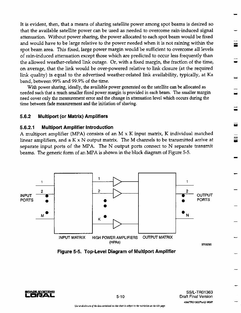
It is evident, then, that a means of sharing satellite power among spot beams is desired so
that the available satellite power can be used as needed to overcome rain-induced signal
attenuation. Without power sharing, the power allocated to each spot beam would be fixed
and would have to be large relative to the power needed when it is not raining within the
spot beam area. This fixed, large power margin would be sufficient to overcome all levels
of rain-induced attenuation except those which are predicted to occur less frequently than
the allowed weather-related link outage. Or, with a fixed margin, the fraction of the time,
on average, that the link would be over-powered relative to link closure (at the required
link quality) is equal to the advertised weather-related link availability, typically, at Ka
band, between 99% and 99.9% of the time.
With power sharing, ideally, the available power generated on the satellite can be allocated as
needed such that a much smaller f'Lxed power margin is provided in each beam. The smaller margin
need cover only the measurement error and the change in attenuation level which occurs during the
time between fade measurement and the initiation of sharing.
5.6.2 Multiport (or Matrix) Amplifiers
5.6.2.1 Multiport Amplifier Introduction
A multiport amplifier (MPA) consists of an M x K input matrix, K individual matched
linear amplifiers, and a K x N output matrix. The M channels to be transmitted arrive at
separate input ports of the MPA. The N output ports connect to N separate transmit
beams. The generic form of an MPA is shown in the block diagram of Figure 5-5.
a
EB
l
m
m
U
I
m
i
INPUT •PORTS •
M
INPUT MATRIX
' E>2 i>
HIGH POWER AMPLIFIER,c(HPAs)
OUTPUT MATRIX
Figure 5-5. Top-Level Diagram of Multiport Amplifier
2• OUTPUT• PORTS
N
9708293
N 13Y!B'I"l_M6
I.I=II_/_L 5-10
Use or disclosure o/the data contained on this sheet is sub_t to the restr_tion an the title page.
SS/L-TR01363Draft Final Version
45M/l'RO1363/Part2/-_
w
_r
=--
w
Signals in one channel arrive at one of the M input ports and are passed through a K-way,
uniform amplitude power divider. Each of the K outputs of the divider are sent, via phase
shifters, to the input of a separate one of the K amplifiers where it is summed with the
power-divided outputs from each of the other M-1 input channels. The composite signal,
all M signal units, is amplified by the corresponding amplifier. Thus, all M input signals
are proportionally represented in and amplified by all K individual amplifiers. It is seen
that sharing of amplifier power is easily achieved merely by setting the relative drive levels
of the various signals into the multiport amplifier while maintaining linear operation of all
amplifiers.
The M distinct signal units at each of the K amplifier outputs, one from each of the M input
ports, are, in turn, passed through K N-way uniform power dividers. Each output of an N-
way divider is then routed, via a phase shifter, to one of the output ports where it is
summed with the power-divided outputs from the other K-1 amplifiers. As a result, the
signal arriving at each output port consists of MK different signals, K of which originated
from input port 1, K from port 2, and so on through the K which originated from port M.
The K units which originated from port I have traversed different paths through both the
input and output matrices and, therefore, may each be imparted a phase shift such that
their vector sum is unity or zero. In certain implementations, this sum can be other rational
numbers. In any event, the sum determines whether or not a routing connection exists
between input port m and output port n. Thus, the multiport amplifier can route the
signals from one of M input ports to one or more of the N output ports.
The attraction of the MPA lies in its ability to share the power of several matched
amplifiers among several signals and, secondarily, to route inputs to more than a single
output. If the drive level into the MPA of any one of the signals is reduced, the output level
of that signal from the MPA will be correspondingly reduced. If the operation of the
amplifiers is maintained at a fixed backoff from saturation to achieve linearity, the power
may be shared among all the signals being amplified, from whatever input channel, merely
by adjusting their relative input levels. In this regard, it is our opinion that a TWTA and
linearizer, i.e., an LTWTA, optimized at, say 4 dB to 4.5 dB OBO (to achieve close to 20 dB
noise power ratio (NPR)) could achieve approximately 35% to 40% efficiency.
The discussion presented here draws liberally from a 1993 report [37] by X.T. Vuong, H.
Paul, and D. Cole of SAIC entitled Matrix Amplifier and Routing System (MARS) which was
prepared for the USAF Space and Missile Systems Center (SMC). The supporting study
investigated the use of matrix or multiport amplifiers in future X-band (7-8 GHz) military
satellite communications payloads.
5-11
Use or disclosure of the data contained an this sheet is subject to the restriction on the title page.
SS/L-TRO 1363Draft Final Version
4$M/rRO 1363/Pa_./- 9597

5.6.2.2 Non-Ideal Considerations
The following considerations may reduce the near-ideal sharing capability just described.
First, what makes the multiport amplifier attractive in the first place may also be a limiting
factor. Since each of the K individual amplifiers simultaneously amplifies all signals to be
transmitted by all of the N transmit beams it must be broadband. The required width of
the individual amplifier bandwidth depends on the frequency plan of the system. Usually,
this will not pose any limitation as bandwidths of I GHz are common for 20-GHz TWTs.
The K individual amplifiers must also operate in linear mode. In this mode an amplifier is
usually less efficient than in saturated mode. Onemight think of using a dual-mode TWTA
optimized for high efficiency in both a reduced-power mode and at nominal saturation, as
discussed in section 5.6.5. As noted there, however, the linearity of a dual-mode TWTA
optimized for high efficiency is very nearly the same as for a single-mode TWTA at
saturation. Therefore, a dual- or multi-mode TWTA cannot be used in an MPA.i
Finally, the output matrix is not lossless. In addition to the insertion losses of the
components of the matrix, there are combining losses. These comgining losses can be
significant if the matrix is realized using microwave combiners and separate phase shifters.
However, the combining losses are eliminated if the matrix is realized using a Butler or
hybrid matrix where signals are combined using hybrids.
Also, the multiport amplifier does not require an output multiplexer. Since the amplifiers
operate in their linear region, all multiplexing can be accomplished at low power level
prior to the input matrix. That is, each of the M signals arriving at the M input ports of the
multiport amplifier may originate from a corresponding single receive antenna beam or
may be a multiplex of signals that individually arrived on many different receive beams. It
is also possible that the multiport amplifier provide routing of signals from a single input
port to more than one output port and at more than one relative power level.
5.6.2.3 Implementation Issues
The two major questions in regard to a multiport amplifier are, first, is the implementation
practical at Ka band and second, how many individual amplifiers can be shared in a single
multiport amplifier?
Four facets of the implementation issue are discussed by Vuong, Paul, and Cole:
1. Insertion loss of the output matrix
2. Effect of errors in amplitude and phase settings resulting from the input matrix,
output matrix, and HPAs
3. Effects of HPA failure
4. Effects of HPA non-linearity
= =
I
w
N
U
Hg
I
I-DI'_aE_i,. 5-12
Use or disclostare of the data contained on this sheet is subject to the restriction on the title page.
SS/L-TR01363Draft Final Version
45 MrrR01363/P ar t2J-9F--_T/

. =
=
Summary discussions of these issues are given below.
Regarding the number of amplifiers, K, that can be shared, according to Vuong, Paul, and
Cole: "to have the desired orthogonality among the output ports, the number of output
ports N must not exceed the number of amplifiers K:" That is, K > N. Other than this
restriction, there does not seem to be a limit to K other than that of the obvious physical
limitation of fitting K amplifiers into the spacecraft and providing the requisite input and
output matrices.
As for the number of amplifiers required to serve a given number of beams, the required
number K will depend upon N, the total number of beams served by the multiport
amplifier; upon Y, the total number of carriers served by the MPA; upon X, the number of
carriers that simultaneously experience high fades; upon PL, the linear power contributed
by each of the K amplifiers; and upon Ps, the power required from the MPA per downlink
carrier in clear weather. To get a sense for the value of K, it was calculated for several
values of N and X using four values of PL and a Ps of 6.2 W (see link budget shown in Table
5-1). Further, these calculations assume a single carrier per beam (i.e., Y=N).
Table 5-2 gives the resulting values of K based on the equation
KP L = (62"X + 6.2*(N-X)) or K = (62"x + 6.2*(N-X))/PL,
where KP L is the available linear RF power and 62"X + 6.2*(N-X) is the required linear RF
power. Note that the power provided to each of the X carriers that experience high fades is
increased by 10 dB over the clear-weather value of 6.2 W. In actual practice, the total excess
power given to these X carriers could be distributed among them in any proportion, it need
not be uniformly distributed.
Supposing a saturated HPA power of 120 W, the PL values used here of 25 W, 31.6 W, 39.8
W, and 50 W correspond to HPA output back0_ffs of 6.8 dB, 5.8 dB, 4.8 dB, and 3.8 dB,
respectively.
From Table 5-2, it is apparent that an MPA provides significant capability to counter
downlink rain fades. Even for the smaller P_. values, link closure in all beams occurs when
fully one third of the beams are experiencing high downlink fading. Contrast this with the
probability that rain occurs in any given beam no more than about 5% of the time for most
areas of the world. For the higher values of PL, service is maintained when up to
approximately 80% of the downlink beams experience high rain fades.
a--Dr_a_L 5-13
Use or disclosure of the data contained on this sheet is subject to the restriction on the title page.
SS/L-TR01363Draft Final Version
45 M/FR 01363/Pa rt2J- 9Fo,_7

Table 5-1. Link Budget for Ka-band Demod-Decode/Recode-Remod Payload
Transmiffing 60 Mb/s per 0.6-deg Beam into 70 cm receive terminalm
Ka-band budqet assuming a rate 3/5, K=7 convolutional code concatenated with a rate 0.9216 R-S block code.On-board decoding. RequiredLink burst (dat_ bits) rateUser terminal elev. anqleSatellite altitude
Earth radius
Slant rangeJ
Total xm|tt__l_owe dbeam
Tx antenna diameter
Eb/No values are taken from CyberStar filing with0,384120,001
35786.00!
6378.0039554.46
Uolink1.000.00
29.5044.50
0.70
0.70TX antenna beamwidth 1.02
Antenna efficiency 60.00Transmission fr.e.quencyAqtennae_ainPointin._,EOC & lin_ IOS,S l
EIRP per userI 43.80Free space loss 213.79Atmos, loss 1.00R._ainloss 0.00
I Path Loss 21 4.79Rx antenna diameter 0.65Rx antenna beamwidth 1.1 0
Antenna efficiency 55.00Antenna peak gain 43.42Pointing loss & polar, mis,. 3.23
Gain at antenna flange .... 40.19 I290.00N/A
1.00
Rx clear-=sky ant. noise tem__.Rx rainy-sky ant. noise temp.__Line loss I
LNA+ noise figure i 2,16TSySTr (in rain_ at flan.o.e) 600.34
'1 I _ G/T 12.41Received siqnal (flange,. rain)!_ .-_130.80kT, in rain (if any)C/No I
-200.8270.0115.0070.8467.40
200.00
the FCC (9/29/95)._ .....60.00|Midis I FECcoderatp= 0.55 I R-S code rate=; 0.9220.00,[de:1 I _3onv. code rate= 0.60
3578..6.001kr_ I Modulation= _I Hz/=svm/sec=: 1.5(t I
6378.00 km I == Uplink signal bandwidth (MHz)= I 0.5;
39554.46Ikm I Downlink si_lnal bandwidth (MHz)=I 81.3_Downlinkl Total RF pow_erradiated (assumed), W= 400
4.041W Tot RF pwr/bm13.14 I # active beamsl1286.06idBW ..... Total downlink mar.qip / beam, dB 0.00
1.781m Array dia.=21/if(GHz)*BW(deg)); with taper0. 600', dl_j E /55.00!% Direct radiating elements with taper
GHzdBidBdBWidBdB
19.7048.69
4.1050.65
210.281.000.00 dB
211T28 dB0.70]m1 52]_j
55.001%40,60]dBi
I 0.53 dB40.07 dB75.48!K
75.48 K1.00 dB1.50 dB
301.18!K15.28 dB/K
-120.57-203.81
Link interference (C/I) -Link interference_C/Io___C/(No+Io) IRain-induced c ross_0_o_lC/(No+Io+Xo)ILink data rate (dB-Hz)
Recl'd Eb/No lw/impI, loss 1A._vailable m.ar.qin
I
83.2415.0092.7882.79
200.0082.7967.40
55.84 77.78
dBWdBW
dB-Hz
8.00
3.561
NASA Hdbk p. 6-7_foi elev. angle x 1.22
dB-Hz_dBdB-Hz
5.OOIdeO.O01dB
i i
i User rx bw (°)
I1.52
_lear Skv: ITa=17.89+280*(1-10^(-Latmos/10)Rainy Sky: I
ITa= 1"7.89+280" (1-10^(- (Latmos+Lrain)))
JI
Including C/IM from active antenna amplifiersC/Io = C/I+10*LOG10(Rb) in data bandwidth
LCircular polarization. In data rate bandwidth.
1
i
1
1
1
i
N_
LD_I. 5-14
Use or disclosure of the data contained on this shee_ is subj¢_ 1o lk¢ restriction on the title page.
SS/L-TRO 1363
Draft Final Version
45 M/TR01363JPa rt2J- 9F_971
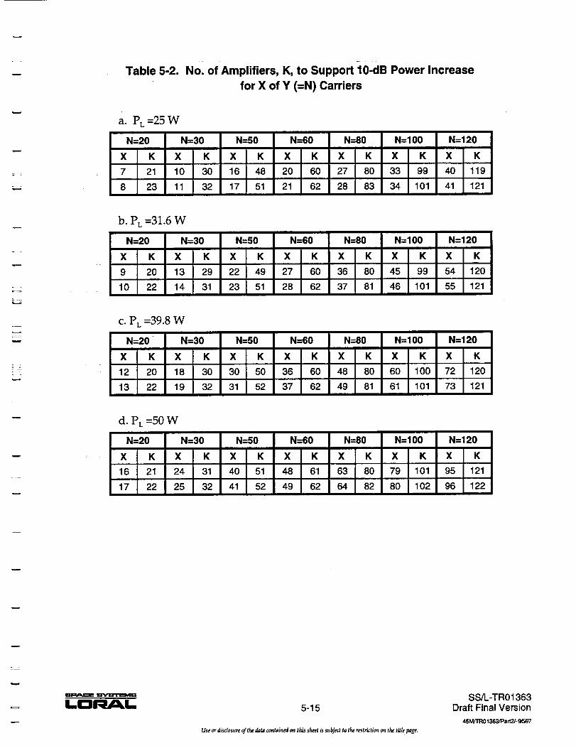
w Table 5-2. No. of Amplifiers, K, to Support 10-dB Power Increase
for X of Y (=N) Carriers
a. PL =25 W
N=20 N=30 N=50
X K X K X K
7 21 10 30 16 48
8 23 11 32 17 51
N=60
X K
20 60
21 62
N=80
X K
27 80
28 83
N=100
X K
33 99
34 101
N=120
X K
40 119
41 121
w
_r..a
2 _:
b. PL =31.6 W
N=20
X K
9 2O
10 22
N=30
X K
13 29
14 31
c. PL =39.8 W
N=20 " N=30
X K X K
12 20 18 30
13 22 19 32
N=50 N=60 N=80
X K X K X K
22 49 27 60 36 80
23 51 28 62 37 81
N=50 N=60 N=80
X K X K X K
30 50 36 60 48 80
31 52 37 62 49 81
N=100 N=120
X K X K
45 99 54 120
46 101 55 121
N=100 N=120
X K X K
60 100 72 120
61 101 73 121
d. Pt =50 W
N=20
X K
16 21
17 22
N=30
X K
24 31
25 32
N=50 N=60 N=80 N=100
X K X K X K X K
40 51 48 61 63 80 79 101
41 52 49 62 64 82 80 102
N=120
X K
95 121
96 122
w
LDI'_/_I,,, 5-15
Use or disclosure of the data contained _a this sheet is subject to the restriction on the title page.
SS/L-TR01363Draft Final Version
45 M/TR01363/Part2/- 9_J7

Obviously, during any system implementation the linear power per amplifier would be
matched to the expected broad area rain statistics such that total power per MPA is
minimized.
5.6.2.3 Insertion Loss of the Output Matrix
The multiport amplifier output matrix consists of k stages of hybrids, where the number of
amplifiers, K, is given by K=2 k. It is assumed that this output matrix would be realized in
waveguide rather than, for example, squareax or a printed network. The output loss figure
given here does not include the waveguide for connecting the N output ports with the N
antenna beam input ports nor does it include the output zonal filters. A value of 0.4 dB to
0.5 dB per stage is estimated at 19 GHz when realized as a hybrid ring. (This compares to a
0.5-dB loss per stage estimate at X-band (7.5 GHz) given by Vuong, Paul, and Cole.)
For an MPA with 128 amplifiers, there would be 7 stages of ring hybrids, or an output
matrix loss of approximately 3.0 dB. This is to be compared to an output loss, not
including filter, of about 0.5 dB for either the active transmit lens array or the active
transmit phased array antennas. However, as will be mentioned below, these two active
antennas depend upon the use of SSPAs rather than TWTAs and would, therefore, have
lower efficiency amplifiers.
5.6.2.4 Phase and Amplitude Deviations
A concern associated with MPAs is the ability to achieve nearly identical insertion phase,
aside from intended phase shifts, and amplitude through the multiple paths of the input
and output matrices as well as the ability to phase and amplitude match the K amplifiers
themselves. Certainly, without very close phase and amplitude matching of these paths,
the vector sums of the component signals at the MPA output ports will neither sum to zero
at unwanted ports nor sum to unity at wanted ports. A non-zero sum at unwanted ports,
i.e., in unwanted beams, reduces port-to-port isolation, I_o. In other words, it creates
interference in frequency reuse schemes. Frequency reuse is one of the primary means of
achieving high capacity in all of the Ka-band multimedia filings. A non-unity sum in
wanted beams means a defacto loss, AC, as if an ohmic loss had been inserted after the
amplifiers. In the ideal, no degradation, case, AC = 0 dB and I,o = oo dB.
The tolerance on amplitude and phase tracking among the several signal paths was
investigated by Vuong, Paul, and Cole in both a worst-case analysis and a Monte Carlo
analysis. The worst case analysis is the easier analysis. The Monte Carlo analysis was
undertaken in order to "consider the nominal system performance based upon statistically
random phase and amplitude deviations that reflect the use of typical components." Also,
while "worst case results may provide information that is safe to create specifications for
the design of [an MPA] and its components, these specifications may be too tight to meet in
a cost-effective manner."
I
U
m
m
mm
m
m
m
N_
LD_L 5-16
Use or disclosure of the data contained on this sheet is subject to the restriction on the title page.
SS/L-TR01363Draft Final Version
45 M/TR01363/Pa rt2J'-9FJ97

w
The results of these analyses are shown in Figures 5-6 through 5-10. The worst-case
analyses are summarized in Figures 5-6 and 5-7. The Monte Carlo analysis is summarized
in Figures 5-8 through 5-10. In these figures, AG = 20 log(1/(1 - a)), where a = maximum
allowable amplitude deviation in relative voltage ratio and Ao = maximum allowable phase
deviation (degrees). Note that in voltage ratio, the maximum overdeviation allowable is
the same as the maximum underdeviation allowable, which is c_ (A is the nominal carrier
amplitude). When converted to dB, they are no longer the same due to the nonlinear
nature of the logarithmic function; the maximum overdeviation allowable becomes AG ÷ =
20 log(1 + c_) dB, and the maximum underdeviation allowable becomes AG" = 20 log(1/(1 -
_)) dB. The values of AG ÷ and aG are approximately the same when r_ is small with
respect to unity.
: z
5O
(9w0 40
Z0
w
-1- 20cOU.lo9
"1-o.
<
WORST CARRIER POWER DEGRADATION (dB)
INPUT MATRIX/HPN OUTPUT MATRIX
3 dB
2
1
0.5
0 0.5 1 1.5 2 2.5 3 3.5
MAX. GAIN DEVIATION _G (dB) 97o8294
Figure 5-6. Contours of Worst-Case Carrier Power Degradation _C Versus
Maximum Allowable Phase Deviation be and Gain Deviation _G of Input
Matrix, HPAs or Output Matrix
i
m_
La_L 5-17
Use or disclosure of the data contained on this sheet is subject to the restriction on the title page.
SS/L-TR01363Draft Final Version
45M/TR01363/Part2/-_Ir-_97

12
WORST PORT - PORT ISOLATION (dB)
OLU
Ctv
zO
>LUOLU
09
,<
-1-12.
6 o
15 dB
2O
25
3O
\\
\\
\\
\\
\
-- -- - INPUT MATRIX / HPAOUTPUT MATRIX
\\
\\
\\
\\
t
0 0.2 0.4 0.6 0.8 1.0 1.2 1.4 1.6 1.8
MAX. GAIN DEVIATION AG (dB) 97o_9s
Figure 5-7. Contours of Worst-Case Port-Port Isolation Iso Versus
Maximum Allowable Phase Deviation be and Gain Deviation AG of
Input Matrix, HPAs or Output Matrix
Vuong, Paul, and Cole generated worst-case port-to-port isolation results for K=4, 8, and 16
and found them to be identical. They state, therefore, that "It is reasonable to extrapolate
that the same worst case results are also expected for any K= power of 2. No attempts have
been made, however, to prove mathematically that the worst case port-port isolation
results are indeed indentical for any K= power of 2."
5.6.2.5 Providing Redundant HPAs
If no redundancy were provided, HPA failures would reduce the power available at the
"wanted" port_.and decreas e the isolationof the"unwanted" ports. The power at the
wanted port is the sum of K vectors, all aligned in phase. Therefore, the reduction in power
from failure of L out of K HPAs is given by:
AC = 20 logl0(K/(K-L)) dB
!
l
BB
m
I
I
IBII
m
m
b
L
m
w
m
u
LI=II'_M_L 5-18
Use or disclosure of the data contained on this sheet is s=,.b_ect to the restriction on the title page.
SS/L-TR01363Draft Final Version
45M/TFt01363/Part2/-gFJ97

w
L_ 90LU
a 80
z 700
6o
>w 50D
,17-4o"l-co 30UJ
< 20I0-
10
_ 0
CARRIER POWER DEGRADATION (dB)MONTE CARLO SIMULATION RESULTS
2 dB
- 1
- N
-L \_ \0.2 \
t II, I I! I
t I
0 1 2
AVERAGE
-- -- - AVERAGE + 2*SIMGA
2 dB
N
\\ 0.5
\
| _ 0.2I I
,.l , i , t , i , i i i I i , i , i _3 4 5 6 7 8 9 10 11 12
MAX. GAIN DEVIATION AG (dB) 9708296
m
L
u
m
w
m
Figure 5-8. Contours of Average and (Average +2 x Sigma) of Carrier Power
Degradation AC Due to Random Deviations in Characteristics of Input Matrix, HPAs
or Output Matrix (K ---8 and # Monte Carlo Cycles = 20,000)
The isolation at unwanted ports depends upon pairwise cancellation of the K vectors. In
the best case, the L failed HPAs would be paired such that the remaining K-L vectors
would still cancel except when L is odd, in which case a single vector would remainuncancelled. In the worst case, L vectors would remain uncancelled and be aligned. The
associated isolations, which establish the upper and lower bounds, are:
I_o (best case) = 20 logl0(K-L) dB where L is odd
= oo dB where L is even
I_o (worst case) = 20 Iogl0((K-L)/L) dB
A table of values of AC and I,o taken from Vuong, Paul, and Cole showing their
dependence upon K and L is given in Table 5-3. Note that for large K and for ideal input
and output matrices (i.e., phases set according to ideal MPA theory), both the worst-case
reduction in power and the worst-case isolation are probably acceptable. Nevertheless, it
would be prudent to provide redundant amplifiers. Care must used in how the associated
switching is accomplished so that the desired phase relations among output vectors are not
perturbed when redundant units are brought into use.
EDgE 5-19
Use or disclosure of the data containtd an this sheet is subject to the restriction on the title page.
SS/L-TR01 363Draft Final Version
45M/TR01363/Part2/-gr'o/97

15
ISOLATION VS INPUT MATRIX/HPA CHARACTERISTIC DEVIATIONSMONTE CARLO SIMULATION RESULTS
AVERAGE
-- -- - AVERAGE - 2*SIGMA
(.9LUE3v
ZO
>UJt7
111
<I
< \25
25
\
\\20 dB
2O dB
30
\30
t
\35 I
35 II
0 0.5 1 1.5 2 2.5 3 3.5
MAX. GAIN DEVIATION _G (dB) 9_0829_
Figure 5-9. Contours of Average and (Average +2 x Sigma) of Port-Port Isolation Iso
Due to Random Deviations in Characteristics of Input Matrix or HPAs
(K = 8 and # Monte Carlo Cycles = 20,000)
i
m
I
!
m
i
BIB
g
i_
LDI' M L 5-20
Use or disclosure ofthe da_a contained on this sheet is s_bject to the rest_'_c_ionon the titlepage.
SS/L-TR01363Draft Final Version
45M/TR01363/PartPJ-9FJ97
m
I

2 .
w
m
w
ISOLATION VS OUTPUT MATRIX/HPA CHARACTERISTIC DEVIATIONSMONTE CARLO SIMULATION RESULTS
15
12-
L9LUE3v
z_o
>uJE3
I09LU09<"1-
30\
35
35 I
00
Figure 5-I0.
I
0.5
-- AVERAGE
-- -- - AVERAGE - 2*SIGMA20
\ \20
\
25 I
III
IIIIII
2.5 3
I ! I I I
3.51 1.5 2
MAX. GAIN DEVIATION AG (dB) 9708298
Contours of Average and (Average +2 x Sigma) of Port-Port Isolation
Iso Due to Random Deviations in Characteristics of Output Matrix or HPAs
(K = 8 and # Monte Carlo Cycles = 20,000)
5-21
Useordisclosureof the data contained onthis sheetis subjecfto the restriction onthe title page.
SS/L-TR01363Draft Final Version
45 M/TRO 1363/Part2/- _r-_7
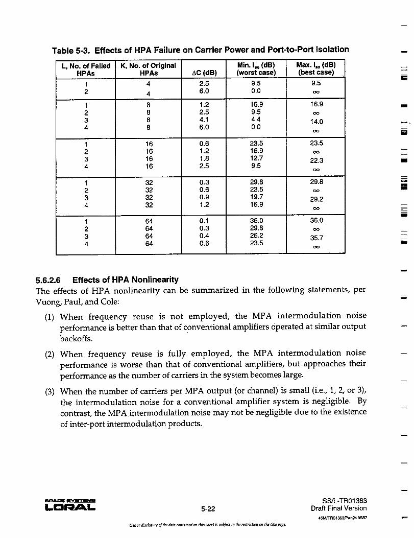
Table 5-3. Effects of HPA Failure on Carrier Power and Port-to-Port Isolation
L, No. of FailedHPAs
12
1234
1234
1234
K, No. of OriginalHPAs
4
4
8888
16161616
32323232
64646464
AC (dB)
2.56.0
1.22.54.16.0
0.61.21.82.5
0.30.60.91.2
Min. I,o (dB)(worst case)
9.50.0
16.99.54.40.0
23.516.912.79.5
29.823.519.716.9
0.10.30.40.6
36.029.826.223.5
Max. I,o (dB)(best case)
9.5Oo
16.9OO
14.0
OO
23.5oo
22.3
oo
29.8co
29.2
36.0OO
35.7
OO
i
BIB
BI
BB
iII
lib
m
BII
5.6.2.6 Effects of HPA Nonlinearity
The effects of HPA nonlinearity can be summarized in the following statements, per
Vuong, Paul, and Cole:
(1) When frequency reuse is not employed, the MPA intermodulation noise
performance is better than that of conventional amplifiers operated at similar output
backoffs.
(2) When frequency reuse is fully employed, the MPA intermodulation noise
performance is worse than that of conventional amplifiers, but approaches their
performance as the number of carriers in the system becomes large.
(3) When the number of carriers per MPA output (or channel) is small (i.e., 1, 2, or 3),
the intermodulation noise for a conventional amplifier system is negligible. By
contrast, the MPA intermodulation noise may not be negligible due to the existence
of inter-port intermodulation products.
u
m_
5-22
Use or disclosure of the data contained an this sheet is subject to the restriction an the title page.
SS/L-TR01363Draft Final Version
45 M/TR01363/Pa rt2/- 9FJ,97

u
w
m
i
w
5.6.3 Active Transmit Lens Array
An active transmit lens array (ATLA) antenna has four major sections, three of which
comprise the RF lens. The fourth is a feed array. These sections, shown in an artists sketch
of a proof of concept antenna in Figure 5-11, are:
(1) A fiat array of radiating elements launches the far-field spot beams.
(2) A corresponding array of power modules, one for each radiating element, supplies
signal power to the radiating array. Each power module contains an amplifier and a
delay line. Collectively, the delay lines of the modules constitute the center portion
of the lens.
(3)
(4)
Signals arrive at the modules from individual receive elements at their inputs.
The receive elements are space fed, in turn, from an array of feed horns that is
physically separate from the lens. Each far-field beam is created by the signals
transmitted from a single feed horn. The beam direction is fixed by the location of
the feed horn in the feed array.
"1
©O _'_ FEEDARRAY
=--=
m
.. FAR-FIELD POWER RECEIVERADIATING ARRAY MODULES ELEMENT ARRAY
97O8299
Figure 5-11. Active Transmit Lens Array Antenna Concept
u
u
LC:II'_/_L 5-23
Use or disclosure of the data contained on this sheet is subject to the restriction on the title page.
SS/L-TRO 1363Draft Final Version
45M//1:_01363/Pa_2/- 9r-_97

The attraction of the ATLA is that no beam forming networks, per se, are required. Thus,
in principle, a major difficulty encountered in the ATPA concept is avoided. The beam
forming network is the lens which forms all beams simultaneously with directions
determined by the geometry of the feed array and lens structure.
Both the ATLA and the ATPA lend themselves to solid state power amplifiers (SSPAs);
thus heat dissipation remains a common challenge. For large arrays, creating several tens
of beams each transmitting carrier data rates in the 60 to 100 Mb/s range, the power
dissipation problem is acute.
These two similarities of the ATLA and the ATPA mean that their weights are comparable.
As such, the above ATPA weight estimate, to a first order, applies to the ATLA also. A
closer look at weight would likely show that the ATLA weighs slightly less than the ATPA
because it does not have the multiple beam forming networks.
As with the ATPA, a major impediment to the ATLA technology is cost of the lens itself
and, specifically, of the several hundred power modules. At Ka band, as noted above, a
large number of modules is indicated for two reasons. First, the small size of the
corresponding radiating elements means that a large number of such is required to create
the desired narrow beamwidths. Second, the relatively small power available in Ka-band
SSPAs means that tens of high-power beams require a large number of modules to achieve
the total power.
5.6.4 Active Transmit Phased Array
Based on work done for Globalstar and on engineering work for an active transmit phased
array (ATPA) antenna at Ka band (20 GHz) [38], it is known that the use of ATPAs for
more than a relatively few beams from the same aperture is not practical. The difficulty
arises in creating the beam forming networks (BFNs), one for each beam, in a physically
small space. Each BFN must have the same number of outputs as there are antenna
elements. Furthermore, an output from each BFN must be summed with corresponding
outputs from all other BFNs to feed each one of the antenna elements. As the number of
beams and antenna elements grows, the physical task becomes overwhelming just from a
topological viewpoint. Globalstar achieves 16 beams. It is believed that Iridium also
achieves 16-beams (from the FCC filing for Iridium, 48 beams per satellite are created in
three separate phased arrays). The FCC filing for M-Star states that up to 32 beams are
created in a single phased array. Although not a clear confirmation of the limited beam
capacity, these are certainly indicative. In terms of the numbers of beams which are
indicated in the current Ka-band multimedia filings, shown in Table 5-4, 16 beams is small.
Even 32 beams (note that this antenna is only conceptual at this juncture; it has not been
built) is fewer than is shown for all but one of the systems.
m
u
IBm
t
BB
m
ii
mp/M¢_! I'V'I_TEM_
LC:I_I-- 5-24
Use or disclosure of t_ data contained on this sheet is subject to the restriction on the title page.
SS/L-TR01363Draft Final version
45M/'i'R01363/Pa rt2/- _,97
m
m

i
m
Table 5-4. Representative Ka-band Systems with Number of Beams per Satellite
System Astrolink CyberStar NetSat 28 Spaceway Teledesic Voice Span
Company L-M SS/I_ NetSat 28 HAC Teledesic AT&T
No. Beams 192 27 1000 48 64 64
5.6.5 Comparison of Total DC Power
The results of a first-cut analysis of total required DC power for the three sharing
approaches (ATLA antenna, ATPA antenna, and MPA) for 128 beams and a required 60
Mb/s per beam into a 70-cm ground receive terminal are shown in Table 5-5. For each
sharing approach, the per-carrier EIRP of 50.65 dBW is taken from Table 5-1. The number
of active elements (i.e., SSPA transmit modules) for the active phased array and the active
lens array are shown in Table 5-6. For the multiport amplifier, there is an active amplifier,
which is assumed to be a TWTA, for each of the 128 beams.
Table 5-5. Total DC Power for Three Transmit Power-Sharing Approaches
(assumes required EIRP of 50.65 dBW, 128 0.6-deg spot beams with
48.7 dBi peak gain)
__=
r
_=_
Parameter ATLA ATPA MPA
Loss to EOC 3.0 dB 3.0 dB 3.0 dB
Output loss (w/filter) 1.1 dB 1.1 dB 3.7 dB
Antenna peak gain 48.7 clBi 48.7 dBi 48.7 dBi
Req'd RF pwr per beam at HPA output 6.05 dBW 6.05 dBW 8.65 dBW
(4.03 W) (4.03 W) (7.33 W)
Total Req'd RF pwr (=128 x above line) 515.8 W 515.8 W 938.2 W
HPA linear mode efficiency 14% 14% 45%
Total DC Power 3685 W 3685 W 2085 W
m
w
m
Table 5-6. Number of Active Transmit Modules (or Elements) for
Three Sharing Technic ue
Parameter ATLA ATPA MPA
Rated RF power per transmit module, 1.0 W 1.0 W 25 Wassumed
HPA OBO, assumed 4.09 dB 4.09 dB 5.33 dB
RF power per transmit module 0.39 W 0.39 W 7.33 W
Number of active transmit modules 1323 1323 128(=515.8/0.39) (=515.8/0.39) (=no. of beams)
Diameter of array, approximate at 43 antenna 43 antenna19.2 GHz (see Appendix B) elements elements N/A
69 inches 69 inches(at 2.6_, spacing) (at 2.6_, spacing)
LC:IIRbC_L- 5-25
Use or disclosure of the data contained on this sheet is subject to the reslriction on the title page.
SS/L-TR01363Draft Final Version
45M/'rR01363/Patt2/-9_,97'

The power dissipated and the size of the corresponding radiator for each sharing technique
is indicated in Table 5-7 based on plausible efficiencies for the SSPA and TWTA units. This
power is the sum of the power dissipated in the output loss and the power dissipated by
the transmit modules themselves. The radiator size shown assumes a radiator capacity of
60 W/ft 2. A value of 45 to 50 W/W would be reflective of current capability.
What can be concluded from the above comparison? First, the power required for a large
array-type sharing technique is about twice that required for an MPA technique. That is, of
the two primary contributors to DC power differences, i.e., HPA efficiency and output
circuit losses, the lower efficiency of the SSPAs dominates. Therefore, even with nearly a
4-dB output circuit loss, the MPA power, for the same EIRP per beam, is half that of the
array techniques. Second, the additional power dissipation of the array-type techniques
also requires larger solar arrays to generate the increased power and larger radiators to
reject the heat.
An estimate of the increased weight associated with the larger power subsystem and the
larger radiators, not to mention the increased difficulty of integrating the radiators into the
spacecraft configuration, may be obtained. A current nominal value for Watts per pound
for solar-power subsystems on large geosynchronous satellites with 12 year lifetimes is
about 10 W per pound of total power subsystem weight. In the above comparison, the
array-type techniques must generate 1600 W more DC power than the MPA technique.
This would, nominally, translate into a power subsystem weighing 160 lbs more.
For the radiator panels (heat pipes embedded in aluminum honeycomb with face skins and
optical solar reflectors (OSRs)), a nominal weight is 5 gm/in 2, or 1.6 lb/_. Therefore, the
weight difference occasioned by the larger radiators is approximately 44 lbs (=1.6 x 4.6 x 6).
The total weight difference arising from these considerations is approximately 200 lbs. A
BIB
L--
ml
=__I
I
im
[]
lib
BI]
Table 5-7. Power Dissipated and Radiator Size for the Three Sharing Techniques
Parameter ATLA ATPA MPA.r
Total DC power (per Table 5.6-2) 3685 W 3685 W 2085 W
Power dissipated at transmit module
Power dissipated in output loss
3169 W
116W(=516 x (1-10"° 11))
3169 W
116W(=516 x (1-10-°"))
55 sq. ft.(=3285/60)
1147W
538 W(=938 x (1-10°3'))
55 sq. ft.(=3285/60)
Total RF power dissipated 3285 W 3285 W 1685 W
Required radiator area
Dimensions of two radiator panels
28 sq. ft.(=1685/60)
4.6 x6 ft. 4.6 x 6 ft. 4.6 x3 ft.(two) (two) (two)
w
m_
5-26
Use or disclosure of the data containt, d on this sheet is subject to the restriction on the tit_ page.
SS/L-TR01363Draft Final Version
45M/TRO1363/Part2/-95B7 m

w
w
w
r__
complete comparison of mass should include the array antennas themselves versus the
multiple beam reflector antenna postulated for use with the MPA. It is believed that this
comparison favors the reflector antenna.
Another consideration is the cost of the systems. Active arrays are much more expensive
than are reflector antennas. The cost difference would be magnified for arrays with 50 to
100 beams compared to a reflector multiple beam configuration. It would be magnified
even further to make good on the promise of arrays of beam steering and shaping. The
cost of the input and output matrices for the MPA would not narrow the difference
appreciably.
5.6.6 Multimode Amplifiers
A multimode amplifier is designed so as to achieve near maximum efficiency when
operated at saturation as well as when operated at selected output power levels below this
saturation level. Thus, if it is not raining in the area of a given spot beam, the amplifier for
that beam could be run at reduced output power while still operating near peak efficiency.
The DC power required to run the amplifier would be reduced in the same proportion
(assuming no loss in overall efficiency)as is the output power and would be available for
application to an amplifier connected to a beam whose area is experiencing rain. In this
manner, the total DC power allocated to the satellite I-tPAs can be shared and could be
much less than without this sharing, as discussed above.
This technology would be ideal for reflector multiple beam antennas (MBAs) where each
beam is fed, typically, by a single HPA. It allows redundant amplifiers to be provided in
the usual fashion, does not require large beam forming or switching networks to
accomplish power sharing, is straight-forward and relatively simple to implement.
However, while the multimode feature drops the output power level with very little loss in
efficiency, it also drops the gain and has very little effect on the linearity. In other words, a
multimode TWTA cannot be used for linearity enhancement. Therefore, the multimode
amplifier would be used only in systems with a single carrier per HPA.
In almost all instances, the HPA of choice for this architecture would be a traveling wave
tube (TWT) amplifier (TWTA). Especially at Ka band, TWTAs are capable of much greater
power output and much higher efficiency than are solid state power amplifiers (SSPAs).
High capacity, one of the required system characteristics for the target system, translates
directly into high power HPAs. Thermal control considerations on the satellite also favor
the higher efficiency TWTAs.
One might suggest that reduced output power of the HPA be achieved by merely backing
off the drive level. However, because amplifier operating efficiencies fall drastically with
reduced drive levels, this approach is not practical. The necessity for multimode operation
m[--G_K,. 5-27
Use or disclosure of the data contained on this sheet is subject to the restriction on the title page.
SS/L-TR01363Draft Final Version
45M/rR01363/Part2/- 9FJ97

is seen by noting the approximate tube efficiencies for representative output power levels
of a single-mode tube shown in Table 5-8. These efficiencies assume a 20-GHz TWT
operated with a single carrier.
As a result of this loss of efficiency, even though the power consumption of a single-mode
TWTA decreases, the dissipated power stays relatively constant.
In addition to a TWT efficiency loss, two other effects accompany reduced output levels in
a single-mode TWTA and contribute to the attraction (at least in theory) of multimode
TWTAs. First, the gain of the TWT increases. Although not a problem, a calibration would
be required to determine the input backoff corresponding to a given desired reduction in
output power level. Second, the efficiency of the electronic power conditioner (EPC) for the
TWT would also drop. EPC efficiency varies with the processed power level. Typical EPC
efficiencies for saturated TWT loads are in the range of 92% to 94%. At large values of
OBO, where the total power consumption is reduced, the EPC efficiency will drop to as low
as 86% to 88%.
It should be noted, however, that other effects also must be considered when
contemplating use of a multimode TWTA. For output power reductions achieved by
adjusting the operating voltages (a multimode TWTA), the adjusted voltages cause a
decrease in cathode current in the TWT which, in turn, reduces the output power. The
reduction in effective current density through the tube reduces the gain per inch in the
TWT circuit. For any given physical geometry, the gain continues to drop as the current
density is reduced. For a 10 dB output power range, the gain of a single-mode TWT would
drop by at least 30 dB. [Below a certain threshold, usually around 30 dB, the TWT
efficiency will basically fall off a cliff because the tube requires a certain minimum gain
level in order to operate properly.] This change would have to be offset in the drive
circuits and would likely seriously perturb the phase of the signal being transmitted. It
would need to be determined whether the ground receiver could track through this
perturbation. Also, the statement made above regarding reduced efficiency of the EPC for
a single-mode TWT applies to a multimode TWT as well. When the processed power level
drops, whether in a single-mode or a multimode TWT, the EPC efficiency will drop.
Table 5-8. Representative Single-Mode TWT Efficiencies at Several
Output Backoff (OBO) Levels
TWT Operating Point Approximate TWT Efficiency
0 dB OBO (saturation)
3 dB OBO
10 dB OBO
20 dB OBO
58%
40%
15%
2%orless
m
IE;
m
W
.=..
BB
l
W
mm
I,.,¢:11_/_1.. 5-28
Use or disclosure of the data contained on this sh_ is subject _o the restriction an the title page,
SS/L-TR01363Draft Final Version
45M/'rR01363JPart2/- _97J

w
= :
w
L -
=
i
--=
!
To date, multimode TWTAs with the necessary span in output power have not been
realized. To offer significant rain fade mitigation at Ka band independent of other
approaches, a power level difference of at least 10 dB is desired. It is our opinion that a 10-
dB output power range using commandable voltage steps is completely impractical. While
dual and triple mode tubes for space have been achieved (none of which were built using
modem technology), the span in output power levels has not exceeded 6 dB. For example,
an L-band triple-mode TWTA was baselined for and flew on Marisat with nominal, 0 dB, 3
dB, and 6 dB OBO modes. Marisat was a very successful program.
Apparently, the number of power levels is not the efficiency driver. Rather, TWT efficiency
is a function of the span of the power range. Over an output power range of 3 dB, very
little loss of efficiency will occur. Over 6 dB, expect an efficiency drop of from 15% to 25%.
The resulting efficiency can be increased, theoretically, by increasing the complexity of the
EPC so that more than just the anode voltage is adjusted. This has, to our knowledge,
never been successfully implemented. One might envision separate EPCs in parallel, one
for each mode. However, EPCs and tubes must come on-line together and must be cycled
through a warm-up period prior to coming on line. The typical turn-on period is about 3
minutes. The consequent disruption to the transmitted signal would likely be
unacceptable. Also, this multiple EPC approach would be much heavier. These
considerations, to date, have meant that a multimode TWTA is almost never used because
the perceived benefits do not offset the added complexity and mass.
For example, in the ACTS program, a 1988 study [39] "compared the spacecraft resources
required for an operational system employing either dual-power TWTAs or fixed power
TWTAs using [then current] technology." The study found that "the ACTS dual-power
system ... offer[ed] no major advantages compared to a conventional ... fixed-power
system."
It should be stated that perturbations to the transmitted signal will be experienced not only
when changing the EPC, as mentioned earlier, but also when changing modes in a multi-
mode TWTA. For a very large power change (>6 dB), the carrier would likely have to be
taken down. It might also be necessary to turn off all high voltage in the EPC. At this
point, the warm-up cycle would be initiated and the overall downtime would be about 3
minutes.
In summary, the multimode TWTA for large (>6 dB) changes in output power appears to
be infeasible. For changes less than 6 dB, a multimode TWTA might be used in conjunction
with data and code rate changes to provide up to 16 dB of rain fade mitigation by halving
the data rate and simultaneously introducing rate one-half forward error correction coding.
Note, however, that development for such a multimode tube at Ka band was not successful
during the ACTS development and has not been reinitiated.
i.,D_L 5-29
Use or disclosure of the data contained on this sheet is su_ect to the restriction on the title page.
SS/L-TR01363Draft Final Version
45MtTR01363/Part2/-gF_97
5.6.7 Conclusions for Downlink Power Sharing
It is concluded that the multiport amplifier (MPA) offers significant promise for downlink
power sharing of many tens of downlink beams. In contrast, the active transmit lens array
(ATLA) and the active transmit phased array (ATPA) antennas would find application only
for relatively smaller numbers of total beams. This is not to say that the MPA will, after
considered engineering design effort, prove feasible at Ka band (20 GHz). Nevertheless, it
is believed to be feasible at this time. Vuong, Paul, and Cox concluded that an MPA was
feasible at X band (7.5 GHz). As discussed in section 5.5, power sharing by code and data
rate changes, is also feasible. The advantage of the MPA is there is no disruption to data
rate nor need for synchronization of code and data rate changes at the transmitter and at
the receiver.
m
m
I
Wm
i
i
gll_a_! S'WIIITImVltl
LD_L 5-30
Use or disclosure of the data contained on this sheet is subject to the restriction on the title page.
SS/L-TR01363Draft Final Version
45M/TR01363/Par12/-_J7
SECTION 6 -- FADE COMPENSATION FoR ATM'S ABR TRAFFIC
w
m
u
To limit the impact of congestion on performance of ATM connections, the ATM Forum is
in the process of adopting several feedback control mechanisms for the ABR traffic. This
section evaluates these mechanisms for satellite links which use the information rate
reduction and code rate change technique to compensate for rain attenuation during bad-
weather conditions. The feedback controls considered are end-to-end binary feedback,
explicit rate feedback, and virtual source and destination feedback. This section also
discusses the system configuration for implementing fade compensation, using the
COMSAT ATM Link Accelerators (ALAs).
6.1 ATM OVERVIEW
ATM was initially developed as a transfer mode solution for Broadband Integrated
Services Digital Networks (B-ISDN) operating at bit rates of 155 Mbps and higher, but soon
it was realized that it could be employed in the local area as well. Indeed, one of the major
advantages of ATM is that it represents an 0i_portunity to integrate in a seamless manner
the wide-area, metropolitan-area, and local-area domains.
Common to all technologies which bear the name or associate themselves with ATM is the
notion of cell relay. A cell is just a fixed-size, fixed-format packet. The ATM cell, as shown
in Figure 6-1, is 53-bytes long, of which the first five bytes are headers and the remaining
bytes are referred to as payload. Among the advantages of such a rigid packet structure
are:
(1)
(2)
(3)
(4)
Ease and low cost of implementation of cell processing in VLSI chips,
Higher per-packet processing speed,
Lower per-packet queuing delay, and
Easier buffer allocation.
The disadvantages are bandwidth inefficiency (i.e., an unavoidable 9.4 percent overhead in
ATM) and processing overhead for many types of traffic (e.g., bulk data transfer) which are
more suited to larger, variable-size frames. The relatively small size of the ATM ceils
contributes to lower and less variable network latency and easier allocation of bandwidth,
but exacerbates the disadvantages mentioned above for some traffic types.
m
= =
w
LQ L 6-1
Use or disclosure of the data CrOntained on this sheet is su_ect to the restriction on the title page.
SS/L-TR01363Draft Final Version
45M/FRO1383/Part2/- 96_
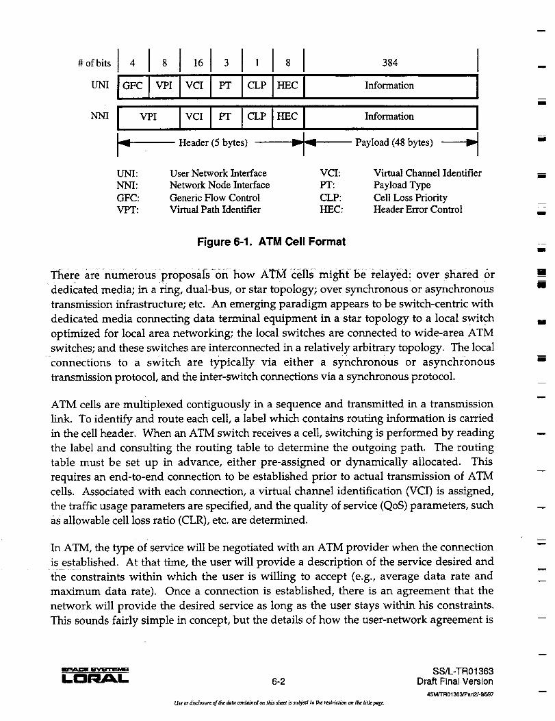
# of bits
UNI
NNI
4 ,i,6131,I,I
I_.., Header (5 bytes)I-
384
r]--_ Payload (48 bytes)
UNI: User Network Interface VCI:
NNI: Network Node Interface PT:
GFC: Generic Flow Control CLP:
VPT: Virtual Path Identifier HEC:
Virtual Channel Identifier
Payload Type
Cell Loss PriorityHeader Error Control
m
m
J
I
zI
Figure 6-1. ATM Cell Format
There are =numerous propoSals-0n how ATM Cells =migh( be relayedi over shared or
dedicated media; in a ring, dual-bus, or star topology; over synchronous or asynchronous
transmission infrastructure; etc. An emerging paradigm appears to be switch-centric with
dedicated media connecting data terminal equipment in a star topology to a local switch
optimized for local area networking; the local switches are connected to wide-area ATM
switches; and these switches are interconnected in a relatively arbitrary topology. The local
connections to a switch are typically via either a synchronous or asynchronous
transmission protocol, and the inter-switch connections via a synchronous protocol.
ATM ceils are multiplexed contiguously in a sequence and transmitted in a transmission
link. To identify and route each cell, a label which contains routing information is carried
in the cell header. When an ATM switch receives a cell, switching is performed by reading
the label and consulting the routing table to determine the outgoing path. The routing
table must be set up in advance, either pre-assigned or dynamically allocated. This
requires an end-to-end connection to be established prior to actual transmission of ATM
cells. Associated with each connection, a virtual channel identification (VCI) is assigned,
the traffic usage parameters are specified, and the quality of service (QoS) parameters, such
as allowable cell loss ratio (CLR), etc. are determined.
In ATM, the type of service will be negotiated with an ATM provider when the connection
is established. At that time, the user will provide a description of the service desired and
the constraints within which the user is willing to accept (e.g., average data rate and
maximum data rate). Once a connection is established, there is an agreement that the
network will provide the desired service as long as the user stays within his constraints.
This sounds fairly simple in concept, but the details of how the user-network agreement is
m
[]
m
I
m
m
w
I-Dl'_a_,l,, 6-2
Use or disclosure of the data contained on this sh_ is subject to the restriction on the title page.
SS/L-TR01363Draft Final Version
45M/TR01363/Pa rt2/-gFu,_7

=¸;::¸7
reached, what happens if any of the parties fail to live up to their end of the agreement,
how agreements are coordinated across possibly many switches, how the switch can help
shape terminal traffic, etc. are complex, numerous, and contentious. The ATM Forum, in
its User-Network Interface (UNI) specification, has taken the first steps in providing some
definitions in this area, but there is a great deal more to do.
6.1.1 ATM Service Categories
The ATM Forum currently defines five service categories [40]:
(1) Constant Bit Rate (CBR),
(2) Real-Time Variable Bit Rate (rt-VBR),
(3) Non-Real-Time Variable Bit Rate (nrt-VBR),
(4) Available Bit Rate (ABR), and
(5) Unspecified Bit Rate (UBR)
ATM service categories may be arranged into two groups: those supporting real-time
applications and those which do not. Real-time service classes are CBR and rt-VBR. The
non-real-time service classes are nrt-VBR, ABR, and L_R. Table 6-1 provides the attributes
of the ATM service categories [41].
Table 6-1. Attributes of ATM Traffic Categories
H_
w
L_
.,.j.
Service
Category
CBR
rt-VBR
nrt-VBR
ABR
UBR
Typical TrafficType
Voice or video
Image or
compressedvideo
Data
Data
(email, fax,
file transfer)
Cell
SwitchingPriority
High
Medium
Low
Low
Bit Rate
Constant
Bursty
Bursty
Bursty
DelaySensitivity
Yes
Yes
No
No
No
TargetCLR
for CLP=0
1.7 E-10
1.0 E-7
1.0 E-7
No target
glla,_ld_lE BYtC'rI_MII3
6-3
Use or disclosure of lhe data contained on this sheet is subject to the restriction on the title page.
SS/L-TR01363Draft Final Version
45M/TR01363/Pa rt2/- _a/E/
6.1.1.1 Constant Bit Rate
The CBR service supports leased line connections and real-time applications such as voice
and video by providing end-to-end timing recovery. The traffic can be characterized by a
constant cell arrival rate, which corresponds to a peak cell rate (PCR), and therefore, it
requires a predefined dedicated capacity equivalent to its PCR. Cells conforming to this
traffic pattern are guaranteed a QoS. A CBR contract typically specifies the cell loss ratio
(CLR), cell delay variation (CDV), and maximum cell transfer delay (CTD) as the QoS
parameters.
6.1.1.2 Variable Bit Rate
The VBR service supports bursty applications which can benefit from statistical
multiplexing. Based on traffic delay requirements, the VBR service is further divided into
two sub-categories, referred to as rt-VBR and nrt-VBR. The rt-VBR service is intended for
real-time applications with variable bit rate such as packetized voice and video
applications. The nrt-VBR service is intended for non-real-time applications such as data
services. In contrast to CBR, where a constant amount of capacity equivalent to PCR is pre-
reserved, VBR requires an average capacity which is equal to the sustainable cell rate
(SCR). The rt-VBR traffic contract specifies an acceptable CLR, CTD as well as CDV.
Compared to the CBR and rt-VBR service categories, the nrt-VBR category does not place
stringent requirements on the network for CDV and CTD, and only a mean CTD is
ensured.
6.1.1.3 Available Bit Rate
Similar to nrt-VBR, the ABR service category is suitable for data applications such as e-
mail, fax transmission, file transfers, and Telnet. The main difference is a guarantee for a
minimum throughput, known as minimum cell rate (MCR), as opposed to the VBR's
average cell rate SCR. In addition, the ABR service is designed to support applications
which cannot effectively characterize their traffic behavior at connection establishment but
can adapt their traffic following a feedback flow control protocol. For example, ABR
transmission rates may be reduced due to a congestion indication from the network. In the
ABR service, if the source behaves in a certain way in response to feedback flow control,
then no packets will be intentionally dropped.
6.1.1.4 Unspecified Bit Rate
The UBR service category is intended for applications which are tolerant to delay and do
not require non-real-time response. Furthermore, no guarantees on the CLR are offered,
thus leaving it to the end-system applications to handle. With this service, the user is
willing to tolerate whatever capacity and cell loss the network can provide at the instant
the cell goes through the network. Therefore, UBR is ideally suited to low-cost and low-
priority services such as electronic mail or low-tariff file transfers. Practically, large buffers
are used to minimize cell loss at the expense of delay.
= =m
=_
mm
BI
Zm
BB
=
U
H
lib
iW
mw
W_
LlCi_L 6-4
Use or disclosure of the data contained on this sheet is sub_ect to the restriction on the title page.
SS/L.-TR01363
Draft Final Version
45M/TR01363JPar12/-9_97

w
w
w
L Jm
M
= ,
u
w
w
6.1.2 ATM Adaptation Layer
To support the multiplicity of user information within a common ATM cell structure, the
ATM adaptation layer (AAL) is defined for five classes of user information:
(1) Type 1: intended to provide connection-oriented, CBR traffic.
(2) Type 2: intended to provide connection-oriented, rt-VBR traffic.
(3) Type 3/4: intended to provide connection-oriented and connection_less, nrt-VBR,
ABR, and UBR traffic.
(4) Type 5: This protocol grew out of concerns about the complexity for Type 3/4. Its
original name was Simple and Efficient AAL (SEAL), and it performs a subset of
AAL Type 3/4 functions.
The primary purpose of the AAL is to map user information into ATM cells in the most
suitable form for a desired application. The AAL functions include segmentation,
reassembly, sequence numbering, error protection, and transmission of timing information.
6.1.3 ATM Layer
The ATM layer provides for the transparent transfer of ATM service data units (SDU) over
already existing virtual circuits among communicating users. All ATM SDUs are simply 48
bytes of data. The functions performed by the ATM layer include:
(1) Multiplexing of ATM connections
(2) Cell relay and routing
(3) Cell delineation
(4) Payload type discrimination
(5) Selective cell discarding
(6) Cell rate shaping
(7) Enforcement of traffic contract.
6.1.4 Physical layer
The physical layer provides ATM cells transportation services to the ATM layer. It consists
of two sublayers: the Physical Medium (PM) sublayer and the Transmission Convergence
(TC) sublayer. The PM sublayer performs physical medium dependent functions such as
specifying the physical medium, the transmission characteristics, and the insertion and
extraction of timing information. The TC sublayer performs cell delineation, cell rate
decoupling, Header Error Check (HEC) generation and verification, and mapping the cells
received from the ATM layer into frames of the transmission system. The HEC field is
used for cell header single-bit-error correction and multiple-bit-error detection. Cells with
uncorrectable errors in the cell header are discarded.
m HVIFrIg_WS
LDRb_,L. 6-5
Use or disclosure of the data contained an this sh_t is subject to the restriction on the tith_ page.
SS/L-TR01363Draft Final Version
45 M/TRO 1363_a r_J'- 9_97

Currently, there are two major groupings of physical layer protocols for ATM:
(1) Based on Plesiochronous Digital Hierarchy (PDH)
(2) Based on Synchronous Digital Hierarchy (SDH).
PDH is basically the existing digital telephony transmission system. There are five levels in
the PDH, though the bit rates associated with these levels vary with geological region. In
the U.S., the levels of the hierarchy are DS-0 (64 kbit/s), DS-1 (1.544 Mbit/s), DS-2 (6.312
Mbit/s), DS-3 (44.736 Mbit/s), and DS-4 (139 Mbit/s). The ATM Forum has defined a way
for the DS-1 and DS-3 framing structures to carry ATM cells.
SDH is a flexible synchronous time division multiplexing transmission system defined by
the ITU-T to carry data streams at rates higher than those defined in PDH. SDH was
derived from Synchronous Optical Network (SONET). SONET defines a set of framing
formats, transmission speeds, and multiplexing standards. The first level of the SONET
framing hierarchy is STS-1 (51.84 Mbit/s). When the STS-1 structure is carried over fiber
optic medium, the resulting service is called OC-1. Higher synchronous rates (STS-N) are
achieved by multiplying the basic rate by N (e.g., OC-3 (155.52 Mbit/s), OC-12 (622.08
Mbit/s), OC-48 (2488.37 Mbit/s)). To transport ATM cell streams over SDH/SONET, the
TC sublayer performs the mapping of the ATM cell into the SDH/SONET frames. All
timing and synchronization functions are performed by the SDH/SONET transmission
systems.
6.1.5 ATM Traffic Management
The ATM layer defines a comprehensive set of ATM service categories controlled by a
sophisticated set of traffic management functions and procedures. The challenge is to
balance a high quality service with maximum network utilization. For example, a low
network utilization is expected if capacity is reserved for PCRs of every connection to
achieve a high service quality. This option is uneconomical to operate because all
connections do not continually operate at full capacity. Another option is to allocate
resources in a way in which there are always more connections than available capacity. In
this case, the network utilization will be high, but the QoS will be unacceptable during
peak usage periods. Therefore, effective traffic management requires end-to-end
participation of all network elements. Traffic management functions and procedures at an
ATM node are typically distributed among interface modules, switch fabric, and a control
module. The four traffic management building blocks are:
(1) Traffic parameter descriptors,
(2) Quality of Service parameters,
(3) Connection admission control (CAC),
(4) Conformance monitoring and enforcement, and
(5) Congestion control.
= =
u
mmk
u
[]
ml
[]N
Hmml
u
i
LD L 6-6
Use or disclosure of the da ha con tained on this sheet is sx_ect to the restriction on the title page.
SS/L-TR01363Draft Final Version
45MJTR01363JP a rt2/- 9F_37
w
u

= :
w
w
! -
! •
6.1.5.1 Traffic Parameter Descriptors
A traffic descriptor defines the bandwidth guidelines to which a connection within a
service category must adhere. Traffic descriptors are required to ensure proper resource
allocation and guarantee the QoS across an ATM network. A traffic descriptor has two key
elements: Source Traffic Descriptor and Cell Delay Variation Tolerance (CDVT).
The Source Traffic Descriptor is a set of parameters which describes the expected
bandwidth utilization which the connection needs. These parameters are PCR, SCR and
Maximum Burst Size (MBS), and MCR. The set of traffic descriptors conveyed at
connection set up varies depending on the connection's service category. A sustained bi-
directional connection has a set of connection traffic descriptors for each direction. Note
that the descriptor sets need not be the same for each direction. Source traffic descriptors
can specify CLP_0 cell traffic, or the aggregate CLP_0+I traffic.
The CDVT is a network descriptor that provides a measure of the jitter in the cell inter-
departure pattern of a given connection. Jitter is typically caused by the multiplexing effect
of placing several virtual circuits on a single connection.
6.1.5.2 Quality of Service Parameters
ATM QoS is measured and specified in terms of the following parameters:
(1) Cell Delay Variation (CDV),
(2) Maximum Cell Transfer Delay (Max CTD),
(3) Cell Loss Ratio (CLR),
(4) Cell Error Ratio (CER),
(5) Severely Errored Cell Block Ratio (SECBR), and
(6) Cell Misinsertion Rate (CMR).
Of these six QoS parameters, only CDV, max CTD, and CLR are specified on a per-
connection basis. CER, CMR, and SECBR take default values which the network
guarantees to meet for all connections. Specification of individual QoS parameters is
currently supported by the ATMF UNI Signaling 4.0. In addition, the ATMF LTNI Signaling
4.0 provides mechanisms for the negotiation of CDV, max CTD, and CLR between the user
and the network.
The traffic descriptors and QoS parameters are the main components of a traffic contract
representing a mutual agreement between the user and the network provider. The user
specifies its connection descriptors and a set of QoS parameters in each direction, and the
network agrees to provide the QoS level specified in this contract.
w
L
I..1I:3_1. 6-7
Use or disclosure of tht data contained on this sheet is subject to the restriction on tht title page.
SS/L-TR01363Draft Final Version
45 M/TR01363JPa rt2/- 9FJ37

6.1.5.3 Connection Admission Control
Connection Admission Control (CAC) is the set of actions taken by the network during the
connection set-up phase in order to determine whether a connection request can be
accepted or denied, and to ensure that existing connections are not affected when a new
one is established. CAC involves determining the bandwidth/capacity required by each
connection along the path to support the traffic descriptors and the QoS requirements
included in the traffic contract. If a connection request is accepted, the network allocates
certain bandwidth capacity to the connection. The end-systems and all intermediate ATM
nodes are active participants of CAC. Each node along the path can reject the connection
request if it can not meet the defined QoS parameters.
The set of traffic descriptors and QoS parameters indicated for a connection request
depends on the ATM service category. Therefore, the computation of the required
bandwidth is different for each category. The simplest CAC algorithm allocates bandwidth
equivalent to the PCR for each connection. Although this is appropriate for CBR
connections, it proves to be overly conservative for VBR connections. Service providers can
take advantage of significant statistical multiplexing gains in VBR using the lower SCR
parameter, rather than PCR. Service providers prefer powerful CAC algorithms which
take into account SCR, as well as PCR, for accepting or refusing a connection request. This
optimizes utilization of network resources for VBR traffic and ensures that the network
meets the required QoS of the new connection, as well as maintaining the agreed QoS of
the existing connection.
For CAC to be credible, the algorithm needs to factor in all of the standard traffic
descriptors. In addition, a unique algorithm is required for _each of the five service
categories: CBR, rt-VBR, nrt-VBR, ABR and UBR. Ensuring that each of these algorithms is
optimal will result in efficient allocation of network bandwidth. Thus, how refined these
algorithms are will determine how efficiently bandwidth is allocated.
6.1.5.4 Conformance Monitoring and Enforcement
When a network carries an ATM connection, it commits to provide the agreed QoS to all
the ceils conforming to the theoretical generic cell rate algorithm (GCRA). The GCRA has
been selected by both the ITU-T Recommendation 1.371 and ATM TM 4.0 specification to
define conformance with respect to the source traffic descriptors and the CDVT. To
achieve this objective, the network polices the traffic of the connection to detect non-
conforming ceils, and takes appropriate action on these cells to prevent them from affecting
the QoS of the conforming cells of other connections. The compliance enforcement is done
by a Usage Parameter Control (UPC) process at the UNI and optionally by a Network
Parameter Control (NPC) process at the NNI (Network-to-Network Interface).
U
I
I
I
m
L_
B
M
mw
w
l,.O_[.. 6-8
Use or disclosure of the data contained on this sheet is subject to the restriction on the title page.
SS/L-TR01363Draft Final Version
45M/TR01363/PaP_./- _FJ7
u
romE

w
w
= ,
r
w
g
The CAC and UPC/NPC functions must work together to protect the network from
congestion while meeting the network performance objectives of all current connections.
The CAC uses the traffic descriptors of the connections to allocate bandwidth/capacity,
while the UPC/NPC polices the network connections, making sure the traffic conforms to
the traffic descriptors. In this way, users are isolated from one another, and are not affected
by any "misbehaving" users.
A UPC/NPC process implements one or more leaky bucket algorithms to police each
connection. Each leaky bucket mechanism has two parameters: the increment parameter
corresponds to the inverse of the compliant rate (fill rate of the bucket) and the limit
parameter corresponds to the number of cells that can burst at a higher rate (size of the
bucket). When more than one traffic descriptor is used (for example, PCR and SCR) for a
connection, multiple leaky buckets are cascaded, with the highest rate being policed first.
For example, ATM connections carrying frame relay service may actually define three
traffic descriptors and thus require three leaky buckets: PCR0, PCR1 and SCR0.
6.1.5.5 Congestion Control
There are two general categories of congestion control: preventive control and reactive
control. As indicated by their names, a preventive control technique prevents congestion
by taking appropriate actions before it actually occurs. In a reactive control technique, the
network is monitored for congestion. When congestion is detected, sources are requested
to slow down or stop transmission until the end of congestion.
Early Packet Discard (EPD) and Partial Packet Discard (PPD) are preventive congestion
examples. A network can quickly experience a state of congestion as increasing levels of
cell loss generate more and more packet re-transmission requests. EPD fixes the problem
of flooding the network with re-transmissions by discarding cells on a packet level rather
than a cell level. This drastically reduces useless traffic caused by the transfer of corrupted
data packets which have to be re-transmitted by the sender. EPD and PPD are applied to
ABR and UBR traffic of AAL Type 5 connections, which are used especially for this packet
traffic.
Feedback flow control mechanisms are considered reactive control techniques which can be
used to guarantee the QoS of existing connections in case network capacities run low. The
objective is to reduce the overall traffic in a way that the network never reaches an
undesirable state of congestion. As mentioned previously, the ATM network informs the
traffic sources of impending congestion; on receiving this information, the traffic sources
stop increasing or slow down their traffic. Table 6-2 indicates that implementation of a
feedback flow control mechanism is mandatory for the ABR service category and optional
for the other services. Section 6.2 provides a summary of several feedback flow control
mechanisms.
m
N_
LDr'_Jc_L 6-9
Use or disclosure o_ the data contained on this sheet is subject to the restriction an the title page.
SS/L-TR01363Draft Final Version
45 M/TR01363_ ar t2/- _-'J_'
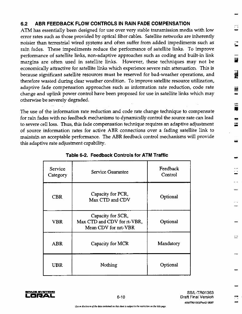
6.2 ABR FEEDBACK FLOW CONTROLS IN RAIN FADE COMPENSATION
ATM has essentially been designed for use over very stable transmission media with low
error rates such as those provided by optical fiber cables. Satellite networks are inherently
noisier than terrestrial wired systems and often suffer from added impediments such as
rain fades. These impediments reduce the performance of satellite links. To improve
performance of satellite links, non-adaptive approaches such as coding and built-in link
margins are often used in satellite links. However, these techniques may not be
economically attractive for satellite links which experience severe rain attenuation. This is
because significant satellite resources must be reserved for bad-weather operations, and
therefore wasted during clear weather condition. To improve satellite resource utilization,
adaptive fade compensation approaches such as information rate reduction, code rate
change and uplink power control have been proposed for use in satellite links which may
otherwise be severely degraded.
The use of the information rate reduction and code rate change technique to compensate
for rain fades with no feedback mechanisms to dynamically control the source rate can lead
to severe cell loss. Thus, this fade compensation technique requires an adaptive adjustment
of source information rates for active ABR connections over a fading satellite link to
maintain an acceptable performance. The ABR feedback control mechanisms will provide
this adaptive rate adjustment capability.
Table 6-2. Feedback Controls for ATM Traffic
"ill
[]u
I
==
I
m
It
m
L_
BB
_m
am
u
Service
Category
CBR
VBR
UBR
Service Guarantee
Capacity for PCR,Max CTD and CDV
Capacity for SCR,
Max CTD and CDV for rt-VBR,
Mean CDV for nrt-VBR
Capacity for MCR
Nothing
Feedback
Control
Optional
Optional
Mandatory
Optional
g
:: =m
K.DI'_A_I- 6-10
Use or disclosure of the data contained on this sheet is subject to the restriction on the title page.
SS/L-TR01363DraftFinal Version
45M/TR01363/Part2/- _F_97
==i
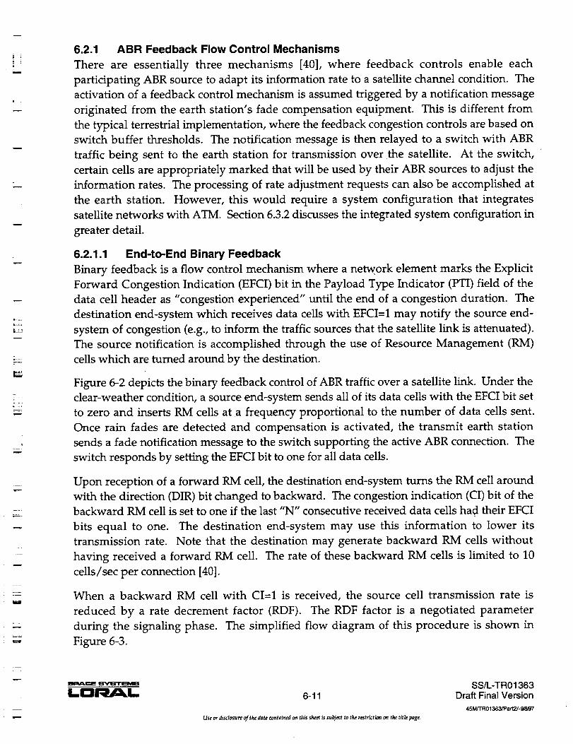
w
=....
k_a
I
r_
6.2.1 ABR Feedback Flow Control Mechanisms
There are essentially three mechanisms [40], where feedback controls enable each
participating ABR source to adapt its information rate to a satellite channel condition. The
activation of a feedback control mechanism is assumed triggered by a notification message
originated from the earth station's fade compensation equipment. This is different from
the typical terrestrial implementation, where the feedback congestion controls are based on
switch buffer thresholds. The notification message is then relayed to a switch with ABR
traffic being sent to the earth station for transmission over the satellite. At the switch,
certain ceils are appropriately marked that will be used by their ABR sources to adjust the
information rates. The processing of rate adjustment requests can also be accomplished at
the earth station. However, this would require a system configuration that integrates
satellite networks with ATM. Section 6.3.2 discusses the integrated system configuration in
greater detail.
6.2.1.1 End-to-End Binary Feedback
Binary feedback is a flow control mechanism where a network element marks the Explicit
Forward Congestion Indication (EFCI) bit in the Payload Type Indicator (PTI) field of the
data cell header as "congestion experienced" until the end of a congestion duration. The
destination end-system which receives data cells with EFCI=I may notify the source end-
system of congestion (e.g., to inform the traffic sources that the satellite link is attenuated).
The source notification is accomplished through the use of Resource Management (RM)
cells which are turned around by the destination.
Figure 6-2 depicts the binary feedback control of ABR traffic over a satellite link. Under the
clear-weather condition, a source end-system sends all of its data cells with the EFCI bit set
to zero and inserts RM cells at a frequency proportional to the number of data cells sent.
Once rain fades are detected and compensation is activated, the transmit earth station
sends a fade notification message to the switch supporting the active ABR connection. The
switch responds by setting the EFCI bit to one for all data cells.
Upon reception of a forward RM cell, the destination end-system turns the RM cell around
with the direction (DIR) bit changed to backward. The congestion indication (CI) bit of the
backward RM cell is set to one if the last "N" consecutive received data cells had their EFCI
bits equal to one. The destination end-system may use this information to lower its
transmission rate. Note that the destination may generate backward RM cells without
having received a forward RM cell. The rate of these backward RM cells is limited to 10
cells/sec per connection [40].
When a backward RM cell with CI=I is received, the source cell transmission rate is
reduced by a rate decrement factor (RDF). The RDF factor is a negotiated parameter
during the signaling phase. The simplified flow diagram of this procedure is shown in
Figure 6-3.
LD_L 6-11
Use or disclosure of the data contained on this sheet is subject to the restriction on the title page.
SS/L-TR01363Draft Final Version

E 3-ts3fade notificationr.Al_rn /
Satellite
_j
n
/
[-_ Data Cell with EFCI=! D Data Cell with EFCI=0 [_RM Cell
Figure 6-2. End-to-End Binary Feedback Flow Control
h
u
j
SOURCECells (data and RM)
CI= 1: Reduce ceil sending rate graduallyNI=I: Do not increase ce]l sending rate
Cl=0 & NI=0: Increase cell sending rate gradually
/Yes (i.e., data cells) I
, ATM Switch
RM cells)
i
If FadingSET
PT--01x
DESTINATION:
1. EXAMINE DATA CELLS2. IF PT=01x THEN
3. MODIFY RM CELLS BY SETTING
CI=I4. TURN RM CELLS AROUND TO SOURCE
Backward RMs
w
r
Figure 6-3. Simplified Flow Diagram of End-to-End Binary Feedback Control
N UPII_R'IEaMB
6-12
Use or discl_ure of the data contained on this sheet is subject to the restriction on the title page.
SS/L-TR01363Draft Final Version
45M/TR01363/Part2/- 9E_J7n
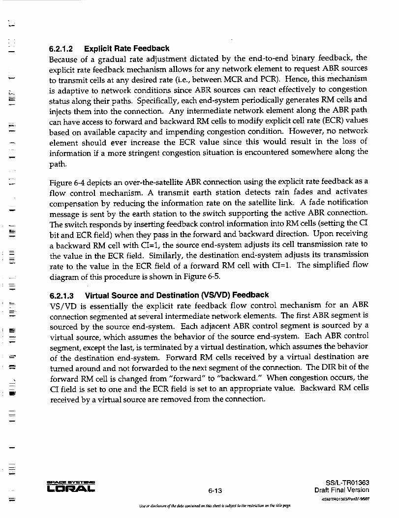
w
w
w
F
.=,
m
=
BIB$
6.2.1.2 Explicit Rate Feedback
Because of a gradual rate adjustment dictated by the end-to-end binary feedback, the
explicit rate feedback mechanism allows for any network element to request ABR sources
to transmit cells at any desired rate (i.e., between MCR and PCR). Hence, this mechanism
is adaptive to network conditions since ABR sources can react effectively to congestion
status along their paths' Specifically, each end-system periodically generates RM cells and
injects them into the connection. Any intermediate network element along the ABR path
can have access to forward and backward RM cells to modify explicit cell rate (ECR) values
based on available capacity and impending congestion condition. However, no network
element should ever increase the ECR value since this would result in the loss of
information if a more stringent congestion situation is encountered somewhere along the
path.
Figure 6-4 depicts an over-the'satellite ABR connection using the explicit rate feedback as a
flow control mechanism. A transmit earth station detects rain fades and activates
compensation by reducing the information rate on the satellite link. A fade notification
message is sent by the earth station to the switch supporting the active ABR connection.
The switch responds by inserting feedback control information into RM cells (setting the CI
bit and ECR field) when they pass in the forward and backward direction. Upon receiving
a backward RM cell with CI=I, the source end-system adjusts its cell transmission rate to
the value in the ECR field. Similarly, the destination end-system adjusts its transmission
rate to the value in the ECR field of a forward RM cell with CI=I. The simplified flow
diagram of this procedure is shown in Figure 6-5.
6.2.1.3 Virtual Source and Destination (VS/VD) Feedback
VS/VD is essentially the explicit rate feedback flow control mechanism for an ABR
connection segmented at several intermediate network elements. The first ABR segment is
sourced by the source end-system. Each adjacent ABR control segment is sourced by a
virtual source, Which assumes the behavior of the source end-system. Each ABR control
segment, except the last, is terminated by a virtual destination, which assumes the behavior
of the destination end-system. Forward RM cells received by a virtual destination are
turned around and not forwarded to the next segment of the connection. The DIR bit of the
forward RM cell is changed from "forward" to "backward." When congestion occurs, the
CI field is set to one and the ECR field is set to an appropriate value. Backward RM cells
received by a virtual source are removed from the connection.
i.
RI_J=E
LDI'_,C_L 6-13
Use or discJosur¢ of the data contained on this sheet is subject to the restriction on the title page.
SS/L-TR01363Draft Final Version
45 M/TR 01363/PaR2J- _-u,_7
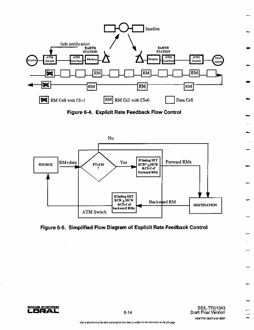
fade notification /EARTH
Satellite
]-----
['_] RM Cell with CI= l ['_RM Cell with CI--O --']Data Cell
Figure 6-4. Explicit Rate Feedback Flow Control
No
ATM Switch
If fading SET
ECR* >MCR&CI=I of
Forward RMs
/If fading SET |
ECR >MCR _ Backw&CI=I of
backward RMs
Forward RMs
]t' _'
DESTINATION
J
m
h
k
ira--.
= =
i
m
Figure 6-5. Simplified Flow Diagram of Explicit Rate Feedback Control
LI31"4/_L 6-14
Useor disclosurt of thedata containedon this shtt't is subject to thertstffctionon the tith',page.
SS/L-TR01363Draft _n_ Ve_on _
45M/I"RO1363/Part2/-_B7
m

w
m
w
•2 _]
Figure 6-6 depicts an over-the-satellite ABR connection using the VS/VD feedback as a
flow control mechanism. The ABR connection is divided into three separately controlled
ABR segments. The ATM Switch 1 becomes the virtual destination for the source end-
system, and the ATM Switch 2 becomes the vlrtual source for the destination end-system.
A transmit earth station detects rain fades and activates compensation by reducing the
information rate on the satellite link. The earth station then sends a fade notification
message to Switch 1. Upon receiving the notification message, Switch I modifies the CI bit
and ECR value for RM cells that are not terminated by Switch 1 (i.e., RM cells turned
around to the source end-system and RM cells transmitted over the satellite). Switch 2
examines the CI and ECR fields of RM cells coming from Switch 1 and sets RM cells
destined for the destination end-system accordingly. Upon receiving RM cells with CI=I,
the source and destination end-systems set the cell transmission rates equal to the value
specified in the ECR. The simplified flow diagram of this procedure is shown in Figure 6-7.
6.2.2 Assessments
Table 6-3 compares the feedback flow control mechanisms using criteria such as response
delay, cell rate adjustment method, and reliability. The response delay refers the elapsed
time beginning when the earth station decides to compensate for fading until the source
end-system of a particular ABR connection receives a "congestion notification" message.
The rate adjustment method criterion assesses a given feedback control mechanism to
request the transmission rates explicitly or relatively. The last criterion refers to the reliable
arrival of the congestion notification message at the source. An evaluation of the feedback
flow control mechanisms is provided in the following paragraphs.
_C)--_ Satellite
fade notification /
®
Figure 6-6. VSND Feedback Flow Control
IRl_=eM_m
6-15
Use or disclosure of the data contained on this sheet is sttbject to the restriction on lhe title page.
SS/L-TR01363Draft Final Version
45 M/I'R01363/Part2/-_16_7
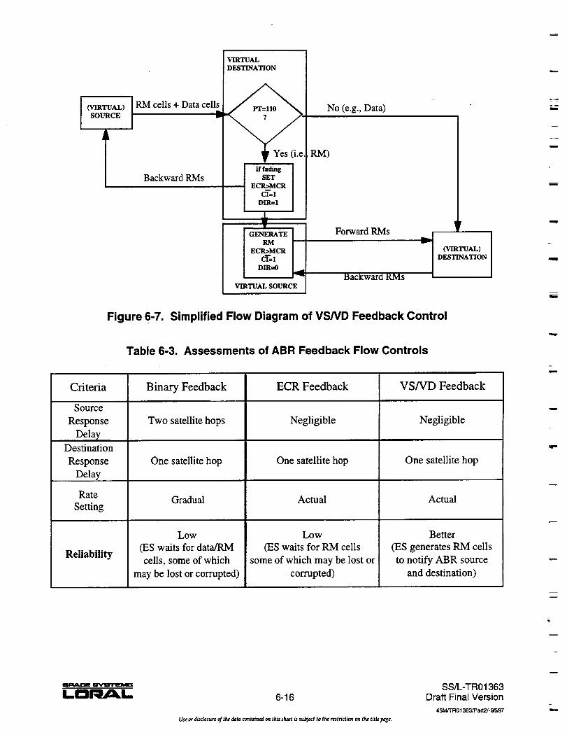
(VIRTUAL)SOURCE
TI RM cells + Data cells
Backward RMs
VIRTUAL
DESTINATION
SET
ECR>MCRcY--1
DIR=I
Y
]GENERATE]ECR>MCRc'T'= 1RMDm---o
VIRTUAL SOURCE
No (e.g., Data)
RM)
Forward RMs
Backward RMs
]r
(VIRTUAL)
DESTINATION
Figure 6-7. Simplified Flow Diagram of VSND Feedback Control
Table 6-3. Assessments of ABR Feedback Flow Controls
±=_
N
w
m
=
u
Criteria
Source
Response
Delay
Destination
Response
DelaY.r,.,
Rate
Setting
Reliability
Binary Feedback
Two satellite hops
One satellite hop
Gradual
Low
(ES waits for data/RM
cells, some of which
may be lost or corrupted)
ECR Feedback
Negligible
One satellite hop
Actual
Low
(ES waits for RM cells
some of which may be lost or
corrupted)
VS/VD Feedback
Negligible
One satellite hop
Actual
Better
(ES generates RM cells
to notify ABR source
and destination)
w
rw
i
1--Dl' O t- 6-16
Useor disclosureof thedata containedon thissheet is subject to the restriction on the title page.
SS/L-TR01363Draft Final Version
45M/TR01363/Part2J-_FJ37r
b

w
w
w
w
6.2.2.1 Response Delay
For the end-to-end binary feedback, the time it takes a data cell with EFCI=I to arrive at the
destination end-system from transmit earth station is a single satellite hop propagation
delay (approximately 240 ms). Delays due to processing and terrestrial propagation are
assumed negligible. If the destination reacts upon receiving this data cell, the source end-
system would receive a backward RM celI marked with CI=I one satellite delay later.
Therefore, the response delay of the end-to-end binary feedback is two satellite hop
propagation delays.
In the explicit rate feedback, the destination response delay is the same as the binary
feedback, as shown in Figure 6-2. However, the source is much faster in adapting its rate to
the current state of the link since the delay of backward RM cells from the transmit earth
station to source is insignificant.
Similar to the explicit rate feedback, the time to request an ABR source end-system to
transmit ceils at any desired rate is almost immediately. As shown in Figure 6-6, this is
accomplished by the turned-around RM ceils in the first loop of the ABR path. The delay
of feedback control information tO the destination end-system from the transmit earth
station is the same as the other two feedback mechanisms.
6.2.2.2 Rate Adjustment Method
As mentioned previously, the binary feedback control mechanism uses the gradual
transmission rate decrease approach. It is therefore not effective against short term fading
since rate reduction delays may exceed the fade duration. The explicit rate and VS/VD
feedback mechanisms however allow for the actual specification of desired transmission
rates on any ABR connections based on the satellite link capacity under different fading
conditions.
6.2.2.3 Reliability
The binary: feedback mechanism is less reliable since feedback control cells must
successfully propagate through the satellite twice before reaching the source end-system.
The explicit rate feedback control mechanism is more reliable than the binary feedback, but
backward RM cells transported by a faded return satellite link must survive. The VS/VD
feedback mechanism therefore appears to be more favorable, since the source end-system
adjusts its transmission rate based on information contained in feedback control ceils
transported by a terrestrial link in the first loop (i.e., not transported by the satellite link
experiencing rain fades).
LD_L 6-17
Use or disclosure of the data contained on this sheet is subject to the restriction on the title page.
SS/L-TRO 1363Draft Final Version
45 M/TR01363]Pa rt2J-9F_97

=
m
6.2.2.4 Recommendation
Practical considerations play an important part in implementing a given feedback
mechanism in satellite networks, where the propagation delays are large compared to
terrestrial networks. From the above discussions, the end-to-end binary feedback
mechanism is unacceptable due to its long source response delay and gradual transmission
rate decrease approach. The explicit rate feedback mechanism is acceptable from the
viewpoint of its response delay and explicit rate specification. However, since this
mechanism depends on the arrival of backward RM cells in a critical time, it is not reliable
while the satellite link is degraded. Similar to the explicit rate feedback, the VS/VD
feedback mechanism accomplishes a negligible response delay and explicit rate
transmission request. It is superior to the explicit rate feedback for the ability that the
request to reduce source transmission rate is reliably transmitted to the source via
terrestrial links and that the request can be generated by the source's virtual destination.
6.3 SYSTEM CONFIGURATION FOR IMPLEMENTING FADE COMPENSATION
COMSAT Laboratories manufactures an ATM Link Accelerator TM, model ALA-2000 TM [42],
which facilitates the transmission of ATM traffic over satellite systems. The ALAs perform
rate adaptation and signal conditioning functions to output data at rates of up to 8.448
Mbit/s but do not implement any of the ABR feedback flow control mechanisms. As
shown in Figure 6-8, modified versions of ALA-2000 units will be required. The ABR
sources are connected to the switches through physical links running at standard rates such
as 51.84 Mbit/s over OC-1 lines. The switches are interconnected via links running at
155.52 Mbit/s (STS-3). The ALAs are connected to the switches via links running at 44.736
Mbit/s over DS-3 lines. Another possible system configuration would make use of the
interface proposed in [43].
ABR source
ABR source
ABR source
Standard Rates
El, DS1, DS3 ....
MODEM
MODEM
MODEM
Figure 6-8. System Configuration for Implementing Fade Compensation
r_
u
i
_I
I
lip
i
[]
m
w
V
rlu
i
6-18
Use or disclosure of the data contained on this sheet is subject to the restriction on the title page.
SS/L-TR01363Draft Final Version
45M/'rR01_3/Part2/-0_a_d'/

. J
=--
_=_
m
L_
_m
SECTION 7 -- SYSTEM REQUIREMENTS
In order for the selected fade mitigation schemes to operate successfully consideration
must be given to several system related aspects. These include system margin, setup time
required to invoke the mitigation scheme, fade compensation range, and size of the
common resource pool required for fade compensation. Most of these issues cannot be
addressed adequately without defining the overall system requirements. An outline of a
general approach to selecting the system parameters that affect fade mitigation is given
below.
7.1 SYSTEM MARGIN
System margin is directly related to the service availability requirements. This in turn is
largely a function of the rain climate in which the service is to be provided and the
elevation angle. When implementing fade mitigation the system margin may be considered
in terms of a fixed component and a dynamic component. The fixed allocation essentially
takes care of the clear-sky conditions and the dynamic margin is the portion available
through the fade compensation schemes being implemented. The clear-sky margin must
allow for clear-air signal attenuation, measurement inaccuracies associated with the link
quality measurement, and the time required for invoking the fade compensation.
Link quality estimation was discussed in Section 6 and typical measurement errors
associated with different measurement techniques were presented. Some of the techniques
pertain to measuring the link quality at one frequency (up-link or down-link) and scaling
this value to the other frequency. In this approach, errors are introduced in the frequency
scaling process and this must be factored into the clear-sky margin. Figure 7-1 shows
statistical behavior of frequency scaling from the down-link to the up-link. In this figure
the fade ratio between the up- and down-link fade is plotted against the down-link fade;
the results have been derived from ACTS beacon measurements at Clarksburg, MD. It is
seen that the estimation error is proportional to the down-link fade and for down-link
fades around 5 dB the estimation error is of the order of +0.5 dB. Most compensation
techniques have some overheads associated with them (signaling delays). During the time
period allocated for the overhead the link must stay intact, and to ensure this an
appropriate margin must be allowed. Assuming a fade rate of 0.5 dB/s and an overhead
of 2 s, the additional margin required is I dB. Another factor that must be accounted for in
applying fade compensation is the time duration for which the compensation is invoked.
The time duration must be significantly larger than the time associated with the overhead
to ensure adequate utilization of resources. This can be handled by including an
implementation margin of around 0.5 dB together with a suitable wait time after the fade
has ceased. The implementation margi n provides a hysteresis around the clear-sky
threshold to avoid very short duration fades which may cause the fade compensation to
LDI'_M_I,. 7-1
Use or disclosure of _he data contained on this sheet is subject to the restriction on the title page.
SS/L-TR01363Draft Final Version
45 M/TR01363/Pa r t2/- 9F._97
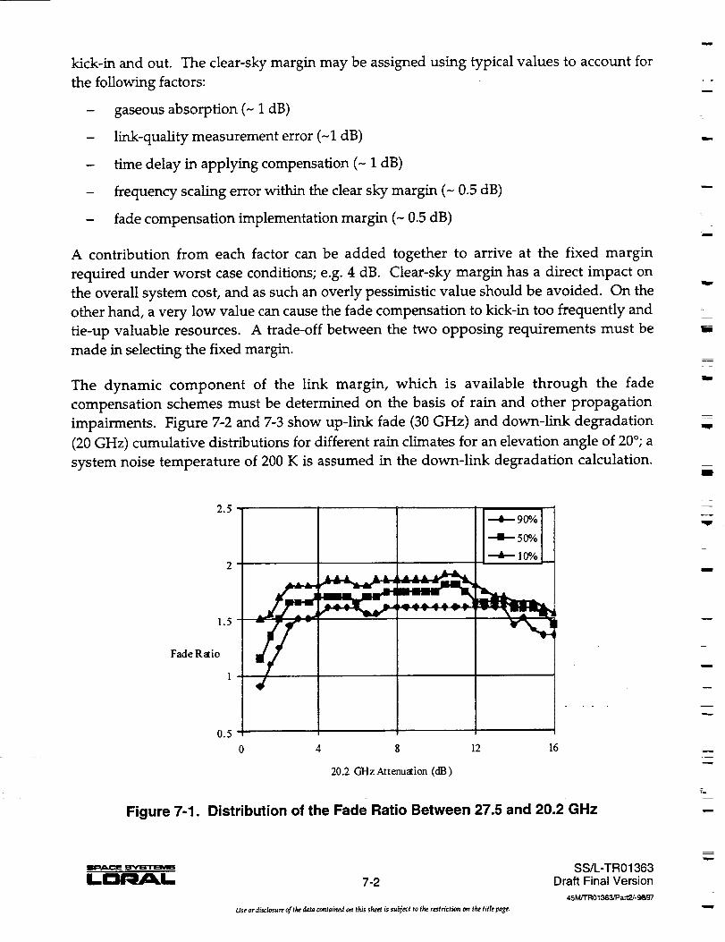
kick-in and out. The clear-sky margin may be assigned using typical values to account for
the following factors:
- gaseous absorption (- 1 dB)
- link-quality measurement error (-1 dB)
- time delay in applying compensation (- 1 dB)
- frequency scaling error within the clear sky margin (- 0.5 dB)
- fade compensation implementation margin (- 0.5 dB)
A contribution from each factor can be added together to arrive at the fixed margin
required under worst case conditions; e.g. 4 dB. Clear-sky margin has a direct impact on
the overall system cost, and as such an overly pessimistic value should be avoided. On the
other hand, a very low value can cause the fade compensation to kick-in too frequently and
tie-up valuable resources. A trade-off between the two opposing requirements must be
made in selecting the fixed margin.
The dynamic component of the link margin, which is available through the fade
compensation schemes must be determined on the basis of rain and other propagation
impairments. Figure 7-2 and 7-3 show up-link fade (30 GHz) and down-link degradation
(20 GHz) cumulative distributions for different rain climates for an elevation angle of 20°; a
system noise temperature of 200 K is assumed in the down-link degradation calculation.
u
b
y ±m
w
.I
W
m
m
1.5
Fade Raio
1
Figure 7-1.
0 4 8 12 16
20.2 GHz Attenuation (dB)
Distribution of the Fade Ratio Between 27.5 and 20.2 GHz
w
m
.m
w
LC:U_M_L 7-2
Use or disclosure of the data contained on this sheet is subject to the restriction on the title page.
SS/L-TR01363
Draft Final Version
45M/TR01363/Part2/-9_97
w

= =
r
_Z
50 -,.(_ ....
45 -'. _ .-: ....
40 _ iN \\
' _J III
35
30 "_ , _ : ",d ;IN' I%111
_25 _ i ! .1"___1_o_ _ >-LIII:
• II1"11
051 1 Ill.l "_ "_"("t'H.-k
0.01
Up-Lin k Atten u ation
,, IIIII\ IIIII
IIIII_ iili
_ Illl_;,,, _li
_ _ .._1 "-rT'_
1"1111'
0,1
l ....II111IIIIIIIII1
rJIll' IIIII
fi!!J
PercentTimeOrdinateExceeded
IIIII
IO
I
i
i
100
RainZone
--.4b--B
---B-D_F+H+K
-.Q---M i
Figure 7-2. Attenuation Distributions at 30 GHz for Different
Rain Zones; Elevation Angle 20 °
w
50
45
40
35
30
Downlirk 25
De gradation (dB)20
15
10
5
\ IIIIN %.1111
"_ _tll_'_ II1_
"_ x,,I III
II1:0
3.01 O.
Down-Lin k Degradation
IIIIIIIIIIII
IIIIIIIIIIII
IIIIII
. IIII IIII I r\ IIII Jill I
10
PercentTime Ordinate Exceeded
Rain Zone
...,4b.--B
•--g--D
_F_H
_K
_M
--.4..--P
100
_J'7
Figure 7-3. Down-Link Degradation Distributions at 20 GHz for Different
Rain Zones; Elevation Angle 20 °
LaI'_L 7-3
Use or disclosure qf the data contained on this sheet is subject to the restriction on the title page.
SS/L-TR01363Draft Final Version
45M/TR01363/Part_- 9_97
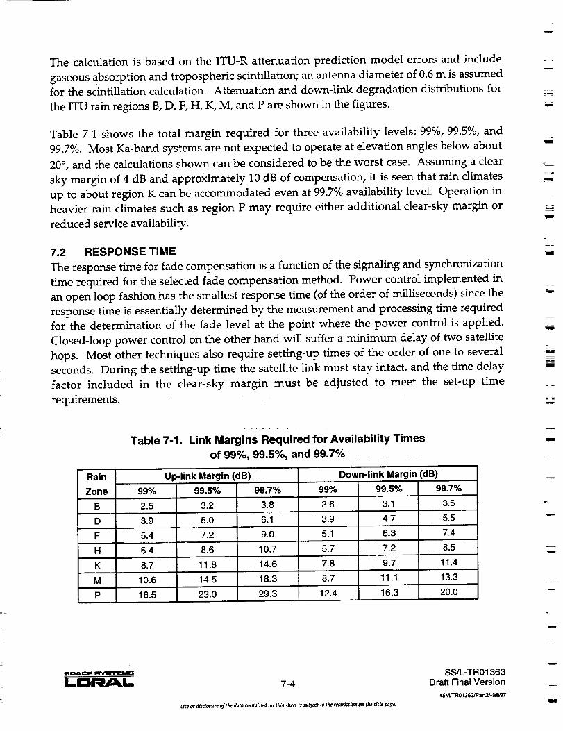
The calculation is based on the ITU-R attenuation prediction model errors and include
gaseous absorption and tropospheric scintillation; an antenna diameter of 0.6 m is assumed
for the scintillation calculation. Attenuation and down-link degradation distributions for
the ITU rain regions B, D, F, H, K, M, and P are shown in the figures.
Table 7-1 shows the total margin required for three availability levels; 99%, 99.5%, and
99.7%. Most Ka-band systems are not expected to operate at elevation angles below about
20 °, and the calculations shown can be considered to be the worst case. Assuming a clear
sky margin of 4 dB and approximately 10 dB of compensation, it is seen that rain climates
up to about region K can be accommodated even at 99.7% availability level. Operation in
heavier rain climates such as region P may require either additional clear-sky margin or
reduced service availability.
7.2 RESPONSE TIME
The response time for fade compensation is a function of the signaling and synchronization
time required for the selected fade compensation method. Power control implemented in
an open loop fashion has the smallest response time (of the order of milliseconds) since the
response time is essentially determined by the measurement and processing time required
for the determination of the fade level at the point where the power control is applied.
Closed-loop power control on the other hand will suffer a minimum delay of two satellite
hops. Most other techniques also require setting-up times of the order of one to several
seconds. During the setting-up time the satellite link must stay intact, and the time delay
factor included in the clear-sky margin must be adjusted to meet the set-up time
requirements.
Rain
Zone
B
D
F
H
K
M
P
Table 7-1. Link Margins Required for Availability Times
of 99%, 99.5%, and 99.7%
99%
2.5
3.9
5.4
6.4
8.7
10.6
16.5
Up-link"Margin (dB) Down-link Margin (dB)
99.5% 99.7% 99% 99.5% 99.7%
3.2 2.6 3.1 3.6
5.0
7.2
8.6
11.8
14.5
23.0
3.8
6.1
9.0
10.7
14.6
18.3
29.3
3.9
5.1
5.7
7.8
8.7
12.4
4.7
6.3
5.5
7.4
7.2 8.5
9.7 11.4
11.1 13.3
16.3 20.0
I..PJlRM I.. 7-4
Use or disclosure of the data contained on this sheet is subject to the restriction on the title page.
SS/L-TR01363Draft Final Version
45 Mrr R01363JPa r_2/- 9_F37
w
m

r_=_
rw
7.3 COMPENSATION RANGE
The fade compensation range is determined by the cost and the capability of the fade
compensation being selected. As an example the compensation range available for up-link
power control is a function of the high power amplifier (HPA) capacity at the earth station.
The HPA capacity in turn is a function of its cost. Fade compensation range available for
data rate reduction, on the other hand, is a function of the reduction ratio, and has very
little cost impact on its implementation. Referring to Table 7-1, and assuming a clear-sky
margin of 4 dB, it is seen that for heavy rain climates the required fade compensation may
not be handled by any of the compensation techniques described in Section 6. In such
situations, recourse may be made to increasing the clear-sky margin to provide acceptable
levels of service availability.
2-.2"
=__
=
w
w
7-5
Use or disclosure of the data contained ¢,n this sheet is subject to t_ restric_ic,n an the title page.
SS/L-TR01363Draft Final Version
45 M/TR 01363JPa rt2J'-_-_,97

Ill
U
F
m
_ D
U
_mD
mE
W
m
mum
w
_m

w
w
w
r -
w
r__
v
=--
m
SECTION 8 m EXPERIMENTS AND ESTIMATED COSTS
Three experiments have been planned as part of this study. The first two experiments
focus on low cost hardware modifications which will enable small Ka-band terminals to
achieve higher average availability by reducing service outages caused by rain attenuation.
The fade measurement experiment compares the performance of three rain fade
measurement techniques which can be implemented with a relatively low cost impact on a
small terminal. The second experiment is a rain fade compensation experiment. Fade
compensation consists of staged power control and convolutional code rate changes
coupled with information rate reductions to improve link availability. The final
experiment demonstrates a mechanism for dynamically reducing the information rate of an
ATM traffic stream thereby enabling fade compensation utilizing code and information
rate changes to occur on satellite links carrying ATM traffic. This experiment will
demonstrate the transmission of ATM traffic over the compensated satellite link of
experiment two. Each experiment is described, a plan for conducting the experiment is
presented and an estimate of the cost associated with the conduct of each experiment is
shown in the following three sections.
8.1 FADE MEASUREMENT EXPERIMENT - OVERVIEW
The fade measurement experiment compares the relative accuracy, implementation cost
and response time of three low-cost fade measurement techniques. Beacon power, bit error
rate from channel coded data and signal to noise fade measurement techniques have been
selected for this experiment. This selection is based upon the analysis of Section 4 and
suitability of the technique for low-cost, independent, user premises terminals. The
performance of the three fade measurement techniques can be compared by implementing
the techniques and allowing them to run simultaneously under identical conditions.
The proposed fade measurement experiment setup is shown in Figure 8-1. The experiment
is best described by starting at the signal source, the Link Evaluation Terminal (LET) at
Lewis Research Center (LeRC). The LET is fed a power controlled, QPSK modulated
carrier which is generated by a satellite modem. The modem input is a 384 kbit/s pseudo-
random bit sequence generated by the bit error rate test set. Uplink power control based
upon the NASA Ground Station (NGS) 27 GHz uplink beacon is provided by the power
controller developed by COMSAT under contract NAS 326402 [28]. This uplink power
control system is expected to provide less than 0.5 dB signal-level variation at the satellite
for 90% of the experiment duration.
_m
z
_l_i B'YEclrl!MS
I.I:i_L 8-1
Use or disclosure of the data contained on this sheet is subject to the restriction on the title page.
SS/L-TR01363Draft Final Version
45M/'r'R01363/Part,J- 9_B7

Beacons
PropagationTerminal _'_
q 27 GHz BeaconReceiver
q 20 GHz BeaconReceiver
Reference measurements
Degradation estimators
Data Archive
VSATTerminal
t Beacon ReceiverModem
Satellite
Beacons
Terminal Station*
Uplink power L_ 27 GHz Beaconcontrol ]_ [ Receiver*
COMSAT Laboratories
BERTestSet ]
NASA Lewis Research Center
* Propagation conditions at LeRC are monitored and recorded on a continuous basis. NGS
equipment performing this function is not included in experiment cost and requirements.
Figure 8-1. Fade Measurement Experiment Block Diagram
Ill
I
BR
tim
IB
miR
m
=_=_P
The signal transmitted by the LET is received by the ACTS satellite in HBR mode, switched
at IF by the microwave switch matrix into the E-08 spot beam which is directed towards the
VSAT site in Clarksburg, Maryland. Propagation conditions are monitored on the
downlink path to the VSAT site by the co-located propagation terminal which will monitor
both the uplink and downlink beacon. Meteorological conditions including instantaneous
rain rate, temperature and wind speed, at the VSAT site will also be monitored. The LNB
output from the VSAT terminal is split and provided to the low cost beacon receiver and a
modem performing simultaneous BER fro m coded data and SNR fade measurements.
Each of the three fade measurement systems will run independently. A computer at the
VSAT site will:
• Read beacon signal measurement results from the low-cost beacon receiver.
• Read BER from channel coded data results from the modem and calculate received
Eb/No from each reading.
• Read SNR results from the modem and calculate received Eb/No from each reading.
• Maintain a table of hourly clear-sky baselines for each fade measurement technique
and calculate the downlink degradation estimated from each technique on a
continuous basis.
m
m
mI
J
w
q
LG_I-- 8-2
Use or disclosure _¢ the data contained on this sheet is su_ect to the restriction on tht title page.
SS/L-TR01363Draft Final Version
45 M/TR01363/Part2/-gF_97
w
miiBll

w
L ,
.--4
w
= =
!
_m
• Read downlink and uplink fading reference measurements from the co-located
propagation terminal.
• Maintain a record of measurement results, parameters used in calculations and
degradation estimates for each fade measurement technique.
• Read the current time from a WWV receiver and append time stamps to data
records to allow propagations effects on the uplink from LeRC to be correlated with
NGS generated propagation data.
• Read and record meteorological parameters at the VSAT site.
The experiment should run for sufficient time to establish reliable clear-sky baseline data
for each fade processing algorithm and should encompass several rain events following the
baseline establishment phase. The cost estimates assume that the duration of the data
collection phase is between 2 and 3 months. The collected data will be analyzed to
determine the relative performance of the three fade measurement techniques. Although
the fade measurement utilizes existing equiPment and resources whenever possible, there
still remains significant development effort which must be undertaken to perform the
experiment. The following text describes the required development effort and suggests a
method to achieve the required development at reasonably low cost.
8.1.1 Fade Measurement Experiment- Low Cost Beacon Receiver
Beacon receivers are designed to provide control signals to antenna positioning systems
and tend to be far to expensive for application in a VSAT terminal priced to sell around
$2K. A beacon receiver which sacrifices some performance, in terms of accuracy,
acquisition time and features, must be developed for fade measurement applications in
VSAT terminals. Preliminary specifications have been established for the low cost beacon
receiver. These performance parameters are shown in Table 8-1.
Table 8-1. Low Cost Beacon Receiver Performance
Requirements
Parameter Requirement
Accuracy i_0.80 dB
Acquisitionbandwidth 50 kHz
Acquisition time 3 seconds
Input frequency range 1385+.05 MHzi =llll
Input beacon level -20 to -40 dBm
Beacon modulation types BPSK
Threshold C/No 40 dB/Hz
_ EI'VIFIt'8_II3
8-3
Use or disclosure _[ tk_ data contained m this skeet is subject to the restriction on tk¢ title page.
SS/I..-TR01363Draft Final Version
45M/'FR01363/_a tt2/o 9F_,97

A beacon receiver link budget is shown in Table 8-2. The beacon receiver sensitivity
threshold of 43 dB/Hz allows operation through 10 dB fades. During fades in excess of
10 dB at 20 GHz the receiver will lose lock and will re-acquire when the signal returns from
the fade. The selection of this threshold is based upon the conclusion that no more than
10 dB of uplink compensation is reasonable in a low cost terminal and the beacon receiver
will provide meaningful beacon power measurements whenever acquisition of the
communications link is possible.
Table 8-2.
Carrier Frequency, F
20 GHz Beacon EIRP
Modulation Loss
Beacon Receiver Link Budget at Threshold
Single tone EIRP
Satellite Slant Path Range, S 38,500 km
Path Loss, Lp 210.31 dB
Clear Sky Attenuation
Rain Attenuation, Lr
Rain Temperature, Tm
Flux Density at Earth Terminal.n.
Antenna Gain, Gr
Antenna Noise Temperature, Tant
20.19 GHz
18.50 dBW
1.20 dB
17.30 dBW
Pointing Loss
Feed loss, L 0.20 dB
Feed Transmission, a 0.95
LNA Noise Temperature, Tlna 145.00 K
Ambient Temperature, To 290.00 K
System Noise Temperature, Ts 404.19 K
G/T 19.11 dB/K
C/No 43.55 dB-Hz
VSAT terminal phase noise 71.70 dB-Hz
C/No total 43.55 dB
C/No required 43.00 dBO.55 dBMargin ....
0.95 dB
10 dB
280 K
-203.96 dBW/m 2
45.18 dB
257.74 K
0.10 dB
lib
II
mm
w
mg
mu
w
m
m
lu:l,m_cm _
LDI'4/ L 8-4
List or disclosurt af tht data contained an this sheet is subject to the restriction on the title page.
SS/L-TR01363Draft Final Version
45M/TR01363]Part2./-_*97
m
u
m

L
=--
A block diagram of the beacon receiver which was used f0_ generation of the cost impact
estimates of section 4.1.3 is shown in Figure 8-2. The L-band synthesizer is set to a fixed
frequency to bring the downconverted beacon ( RF unit LO = 18.8 GHz ) at 1350 MHz to a
nominal 70 MHz. The second phase-locked loop is a tracking filter which is estimated to
have a 5 kHz loop bandwidth. The loop signal to noise ratio, calculated using Equation (8-
1), at downlink fading of 10 dB, is 3 dB which is just adequate for acquisition. The
frequency of the beacon signal must be known to within 6 kHz to be acquired without
additional acquisition circuitry. This level of performance should be achievable for periods
of several months with the ACTS beacon and existing VSAT terminal.
(SNR)L = Ps B,P,, 2BL
Ps = signal power (8-1)
PN = noise power at PLL input
B i = PLL input bandwidth, (2 MHz)
B L = PLLbandwidth, (5 kHz)
m
w
.m
z
=,._
L-band Beaconinput Power
1350 MHz
10 MHz
Reference
---¢,:)
vco( ) 12s0
PLL _Frequency
Synthesizer
70-2:1 0.455 +0.005
Oe ,or VCO +
PLL
FrequencySynthesizer
Figure 8-2. Low Cost Beacon Receiver Block Diagram
=--
7_
m
I..DRb(_I.. 8-5
Use or disclosure of the data contained an this sheet is subject to the restriction on the title page.
SS/L-TR01363Draft Final Version
45 M,/TR01363_art2J'- _FJoJ7
8.1.2 Fade Measurement Experiment- Modem Modifications
A modem capable of performing simultaneous BER from channel coded data and SNR fade
estimates must be obtained. A search of commercially available satellite modems has
found no modems which measure link quality by the SNR technique. Modems are readily
available which provide the BER from channel coded data signal quality measurement.
Therefore it is necessary to procure a modem with the BER fade measurement capability
and modify it to perform simultaneous SNR measurements. The alternative approach of
running two modems in parallel, one measuring fades by the BER from channel coded data
and the other measuring fades from SNR measurements, was deemed to be less desirable
because there is no guarantee that the modems are in fact estimating fades from identical
data samples. Differences in the implementation and performance of the analog, A/D
converter, carrier recovery and symbol timing circuits between the two modems may
distort the experiment results.
The circuitry required to implement SNR fade measurement is shown in Figure 4-7.
Modem firmware must also be modified to meet the additional data handling
requirements. These requirements include the reporting of BER from channel coded data
and SNR data statistics to the experiment computer.
8.1.3 Fade Measurement Experiment - Link Budgets
Table 8-3 shows the link budget for the LET to VSAT link carrying a 384 kb/s information
rate. The modulator is assumed to perform framing channel coding and modulation
consistent with the European Telecommunications Standards Institute's digital
broadcasting system for sound and data services.[44] The coding includes a rate 3/4
convolutional code with Reed-Solomon, (204,188) outer block code. The symbol rate after
QPSK modulation is approximately 274 ksymbols/s. The VSAT terminal performance
parameters are applicable to COMSAT's VSAT terminal which was manufactured by
NEWTEC CY of Antwerp, Belgium. The required carrier to noise density of 61.8 dB
provides Es/No of 4.4 dB for the 274 ksymbol/s channel data rate with QPSK modulation
and is expected to provide BERi < 10 -10.
8.1.4 Fade Measurement Experiment - Cost Estimate
A cost estimate for the fade measurement experiment is provided for planning purposes in
Table 8-4. This estimate is based upon modifications to a modem which is currently in
production (COMSAT Laboratories CL-107). The modifications required were described in
section 8.1.2. All hardware modifications required to perform both the fade measurement
and compensation experiments are included in this estimate. Software and firmware
modifications required to implement the fade compensation experiment are not included.
In addition to the modem data handling firmware, software must be written for the
w
I
m
m
I
M
u
m
aI
= =
w
J
w
m_
LD_L 8-6
Use ordisclosure of thedatacontainedonthis sheet is subject to the restrictionon the title page.
SS/L-TRO 1363Draft Final Version
45kVT'RO1363JPart2/-_d97

=
w
L__
Table 8-3. Fade Measurement Experiment
Uplink
Carrier Frequency, FLET EIRPBackoff
Pointing lossSingle tone e.i.r.p.Distance to satellite, SPath Loss, Ls
Clear Sky Attenuation, LcRain Attenuation, Lr
Polarization loss, Lp 0.50G/T 23.10
Transponder bandwidth, B 900.00
Received C/No
29.00 GHz
75.00 dBW42.00 dB Tr
0.50 dB
32.50 dBW
38,000 km213.29 dB
0.50 dB
0 dB
dB
dB/KMHz
69.91 dB
Communications Channel Link Budget
Downlink
Carrier frequency, [F]
Fixed beam e.i.r.p, at saturationBackoff
Satellite pointing loss
e.i.r.p.Distance to VSAT, IS]
Path loss, [Lp]
Clear sky attenuation, [Lc]!Rain attenuation, [Lr]
Clear sky noise temperature, ITs]Rain fade, [Lf]Polarization loss
Antenna gainPointing loss
Down]ink C/No
VSAT downconverter phase noiseCombined C/No
C/No required (CBER=10E-4)Mar_n
19.28 GHz
65.00 dBW
26.00 dB
0.22 dB
38.78 dBW
38,500 km209.85 dB
0.50 !dB
0.00 dB
275 K
0.00 dB
0.13 dB
45.58 dB
0.50 dB
77.59 dB-Hz
71.57 dB-Hz
67.23 dB-Hz
61.80 dB-Hz
5.43 idB
Table 8-4. Cost Estimate for Fade Measurement Experiment
DEVELOPMENT COSTBeacon ReceiverModem Modifications
EQUIPMENT COSTModem (2+0 spare)Beacon Receiver
EXPERIMENT COSTExperiment designDesign reviewsTestingData collectionData analysis and reporting
40 K46 K
48 K4K
8K8K
10K10K6K
TOTAL $180 K
m
m
N iP/iFrlS_lS
LDI'_/_I-- 8-7
Use or disclosure of the data contained on this sheet is su_ect to the restriction on the title page.
SS/L-TR01363Draft Final Version
45M/TR01363/Part2/- _-_97

computer to collect data, store data, implement the clear-sky baseline algorithms and
implement the degradation calculations for both fade measurement techniques. These
costs are included in the experiment design, testing and data collection categories.
8.1.5 Fade Measurement Experiment-Schedule
The schedule for the Fade Measurement Experiment is shown in Figure 8-3. The duration
of the experiment is expected to be approximately ten months.
8.2 FADE COMPENSATION EXPERIMENT - OVERVIEW
The fade compensation experiment utilizes experiment hardware from the fade
measurement to implement a fade compensation technique suitable for low cost VSAT
terminals. Low cost VSAT terminals tend to be limited on transmit EIRP at Ka-band due to
the fact that solid state power amplifiers cost increases rapidly with output power. It is not
cost effective to counteract fading entirely with uplink power control. Bandwidth can be
held in reserve, either in the form of unused time slots or frequency slots, to accommodate
additional channel capacity which would be required if code rates are changed to
compensate for rain attenuation. Due to the requirements for coordination between
transmitting and receiving terminals during code rate changes it is desirable to limit the
frequency of transitions between code rates. This experiment demonstrates the
effectiveness of code rate changes, combined with limited (4 dB) uplink power control
employed to limit the rate of code rate transitions, in achieving high satellite link
availability with reduced margin.
Allocation of reserved bandwidth while maintaining a fixed symbol duration on the
satellite channel requires the existence of a TDMA, FDMA, FDM or TDM system with
1 Experiment Design
2 Beacon Receiver
3 Modem Modifications
4 Testing
5 Data Collection
6 Data Analysis
7 Reporting
I 2 3 4 5 6 7 8 9 10
Legend: E=Engineer
(1 E) V T=Technician
(m) V
A (1E+IT) V
A (1E) V
.A (2E) _..
&
A
(1E)/K_._V
(1E)/K...._V
Figure 8-3. Schedule for Fade Measurement Experiment
w
H
m
U
m
lID
u
El
--I
w
--=
g
V
w
m
m
--7
w
u
I_lpl/_C=m EP_tIl"lS_ei
LC:iRM_L 8-8
Use or disclosure of the data contained _ this shed is subject to the restriction on the title page.
SS/L-TR01363Draft Final Version
45M/TR01363/Part2/- 9_B/37

r
W
m
Zr_
m
m
m
reserved capacity. To limit the cost of the experiment by not requiring a bandwidth
management system, the code rate transitions will be performed in conjunction with
information rate reductions. This allows the compensation system to be evaluated,
including the effect of propagation delay, without the additional complexity and cost of
demonstrating bandwidth management.
The fade compensation experiment will achieve approximately 8.5 dB of degradation
compensation with the combination of 4 dB of uplink power control, rate 3/4 to rate 3/8
code rate transitions providing approximately 1.5 dB of compensation and information rate
transitions contributing 3 dB compensation. Code rate and power control transition
signaling will be performed over the information carrying channel allowing the experiment
to be run with two continuous-mode modems. Fade measurements will be performed by
either the low cost beacon receiver, BER from Channel Coded Data or SNR fade
measurement circuits.
Figure 8-4 is a block diagram of the fade compensation experiment. The hardware is very
similar to the fade measurement experiment except the uplink power controller is absent
and a computer is required at the LET site in Cleveland. The duplex link between the
VSAT site and ACTS operates with a margin of only 4 dB and achieves high availability
through 9.5 dB of fade compensation. Operation of the compensation experiment is best
described by starting at the LET site in Cleveland. The LET-modem provides clock to the
BER test set at 384 kB/s when code rate compensation is not in effect. The BER test set
provides a pseudo-random sequence of data bits to the LET-modem. The LET-modem
frames, multiplexes in a low rate (160 b/s) signaling channel and performs randomization
and coding compliant with the Digital Video Broadcasting Specification, ETS 300 421.[44]
Details of the multiplexing, signaling and coding are provided in following sections. The
modulator output feeds the LET upconverter. The ACTS space segment is identical to that
described for the fade measurement experiment.
The signal received by the VSAT is split and fed to the low cost beacon receiver and VSAT-
modem. The beacon receiver measures beacon power and outputs measurement results to
the computer. The VSAT-modem demodulates the data and may also measure fading by
either the BER from channel coded data or S_ techniques. The computer performs all
functions required by the fade measurement experiment except it may only calculate
degradation estimates based upon one fade measurement system. The computer also
outputs fade compensation commands. These commands include:
• ULPC commands to the VSAT-modem.
• DLPC commands to be sent by the VSAT-modem to the LET-modem.
• Code rate transition commands to the VSAT-modem.
m_
L¢I_L 8-9
Use or disclosure of the data contained on this sheet is subject to the restriction on the title page.
SS/L-TR01363Draft Final Version
45M/TR01363/Part_J-9F_97

q PropagationsTerminal
Beacons I i__"Satellite t_
27 GHz BeaconReceiver
20 GHz BeaconReceiver
1Local VSAT
Terminal
VSAT-ModemFade Estimation
Signalling
!
BER Test Set /
Beacon Receiver
Computer
Data Recordation
Algorithm
Link EvaluationTerminal
LET-Modem I
BER Test Set J
Figure 8-4. Fade Compensation Experiment Block Diagram
The VSAT-modem implements ULPC, signals DLPC commands to the LET-modem and
implements the code rate transition algorithm as described in section 8.2.2. The recovered
and demultiplexed data from the VSAT-modem is routed to the BER test set for channel
performance monitoring. The BER test set also sources a pseudo-random sequence,
synchronous with the VSAT-modem recovered clock, to be multiplexed with the VSAT-
modem generated sig-naling trafficked returned to the LET site. Fade estimates are also
being generated at the LET site based upon either beacon receiver or one of th_ _0
communications channel fade measurement techniques. The VSAT-to-LET channel data
will also be demodulated, demultiplexed and monitored for errors at the LET site. The
fade compensation algorithm is also implemented by the computer at the LET site to
provide compensation for rain at Cleveland. Return channel BER and signaling channel
activity are also recorded by the computer in Cleveland.
8.2.1 Fade Compensation Experiment - Multiplexing and Coding
Multiplexing and coding of the signaling and information channels is performed by each
modem. The multiplexing of signaling and information streams is shown in Figure 8-5.
The MPEG-2 transport multiplex packet utilized by ETS 300 421 consists of an eight-bit
sync byte followed by 187 eight-bit data bytes. The sync byte is inverted on every eighth
packet creating what shall be called, for purposes of this report, a master frame. Five
U
w
U
w
i
B
Ji
A
i
w
J
w
_=_
i
u
u
LD L 8-10
Use or disclosure of the data contain_ on this sheet is subject to the restriction on the title page.
SS/L-TR01363Draft Final Version
4 $ M/TR01363/Pa rt2/q_-u_7

=--
o _.
mmn
mw
m
Is,i_:_,:.01_:_;,,:,01
i 0 • , , , • 0 , 0 ii ° ° , , m i ,i ° i
! I I I I I I ! I I I | IIIIIII IIII !!!!! !! !!;!!!!'_'_''' '
I......._-o, I .......o,,,, I ....... I....... I....... I....... I
.......o-,.:::IS;::::,:,,,,.......DATA,.,:,,
.......l::::I (::::,o..A..7,d J
I
J""'"i"""'l"'"" l'""" i'"'"'i'"'"'J""'"i'"'Is_o7o,,,, I"" '" "".o,T,..7' _ _ _ _ ; ;_ _ ;! ' :: ; ;; _. ; '. ' °. '._. :! ' _ ; ; !4,-_-, !114,! _ _ _: _; : ; : I I I i II I I ! i i _ . . :
J J
........,°-,,...............,.......,.......,.......,....I• DATA 1
J ,J
J J
Figure 8-5. Signaling and Information Channel Multiplexing
signaling bytes will be sent every eight master frames. These bytes consist of one byte for
code rate and power control and four bytes for each time stamp. Since errors in the code
rate bits can create extended sequences of errors in the information channel through
inadvertent code rate transitions, they are provided a 3 dB additional margin by
transmitting each bit twice. The demodulator will average the values for bits SO and $1 to
determine the value of S. The S-bit marks the current master frame as a signaling master
frame. Similarly, the demodulator will average the values for bits R0 and R1 to determine
the value of R. The R-bit is an indication of the desired code rate (3/4 or 3/8) for successive
frames. Bits A0 through A3 provide 4 bits of power control settings to the modem.
At 0.5 dB for the least significant bit, this provides 7.5 dB of power control range. The
attenuator setting bits are not sent twice but are protected by constraining attenuator
setting transitions to sequential half-decibel steps. Details on the use of signaling the
channel for code rate and power control transitions are provided in section 8.2.2.
The coding process is shown in Figure 8-6 for the link operating with rate 3/4
convolutional coding. The randomization, convolutional interleaving, Reed-Solomon
encoding and convolutional encoding are compliant with ETS 300 421 except that rate 3/8
coding, as used during deep fades, is not specified in ETS 300 421. The optional interleaver
is included to reduce the impact of VSAT downconverter phase noise which is significant
for low bit rate systems.
LD_I,. 8-11
Use or disclosure of th¢ data contained on this sheet is subject to the restriction on the tit_ pa_¢.
SS/L-TRO 1363Draft Final Version
45 M/I"R01363/Part2/- 9,5B7

BER
Test Set
384 kb/s
NGSClock
=128 b/s
M
SYNC DATA 001
Multiplex
188 Bytes
,OA AOO ff,386.528 kb/s
Rand°m" H ConvolutionalHization Interleaver
I SYNCI 187 Bytes ] RS(204, 188, 8) ]
M J
T
v
DATA 187 ]
J
Reed-Solomon L---
(204, 188) /
419.424 kb/s
559.232kb& 279.616 ksymbols/s
_ Convolutional I Interleaver _as--, H O_S" bEncoder R=3/4 ( Optional ) Shaping Modulator
7
Figure 8-6. channel Coding Process .....
w
m
W
U
I
m
u
M
U
I
A 257 frame/s' frame"rate is chosen because it isthe lowest integral frame rate Which
provides in excess of 384 kb/s information capacity. The information capacity is 257"187 =
48,059 data bytes/s or 384.472 kb/s. The five signaling bytes per eight master frames
occupies 160.625 b/s leaving approximately 311 b/s excess capacity. Priorto each code
rate transition the modulator must transmit seven bits to empty the convolufional encoder
and approximately 160 bits to flush out the Viterbi decoder in the remote demodulator.
The selected frame rate and multiplexing format will therefore allow one code rate
transition per second.
--,=
n
m
m--II_ll_l,,, 8-12
Use or disclosureof thedatacontainedon thissheetissubjecttotherestrictionon thetitlepage.
SS/L-TR01363Draft Final Versio_lT
45M/TRO 1363,'1Part2/- 9FJ_J7
iiw
W

8.2.2 Fade Compensation Experiment- Fade Compensation Signaling
Fade compensation algorithms and signaling in an actual VSAT system would be
implemented by a microprocessor within the modem. For this experiment, these functions
are performed by the computers to limit modem modifications and thereby reduce
experiment cost. Fade compensation is continuously performed by both computers.
Power control is used to maintain link margin through shallow fades of up to 4 dB. When
the margin is no longer maintained with full transmit power then a code rate transition is
initiated. This process is shown in Figure 8-7 for a rain event at Clarksburg. The VSAT
processor algorithm has determined that a code rate transition is required. It signals the
new code rate to the VSAT modem, CR=Ri. Each modem maintains two parameters, its
current transmit code rate, Rtx, and its current receive code rate, Rrx • The VSAT-modem
sends the next signaling frame at the prior code rate with code rate bits, R0 and R1 set to
the new code rate. The LET-modem receives this frame, the subsequent 6 master frames of
i
m
m
w
m
VSAT VSAT LETProcessor Modem Modem
Code Rate = Ri _1 Rate = Ri
lhx-- % -- ..P,_ -- Ri_1
lhx= %tl_ = Ri
I_ Rate=Ri
Encoded at Rate = Ri
2 * ( propagation delay) + Signalling flame period < Delay < 2 * ( propagation delay )
+ 3 * ( Signalling frame period )
750 ms < Delay _<1,250 ms
m
m
m
=_
m
Figure 8-7. Code Rate Transition Sequence
8-13
Use ordisclosure of the datacontainedon this sheetis s_lbjectto the restrictionon the titlepage.
SS/L-TR01363Draft Final Version
45MITR01363]Part2]-_7

data and prepares for the code rate transition by flushing out its' Viterbi decoder at the end
of the 7 th master frame. Meanwhile, the LET-modem returns the new code rate signaling
bit to the VSAT-modem at its first signaling master frame but continues to transmit at the
prior code rate. The VSAT-modem prepares for the new code rate which will occur at the
first signaling frame following receipt of the new code rate indication. Since the modems
are providing clock to the BER test sets, they will reduce the clock rate by one-half as they
change code rate. The delay between the request for new code rate and the completed
transition to the new code rate is between 750 ms and 1,250 ms for the signaling frame rate
of 4 signaling frames/s and a space segment propagation delay of 250 ms. A state
transition diagram for this process is shown in Figure 8-8. The variable CR is the code rate
desired by the computer at the site suffering fading.
8.2.3 Fade Compensation Experiment- Link Budgets
Link budgets for the LET to VSAT and VSAT to LET links are shown in Tables 8-5 and 8-6.
They reflect the performance of the LET, ACTS and NEWTEC CY VSAT terminal which is
available at Clarksburg. The link budgets include no modem implementation margin and
use the theoretical C/No threshold applicable to the modulation, coding and 3.576 _ts
QPSK symbol duration utilized.
w
D
l
1
1
k
I
L
U
w
1
L_
w
N
w
Figure 8-8. Code Rate Transition State Diagramw
N lCV1_'l'l_ltA_i
Ll'm_l_ 8-14
Use or disclosure of the data contained on this sheet is subject to the restriction on the title page.
SS/L-TR01363Draft Final Version
45M/TR01363/Part2/- 9Fu_'7
1
ml
l

= _
Uplink
Carrier Frequency, FLET EIRP
Backoff
Pointing loss
Single tone e.i.r.p.Distance to satellite, S
Path Loss, Ls
Clear Sky Attenuation, LcRain Attenuation, Lr
Polarization loss, LpG/TReceived C/No
Table 8-5. LET to
29.00 GHz75.00 dBW
42.00 dB0.50 dB
32.50 dBW
38,000 km213.29 dB
0.50 dB0.00 dB
0.50 dB
23.10 dB/K69.91 dB-Hz
VSAT Link Budget
Downlink
Carrier frequency, IF]Fixed beam e.i.r.p, at saturationBackoff
Satellite pointin_ losse.i.r.p.Distance to VSAT, [S]
Spreading loss, [Is]Clear sky attenuation, [Lc]Rain attenuation, [Lr]
Clear sky noise temperature, [Ts]Downlink DegradationPolarization loss
Antenna 5ain
Pointin_ lossDownlink C/No
VSAT _hase noiseCombined C/No
C/No required (BER=10E-9)Margin
19.28 GHz65.00 dBW
26.00 dB
0.22 dB
38.78 dBW
38,500 km209.85 dB
0.50 dB0.00 dB
275 ! K
0.00 dB0.13 dB
45.58 dB
0.50 dB
77.59 dB-Hz
71.70] dB-Hz67.28 dB-Hz61.80 dB-Hz
5.48 dB
__=
--_,=
Table 8-6. VSAT to LET Link Budget
UplinkCarrier Frequency, [F]
VSAT terminal e.i.r.p.Backoff
Pointing losse.i.r.p.Distance to satellite, [S]
Path loss, [Ls]
Clear sk>, attenuation, [Lc]Rain attenuation, [Lr]
Polarization loss, [Lp]G/T
Upl kq No
Downlink
29.00 GHz Carrier frequency, IF] 19.28
40.01 dBW Fixed beam e.i.r.p, at saturation 65.005.00 dB Backoff 18.49
0.50 dB Satellite pointing loss 0.2234.51 dBW e.i.r.p. 46.29
38,500 km Distance to LeRC, IS] 38,000
213.40 dB Path loss, [LD] 209.74
0.50 dB Clear sk_"attenuation, [Lc] 0.50
0.00 dB Rain attenuation, [Lr] 0.000.50 dB Clear sky noise temperature, ITs] 1260.00
20.00 dB/K Rain fade, [Lf] 0.0068.71 dB-Hz Polarization loss 0.13
Pointing loss 0.50Downlink C/No 90.57
Combined C/No 68.68
C/No required (BER=10E-9) 61.80
Margin 6.88
GHzdBW
:dB
dB
dBWkm
dB
dB
dBK
dBdBdB
dB-Hz
dB-Hz
dB-HzdB
LD L 8-15
Use or disclosure of the data contained on this sh_t is subject to the restriction on the title page.
SS/L-TR01363Draft Final Version
45 M/TRO1363/Part2/-_l_g7

8.2.4 Fade Compensation Experiment - Cost Estimate
A cost estimate for the Fade Compensation Experiment is shown in Table 8-7. This
estimate makes similar assumptions to those of the Fade Measurement Experiment cost
estimate. This cost estimate also assumes that the FadeMeasurement Experiment has been
performed and that all hardware modifications to the modems were performed at that
time. A second beacon receiver may be required for this experiment. Modem
modifications include the firmware revisions allowing the modem to respond to and
initiate signaling channel commands, perform error-free code rate transitions, respond to
code rate commands sent by the local computer and report operational parameters to the
local computer for archiving. Significant additional software is required within the
computers to initiate code rate transitions, monitor and record experiment data.
8.2.5 Fade Compensation Experiment-Schedule
The schedule for the Fade Measurement Experiment is shown in Figure 8-9.
of the experiment is expected to be approximately ten months.
The duration
8.3 ATM EXPERIMENT
The purpose of this experiment is to demonstrate the use of the VS/VD feedback flow
control mechanism in Ka-band satellites to compensate for link attenuation due to rain
fades. Quantitative measurements are response delays, cell transmission rates, and cell loss
ratios (CLR). These measurements are useful metrics to assess the effectiveness of the
feedback flow control mechanism in the satellite environment where the propagation
delays are large compared to terrestrial networks. It is important that these parameters are
collected for each fade duration. To control the CLR, large buffers are needed since there
are a large number of cells in transit due to the large propagation delay in geostationary
satellite communications.
Table 8-7. Cost Estimate for the Fade Compensation Experiment
DEVELOPMENT COSTModem modifications (firmware) 38 KSoftware design (algorithms) 20 K
EQU1PMEN:i" COSTBeacon receiver 4 K
EXPERIMENT COSTExperiment design 25Design reviews 12Testing 26Data collection 10Data analysis and reporting 12
TOTAL $15O
KKKKK
K
w
= =
rd
w
BB
J
IB
I
W
l
m
I
m
w
Lt[3_L 8-16
Useor disclosureof thedata containedon this sheet is subject to the restrictionon the title page.
SS/L-TR01363Draft Final Version
45M/TR01363_a rt2J-_--J_?
w
I

I Experiment Design
2 Software Design
3 Modem Modifications
4 Testing
5 Data Collection
6 Data Analysis
7 Reporting
I 2 3 4 5 6
A(2E)
A
A
_7
(1E)
(1E)
V
V
A (1E+IT) V
7 8 9 10
A
Legend: E=EngineerT=Technician
(IE) V
(1E)A__.V
(1E)A__V
m
Figure 8-9. Schedule for Fade Compensation Experiment
8.3.1 Description
Figure 8-10 illustrates the test configuration. The ABR end-to-end connection under test is
segmented at ALA equipment into three separate loops as indicated by the ellipses. In the
first loop, the ABR traffic generator is the source end-system and the local ALA is the
virtual destination. In the middle loop, the local and remote ALAs are the virtual source
and the virtual destination, respectively. In the third loop, the remote ALA behaves as a
virtual source and the ABR traffic analyzer as the destination end-system. RM cells
generated by the source end-system (or a virtual source) are turned around by its virtual
destination (or the destination end-system) and not forwarded to the next loop of the
connection.
It is preferable that RM cell generation rates are the same in all three loops. In each loop,
the RM cell generator is required to stamp the creation time and termination time on each
RM cell in order to compute their full-loop delays. The response delays, estimated at about
one-half full-loop delays, are recorded for RM cells with CI=I by their generators.
ABR _'_,_ ABR
Igenerat°rl_l _ I \ ,,/_ I _ I_l analyzer II I I I L____J I I _ -'1 I I I I I I I
_ Fading
m
w
1--Dl['_O_,l---
Figure 8-10. ATM Experiment Configuration
8-17
Use or disclosurt of the data contained on this sheet is subject to the rtstn'ction on the title pag¢.
SS/L-TR01363Draft Final Version
45M/TR0136,:_Part2/-gFoB7
Data cells generated by the ABR traffic generator are processed by the ABR traffic analyzer.
The VS/VD loops for RM cells are however transparent to data cells. The transmission rate
of data cells determined by the reciprocal of measured inter-cell departure times is
recorded by the ABR traffic generator. The desired cell transmission rate during fade
compensation is one-half of the clear-weather rate.
The measurement and recording of the CLR for data cells are accomplished by the ABR
traffic analyzer. The ALAs also record statistics of the number of cells in their buffers,
including maximum, mean, and variance. The product of transmission rate and response
delay should be used to determine the buffer requirement.
This experiment will make use of equipment setups in Experiments 1 and 2, including
earth stations, modems, and fade measurement and compensation equipment. When the
satellite link encounters attenuation, the fade detectors will trigger a rate reduction and
code rate change in the transmit and receive modems. The modems then provide clock
information to their ALAs. The ALAs then process and/or generate RM cells based on the
current clock rate. These RM cells contain feedback information which enables an ABR
source to adapt its transmission rate.
8.3.2 Development
The experiment configuration shown in Figure 8-10 shows that the needed test equipment
includes an ABR traffic generator, ATM switches, ALAs, modems, and earth stations. To
perform this experiment, the following development is needed for the test equipment.
The-wor_',stations must be _equipped with controllers capable of generating and receiving
traffic at different rates. Also, the workstations must have ATM adapters to interface with
an ATM switch. The workstation functioning as an ABR traffic generator must have
software which accomplishes:
(1) Generation of ABR data traffic with rate control,
(2) Recording and plotting output cell rate,
(3) Generation, insertion, and time-stamping forward RM cells,
(4) Searching for backward RM cells,
(5) Time-stamping and computing the response delays of RM cells,
(6) Adjusting data output rate according to information specified in backward RM cells,
and
(7) Terminating backward RM cells.
I
1
-.-=rl
1
1
1
l
m
U
--=
m1
w
L_1
_I
W
t--D_L 8-18
Use or discJosure of the data contained an this sheet is subject to the restriction on the title page.
SS/L-TR01363Draft Final Version
451_q'RO 1363/I_art_J-_I_
r _
w
1

2
The workstation functioning as an ABR traffic
accomplishes:
(1) Turning around forward RM cells,
(2) Adapting to incoming traffic rate, and
(3) Analyzing received data.
analyzer must have software which
At present, ALAs provide limited capability such as cell insertion and signal conditioning.
RM cell processing and generation capabilities are not available. Therefore, ALAs must be
modified to perform the following functions:
(1) Differentiate cell types,
(2) Acquire modem clock,
(3) Turn-around forward RM cells,
(4) Forward data cells,
(5) Generate and time-stamp RM cells,
(6) Time-stamp and terminate backward RM cells,
(7) Compute the response delays, and
(8) Collect buffer usage statistics.
8.3.3 Cost Estimate
The cost breakdown for this experiment is shown in Table 8-8. Specifically, the total cost is
approximately $265K for developing ABR traffic generation and analysis, modifying ALAs,
and implementing the ALA/modem interface. The equipment cost is appro_mately $111K
for two ALAs, two workstations, two ATM adapters, and two ATM switches and
associated software. The experimental cost estimate is $96K for a detailed test procedure,
equipment setups, testing, and data analysis. Summing these estimates results in a total of
$472K. These estimates are preliminary and subjected to change as information becomes
available.
8.3.4 Experiment Schedule
The milestones for this experiment are shown in Figure 8-11. The timeline is estimated in
terms of the number of months to complete each task. The number of engineering staff
involved is also indicated for each task.
w
m
8-19
Use or disclosure of the data contained on this sheet is subject to the restriction an the title page.
SS/L-TR01363Draft Final Version
45M[rRO1363/Part2/-gF_7

Table 8-8. Preliminary Cost Estimate for ATM Experiment
DEVELOPMENT COSTALA modificationABR traffic generation and analysisALA-modem interface
EQUIPMENT COSTALAs (2 @ 9 K/UnitATM adapters (2 @ 1 K)Workstations (2 @ 5 K/Unit)ATM switches and management software
EXPERIMENT COSTDesign reviewsSetupTestingData collection and analysis
TOTAL
170 K80 K15K
192
1080
KKKK
30 K22 K22 K22 K
472 K
BB
IB
U
: =
I
TASKS
1 ABR Traffic Generator
Development
2 ABR Traffic Analyzer
Development
3 ALA Modifications
4 Test Procedure Development
5 Equipment Setup
6 Testing
7 Analysis and Report
MONTH
l 2 3 4 5 6 7 8 9 l0 11
(2E)in
(2E+2T)..._
(2E+2T).---I
Legend:
Figure 8-11. ATM Experiment Schedule
12
E = EngineerT=Technician
I
J
_-=
= =
L_w
-w
w
w
M
_ I_'V'B'l'lm_lg
1--DI' O ,L 8-20
USe or disclosure of the data contained on this sheet is subject to the restriction on the title page.
SS/L-TR01363Draft Final Version
45 M/TR01363/Pa rt2J- _'_7 w

=
As shown in Figure 8-11, the experiment effort encompasses several tasks: (1) ABR traffic
generation, (2) ABR traffic analysis, (3) ALA modifications, (4) test procedure design and
review, (5) equipment setup, (6) testing, (7) data analysis and reporting. The time to
complete Tasks 1 and 2 is approximately 2.7 months by two full-time software engineers
familiar with ATM technology and protocols. These engineers then proceed with Task 3
that can be accomplished in approximately 5.8 months. While the software engineers
working on Tasks 1, 2, and 3, two systems engineers develop and finalize detailed test
procedures (i.e., Task 4) in about one month. Task 5 is followed upon completion of the
first four tasks and can be accomplished in two weeks by two technicians and two test
procedure development engineers. Tasks 6 and 7 take approximately two weeks and one
month, respectively. Experiment report generation is expected to require approximately 1
month.
=__
r7
m
m Im_C'iFIC'I!R_B
I__D_I__ 8-21
Use or disclosure of the data contained on this sheet is subject to the restriction on the title page.
SS/L-TR01363Draft Final Version
45 M/FR01363_a rt2/-
imm
711
W
I
W
mm
I
L_Jw
IB
_I
w
.w
nmm

zi:
SECTION 9 -- SUMMARY AND CONCLUSIONS
Following a detailed review and evaluation of the Ka-band rain fade characteristics, a
study has been performed to evaluate a number of practical rain fade compensation
alternatives for possible implementation in recently proposed commercial Ka-band
communications satellite systems. Three experiments have also been proposed to assess
the implementation issues related to these techniques. The first experiment deals with rain
fade measurement techniques while the second one covers the rain fade compensation
techniques. A feedback flow control technique for the ABR service (i.e., for ATM-based
traffic) is addressed in the third experiment.
The evaluated rain fade characteristics, which directly affect the rain fade compensation
techniques, include rain attenuation or fade depth, rain and ice depolarization,
tropospheric scintillation, fade duration, inter-fade interval, fade rate, frequency scaling of
fade, correlation of fades within a 1-GHz bandwidth, simultaneity of rain events over
extended areas, and antenna wetting. The evaluated fade measurement techniques include
satellite beacon power, modem AGC, pseudo bit error ratio, bit error ratio from channel
coded data, bit error ratio from known data pattern, and signal-to-noise ratio. The
evaluated fade compensation techniques include built-in link margin, overdriven satellite
transponder, uplink power control, diversity techniques (i.e., frequency diversity, site
diversity through routing, and back-up terrestrial network), information rate and FEC code
rate changes, downlink power sharing (i.e., active phased array, active lens array, matrix or
multiport amplifier, and multimode amplifier), and ABR feedback flow control technique
for varying the information rate from the source.
Based on the evaluation criteria of measurement accuracy and time, and implementation
complexity, the three measurement techniques which were selected for further evaluation
in the first two experiments are beacon power, bit error ratio from channel coded data, and
signal-to-noise ratio. The two compensation techniques which were selected for further
evaluation in the second experiment are uplink power control, and information rate and
FEC code rate changes. Implementation of the ABR feedback flow control technique is
carried out in the third experiment. For each experiment, preliminary details are provided
on the experiment setup, development phases covering the system engineering, hardware,
and software aspects, and high-level cost estimates.
In particular, the following conclusions can be made:
(1) Due to severe fading in Ka-bands in a number of rain zones, sufficient system
margins should be allocated for all carriers in a network. In a Ka-band satellite
system, for the link from earth station A to earth station B, the system margin
__=
= .
l_ l_Ylrl'M
t--Dr_at_L 9-1
Use or disclosure of the data contained on this duct is subject to the restriction an the tit_ yag¢.
SS/L-TR01363Draft Final Version
45 MITR01363/Part?_/- 9ra,97

(2)
(3)
generally consists of a fixed clear-sky margin and an additional margin which is
dynamically allocated through the rain fade compensation technique being
implemented. The fixed clear-sky margin must include clear-sky attenuation (i.e.,
gaseous absorption), fade measurement accuracy, frequency scaling error, and
additional incremental change in fading at the time the fade compensation system is
activated (i.e., carrier power being increased or decreased). This margin is typically
in the range of 4-5 dB.
The dynamically allocated margin depends on several factors such as required high
link availability, earth stations located in heavy rain zones (e.g., rain zones M and P),
etc.; and directly impacts the system costs (e.g., earth station HPAs and antenna
sizes, and satellites with high downlink EIRP's). It is not uncommon to provide
more than 15 dB in the dynamic range of a typical uplink power control system in
moderate and heavy rain zones.
In order to provide a high system margin, it is desirable to combine the uplink
power control technique and the technique which implements the source
information rate and FEC code rate changes. The use of the second technique alone
will contribute about 3 to 4.5 dB toward the dynamic part of the system margin; and
will, therefore, reduce the size of the earth station HPA.
The three proposed experiments are intended to assess the feasibility of the selected
fade measurement and compensation techniques, and ABR feedback flow control
technique. The first experiment, planned for a ten-month period, will compare the
beacon power, bit error ratio from channel coded data, and signal-to-noise ratio
techniques in terms of implementation issues such as measurement accuracy and
reliability, stability of measured data, and ease of operation. The second
experiment, also planned for a ten-month period, will address the implementation
issues related to the uplink power control technique and the technique which
implements the source information rate and FEC code rate changes, and the
combination of both techniques. The third experiment, planned for a twelve-month
period, will address the implementation issues related to the ABR feedback flow
control technique.
J
U
I
gw
w
w
w
m
LD_ L 9-2
Useordisclosur_ of thedata containedon this sh_t is subj_t to the restriction on the title page.
SS/L-TRO 1363Draft Final Version
45M/I"R01363/Patt_- 9_'/
w

=
_=
[10]
[11]
SECTION 10- REFERENCES
[1] T. Inukai, "Ka-Band Satellite Communications Systems Proposed by U.S.
Corporations," Proceedings of Fifth ESA International Workshop on Digital Signal
Processing Techniques Applied to Space Communications, Barcelona, Spain, 25-27
September 1996, pp. 7.1-7.11.
[2] P.P. Nuspl et al., "On-Board Processing for Communications Satellites: Systems and
Benefits," International Journal of Satellite Communications, Vol. 5, No. 2, April-June
1987, pp. 65-76.
[3] T. Inukai, F. Faris, and D. Shyy, "On-Board Processing Satellite Network Architectures
for Broadband ISDN," 14th International Communication Satellite Systems
Conference Record, Washington, DC, March 22-24, 1992, pp. 1471-1484.
[4] G. Chiassarini, G. Gallinaro and A. Vernucci, "Digital Signal Processing Exploitation
Trends for Future On-Board Processing Satellite Systems," Proceedings of Fifth ESA
International Workshop on Digital Signal Processing Techniques Applied to Space
Communications, Barcelona, Spain, 25-27 September 1996, pp. 6.1-6.16.
[5] F. Gargione et al., "Advanced Communications Technology Satellite (ACTS): Design
and On-Orbit Performance Measurements," International Journal of Satellite
Communications, Vol. 14, No. 3, May-June 1996, pp. 133-159.
[6] P.L. Bargellini, Editor, "The INTELSAT IV Communications System," COMSAT
Technical Review, Vol. 2, No. 2, Fall 1972, pp. 437-572.
[7] W.L. Morgan and G. D. Gordon, Communications Satellite Handbook. New York: j.
Wiley & Sons, Inc., 1989, pp. 371-399.
[8] M.P. Brown et al., "INTELSAT VI Transmission Design and Computer System
Models for FDMA Services," COMSAT Technical Review, Vol. 20, No. 2, Fall 1990, pp.
373-399.
[9] J.C. Fuenzalida, O. Shimbo, and W. L. Cook, "Time-Domain Analysis of
Intermodulation Effects Caused by Nonlinear Amplifiers," COMSAT Technical
Review, Vol. 3, No. 1, Spring 1973, pp. 89-143.
O. Shimbo, L. N. Nguyen, and J. P. A. Albuquerque, "Modulation-Transfer Noise
Effects among FM and DigitalSignais in Memoryless Nonlinear Devices,"
Proceedings of the IEEE, Vol. 74, No. 4, April 1986, pp. 580-599.
S. J. Campanella et al., "SS-TDMA System Considerations." COMSAT Technical
Review, Vol. 20, No. 2, Fall 1990, pp. 335-371.
I,.D_L 10-1
Use or disclosure of the data contained on this sheet is _bject to the restriction on the title page.
SS/L-TR01363Draft Final Version
45M/TR01363/Part2.J- _I¢_g7
[12]
[13]
[14]
[15]
[16]
[17]
[i8]
[19]
[201
[21]
[22]
[23]
[24]
[25]
[26]
[27]
[28]
B. A. Pontano, A. I. Zaghloul, and C. E. Mahle, "INTELSAT VI Communications
Payload Performance Specifications," COMSAT Technical Review, Vol. 20, No. 2, Fall
1990, pp. 271-308.
N. Ao Mathews, "Performance Evaluation of Regenerative Digital Satellite Links with
FEC Codecs," Proceedings of the Third Tirrenia International Workshop on Digital
Communications, Tirrenia, Italy, 14-16 September 1987, pp. 213-223.
CyberStar, FCC File Numbers 187-SAT-AMEND-95, 188/189-SAT-P/LA-95, 109-SAT-
P/LA-95, and 110-SAT-P-95.
Galaxy/Spaceway, FCC File Numbers 174-SAT-P/LA-95 through 181-SAT-P/LA-95.
Astrolink, FCC File Numbers 187-SAT-AMEND-95, and 188/189-SAT-P/LA-95.
ITU Recommendation ITU-R RPN.618-4, 1996
AUnutt, J. E.; Satellite-to-ground Radiowave Propagation, London: Peter Peregrinus
Ltd., 1989
Van de Hulst, H. C.; Light Scattering by Small Particles,London: Dover, 1958.
Proceedings of NAPEX VI, Fairbanks, AL, 1996
A. W. Dissanayake and N. J. McEwan, "Radar and attenuating properties of rain and
bright band," IEE Conf. Publ. 169-2, pp. 125-129, 1978
G. Ortgies, F. Rucker, and F. Dintelrnan, "Statistics of clear-air attenuation on satellite
links at 20 and 30 GHz," Electron. Lett., vol. 26, pp. 358 - 360, 1990
Cox, D. C., Arnold, H. W.; Results from the 19- and 28-GHz COMSTAR Satellite
Propagation Experiments at Crawford Hill, Proc. IEEE, Vol. 70, pp. 458488, 1982
Paraboni, A., Riva, C.; A New Method for Prediction of Fade Duration Statistics in
Satellite Links Above 10 GHz Int. Jrnl. Satellite Communications, Vol. 12, pp. 387 -
394, 1994.
th ACTS Propagation Workshop; Reston, VA, November 1996
Belvis, B. C.; Losses due to rain on radomes and antenna reflecting surfaces IEEE
Trans. Antennas and Prop., January 1965, pp.175 - 176
F. Gargione et al., "Advanced Communications Technology Satellite (ACTS): Design
and On-Orbit Performance Measurements". International Journal of Satellite
Communications,Voi' 14, Issue 3, May/June 1996.
COMSAT Laboratories, "ACTS Up-Link Power Control Experiment," Final Report
Submitted to NASA Lewis Research Center under Contract NAS 326402, March 1995.
i
I
I
_m
I
I
wI
w
w
w
m
I,.QI'_t_'-- 10-2
Use or disclosure of tht data contained on this sheet is subject to the restriction on the title page.
SS/L-TR01363Draft Final Version
45M/'r'Ro 1363/Part2/- 9,597 tomb

w
= :
r _
:===
[29]
[30]
[31]
[32]
[33]
[34]
[35]
[36]
[37]
J. S. Snyder et al., "Pseudo-Bit -Error- Rate Measurement for 120 Mbit/s TDMA,"
COMSAT Technical Review, Volume 14, Number 2, Fall 1984, pp. 285-311.
INTELSAT Document IESS-308 (Rev. 6B), "Performance Characteristics for
Intermediate Data Rate (IDR) Digital Carriers," 4 December 1992.
M. E. Jones, E. K. Koh, and D. E. Weinreich, "INTELSAT TDMA Link Design and
Transmission Simulation," COMSAT Technical Review, Vol. 16, No. 1, Spring 1986,
pp. 53-125.
O. Shimbo, Transmission Analysis in Communication Systems, Vol. 2. Maryland:
Computer Science Press, 1988, Chapters 2 and 3.
R. J. Schertler, "Summary Report on Key ACTS Experiments," 16th International
Communications Satellite Systems Conference Record, Washington, DC, February
25-29, 1996, pp. 738-748.
B. K. Levitt, "Rain Compensation Algorithm for ACTS Mobile Terminal," IEEE
Journal on Selected Areas in Communications, Vol. 10, No. 2, February 1992, pp. 358-
363.
N. Lay and K. Dessouky, "A Communication Protocol for Mobile Satellite Systems
Affected by Rain Attenuation ," IEEE Journal on Selected Areas in Communications,
Vol. 10, No. 6, August 1992, pp. 1037-1047.
E. H. Satorius and L. H. Tong, "Analysis of a Rain Compensation Algorithm for
K/Ka-Band Communications," International Journal of Satellite Communications,
Vol. 14, No. 3, May-June 1996, pp. 297-311.
L.T. Vuong, H. Paul, and D. Cole, "Matrix Amplifier and Routing System (MARS),"
prepared for the U.S. Air Force Space and Missile Systems Center (SMC/MCX), Los
Angeles AFB, CA, August 11, 1993 [no performing organization report number is
shown].
[38] "TRP Active Transmit Phased Array Project Review," 11 March 1997. An ARPA,
NASA, SS/L, SRC joint development effort for a 20-GHz active transmit phased array.
[39] M. Hecht, "ACTS Dual Power TWTA Study," NASA/ACTS-MCP-457, 88-CS-2604,
RCA Astro-Space Division, East Windsor, NJ (June 3, 1988).
[40] D. Ginsburg, ATM Solutions for Enterprise Internetworking. England: Addison-
Wesley, 1996, Chapter 3.
[41] The ATM Forum, Traffic Management Specification v4.0, April 1996.
[42] COMSAT Laboratories marketing brochure for ATM Link Accelerator TM
(ALA-2000TM).
mle_lld_R Et'Y_ErI'N
10-3
Use or disclosure of the data contained on this sheet is su_ect to the restriction on the title page.
SS/L-TR01363Draft Final Version
45M_'RO 1363JPa r12./- 9_37

[43]
[44]
J. W. Marshall and A. Q. Le, "Approaches and Requirements for Tactical SATCOM
ATM Integration," MILCOM Conference Record, San Diego, 5-8 November 1995, pp.
212-216.
European Telecommunications Standards ETS 300 421, "Digital broadcasting systems
for television, sound and data services; Framing structure, channel coding and
modulation for 11/12 GHz satellite services". December, 1994.
u!
W
i
I
LU
N
u
m
i
w
N_
10-4
Use or disclosure of the data contained on this sheet is subject to the restriction on the title page.
SS/L-TR01363Draft Final Version
45M/TR01363/Part_-_>97

APPENDIX A m FADE MEASUREMENT TECHNIQUE ERROR ANALYSISRESULTS
= .....
Bent Pipe with Back-off
Low Cost Beacon Receiver
ResidualSource of Error Error, [+dB] Comments
Beacon power fluctuations at 0.31 Fade estimate errors caused by satellite beacon powerreceive terminal and pointing errors are much less than propagation
effects. Propagation effects are dominated byfrequency scaling of gaseous absorption.
Receive antenna pointing errors 0.90 Dominated by inaccurate frequency scaling of feedand efficiency variations window wetting.
Receive gain fluctuations 1.00 Residual error will be related to the worst case day-to-day temperature change at a constant time of day.
Beacon power level 0.75 Expensive beacon receivers can provide _+0.25dBmeasurement accuracy accuracy. Accuracy of low cost receiver is estimated
to be _+0.75dB.
RSS Error 1.57 ' Worst case values above are interpreted as two sigmavalues. Error is less than value 95% of time.
Mean square error 0.79 Half of two sigma value.
Degradation estimate accuracy _+1.25dB Beacon receiver measures fading on path whilecomparison is performed on accuracy of degradationestimate. Terminal must assume system and skynoise temperature and calculate degradation from fademeasurement.
=__r__
_ I3'V'IB"I"I!EI_II_
IL-131=4/ 1. A-1
Use or disclosure of the data _ont_wd on this sheet is subje_ to the restriction on the title page.
SS/L-TR01363Draft Final Version
45M/TR01363/Pa rt 3/'- 9F_,97

Bent Pipe with Back-off.. T
Automatic Gain ControlSignal Measurement
ResidualSource of Error Error, [+dB] Comments
Transmit power variations 1.50 Uplink transmit power variations with frequency areacross frequency band approximately _+1.5dB.
Transmit power variations over 0.50 Typically +_2dB from -40°C to 50°C. Time of daytemperature correction removes all but the worst case day to day
temperature variation at constant time-of-day which isapproximately _-+0.5dB/10°C.
Accuracy of uplink 1.00 If signal is not regenerated on the satellite then uplinkcompensation fading must be compensated for at the transmit station.
Downlink C/N and BER will be affected by residualfade.
Satellite motion 0.33 Received signal power fluctuations caused' by satellitemotion are more significant for narrow beam antennas._+0.05° satellite orientation error produces _-H).33dBsignal level variation at receive terminal in 0.3 ° beam.
Satellite gain variations across 0.50 Gain variations across the transponder do not affectfrequency band (C/N)up but (C/N)down is affected. Apply half of the
typical error for a link with (C/N)up = (C/N)down.
Satellite gain variations at a 0.50 Thermal gain variations of the transponder do notfixed frequency affect (C/N)up but (C/N)down is affected. Apply half of
the typical error for a link with (C/N)up = (C/N)down.
Downlink propagation effects 0.31 Propagation effects are dominated by frequencyscaling of gaseous absorption.
LNA gain fluctuations 1.00 LNA gain variations affect signal and noise equally.
RSS of worst case errors 2.28 Error is less than this value 95% of the time.
RSS error 1.14 RMS error or one sigma error., ,,,.,
Mean square error in fade 1.75 [Eb/No] clear-sky =9 dBestimate
Mean square error in 3.94 Fade =2.+.1.75dB, Tm=280 __.10,Ts=230!-_10degradation estimate
i
L_
ui
=--
i
L--
i
N
i
i
w
A-2
Useor disclosureaf th¢data containedon this sheet is subjt,ct to thert,strictionon the title page.
SS/L.-TR01363Draft Final Version
45M/TR01363JPart3/-9/5/97 i
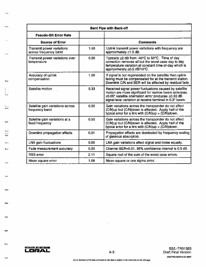
• =
Bent Pipe with Back-off
Pseudo-Bit Error Rate
Source of Error
Transmit power variations 1.50across frequency band
Transmit power variations over 0.50temperature
Accuracy of uplink 1.00compensation
Satellite motion 0.33
Satellite gain variations acrossfrequency band
0.50
0.50Satellite gain variations at afixed frequency
Downlink propagation effects 0.31
LNA gain fluctuations 0.00
Comments
Uplink transmit power variations with frequency areapproximately _+1.5dB.
Typically _+_2dB from -40°C to 50_C. Time of daycorrection removes all but the worst case day to daytemperature variation at constant time-of-day which isapproximately _+0.5dB/10°C.
If signal is not regenerated on the satellite then uplinkfading must be compensated for at the transmit station.Downlink C/N and BER will be affected by residual fade.
Received signal power fluctuations caused by satellitemotion are more significant for narrow beam antennas.•+0.05° satellite orientation error produces _-4-0.33dBsignal level variation at receive terminal in 0.3 ° beam.
Gain variations across the transponder do not affect(C/N)up but (C/N)down is affected. Apply half of thetypical error for a link with (C/N)up = (C/N)down.
Gain variations across the transponder do not affect(C/N)up but (C/N)down is affected. Apply half of thetypical error for a link with (C/N)up = (C/N)down.
Propagation effects are dominated by frequency scalingof gaseous absorption.
LNA gain variations affect signal and noise equally.
Fade measurement accuracy 0.50 Channel BER=0.01,95% confidence interval is 0.5 dB.
RSS error 2.11 Square root of the sum of the worst case errors.
Mean square error 1.06 Mean square or one sigma error.
N_
A-3
Use or disdosu_ of tht _,, _tained on this sheet is subject to the rtst_ti_ on tl_ title p=ge.
SS/L-TR01363Draft Final Version
45 M/'I"R01363/Pa rt3/- 9FJ97
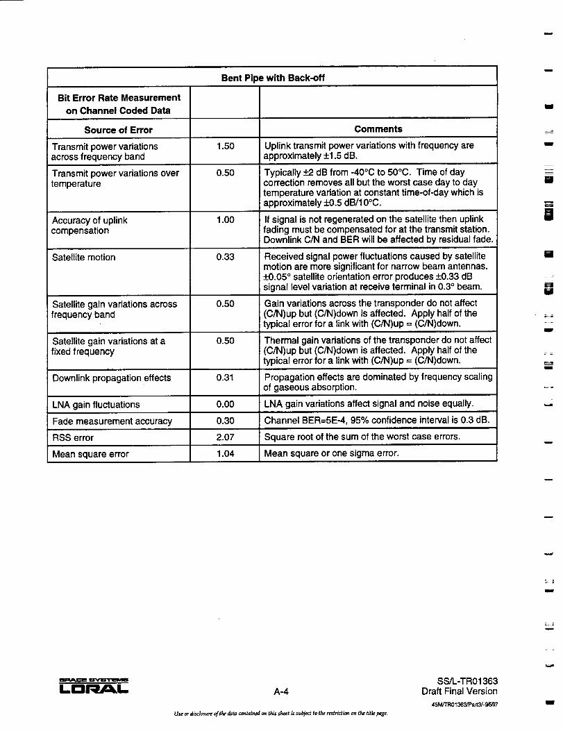
Bent Pipe with Back-off
Bit Error Rate Measurement
on Channel Coded Data
Source of Error Comments
Transmit power variations 1.50 Uplink transmit power variations with frequency areacross frequency band approximately +1.5 dB.
Transmit power variations over 0.50 Typically +_2dB from -40°C to 50°C. Time of daytemperature correction removes all but the worst case day to day
temperature variation at constant time-of-day which isapproximately _+0.5dB/10°C.
Accuracy of uplink 1.00 If signal is not regenerated on the satellite then uplinkcompensation fading must be compensated for at the transmit station.
Downlink C/N and BER will be affected by residual fade.
Satellite motion 0.33 Received signal power fluctuations caused by satellitemotion are more significant for narrow beam antennas._+0.05° satellite orientation error produces _+0,33dBsignal level variation at receive terminal in 0.3 ° beam.
Satellite gain variations across 0.50 Gain variations across the transponder do not affectfrequency band (C/N)up but (C/N)down is affected. Apply half of the
typical error for a link with (C/N)up = (C/N)down.
Satellite gain variations at a 0.50 Thermal gain variations of the transponder do not affectfixed frequency (C/N)up but (C/N)down is affected. Apply half of the
typical error for a link with (C/N)up = (C/N)down.
Downlink propagation effects 0.31 Propagation effects are dominated by frequency scalingof gaseous absorption.
LNA gain fluctuations 0.00 LNA gain variations affect signal and noise equally.
Fade measurement accuracy 0.30 Channel BER=5E-4, 95% confidence interval is 0.3 dB.
RSS error 2.07 Square root of the sum of the worst case errors.
Mean square error 1.04 Mean square or one sigma error., i,.
i
I
iI
=a
lMI
J
Ial
I
UI
L_
w
_Iw
LD L A-4
Useor discbsure of thedata containedonthis sheet is subject to the restrictionon the title page.
SS/L-TR01363Draft Final Version
45M/TR01363/Par13/-9Fu,97
= =
J

Bent Pipe with Back-off
Bit Error Rate Measurementfrom Known Data Pattern
Source of Error
Transmit power variationsacross frequency band
Transmit power variations overtemperatu re
Comments
1.50 Uplink transmit power variations with frequency areapproximately _+1.5dB.
Accuracy of uplinkcompensation
0.50
Satellite motion
Satellite gain variations acrossfrequency band
Satellite gain variations at afixed frequency
Downlink propagation effects
LNA gain fluctuations
Fade measurement accuracy
Total Error
Mean square error
1.00
0.33
0.50
Typically -+2 dB from -40°C to 50°C. Time of daycorrection removes all but the worst case day to daytemperature variation at constant time-of-day which isapproximately _-+0.5dB/10°C.
If signal is not regenerated on the satellite then uplinkfading must be compensated for at the transmit station.Downlink C/N and BER will be affected by residual fade.
Received signal power fluctuations caused by satellitemotion are more significant for narrow beam antennas.-+0.05° satellite orientation error produces __+0.33dBsignal level variation at receive terminal in 0.3 ° beam.
Gain variations across the transponder do not affect(C/N)up but (C/N)down is affected. Apply half of thetypical error for a link with (C/N)up = (C/N)down.
0.50 Gain variations across the transponder do not affect(C/N)up but (C/N)down is affected. Apply half of thetypical error for a link with (C/N)up = (C/N)down.
0.31 Propagation effects are dominated by frequency scalingof gaseous absorption.
0.00 LNA gain variations affect signal and noise equally.
0.50 Channel BER=0.01, 95% confidence interval is _+0.5dB.
2.11 Square root of the sum of the worst case errors.
1.06 Mean square or one sigma error.
:i
A-5
test or disclosurt o_ tht _ta cont_,_ on this skttt is s._tct to tht fish'S:lion _ t_ tit_. _,_.
SS/L-TR01363Draft Final Version
45M/TR01363/Part3/- $F_,_7

Signal to Noise RatioMeasurement
Source of Error
Transmit power variations 1.50across frequency band
0.50Transmit power variations overtemperature
Accuracy of uplinkcompensation
Satellite motion
Satellite gain variations acrossfrequency band
Satellite gain variations at afixed frequency
Downlink propagation effects
1.00
0.33
0.50
0.50
0.31
LNA gain fluctuations 0.00
Fade measurement accuracy 0.10
RSS error 2.05
Mean square error 1.03
Bent Pipe with Back-off
Comments
Uplink transmit power variations with frequency areapproximately _+1.5dB.
Typically +_2dB from -40°C to 50°0. Time of daycorrection removes all but the worst case day to daytemperature variation at constant time-of-day which isapproximately _--K).5dB/10°C.
If signal is not regenerated on the satellite then uplinkfading must be compensated for at the transmit station.Downlink C/N and BER will be affected by residual fade.
Received signal power fluctuations caused by satellitemotion are more significant for narrow beam antennas._+0.05° satellite orientation error produces _+0.33dBsignal level variation at receive terminal in 0.3 ° beam.
Gain variations across the transponder do not affect(C/N)up but (C/N)down is affected. Apply half of thetypical error for a link with (C/N)up = (C/N)down.
Thermal gain variations of the transponder do not affect(C/N)up but (C/N)down is affected. Apply half of thetypical error for a link with (C/N)up = (C/N)down.
Propagation effects are dominated by frequency scalingof gaseous absorption.
LNA gain variations affect signal and noise equally.
For Eb/No > 5 dB, 95% confidence interval is 0.1 dB.
Square root of the sum of the worst case errors.
Mean square or one sigma error.
m
J
i
H.=,.m
m
mm
==
b
.lk.=
lmm,aJ_! _
LD I.. A-6
Use or disclosure of the data contained on this sheet is subject to the restriction on the title yage.
SS/L-TR01363Draft Final Version
45M/'I'R01363/Pad3/-gFj97

Bent Pipe with Saturated Transponder
Low Cost Beacon Receiver
Residual
Source of Error Error, [_+dB] Comments
0.31Beacon power fluctuations atreceive terminal
Receive antenna pointing errors 0.90and efficiency variations
Receive gain fluctuations 1.00
Beacon power levelmeasurement accuracy
RSS Error
0.75
Degradation estimate accuracy
1.57
Mean square error 0.79
_+1.25dB
Fade estimate errors caused by satellite beacon powerand pointing errors are much less than propagationeffects. Propagation effects are dominated byfrequency scaling of gaseous absorption.
Dominated by inaccurate frequency scaling of feedwindow wetting.
Residual error will be related to the worst case day-to-day temperature change at a constant time of day.
Expensive beacon receivers can provide _-+0.25dBaccuracy. Accuracy of low cost receiver is estimated tobe _+0.75dB., i ,
Worst case values above are interpreted as two sigmavalues. Error is less than value 95% of time.
Beacon receiver measures fading on path whilecomparison is performed on accuracy of degradationestimate. Terminal must assume system and sky noisetemperature and calculate degradation from fademeasurement.
m_
LDl b¢ l,. A-7
Use or disclosure of the data contained an this sh_t is subject to the restriction on the title page.
SS/L-TR01363Draft Final Version
45MfT'R01363/Patt3/-gra_7

Bent Pipe with Saturated Transponder
Automatic Gain Control SignalMeasurement
Residual
Source of Error Error, [_+dB] Comments
Transmit power variations 0.15 Uplink transmit power variations with frequency ofacross frequency band _+1.5dB will be reduced to approximately _-K).15dB in
saturated transponder.
Transmit power variations over 0.05 Uplink transmit power variations with temperature oftemperature _+0.5dB will be reduced to approximately _-K).05dB in
saturated transponder.
Accuracy of uplink 0.10 Uplink compensation errors of _+1.0dB will be reducedcompensation to approximately _.1 dB in saturated transponder.
.. n.
Satellite motion 0.33 Received signal power fluctuations caused by satellitemotion are more significant for narrow beam antennas._+0.05° satellite orientation error produces _--*-0.33dBsignal level variation at receive terminal in 0.3 ° beam.
Satellite gain variations across 0.50 Gain variations across the transponder do not affectfrequency band (C/N)up but (C/N)down is affected. Apply half of the
typical error for a link with (C/N)up = (C/N)down.
Satellite gain variations at a 0.50 Thermal gain variations of the transponder do not affectfixed frequency (C/N)up but (C/N)down is affected. Apply half of the
typical error for a link with (C/N)up = (C/N)down.
Downlink propagation effects 0.31 Propagation effects are dominated by frequency scalingof gaseous absorption.
LNA gain fluctuations 1.00 LNA gain variations affect signal and noise equally.
RSS of worst case errors 1.32 Error is less than this value 95% of the time.,,in i,l.,.
RSS error 0.66 RMS error or one sigma error.
Mean square error in fade 0.95 [Eb/No] clear-sky =9 dBestimate
Mean square error in 2.17 Fade =5-+1.5 dB, Tin=280 -+10, Ts=230-+10degradation estimate
u
Im
t
u
m
!il
m
w
_ 15"Yu"rl_l_lS
A-8
Use or disclosure _f the data contained on this shert is subject to the restriction on the title page.
SS/L-TR01363Draft Final Version
45M/TRo 1363/Part3/-_-_J7

Bent Pipe with Saturated Transponder
Pseudo-Bit Error Rate
Source of Error Comments
Transmit power variations 0.15 Uplink transmit power variations with frequency ofacross frequency band +1.5 dB will be reduced to approximately :L-0.15dB in
saturated transponder.
Transmit power variations over 0.05 Uplink transmit power variations with temperature oftemperature _+0.5dB will be reduced to approximately _+0.05dB in
saturated transponder.
Accuracy of uplink 0.10 Uplink compensation errors of _+1.0dB will be reducedcompensation to approximately _-_+0.1dB in saturated transponder.
Satellite motion 0.33 Received signal power fluctuations caused by satellitemotion are more significant for narrow beam antennas._+0.05° satellite orientation error produces _+0.33dBsignal level variation at receive terminal in 0.3 ° beam.
Satellite gain variations across 0.50 Gain variations across the transponder do not affectfrequency band (C/N)up but (C/N)down is affected. Apply half of the
typical error for a link with (C/N)up = (C/N)down.
Satellite gain variations at a 0.50 Gain variations across the transponder do not affectfixed frequency (C/N)up but (C/N)down is affected. Apply half of the
typical error for a link with (C/N)up = (C/N)down.
Downlink propagation effects 0.31 Propagation effects are dominated by frequency scalingof gaseous absorption.
LNA gain fluctuations " 0.00 LNA gain variations affect signal and noise equally.
Fade measurement accuracy 0.50 Channel BER=O.01,95% confidence interval is 0.3 dB.
RSS error 0.99 Square root of the sum of the worst case errors.
Mean square error 0.50 Mean square or one sigma error.
r •
N g'V_a'rlm_qEi
LI:31" B£ I.. L A--9
Use or disclosure of the daLa c_ntained on this sh_ is subject to the restrlction on the title paSe.
SS/L-TR01363Draft Final Version
45M/TR01363/Patt3/-_J97

Bent Pipe with Saturated Transponder
Bit Error Rate Measurement
on Channel Coded Data
Source of Error Comments
Transmit power variations 0.15 Uplink transmit power variations with frequency ofacross frequency band _+1.5dB will be reduced to approximately _+0.15dB in
saturated transponder.
Transmit power variations over 0.05 Uplink transmit power variations with temperature oftemperature _+0.5dB will be reduced to approximately _+0.05dB in
saturated transponder.
Accuracy of uplink 0.10 Uplink compensation errors of _+1.0dB will be reducedcompensation to approximately _+0.1dB in saturated transponder.
Satellite motion 0.33 Received signal power fluctuations caused by satellitemotion are more significant for narrow beam antennas._-_-+0.05° satellite orientation error produces -+0.33 dBsignal level variation at receive terminal in 0.3 ° beam.
Satellite gain variations across 0.50 Gain variations across the transponder do not affectfrequency band (C/N)up but (C/N)down is affected. Apply half of the
typical error for a link with (C/N)up = (C/N)down.
Satellite gain variations at a 0.50 Gain variations across the transponder do not affectfixed frequency (C/N)up but (C/N)down is affected. Apply half of the
typical error for a link with (C/N)up = (C/N)down.
Downlink propagation effects 0.31 Propagation effects are dominated by frequency scalingof gaseous absorption.
LNA gain fluctuations 0.00 LNA gain variations affect signal and noise equally.
Fade measurement accuracy 0.30 Channel BER=5E-4, 95% confidence interval is 0.3 dB.
RSS error 0.91 Square root of the sum of the worst case errors.,, m
Mean square error 0.46 Mean square or one sigma error.
m
m
BIB
IBIB
m
U
I
: c
w
A-10
Useordisclosure o/the _,, c_tained on this sheetis subject to therestriction on tile title pa_e.
SS/L-TR01363Draft Final Version
45M/TR013_art3/-9_g7 I

Bent Pipe with Saturated Transponder
Bit Error Rate Measurement
from Known Data Pattern
Source of Error Comments
Transmit power variations 0.15 Uplink transmit power variations with frequency ofacross frequency band +1.5 dB will be reduced to approximately _+0.15dB in
saturated transponder.
Transmit power variations over 0.05 Uplink transmit power variations with temperature oftemperature _+0.5dB will be reduced to approximately _-_+0.05dB in
i saturated transponder.
Accuracy of uplink 0.10 Uplink compensation errors of +_1.0dB will be reducedcompensation to approximately _-+0.1dB in saturated transponder.
Satellite motion 0.33 Received signal power fluctuations caused by satellitemotion are more significant for narrow beam antennas.+-0.05° satellite orientation error produces _-*-0.33dBsignal level variation at receive terminal in0.3 ° beam.
Satellite gain variations across 0.50 Gain variations across the transponder do not affectfrequency band (C/N)up but (C/N)down is affected. Apply half of the
typical error for a link with (C/N)up -- (C/N)down.
Satellite gain variations at a 0.50 Gain variations across the transponder do not affectfixed frequency (C/N)up but (C/N)down is affected. Apply half of the
typical error for a link with (C/N)up = (C/N)down.
Downlink propagation effects 0.31 Propagation effects are dominated by frequency scalingof gaseous absorption.
LNA gain fluctuations 0.00 LNA gain variations'affect signal and noise equally.
Fade measurement accuracy 0.50 Channel BER=0.01, 95% confidence interval is +-0.5 dB.
Total Error 0.99 Square root of the sum of the worst case errors.
Mean square error 0.50 Mean square or one sigma error.
"_=....
r__
L_L
w
m
w
m
I.DI= .I L A-11
Use or disclosure _f tl_ ,_ta con_aln_ _'Itl_ sheet issu_ect to _he testricfionon _he riflepage.
SS/L-TR01363Draft Final Version
45M/TR01363,_Pa rt 3/- 9r--_97
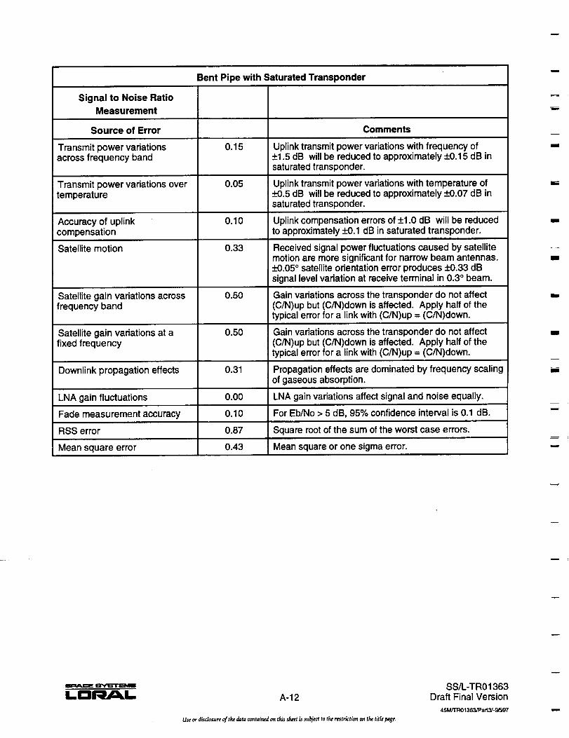
Bent Pipe with Saturated Transponder
Signal to Noise RatioMeasurement
Source of Error Comments
Transmit power variations 0.15 Uplink transmit power variations with frequency ofacross frequency band +_1.5dB will be reduced to approximately +-0,15 dB in
saturated transponder.i n i= n ill
Transmit power variations over 0.05 Uplink transmit power variations with temperature oftemperature __+0.5dB will be reduced to approximately _-K),07dB in
saturated transponder.
Accuracy of uplink 0,10 Uplink compensation errors of +_1.0dB will be reducedcompensation to approximately _-+O.1dB in saturated transponder.
Satellite motion 0.33 Received signal power fluctuations caused by satellitemotion are more significant for narrow beam antennas._-+0.05° satellite orientation error produces _-+0.33dBsignal level variation at receive terminal in 0.3 ° beam.
Satellite gain variations across 0.50 Gain variations across the transponder do not affectfrequency band (C/N)up but (C/N)down is affected. Apply half of the
typical error for a link with (C/N)up = (C/N)down.
Satellite gain variations at a 0.50 Gain variations across the transponder do not affectfixed frequency (C/N)up but (C/N)down is affected. Apply half of the
typical error for a link with (C/N)up = (C/N)down.
Downlink propagation effects 0.31 Propagation effects are dominated by frequency scalingof gaseous absorption.
LNA gain fluctuations 0.00 LNA gain variations affect signal and noise equally.
Fade measurement accuracy 0.10 For Eb/No > 5 dB, 95% confidence interval is 0.1 dB.
RSS error 0.87 Square root of the sum of the worst case errors.
Mean square error 0.43 Mean square or one sigma error.
m
I
.=
U
U
i
U
Nm
w
m
m
_ Q'Ytn"l_lm
LDREJC L A-12
Use ordisclosureoft_ _ta conralnedon thisskeetissubjecttotherestri_ti_on thetizlepa_.
SS/L-TR01363Draft Final Version
45M/TR01363/Part 3/-gFoB7

w
w
On-board Processing
Low Cost Beacon Receiver
Residual
Source of Error Error, [_+dB] Comments
Beacon power fluctuations at 0.31 Fade estimate errors caused by satellite beacon powerreceive terminal and pointing errors are much less than propagation
effects. Propagation effects are dominated byfrequency scaling of gaseous absorption.
Receive antenna pointing errors 0.90 Dominated by inaccurate frequency scaling of feedand efficiency variations window wetting.
Receive gain fluctuations 1.00 Residual error will be related to the worst case day-to-day temperature change at a constant time of day.
Beacon power level 0.75 Expensive beacon receivers can provide _-+0.25dBmeasurement accuracy accuracy. Accuracy of low cost receiver is estimated to
be -+0.75 dB.
RSS Error 1.57 Worst case values above are interpreted as two sigmavalues. Error is less than value 95% of time.
Mean square error 0.79
Degradation estimate accuracy _+1.25dB Beacon receiver measures fading on path whilecomparison is performed on accuracy of degradationestimate. Terminal must assume system and sky noisetemperature and calculate degradation from fademeasurement.
w
m
L__
w
A-13
Use or disclosure of the data contained on this sheet is su_ect to the restrictio_ on the title page.
SS/L-TR01363Draft Final Version
45 M/TR01363/Pa rt3/- 9,5_'/
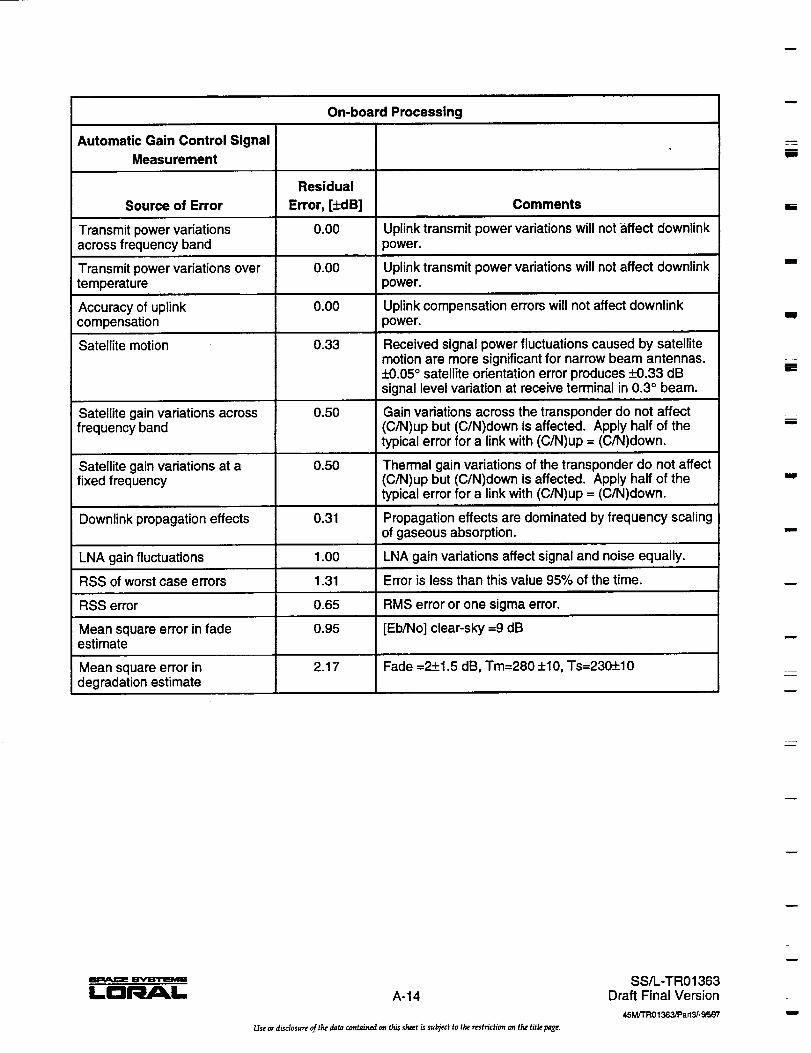
On-board Processing
Automatic Gain Control SignalMeasurement
Residual
Source of Error Error, [_+dB] Comments
0.00Transmit power variationsacross frequency band
Transmit power variations overtemperature
0.00
Uplink transmit power variations will not affect downlinkpower.
Uplink transmit power variations will not affect downlinkpower.
Accuracy of uplink 0.00 Uplink compensation errors will not affect downlinkcompensation power.
Satellite motion 0.33 Received signal power fluctuations caused by satellitemotion are more significant for narrow beam antennas._+0.05° satellite orientation error produces _-H3.33dBsignal level variation at receive terminal in 0.3 ° beam.
Satellite gain variations across 0.50 Gain variations across the transponder do not affectfrequency band (C/N)up but (C/N)down is affected. Apply half of the
typical error for a link with (C/N)up = (C/N)down.
Satellite gain variations at a 0.50 Thermal gain variations of the transponder do not affectfixed frequency (C/N)up but (C/N)down is affected. Apply half of the
typical error for a link with (C/N)up = (C/N)down.
Downlink propagation effects 0.31 Propagation effects are dominated by frequency scalingof gaseous absorption.
LNA gain fluctuations 1.00 LNA gain variations affect signal and noise equally.
RSS of worst case errors 1.31 Error is less than this value 95% of the time.
RSS error 0.65 RMS error or one sigma error.
Mean square error in fade 0.95 [Eb/No] clear-sky =9 dBestimate
Mean square error in 2.17 Fade =?__.1.5dB, Tm=280 __.10,Ts=230!-_10degradation estimate
m
m
m
U
m
m
U
LIl31 =C L A-14
Use or disclosure of the data contained on this sheet is subject to the restriction on th_ title page.
SS/L-TR01363Draft Final Version
45 M/TRO 1363/Pa rt3/'-_Vg"/

w
w
On-board Processing
Pseudo-Bit Error Rate
Source of Error Comments
Transmit power variations 0.15 Uplink transmit power variations with frequency ofacross frequency band _+1.5dB will be reduced to approximately _+0.15dB in
saturated transponder.
Transmit power variations over 0.05 Uplink transmit power variations with temperature oftemperature _+0.5dB will be reduced to approximately _+0.05dB in
saturated transponder.
Accuracy of uplink 0.10 Uplink compensation errors of _+1.0dB will be reducedcompensation to approximately _+0.1dB in saturated transponder.
Satellite motion 0.33 Received signal power fluctuations caused by satellitemotion are more significant for narrow beam antennas._--H).05° satellite orientation error produces _-+0.33dBsignal level variation at receive terminal in 0.30 beam.
Satellite gain variations across 0.50 Gain variations across the transponder do not affectfrequency band (C/N)up but (C/N)down is affected. Apply half of the
typical error for a link with (C/N)up = (C/N)down.
Satellite gain variations at a 0.50 Gain variations across the transponder do not affectfixed frequency (C/N)up but (C/N)down is affected. Apply half of the
typical error for a link with (C/N)up -- (C/N)down.
Downlink propagation effects 0.31 Propagation effects are dominated by frequency scalingof gaseous absorption.
LNA gain fluctuations 0.00 LNA gain variations affect signal and noise equally.
Fade measurement accuracy 0.50 Channel BER=0.01, 95% confidence interval is 0.3 dB.
RSS error 0.99 Square root of the sum of the worst case errors.
Mean square error 0.50 Mean square or one sigma error.
w
-.==_
w
w
m_
LC:IIRM L A-15
Use or disclosure of the data contained on this sheet is su_ect to the restriction on the title page.
SS/L-TR01363Draft Final Version
45 M/I'_ 01363JPa rt 3/- _'/

On-board Processing
Bit Error Rate Measurement
on Channel Coded Data
Source of Error Comments
Transmit power variations 0.00 Uplink transmit power variations will not affect downlinkacross frequency band power.
Transmit power variations over 0.00 Uplink transmit power variations will not affect downlinktemperature power.
Accuracy of uplink 0.00 Uplink compensation errors will not affect downlinkcompensation power.
Satellite motion 0.33 Received signal power fluctuations caused by satellitemotion are more significant for narrow beam antennas._+0.05° satellite orientation error produces _--H).33dBsignal level variation at receive terminal in 0.3 ° beam.
Satellite gain variations across 0.50 Gain variations across the transponder do not affectfrequency band (C/N)up but (C/N)down is affected. Apply half of the
typical error for a link with (C/N)up = (C/N)down.
Satellite gain variations at a 0.50 Gain variations across the transponder do not affectfixed frequency (C/N)up but (C/N)down is affected. Apply half of the
typical error for a link with (C/N)up = (C/N)down.
Downlink propagation effects 0.31 Propagation effects are dominated by frequency scalingof gaseous absorption.
LNA gain fluctuations 0.00 LNA gain variations affect signal and noise equally.
Fade measurement accuracy 0.30 Channel BER=5E-4, 95% confidence interval is 0.3 dB.
RSS error 0.89 Square root of the sum of the worst case errors.
Mean square error 0.45 Mean square or one sigma error.
ii
ill
Ill
il
lira
im
llll
U
N_
A-16
Use or disclosure _ the data contained on this sheet is subject to the restriction on the title page.
SS/L-TR01363Draft Final Version
45 M/'fR01363/P a rt3/- 9r.J97

w
w
=
On-board Processing
Bit Error Rate Measurementfrom Known Data Pattern
Source of Error
Transmit power variations 0.00across frequency band
Transmit power variations over 0.00temperature
0.00Accuracy of uplinkcompensation
Satellite motion 0.33
Satellite gain variations across 0.50frequency band
Satellite gain variations at a 0.50fixed frequency
Downlink propagation effects 0.31
LNA gain fluctuations 0.00
Fade measurement accuracy 0.50
Total Error 0.98
Mean square error 0.49
Comments
Uplink transmit power variations will not affect downlinkpower.
Uplink transmit power variations will not affect downlinkpower.
Uplink compensation errors will not affect downlinkpower.
Received signal power fluctuations caused by satellitemotion are more significant for narrow beam antennas._+0.05° satellite orientation error produces _-_+0.33dBsignal level variation at receive terminal in 0.3 ° beam.
Gain variations across the transponder do not affect(C/N)up but (C/N)down is affected. Apply half of thetypical error for a link with (C/N)up = (C/N)down.
Gain variations across the transponder do not affect(C/N)up but (C/N)down is affected. Apply half of thetypical error for a link with (C/N)up = (C/N)down.
Propagation effects are dominated by frequency scalingof gaseous absorption.
1.,
LNA gain variations affect signal and noise equally.
Channel BER=0.01,95% confidence interval is _+0.5dB.
Square root of the sum of the worst case errors.
Mean square or one sigma error.
m_
I-1:31=J./ L A-17
Useor disclosure of thedata c_ntainedon this sheetis subject to the restrictionon the title page.
SS/L-TR01363Draft Final Version
45M,'TRO1363/Part3/-9FJ97

On-board Processing
Signal to Noise RatioMeasurement
Source of Error
Transmit power variationsacross frequency band
Transmit power variations overtemperature
Accuracy of uplinkcompensation
Satellite motion
Satellite gain variations acrossfrequency band
Satellite gain variations at afixed frequency
Downlink propagation effects
LNA gain fluctuations
Fade measurement accuracy
RSS error
Mean square error
0.00
0.00
0.00
0.33
0.50
0.50
0.31
0.00
0.10
0.85
0.42
Comments
Uplink transmit power variations will not affect downlinkpower.
Uplink transmit power variations will not affect downlinkpower.
Uplink compensation errors will not affect downlinkpower.
Received signal power fluctuations caused by satellitemotion are more significant for narrow beam antennas._--H).05° satellite orientation error produces _--K).33dBsignal level variation at receive terminal in 0.3 ° beam.
Gain variations across the transponder do not affect(C/N)up but (C/N)down is affected.
Gain variations across the transponder do not affect(C/N)up but (C/N)down is affected. Apply half of thetypical error for a link with (C/N)up = (C/N)down.
Propagation effects are dominated by frequency scalingof gaseous absorption. Apply half of the typical error fora link with (C/N)up = (C/N)down.
LNA gain variations affect signal and noise equally.
For Eb/No > 5 dB, 95% confidence interval is 0.1 dB.
Square root of the sum of the worst case errors.
Mean square or one sigma error.
iil
m
m
I
Ill
m
II
I
m
Ill
m
m
i
_ B'Y'B'IrlmMa
LD L A-18
Use or disclosure of the data contained on this sheet is subject to the restriction on the title page.
SS/L-TR01363Draft Final Version
45M/r'R01363/Part3/- 9Fu/97 I

APPENDIX B -- HEXAGONAL ARRAY NUMEROLOGY AND ACTIVEAREA FOR CIRCULAR ELEMENTS
w
L
Hexagonal array numerology is presented followed by calculation of the active area of a
hexagonal array of circular feed horns. It is determined that the ratio of active area to total
area is about 0.91 for large arrays.
In a hexagonal array the total numbers of elements, n_n_,for regular hexagonal fill areas are 7,
19, 37, 61, 91, 127, etc. The number of elements on a principal diagonal of the hexagonal
area can be defined as:
number of elements on principal diagonal = 2k+1
where k=l for n=7, k=2 for n=19, k=3 for n=37, etc.
expressed as a function of k as:
n = 6(1+(k-1)/2)k + 1
With this nomenclature, n may be
Let the hexagonal fill area be inscribed within the smallest circle such that no part of the
hexagonal area is outside of the circle. The diameter of this circle is equal to (2k+1) D h,
where D h is the diameter of an individual feed horn.
The active area of the feed array is equal to the area of all of then [= 6(1+(k-1)/2)k + 1] feed
horn apertures, or nA h, where A h = _(Dh/2) 2 is the area of a single feed horn aperture. The
total area of the feed array is the active area plus the area taken by all of the interstitial
areas between the feed horns. Each such interstitial area, Ai, is obtained as follows:
a i = (area of an equilateral triangle with vertices at the centers of three adjacent
feed horns) - 3 (one-sixth the area of a single feed horn aperture)
(1/2) D h D h cos(30 °) - (3/6)_(Dh/2) 2
0.16125 (Dh/2) 2 = 0.0513275_ (Dh/2) 2
It is easy to count the number of interstitial areas, i_,for each hexagonal array and establish
a functional relationship with k. The result of this effort is:
i = 6k 2
= =
r_
B-1
Use or disclosure of the data contained on this sheet is subject to the restriction on the title page.
SS/L-TR01363Draft Final Version
45 M/I"R01363/Pa rt3/- _-J97

The ratio Ra/t of active area to total area of a hexagonal array is then given by:
Ra/t = (active area) / [(active area) + (interstitial area)]
= nAh/[nA h + 6k2Ai]
= n_(Dh/2)2/[n_(Dh/2) 2 + 6k 2 0.0513275 _(Dh/2) 2]
= [6(l+(k-1)/2)k + 1]/[6(1+(k-1)/2)k + 1 + 6k 2 (0.0513275)]
= [3k 2 + 3k + 1]/[3.308k 2 + 3k + 1]
Values for Ra/t are given in Table B-1.
To obtain an array with 1323 active elements, the value of k should be about 21. Therefore,
the diameter of the array is 43 feed horns. For any given feed-horn spacing, in
wavelengths, the diameter may be calculated.
For example, if horn spacing is 2.6 wavelengths at 19.2 GHz, the array diameter is given by:
array diameter = 43 x 2.6 (11.785/19.2) inches
= 68.6 inches
U
b.--
g
m
I
I
[]m
m
u
LD_L B-2
Use or disclosure of the data contained on this sheet is subject to the restriction on the title page.
SS/L-TR01363Draft Final Version
45M/'FR01363/Part 3/- _-,J37

w Table B-1. Table of Values of ILa/t for k=1,2, ..., 6
n
1
2
3
4
5
6
7m
8
(number of feeds in
regular hexagonal grid
array)
611+(k-1)/2]k+1
0 1
7
9
10
11
12
13
14
15
16
17
18
19
20
21
22
23
24
25
19
37
61
91
127
169
217
271
331
397
469
547
631
(number of interstices
within regular
hexagonal grid array)
6k2
919
1027
1141
1261
1387
1519
1657
1801
1951
Ra_ = [3k 2 + 3k + 1]/[3.308k 2 + 3k + 1]
Ra/t
(ratio of active area
to total area of
array)*
0 1
6 0.9579
24 0.9391
54 0.9303
96 0.9253
150 0.9220
216 0.9197
282 0.9180
384 0.9167
486 0.9157
600 0.9149
726 0.9142
864 0.9136
1014 0.9131
1176 0.9127
721 1350 0.9123
817 1536 0.9120
1734 0.9117
1944 0.9114
2166 0.9112
2400 0.9110
2646 0.9108
2904 0.9106
3174 0.9105
3456 0.9103
3750 0.9102
w
B-3
Use or disclosure of the data contained on this sheet is subject to the restriction on the title page.
SS/L-TR01363Draft Final Version
45MfTR01363JPart3/- 9F_7

=,.,=.
in
I
i
i
If
i

I i
I I
II •
w
w
qjuf
LF_
U
E_L_
U
w

w
z
im
ml
mE
LrIF_IR
r
W
m
lil
h_
[]
II
_mI
m
mm
M
m
m
i
m
I
II
mI
I

r
= ,
• Jz
I7
=
U
w
== =
L.
REPORT DOCUMENTATION PAGE FormApprovedOMB No. 0704-0188
Public reporting burden for this collection of information is Ostimeted to average 1 hour per response, inclu_ng the time for reviewing instructions, searching existing data sources,
,ecl._p..oT w_ormai_)=_c=u_ng sugpst_n=s _r r_uc_g m,s Duro__, zo wa.snlngton Heaoquartars :sen/cos, utrectorate for In fi_tetlorl Operations and Reports, 1215 Jeffersonaws r.gnway, butte 12o4, /_l=ngton,v_ ZZZtZZ'43orx,and tO me unee o=Management and Budget.Paperwork ReductionProject (0704-0188), Washington. DC 20503.
1. AGENCY USE ONLY (Leave blank) 2. HEPORT DATE 3. REPORT TYPE AND DATES COVERED
December 1997 Final Coal]actor Report4. roLE ANDSUB'ffr'L/_
Rain Fade Compensation for Ka-Band Communications Satellites
6. AUTHOR(S)
W. Carl Mitchell, Lan Nguyen, Asoka Dissanayake, and Brian Markey
7. PERFORMING ORGANIZATION NAME(S) AND ADDRESS(ES)
Space Systems/LORAL3825 Fabian WayPalo Alto, California 94303--4604
9. SPONSORING/MONIT()RING _.GENCY NAME(S) AND ADDRESS(ES)
National Aeronautics and Space AdministrationLewis Research Center
Cleveland, Ohio 44135-3191
S. FUNDING NUMBERS
WU-315-90-2CNAS3-27559
8. PERFORMING ORGANIZATIONREPORT NUMBER
E-11024
10. SPONSORING/MONITORINGAGENCY REPORT NUMBER
NASACR_97-206591SS/LTR01363
11. SUPPLEMENTARY NOTES
W. Carl Mitchell, Space Systems/Loral, 3825 Fabian Way, Palo Alto, California 94303-4606; Lan Nguyen, AsokaDissanayake, and Brian Markey, COMSAT Laboratories, Clarksburg, Maryland. Project Manager, Clifford H. Arth, SpaceCommunications Office, NASA Lewis Research Center, organization code, (216) 433-3460.
12a. DISTRIBUTION/AVAILABILITY STATEMENT 12b. DISTRIBUTION CODE
Unclassified - Unlimited
Subject Category: 17 Distribution: Nonstandard
This publication is available from the NASA Center for AeroSpace Information, (301) 621-0390.1
13. ABSTRACT (Mexlmum 200 words)
This report provides a review and evaluation of rain fade measurement and compensation techniques for Ka-band satellitesystems. This report includes a description of and cost estimates for performing three rain fade measurement and compen-sation experiments. The first experiment deals with rain fade measurement techniques while the second one covers therain fade compensation techniques. The third experiment addresses a feedback flow control technique for the ABR service(for ATM-based traffic). The following conclusions were observed in this report; a sufficient system signal margin shouldbe allocated for all carriers in a network, that is a fixed clear-sky margin should be typically in the range of 4-5 dB andshould be more like 15 dB in the up link for moderate and heavy rain zones; to obtain a higher system margin it isdesirable to combine the uplink power control technique with the technique that implements the source information rateand FEC code rate changes resulting in a 4-5 dB increase in the dynamic part of the system margin. The experiments
would assess the feasibility of the fade measurements and compensation techniques, and ABR feedback control technique.
14. SUBJECT TERMS
ACTS; Rain fade;Ka-band; Satellites
17. SECU_T'f CLASSIFICATION 18. SECURITY CLASSIFICATION
OF REPORT OF THIS PAGE
Unclassified Unclassified
NSN 7540-01-280-5500
19. SECURITY CLASSIFICATIONOF ABSTRACT
Unclassified
lS. NUMBER OF PAGES
16. PRICE CODE
A0820. MMrrATION OF ABSTRACT
Standard Form 298 (Rev. 2-89)
Prescribed by ANSI Std. Z39-18298-102
I
li
im
_--__
= =
I
I
U
I
....... 4 _I
=
iIlIIm
m
I
I
I


