Railways and the Raj: The Economic Impact of Transportation Infrastructure Dave Donaldson...
24
Railways and the Raj: The Economic Impact of Transportation Infrastructure Dave Donaldson ([email protected])
-
Upload
baldwin-bailey -
Category
Documents
-
view
218 -
download
2
Transcript of Railways and the Raj: The Economic Impact of Transportation Infrastructure Dave Donaldson...
Railways and the Raj: The Economic Impact of
Transportation Infrastructure
Dave Donaldson

Research Questions
• What is the effect on economic outcomes of opening up to external (ie. international) trade?
• What is the effect on economic outcomes of enabling internal (ie. inter-regional) trade?
• What are the economic gains from improving transportation infrastructure?
• Why economic change underpins these effects?

Motivation
• Our understanding of the effects of openness to trade is still incomplete:– External trade: usually all of country liberalises trade
at same time, so finding counterfactuals is difficult– Internal trade: virtually unexplored, for lack of data
• Transportation infrastructure is a dominant important policy issue in LDCs (eg WDR 1994), yet evidence base is lacking– very hard to evaluate, due to endogenous placement

This paper
• Collect new dataset on prices, wages, production (agricultural), and trade at the district-level (N=~300) in India, from 1870-1925
• Use features of colonial construction of railways (1850-1900) in India as a set of ‘natural experiments’ in openness– Military motive (responding to domestic and foreign aggression)– Famine-prevention motive
• Study impact of railways on agricultural output• Interpret this impact in context of a simple trade model
– Predicts specialisation in comparative advantage crops
• Use data on internal and external trade flows to examine this mechanism
• Where data permits, examine other possible mechanisms (capital and labour reallocations, technological change)
Why Colonial India?
• This region and period of history offer a number of institutional and methodological advantages:– Railway system was dramatic shock (in most of India
at this time, road and river transport was poor/non-existent)
– Railway line placement motives were non-economic in many instances
– Availability of unique internal trade data• Allows external trade to be studied using within-country
variation• Allows internal trade to be studied

Related Literature
• Effect of openness, using natural experiment approach:– Bernhofen-Brown (JPE ‘03, AER ‘04) use Japan’s
1851 (forced) openness to test comparative advantage mechanisms behind opening
– Michaels (2006) uses US Interstate highway expansion to study effect of openness on skill premium
• Quantifying the gains from railways:– Fogel (1967) on USA: uses ‘social savings’ technique,
ignores endogenous placement– Hurd (1998) on India: same method; finds large effect
(9% of GDP in 1900)

This presentation
– Background:• Railways• Economic environment
– Elements of a simple theoretical framework for thinking about these issues
– Data– Empirical method
• Identification strategy for estimating effect of railways
• What economic mechanisms underpin this effect?

Background: Railways
• Principal public investment in colonial India (over half of government spending)
• Mixtures of pure public and public-private provision, but Indian Government always determined route selection
• 95% of current lines built in 1853-1930
• 1870-1920 was highest growth period

1870
65 districts had railway somewhere in district

1900
170 districts had railway somewhere in district

1930
220 districts had railway somewhere in district

Background: Economic Environment (1)
• Structure of economy in 1870:– Agriculture: 68% of GDP, (73% of labour)– Small-scale manuf. and services: 26%, (26%) – Large-scale manufacturing: 0.5%, (0.2%)
• Structure of economy in 1930:– Agriculture: 59%, (75%)– Small-scale manuf. and services: 34%, (23%)– Large-scale manufacturing: 4%, (2%)
Background: Economic Environment (2)
• Effect of railways on transport costs:– Standard estimates suggest that the pure
freight costs of railways were 5-10 times lower than on alternative method (bullock carts)
– However, this ignores other savings:• Bullocks/roads seasonal (bullocks need
food/water, roads unpassable for

Data (1870-1930)• Agricultural production (annual, ~300 districts/native
states):– Yields, by crop (~15 crops)– Land area allocations, by crop– Capital stocks (livestock, carts)– Irrigated areas, by crop
• Prices and wages (annual, ~200 districts/native states)– Prices: by ~30 commodities– Wages: by ~5 occupations (skilled and unskilled)
• Trade (annual, ~70 trade blocks):– Internal trade: full block-to-block matrix of trade flows (but intra-
block diagonals empty)– External trade: trade by port, by foreign country– All in physical units, by commodity (~100 goods), by mode of
transportation (rail, river, coast)

Limitations of the Data
• Agricultural Yields:– Subject of much controversy among econ historians– Created by multiplying normal yields (factual) by subjective
‘conditioning factor’– But largely corroborated by quinquennial crop-cutting surveys
(and no obvious signs that this is not just classical ME)
• Trade data:– External trade flows by block not collected
• have to make assumptions of constant port consumption, and no port transformation
– Roads data very limited in coverage – Lack of unit values may obscure quality-differentiation within
observed commodity classifications
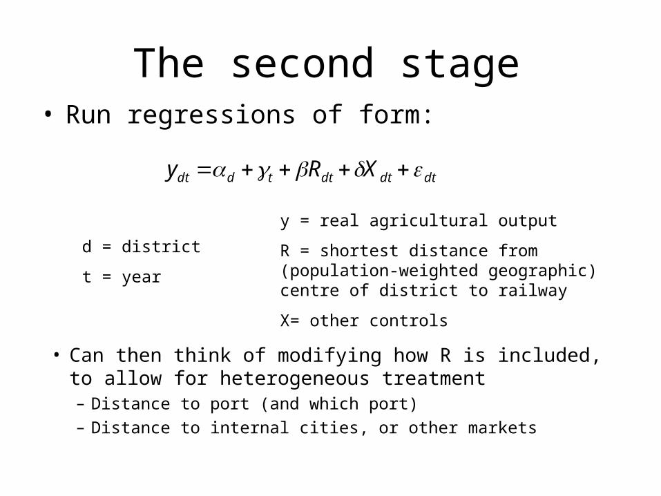
The second stage• Run regressions of form:
dtdtdttddt XRy
y = real agricultural output
R = shortest distance from (population-weighted geographic) centre of district to railway
X= other controls
d = district
t = year
• Can then think of modifying how R is included, to allow for heterogeneous treatment – Distance to port (and which port)
– Distance to internal cities, or other markets

The first stage
dtdtdttddt XZR
•Run regressions of form:
•Where Z is a variable that predicts R, but has no direct effect on y

General IV set-up (1)
• Railways are lines designed to connect two points, A and B
• For any points (A,B), and the observed railway between them, can ask:– What is the effect of the railway on A or B?– What is the effect of the railway on intervening point C?
A
C
B
RAdt ~=0 RBdt ~=0
RCdt = d
d
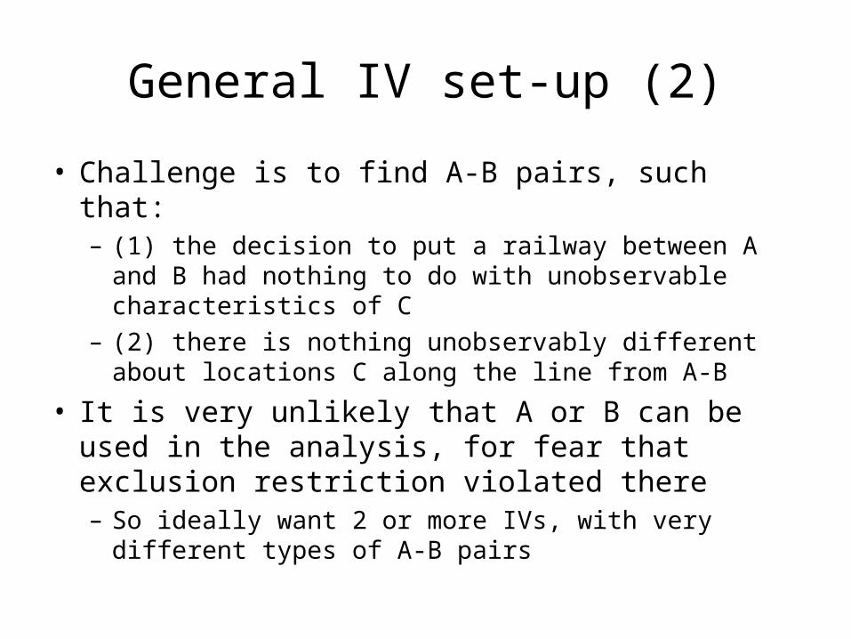
General IV set-up (2)
• Challenge is to find A-B pairs, such that:– (1) the decision to put a railway between A and B had
nothing to do with unobservable characteristics of C– (2) there is nothing unobservably different about
locations C along the line from A-B
• It is very unlikely that A or B can be used in the analysis, for fear that exclusion restriction violated there– So ideally want 2 or more IVs, with very different
types of A-B pairs
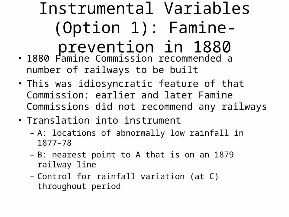
Instrumental Variables (Option 1): Famine-prevention in 1880
• 1880 Famine Commission recommended a number of railways to be built
• This was idiosyncratic feature of that Commission: earlier and later Famine Commissions did not recommend any railways
• Translation into instrument– A: locations of abnormally low rainfall in 1877-78– B: nearest point to A that is on an 1879 railway line – Control for rainfall variation (at C) throughout period

Lines suggested in 1880 Famine
Commission report

Instrumental Variables (Option 2) – Military Transportation
• Macpherson (1955) estimates that over half of track placement decisions were militarily-driven
• British government was motivated by internal control, and external border defence (esp. Afghanistan border)
• Translation to IV:– A: sites of suspected military action, not already on a
railway at time t– B: nearest military cantonment (base) to A, or nearest
point on existing railways to A

What mechanisms drive the result?
• Obtain a 2SLS estimate , but what is driving this change?– Specialisation?– Specialisation according to comparative advantage?– Capital accumulation:
• returns to capital higher?• railways affected banks’ ability to monitor borrowers?
– Labour supplied to agriculture changes?• Higher wage draws in labour from other sectors?• Railways enable migration?
– Land used in agriculture increases?• Extension of land cultivation margin (deforestation etc.)?• More double-cropping?
– Technological progress?• Returns to innovation higher (size of market larger)?• Technology transfer on the railways?

Conclusion
• Have presented plans for future research designed to help address important gaps in our understanding of external and internal openness– What is the effect of openness?– What is driving this effect?