
Rafferty, Kevin John (2014) an autonomous multi -vehicle ...
244
Glasgow Theses Service http://theses.gla.ac.uk/ [email protected] Rafferty, Kevin John (2014) A comparison study of search heuristics for an autonomous multi-vehicle air-sea rescue system. PhD thesis. http://theses.gla.ac.uk/5292/ Copyright and moral rights for this thesis are retained by the author A copy can be downloaded for personal non-commercial research or study, without prior permission or charge This thesis cannot be reproduced or quoted extensively from without first obtaining permission in writing from the Author The content must not be changed in any way or sold commercially in any format or medium without the formal permission of the Author When referring to this work, full bibliographic details including the author, title, awarding institution and date of the thesis must be given
Transcript of Rafferty, Kevin John (2014) an autonomous multi -vehicle ...

Glasgow Theses Service http://theses.gla.ac.uk/
Rafferty, Kevin John (2014) A comparison study of search heuristics for an autonomous multi-vehicle air-sea rescue system. PhD thesis. http://theses.gla.ac.uk/5292/ Copyright and moral rights for this thesis are retained by the author A copy can be downloaded for personal non-commercial research or study, without prior permission or charge This thesis cannot be reproduced or quoted extensively from without first obtaining permission in writing from the Author The content must not be changed in any way or sold commercially in any format or medium without the formal permission of the Author When referring to this work, full bibliographic details including the author, title, awarding institution and date of the thesis must be given

A Comparison Study of Search Heuristics for an
Autonomous Multi-Vehicle Air-Sea Rescue System
University of Glasgow
School of Engineering
Aerospace Sciences Research Division
A thesis submitted for the degree of Doctor of Philosophy
to the University of Glasgow
By
Kevin John Rafferty
June 2014
© Kevin John Rafferty, 2014

i
Declaration
I declare that this thesis is my own work and that due acknowledgement has been given by means
of complete references to all sources from which material has been used for this thesis. I also
declare that this thesis has not been presented elsewhere for a higher degree.
Kevin Rafferty
Glasgow, June 2014

ii
Abstract
The immense power of the sea presents many life-threatening dangers to humans, and many fall
foul of its unforgiving nature. Since manned rescue operations at sea (and indeed other search and
rescue operations) are also inherently dangerous for rescue workers, it is common to introduce a
level of autonomy to such systems. This thesis investigates via simulations the application of
various search algorithms to an autonomous air-sea rescue system, which consists of an unmanned
surface vessel as the main hub, and four unmanned helicopter drones. The helicopters are deployed
from the deck of the surface vessel and are instructed to search certain areas for survivors of a
stricken ship. The main aim of this thesis is to investigate whether common search algorithms can
be applied to the autonomous air-sea rescue system to carry out an efficient search for survivors,
thus improving the present-day air-sea rescue operations.
Firstly, the mathematical model of the helicopter is presented. The helicopter model consists of a
set of differential equations representing the translational and rotational dynamics of the whole
body, the flapping dynamics of the main rotor blades, the rotor speed dynamics, and rotational
transformations from the Earth-fixed frame to the body frame.
Next, the navigation and control systems are presented. The navigation system consists of a line-of-
sight autopilot which points each vehicle in the direction of its desired waypoint. Collision
avoidance is also discussed using the concept of a collision cone. Using the mathematical models,
controllers are developed for the helicopters: Proportional-Integral-Derivative (PID) and Sliding
Mode controllers are designed and compared.
The coordination of the helicopters is carried out using common search algorithms, and the theory,
application, and analysis of these algorithms is presented. The search algorithms used are the
Random Search, Hill Climbing, Simulated Annealing, Ant Colony Optimisation, Genetic
Algorithms, and Particle Swarm Optimisation. Some variations of these methods are also tested, as
are some hybrid algorithms. As well as this, three standard search patterns commonly used in
maritime search and rescue are tested: Parallel Sweep, Sector Search, and Expanding Square. The
effect of adding to the objective function a probability distribution of target locations is also tested.
This probability distribution is designed to indicate the likely locations of targets and thus guide the
search more effectively. It is found that the probability distribution is generally very beneficial to
the search, and gives the search the direction it needs to detect more targets. Another interesting
result is that the local algorithms perform significantly better when given good starting points.
Overall, the best approach is to search randomly at the start and then hone in on target areas using
local algorithms. The best results are obtained when combining a Random Search with a Guided
Simulated Annealing algorithm.

iii
Acknowledgements
First and foremost, I would like to thank my supervisor, Dr Euan McGookin, who has given me
invaluable advice, information, and guidance over the past three and a half years, and has given me
a greater understanding of control, optimisation, and simulation of physical systems.
My sincere thanks also go to Mr Roly McKie of the Maritime and Coastguard Agency (MCGA),
who provided me with information regarding standard international search patterns and practices
used in aviation and maritime search and rescue.
I would like to thank the School of Engineering at the University of Glasgow for funding my
research for three years, and also for funding my attendance at ICARCV 2012 in Guangzhou,
China, and ICCVE 2013 in Las Vegas.
Special thanks to my colleagues for providing me with their expertise on various areas related to
my research, and for providing me with helpful feedback on my presentation for ICARCV 2012.
Also, thanks to Murray and Kevin for allowing me to run some of my simulations on their
computers.
Finally, extra special thanks to my family and friends for their support over the past three and a half
years.

iv
Table of Contents
Declaration i
Abstract ii
Acknowledgements iii
Table of Contents iv
Table of Figures x
Table of Tables xv
Chapter 1 Introduction 1
1.1 Background 1
1.2 Aims and Objectives 3
1.3 Contribution of Research 4
1.4 Outline of Thesis 5
Chapter 2 Literature Review 7
2.1 Introduction 7
2.2 Control Methodologies 8
2.2.1 PID Control 8
2.2.2 Sliding Mode Control 9
2.3 Search and Rescue 10
2.3.1 Autonomous Urban Search and Rescue 10
2.3.2 Standard Maritime Search and Rescue Techniques 11
2.4 Optimisation Techniques 12
2.4.1 Random Search 12

v
2.4.2 Hill Climbing 13
2.4.3 Simulated Annealing 13
2.4.4 Genetic Algorithms 14
2.4.5 Particle Swarm Optimisation 16
2.4.6 Ant Colony Optimisation 17
2.5 Summary 19
Chapter 3 Mathematical Model 20
3.1 Introduction 20
3.2 Helicopter Dynamics 21
3.2.1 Rigid Body Dynamics 21
3.2.2 Main Rotor Dynamics 26
3.3 Helicopter Kinematics 27
3.4 Actuator Dynamics 30
3.5 Linearization 31
3.6 Summary 32
Chapter 4 Navigation and Control 33
4.1 Introduction 33
4.2 Control Strategy 34
4.3 Line-of-sight Autopilot 36
4.4 Helicopter Position Control at Hover 37
4.5 Heading Discontinuity 41
4.6 Collision Avoidance 41
4.7 PID Control 43

vi
4.7.1 Theory 43
4.7.2 Tuning the PID Gains 44
4.7.3 Integral Anti-windup 46
4.7.4 Implementation 46
4.7.5 PID Controller Results 49
4.8 Sliding Mode Control 53
4.8.1 Introduction 53
4.8.2 Theory and Derivation 54
4.8.3 Modifications to Sliding Mode Controller 57
4.8.4 Implementation 59
4.8.5 Sliding Mode Controller Results 61
4.9 Comparison of PID and Sliding Mode Controllers 65
4.10 Summary 68
Chapter 5 Search Algorithms 69
5.1 Introduction 69
5.2 Standard Search Patterns 70
5.2.1 Parallel Sweep 71
5.2.2 Sector Search 71
5.2.3 Expanding Square 73
5.3 Optimisation Techniques 74
5.3.1 Random Search 75
5.3.2 Hill Climbing 75
5.3.3 Simulated Annealing 76
5.3.4 Genetic Algorithms 77

vii
5.3.4.1 Encoding and Decoding 78
5.3.4.2 Selection 79
5.3.4.3 Crossover 80
5.3.4.4 Mutation 81
5.3.5 Particle Swarm Optimisation 82
5.3.6 Ant Colony Optimisation 84
5.4 Summary 85
Chapter 6 Simulations and Results 86
6.1 Introduction 86
6.2 Simulation Setup 87
6.2.1 Objective Function 88
6.2.2 Target Detection 90
6.3 Standard Search Patterns 91
6.3.1 Parallel Sweep 92
6.3.2 Sector Search 93
6.3.3 Expanding Squares 95
6.4 Optimisation Techniques and Results 97
6.4.1 Random Search 97
6.4.2 Ant Colony Optimisation 101
6.4.3 Particle Swarm Optimisation 104
6.4.4 Genetic Algorithm – Elitist 107
6.4.5 Genetic Algorithm – Roulette Wheel 111
6.4.6 Genetic Algorithm – Tournament Selection 114
6.5 Comparison of Search Algorithms 118
viii
6.6 Summary 119
Chapter 7 Simulations and Results: Guided Search Algorithms 122
7.1 Introduction 122
7.2 Probability Distribution 123
7.3 Optimisation Techniques and Results 124
7.3.1 Guided Random Search 125
7.3.2 Guided Hill Climbing 128
7.3.3 Guided Simulated Annealing 131
7.3.4 Guided Ant Colony Optimisation 135
7.3.5 Guided Particle Swarm Optimisation 137
7.3.6 Guided Genetic Algorithm – Elitist 139
7.3.7 Guided Genetic Algorithm – Roulette Wheel 141
7.3.8 Guided Genetic Algorithm – Tournament Selection 143
7.4 Comparison of Guided Search Algorithms 145
7.5 Summary 146
Chapter 8 Simulations and Results: Hybrid Algorithms 149
8.1 Introduction 149
8.2 Hybrid Algorithms and Results 149
8.3 Summary 156
Chapter 9 Conclusions and Future Work 158
9.1 Conclusions 158
9.2 Future Work 162

ix
References 164
Appendix A: Rotational Transformation 177
Appendix B: Helicopter Model 181
B1 Forces and Moments 181
B2 Rotor Speed Model 186
B3 Linearized Model 187
Appendix C: Individual Results 191
C1 Standard Search Patterns: Individual Results 191
C2 Optimisation Techniques: Individual Results 195
C3 Guided Optimisation Techniques: Individual Results 205
C4 Hybrid Algorithms: Individual Results 216
Appendix D: Extra Simulations 221
D1 Time Extension for Genetic Algorithms and Ant Colony Optimisation 221
D2 Guided Hill Climbing with Small Local Search 223

x
Table of Figures
Chapter 3
Figure 3.1: X-Cell 60 SE Helicopter 21
Figure 3.2: Helicopter Body Frame 23
Figure 3.3: Rotational Transformation 28
Figure 3.4: Collective Input 30
Figure 3.5: Cyclic Input 31
Chapter 4
Figure 4.1: Navigation and Control System 33
Figure 4.2: Helicopter Control Structure 35
Figure 4.3: Waypoint Guidance 36
Figure 4.4: Sway Motion Corrective Action 37
Figure 4.5: Surge Motion Corrective Action 38
Figure 4.6: Position Control at Hover 40
Figure 4.7: Two Vehicles on Collision Course 42
Figure 4.8: PID Controller 43
Figure 4.9: Anti-windup Using Back Calculation 46
Figure 4.10: PID Control Results 50
Figure 4.11: PID Figure of Eight Results without Wind Disturbances 51
Figure 4.12: PID 2D Trajectory without Wind Disturbances 52
Figure 4.13: PID Figure of Eight Results with Wind Disturbances 52
Figure 4.14: PID 2D Trajectory with Wind Disturbances 53
Figure 4.15: Switching Terms 58

xi
Figure 4.16: Sliding Mode Control Results 62
Figure 4.17: Sliding Mode Figure of Eight Results without Wind Disturbances 63
Figure 4.18: Sliding Mode 2D Trajectory without Wind Disturbances 64
Figure 4.19: Sliding Mode Figure of Eight Results with Wind Disturbances 64
Figure 4.20: Sliding Mode 2D Trajectory with Wind Disturbances 65
Chapter 5
Figure 5.1: Overall System 69
Figure 5.2: Parallel Sweep Path 71
Figure 5.3: Sector Search Path 72
Figure 5.4: Extended Sector Search Path 72
Figure 5.5: Expanding Square Path 73
Figure 5.6: Extended Expanding Square Path 74
Figure 5.7: Encoding and Decoding 79
Figure 5.8: Crossover 80
Figure 5.9: Two-point Crossover 81
Chapter 6
Figure 6.1: Centralised Search 87
Figure 6.2: Human Temperature Distribution 88
Figure 6.3: Tau 640 Camera 89
Figure 6.4: Field of View 89
Figure 6.5: Parallel Sweep Implementation 92
Figure 6.6: Parallel Sweep 93
Figure 6.7: Sector Search Implementation 94

xii
Figure 6.8: Sector Search 95
Figure 6.9: Expanding Squares Implementation 95
Figure 6.10: Expanding Squares 96
Figure 6.11: Random Search 97
Figure 6.12: Random Search – Convergence (UAV1) 98
Figure 6.13: Distinct Regions Random Search 99
Figure 6.14: Distinct Regions Random Search – Convergence (UAV2) 100
Figure 6.15: Discrete Waypoints 101
Figure 6.16: Neighbourhood of a Point 102
Figure 6.17: Ant Colony Optimisation 103
Figure 6.18: Ant Colony Optimisation – Convergence (UAV1) 104
Figure 6.19: Particle Swarm Optimisation 105
Figure 6.20: Particle Swarm Optimisation – Convergence (UAV3) 106
Figure 6.21: Genetic Algorithm – Elitist – 5% Mutation 108
Figure 6.22: Genetic Algorithm – Elitist – 5% Mutation – Convergence 108
Figure 6.23: Genetic Algorithm – Elitist – 20% Mutation 109
Figure 6.24: Genetic Algorithm – Elitist – 20% Mutation – Convergence 110
Figure 6.25: Genetic Algorithm – Roulette Wheel – 5% Mutation 111
Figure 6.26: Genetic Algorithm – Roulette Wheel – 5% Mutation – Convergence 112
Figure 6.27: Genetic Algorithm – Roulette Wheel – 20% Mutation 113
Figure 6.28: Genetic Algorithm – Roulette Wheel – 20% Mutation – Convergence 113
Figure 6.29: Genetic Algorithm – Tournament Selection – 5% Mutation 115
Figure 6.30: Genetic Algorithm – Tournament Selection – 5% Mutation – Convergence 115
Figure 6.31: Genetic Algorithm – Tournament Selection – 20% Mutation 116
Figure 6.32: Genetic Algorithm – Tournament Selection – 20% Mutation – Convergence 117

xiii
Chapter 7
Figure 7.1: Search Space Temperature Distribution 122
Figure 7.2: Probability Distribution 124
Figure 7.3: Guided Random Search 125
Figure 7.4: Guided Random Search – Convergence (UAV3) 126
Figure 7.5: Guided Distinct Regions Random Search 127
Figure 7.6: Guided Distinct Regions Random Search – Convergence (UAV3) 127
Figure 7.7: Guided Hill Climbing 129
Figure 7.8: Guided Hill Climbing – Convergence (UAV3) 129
Figure 7.9: Guided Random Restart Hill Climbing 130
Figure 7.10: Guided Random Restart Hill Climbing – Convergence (UAV4) 131
Figure 7.11: Guided Simulated Annealing 133
Figure 7.12: Guided Simulated Annealing – Convergence (UAV4) 133
Figure 7.13: Guided Random Restart Simulated Annealing 134
Figure 7.14: Guided Random Restart Simulated Annealing – Convergence (UAV3) 135
Figure 7.15: Guided Ant Colony Optimisation 136
Figure 7.16: Guided Ant Colony Optimisation – Convergence (UAV4) 136
Figure 7.17: Guided Particle Swarm Optimisation 138
Figure 7.18: Guided Particle Swarm Optimisation – Convergence (UAV1) 138
Figure 7.19: Guided Genetic Algorithm – Elitist – 20% Mutation 140
Figure 7.20: Guided Genetic Algorithm – Elitist – 20% Mutation – Convergence 140
Figure 7.21: Guided Genetic Algorithm – Roulette Wheel – 20% Mutation 142
Figure 7.22: Guided Genetic Algorithm – Roulette Wheel – 20% Mutation – Convergence 142
Figure 7.23: Guided Genetic Algorithm – Tournament Selection – 20% Mutation 144
xiv
Figure 7.24: Guided Genetic Algorithm – Tournament Selection – 20% Mutation –
Convergence 144
Chapter 8
Figure 8.1: Flowchart for Hybrid Algorithms 150
Figure 8.2: Random Search with Guided Hill Climbing 151
Figure 8.3: Random Search with Guided Simulated Annealing 152
Figure 8.4: Random Search with Guided Particle Swarm Optimisation 153
Figure 8.5: Random Search with Guided Genetic Algorithm – Roulette Wheel –
20% Mutation 154
Figure 8.6: Random Search with Localised Guided Random Search 155
Appendix A
Figure A.1: Heading Transformation 177
Figure A.2: Pitch Transformation 178
Figure A.3: Roll Transformation 179
Appendix D
Figure D1.1: Genetic Algorithm Convergence with Time Extension 221
Figure D1.2: Ant Colony Optimisation Convergence with Time Extension 222
Figure D2.1: Guided Hill Climbing with Small Local Search 223

xv
Table of Tables
Chapter 1
Table 1.1: Survival Time in Water 1
Chapter 3
Table 3.1: Helicopter Parameters 22
Chapter 4
Table 4.1: PID Gains 49
Table 4.2: Error Terms 60
Table 4.3: Sliding Mode Control Parameters 61
Table 4.4: Average State Errors – Surge Changes 66
Table 4.5: Average State Errors – Sway Changes 66
Table 4.6: Average State Errors – Altitude Changes 66
Table 4.7: Average State Errors – Heading Changes 66
Table 4.8: Average State Errors without Disturbances – Figure of Eight 67
Table 4.9: Average State Errors with Disturbances – Figure of Eight 67
Chapter 6
Table 6.1: Parallel Sweep – Results 92
Table 6.2: Sector Search – Results 94
Table 6.3: Expanding Squares – Results 96
Table 6.4: Random Search – Results 97
Table 6.5: Ant Colony Optimisation – Results 103

xvi
Table 6.6: Particle Swarm Optimisation – Results 105
Table 6.7: Genetic Algorithm – Elitist – Results 107
Table 6.8: Genetic Algorithm – Roulette Wheel – Results 111
Table 6.9: Genetic Algorithm – Tournament Selection – Results 114
Table 6.10: Comparison of Search Algorithms 118
Chapter 7
Table 7.1: Guided Random Search – Results 125
Table 7.2: Guided Hill Climbing – Results 129
Table 7.3: Guided Simulated Annealing – Results 132
Table 7.4: Guided Ant Colony Optimisation – Results 136
Table 7.5: Guided Particle Swarm Optimisation – Results 137
Table 7.6: Guided Genetic Algorithm – Elitist – Results 139
Table 7.7: Guided Genetic Algorithm – Roulette Wheel – Results 141
Table 7.8: Guided Genetic Algorithm – Tournament Selection – Results 143
Table 7.9: Comparison of Guided Search Algorithms 145
Chapter 8
Table 8.1: Hybrid Search Algorithms – Results 151
Appendix C
Table C1.1: Parallel Sweep 192
Table C1.2: Sector Search 193
Table C1.3: Expanding Square 194
Table C2.1: Random Search 195

xvii
Table C2.2: Distinct Regions Random Search 196
Table C2.3: Ant Colony Optimisation 197
Table C2.4: Particle Swarm Optimisation 198
Table C2.5: Genetic Algorithm – Elitist – 5% Mutation 199
Table C2.6: Genetic Algorithm – Elitist – 20% Mutation 200
Table C2.7: Genetic Algorithm – Roulette Wheel – 5% Mutation 201
Table C2.8: Genetic Algorithm – Roulette Wheel – 20% Mutation 202
Table C2.9: Genetic Algorithm – Tournament Selection – 5% Mutation 203
Table C2.10: Genetic Algorithm – Tournament Selection – 20% Mutation 204
Table C3.1: Guided Random Search 205
Table C3.2: Guided Distinct Regions Random Search 206
Table C3.3: Guided Hill Climbing 207
Table C3.4: Guided Random Restart Hill Climbing 208
Table C3.5: Guided Simulated Annealing 209
Table C3.6: Guided Random Restart Simulated Annealing 210
Table C3.7: Guided Ant Colony Optimisation 211
Table C3.8: Guided Particle Swarm Optimisation 212
Table C3.9: Guided Genetic Algorithm – Elitist – 20% Mutation 213
Table C3.10: Guided Genetic Algorithm – Roulette Wheel – 20% Mutation 214
Table C3.11: Guided Genetic Algorithm – Tournament Selection – 20% Mutation 215
Table C4.1: Random Search with Guided Hill Climbing 216
Table C4.2: Random Search with Guided Simulated Annealing 217
Table C4.3: Random with Guided Particle Swarm Optimisation 218
Table C4.4: Random Search with Guided Genetic Algorithm – Roulette Wheel –
20% Mutation 219

xviii
Table C4.5: Random Search with Localised Guided Random Search 220
Chapter 1 Introduction
1
Chapter 1
Introduction
1.1 Background
The world’s seas and oceans have extraordinary natural power, which makes sea travel one of the
most dangerous modes of transportation known to man. The humbling nature of the sea can have
potentially fatal consequences, and due to the high risk factors involved in sea travel, advanced
methods are required to save those who are unfortunate enough to fall foul of its immense power.
One of the most common and most effective methods for saving souls at sea is air-sea rescue,
which, as the name suggests, involves a coordinated search and rescue of survivors in the sea, using
air and sea vehicles. Before the aeroplane was invented, rescue at sea involved the use of motorised
lifeboats, and after the invention of the aeroplane, air-sea rescue developed, and much use was
made of seaplanes and other types of aircraft, especially during the first and second world wars
[Nicolaou, 1996]. Air-sea rescue has since developed to operations that combine the uses of high-
speed lifeboats, helicopters, seaplanes, rescue swimmers, and modern technology [IAMSAR, 2008].
However, rescue at sea is still very dangerous: one of the most obvious risks associated with air-sea
rescue is that the unpredictable nature of the sea can make it a very hazardous environment for the
rescuer as well as the soul being saved, and the sea conditions also influence the type of search that
is carried out [IAMSAR, 2008]. A human-centred system such as this also has the limitation that
human rescuers may not always be able to identify souls at sea. In addition, there is a real dilemma
for the rescuers, as they must decide whether to risk their own lives to rescue someone else. This is
tempered by the fact that the longer a person is stranded in the sea, the less chance they have of
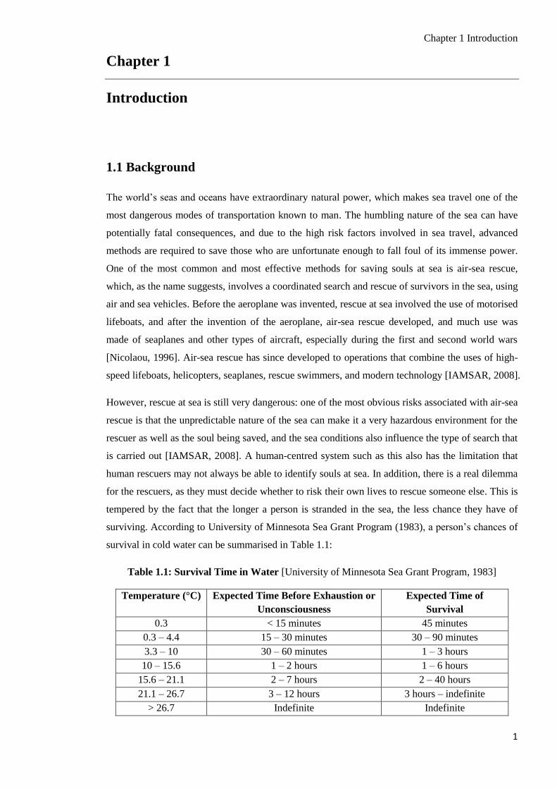
surviving. According to University of Minnesota Sea Grant Program (1983), a person’s chances of
survival in cold water can be summarised in Table 1.1:
Table 1.1: Survival Time in Water [University of Minnesota Sea Grant Program, 1983]
Temperature (°C) Expected Time Before Exhaustion or
Unconsciousness
Expected Time of
Survival
0.3 < 15 minutes 45 minutes
0.3 – 4.4 15 – 30 minutes 30 – 90 minutes
3.3 – 10 30 – 60 minutes 1 – 3 hours
10 – 15.6 1 – 2 hours 1 – 6 hours
15.6 – 21.1 2 – 7 hours 2 – 40 hours
21.1 – 26.7 3 – 12 hours 3 hours – indefinite
> 26.7 Indefinite Indefinite

Chapter 1 Introduction
2
From Table 1.1, it is clear that as the water gets colder, a person’s chances of survival decrease
rapidly. Consequently, the quicker someone is found, the more chance they have of surviving.
Keeping the rescue crew safe in adverse weather therefore decreases the chances of survival for
those waiting to be rescued.
One way of carrying out an effective search mission without putting rescuers in any danger, but at
the same time not wasting any time, is to employ an autonomous system involving a number of air
and sea vehicles. In this thesis, a single Unmanned Surface Vessel (USV) is used as the main hub,
and four autonomous Unmanned Aerial Vehicles (UAVs) are deployed from the deck of the USV
to search for survivors of a sinking ship in a given location. This allows a search to be carried out
without putting any other human lives in danger. The UAVs used are helicopters as opposed to
fixed-wing aircraft. The reason for choosing helicopters is that they have the ability to hover and
fly at low speeds, which enable them to follow precise trajectories [Thomson & Bradley, 1998] and
manoeuvre through tight spaces. This is an advantage for such a system because the space on the
surface vessel is limited, which makes helicopters more appropriate for deployment and capture.
When survivors are spotted in the sea, the information gained can be used to start unmanned or
manned rescue operations. The main benefits of using an autonomous system over a manned
system in this type of situation are that there is little risk to any rescuers, autonomous systems are
less likely to suffer from fatigue, they can gain and store more information than humans about an
environment using on-board sensors, and they are more accurate as they are not prone to human
error. There are however some limitations: the autonomous system is still subject to time
constraints due to fuel and power consumption. Therefore, the vehicles must be coordinated
efficiently to perform an effective search of the area.
The coordination of the autonomous vehicles involves generating appropriate commands to tell the
vehicles what locations to search. Instead of simply planning routes beforehand, some common
optimisation techniques are used to coordinate the vehicles. Optimisation techniques such as
Genetic Algorithms [Goldberg, 1989; Holland, 1992; Johnson & Picton, 1995; Mitchell, 1995;
Alfaro-Cid, 2003; Schmitt, 2004], Particle Swarm Optimisation [Eberhart & Kennedy, 1995;
Eberhart & Shi, 2001; Kennedy & Eberhart, 1995], Ant Colony Optimisation [Dorigo & Di Caro,
1999; Dorigo, Birattari & Stützle, 2006; Stützle & Hoos, 2000], Hill Climbing [Johnson & Picton,
1995; Russell & Norvig, 1995], Simulated Annealing [Johnson & Picton, 1995; Kirkpatrick, Gelatt
& Vecchi, 1983; Kirkpatrick, 1984; Russell & Norvig, 1995], and the simple Random Search
[Johnson & Picton, 1995; Karnopp, 1963], are commonly used to solve problems where the
problem space is too large to explore completely. These techniques are also useful when using
simple mathematical analysis is not practical due to the complex nature of the function being
optimised.

Chapter 1 Introduction
3
Carrying out a blind search for survivors in the sea is fundamentally different from the types of
problems commonly solved by these optimisation techniques given that the solutions are evaluated
by physically travelling to a point in space and taking measurements, rather than evaluating the
solutions almost instantly using pure computation. As well as this, there is a real time limit on the
search due to the fuel consumption of the UAVs. It is also different in the sense that other points in
the search space are visited en route to a given destination, which is not the case in other types of
problems. Also, many applications of these algorithms that involve searching for targets make use
of a-priori information about the search space, and some applications simply find optimal paths
around the search space by solving variations of the Travelling Salesman Problem [Johnson &
Picton, 1995], and conduct the search while following these paths. Another common method of
guiding autonomous vehicles is via artificial potential fields [Bennet & McInnes, 2010; McInnes,
2003; Park & Lee, 2003; Zhang, Chen & Fei, 2006], where each agent is modelled as a point in a
potential field with attraction towards some goal and repulsion from obstacles and threats. However,
this method is not suitable for this application, as this type of information about the search space is
not available beforehand. The main work carried out in this thesis involves testing the optimisation
techniques described above in the context of a blind autonomous air-sea search mission, and
developing these techniques to improve upon current air-sea search methods. The way in which
these optimisation techniques are applied to this problem is that they are used to generate a series
of waypoints for the agents to visit. The evaluation of each solution depends on what is detected at
that point.
1.2 Aims and Objectives
The aim of the research presented in this thesis is to design an autonomous, multi-vehicle system
capable of carrying out search missions at sea in order to detect survivors and rescue them. The
proposed system consists of four unmanned helicopters (UAVs) and a USV, and the aim is to
coordinate a search using common search algorithms/optimisation techniques. These search
algorithms are often used to solve combinatorial problems, so the main aim of this thesis is to
determine whether they can be used to carry out a successful search mission. This research also
aims to compare the performances of the optimisation techniques when two different objective
functions are used to drive the search. The objective functions are different in the sense that one of
them simply takes a temperature reading, and the other one also indicates the expected locations of
targets using a probability distribution, which updates throughout the search.
In order for these aims to be achieved, several objectives must be met first. The objectives for this
research are listed below:

Chapter 1 Introduction
4
Implement appropriate mathematical models of vehicles within a suitable simulation
environment
Design suitable navigation and control systems for vehicles
Develop a collision avoidance algorithm for multiple vehicles
Implement search algorithms into the autonomous guidance system to coordinate the
vehicles
The results in this thesis show that these objectives have been accomplished, and the search
algorithms have been applied successfully to the simulations of the autonomous air-sea rescue
system.
1.3 Contribution of Research
The research carried out in this thesis contributes to the areas of guidance and control, and also in
the application to autonomous search and rescue. The specific contributions of this work can be
summarised by the following list:
Design and comparison of PID and Sliding Mode controllers for the X-Cell 60 SE
helicopter
Application of common search algorithms to an autonomous air-sea rescue mission
Comparison of different objective functions used by the common search algorithms to
carry out the search
Development of effective hybrid methods in the context of autonomous air-sea rescue
Determination of the best algorithm for searching for survivors in the sea within a certain
time limit
Indication of best practice for autonomous air-sea search and rescue
This work contributes to control and guidance in terms of the application of certain control
algorithms to a specific model and the application of common search algorithms to a particular
kind of problem, which generally does not use this type of method. The main novel contributions of
the thesis are the development of effective hybrid methods that can be used to search for survivors
in the sea, and also the development of a probability distribution, which can be used to indicate
likely target locations.
To date, the following publications have resulted from the work carried out in this thesis:

Chapter 1 Introduction
5
Rafferty, K.J. and McGookin, E.W., (2012), “A Comparison of PID and Sliding Mode
Controllers for a Remotely Operated Helicopter”, 12th
International Conference on Control,
Automation, Robotics and Vision (ICARCV), Guangzhou, China, Dec 5-7, pp. 984-989
Rafferty, K.J. and McGookin, E.W., (2013), “An Autonomous Air-Sea Rescue System
Using Particle Swarm Optimization”, International Conference on Connected Vehicles and
Expo, Las Vegas, U.S.A., 2-6 Dec, pp. 459-464
1.4 Outline of Thesis
As stated previously, the main aim of this work is to determine whether common search algorithms
can be used to coordinate an autonomous air-sea search and rescue mission. The vehicles must be
controlled and guided efficiently so that they can carry out an appropriate search. The development
of the control and guidance strategies is presented in stages throughout the thesis. The theory and
implementation of the techniques are presented, and are then followed by the results of the
simulations.
Chapter 2 provides an overview of the relevant literature in the areas being studied in this thesis. In
particular, the literature is given for two established control techniques (PID and Sliding Mode),
and for the optimisation techniques discussed in Section 1.1. Also, current approaches employed
for manned search and rescue missions are discussed, as is the recent development of autonomous
Urban Search and Rescue systems.
Chapter 3 describes the mathematical model of the vehicles involved in the search mission: four
unmanned helicopters (all the same model) are used to carry out the search. A nonlinear
mathematical model of the helicopter is given, with the equations of motion representing the
dynamics of the vehicle as a whole, the dynamics of the main rotor blades (flapping and speed of
rotation), and the rotational transformations between the Earth-fixed frame and the helicopter body
frame. The actuator dynamics are also included.
Chapter 4 presents the navigation and control implications for this type of application. In terms of
navigation, the line-of-sight autopilot is introduced. A strategy for collision avoidance is also
introduced, and uses the concept of a collision cone. In terms of control, the theories behind PID
control and Sliding Mode Control are given in some detail, as are the methods of implementing
these controllers. Results are then shown for several simulations involving these controllers.
Chapter 5 discusses the theory of several search algorithms that are applied to the autonomous air-
sea rescue system. In particular, a background is given on three common search patterns used in
real search missions, and the theory behind a number of common optimisation techniques is given.

Chapter 1 Introduction
6
Chapter 6 presents the simulation results for most of the basic search algorithms discussed in
Chapter 5. The results from each algorithm and search scenario are presented graphically and
analysed in terms of performance.
Chapter 7 introduces the probability distribution that is used to further guide the searches. The
optimisation techniques that are discussed in Chapter 5 are tested with the inclusion of this
probability distribution. Again, the results from each algorithm and search scenario are presented
graphically and analysed in terms of performance.
Chapter 8 shows the simulation results for hybrid algorithms developed from the optimisation
techniques discussed in Chapter 5. Naturally these hybrid techniques are evaluated and results
analysed in the same way as the pure heuristics considered in Chapters 6 and 7.
Chapter 9 concludes the thesis by giving a summary of each chapter and the conclusions that have
been drawn from the presented research. Some ideas for areas of possible future work are given at
the end of this chapter.
Chapter 2 Literature Review
7
Chapter 2
Literature Review
2.1 Introduction
This chapter presents a review of the relevant literature related to the work carried out in this thesis.
The work presented here is based on simulations of an autonomous system carrying out an air-sea
rescue mission. The system involves an Unmanned Surface Vessel (USV), from which four rotary
Unmanned Aerial Vehicles (UAVs) are deployed. All four UAVs are then used to search for
survivors from stricken ocean vessels in the sea. In order for this system to be simulated, many
different fields of research have to be fused together.
An essential part of any autonomous system is the control of the vehicles involved. In this
particular case, the UAVs must be controlled accurately so that they can effectively execute the
search mission in the desired manner. Two different control methodologies are tested in this thesis:
PID Control and Sliding Mode Control. These control methodologies are both presented in this
chapter, along with a review of the literature.
The use of robots in Urban Search and Rescue (USAR) has been a major research area for over a
decade, and is related in many ways to autonomous air-sea rescue. A review of the literature on
autonomous USAR is therefore presented. In the context of this thesis, in order to provide a
benchmark for the autonomous air-sea search, a study of some of the standard search patterns used
in manned air-sea rescue is carried out. Descriptions of some of these standard techniques are
presented, as are the situations where they are applied.
Since the main aim of the research is to investigate various strategies for an autonomous search
mission, a literature review of several search algorithms is also carried out. The search algorithms
applied to the simulations are commonly used as optimisation techniques for combinatorial
problems. However, their effectiveness in the context of an autonomous search mission is
investigated in this thesis. A review of the literature on these optimisation techniques is therefore
presented.
The review of the state of the art in each of the research areas in this study is carried out in this
chapter. Section 2.2 presents an overview of the control methodologies used. Section 2.3 discusses
the development of autonomous USAR, as well as some of the standard search techniques used in
real-life maritime search and rescue. Section 2.4 reviews the relevant literature for each of the

Chapter 2 Literature Review
8
optimisation techniques and their applications. Finally, Section 2.5 provides a brief summary of
this chapter.
2.2 Control Methodologies
Controlling a system amounts to using inputs to maintain certain variables at their desired values,
just like a driver controls a car by applying appropriate inputs to the steering wheel, pedals, and
gears to maintain an appropriate direction, speed, and rev count. There is a considerable amount of
literature on feedback control [Franklin, Powell, & Emami-Naeini, 1991; Philips & Harbor, 1996;
Skogestad & Postlethwaite, 2007], which uses feedback from sensors, so that the control inputs can
be adjusted accordingly. This thesis investigates two well-known types of feedback control:
Proportional-Integral-Derivative Control (PID Control) [Åström & Hägglund, 1995; Franklin et al,
1991; Wang, Ye, Cai & Hang, 2008], and Sliding Mode Control [Bag, Spurgeon & Edwards, 1996;
Edwards & Spurgeon, 1998; Spurgeon, Edwards and Foster, 1996; Utkin, Guldner & Shi, 1999;
Young, Utkin and Ӧzgüner, 1999]. The reason for choosing these methods is that they are well-
established and very popular.
2.2.1 PID Control
PID Control [Åström & Hägglund, 1995; Dutton, Thompson & Barraclough, 1997; Franklin et al,
1991; Wang et al, 2008] is a very popular control method because conceptually, it is simple and is
easy to implement yet it is effective. An excellent introductory text on PID Control is the text by
Åström & Hägglund (1995), which provides background theory, implementation issues, and many
examples. In fact, according to Åström & Hägglund (1995), PID control is used in more than 95%
of processes. Although this statement was made in the 1990s, it does illustrate how popular this
particular control methodology really is. Even today, a search on PID control will reveal numerous
articles on the theory and many different types of applications. Another text which provides a fairly
comprehensive treatment of PID control, including design methods and applications, is Wang et al
(2008).
A PID controller is commonly referred to as a three term controller due to the proportional, integral
and derivative elements that make up its fundamental structure [Åström & Hägglund, 1995; Dutton
et al, 1997]. The parameters of a PID controller are the three gains, which determine the
contribution from each of the proportional, integral and derivative terms. Since this is really all
there is to PID control, it is not surprising that many different techniques have been developed over
the years to find appropriate gains. The gains can be tuned using a trial and error approach [Åström
& Hägglund, 1995; Alfaro-Cid, 2003], but they can also be tuned using more mathematical

Chapter 2 Literature Review
9
approaches, the most popular of which is the Ziegler-Nichols method [Ziegler & Nichols, 1942].
The original paper on this method was written by Ziegler and Nichols in 1942, and has been
discussed in the literature since then. Although the Ziegler-Nichols method gives a “formula” for
the gains, it is generally accepted that the resulting gains often require slight adjustments in order to
achieve desired performance [Ogata, 2002; Franklin et al, 1991]. Appropriate gains may also be
determined using automatic tuning; Hägglund & Åström (1991) describes several adaptive
techniques for tuning the gains by investigating the frequency response of the system.
Many pieces of literature present applications of PID control, including Li & Li (2011), Sakamoto,
Katayama & Ichikawa (2006), and Xiao, Zou & Wei (2010). An example of a PID controller
applied to a small helicopter can be found in Castillo, Alvis, Castillo-Effen, Moreno & Valavanis
(2005).
2.2.2 Sliding Mode Control
Sliding Mode Control [Edwards & Spurgeon, 1998; Utkin et al, 1999; Young et al, 1999] is a type
of Variable Structure Control [Edwards & Spurgeon, 1998], which was developed from work
carried out in Russia during the early 1960s, and became known outside Russia in the 1970s
[Edwards & Spurgeon, 1998]. Sliding Mode controllers, by the very nature of their design, are
capable of rejecting disturbances and coping with model uncertainty [Young et al, 1999]. It is
therefore considered to be a better and more robust controller than a PID controller when it comes
to controlling dynamic nonlinear systems.
The main problem with the basic version of Sliding Mode control is a phenomenon known as
chattering [Edwards & Spurgeon, 1998; McGookin, 1997; Utkin et al, 1999], which is high-
frequency changes in the desired control input. Sliding Mode control is an example of variable
structure control, which means the control law can change depending on the state of the system. As
there is a discontinuity in the control law between different states, the result is that the desired
control input can change rapidly in certain situations, which causes unnecessary wear and tear of
the actuators. Specifically, this occurs as the system switches from one side of the sliding surface
[Edwards & Spurgeon, 1998] to the other. There are a variety of methods of reducing the chattering
effect, the most common of which is to replace the discontinuity with a smooth transition between
the different control laws over a finite boundary layer [Healey & Lienard, 1993; Utkin et al, 1999;
Young et al, 1999]. Utkin et al (1999) presents and compares several methods (including the
boundary layer method) for eliminating chattering, and describes the different scenarios that are
most suitable for each method. Another more recent idea for eliminating chattering can be found in
Tseng & Chen (2010), where an integrator is placed in front of the system, and a normal Sliding

Chapter 2 Literature Review
10
Mode controller is designed for this augmented system. This eliminates chattering as the integrator
acts as a low pass filter.
As it is a popular control method, Sliding Mode Control can be found in many pieces of literature.
Two of the most popular texts are Edwards & Spurgeon (1998), and Utkin et al (1999), which
explain the theory in great detail and give numerous examples. There are many other sources that
describe applications of Sliding Mode control: literature for maritime applications includes Healey
& Lienard (1993), and Fossen (1994), and helicopter flight control applications can be found in
Bag et al (1996), and Spurgeon et al (1996).
2.3 Search and Rescue
2.3.1 Autonomous Urban Search and Rescue
Since the turn of the century, mobile robots have become extremely useful resources in USAR due
to their ability to search unknown areas that are hazardous or even inaccessible to rescue workers
[Liu & Nejat, 2013]. There are many advantages of using robots in USAR: unlike rescue workers,
they are not affected by stress or fatigue [Burke, Murphy, Coovert & Riddle]; robots can be made
in large quantities whereas human rescue workers are not as readily available [Casper & Murphy,
2003]; damaged robots can be easily repaired or replaced whereas the loss of a human life has a
much greater impact on society [Casper, Micire & Murphy, 2000]. Due to these obvious benefits,
the use of mobile robots in USAR has become a significant research topic in the last decade [Liu &
Nejat, 2013].
The development of rescue robots was motivated by two major disasters: the Kobe earthquake in
Japan in 1995 and the Oklahoma City bombing in 1996 [Murphy, Tadokoro, Nardi, Jacoff, Fiorini,
Choset & Erkmen, 2008]. Since the turn of the century, robots have been utilised in many USAR
operations. The first known application of robots in USAR was in the aftermath of the World Trade
Centre disaster on September 11th 2001 [Murphy, 2004]. Since then, mobile robots have
participated in USAR operations of many other disasters, such as Hurricanes Katrina, Rita, and
Wilma in the U.S.A. in 2005 [Murphy et al, 2008], the Haiti earthquake in 2010 [Guizzo, 2011],
and the Tohoku earthquake and tsunami in Japan in 2011 [Guizzo, 2011].
One of the main challenges associated with autonomous USAR is that disaster sites are often
highly cluttered, which makes it very difficult for robots to navigate the site and search for
survivors without a human in the loop [Liu & Nejat, 2013]. However, this has its own problems, as
humans may have difficulties in determining the true nature of the environment from remote visual
feedback [Liu & Nejat, 2013], and this can result in robots becoming physically stuck [Casper &
Murphy, 2003]. Therefore, one of the main aims of robotics research is to improve low-level

Chapter 2 Literature Review
11
autonomy, such as controlling robots for the purpose of navigation through rough terrain [Mourikis,
Trawny, Roumeliotis, Helmick & Matthies, 2007; Okada, Nagatani, Yoshida, Tadokoro, Yoshida
& Koyanagi, 2011], and also being able to map an USAR environment [Kurisu, Muroi, Yokokohji
& Kuwahara, 2007; Zhang, Nejat, Guo & Huang, 2011]. There has also been a great deal of
research in the development of semi-autonomous control [Wegner & Anderson, 2006; Doroodgar,
Ficocelli, Mobedi & Nejat, 2010], which can provide a balance between teleoperation and low-
level autonomy. This type of balance is very useful as it allows the operator to concentrate on
higher-level tasks such as supervision of multiple robots and specifying the direction of travel [Liu
& Nejat, 2013], and has thus paved the way for the development of single-human multi-robot
systems. Such systems are more cost-effective than single-human single-robot systems [Liu &
Nejat, 2013], and therefore, a great deal of research has been done on the development of such
systems, with much emphasis being placed on teamwork among the robots themselves, and also
between robots and humans [Sato, Matsuno, Yamasaki, Kamegawa, Shiroma & Igarashi, 2004;
Luo, Espinosa, Pranantha & De Gloria, 2011]. The development of autonomous USAR systems in
recent years has certainly proved to be very promising, but there are still more challenges that lie
ahead, including the development of robotic systems that can transport trapped victims to safety
[Yim & Laucharoen, 2011], and therefore, autonomous USAR promises to be a very exciting
research area in the coming years.
While the contribution of this thesis is in the development of autonomous air-sea rescue rather than
autonomous USAR, the methodologies are certainly transferrable to USAR. This thesis aims to
determine whether optimisation techniques can be applied to autonomous air-sea rescue so that a
search can be carried out in a structured and controlled manner, and extends on the work carried
out by Worrall (2008) by introducing several hybrid algorithms.
2.3.2 Standard Maritime Search and Rescue Techniques
Currently, the standard procedures carried out in air-sea search and rescue operations can be found
in the International Aeronautical and Maritime Search and Rescue (IAMSAR) manual [IAMSAR,
2008]. In particular, the standard search approaches are outlined in Volume II, Mission co-
ordination. Some of the most common search patterns used are the Parallel Sweep Search, Sector
Search, and Expanding Square Search.
The Parallel Sweep Search simply sweeps back and forward along the long sides of a rectangle,
moving part of the way along the smaller side between each sweep. The search can be carried out
with multiple vehicles by assigning each vehicle to separate sub-regions. This technique is often
used when there is a large uncertainty in the target locations [IAMSAR, 2008], and is very effective
at searching areas with uniform coverage. This technique is described in more detail in Chapter 5.

Chapter 2 Literature Review
12
The Sector Search is used to search a circular area about some point. The search starts at the centre
and travels to the edge of the circle, then turns 120° starboard, then keeps on searching, turning
120° starboard every time it reaches the edge of the circle. Consequently, this particular search
gives good coverage nearer the centre of the circle, and is very effective when target locations are
known reasonably well and also when the search area is small [IAMSAR, 2008]. Like Parallel
Sweep, this technique is described in more detail in Chapter 5.
The Expanding Square Search starts at the centre of a given region, and then travels around the
centre point in a square pattern, with the length of the square expanding after every two sides, so
that the search covers the area around the centre in a uniform manner. Like the Sector Search, this
technique is often most effective when the target locations are known reasonably well [IAMSAR,
2008]. Again, this technique is described in more detail in Chapter 5.
There are many other search techniques, and various criteria for using each particular search
method. As mentioned, more details on these search methods can be found in the IAMSAR manual
[IAMSAR, 2008]. In this thesis, the three techniques described above provide a benchmark for
more complex heuristic techniques in an air-sea search mission, where the heuristic techniques are
developed from existing optimisation methods, which are not normally used in this context.
2.4 Optimisation Techniques
The optimisation techniques described in this section are used as search methods for the air-sea
rescue mission. These optimisation techniques are commonly used to solve combinatorial problems
when the search space is too large to evaluate every possible solution within a reasonable time and
also when using simple mathematical analysis is not practical or even possible. The reason for
using these optimisation techniques in this thesis is that the task of searching for survivors in the
sea can be considered an optimisation problem, where the optimal solutions are the locations of the
survivors. Given that the search space is too large to search exhaustively, it is appropriate to use
such optimisation techniques, and this thesis aims to determine whether these techniques are
effective in the context of an autonomous air-sea search mission. This section gives a brief
overview of these optimisation techniques, and their common applications. The techniques are then
described in more detail in Chapter 5.
2.4.1 Random Search
The Random Search [Johnson & Picton, 1995; Karnopp, 1963] is one of the simplest optimisation
techniques. The algorithm proceeds by simply selecting random points in the search space and

Chapter 2 Literature Review
13
evaluating them, without using any information from previous points. Because this algorithm is so
simple, there is not much literature on the theory. However, there is some literature on robotic
applications of Random searches, such as Rybski, Larson, Veeraraghavan, LaPoint & Gini (2007),
and Suzuki & Żyliński (2008). From these papers, it can be inferred that the main advantage of
Random searches is the resulting unpredictability and diversity, which is often required to achieve
positive results. The Random Search is also discussed in Worrall (2008), with applications to
USAR, and it is shown that the Random Search covers a lot of ground even without any memory.
A similar approach is used in this thesis in the context of air-sea rescue, and is used as a benchmark
for more complex techniques.
2.4.2 Hill Climbing
The Hill Climbing algorithm [Johnson & Picton, 1995; Russell & Norvig, 1995] is a local-search
algorithm [Rayward-Smith, Osman, Reeves & Smith, 1996], which uses information from the best
of the previous evaluations to generate other candidate solutions. Basically, at each iteration, the
algorithm seeks a solution close to the current solution, and accepts the new solution if it is an
improvement on the current solution. It is also common to introduce Random Restart when no
progress is made after a certain length of time [Russell & Norvig, 1995; Worrall, 2008], as this
gives the algorithm a better chance of covering a larger portion of the search space and prevents it
from getting stuck at local optima, as discussed in Chapter 5.
The theory of the Hill Climbing algorithm can be found in Johnson & Picton (1995), and Russell &
Norvig (1995). Applications of the Hill Climbing algorithm include optimising the time to
assemble components on a printed circuit board [Filho, Costa, Filho, & de Olieira, 2010], finding
optimal configurations for web application servers [Xi, Liu, Raghavachari, Xia & Zhang, 2004],
organising sporting tournaments [Lim, Rodrigues & Zhang, 2006], and pursuing mobile targets
using unmanned aerial vehicles [Zengin & Dogan, 2007]. Hill Climbing has also been applied to
search and rescue by generating optimal paths based on a generalisation of the Travelling Salesman
Problem, which involves finding the shortest route round a series of cities: an application of this
type can be found in Jacobson, McLay, Hall, Henderson & Vaughan (2006). In this thesis, Hill
Climbing is used to conduct a blind search in the context of air-sea rescue. Worrall (2008)
considers this in the context of USAR, but this type of application is relatively uncommon.
2.4.3 Simulated Annealing
Simulated Annealing [Johnson & Picton, 1995; Kirkpatrick et al, 1983; Kirkpatrick, 1984; Russell
& Norvig, 1995] is based on the physical process of annealing [Kirkpatrick et al, 1983], which is

Chapter 2 Literature Review
14
the cooling process in materials. In order to carry out this process, the substance is melted and then
the state of the substance is perturbed (i.e. the atoms are given a small random displacement,
resulting in a change in energy) as the temperature is gradually decreased, until it solidifies when it
reaches its ground state [Kirkpatrick et al, 1983]. Metropolis, Rosenbluth, Rosenbluth, Teller &
Teller (1953) devised Simulated Annealing: an optimisation technique which mimics this cooling
process. Simulated Annealing is very similar to Hill Climbing, in that it conducts a local search
about some current solution. The one main difference is that the Simulated Annealing algorithm
sometimes accepts new solutions that are poorer than the current solution. The procedure of
deciding whether to choose a poorer solution is known as the Metropolis Procedure [Kirkpatrick et
al, 1983], and mimics the probability of a collection of atoms jumping to a higher energy level,
which is determined by a Boltzmann probability factor [Kirkpatrick et al, 1983; Metropolis et al,
1953]. This is discussed in more detail in Chapter 5
The original idea of Simulated Annealing can be found in Metropolis et al (1953), but due to the
significant calculations involved, the first real investigation was not carried out until the 1980s. The
paper by Kirkpatrick et al (1983) investigates the impact of using Simulated Annealing to find
optimal solutions to the Travelling Salesman Problem. This work shows the benefits of using
Simulated Annealing to solve such optimisation problems. The theory of Simulated Annealing can
be found in texts such as Johnson & Picton (1995), and Russell & Norvig (1995). There are various
other successful applications of Simulated Annealing, such as solving the quadratic assignment
problem [Wilhelm & Ward, 1987], constructing school timetables [Abramson, 1991], and
organising sporting tournaments [Lim et al, 2006]. From an aerospace point of view, Simulated
Annealing has been used as a method to optimise control parameters [Martinez-Alfaro & Ruiz-
Cruz, 2003; McGookin & Murray-Smith, 2006] and has also been tested on air traffic control and
aircraft mission planning problems with positive results [Jackson & McDowell, 1990]. More
recently, Simulated Annealing has been used successfully to find optimal or near-optimal paths for
mobile robots in dynamic environments [Miao & Tian, 2008], but like Hill Climbing, using
Simulated Annealing for blind searches is uncommon.
2.4.4 Genetic Algorithms
Genetic Algorithms [Goldberg, 1989; Holland, 1992; Johnson & Picton, 1995; Mitchell, 1995;
Alfaro-Cid, 2003; Schmitt, 2004] are nature-inspired optimisation techniques, which mimic the
biological process of natural selection and evolution [Mitchell, 1995]. In nature, organisms evolve
through the processes of natural selection, crossover and mutation [Holland, 1992]. A Genetic
Algorithm is essentially a mathematical model of this “survival of the fittest” process, where a
population of solutions evolves through a number of generations by these natural operators, and
only the best solutions survive to the end.

Chapter 2 Literature Review
15
The original theory of Genetic Algorithms was developed by John Holland in the 1960s, and the
theory was then described in Holland (1975). The popularity of this method then increased in the
mid-1980s: a paper by Grefenstette (1986) provides an investigation and comparison of the various
parameters associated with Genetic Algorithms such as population size, mutation rate and selection
method. Several interesting observations are made: for example, high mutation rates can be
harmful with respect to online performances, and rank-based selection methods outperform those
that are probability based. The book by Goldberg (1989) discusses the theory and applications of
Genetic Algorithms, and is still considered a popular source on the subject today.
Since the late 1980s, there has been much literature published on the theory and applications of
Genetic Algorithms. Another good source for the theory of Genetic Algorithms, including a
mathematical analysis of why they work (known as the Schema Theorem) is Mitchell (1995). This
paper also describes in detail the application of Genetic Algorithms to the Prisoner’s Dilemma
[Axelrod, 1987; Goldbeck, 2002], which was investigated by Axelrod in 1987. This “game” is
between 2 people, and involves the dilemma for each player of whether to “cooperate” or “defect”:
if one player defects and the other cooperates, the player who defects gets a high reward, but the
dilemma is that if both players defect, the end result is worse than if they both cooperate. Axelrod
found that the best strategies are typically variations of “Tit for Tat”, where each player punishes
defection and rewards cooperation. Another common application of Genetic Algorithms is
optimising control parameters, with numerous sources showing successful applications [Alfaro-Cid,
2003; Goh, Gu & Man, 1996; McGookin, Murray-Smith & Li, 1997; McGookin, Murray-Smith, Li
& Fossen, 2000]. Like Simulated Annealing, Genetic Algorithms have also been applied
successfully to the Travelling Salesman Problem [Bryant & Benjamin, 2000; Dwivedi, Chauhan,
Saxena & Agrawal, 2012; Homaifar, Guan & Liepins, 1992; Wei & Lee, 2004].
There are many variations associated with Genetic Algorithms due to the number of different
possibilities in each natural operator, and these variations can be found in the literature. For
example, many different selection methods exist, the most common of which are Elitist [Dwivedi et
al, 2012; McGookin et al, 1997], Roulette Wheel [Goldberg, 1989; Rayward-Smith et al, 1996],
and Tournament Selection [Miller & Goldberg, 1995; Rayward-Smith et al, 1996], as discussed in
Chapter 5.
Many different forms of the crossover operation have also been suggested in the literature: this is
where two parent solutions exchange certain characteristics to form two child solutions for the next
generation. Examples of common crossover techniques are single-point crossover [Mitchell, 1995;
Khoo & Suganthan, 2002], two-point crossover [Khoo & Suganthan, 2002; McGookin, 1997;
Worrall, 2008], uniform crossover [Khoo & Suganthan, 2002], multi-point crossover [De Jong &
Spears, 1992] and gene-lottery [Schmitt, 2004]. Single-point and two-point crossover are discussed
in Chapter 5.

Chapter 2 Literature Review
16
After crossover comes the process of mutation [Holland, 1975; Khoo & Suganthan, 2002;
McGookin, 1997], where parts of the child solutions are altered probabilistically. With a high
mutation rate the search tends to be more diverse but possibly at the expense of losing good
solutions. Conversely a low mutation rate keeps the basic structure of the Genetic Algorithm but
possibly at the expense of getting stuck in a locally optimal candidate solution. Although the
mutation rate is usually kept constant throughout a search, it has been shown that it can be
beneficial to start with a high mutation rate and lower it throughout the search, so that the search is
more diverse at the start, and then hones in on the good solutions and keeps them as the simulation
goes on [Khoo & Suganthan 2002; Yaman & Yilmaz, 2010].
This thesis uses Genetic Algorithms to carry out a blind search for air-sea search and rescue. Again,
Worrall (2008) considers this approach for USAR, and shows that Genetic Algorithms can be used
in this context. However, this type of application is uncommon, and indeed, most applications to
search and rescue are based on variations of the Travelling Salesman Problem, where agents are
required to find optimal paths, as in Arulselvan, Commander & Pardalos (2007), Davies & Jnifene
(2006), and Giardini & Kalmár-Nagy (2006).
2.4.5 Particle Swarm Optimisation
Particle Swarm Optimisation [Eberhart & Kennedy, 1995; Eberhart & Shi, 2001; Kennedy &
Eberhart, 1995] is an optimisation technique, which, like Genetic Algorithms, is inspired by nature.
In particular, the method emerged after attempting to simulate the flocking of birds. The original
idea was to simulate various characteristics of bird flocking, such as changing direction very
quickly, yet regrouping and maintaining a structured pattern. This optimisation technique is similar
to Genetic Algorithms in the sense that a population of solutions (particles) is given random
starting points, and they all cooperate to find new generations of solutions, but the way in which
this is done is different here: in Particle Swarm Optimisation, the “particles” are effectively flown
through the search space, and each particle is given a velocity such that it accelerates towards the
best solutions [Eberhart & Shi, 2001].
Particle Swarm Optimisation was developed in the mid-1990s by Kennedy & Eberhart (1995): this
paper describes the many variations that were tested during the development of the original version
of the algorithm. The paper includes descriptions of concepts such as nearest neighbour velocity
matching, craziness and the cornfield vector, as discussed in Chapter 5. Many of these concepts
were found to be superfluous to the optimisation algorithm, and were eliminated as a result
[Eberhart & Shi, 2001; Kennedy & Eberhart, 1995]. The original version of the algorithm involves
a group of agents/particles, each with a certain number of dimensions, and each particle is given a
velocity (with the same number of dimensions as the particle) and a position, which corresponds to

Chapter 2 Literature Review
17
a “solution”. This is updated at each iteration based on the best solutions found by each particle,
and also the best solution found overall.
Some modifications to the original particle swarm optimisation algorithm were then suggested,
such as the inertia weight [Eberhart & Shi, 2000; Eberhart & Shi, 2001; Shi & Eberhart, 1998] and
the constriction factor [Clerc, 1999; Clerc & Kennedy, 2002; Eberhart & Shi, 2000]. The inertia
weight is a parameter designed to provide better control of exploration and exploitation [Eberhart
& Shi, 2001; Shi & Eberhart, 1998], and the constriction factor is designed to aid convergence
[Clerc & Kennedy, 2002; Eberhart & Shi, 2001]. Another modification that had to be made to the
algorithm was a way to incorporate constraints into the procedure, using methods such as
introducing a penalty function [Parsopoulos & Vrahatis, 2002], or ignoring unfeasible solutions
[Hu, Eberhart & Shi, 2003]. However, the basic idea of particles flying through the search space
remains constant throughout all this development.
Applications of Particle Swarm Optimisation include optimising electrical power systems [Yoshida,
Fukuyama, Takayama & Nakanishi, 1999], alignment of optical fibres [Landry, Kaddouri,
Bouslimani & Ghribi, 2012], and optimising neural networks [Carvalho & Ludermir, 2007].
Particle Swarm Optimisation has also been used to navigate robots by determining optimal paths
[Ahmadzadeh & Ghanavati, 2012], and has also been applied to searching for targets in unknown
environments [Derr & Manic, 2009; Rafferty & McGookin, 2013]. Derr & Manic (2009) carry out
an experiment with multiple targets that emit radio frequency signals, which are detectable by the
robots. It was found that Particle Swarm Optimisation is effective in this scenario, but system noise
could affect the received signal strength and hence the time taken to find targets. In Rafferty &
McGookin (2013), Particle Swarm Optimisation is used to simulate UAVs searching for humans in
the sea, and it was found that this algorithm performs better on average than a basic Random
Search.
2.4.6 Ant Colony Optimisation
Ant Colony Optimisation [Dorigo & Di Caro, 1999; Dorigo et al, 2006; Stützle & Hoos, 2000] is
an optimisation technique, which takes inspiration from the way in which colonies of ants
communicate with each other by depositing pheromones, and find favourable paths towards food
sources. The inspiration for Ant Colony Optimisation came from experiments performed by Goss,
Aron, Deneubourg, & Pasteels (1989), and Deneubourg, Aron, Goss & Pasteels (1990) involving a
colony of ants and a food source, with the path from the nest to the food source being a choice of
two bridges. In the experiment by Goss et al (1989), the two bridges are different lengths and after
time, the ants eventually choose the shorter one; in the experiment by Deneubourg et al (1990), the
bridges are the same length, and due to random fluctuations, the ants eventually began to favour

Chapter 2 Literature Review
18
one bridge, although after repeating the experiment several times, it was found that each bridge was
favoured about 50% of the time. Optimisation techniques based on the behaviour of ants were then
proposed in the early 1990s [Dorigo, Maniezzo & Colorni, 1991; Dorigo, 1992], and the Ant
Colony Optimisation technique developed from there.
Ant Colony Optimisation is an iterative process, and at each stage, every ant deposits a certain
amount of pheromones to indicate the quality of the path it has taken. The ants can sense nearby
pheromones and are naturally drawn towards areas where the pheromone concentration is high
[Dorigo et al, 2006]. Over time, pheromones evaporate if none are deposited for any length of time.
Therefore, when a favourable path is chosen, the pheromone strength increases, which increases the
probability of other ants choosing that path, which increases the pheromone strength again until
eventually, all the ants follow that path.
The basic theory of Ant Colony Optimisation, as well as a summary of different variations and
applications can be found in Dorigo et al (2006), which also gives an example of the application of
Ant Colony Optimisation to the Travelling Salesman Problem. In fact, the Travelling Salesman
Problem is a very common application of Ant Colony Optimisation, and many papers have been
published on this [Dorigo & Gambardella, 1997; Dorigo et al, 2006; Dorigo, Maniezzo & Colorni
1996; Stützle & Hoos, 2000]. Other successful applications of Ant Colony Optimisation include
routing problems in telecommunication networks [Schoonderwoerd, Holland, Bruten & Rothkrantz,
1996], project scheduling [Merkle, Middendorf & Schmeck, 2002], and finding optimal solutions
for robotic path planning problems [Ma, Duan & Liu, 2007; Zhang, Wu, Peng & Jiang, 2009]. The
paper by Parunak, Purcell & O’Connell (2002) applies a digital pheromone concept to the
coordination of swarming UAVs, with each specific location in the search space having a particular
pheromone level, rather than having pheromones along the edges that connect different points. The
results from this paper indicate that this technique is suitable for coordinating UAV swarms. This
version is similar to that tested in this thesis.
Another nature-inspired algorithm that is becoming increasingly popular is Bacterial Foraging
Optimisation [Das, Biswas, Dasgupta & Abraham, 2009; Niu, Fan, Tan, Rao & Li, 2010; Passino,
2002; Liu & Passino, 2002]. This algorithm is based on the foraging behaviour of bacteria such as
E.coli as they search for nutrients [Passino, 2002]. Based on this foraging behaviour, the Bacterial
Foraging Optimisation algorithm was proposed in 2002 by Passino, and has become increasingly
popular over the last decade. However, this algorithm has not been applied to the simulations in
this thesis, as it is felt that it is not suitable for the particular simulations being carried out. There
are two main reasons for this: firstly, based on the algorithm description in Passino (2002), each
bacterium (and hence, each agent in this case) takes turns to evaluate several solutions. This is
practical if solutions can be evaluated instantly (or very quickly) but in this case, it would be
impractical because it takes time for the agents to travel to their “solutions” and hence, a lot of time

Chapter 2 Literature Review
19
would be wasted. The second reason is that given the time constraints imposed by fuel
consumption, the algorithm would not get a chance to develop and as a result, the algorithm would
behave in a similar way to the Hill Climbing algorithm, as the start of the algorithm is similar to
this method. Therefore, Bacterial Foraging Optimisation has not been applied to the simulations.
2.5 Summary
This chapter provided a review of some of the literature associated with the main topics discussed
in this thesis. The main topics discussed are control methodologies, the development of USAR
operations, the standard patterns for maritime search and rescue operations, and optimisation
techniques. The main focus of this thesis is the application of optimisation techniques to an
autonomous system for air-sea rescue, with the emphasis being on the coordination of a group of
agents to detect targets.
Although various control methodologies have been used for helicopter control, two specific control
methodologies were discussed: PID Control and Sliding Mode Control. A brief background of PID
Control was presented, as was key literature describing the theory and some applications of this
technique. Methods of tuning the gains were also discussed, and the relevant literature was given.
Sliding Mode Control was then discussed in terms of origin, theory and applications, along with the
relevant literature.
Next, an overview of the development of autonomous USAR was presented, as well as the
challenges associated with this. Then, three standard search patterns for maritime rescue were
discussed: Parallel Sweep, Sector Search, and Expanding Square. A brief description of the theory
and effectiveness of each technique was given, as was the main source of information about them.
Finally, several optimisation techniques were introduced, along with relevant literature. First of all,
two basic algorithms were discussed: Random Search, and Hill Climbing. Next, Simulated
Annealing was presented, along with the literature that describes the inspiration for this technique
and the development of it. Then, three biologically-inspired techniques were discussed: Genetic
Algorithms, Particle Swarm Optimisation, and Ant Colony Optimisation, which are designed to
mimic natural processes. i.e. evolution, the flocking of birds, and path coordination in ants. The
literature describing the original development of these algorithms was presented, as well as a basic
account of the theory of each of these techniques. Several applications of each technique were
presented, including applications relevant to the work being carried out in this thesis. A brief
description of the theory and development of another popular biologically-inspired algorithm was
then presented: Bacterial Foraging Optimisation. However, as explained, this method is not used in
this thesis because it would not get a chance to develop properly and it would behave in a similar
way to Hill Climbing.

Chapter 3 mathematical Model
20
Chapter 3
Mathematical Model
3.1 Introduction
Simulations are very useful for testing real systems [Murray-Smith, 1995], for reasons such as cost,
time, safety, practicality, and the ability to test the system under specified conditions. The process
of testing a physical system can be very costly and time-consuming, not to mention dangerous and
impractical. This is especially true if there are multiple vehicles involved. Also, random changes in
the environment such as wind speed and temperature can be controlled during simulations,
meaning that fair comparisons can be made between various aspects of the simulations.
In order to run an appropriate simulation, an accurate mathematical model of the system is required,
so that the system being simulated is a realistic representation of the actual system [Murray-Smith,
1995]. A mathematical model of a physical robotic system typically consists of a set of differential
equations that represent the system. These equations of motion describe the position, orientation,
and movement of the system, and often of various subsystems as well [Cannon, 2003]. The
equations of motion can be separated into kinematics and dynamics. The kinematics describes the
geometry of the motion, and is represented by a transformation between two reference frames, one
of which is an inertial reference frame: in this case, the kinematic equations represent the
transformation between the Earth-fixed inertial frame and the body-fixed frame of the helicopter.
The dynamics describe the forces and moments that act on the system, and how the system reacts to
these forces and moments, as opposed to the kinematics, which describe only the geometry of the
motion and not the cause of the motion. The effects of gravity on the system are an example of
dynamics. Gravity causes a downward force (more specifically, towards the centre of the Earth) on
a system, so for example, a helicopter must produce an upward thrust to balance this. This force is
provided by the main rotors. The upward force on a boat is provided by the upthrust, which is an
upward force generated when the boat is placed in water. Another example of dynamics is the
effect of air resistance: when a helicopter moves relative to the air, this causes a resistive force,
which opposes the movement of the helicopter.
Section 3.2 of this chapter describes the dynamics of the helicopter, and expands on the definition
of the key forces and moments that act on the helicopter. Section 3.3 describes the basic kinematics
of the helicopter, including details of the rotational transformations. Section 3.4 discusses the
nonlinear actuator dynamics of the helicopter. In Section 3.5, the process of linearizing a nonlinear

Chapter 3 mathematical Model
21
mathematical model is presented, and the advantages of this representation are discussed. Finally,
Section 3.6 summarises the chapter.
3.2 Helicopter Dynamics
3.2.1 Rigid Body Dynamics
The helicopter used to simulate the autonomous air-sea search mission is the X-Cell 60 SE
helicopter [Budiyono, Sudiyanto & Lesmana, 2007; Gavrilets, 2003; Karasu, 2004]: a miniature
helicopter, as shown in Figure 3.1. This particular helicopter model was used because of the
availability of the full mathematical model. The parameters of this helicopter, along with
appropriate descriptions, are shown in Table (3.1).
Figure 3.1: X-Cell 60 SE Helicopter [Gavrilets, 2003, © MIT]
The dynamics of the X-Cell 60 SE helicopter [Budiyono et al, 2007; Gavrilets, 2003; Karasu,
2004] follow Newton’s second laws for translational and rotational motion. These laws can be
written in numerous ways but in this case, it is convenient to write the equations in terms of the
body-fixed axes of the helicopter: the helicopter body frame has its origin at the centre of gravity
and its axes point along the longitudinal axis (x-axis or roll axis), from the starboard side (y-axis or
pitch axis) and downwards (z-axis or yaw axis) of the helicopter. This is illustrated in Figure (3.2),
along with a representation of the Earth-fixed reference frame.

Chapter 3 mathematical Model
22
Table 3.1: Helicopter Parameters [Gavrilets, 2003, © MIT]
Parameter Description
m = 8.2 kg helicopter mass
Ixx = 0.18 kg m2 rolling moment of inertia
Iyy = 0.34 kg m2 pitching moment of inertia
Izz = 0.28 kg m2 yawing moment of inertia
Kβ = 54 N∙m/rad hub torsional stiffness
γfb = 0.8 stabilizer bar Lock number
rad/rad 2.4nom
latB lateral cyclic to flap gain at nominal rpm
rad/rad 2.4nom
lonA
longitudinal cyclic to flap gain at nominal rpm
Kμ = 0.2 scaling of flap response to speed variation
Ωnom = 167 rad/sec nominal main rotor speed
Rmr = 0.775 m main rotor radius
cmr = 0.058 m main rotor chord
amr = 5.5 rad–1
main rotor blade lift curve slope
024.00mr
DC main rotor blade zero lift drag coefficient
0055.0max
mrTC main rotor maximum thrust coefficient
2m kg 038.0mr
I main rotor blade flapping inertia
Rtr = 0.13 m tail rotor radius
ctr = 0.029 m tail rotor chord
atr = 5.0 rad–1
tail rotor blade lift curve slope
024.00tr
DC tail rotor blade zero lift drag coefficient
05.0max
trTC tail rotor maximum thrust coefficient
ntr = 4.66 gear ratio of tail rotor to main rotor
nes = 9.0 gear ratio of engine shaft to main rotor
rad 1.0trimr tail rotor pitch trim offset
Svf = 0.012 m2 effective vertical fin area
-1rad 0.2vf
LC
vertical fin lift curve slope
0.2trvf fraction of vertical fin area exposed to tail rotor induced velocity
Sht = 0.01 m2 horizontal fin area
-1rad 0.3htLC
horizontal tail lift curve slope
Watts0.0idleengP engine idle power
Watts0.2000max engP engine maximum power
Kp = 0.01 sec/rad proportional governor gain
Ki = 0.02 rad–1
integral governor gain
Hz 5.12spf rolling resonance frequency of the suspension system
Hz 0.9sqf pitching resonance frequency of the suspension system
Hz 6.9srf yawing resonance frequency of the suspension system
ξs = 0.05 damping ratio of the suspension system material
2m 1.0fusxS frontal fuselage drag area
2m 22.0fusyS side fuselage drag area
2m 15.0fuszS vertical fuselage drag area
hmr = 0.235 m main rotor hub height above centre of gravity
ltr = 0.91 m tail rotor hub location behind centre of gravity
htr = 0.08 m tail rotor height above centre of gravity
ltr = 0.71 m stabilizer location behind centre of gravity

Chapter 3 mathematical Model
23
Figure 3.2: Helicopter Body Frame
Writing the equations using body coordinates is convenient because many of the natural forces that
act on a helicopter are directed along the body axes (for example, the thrust from the tail rotor and
the drag from the horizontal tail) and the on-board sensors typically measure the outputs in the
body frame. If the velocity vector in the body-fixed axes is defined as VB and the angular velocity
vector in the body-fixed axes is defined as ω, then Newton’s second law for translational motion
[Beard, 2008; Fossen, 1994; Fossen, 2002; Fowles & Cassiday, 2005; Young & Freedman, 2004]
can be written as
FVωV BBm (3.1)
where m is the mass of the helicopter, and the right hand side denotes the sum of all the external
forces acting on the helicopter. This equation includes the Coriolis term [Beard, 2008], which takes
into account the rotation of the body frame with respect to the Earth-fixed frame. The rotational
motion of the helicopter is governed by Newton’s second law for rotational motion [Beard, 2008],
and can be described by the following vector equation:
TIωωωI (3.2)
Surge
Roll
Sway
Pitch
Heave
Yaw
u, X p, L
v, Y
q, M
w, Z
r, N
c.g.
North
East
Down
ϕ θ
ψ

Chapter 3 mathematical Model
24
where I is the inertia tensor of the helicopter (3 by 3 matrix) and the right hand side denotes the
sum of all external torques/moments acting on the helicopter. Again, this equation takes into
account the rotation of the body frame with respect to the Earth-fixed frame. Note that the inertia
tensor is a 3 by 3 matrix because in general, a physical body is not entirely symmetrical, and the
off-diagonal terms in the inertia tensor take this into account when analysing rotational motion.
Now, in order to obtain useful equations from (3.1) and (3.2), the velocity, angular velocity, force,
moment, and inertia terms should be separated into their individual components. The velocity can
be written as a combination of forward (surge) velocity u, side (sway) velocity v, and downward
(heave) velocity w, so that VB = (u,v,w). The angular velocity can be written as a combination of
roll rate p, pitch rate q, and yaw rate r, so that ω = (p,q,r). The external force vector (excluding
gravity) is split into x, y, and z components (in the body frame), and are denoted X, Y, and Z
respectively. Similarly, the total moment vector is split into x, y, and z components, and are
denoted L, M, and N respectively. These three components can also be thought of as rolling,
pitching, and yawing moments respectively. The weight vector, W, always points along the z-axis
of the Earth-fixed frame, so it must transformed into body coordinates via a rotational
transformation, which is explained during the derivation of the kinematic equations. It is assumed
that the off-diagonal terms in the inertia tensor are negligible compared to the diagonal terms, due
to the symmetry of the helicopter. Hence, the three diagonal terms are denoted Ixx, Iyy, and Izz,
which represent the moments of inertia about the x (roll), y (pitch), and z (yaw) axes respectively.
Separating Equations (3.1) and (3.2) into these components yields the following six equations:
m
X
m
Wx wqvru (3.3)
m
Y
m
Wy urwpv (3.4)
m
Z
m
Wz vpuqw (3.5)
xxxx
zzyy
I
L
I
II
qrp (3.6)
yyyy
xxzz
I
M
I
II
prq (3.7)
zzzz
yyxx
I
N
I
II
pqr
(3.8)
In these equations, Wx, Wy, and Wz are the components of the weight vector along the body-fixed x,
y, and z axes respectively, and are given by the following equations:

Chapter 3 mathematical Model
25
mgsinWx (3.9)
cossinmgWy (3.10)
coscosmgWz (3.11)
These equations are obtained by transforming the weight vector from the Earth-fixed frame to the
body-fixed frame using the transformations described in Appendix A. Note that the weight vector
in the Earth-fixed frame is (0, 0, mg)T.
The forces and moments that appear in the equations of motion involve some rather complicated
expressions; the detailed equations are given in Appendix B1. They can also be found in Gavrilets
(2003). Although Equations (3.3) to (3.8) are general equations, it is the composition of the
external forces and moments (as well as the mass and inertia) that make each helicopter model
unique [Thomson & Bradley, 2006]. These forces and moments are split into several components:
main rotor, fuselage, tail rotor, vertical fin, horizontal tail/stabilizer, and engine, as discussed in
Gavrilets (2003). The x-component of the force is shown in Equation (3.12):
X = Xmr + Xfus (3.12)
Here, it can be seen that the x-component of the force consists of the force produced by the main
rotor (x-component of the thrust vector due to longitudinal flapping), and the aerodynamic drag on
the fuselage as the helicopter moves forward (or backwards).
The y-component of the force is shown in Equation (3.13):
Y = Ymr + Yfus +Ytr + Yvf (3.13)
The y-component of force consists of the force produced by the main rotor (y-component of the
thrust vector due to lateral flapping), the aerodynamic drag on the fuselage as the helicopter moves
sideways, the thrust produced by the tail rotor, and the side force on the vertical fin.
The z-component of the force is shown in Equation (3.14):
Z = Zmr + Zfus + Zht (3.14)
The z-component of the force consists of the thrust produced by the main rotor, the aerodynamic
drag on the fuselage as the helicopter moves up or down, and the vertical force on the horizontal
tail.
The rolling moment is shown in Equation (3.15):
L = Lmr + Lvf + Ltr (3.15)

Chapter 3 mathematical Model
26
The rolling moment is caused by lateral flapping of the main rotor (restoring moment), the drag
force produced at the vertical fin, and the thrust from the tail rotor. These forces produce rolling
moments because they act at points that are offset vertically from the centre of gravity of the
helicopter.
The pitching moment is shown in Equation (3.16):
M = Mmr + Mht (3.16)
The pitching moment is caused by longitudinal flapping of the main rotor (restoring moment), and
the vertical drag force produced at the horizontal tail. These forces produce pitching moments
because the main rotor hub and the horizontal tail are above and behind the centre of gravity
respectively.
The yawing moment is shown in Equation (3.17):
N = –Qe + Nvf + Ntr (3.17)
The yawing moment is caused by the engine torque, the drag force produced at the vertical fin, and
the thrust from the tail rotor. These forces produce yawing moments because they act on points that
are behind the centre of gravity.
For the detailed equations, the reader should refer to Appendix B1. More general theory on
helicopter dynamics and the forces and moments that act on helicopters can be found in Padfield
(2007), and Bramwell, Done & Balmford (2001).
3.2.2 Main Rotor Dynamics
The main rotor blades also have their own dynamics since they are free to flap whenever a cyclic
control input is applied or the helicopter rolls or pitches. The flapping dynamics are expressed in
terms of the longitudinal and lateral flapping angles of the main rotor blades: the longitudinal
flapping angle is the angle between the forward-pointing blade and the roll-axis, and the lateral
flapping angle is the angle between the starboard-pointing blade and the pitch-axis. In other words,
they are the longitudinal and lateral angles between the main rotor disc and the fuselage. The
corresponding equations (which can be found in Gavrilets (2003)) are once again, a consequence of
Newton’s second law, and are shown below:
lone
lonw
z
1w1
ee
11 δ
τ
A
ΩRδμ
δa
ΩRδμ
δa
τ
1
τ
aa
wwuuq (3.18)

Chapter 3 mathematical Model
27
late
latw1
ee
11 δ
τ
B
ΩRδμ
δb
τ
1
τ
bb
vvp
v
(3.19)
where a1 and b1 are the longitudinal and lateral flapping angles respectively of the main rotor
blades, τe is the effective rotor time constant [Gavrilets, 2003], Ω is the angular velocity of the main
rotor blades, R is the main rotor radius, δlat and δlon are the lateral and longitudinal cyclic inputs
respectively, and Alon and Blat are effective steady-state gains from the cyclic inputs to the main
rotor flapping angles. The three partial derivatives represent the tendency of the main rotor blades
to flap when there is some form of translational velocity with respect to the air [Gavrilets, 2003],
and the terms uw, vw and ww represent the wind velocity components along the x, y and z axes
respectively of the body frame. Finally, the rotor speed dynamics can be described by the following
equation (which can be found in Gavrilets (2003)):
trtrmrerot
QnQQI
1rΩ (3.20)
where Irot is the total rotating inertia referenced to the main rotor speed [Gavrilets, 2003], Qe is the
torque produced by the engine, Qmr is the main rotor torque, Qtr is the tail rotor torque, and ntr is the
gear ratio of the tail rotor to the main rotor. The engine, governor and rotor speed model itself is
modelled as a PI controller, with the throttle setting controlling the rotor speed. This model is
approximated in Gavrilets (2003) using real flight data, since engine maps and look-up tables are
not available. For more details on this model, see Appendix B2.
3.3 Helicopter Kinematics
The orientation of the body frame with respect to the Earth-fixed frame can be described in terms
of three angles, known as the Euler angles [Beard, 2008]: the heading angle ψ, the pitch angle θ,
and the roll angle ϕ. Now, the x, y and z axes of the Earth-fixed frame point north, east, and down
(towards the centre of the Earth) respectively. The orientation of the body-fixed frame is related to
that of the Earth-fixed frame by three successive rotations: rotate the Earth-fixed coordinate system
about the z-axis (in the positive direction) by the yaw angle ψ, rotate the new coordinate system
about the new y-axis by the pitch angle θ, and finally, rotate the new coordinate system about the
new x-axis by the roll angle ϕ. With each rotation, there is an associated transformation matrix
(R(ψ), R(θ), and R(ϕ) respectively) which transforms a vector in the axes of the old frame into the
corresponding vector in the axes of the new frame. These matrices can be calculated in several
different ways: the method shown in this thesis (see Appendix A) involves representing a 2-
dimensional position vector as a complex number. The complete rotational transformation is shown
in Figure 3.3:

Chapter 3 mathematical Model
28
Figure 3.3: Rotational Transformation
If the position of the helicopter in the Earth-fixed axes is written as (pn, pe, pd)T, where the
subscripts n, e and d denote ‘north’, ‘east’ and ‘down’ respectively (note that the altitude, h, is the
same as –pd), then the following three kinematic equations can be derived from this rotational
transformation (see Appendix A), relating the body velocity terms u, v and w to the Earth-fixed
velocities:
ψψθw
ψψθvψθu
sinsincossincos
sincoscossinsincoscospn
(3.21)
ψψθw
ψψθvψθu
cossinsinsincos
coscossinsinsinsincospe
(3.22)
θwθvθu coscoscossinsinpd (3.23)
Another three kinematic equations can be derived from the three successive coordinate
transformations described above: they describe how the angular velocity terms p, q and r, are
related to the time derivatives of the roll, pitch and yaw angles. These equations can be derived by
considering a small change ‘dα’ in orientation of the helicopter. The change in orientation consists
of the sum of the changes in yaw, pitch and roll, so dα can be thought of as
ψ
ψ
θ
θ ϕ
ϕ
x
x1
x2, x3
y
y1, y2
y3
z, z1
z3
z2

Chapter 3 mathematical Model
29
dα = dψ + dθ + dϕ (3.24)
where the angles are underlined and written in bold text to indicate that they should be considered
as vectors. In other words, the axes of rotation should also be taken into account. It follows that the
angular velocity is given by the following equation:
dt
d
dt
d
dt
d
dt
d
θψαω (3.25)
Now,
ψ
0
0
dt
dψ when written using the x1, y1 and z1 axes (see Appendix A), so this must be left-
multiplied by R(ϕ)R(θ) so that it can be written using the body-fixed axes. Also,
0
0
dt
dθ
θ when
written using the x2, y2 and z2 axes, so this must be left-multiplied by R(ϕ) so that it can be written
using the body-fixed axes. Finally,
0
0dt
d
when written using the x3, y3 and z3 axes, but these
axes point in exactly the same direction as the body-fixed axes, so this can be kept as it is.
Therefore, if Equation (3.25) is written in terms of the body-fixed axes, then the angular velocity
vector is given by
0
0
0
0
R0
0
RR
θ
ψ
ω (3.26)
i.e.
ψ
θ
r
q
p
coscossin0
cossincos0
sin01
(3.27)
Inverting this, the following three kinematic equations are obtained:
cossintan rqθp (3.28)
sincos rqθ (3.29)
cossinsec rqθψ (3.30)

Chapter 3 mathematical Model
30
3.4 Actuator Dynamics
The actuators used to control a system have dynamics of their own and although they can often be
neglected due to their dynamics being faster than those of the actual system, they should be
included in simulations. In some cases, it is also necessary to include these dynamics in the control
design. The dynamics of the control actuators of the helicopter have therefore been included in the
simulations. According to Gavrilets (2003), the servos used for collective and cyclic deflections of
the main rotor blades have the following transfer function:
2nn
2
2n
p
zservo
ωω 2ζs
ω
1T
s
1T
s
sH
(3.31)
where Tz = 104s, Tp = 33s, ωn = 36 rad/s and ζ = 0.5, where all these parameters are specific to this
particular helicopter. Physically, the cyclic and collective inputs change the blade pitch angles by
means of a swash plate [McGeoch, 2005]. When a collective input is commanded, the entire swash
plate changes height, and the blades change pitch collectively, as illustrated in Figure 3.4. This
changes the lift from the rotor, and results in a heave motion. The tail rotor collective input can also
be described by this mechanism, where a change in collective pitch angle changes the tail rotor
thrust, which results in a yawing motion.
Figure 3.4: Collective Input
When a cyclic input is commanded, the swash plate tilts, causing the blades to pitch up on one side
of the rotor hub and pitch down on the other side, as illustrated in Figure 3.5. This results in a
rolling or pitching moment being induced, depending on whether it is the lateral (which induces a
rolling moment) or longitudinal (which induces a pitching moment) cyclic input that is applied.
The longitudinal and lateral cyclic inputs also cause forward (and backwards) and sideways motion
respectively.
Blades
Swash
Plate
Before
Collective Input
After
Collective Input

Chapter 3 mathematical Model
31
Figure 3.5: Cyclic Input
The servo used for tail rotor pitch is modelled as a second order system with natural frequency 7
Hz and damping ratio 0.6, thus resulting in the following transfer function:
3.93418.52s
1934.3sH
2servo
s
(3.32)
Again, this transfer function is specific to this particular helicopter. The actuators are also subject
to saturation, which occurs when the respective input command is outside its maximum range.
Saturation can cause problems with stability, especially if part of the control law involves integral
action on the system error. This is explained later, as is integral anti-windup [Åström & Hägglund,
1995; Worrall, 2008], which is a common method of overcoming this problem. The main rotor
cyclic control inputs have maximum deflections of 0.096 radians, the main rotor collective pitch
has a maximum deflection of 0.183 radians and the tail rotor blade pitch has a maximum deflection
of 0.38 radians from its trim value. These limits are included in the simulations. In this case, the
controllers are designed without the actuator dynamics, and then tested with these dynamics
included in the simulations. This approach has been used because the actuator dynamics are
significantly faster than the system dynamics.
3.5 Linearization
When a system is written in the form u,xFx , this can be linearized about a chosen equilibrium
point (where 0u,xF ) to give the following set of equations:
uduδ
Fδxd
xδ
Fδxd
ee
Blades
Swash
Plate
Before Cyclic
Input
After Cyclic
Input

Chapter 3 mathematical Model
32
where the subscript ‘e’ indicates that the partial derivatives are evaluated at the equilibrium
condition. Dropping the ‘d’ notation, this can be written in the more familiar form
uxx BA
where e
xδ
Fδ
A is the system matrix and
euδ
Fδ
B is the control matrix (also sometimes called
the input distribution matrix). From the equations that make up the nonlinear model of the X-Cell
60 SE helicopter, all the necessary partial derivatives can be obtained analytically or numerically.
In this case, the matrices are obtained numerically, since finding analytical expressions is very time
consuming and prone to errors. The partial derivatives are calculated numerically by considering a
small deviation from the trim condition. For example, in order to find how the forward velocity
changes with a small change in pitch angle, one should use Equation (3.3), (as well as the
subsequent expressions in Equations (3.9) and (3.12), and also in Appendix B1) to find a numerical
value of u when θ has been changed from its trim value by a very small amount with all other
states and inputs retaining their trim values and hence, calculate the appropriate partial derivative.
The matrices of partial derivatives for this particular helicopter are shown in Appendix B3, where
the partial derivatives have been calculated numerically on Matlab. The linearized model can then
be used to design controllers, since it is a lot simpler to analyse than the full nonlinear model and
many control methods are indeed based on linear models. The reason that linear models are easier
to analyse is that they involve matrices, and matrix theory is a very well-established field, and so
can be applied to the appropriate linear model.
3.6 Summary
This chapter introduced the mathematical model for the UAV used in this study. The UAV is
represented by the nonlinear mathematical model of a small unmanned helicopter. The dynamics of
this helicopter were presented in terms of Newton’s second laws for translational and rotational
motion, and the forces and moments that act on the helicopter were also described. As well as the
standard equations of motion, the actuator dynamics were presented in transfer function form.
The transformation between the Earth-fixed frame and the body frame of the helicopter was
discussed, with the corresponding transformation matrices being derived from first principles in
Appendix A. These transformations were then used to derive the kinematic equations for the
mathematical model.
In summary, this chapter presents the necessary mathematical equations for running simulations of
unmanned helicopters.

Chapter 4 Navigation and Control
33
Chapter 4
Navigation and Control
4.1 Introduction
The focus of this chapter is the design of guidance and control systems for the vehicles involved in
the search mission. The points to be visited are generated by search algorithms (as discussed in
Chapter 5), but there must also be navigation and control systems that drive the vehicles towards
these points. This can be achieved via output feedback from sensors, which provide information
about position, velocity, orientation, and angular rates. The navigation system determines a suitable
heading for each vehicle, and the control system generates the appropriate inputs for each
vehicle/agent to enable them to move in the desired manner. A block diagram of the navigation and
control system is shown in Figure 4.1.
Figure 4.1: Navigation and Control System
The navigation system determines the particular orientation and velocity that each vehicle should
have in order to reach the desired position or follow a particular course. During forward motion
(and turning), each agent (UAV) uses a line-of-sight autopilot [Healey & Lienard, 1993], which
simply commands the vehicle to point in the direction of the point that it is trying to reach while
travelling at a particular forward speed. On the other hand, when a helicopter is hovering above a
particular point, the system calculates appropriate surge and sway velocities to keep the helicopter
in that position. This process is known as station keeping [McLean & Matsuda, 1998].
The collision avoidance system, as the name suggests, ensures that the vehicles do not collide
during operation. The method employed here makes use of the concept of a collision cone [Vecchio,
2008; Chakravarthy & Ghose, 1998], which calculates a set of velocity directions for which a
Navigation
System
Collision
Avoidance
Control
System
Vehicle
Dynamics
Outputs
Desired
Position
Position
Modified
Desired
Outputs
Desired
Inputs
Desired
Outputs
Velocity, Altitude
& Heading
Velocity, Altitude
& Heading

Chapter 4 Navigation and Control
34
collision will occur. The current outputs and desired outputs are fed into the collision avoidance
system, and if a collision is identified, then the desired outputs are modified accordingly.
The control system takes the desired response of the system, compares it with the actual response,
and determines a suitable input to the system being controlled. As discussed in Chapter 3, the
helicopter is controlled by adjusting the cyclic and collective angles of the main rotor blades, as
well as the collective angle of the tail rotor blades, so that velocity, altitude and heading can be
controlled.
Section 4.2 of this chapter discusses the overall strategy for controlling the helicopter. Section 4.3
describes the line-of-sight autopilot, Section 4.4 explains how the helicopter position is controlled
at hover, Section 4.5 describes the problem of the heading discontinuity and discusses a way to
overcome this problem, and then Section 4.6 discusses the strategy used for collision avoidance.
Section 4.7 includes the theory, implementation and results for PID control of the helicopter, and
Section 4.8 includes the theory, implementation and results for Sliding Mode control of the
helicopter. Section 4.9 compares the results for the PID and Sliding Mode controllers, and finally,
Section 4.10 summarises the chapter.
4.2 Control Strategy
The helicopter that is to be controlled has four different control actuators: main rotor longitudinal
cyclic, main rotor lateral cyclic, main rotor collective, and tail rotor collective. These actuators
were discussed in Section 3.4, and the way in which they work was shown in Figures 3.4 and 3.5.
The main rotor longitudinal cyclic input changes the longitudinal angle of the main rotor blades,
which effectively changes the angle of the disc in the longitudinal direction. As a result, the
longitudinal component of the thrust vector changes and hence, the forward velocity also changes.
The main rotor lateral cyclic input changes the lateral angle of the main rotor blades, which
changes the angle of the disc in the lateral direction and hence, the lateral component of the thrust
vector, which changes the side velocity. The main rotor collective pitch angle changes the
magnitude of the thrust vector, which, assuming the flapping angles are small, primarily affects the
vertical component of the thrust vector and hence, the altitude. The tail rotor collective pitch angle
has a similar effect on the tail rotor: the thrust from the tail rotor changes, which causes a change in
the yawing moment, which consequently changes the heading angle.
The four control actuators described above will certainly affect states other than those mentioned
[McGeoch, 2005]. For example, the main rotor cyclic inputs will have some effect on the altitude
due to the change in the vertical component of the thrust vector. However, these coupling effects
are often not very prominent and can be controlled using the main actuators for the appropriate

Chapter 4 Navigation and Control
35
state. So, for example, even though a change in cyclic input may affect the altitude, the collective
pitch input can overcome this effect. This is the basis for the control strategy used here: the system
is separated using the linearized dynamics, into four independent subsystems, each being controlled
by exactly one actuator. This approach is used in Healey & Lienard (1993), and Rafferty &
McGookin (2012). The four subsystems are surge, sway, altitude, and heading. The surge
subsystem consists of four states and one input: the four states are forward velocity, pitch angle,
pitch rate, and main rotor longitudinal flapping angle, and the input is the longitudinal cyclic input.
The sway subsystem also consists of four states and one input: the four states are side velocity, roll
angle, roll rate, and main rotor lateral flapping angle, and the input is the lateral cyclic input. The
altitude subsystem consists of two states and one input: the two states are the altitude and the
vertical velocity, and the input is the main rotor collective pitch angle. The heading subsystem
consists of two states and one input: the two states are heading angle and yaw rate, and the input is
the tail rotor collective pitch angle. After obtaining the linearized dynamics, the appropriate terms
for each subsystem are extracted and the controllers designed accordingly. Separating the system
into independent subsystems neglects various coupling terms but it maintains the key dynamics of
the system and greatly simplifies the control design [Rafferty & McGookin, 2012]. The idea is to
make the controllers robust enough so that the neglected terms do not have any major impact on the
system. The helicopter control strategy is summarised in the following block diagram:
Figure 4.2: Helicopter Control Structure
Helicopter
Surge
Control
Heading
Control
+
–
Surge
Commands
Outputs
δlon
θ0tr
Sway
Control
Altitude
Control
δlat
θ0
+
+
+
–
–
–
Sway
Commands
Altitude
Commands
Heading
Commands
Surge Outputs
u, θ, q, a1
Sway Outputs
v, ϕ, p, b1
Altitude Outputs
h, w
Heading Outputs
ψ, r

Chapter 4 Navigation and Control
36
4.3 Line-of-sight Autopilot
During forward motion, each agent is navigated using a line-of-sight autopilot, which generates
desired heading angles based on a series of waypoints, where the vehicle is commanded to travel
[Healey & Lienard, 1993; McGookin et al, 2000; Rafferty & McGookin, 2012]. The reason for
using this method is that it involves simple calculations and the search algorithms are based on
fitness evaluations at several discrete waypoints. The reference heading is generated so that the
vehicle points towards the desired waypoint in the horizontal plane (the altitude for the helicopter is
controlled separately), as shown in Figure 4.3:
Figure 4.3: Waypoint Guidance
From Figure 4.3, it can be seen that the reference heading should be generated so that
n
e
nnd
eedref
e
e
pp
pptan
ψ (4.1)
where en = pnd – pn and ee = ped – pe are the north and east position errors respectively. The
reference heading should not be calculated by simply taking tan–1
of Equation (4.1): the signs of the
two errors ee and en should also be taken into account so that the correct quadrant is identified, in
the same way that one calculates the argument of a complex number. This can be carried out on
Matlab using the atan2 function instead of the atan function: the atan function outputs a value that
lies between –π/2 and +π/2, whereas the atan2 function outputs a value that lies between –π and +π.
The vehicle is considered to have reached the waypoint if it is within a certain acceptance radius
[McGookin et al, 2000] of the waypoint: typically one to three vehicle lengths. This approach
allows for some flexibility in the accuracy of the controller. Once the vehicle has reached a
ψref
Vehicle
Desired
Waypoint
ped – pe
pnd – pn
(pn, pe)
(pnd, ped)

Chapter 4 Navigation and Control
37
waypoint, it is commanded to travel towards the next waypoint in the sequence using the same
method and thus, each vehicle can be navigated along a desired path using a series of waypoints.
This method can be found in Healey & Lienard (1993), and variations on this method can be found
in Breivik (2003).
4.4 Helicopter Position Control at Hover
When the helicopter is flying forward, the velocity command is simple: fly forward at a specified
speed. When the helicopter is hovering above a specific point, the velocity command of zero may
not be enough to keep the helicopter there: external disturbances and random movements may
cause the helicopter to drift slightly, and with only a velocity command, there is no position
correction to drive the helicopter back towards that point [McGeoch, 2005]. Of course, one could
use the line-of-sight autopilot to turn the vehicle back towards the point and then command an
appropriate forward velocity, but this may cause large changes in the heading command as the
helicopter approaches the point. Therefore, it is more sensible to keep the heading constant, and
command a certain velocity depending on the position error. The main complication with this
approach is that the corrective action depends not only on the position error, but on the orientation
of the helicopter. In particular, the heading angle should also be taken into account [McGeoch,
2005]. This can be seen by examining Figures 4.4 and 4.5.
Figure 4.4: Sway Motion Corrective Action
Desired
Position
ψ = 0°

Chapter 4 Navigation and Control
38
Figure 4.5: Surge Motion Corrective Action
In Figure 4.4, the helicopter is facing north, and the desired position is to the east of it. Therefore,
the corrective action should be to command a sway motion to the east. On the other hand, in Figure
4.5, the helicopter is in the same position, but is now facing east, with the desired position still to
the east of it. Therefore, the corrective action should be to command a surge motion. From this
analysis, it is clear that when the helicopter is hovering, the corrective action for any position error
depends on the position error in the body frame, and not the Earth-fixed frame: a position error
along the x-axis of the body frame should be corrected by a surge motion; a position error along the
y-axis of the body frame should be corrected by a sway motion. As stated in the introduction of this
chapter, this process is known as station keeping [McLean & Matsuda, 1998].
Now, assuming that the roll and pitch angles of the helicopter are small and that the altitude is
controlled separately, the position error model and correction methods can be described entirely in
terms of position errors in the xy-plane, the heading angle, and derivatives of these terms. Consider
the transformation of position from the Earth-fixed frame to the body frame: if the position in the
body frame is denoted (x, y, z)T, and the position in the Earth-fixed frame is denoted (pn, pe, pd)
T as
in Section 3.3, then these coordinates are related by
d
e
n
p
p
p
coscoscossinsinsincossinsincossincos
cossincoscossinsinsinsincoscossinsin
sinsincoscoscos
z
y
x
θψψθψψθ
θψψθψψθ
θψθψθ
Desired
Position
ψ = 90°

Chapter 4 Navigation and Control
39
If the roll and pitch angles are assumed to be small, then this transformation can be approximated
as
d
e
n
p
p
p
100
0cossin
0sincos
z
y
x
ψψ
ψψ
With this approximation, only the x and y (north and east) coordinates change, but the z
(downward) coordinate remains unchanged, so the transformation can be further simplified to
e
n
p
p
cossin
sincos
y
x
ψψ
ψψ (4.2)
The desired position can be transformed in exactly the same way: if the desired x and y positions in
the body frame are denoted xd and yd respectively, and the desired x (north) and y (east) positions
in the Earth-fixed frame are denoted pnd and ped as in Section 4.3, then
ed
nd
d
d
p
p
cossin
sincos
y
x
ψψ
ψψ (4.3)
Now, if the x and y errors in the body frame are denoted ex and ey respectively, and the x (north)
and y (east) errors in the Earth-fixed frame are denoted en and ee as in Section 4.3 (where position
error = desired position – actual position), then using Equations (4.2) and (4.3), the error
transformations are related by
e
n
y
x
e
e
cossin
sincos
e
e
ψψ
ψψ (4.4)
In order to determine how the position errors in the body frame change with time, Equation (4.4)
must be differentiated. Now, recall from Equation (3.30) that cossinsec rqθψ , so if the
roll and pitch angles are small, then this can be simplified to
rψ (4.5)
Similarly, Equations (3.21) and (3.22) can be simplified to
ψvψu sincospn (4.6)
and
ψvψu cossinpe (4.7)
If the vehicle is trying to hover above a fixed point, then pnd and ped are constant, so 0pnd and
0edp . Hence,

Chapter 4 Navigation and Control
40
ψvψu sincosppe nndn (4.8)
and
ψvψu cossinppe eede (4.9)
Equation (4.4) can now be differentiated using Equations (4.5), (4.8) and (4.9), and hence, the
following equations are obtained:
yx ee ru (4.10)
and
xy ee rv (4.11)
Now, if the heading is controlled in such a way that it remains constant during this phase, then r = 0.
Also, if the desired velocities in the body frame are taken to be proportional to the position errors
along the corresponding axes, so that ud = Kex and vd = Ley for some positive numbers K and L,
then Equations (4.10) and (4.11) can be approximated as
xx Kee (4.12)
and
yy Lee (4.13)
These represent first order systems, and if K and L are positive, then the error systems are stable
and the errors will converge to zero. The position control system at hover therefore takes the form
of an outer loop, which gives velocity commands, and then the inner loop velocity controller, as
illustrated in Figure 4.6.
Figure 4.6: Position Control at Hover
Coordinate
Transformation Position
Controller Velocity
Controller Helicopter
Desired
Position
Heading
+ _
Desired
Velocity
Position
Velocity
Position
Error Control
Inputs

Chapter 4 Navigation and Control
41
4.5 Heading Discontinuity
The reference heading takes on a value between –180° and +180°. This becomes problematic if, for
example, at one moment in time, the reference heading is +179.9° and at the next moment in time,
the reference heading is –179.9°: a standard filter would instruct the vehicle to turn 359.8° anti-
clockwise (when looking from above), when clearly, common sense dictates that it should turn 0.2°
clockwise. This problem can be fixed by allowing the reference heading to take on any value from
–∞ to +∞ and then applying the filter [Breivik, 2003; Fossen, Breivik & Skjetne, 2003]. This can
be implemented as follows: let ψf_current denote the current reference heading and let ψf_previous denote
the reference heading from the previous time step. Consider the difference in reference heading,
Δψf, from the previous time step to the current time step, defined as Δψf := ψf_current – ψf_previous. If
the reference heading can take on any value from –∞ to +∞, then so can Δψf, but Δψf can be
converted to the equivalent angle between –180° and +180°. Once this has been done, the current
reference heading is updated according to the formula
ψf_current = ψf_previous + Δψf (4.14)
so that the reference heading never changes by more than 180° (or half a revolution) from one time
step to the next. In the example just described, Δψf would originally be calculated as 359.8°, but
after converting this to the equivalent angle between –180° and +180°, it then becomes 0.2°. Thus,
if ψf_previous = 179.9°, then ψf_current will be updated to 180.1°, so that the filter will simply command
a 0.2° clockwise rotation. This procedure is continued throughout, so that in theory, the reference
heading could take on any value from –∞ to +∞. The desired heading and yaw rate commands can
then be generated by filtering the reference heading. When dealing with heading errors (for
example, in the PID controller), the error is calculated and then converted to the equivalent (error)
angle between –180° and +180°, and the controller then operates as normal.
4.6 Collision Avoidance
Since there are four helicopters flying around a constrained area, there is a very real chance that
they will collide if they are left to their own devices. A collision avoidance algorithm must
therefore be implemented to prevent this from happening. One way to avoid collisions is to have
the helicopters fly at different altitudes, but this may cause problems in sensor readings, given that
the detection radii will be different and if one helicopter flies directly over another helicopter, it
may mistakenly interpret this as a target. In effect, flying at different altitudes can cause more
problems than it solves. Therefore, a different approach is required. The strategy used here involves
the concept of a collision cone, which gives each vehicle a range of angles of its velocity vector for
which a collision is inevitable if all vehicles continue to travel at the same velocity as they are at

Chapter 4 Navigation and Control
42
that precise moment in time. This method has proved to be very effective at preventing collisions in
the majority of cases based on the simulations that have been run for this study. In order to avoid a
collision, each vehicle is commanded to remain outside its collision cone, which can be calculated
with the knowledge of the positions and velocities of the other vehicles; the positions and velocities
can be communicated via the central platform (USV). Chakravarthy & Ghose (1998) covers the
mathematical derivations of the collision cones for point objects, circular objects and irregularly-
shaped objects. Here, the helicopters are modelled as circles, each with a radius of two metres, so
that the collision avoidance algorithm will try to keep the helicopters separated by at least four
metres, which is the assumed limit for a collision. As an example, consider the scenario depicted in
Figure 4.7:
Figure 4.7: Two Vehicles on Collision Course (not drawn to scale)
Vehicle 1 is travelling at a speed of 8 m/s in the direction 55° clockwise from north. Vehicle 2 is
travelling at a speed of 6 m/s in the direction 135° anti-clockwise from north (or equivalently, 225°
clockwise from north). Vehicle 1 and Vehicle 2 have north/east coordinates (0,0) and (20,20)
respectively. If both vehicles continue to travel at the same speed and vehicle 2 also continues to
travel in the same direction, then what direction must Vehicle 1 travel to avoid a collision with
Vehicle 2? The set of angles, α, which define the collision cone can be shown to be α = [30.78°,
59.22°], meaning that if Vehicles 1 and 2 move at their original speeds and Vehicle 2 keeps its
original velocity direction the same as well, then a collision is inevitable if the direction of the
velocity vector of Vehicle 1 is between 30.78° and 59.22° (clockwise from north), as illustrated in
Figure 4.7. More specifically, the two vehicles will come within four metres of each other. On the
other hand, if Vehicle 1 keeps its speed and direction the same and Vehicle 2 keeps its speed the
same, then an equivalent collision cone can be calculated for Vehicle 2: this can be shown to be
given by the set of angles ],61.38[55.62]129.36,167.64[α
. Notice that in this case, the
135°
(0,0)
(20,20)
6 m/s
Vehicle 1
Vehicle 2
55° 8 m/s
Collision
Cone
59.22°
30.78°

Chapter 4 Navigation and Control
43
collision cone is the union of two different sets. The reason for this is that Vehicle 2 is travelling
slower than Vehicle 1, so as well as the obvious way for the vehicles to collide, a collision could
also occur even if Vehicle 2 turns right round and travels in the opposite direction, as Vehicle 1 is
travelling faster, and so could potentially catch up with Vehicle 2, causing a collision.
With several vehicles involved in the search mission, the total collision cone for a given vehicle is
the union of the collision cones between that vehicle and all other vehicles. For example, if one
vehicle has collision cones with three other vehicles given by the sets [20°, 40°], [35°, 50°], and
[70°, 100°], then the total collision cone for that vehicle is given by ],100[70],50[20
. The
basic strategy for collision avoidance is to make sure each vehicle is flying outside its collision
cone: do not command a vehicle to fly inside its collision cone and if it is inside the collision cone,
change the velocity vector so that the resulting velocity vector is then outside the collision cone.
The velocity vector can be changed by changing the heading and/or changing the speed. In these
simulations, the strategy is to change the heading since calculating the appropriate change in speed
is more computationally complex (based on the example given in Chakravarthy & Ghose (1998)),
as opposed to the heading, which can simply be changed to the appropriate limit of the collision
cone.
4.7 PID Control
4.7.1 Theory
The basic structure of a PID controller [Wang et al, 2008] is shown in Figure 4.8:
Figure 4.8: PID Controller
Actual
Response Error
e(t)
Input
Command
KPe(t) Desired
Response
System
Dynamics
+ + e(t)dtK I
Actual
Response
– +
+
dt
de(t)K D

Chapter 4 Navigation and Control
44
PID control is a very simple, but very popular control method, which acts on the error signal of the
system that is being controlled [Åström and Hägglund, 1995; Franklin et al, 1991]. The reason that
PID control is so popular is that it is very easy to implement and despite its simplicity, it provides
very effective results. The controller simply takes the system error and creates a control signal that
is a linear combination of the error, the derivative of the error with respect to time, and the integral
of the error with respect to time.
The proportional part is simply a gain multiplied by the output error, and usually has the largest
contribution of the three terms. A proportional controller on its own may result in an oscillatory
output and it also produces a steady-state error. The integral part is a gain multiplied by the integral
of the output error with respect to time and hence, the integral part of the controller acts on past
errors. This term is included to eliminate steady state error, but often at the expense of the speed of
response of the system. The derivative part is a gain multiplied by the time derivative of the output
error. This term is often used to increase damping and reduce oscillations, but can also have a
detrimental effect when there is noise in the system. The Proportional, Integral, and Derivative
parts, when combined, form a PID controller. The total control signal, u, generated by the
controller takes the following form:
dt
tdeKe(t)dtKteKtu DIP (4.15)
where e(t) is the output error, KP is the proportional gain, KI is the integral gain, and KD is the
derivative gain. When calculating the derivative of the error, it is common to include a filter so that
if the error changes rapidly (for example, if the desired output changes) – in which case, the
derivative of the error will be very large – the control signal will not change too quickly. If d(t)
denotes the derivative of the error with the filter included, then d(t) can be related to the output
error e(t) by the transfer function
sN
Ns
sE
sD
(4.16)
for some large number N, so that d(t) is approximately the derivative of e(t), but without any rapid
changes, where D(s) and E(s) are the laplace transforms of d(t) and e(t) respectively.
4.7.2 Tuning the PID Gains
The PID gains KP, KI, and KD must be selected based on the desired response of the system. There
are several popular methods for tuning these gains; perhaps the most obvious method is to tune the
gains manually using a trial and error approach [Ogata, 2002] until the desired response is achieved.
This may be the easiest way to tune the gains but it may not produce the optimal gains. There are

Chapter 4 Navigation and Control
45
other more mathematical approaches to tuning the gains: if the system is only first or second order
then the gains can be calculated by examining the closed-loop dynamics and tuning the gains based
on desired damping ratio, settling time etc. They can also be tuned by examining the Bode plot
[Kuo & Golnaraghi, 2003] and looking at the gain and phase margins. For higher order systems, a
common approach is to apply the Ziegler-Nichols method [Åström & Hägglund, 1995; Franklin et
al, 1991; Ogata, 2002; Ziegler & Nichols, 1942], which was originally developed by Ziegler and
Nichols in 1942. After studying the integral of the absolute error for different PID controllers, they
came to the conclusion that the response should follow the quarter decay criterion [Xiaofeng,
Jinchang & Chunhui, 1996; Zhuang & Atherton, 1993], where the amplitude of the second
overshoot is one quarter of the amplitude of the first (maximum) overshoot. The calculation of
appropriate gains depends on what is known as the ultimate gain and the ultimate period [Åström
& Hägglund, 1995]. The ultimate gain is calculated by setting the derivative and integral gains to
zero, and finding the value of the proportional gain at which the system becomes unstable. The
value of the proportional gain at this point is the ultimate gain, Kpu and the period of oscillation at
this point is the ultimate period Tu. The point at which the system becomes unstable corresponds to
the point where the root locus crosses the imaginary axis, which occurs at s = ±iω, where ω is the
angular frequency of the system at that point. The ultimate period is then simply ω
2πTu .
Although this method provides a reasonably simple way of calculating appropriate gains, it is often
used only as a starting point, with the gains being fine-tuned afterwards to give the desired
response [Ogata, 2002; Franklin et al, 1991].
Of course, the optimal gains may depend on the state of the system. In the case of helicopters, the
optimal gains may be different depending on the speed at which the helicopter is moving. In order
to control a system at different operating points, there must be a smooth transition from the
different gain settings. This can be achieved using gain scheduling [Rugh & Shamma, 2000; Zhao,
Tomizuka & Isaka, 1993], where the gains become a function of some scheduling variable(s)
[Rugh & Shamma, 2000]. For a helicopter, the scheduling variable may be the forward velocity.
When there is only one scheduling variable, it is easy and convenient to use linear interpolation
between adjacent operating points to find the gains at a given state, as in Gavrilets (2003). When
there is more than one scheduling variable (or indeed, when there is only one), it is common to
write the gains as weighted sums of the gains at all the different operating points, where each
weight takes the form of a Gaussian distribution based on the “distance” between the corresponding
operating point and the actual state of the system [Sharma, Naeem & Sutton, 2012].

Chapter 4 Navigation and Control
46
4.7.3 Integral Anti-windup
As mentioned previously, actuator saturation can cause problems with stability, especially when the
controller includes integral action on the error. In this case, integral windup may occur [Åström &
Hägglund, 1995, Franklin et al, 1991]. This occurs because if the controller is giving the actuator a
command beyond its maximum range, the saturated actuator will not decrease the system error, at
least not as quickly as intended by the controller. As a result, the integral of the error builds up if
the actuator remains saturated for any length of time. Eliminating this integrator output may take a
long time and hence, it takes more time for the controller to respond, which, needless to say, may
affect the stability and performance of the controller. Therefore, it is common to switch off the
integrator term whenever the actuator saturates to prevent this build-up in the integrator output.
Once the saturation stops, the integrator is switched back on and the controller operates as normal.
Another common approach is to use back-calculation [Visioli, 2003], which reduces the value of
the integral by feeding back the difference between the unsaturated commanded control signal and
the actual saturated control signal, as illustrated in Figure 4.9.
Figure 4.9: Anti-windup Using Back Calculation
More details on integral anti-windup can be found in Åström & Hägglund (1995), Franklin et al
(1991), Tarbouriech & Turner (2009), and Visioli (2003) as well as a variety of techniques.
4.7.4 Implementation
The helicopter that is being controlled has four control actuators, so four PID controllers must be
designed. As mentioned previously, the dynamics are separated into four independent subsystems:
surge, sway, altitude, and heading. This section describes the process of calculating the gains for
each of these subsystems.
KP
sN
NsKD
KI s
1
KA
Error
Saturation
+ +
+
+
+ +
–
Desired
Input Saturated
Input

Chapter 4 Navigation and Control
47
Consider the surge subsystem at 10m/s forward flight, which can be approximated as follows:
lon
11
δ
35.07
0
0
0
a35800100
322133200020
000100
6290789150
a
q
θ
u
..
...
.
...
q
θ
u
(4.17)
The main state to be controlled here is the forward velocity, u, so the above equation is converted
to the following transfer function:
63.132.40s2217.29s38.82s4s
73165.47s96.0712337.37s
sδ
su
lon
(4.18)
This is a fourth order system, so the Ziegler-Nichols method is used to calculate appropriate gains.
The ultimate gain Ku and the angular frequency ω can be calculated by solving the equation
073165.47107.96s2337.37sK1.6332.40s2217.29s38.82s4s u
(4.19)
with s = iω. The ultimate period Tu can then be found using the formula Tu = 2π/ω. In this case, the
ultimate gain is Ku = –0.0110 and the oscillation period is Tu = 3.26s, giving proportional,
derivative, and integral gains of –0.0066, –0.0045, and –0.0067 respectively. After running
simulations, these were adjusted to –0.0050, –0.0060, and –0.0025 respectively.
The sway subsystem at 10m/s forward flight can be approximated by
lat
11
δ
35.07
0
0
0
b8.35100
402.950.0200.28
01.0000
9.6209.760.24
b
p
v
p
v
(4.20)
which results in the following transfer function:
22.8296.79s405.13s8.61ss
137923.026.75s337.37s
sδ
sv234
2
lat
(4.21)
The ultimate gain Ku and the angular frequency ω can be calculated by solving the equation
0137923.026.75s2337.37sK82.22s79.692s13.05438.61s4s u
(4.22)
with s = iω. The ultimate period can again be calculated using the formula Tu = 2π/ω. In this case,
the ultimate gain is Ku = 0.0329 and the oscillation period is 1.87s, giving proportional, derivative,
and integral gains of 0.0197, 0.0077, and 0.0352 respectively. After running simulations, these
gains were reduced to 0.0030, 0.0040, and 0.0015 respectively.

Chapter 4 Navigation and Control
48
The heading subsystem at 10m/s forward flight can be approximated by
0trθ124.65
0
8310
0010
r
ψ
.
.
r
ψ
(4.23)
which results in the following transfer function:
1.83ss
124.65
sθ
sψ2
0tr (4.24)
This is a second order system, so the controller gains are calculated by examining the closed-loop
dynamics. Adding integral action increases the order of the system by one, which in this case,
results in a third order system. Since second order systems are easier to analyse, the integral gain is
omitted from the calculations so that a PD controller can be designed. An appropriate integral gain
is then included, based on the proportional and derivative gains. A feedback system consisting of a
proportional gain KP and a derivative gain KD results in a closed-loop system given by the
following transfer function:
PD
2
PD
d 124.65Ks 124.65K1.83s
124.65Ks 124.65K
sψ
sψ
(4.25)
where ψd is the desired heading. The characteristic equation of this closed-loop system is
PD2
ψ 124.65Ks 124.65K1.83ssχ (4.26)
The standard characteristic equation of a second-order system is
2nn
2 ωsω 2ζssχ (4.27)
where ζ is the damping coefficient and ωn is the undamped natural frequency. Appropriate
proportional and derivative gains can be determined by specifying the desired damping and natural
frequency of the closed-loop system and then comparing Equations (4.26) and (4.27). Here, the
damping coefficient ζ is taken to be 0.9 and the natural frequency ωn is taken to be 7.5 rad/s and
hence, the proportional and derivative gains are 0.45 and 0.09 respectively. An integral gain 50%
of the proportional gain is then included to eliminate steady-state error. After running simulations,
these gains were adjusted and the final proportional, derivative, and integral gains are 0.50, 0.10,
and 0.25 respectively.
The altitude subsystem at 10m/s forward flight can be approximated by
0θ145.79
0
7710
9900
w
h
.
.
w
h
(4.28)
which results in the following transfer function:

Chapter 4 Navigation and Control
49
1.75ss
144.33
sθ
sh2
0 (4.29)
Like the heading subsystem, this is a second order system, so the controller gains are calculated in
the same way: a PD controller is designed by examining the second order closed-loop dynamics
and then adding an appropriate integral gain. A feedback system consisting of a proportional gain
KP and a derivative gain KD results in a closed-loop system given by the following transfer
function:
PD
2
PD
d 144.33Ks 144.33K1.75s
144.33Ks 144.33K
sh
sh
(4.30)
where hd is the desired altitude. The characteristic equation of this closed-loop system is
PD2
h 144.33Ks 144.33K1.75ssχ (4.31)
If the desired damping coefficient ζ is taken to be 0.9 and the desired natural frequency ωn is taken
to be 7.5 rad/s, then comparing to the standard equation for a second order system, the proportional
and derivative gains are 0.39 and 0.11 respectively. An integral gain 50% of the proportional gain
is then included to eliminate steady-state error. After running simulations, these gains were
adjusted and the final proportional, derivative, and integral gains are 0.20, 0.10, and 0.10
respectively.
After running several simulations, it was decided that the gains should be kept the same at each
operating point. The final gains for each subsystem are shown in Table (4.1).
Table 4.1: PID gains
Subsystem
Surge Sway Altitude Heading
Proportional
Gain –0.0050 0.0030 0.2 0.50
Derivative
Gain –0.0060 0.0040 0.1 0.10
Integral Gain –0.0025 0.0015 0.1 0.25
4.7.5 PID Controller Results
Firstly, the PID controller for the helicopter is tested by examining the responses to commanded
changes in each of the four main states (forward velocity, side velocity, altitude, and heading). In

Chapter 4 Navigation and Control
50
the first simulation, the forward velocity is given a reference command of 10m/s and is then
instructed to slow down to 0m/s. In the second simulation, the sway velocity is commanded to go
to 2m/s and then –2m/s. In the third simulation, the altitude is commanded to go to 10m and then
back down to 0m. In the fourth simulation, the heading is commanded to go to 45° and then –45°,
while travelling at a steady speed of 10m/s; the heading change was commanded during forward
flight as this is what will occur during the actual search mission. The results of these four
simulations are shown in Figure 4.10. In the graphs that include the states, the red lines represent
the actual states and the blue lines represent the filtered commands.
Figure 4.10: PID Control Results
The results show that with this controller, the helicopter is able to achieve the given commands
with reasonable accuracy. However, it can also be seen that it generally takes a long time for the
errors to be eliminated completely, although the errors are relatively small. In particular, the
0 5 10 15 20 25 30 35 40-4
-2
0
2
4
time (s)
v (
m/s
)
Sway Changes
0 5 10 15 20 25 30 35 40-1
-0.5
0
0.5
1
time (s)
v e
rror
(m/s
)
0 5 10 15 20 25 30 35 40-50
0
50
time (s)
Headin
g A
ngle
(deg)
Heading Changes
0 5 10 15 20 25 30 35 40-2
-1
0
1
2
time (s)
psi err
or
(deg)
0 5 10 15 20 25 30 35 400
5
10
time (s)
u (
m/s
)
Surge Changes
0 5 10 15 20 25 30 35 40-0.4
-0.2
0
0.2
0.4
time (s)
u e
rror
(m/s
)
0 5 10 15 20 25 30 35 400
5
10
time (s)
h (
m)
Altitude Changes
0 5 10 15 20 25 30 35 40-0.05
0
0.05
time (s)
h e
rror
(m)

Chapter 4 Navigation and Control
51
heading and side velocity errors seem to oscillate before eventually going to zero. It can also be
seen that the side velocity overshoots.
Next, the PID controller for the helicopter is tested by commanding the helicopter to fly a figure-
of-eight pattern at a forward speed of 10m/s, with some altitude changes in between. Specifically,
the helicopter starts at the origin with zero velocity at an altitude of 0m, then travels to (pn, pe) =
(200m, 100m) with an altitude of 0m, then to (pn, pe) = (400m, 200m) with an altitude of 10m, then
to (pn, pe) = (400m, 0m) with an altitude of 10m, then to (pn, pe) = (200m, 100m) with an altitude of
10m, then to (pn, pe) = (0m, 200m) with an altitude of 0m, then back to the origin with an altitude
of 0m, and then the whole process repeats. Figures 4.11 and 4.12 show the results when there are
no wind disturbances: Figure 4.11 shows the forward velocity, side velocity, altitude, and heading,
the errors of these four states, and the four control inputs; Figure 4.12 shows the 2D trajectory.
Figures 4.13 and 4.14 show the same results but with a 7m/s wind blowing from north to south,
with random disturbances on top of it. The model for the wind disturbances is shown in Appendix
B1, where Equations (B1.19), (B1.20), and (B1.21) define the velocity components relative to the
wind, which are then included in the subsequent aerodynamic equations.
Figure 4.11: PID Figure of Eight Results without Wind Disturbances
0 100 200 3000
5
10
15
time (s)
Forw
ard
Velo
city (
m/s
)
(a)
Desired
Actual
0 100 200 300-2
-1
0
1
2
time (s)
Sid
e V
elo
city (
m/s
)
(b)
0 100 200 300-5
0
5
10
15
time (s)
Altitude (
m)
(c)
0 100 200 300-200
-100
0
100
200(d)
time (s)
Headin
g A
ngle
(deg)
0 100 200 300-1
-0.5
0
0.5
1
time (s)
Forw
ard
Velo
city E
rror
(m/s
) (e)
0 100 200 300-2
-1
0
1
2
time (s)
Sid
e V
elo
city E
rror
(m/s
)
(f)
0 100 200 300-0.05
0
0.05
time (s)
Altitude E
rror
(m)
(g)
0 100 200 300-4
-2
0
2
4
time (s)
Headin
g E
rror
(deg)
(h)
0 100 200 300-0.2
0
0.2
0.4
0.6
time (s)
Longitudin
al C
yclic
Input
(deg) (i)
0 100 200 300-0.5
0
0.5
time (s)
Late
ral C
yclic
Input
(deg)
(j)
0 100 200 3003
4
5
6
time (s)
Main
Roto
r C
olle
ctive P
itch (
deg)
(k)
0 100 200 3008
10
12
14
16
time (s)
Tail
Roto
r C
olle
ctive P
itch (
deg)
(l)

Chapter 4 Navigation and Control
52
Figure 4.12: PID 2D Trajectory without Wind Disturbances
Figure 4.13: PID Figure of Eight Results with Wind Disturbances
-50 0 50 100 150 200 250-100
0
100
200
300
400
500
East Position [m]
Nort
h P
ositio
n [
m]
0 100 200 300-5
0
5
10
15
time (s)
Forw
ard
Velo
city (
m/s
)
(a)
Desired
Actual
0 100 200 300-2
-1
0
1
2
time (s)
Sid
e V
elo
city (
m/s
)
(b)
0 100 200 300-5
0
5
10
15
time (s)
Altitude (
m)
(c)
0 100 200 300-200
-100
0
100
200(d)
time (s)
Headin
g A
ngle
(deg)
0 100 200 300-1
-0.5
0
0.5
1
time (s)
Forw
ard
Velo
city E
rror
(m/s
) (e)
0 100 200 300-2
-1
0
1
2
time (s)
Sid
e V
elo
city E
rror
(m/s
)
(f)
0 100 200 300-0.1
0
0.1
0.2
0.3
time (s)
Altitude E
rror
(m)
(g)
0 100 200 300-10
-5
0
5
10
time (s)
Headin
g E
rror
(deg)
(h)
0 100 200 300-0.4
-0.2
0
0.2
0.4
time (s)
Longitudin
al C
yclic
Input
(deg) (i)
0 100 200 300-0.5
0
0.5
1
time (s)
Late
ral C
yclic
Input
(deg)
(j)
0 100 200 3002
4
6
8
time (s)
Main
Roto
r C
olle
ctive P
itch (
deg)
(k)
0 100 200 3000
5
10
15
20
time (s)
Tail
Roto
r C
olle
ctive P
itch (
deg)
(l)
Start

Chapter 4 Navigation and Control
53
Figure 4.14: PID 2D Trajectory with Wind Disturbances
The results show that the PID controller performs well with and without wind disturbances: the
state errors are relatively small and the helicopter traces out a figure-of-eight pattern, as desired.
The addition of wind disturbances increases the state errors, most noticeably in the heading, and
also in the altitude. The actuators also have to work more to overcome the disturbances, and the 2D
trajectory does not look quite as smooth, although this difference is not significant. After running
several simulations, it has been found that the helicopter can cope comfortably with winds up to
about 7m/s with moderate turbulence, but struggles to cope with winds greater than 7m/s and with
large random disturbances, meaning that a larger, more robust helicopter may be required
depending on the weather conditions. However, this helicopter is sufficient for the conditions
described.
4.8 Sliding Mode Control
4.8.1 Introduction
Sliding Mode control [Edwards & Spurgeon, 1998; Utkin et al, 1999; Young et al, 1999] is more
complex than PID control in terms of theory and implementation. It is a nonlinear control method,
which is specifically designed to be robust to cope with situations where there is uncertainty in the
model. The system is driven towards what is known as a sliding surface [Edwards & Spurgeon,
-50 0 50 100 150 200 250-100
0
100
200
300
400
500
East Position [m]
Nort
h P
ositio
n [
m]
Start

Chapter 4 Navigation and Control
54
1998; Utkin et al, 1999], where the system behaves like a reduced-order system. The controller is
designed so that first of all, the system is driven towards the sliding surface and then secondly, so
that the system remains on the sliding surface, where the system is said to be in the sliding mode
[Edwards & Spurgeon, 1998]. The sliding surface itself can be specified by the designer, based on
the desired closed-loop poles of the system. By designing the sliding surface appropriately, the
tracking errors converge to zero once the system reaches the sliding mode.
4.8.2 Theory and Derivation
The stability and robustness of a Sliding Mode controller can be determined via a Lyapunov
Function V(σ). Lyapunov’s second method can then be applied to this function to prove that the
system is stable [Brown, McInnes & Allouis, 2010]. If there exists a scalar function V(σ), which
satisfies the following three conditions:
σV is positive definite
σV is negative definite
σV →∞ as |σ|→∞, so that σV is radially unbounded
then the equilibrium at the origin is globally asymptotically stable [Glad & Ljung, 2000; McGeoch,
2005; Slotine & Li, 1991]. A common Lyapunov function used in the context of Sliding Mode
control is
2
σσV
2
(4.32)
where σ = 0 defines the sliding surface. Notice that this Lyapunov function resembles the classical
expression for kinetic energy, 2mv2
1. Now, this Lyapunov function clearly satisfies the first and
third conditions: σ is a real scalar so 2
σ 2
is positive definite and becomes arbitrarily large as |σ|
becomes arbitrarily large. The second condition provides a sufficient condition to guarantee global
asymptotic stability; the controller should be designed so that this condition is satisfied. Taking the
derivative of V(σ) with respect to time, this condition is equivalent to 0σσ for σ ≠ 0. In this
case, the σ term takes the form
dxxSσ (4.33)
where x is the state vector, xd is the desired state vector, and S is a row vector, which is designed
according to the desired closed-loop poles of the system while it is in the sliding mode, as

Chapter 4 Navigation and Control
55
discussed in the following paragraph. The controller can now be derived using the definition of σ,
the condition 0σσ for σ ≠ 0 and by considering the following general form of a single-input-
multi-state nonlinear system:
fBuAxx (4.34)
where A is the system matrix, B is the control matrix, u is a single control input, and f is the error
term, which consists of nonlinearities, unmodelled dynamics, external disturbances etc. The overall
controller is designed so that
σηsgnΔf Sσ (4.35)
where ffΔf , with f representing the estimate of the error term in Equation (4.34), so that Δf
is the error in this estimate. The η term is a positive constant known as the switching gain [Healey
& Lienard, 1993; McGeoch, 2005], and sgn(σ) represents the sign/signum function, which is
defined by
0σ if 1
0σ if 0
0σ if 1
σsgn (4.36)
The reason for designing the controller to satisfy Equation (4.35) is that the robustness condition
0σσ for σ ≠ 0 can now be guaranteed for large enough switching gain η, as shown below:
σηΔf σSσηsgnΔf SσσσσV (4.37)
This will be negative definite as long as η|σ| > σSΔf, which is guaranteed if η > |SΔf|. Therefore, if
the switching gain is large enough to compensate for any matched unmodelled dynamics and
external disturbances, then robustness is guaranteed. However, the switching gain should not be so
large that it generates too much control effort as this may result in saturation and/or an unstable
system.
The control input, u, is split into two separate parts: the equivalent control ueq, and the switching
term usw, so that u = ueq + usw. The switching term ensures that the robustness criteria are met, even
in the presence of unmodelled dynamics, and is the part that drives the system towards the sliding
surface. The addition of the equivalent control then ensures that once the system reaches the sliding
surface, it stays there, and it also ensures that when the system is in the sliding mode (i.e. on the
sliding surface), the closed-loop dynamics are stable and have reduced order. Firstly, consider the
equivalent control, ueq. This can be found by solving the equation 0σ , with u = ueq (since there
should be no other contributions to the controller when the system is in the sliding mode). For
simplification, the error term f and the rate of change of the desired state vector, dx , are neglected

Chapter 4 Navigation and Control
56
here, and instead, are incorporated into the switching term. This is because the equivalent control
may then take the simple form of a linear state feedback controller: the equation that must now be
solved is
eqeq uSBxSABuAxSxSσ0
Solving this equation for ueq gives the following:
Kxueq (4.38)
where SASBK1
. Therefore, the feedback vector K determines the closed-loop dynamics of
the system while in the sliding mode. The closed-loop dynamics depend on the eigenvalues of the
matrix Ac = A – BK. Notice that SAc = 0, so Ac must have a zero eigenvalue, with S being the
corresponding left eigenvector. This zero eigenvalue indicates the reduction in the order of the
system in the sliding mode. Apart from this condition, K can be chosen freely, and is chosen so that
the remaining closed-loop poles (the nonzero eigenvalues of Ac) are in the left-hand side of the
complex plane. The theory of how to calculate an appropriate feedback vector K (even for multi-
input multi-output systems, in which case K is a matrix) for a given set of desired closed-loop poles
can be found in Mielke, Tung & Carraway (1985), Mudge & Patton (1988), and Wonham (1967).
Once K has been determined, S is then easily obtainable as it is simply the left eigenvector
corresponding to the zero eigenvalue of the closed-loop matrix Ac. Now consider the switching
term, usw. This can be calculated using Equations (4.33), (4.34), (4.35), and (4.38), as shown below:
dsw
dsw
dsw
dsw
dsweq
dsweq
d
d
xSSfSBu
xSSfSBu0x
xSSfSBu xBKAS
xfBuBKxAxS
xfBuBuAxS
xfuuBAxS
xfBuAxS
xxS
σσηsgnΔf S
Rearranging this equation,
σηsgnfSxS
σηsgnfΔfSxSSBu
d
dsw
and hence,
σηsgnfSxSSBu d1
sw (4.39)
The total control law is therefore

Chapter 4 Navigation and Control
57
σηsgnfSxSSBKxu d1
(4.40)
4.8.3 Modifications to Sliding Mode Controller
The control law as described in Equation (4.40) has two main practical issues, which are a result of
the discontinuous sgn function and the lack of integral action. The discontinuity in the sgn function
becomes problematic when the system is close to the sliding surface: as the system crosses the
sliding surface, the control input changes suddenly, and this change in input drives the system back
towards the sliding surface and as it crosses the surface again, the control input changes again and
this process keeps repeating, resulting in high frequency oscillations in the control input. This
phenomenon is known as chattering [Edwards & Spurgeon, 1998; McGookin, 1997; Utkin et al
1999], and causes unnecessary wear and tear of the actuators, which, needless to say, is undesirable.
Several methods have been proposed to eliminate this effect, such as the boundary layer solution
[Edwards & Spurgeon, 1998; Utkin et al, 1999], observer-based solution [Utkin et al, 1999],
regular form solution [Utkin et al, 1999], and disturbance rejection solution [Utkin et al, 1999], all
with different advantages and disadvantages. Another interesting approach to eliminating
chattering involves placing an integrator in front of the control system and then designing the
controller based on this augmented system. The integrator then acts as a low pass filter, which
eliminates chattering [Tseng & Chen, 2010].
The most common approach to eliminating chattering is the boundary layer solution, which uses a
soft switching [McGeoch, 2005] term to smooth the hard switching over a finite boundary layer.
This can be done by replacing the discontinuous sgn function with a continuous function such as
the saturation function, “sat” [Rafferty & McGookin, 2012], or the hyperbolic tangent function,
“tanh” [Healey & Lienard, 1993; McGookin, Anderson & McGookin, 2008]. The saturation
function can be defined as
σ if 1
σ if σ
σ if 1
σsat
(4.41)
where ϕ represents the width of the boundary layer. The function
σtanh can also be used to
smooth the hard switching. A graphical representation of the sgn, sat and tanh functions is shown in
Figure 4.15. In this application, the sat function is used to eliminate chattering. However, there is a
price to pay for eliminating chattering: the robustness criterion that σV is negative definite is
now only guaranteed outside this boundary layer, since inside the boundary layer, this condition
reduces to the condition η > SΔf·ϕ/σ, which may not always be true if σ is small. In practical terms,

Chapter 4 Navigation and Control
58
the system can only be driven to within a certain “distance” of the sliding surface. Therefore, there
is a trade-off between the elimination of chattering and the size of the region to which the system
converges: a large boundary layer will eliminate chattering, but then the soft switching term will
only act as a proportional gain and the system will only converge to this large boundary layer. A
small boundary layer on the other hand will mean that the system converges to a smaller region, but
there is a greater chance of chattering.
Figure 4.15: Switching Terms
The second issue with Sliding Mode control is that the structure described so far does not include
any integral action to eliminate steady-state error. Given that practically, the system can only
converge to within a finite boundary layer of the desired state, integral action is needed to ensure
that any steady-state error is eliminated. One way to include integral action is to modify the
definition of the sliding surface [Seshagiri & Khalil, 2002; Eker & Akinal, 2005; McGeoch, 2005]
from Equation (4.33), as shown below:
0dtxxλxxSσ dd (4.42)
where λ is a row vector consisting of appropriate integral gains for each state. Using this modified
definition of the sliding surface, replacing the sgn function with the sat function and following the
same derivation as before, the modified switching term becomes
σηsatxxλfSxSSBu dd1
sw (4.43)
so that the full control law is given by
-5 -4 -3 -2 -1 0 1 2 3 4 5
-1
-0.8
-0.6
-0.4
-0.2
0
0.2
0.4
0.6
0.8
1
sigma
Switching Action
sgn
sat
tanh

Chapter 4 Navigation and Control
59
σηsatxxλfSxSSBKxu dd1
(4.44)
4.8.4 Implementation
The Sliding Mode controller from Equation (4.44) is implemented for each of the four subsystems
of the helicopter. The state vectors (which appear as “x” in Equation (4.44)) and the control inputs
(which appear as “u” in Equation (4.44)) for each subsystem, are shown below:
Surge Subsystem: State Vector =
1a
q
θ
u
, Control Input = δlon
Sway Subsystem: State Vector =
1b
p
v
, Control Input = δlat
Altitude Subsystem: State Vector =
w
h, Control Input = θ0
Heading Subsystem: State Vector =
r
ψ, Control Input = θ0tr
In order for the Sliding Mode controller to be implemented, state feedback is required: it is
assumed that the position, velocity, attitude angles, and altitude can all be measured or accurately
estimated [Gavrilets, 2003], but the flapping angles of the main rotor blades (a1 and b1) are not
available. The flapping angles must therefore be estimated, and this can be done using an observer
[Utkin et al, 1999; Glad & Ljung, 2000; Beard, 2008], which estimates the state vector based on
the dynamic model and other sensor readings, and is designed so that the error in the estimate of
the state vector converges to zero. For each subsystem, the estimate of the error, denoted f above,
is taken to be the remaining nonzero terms from the linearized model that were omitted from the
linear approximation of that particular subsystem, but are still available from sensor readings or
state estimates. For example, the surge velocity dynamics are also influenced by the following
states: sway velocity v, heave velocity w, roll angle ϕ, roll rate p, and yaw rate r. These terms are
therefore included in the estimate of the error. The error terms that are included in each subsystem
are shown in Table (4.2).

Chapter 4 Navigation and Control
60
Table 4.2: Error Terms
Subsystem Additional State Contributions
Surge v, w, ϕ, p, r
Sway u, w, θ, q, r
Altitude u, v, θ, ϕ, p, q, r
Heading u, v, w, θ, ϕ, p, q
For the controller to be implemented, it is also necessary to have desired state values and their
derivatives. The desired values of the roll angle, roll rate, pitch angle, pitch rate, and the lateral and
longitudinal flapping angles (and hence, their derivatives) are all taken to be zero. The desired
values of surge velocity, sway velocity, heave velocity, altitude, heading angle, and yaw rate are
obtained from external reference commands and filters, and their derivatives are obtained from
filters. The only other terms required for implementation are the design parameters themselves:
closed-loop poles (and hence, K and S), switching gain, boundary layer width, and integral
coefficients. Since the main states being controlled are the surge velocity u, sway velocity v,
altitude h, and heading angle ψ, the integral coefficients are taken to be nonzero only for these
states and are taken to be zero for all other states since it is not important that the steady-state value
of, for example, the roll angle, is zero; it is more important that the four main states that are being
controlled, converge to their desired values. The integral gain for each of these four states is taken
to be 0.5 multiplied by the corresponding coefficient in the S vector for that subsystem, so that the
integral gain is of the same order of magnitude as the proportional gain from the definition of the
sliding surface. The Sliding Mode control parameters for each of the four subsystems at three
different operating points are shown in Table (4.3):

Chapter 4 Navigation and Control
61
Table 4.3: Sliding Mode Control Parameters
Operating
Point
Subsystem
Surge Sway Altitude Heading
Hover
Closed Loop
Poles 0, –6.05, –6.00, –5.95 0, –6.05, –6.00, –5.95 0, –4 0, –12
Switching
Gain 0.5 0.25 3 8
Boundary
Layer Width
0.08 0.04 0.3 0.5
5 m/s
Forward
Flight
Closed Loop
Poles 0, –5.05, –5.00, –4.95 0, –5.05, –5.00, –4.95 0, –4 0, –8
Switching
Gain 0.5 0.25 3 8
Boundary
Layer Width
0.08 0.04 0.3 0.5
10 m/s
Forward
Flight
Closed Loop
Poles
0, –5.05, –5.00, –4.95 0, –5.05, –5.00, –4.95 0, –4 0, –8
Switching
Gain
0.5 0.25 3 8
Boundary
Layer Width
0.08 0.04 0.3 0.5
4.8.5 Sliding Mode Controller Results
The Sliding Mode controller for the helicopter is tested using the exact same simulations as the PID
controller: in the first simulation, the forward velocity is given a reference command of 10m/s and
is then instructed to slow down to 0m/s; in the second simulation, the sway velocity is commanded
to go to 2m/s and then –2m/s; in the third simulation, the altitude is commanded to go to 10m and
then back down to 0m; in the fourth simulation, the heading is commanded to go to 45° and then to
–45°, while travelling at a steady speed of 10m/s. The results of these four simulations are shown in
Figure 4.16. Once again, in the graphs that include the states, the red lines represent the actual
states and the blue lines represent the filtered commands.

Chapter 4 Navigation and Control
62
Figure 4.16: Sliding Mode Control Results
The results show that with this controller, the helicopter is able to achieve the commands with
reasonable accuracy. Compared to the PID controller, the errors are much less oscillatory in nature,
and they also appear to go to zero more quickly, particularly for the sway velocity and the heading.
Although the forward velocity error appears to be greater for the Sliding Mode controller, the error
does appear to be corrected more efficiently in this case.
Next, the Sliding Mode controller for the helicopter is tested by commanding the helicopter to fly
the figure-of-eight pattern in the exact same way as the PID controller: the helicopter starts at the
same point, travels at the same speed and visits the same waypoints. The controller is also tested
with and without disturbances, where the disturbances are once again a 7m/s wind blowing from
north to south with random disturbances on top of it. Figures 4.17 and 4.18 show the results when
there are no wind disturbances: Figure 4.17 shows the forward velocity, side velocity, altitude, and
0 5 10 15 20 25 30 35 40-4
-2
0
2
4
time (s)
v (
m/s
)
Sway Changes
0 5 10 15 20 25 30 35 40-1
-0.5
0
0.5
time (s)
v e
rror
(m/s
)0 5 10 15 20 25 30 35 40
-5
0
5
10
time (s)
h (
m)
Altitude Changes
0 5 10 15 20 25 30 35 40-0.04
-0.02
0
0.02
0.04
time (s)
h e
rror
(m)
0 5 10 15 20 25 30 35 40-50
0
50
time (s)
Headin
g A
ngle
(deg)
Heading Changes
0 5 10 15 20 25 30 35 40-0.5
0
0.5
1
time (s)
psi err
or
(deg)
0 5 10 15 20 25 30 35 40-5
0
5
10
time (s)
u (
m/s
)
Surge Changes
0 5 10 15 20 25 30 35 40-1
-0.5
0
0.5
time (s)
u e
rror
(m/s
)
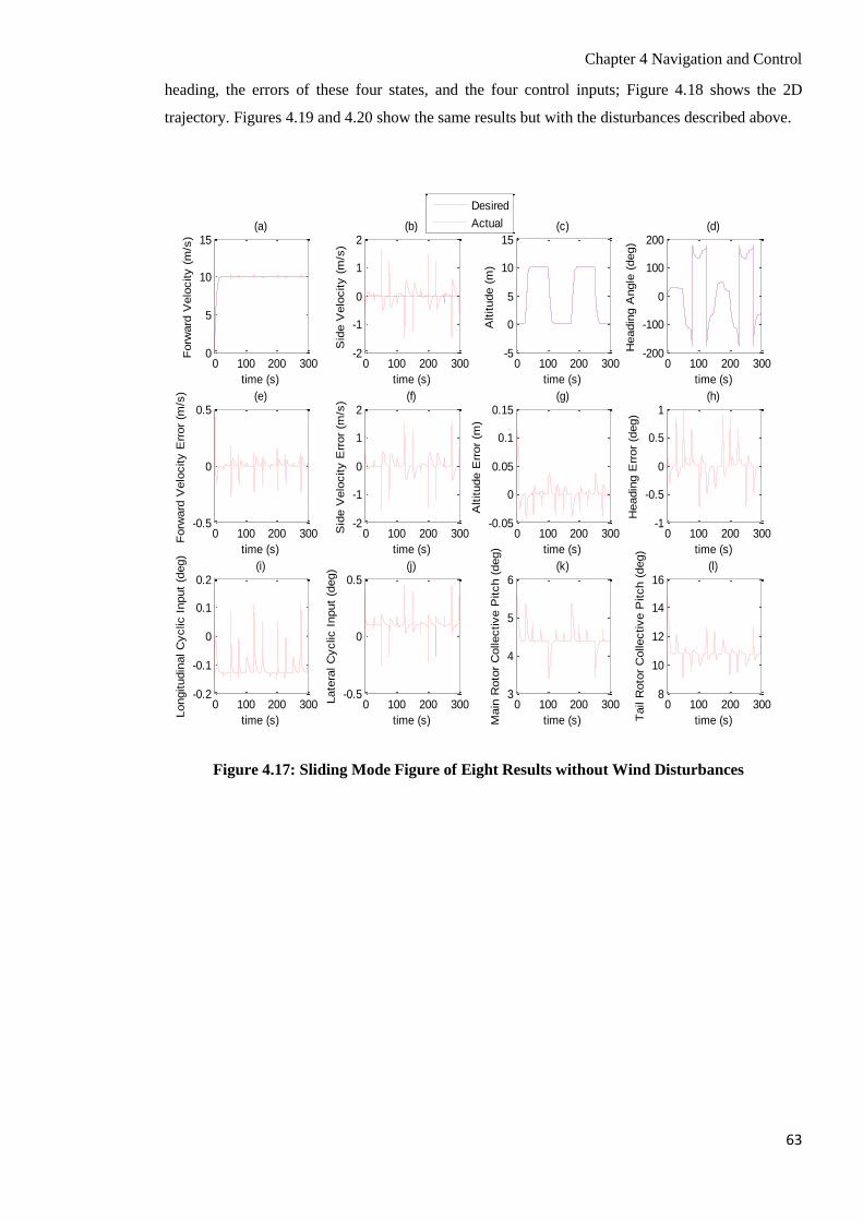
Chapter 4 Navigation and Control
63
heading, the errors of these four states, and the four control inputs; Figure 4.18 shows the 2D
trajectory. Figures 4.19 and 4.20 show the same results but with the disturbances described above.
Figure 4.17: Sliding Mode Figure of Eight Results without Wind Disturbances
0 100 200 3000
5
10
15
time (s)
Forw
ard
Velo
city (
m/s
)
(a)
Desired
Actual
0 100 200 300-2
-1
0
1
2
time (s)
Sid
e V
elo
city (
m/s
)
(b)
0 100 200 300-5
0
5
10
15
time (s)
Altitude (
m)
(c)
0 100 200 300-200
-100
0
100
200(d)
time (s)
Headin
g A
ngle
(deg)
0 100 200 300-0.5
0
0.5
time (s)
Forw
ard
Velo
city E
rror
(m/s
) (e)
0 100 200 300-2
-1
0
1
2
time (s)
Sid
e V
elo
city E
rror
(m/s
) (f)
0 100 200 300-0.05
0
0.05
0.1
0.15
time (s)
Altitude E
rror
(m)
(g)
0 100 200 300-1
-0.5
0
0.5
1
time (s)
Headin
g E
rror
(deg)
(h)
0 100 200 300-0.2
-0.1
0
0.1
0.2
time (s)
Longitudin
al C
yclic I
nput
(deg)
(i)
0 100 200 300-0.5
0
0.5
time (s)
Late
ral C
yclic I
nput
(deg) (j)
0 100 200 3003
4
5
6
time (s)Main
Roto
r C
ollective P
itch (
deg)
(k)
0 100 200 3008
10
12
14
16
time (s)Tail R
oto
r C
ollective P
itch (
deg)
(l)

Chapter 4 Navigation and Control
64
Figure 4.18: Sliding Mode 2D Trajectory without Wind Disturbances
Figure 4.19: Sliding Mode Figure of Eight Results with Wind Disturbances
-50 0 50 100 150 200 250-100
0
100
200
300
400
500
East Position [m]
Nort
h P
ositio
n [
m]
0 100 200 300-5
0
5
10
15
time (s)
Forw
ard
Velo
city (
m/s
)
(a)
Desired
Actual
0 100 200 300-2
-1
0
1
2
time (s)
Sid
e V
elo
city (
m/s
)
(b)
0 100 200 300-5
0
5
10
15
time (s)
Altitude (
m)
(c)
0 100 200 300-200
-100
0
100
200(d)
time (s)
Headin
g A
ngle
(deg)
0 100 200 300-1
-0.5
0
0.5
1
time (s)
Forw
ard
Velo
city E
rror
(m/s
) (e)
0 100 200 300-2
-1
0
1
2
time (s)
Sid
e V
elo
city E
rror
(m/s
)
(f)
0 100 200 300-0.2
-0.1
0
0.1
0.2
time (s)
Altitude E
rror
(m)
(g)
0 100 200 300-4
-2
0
2
4
time (s)
Headin
g E
rror
(deg)
(h)
0 100 200 300-0.4
-0.2
0
0.2
0.4
time (s)
Longitudin
al C
yclic
Input
(deg) (i)
0 100 200 300-0.5
0
0.5
time (s)
Late
ral C
yclic
Input
(deg)
(j)
0 100 200 3002
4
6
8
time (s)Main
Roto
r C
olle
ctive P
itch (
deg)
(k)
0 100 200 3000
5
10
15
20
time (s)
Tail
Roto
r C
olle
ctive P
itch (
deg)
(l)
Start

Chapter 4 Navigation and Control
65
Figure 4.20: Sliding Mode 2D Trajectory with Wind Disturbances
Like the PID controller, the Sliding Mode controller performs well with and without the wind
disturbances, with the state errors being relatively small, and the helicopter tracing out a figure-of-
eight pattern. Also, the state errors increase when the disturbances are introduced, with the most
significant changes being observed in the heading and altitude. In this case, the 2D trajectory does
not appear to be affected by the wind disturbances, unlike the PID controller.
4.9 Comparison of PID and Sliding Mode Controllers
The PID and Sliding Mode controllers are now compared by examining the average errors in each
state during the commanded changes in each of the four states. Table (4.4) shows the average state
errors in the simulation that involves changes in the surge command, Table (4.5) shows the average
state errors in the simulation that involves changes in the sway command, Table (4.6) shows the
average state errors in the simulation that involves changes in the altitude command, and Table
(4.7) shows the average state errors in the simulation that involves changes in the heading
command. The average state errors are calculated by measuring the error at each time step and
finding the average of all these values; effectively, each state error is integrated over the entire
simulation and then divided by the simulation time to obtain the average.
-50 0 50 100 150 200 250-100
0
100
200
300
400
500
East Position [m]
Nort
h P
ositio
n [
m]
Start

Chapter 4 Navigation and Control
66
Table 4.4: Average State Errors – Surge Changes
Surge Error
(m/s)
Sway Error
(m/s)
Altitude Error
(m)
Heading Error
(rad)
PID 0.0803 0.0476 0.0151 0.0135
Sliding Mode 0.1488 0.0291 0.0359 0.0028
Table 4.5: Average State Errors – Sway Changes
Surge Error
(m/s)
Sway Error
(m/s)
Altitude Error
(m)
Heading Error
(rad)
PID 0.0062 0.2036 0.0037 0.0059
Sliding Mode 0.0007 0.0960 0.0090 0.0003
Table 4.6: Average State Errors – Altitude Changes
Surge Error
(m/s)
Sway Error
(m/s)
Altitude Error
(m)
Heading Error
(rad)
PID 0.0012 0.0127 0.0080 0.0044
Sliding Mode 0.0001 0.0075 0.0074 0.0015
Table 4.7: Average State Errors – Heading Changes
Surge Error
(m/s)
Sway Error
(m/s)
Altitude Error
(m)
Heading Error
(rad)
PID 0.0661 0.3022 0.0047 0.0089
Sliding Mode 0.0225 0.2371 0.0038 0.0009
From these results, it can be seen that the average heading and side velocity (sway) errors are less
for the Sliding Mode controller in all four simulations. In fact, the average heading error is
significantly lower for the Sliding Mode controller in all four simulations. The average altitude
error is larger for the Sliding Mode controller during the surge and sway changes, but is lower
during the altitude and heading changes, although not by much. The average forward velocity
(surge) error is larger for the Sliding Mode controller during the surge changes (which was also
observed when comparing Figures 4.10 and 4.16), but smaller for the other three simulations. In
general, the PID controller performs slightly better than the Sliding Mode controller when
controlling the altitude, but the Sliding Mode controller performs better in the other cases. It has
also been observed when comparing Figures 4.10 and 4.16 that the errors are corrected more
quickly and efficiently for the Sliding Mode controller.
The PID and Sliding Mode controllers are also compared for the figure-of-eight trajectory.
Comparing Figures 4.11 and 4.17, it can be seen that when there are no disturbances, the errors are
corrected more quickly and efficiently with the Sliding Mode controller, and also the actuator

Chapter 4 Navigation and Control
67
responses are more efficient, in the sense that they are less oscillatory in nature. When there are
disturbances, comparing Figures 4.13 and 4.19, there does not appear to be too much difference in
the nature of the response, although it is noticeable that the heading error is smaller with the Sliding
Mode controller. The actuator responses are similar in this case, with the random disturbances
causing more oscillations in both controllers. The wind disturbances seem to have less of an effect
on the 2D trajectory of the helicopter with the Sliding Mode controller than with the PID controller.
Numerical values of the state errors are compared for each controller with and without the wind
disturbances. Tables 4.8 and 4.9 show the average error of each state for the different controllers in
each scenario.
Table 4.8: Average State Errors without Disturbances – Figure of Eight
Surge Error
(m/s)
Sway Error
(m/s)
Altitude Error
(m)
Heading Error
(rad)
PID 0.0804 0.2544 0.0088 0.0098
Sliding Mode 0.0319 0.1936 0.0071 0.0019
Table 4.9: Average State Errors with Disturbances – Figure of Eight
Surge Error
(m/s)
Sway Error
(m/s)
Altitude Error
(m)
Heading Error
(rad)
PID 0.0948 0.2810 0.0183 0.0259
Sliding Mode 0.0848 0.2271 0.0258 0.0123
Even though the disturbances have had more of an effect on the Sliding Mode controller than the
PID controller, the average state errors are always smaller for the Sliding Mode controller except
for the altitude when there are disturbances. In particular, the heading error is significantly smaller
for the Sliding Mode controller. After running several simulations, it was found that in order to
achieve this level of performance (particularly without disturbances) with the PID controller, the
gains must be increased to the point that the stability of the system is threatened.
Overall, the Sliding Mode controller performs better than the PID controller, so the Sliding Mode
controller is used for the helicopter in future simulations. In terms of implementation, it was found
in Gavrilets (2003) that a single execution of estimation and control logic (LQR controller) took
less than 2ms, which is well within the time required to update the actuators. It was also found that
simulations on Matlab ran between six and seven times faster than real time. Therefore, it is
expected that implementation of the Sliding Mode controller would not cause any real problems.

Chapter 4 Navigation and Control
68
4.10 Summary
This chapter introduced the navigation and control systems that are used for the simulations. The
overall control strategy for the helicopter was discussed, as was the theory behind the two
controllers used: PID and Sliding Mode. The strategy used for collision avoidance was also
discussed.
The navigation system of the helicopter during forward flight was introduced, and is based on a
line-of-sight autopilot, which calculates a desired heading angle based on the desired position of
the vehicle in the xy-plane. The desired heading is generated so that the vehicle points towards the
desired point, so that as the vehicle moves forward, it travels towards that point.
The collision avoidance strategy was discussed, and is based on the concept of a collision cone.
The collision cone calculates a set of directions for the velocity vector that will result in a collision
at some point if all other states remain the same.
The theory of PID and Sliding Mode control were presented, as well as the ways in which they are
applied to the particular system being studied in this thesis. Results were shown for both controllers
to indicate how the helicopter can be controlled, and the results for both controllers were compared.
It was found that the Sliding Mode controller gave a better overall response, correcting errors more
quickly and more efficiently.
In summary, this chapter describes how the vehicles are navigated and controlled, so that they can
visit desired points, thus carrying out an appropriate search mission.

Chapter 5 Search Algorithms and Implementation
69
Chapter 5
Search Algorithms
5.1 Introduction
The work presented in this thesis is a study of the effectiveness of search algorithms in the context
of an autonomous system performing an air-sea search mission. There are many optimisation
problems that cannot be solved exactly using calculus or an exhaustive search. A good example of
this is the Travelling Salesman Problem [Johnson & Picton, 1995], where a salesman must visit a
group of cities (all exactly once) and return to the origin city such that the total distance travelled is
minimised. Given that the cities are in discrete locations, the problem cannot be solved using basic
calculus, and given that the number of possible paths increases astronomically as the number of
cities increases [Johnson & Picton, 1995], an exhaustive search is impractical except for a small
number of cities. In this thesis, a search is being carried out of an area of the sea containing
survivors of a sinking ship. The search area is too large to search exhaustively, so this type of
problem cannot be solved using basic methods. This is where more advanced search algorithms
come into play; in this context, the search algorithms can be used to generate points to be visited,
and the agents are instructed to search those points and evaluate the solutions. Once the search
algorithm generates a point, the navigation system generates appropriate outputs, and the controller
then drives the system towards these outputs, so that the vehicle can reach the desired position.
This entire system is illustrated in block diagram form in Figure 5.1.
Figure 5.1: Overall System
Navigation
System
Collision
Avoidance
Control
System
System
Dynamics
Outputs
Desired
Position
Position
Modified
Desired
Outputs
Desired
Inputs
Desired
Outputs
Velocity, Altitude
& Heading
Velocity, Altitude
& Heading
Search
Algorithm
Position

Chapter 5 Search Algorithms and Implementation
70
Several different types of search algorithms are introduced in this chapter. Different approaches are
used in each algorithm, such as searching randomly, cooperatively, in a structured manner, and by
following specific patterns. Some algorithms even use combinations of these approaches. Three
search algorithms, which are actually used in manned search and rescue, are tested on the
autonomous system, and are used as benchmarks for comparison with the optimisation techniques
applied. These three algorithms are known as Parallel Sweep, Sector Search, and Expanding
Square [IAMSAR, 2008], and are examples of search algorithms that follow a specific structure.
Other search algorithms use a more random approach, such as the Random Search [Johnson &
Picton, 1995]. Some algorithms use knowledge gained throughout the search as a factor in the
remainder of the search; these algorithms come under the category of heuristics [Rayward-Smith et
al 1996]. The heuristic methods used in this thesis are Hill Climbing [Johnson & Picton, 1995;
Russell & Norvig, 1995], Simulated Annealing [Johnson & Picton, 1995; Kirkpatrick et al, 1983],
Ant Colony Optimisation [Dorigo & Di Caro, 1999; Dorigo et al, 2006], Genetic Algorithms
[Holland, 1992; Mitchell, 1995], and Particle Swarm Optimisation [Eberhart & Kennedy, 1995;
Kennedy & Eberhart, 1995]. The latter three algorithms are examples of cooperative search
algorithms, where the multiple vehicles involved in the search exchange information, which
influences the remainder of the search for each vehicle. As well as these heuristic methods, a
heuristic version of the Random Search is also tested by means of a weighted probability
distribution (see Chapter 7).
Search algorithms use a cost or evaluation function to quantify and assess the performance of each
candidate solution it has generated. In this case, the aim is to search for survivors of a sinking ship
at sea, so temperature would be a good measure of a human being detected by sensors on board the
search vehicles. Search algorithms must also have a terminating condition, which tells the
algorithm to stop searching. Such a condition might be when an acceptable solution has been found,
when so many solutions have been checked, or when a certain length of time has passed. In this
case, because of the time constraints imposed by the fuel consumption of the vehicle and its limited
payload, the terminating condition is set so that the algorithms stop after a fixed length of time.
Section 5.2 of this chapter discusses some of the standard manned search procedures carried out in
real-life rescue operations; these algorithms are used in the context of the autonomous system for
comparison. Section 5.3 then discusses the theory and mechanism associated with the optimisation
techniques considered in this study. Section 5.4 summarises this chapter.
5.2 Standard Search Patterns
This section describes three common search procedures used in real search and rescue operations.
Although these procedures are used for manned searches [IAMSAR, 2008] they are applied to the

Chapter 5 Search Algorithms and Implementation
71
autonomous system so that they can be used as a benchmark for the more advanced optimisation
techniques.
5.2.1 Parallel Sweep
The Parallel Sweep [IAMSAR, 2008] (or parallel track) search pattern involves a vehicle searching
within a rectangular search area. The search starts just inside the corner of the rectangle;
specifically, the distance from the starting point to each edge is equal to half the track space
[IAMSAR, 2008]. The search is then carried out by performing parallel sweeps, with the main
tracks being parallel to the longer side of the rectangle [IAMSAR, 2008].This is illustrated in
Figure 5.2.
Figure 5.2: Parallel Sweep Path
This method is often used when there is large uncertainty in the target locations, so that a large area
can be searched with uniform coverage [IAMSAR, 2008].
5.2.2 Sector Search
The Sector Search [IAMSAR, 2008] scans sectors of a circle centred at some datum point. The
search pattern is illustrated in Figure 5.3. The search starts at the centre of the circle, and travels
along a radius to the circumference, then turns 120° in the starboard direction (clockwise when
looking from above). This pattern is repeated i.e. travels forward and then turns 120° in the
Start
Track Space, S
S/2
S/2

Chapter 5 Search Algorithms and Implementation
72
starboard direction every time it reaches the circumference. Ultimately the path traces out three
equilateral triangles, whose lengths are equal to the radius of the circle.
Figure 5.3: Sector Search Path
If there is enough time, a second search can be carried out using the same pattern but rotated 30°
from the first search, so that the search legs for the second search are halfway between those for the
first search [IAMSAR, 2008]. This is illustrated in Figure 5.4, with the dashed lines representing
the second search.
Figure 5.4: Extended Sector Search Path
Start
120°
Start
120°
First Leg of
Second Search

Chapter 5 Search Algorithms and Implementation
73
The Sector Search method is used when the target locations are known with reasonable accuracy,
and covers a lot of ground near the centre of the search [IAMSAR, 2008].
5.2.3 Expanding Square
The Expanding Square [IAMSAR, 2008] method starts at a central point, like the Sector Search,
and then travels along sides of squares, with the square increasing in length every two steps. This is
made clearer in Figure 5.5.
Figure 5.5: Expanding Square Path
The search proceeds by moving forward 1 unit (where a unit is equal to the track space), turning
90° clockwise, moving forward 1 unit, turning 90° clockwise, moving forward 2 units, turning 90°
clockwise, moving forward 2 units, turning 90° clockwise, moving forward 3 units, and so on. In
short, the vehicle moves a given number of units twice, and then increases the distance by 1, and
the vehicle also turns 90° clockwise between each movement, thus tracing out a square of
expanding length. A second search can be carried out if necessary, with the second square being at
a 45° angle relative to the first square, as illustrated in Figure 5.6, with the second path being
represented by the dashed line.
1
2
2 1
3
3
4
4
5
5
6
6
7
7
8
8
9
Start
Track Space

Chapter 5 Search Algorithms and Implementation
74
Figure 5.6: Extended Expanding Square Path
Like the Sector Search, the Expanding Square search method is often used if the target locations
are known with reasonable accuracy [IAMSAR, 2008].
5.3 Optimisation Techniques
This section introduces several common search/optimisation algorithms, which are applied to the
simulations in this thesis. These methods are used because searching for survivors in the sea can be
considered an optimisation problem, with the optima being the locations of survivors. Also, unlike
the standard search patterns discussed in Section 5.2, most of these optimisation techniques use
information gained throughout the search as factors in where the rest of the search takes place,
rather than simply following a set pattern.
Start
First Leg of
Second Search

Chapter 5 Search Algorithms and Implementation
75
5.3.1 Random Search
The Random Search [Johnson & Picton, 1995], as the name suggests, simply picks out a random
solution at each iteration and evaluates it. The algorithm continues in this way without using any
information gained during the search. Typically, random solutions can be generated using random
number generators in Matlab, such as the rand and randi functions. Because of the obvious random
nature of this algorithm, many different areas of the search space are often covered, but no
knowledge is used from previous points in the search to determine the next point, so even if a good
solution is found, this does not influence the remainder of the search. It is therefore possible that
even if a large part of the search space is covered, a good solution may not be found, as there is no
guarantee that the basic Random Search will search the best areas.
5.3.2 Hill Climbing
The Hill Climbing algorithm [Johnson & Picton, 1995] is a search method that uses knowledge
gained from other points that have already been visited. The algorithm starts with an initial solution,
and then performs a local search. At each iteration a ‘nearby’ solution is evaluated and compared to
the current solution: if the local solution is better than the current solution, then the current solution
is updated to this local solution; if the local solution is not any better than the current solution, then
the current solution remains as it is. The process then continues in this way until a termination
condition is met.
Hill Climbing is an example of a local-search algorithm [Rayward-Smith et al 1996], as it only
searches in the immediate vicinity of the current solution. In the context of searching a region (as is
the case here), “immediate vicinity” does have an obvious meaning, but for a general problem, one
must consider how to define the immediate vicinity of a solution. Generally, the immediate vicinity
(or neighbourhood) refers to a set of solutions that can be obtained from the original solution
without changing many of its characteristics.
The main advantages of Hill Climbing are that it is very simple and so does not require a great deal
of computational power, and it does not require a lot of memory, so it is very easy to run this
algorithm on a computer; it could even be done by hand, depending on how many iterations are
required.
Since Hill Climbing is a local-search algorithm, it is unlikely to search a large region of the search
space. Indeed, it is possible that the algorithm will become stuck: if, for example, the algorithm
encounters a local minimum or maximum, or a plateau [Russell & Norvig, 1995], then it is unable
to proceed any further. A local minimum/maximum is a point where the function being evaluated is
at its minimum/maximum with respect to the neighbourhood of that point, but it is not necessarily

Chapter 5 Search Algorithms and Implementation
76
the global minimum/maximum. A plateau is a region where all the solutions give the same value of
the function being evaluated, so the algorithm is unable to proceed as the surrounding solutions are
not any better than the current solution. One way to overcome such problems is to include the
condition that if there is no improvement after a certain number of iterations, then the algorithm
restarts from a random solution, while still saving the best solution. Thus, the algorithm is more
likely to search a larger region of the search space.
5.3.3 Simulated Annealing
Simulated Annealing [Johnson & Picton, 1995; Kirkpatrick et al, 1983; McGookin, 1997;
McGookin & Murray-Smith, 2006; Kirkpatrick, 1984; Russell & Norvig, 1995] is an optimisation
technique that is very similar to Hill Climbing. Like Hill Climbing, Simulated Annealing involves a
local search around a “current” candidate solution. The main difference between the two is the
criteria for selecting new solutions. As explained, Hill Climbing only accepts a new solution if it is
better than the current solution; Simulated Annealing includes the possibility of accepting poorer
solutions, meaning that the algorithm can escape from local minima/maxima. Simulated Annealing
is based on the physical process of annealing: a process that involves heating a metal until it is
molten and then allowing it to cool by regulating the temperature [McGookin, 1997] until the
ground state is reached.
The physical process of annealing – which finds ground states of matter – provides the inspiration
for finding the best solutions to combinatorial problems using Simulated Annealing: the value of
the target function plays the role of the energy of the physical state, and the best solution represents
the ground state of the physical system. The local search part of Simulated Annealing is analogous
to the perturbations in the states of the physical system.
Metropolis et al (1953) devised a way of simulating the process of annealing, where the system is
perturbed, and the change in energy, ΔE, from the initial state to the perturbed state is determined.
If ΔE < 0 (so that the perturbed state has lower energy than the initial state), then the perturbed
state is accepted; otherwise, the perturbed state is accepted with probability P(ΔE) = exp(–ΔE/kBT),
where kB is Boltzmann’s constant and T is the temperature of the system. Based on this probability,
it can be seen that higher energy states are likely to be accepted if the increase in energy is small
and/or the temperature is high. This algorithm for determining whether or not a new solution
should be accepted is known as the Metropolis Procedure, or Metropolis Criterion [Kirkpatrick et
al, 1983, Worrall, 2008].
The Metropolis Procedure, as described above can be implemented on Matlab using random
numbers. The temperature, T, can be thought of as a control parameter: at first, when the system
has been “melted”, the temperature is high, and the perturbations are large; as more iterations are

Chapter 5 Search Algorithms and Implementation
77
performed, this effective temperature is decreased according to some annealing schedule
[Kirkpatrick et al, 1983; Sharman, 1988; Worrall, 2008], and the perturbations become smaller
[McGookin, 1997]. Typically, the temperature is decreased from T to αT for some constant α
between 0 and 1, so after n iterations, the effective temperature is
T = αnT0 (5.1)
where T0 is the initial temperature. As more iterations are performed, the temperature converges to
zero and, according to the Metropolis Criterion, the acceptance of poorer solutions becomes very
unlikely, and the Simulated Annealing Algorithm effectively becomes a Hill Climbing Algorithm.
Like Hill Climbing, it is also convenient to allow the option of a random restart with Simulated
Annealing if no new solutions are accepted after a given number of iterations. The Simulated
Annealing algorithm could still get stuck at local optima, so allowing the random restart can further
diversify the search.
5.3.4 Genetic Algorithms
A Genetic Algorithm [Goldberg, 1989; Holland, 1992; Johnson & Picton, 1995; Krcmar & Dhawan,
1994; Mitchell, 1995; Alfaro-Cid, 2003; Schmitt, 2004] is an optimisation technique that mimics
the biological process of natural selection and evolution. This technique can be attributed to John
Holland, who started the development of the theory in the 1960s, before describing the theory in
Holland (1975). A Genetic Algorithm can be thought of as a mathematical evolution of a
population of solutions: in nature, organisms evolve by means of natural selection and reproduction,
along with occasional modifications by mutation [Holland, 1992]. Only the fittest organisms
survive as long as the reproduction step, where genes are mixed and recombined to form a new
generation. Over a large number of generations, only the best organisms survive. A Genetic
Algorithm mimics this process by representing solutions as “chromosomes” whose fitness can be
evaluated via a “fitness function”, which is equivalent to the target function for the particular
problem. The appropriate chromosomes are then selected as parents for the reproduction stage; this
process is known as selection [Dirk & Goldberg, 1994]. During the reproduction stage, the genes
are mixed and recombined to form “offspring”; this process is known as crossover [Khoo &
Suganthan, 2002]. Certain genes in the offspring chromosomes are then mutated probabilistically;
this process is known as mutation [Holland, 1975; Khoo & Suganthan, 2002; McGookin, 1997].
The new population is then evaluated, and the process repeats over and over again, with the aim of
finding the best solution to the problem, corresponding to the “fittest” chromosome.

Chapter 5 Search Algorithms and Implementation
78
5.3.4.1 Encoding and Decoding
The first step in applying a Genetic Algorithm to a problem is determining how to encode the
solutions so that they can be represented in chromosome form. Of course, this depends on the
individual problem, but one very common way to encode solutions is to write them as strings of ‘1s’
and ‘0s’. For example, if solutions can be represented by simple numbers, then they can be
converted to binary, and can therefore be written as strings of ‘1s’ and ‘0s’. For some problems,
working out how to encode solutions can be rather tricky, such as for the Prisoner’s Dilemma
[Axelrod, 1987; Goldbeck, 2002; Mitchell, 1995]. The basic form of this problem/game is that two
people are arrested for committing a crime, and are placed in separate rooms to be interrogated,
without any communication between them. If both people testify against each other, then they each
receive a 4 year sentence; if one person testifies and the other doesn’t, then the person who testifies
receives a suspended sentence with probation, and the other person receives a 5 year sentence; if
neither testify, then they each receive a 2 year sentence. Whatever the other person does, the best
option either way is to testify against them, but the dilemma is that the result is better if neither
testify than if both testify. This can be reinterpreted as the following game between 2 people: if
both players cooperate, they each get 3 points; if one player cooperates and the other player defects,
then the player who defects receives 5 points and the player who cooperates receives 0 points; if
both players defect then they each receive 1 point. Mitchell (1995) describes how to encode
different strategies: each strategy is based on the 3 previous turns, of which there are 64
possibilities (2 choices for each person and 3 shots each), so there are 264
possible strategies (2
choices for each of the 64 combinations of previous turns). The first shot for each player is
determined by 3 hypothetical previous turns, of which there are 26 possibilities, so overall, there are
270
strategies, with each strategy being encoded by a 70-bit string. If “cooperate” is represented by
the digit 1, and “defect” is represented by the digit 0, each strategy can be encoded as a
chromosome consisting of 70 digits, each being either 0 or 1.
In the problem being considered in this thesis, the solutions are simply 2-dimensional coordinates,
and instead of converting them to binary, the real number representation (up to one decimal place
in this case) is used, as in McGookin (1997) and Worrall (2008). The region being considered in
the xy-plane is the square with x and y values ranging from –200 to +200. If the coordinates are
written to one decimal place, then each of the x and y coordinates can be defined by five
characters: the sign (plus or minus, with ‘1’ representing plus and ‘0’ representing minus), the
hundreds digit (0 or 1), the tens digit (ranging from 0 to 9), the unit digit (ranging from 0 to 9), and
the digit after the decimal point (ranging from 0 to 9). Thus a coordinate of the form (x,y) in this
region can be represented by an 10-bit string. For example, the point (124.3, –78.6) can be written
in the chromosome form shown in Figure 5.7, and decoded.

Chapter 5 Search Algorithms and Implementation
79
1 1 2 4 3 0 0 7 8 6
Figure 5.7: Encoding and Decoding
5.3.4.2 Selection
The next step in developing a Genetic Algorithm is deciding on the method used for selection. This
involves determining the fitness of the solutions using the appropriate fitness function. The three
most common selection methods are Elitist, Roulette Wheel, and Tournament Selection. The Elitist
method [Dwivedi et al, 2012; McGookin et al, 1997] keeps the best solutions from one generation
to the next. The fraction of the population that is kept from one generation to the next can be
specified by the designer; the top 20% of the population for example, may be stored for the next
generation, and the rest of the population is chosen randomly. This method has the advantage that
the best solutions are not lost between generations, but has the disadvantage that it sometimes has a
tendency to converge too quickly [McGookin et al, 1997]. To avoid this, a higher mutation rate is
required.
The Roulette Wheel method [Goldberg, 1989; Rayward-Smith et al, 1996] works by selecting
parent chromosomes with weighted probabilities based on their relative fitness. In this sense,
selecting a parent is like spinning a Roulette Wheel with slots whose sizes are directly proportional
to the fitness of the corresponding chromosomes. Therefore, statistically, the good solutions are
more likely to be selected than the poor solutions. This selection method preserves a certain amount
of randomness, which is often essential in covering a reasonable amount of the search space.
Tournament Selection involves holding “tournaments”, where a fixed number of chromosomes
from the population are randomly selected, and their fitness values are compared. Once enough
tournaments have been held, the winners (best solutions) are selected for the crossover stage
[Miller & Goldberg, 1995; Rayward-Smith et al, 1996]. Again, this allows a certain amount of
randomness in the selection process and reduces the need for a higher mutation rate.
+ 1
(×102)
2
(×101)
4
(×100)
3
(×10–1
) – 0
(×102)
7
(×101)
8
(×100)
6
(×10–1
)
(124.3, –78.6)
x-coordinate y-coordinate

Chapter 5 Search Algorithms and Implementation
80
5.3.4.3 Crossover
The next step in the Genetic Algorithm is the crossover process, where the selected parent
chromosomes recombine to form new offspring chromosomes. This is done by selecting two parent
chromosomes and exchanging sequences from each chromosome to form the child chromosomes,
which, as a result of the exchange process, have characteristics of each of the two parent
chromosomes. For example, consider a pair of parent chromosomes, which are written as 16-bit
strings of 0s and 1s. i.e. 1101000101101110 and 0100011010110101. These can be combined by
selecting a random crossover point, and then swapping the sequences after that point in each
chromosome. For example, suppose the crossover point is after the ninth digit in each chromosome,
as illustrated in Figure 5.8.
1 1 0 1 0 0 0 1 0 1 1 0 1 1 1 0
0 1 0 0 0 1 1 0 1 0 1 1 0 1 0 1
1 1 0 1 0 0 0 1 0 0 1 1 0 1 0 1
0 1 0 0 0 1 1 0 1 1 1 0 1 1 1 0
Figure 5.8: Crossover
The “1101110” from the first chromosome swaps with the “0110101” from the second
chromosome, resulting in the offspring chromosomes as shown. Hence, the offspring chromosomes
from this crossover are 1101000100110101 and 0100011011101110.
The particular crossover technique illustrated above is an example of single-point crossover [Khoo
& Suganthan, 2002], which means that exactly one crossover point is selected, and the two
chromosomes are swapped from that point onwards. It is also possible to select more than one
crossover point and swap the chromosomes in regions between these crossover points, such as in
two-point crossover [Khoo & Suganthan, 2002; Worrall, 2008]. With two-point crossover, two
crossover points are selected and the chromosomes are swapped in between those two points. In the
above example, if the crossover points are after the fifth and twelfth digits in each chromosome,
then digits six to twelve will swap to form the child chromosomes. This crossover process is
illustrated in Figure 5.9.
Parents
Offspring

Chapter 5 Search Algorithms and Implementation
81
1 1 0 1 0 0 0 1 0 1 1 0 1 1 1 0
0 1 0 0 0 1 1 0 1 0 1 1 0 1 0 1
1 1 0 1 0 1 1 0 1 0 1 1 1 1 1 0
0 1 0 0 0 0 0 1 0 1 1 0 0 1 0 1
Figure 5.9: Two-point Crossover
The “0010110” from the first chromosome swaps with the “1101011” from the second
chromosomes, resulting in the offspring chromosomes as shown. Hence, the offspring
chromosomes from this crossover are 1101011010111110 and 0100000101100101. There are other
types of crossover methods, like uniform crossover [Khoo & Suganthan, 2002], gene-lottery
[Schmitt, 2004] and those used for problems like the Travelling Salesman Problem [Bryant &
Benjamin, 2000; Dwivedi et al, 2012; Homaifar et al, 1992; Wei & Lee, 2004]; the type of
crossover method that should be used depends on the problem and how the solutions are encoded.
In this thesis, single-point crossover is used.
5.3.4.4 Mutation
The final step in Genetic Algorithms is mutation, which involves slight probabilistic changes in the
child chromosomes formed during the crossover stage [Holland, 1975; Khoo & Suganthan, 2002;
McGookin, 1997]; when a child chromosome is formed, some of the genes may be randomly
flipped, as is the case with real chromosomes. The number of genes that are flipped in each child
chromosome depends on the mutation rate, which can be specified by the designer. Mutation can
be implemented by randomly altering each gene with a probability given by this mutation rate. As
an example, consider the child chromosomes given in Figure 5.9, which are 1101011010111110
and 0100000101100101. If the first chromosome flips the fourth and eleventh genes, and the
second chromosome flips the third gene, then the resulting mutated child chromosomes are
1100011010011110 and 0110000101100101. The choice of mutation rate can have a significant
impact on the performance of the algorithm: as mentioned in Chapter 2, a high mutation rate
encourages a high level of exploration of the search space, but possibly at the expense of
Parents
Offspring

Chapter 5 Search Algorithms and Implementation
82
continually jumping away from good solutions; a low mutation rate keeps the Genetic Algorithm
structure, but may lead to a more local search, meaning that the algorithm could get stuck.
Based on the discussions on different methods for encoding, selection, crossover and mutation, it is
clear that there are a vast number of forms of Genetic Algorithms that can be implemented for a
single problem. For practical reasons, not all of these variations can be tested, so the different parts
of the Genetic Algorithm should be chosen sensibly. Understanding why Genetic Algorithms work
involves investigating the notion of schemas [Mitchell, 1995], which are basically the building
blocks of the solutions [Mitchell, 1995]. In this context good solutions exhibit similar patterns of
allele values and thus have common schema. It can be shown that statistically, the number of good
schemas is likely to increase, and the bad schemas are likely to be destroyed.
5.3.5 Particle Swarm Optimisation
Particle Swarm Optimisation [Eberhart & Kennedy, 1995; Eberhart & Shi, 2001; Kennedy &
Eberhart, 1995], as discussed in Chapter 2, is an optimisation technique that finds solutions by
effectively “flying” through the search space. The method was first developed by Kennedy and
Eberhart in 1995 after several scientists attempted to simulate the choreography of bird flocking
[Eberhart & Shi, 2001]. The flocking of birds is very fascinating in the sense that it is extremely
unpredictable, yet incredibly elegant: they can change direction and scatter very quickly, yet they
can still regroup and flock in a very synchronous fashion.
The first simulation involved nearest-neighbour velocity matching [Kennedy & Eberhart, 1995],
where each bird or agent determined its nearest neighbour and changed its velocity vector to match
that of the nearest neighbour. This resulted in the flock quickly finding a unanimous, unchanging
direction, so a random variable called craziness was introduced to the system [Kennedy & Eberhart,
1995]. After this, came the introduction of the cornfield vector [Kennedy & Eberhart, 1995]: a
vector that attempts to drive each agent towards its own best solution and the best solution of the
whole flock. Each agent had knowledge of its best solution so far, and the best solution obtained by
the entire flock so far. The velocity components were then adjusted by random increments in the
appropriate directions. This proved to be successful, and it was also found that the craziness and
nearest neighbour terms were unnecessary when the cornfield vector was included. From this point,
it was natural to extend the simulations to multidimensional searches, and the Particle Swarm
Optimisation algorithm emerged, as described below.
Consider a problem space with D dimensions, and let there be N agents or “particles” searching for
solutions. The current solution or “position” has ND elements: D components for each of the N
agents. Denote the dth component of the position of the i
th particle by xid. Similarly, each particle is
given a “velocity” vector: the dth component of the velocity of the i
th particle is denoted vid. The d
th

Chapter 5 Search Algorithms and Implementation
83
component of the “best” position of the ith particle is denoted pid and the d
th component of the best
position of all N particle is denoted pgd, where the “g” represents “global”. At each iteration, the
position and velocity of each particle are updated according to Equations (5.2) and (5.3):
idgd2idid1idid xprandcxprandcvv (5.2)
ididid vxx (5.3)
Here c1 and c2 are acceleration constants, and rand represents a random number between 0 and 1,
with the two random numbers in Equation (5.2) being generated independently. As well as
updating position and velocity, the “particle” and “global” best solutions are also updated at each
iteration. Thus there is a random movement of each particle towards its own best solution and the
best solution of the whole group. The terms that are added on to the velocity are a modification of
the cornfield vector, as the cornfield vector did not take into account the “distances” from the
present solution to the particle best and global best solutions, whereas this version results in an
acceleration by distance [Kennedy & Eberhart, 1995], due to the (pid – xid) and (pgd – xid) terms.
Originally, it was found that the algorithm seemed to perform best when the constants c1 and c2
were both set equal to 2.0 [Eberhart & Shi, 2001]. A limit must also be set on the maximum
velocity of the particle.
Over the years, some modifications have been made, such as the inclusion of an inertia weight
[Eberhart & Shi, 2000; Eberhart & Shi, 2001] and a constriction factor [Clerc & Kennedy, 2002;
Eberhart & Shi, 2000]. The constriction factor, represented by “K”, can be included in Equation
(5.2), so that the modified velocity update equation is now
idgd2idid1idid xprandcxprandcvKv (5.4)
The constriction factor K is given by
4φφφ2
2K
2
(5.5)
where φ = c1 + c2, and φ > 4. According to Eberhart & Shi (2001), c1 and c2 are typically both set to
2.05, so that φ = 4.1 and hence, K = 0.730. Also, it was found that a reasonable limit for the
maximum velocity of each particle is the dynamic range of each particle on each dimension
[Eberhart & Shi, 2000; Eberhart & Shi, 2001].
In many optimisation problems, the variables are constrained in some way; the task is often to
minimise/maximise a certain function under a set of constraints. This can be problematic when
updating the velocity and position of each particle, as the update equations do not take into account
any of these constraints. The constraints may be incorporated into the algorithm by, for example,

Chapter 5 Search Algorithms and Implementation
84
introducing a penalty function [Parsopoulos & Vrahatis, 2002], or ignoring the unfeasible solutions
[Hu et al, 2003]. In this case, the constraints are represented by the boundaries of the area being
searched. The vehicles are instructed to search inside this area, so any solutions outside the area
should not be used in the update process. This can be ensured by giving the unfeasible solutions a
large enough penalty so that they do not become any of the “best” solutions. Having the best
solutions within this defined region ensures that even if the agents drift out of the search area they
are always driven back into it and the constraints are successfully employed.
5.3.6 Ant Colony Optimisation
As discussed in Chapter 2, Ant Colony Optimisation [Dorigo & Di Caro, 1999; Dorigo et al, 2006;
Stützle & Hoos, 2000] is an optimisation technique that conducts a search in a way that resembles
the behaviour of a colony of ants, where favourable paths (towards food sources) are
communicated by depositing pheromones. As more ants visit the areas with high concentrations of
pheromones, they deposit more pheromones, and the concentration gets even higher. Over time, the
pheromones evaporate if that particular area is not visited for any length of time. Thus, the
favourable paths have a high pheromone count and the less favourable paths have a very low or
zero pheromone count, and eventually, the ants tend towards the best paths, as confirmed by the
Double Bridge experiment performed by Goss et al (1989), as discussed in Chapter 2.
The ability of colonies of ants to communicate in this way and find food sources was the
inspiration behind the search technique “Ant Colony Optimisation”. This technique is particularly
well-suited for the Travelling Salesman Problem [Dorigo et al, 2006], as it is easy to imagine the
ants “constructing solutions” by travelling between the cities, or in terms of a graph, travelling
along the edges between the different vertices. In the Travelling Salesman Problem, the ants
construct solutions by choosing edges probabilistically, based on the pheromone level and the
length of the edge (the distance between the cities), and then the pheromone levels are updated
based on the lengths of the overall paths constructed by the ants. There are other applications of
Ant Colony Optimisation but the general structure remains the same throughout: at each iteration,
the pheromone strength is updated in terms of evaporation and new pheromone deposits, and then
the ants choose the next point based on the pheromone levels, with high-pheromone areas being
more likely to be chosen.

Chapter 5 Search Algorithms and Implementation
85
5.4 Summary
This chapter introduced the search algorithms that are to be tested in the simulations of the search
mission. Each search algorithm was discussed in terms of its theoretical background, and expanded
on the descriptions given in Chapter 2.
Firstly, three common search patterns were introduced: Parallel Sweep, Sector Search, and
Expanding Square. These search patterns are often used in real search missions, so they have been
included in the simulations so that a comparison can be made with real procedures.
Several optimisation techniques were then presented in terms of the detailed theory behind them.
The algorithms that have been presented are as follows: Random Search, Hill Climbing, Simulated
Annealing, Particle Swarm Optimisation, Ant Colony Optimisation, and Genetic Algorithms.
Variations of these algorithms were also discussed, such as including a Random Restart in the Hill
Climbing and Simulated Annealing algorithms, and also different selection methods for the Genetic
Algorithms.
In summary, this chapter presents the detailed theory of the techniques that are to be tested for the
search missions.

Chapter 6 Simulations and Results
86
Chapter 6
Simulations and Results
6.1 Introduction
This chapter shows the results obtained from simulations of the autonomous air-sea search mission.
The system consists of four unmanned helicopters and an unmanned surface vessel (used as the
platform), which is kept in a stationary position. In fact, the system has also been tested with a
moving platform but this proved to be ineffective as the surface vessel travels a lot slower than the
helicopters and therefore does not add much to the search, so these results have been omitted.
There are three main Mission Task Elements associated with the system: deployment, where the
four UAVs (helicopters) are deployed from the USV (surface vessel); the search phase, where the
UAVs search an area of the sea for survivors of a sinking ship; capture, where the UAVs are
lowered back onto the USV for refuelling. These three Mission Task Elements are described in this
chapter.
Some (but not all) of the algorithms described in Chapter 5 are tested, along with some variations,
with each variation being tested 100 times. Firstly, the three standard search methods are tested:
Parallel Sweep, Sector Search, and Expanding Square. The Random Search is tested with the four
UAVs each searching the entire search space and also with the four UAVs searching distinct
regions of the search space. Ant Colony Optimisation and Particle Swarm Optimisation are then
tested. The Genetic Algorithms are also tested with three selection methods (Elitist, Roulette Wheel,
and Tournament Selection). All of these Genetic Algorithms are tested with 5% and 20% mutation
rates. The detailed results are given in Appendix C. Hill Climbing and Simulated Annealing are not
tested in this chapter as the objective function is generally very flat (see Section 6.2.1) and
therefore does not allow these algorithms to develop properly. In this chapter, each algorithm is
evaluated in terms of the number of targets detected, the coverage, and the time of the first
detection. A typical 2D plot for each method is also shown, along with an illustration of the
convergence of the heuristic techniques. The convergence plots show the typical patterns in the
objective function value at each waypoint (which corresponds to an iteration of the algorithm) as
the algorithm develops.
Section 6.2 describes the setup of the simulations and the Mission Task Elements. Section 6.3
presents the implementation and results for the three standard search patterns discussed in Section
5.2. Section 6.4 presents the implementation and results for some of the search algorithms (and

Chapter 6 Simulations and Results
87
their variations) discussed in Section 5.3. Section 6.5 then compares all these search algorithms and
finally, Section 6.6 summarises the chapter.
6.2 Simulation Setup
This section discusses the setup of the simulations and how the Mission Task Elements are carried
out. The search area itself is a 400m by 400m square, with the accident occurring within a 200m by
200m square about the centre, reflecting an uncertainty in the location of the accident. These
specifications have been chosen to reflect the uncertainty in target positions, and so that the
heuristic methods can be tested in a region that cannot be covered exhaustively by the vehicles
(otherwise there would be no need for heuristics). In each simulation, the ship (accident) is given a
random position inside this inner square, and 10 targets are placed with a Gaussian distribution
about this point. The simulations involve 4 helicopters (UAVs) and 1 surface vessel (USV), which
is used as a platform. Specifically, the UAVs are deployed from the USV, and then the UAVs
search the given area for targets. The search is centralised, with the calculations being
communicated via the USV, as illustrated in Figure 6.1. After a given time, the UAVs are
commanded to travel back to the USV where they are captured.
Figure 6.1: Centralised Search
USV
UAV UAV
UAV UAV

Chapter 6 Simulations and Results
88
6.2.1 Objective Function
The primary purpose of the search mission is to detect survivors in the sea. One obvious way to
detect humans in the sea is using an infrared camera, since the temperature of the human body is
typically around 37°C, as opposed to the surrounding sea, which may be around 10°C or even
colder. This is the approach used in the simulations of this particular system. The temperature of a
human is modelled as a Gaussian distribution [Worrall, 2008] with a peak of 37°C, decreasing
uniformly with distance to the surrounding sea temperature with a standard deviation of 0.5m. A
standard deviation of 0.5m is used based on an estimate of the typical size of a human, with over
95% of the heat dissipating within two standard deviations of the core, which in this case is 1m.
This is illustrated in graphical form in Figure 6.2.
Figure 6.2: Human Temperature Distribution
In terms of an equation, if a human is located at (x0, y0), then the temperature of the surrounding
area is
2
20
20
0.52
yyxx27exp10y)T(x, (6.1)
Thus, the temperature can be used as a measure of the objective function, although the temperature
distribution across the search space is generally very flat apart from the “spikes” at the targets,
hence the reason for not testing Hill Climbing or Simulated Annealing in this chapter. The

Chapter 6 Simulations and Results
89
temperature can be measured using an infrared camera, such as the Tau 640 camera [FLIR, 2013;
Tau 640, 2011], illustrated below.
Figure 6.3: Tau 640 Camera [Tau 640, 2011]
This type of camera is useful as it is small, light, and does not use up much power [Tau 640, 2011].
According to Tau 640 (2011), the Tau 640 with a 19mm lens can identify a human at a distance of
up to 72m, and the field of view of this camera is 32°26°. With a guaranteed angle of 26° to work
with, this means that the camera can detect within a diameter of at least 10m when the helicopter is
at an altitude of 21.7m, as illustrated in Figure 6.4.
Figure 6.4: Field of View
13° 13°
26°
H = 5/tan13° = 21.7m
5m 5m
10m
Camera
Lens
Field of View
Detection
Diameter
Sea
Fuselage

Chapter 6 Simulations and Results
90
This altitude is practical as it is not so high that it takes a long time for the UAVs to reach it, but it
is high enough to give a detection footprint with a reasonable diameter. Therefore, during the
deployment phase, the four UAVs are deployed from the landing deck in 10 second intervals to
avoid collisions, and are then instructed to climb to an altitude of 21.7m before commencing the
search. Also note that as the camera can detect within a diameter of 10m, the objective function at a
given point is taken to be the maximum temperature within that detection area, and not just the
temperature at that individual point. This also applies to scenarios where more than one target is
detected within the field of view of the camera.
6.2.2 Target Detection
As discussed in Section 6.2.1, targets are detected using infrared cameras. Since the targets are
humans in the sea, who may be suffering from hypothermia, a target is said to be located if the
camera detects a temperature of 32°C or higher; this is the temperature at which mild hypothermia
becomes moderate hypothermia [NHS, 2013]. The search algorithms make use of the evaluation of
the objective function at a series of waypoints, but the infrared camera is still active during the
travel times, so that targets are not missed in between waypoints. In order to make sure this is
feasible, a calculation must be done, which estimates how much time would be saved from the
normal operating time. According to Gavrilets (2003), the fuel in the helicopter lasts around 9
minutes, but information on the battery storage and the power output of the avionics system has not
been provided. Nevertheless, a reasonable justification for keeping the camera switched on can still
be obtained. Although the battery capacity was not given, for the sake of this calculation a capacity
of 78Wh at 19V is assumed, as this is a typical battery capacity for this type of vehicle [Qi, Zhao,
Jiang & Han, 2006]. Now, if the avionics system with the infrared camera is able to run for 9
minutes (the same time as the fuel lasts), then the average current in the circuit can be estimated by
taking into account power losses. These losses are estimated to be 70% and therefore the maximum
total current for the avionics system to last 9 minutes is
19.16A
mins 60
1hmins 9
19V78Wh
0.7Time Discharge
Capacity0.7I
(6.2)
According to FLIR (2013), the power dissipation at steady state is about 1.2W, and the input
voltage is 4-6V, so assuming a minimum voltage of 4V, this means that the maximum current
required from the battery is power/voltage = 1.2/4 = 0.3A. Subtracting this from the original
current obtained in Equation (6.2), the maximum total current without the camera that guarantees a
battery lifetime of 9 minutes with the camera is I = 18.86A. Substituting this back into Equation
(6.2) and rearranging, the discharge time required without the camera is

Chapter 6 Simulations and Results
91
9s mins 9mins 9.140.152hA 18.86
19V78Wh
0.7I
Capacity0.7Time Discharge
In other words, if the avionics system without the camera lasts more than 9 minutes and 9 seconds
then the inclusion of the camera does not reduce the discharge time to anything lower than 9
minutes, which is the time limit imposed by fuel consumption. Since it is implied that the battery
lasts longer than the fuel, it is assumed that the battery lasts long enough to include the camera,
since it only needs 9 seconds more than the fuel. Therefore, it is assumed that the major factor in
determining a suitable mission time is the fuel consumption, so the simulations are run for 9
minutes. If a target is detected by a vehicle en route to a waypoint, the vehicle stores this location
but still continues to the waypoint in case another target is found there. This is done so that the
intended point generated by the search algorithm is still visited, but if no other target is found by
the time the vehicle reaches the waypoint, then the target location is incorporated into the search
algorithm instead of the waypoint.
Given that the fuel lasts 9 minutes, the actual search phase is only carried out for 7 minutes to give
enough time for the capture phase. In this phase, the UAVs are instructed to move to their
corresponding landing positions directly above the USV. As the UAVs are instructed to fly back
towards the USV, they are instructed to fly at different altitudes to reduce the risk of collisions. As
the search phase is over at this point, flying at different altitudes does not affect the results. Once
the UAVs are directly above their landing spots, they are lowered slowly onto the platform for
refuelling. A time of 2 minutes has been chosen to complete the capture phase to take into account
the possible distance from the platform, the time taken to position the UAVs correctly and lower
them slowly onto the platform. For example, a UAV could potentially be 282.8m away from the
platform (distance from centre to corner of square), and while the UAVs travel at 10m/s, they still
need to slow down so that they can be positioned and oriented correctly, which can take a total time
of up to about a minute.. The UAVs are then lowered slowly onto the platform, which typically
takes up to 30 seconds. An extra 30 seconds is then added as a safety margin to take into account
other factors such as weather conditions and possible collision avoidance manoeuvres.
6.3 Standard Search Patterns
This section presents the implementation and results for the three standard search patterns
discussed: Parallel Sweep, Sector Search, and Expanding Square. As these methods are commonly
used in real search and rescue missions, they have been tested as a benchmark for the more
advanced heuristic techniques. The individual results for these methods are given in Appendix C1.

Chapter 6 Simulations and Results
92
6.3.1 Parallel Sweep
The first common search method to be tested is the Parallel Sweep (PS). This search pattern is
implemented by dividing the search area into four different regions, and assigning one UAV to
each region, with each of the four UAVs being deployed from the USV in the middle of the search
area. This illustrated in Figure 6.5.
Figure 6.5: Parallel Sweep Implementation
The search pattern, as shown in Figure 6.5, is implemented in each region, although the “long
sweeps” alternate between horizontal and vertical in adjacent regions so that the collision
avoidance algorithm does not take over. For example, if the long sweeps are horizontal in Regions
1 and 2, then it is possible that the 2 vehicles could fly towards each other, and even though it is
unlikely that they could collide, the collision avoidance algorithm might instruct the vehicles to
perform avoidance manoeuvres. Implementing the search in this way ensures that the area is still
searched uniformly. The results of this algorithm are shown in Table (6.1), and a typical run is
shown in Figure 6.6.
Table 6.1: Parallel Sweep – Results
Algorithm Targets Detected % Coverage Detection Time (s)
Mean Median St. Dev. Mean Median St. Dev. Mean Median St. Dev.
PS 5.58 6 1.79 46.48 46.45 0.13 86.51 61.10 58.64
Region 3 Region 4
Region 2 Region 1
Region 3 Region 4

Chapter 6 Simulations and Results
93
Figure 6.6: Parallel Sweep
Because of timing issues related to fuel consumption, the tracks for the parallel sweep are separated
by 20m, which is greater than the detection diameter of the infrared camera. This has been done so
that the UAVs carry out a more distributed search. The whole area cannot be covered within the
given time limit, as shown by the coverage in Table (6.1), and therefore, not all of the targets are
detected. Here, the median time to detect the first target is lower than the mean time, which
indicates that there are some runs that take an unusually long time to detect a target, and as a result,
the mean time increases. This can easily occur if the targets are located far from the origin. From
this particular run, it can be seen that the Parallel Sweep algorithm is likely to find targets, but it is
also likely to miss some because of the spacing between the tracks. Specifically, because the UAVs
cover a large distribution of points, they are likely to find some targets but because the space
between the tracks is larger than the detection diameter of the infrared camera, the UAVs are
unlikely to detect all of the targets.
6.3.2 Sector Search
The next common search pattern to be tested is the Sector Search (SS). The Sector Search, like the
Parallel Sweep search, is implemented by dividing the search area into four regions, as illustrated
in Figure 6.7.
-250 -200 -150 -100 -50 0 50 100 150 200 250-250
-200
-150
-100
-50
0
50
100
150
200
250
East Position [m]
Nort
h P
ositio
n [
m]
UAV1 UAV2 UAV3 UAV4 Targets Boundary Waypoints

Chapter 6 Simulations and Results
94
Figure 6.7: Sector Search Implementation
This approach is used as it is not advised to carry out the sector search when multiple vehicles are
searching the same area at similar altitudes [IAMSAR, 2008]. Note that the second search, as
illustrated in Figure 5.4, is applied here, with the initial Sector Search being represented by the
solid black lines, and the second part of the search being represented by the dotted black lines. The
results of this algorithm are summarised in Table (6.2).
Table 6.2: Sector Search – Results
Algorithm Targets Detected % Coverage Detection Time (s)
Mean Median St. Dev. Mean Median St. Dev. Mean Median St. Dev.
SS 5.27 5 1.74 43.32 43.32 0.06 82.88 60.90 71.60
A typical run of this algorithm is shown in Figure 6.8. Again, due to fuel consumption, the entire
area cannot be covered, as shown by the coverage in Table (6.2). Compared to the Parallel Sweep,
it can be seen that the Sector Search gives lower coverage, does not detect as many targets, and
takes longer to detect targets. The reason for the lower coverage is that the UAVs visit their
respective centre points several times and therefore other parts of the search space are missed, as
opposed to Parallel Sweep, which does not visit the same points more than once. As a result, the
UAVs are likely to miss some of the targets unless the targets are located near any of the four
centre points. The results for the detection time are very similar to those of Parallel Sweep but
overall, Sector Search does not perform as well.
Region 1
Region 4
Region 2
Region 3

Chapter 6 Simulations and Results
95
Figure 6.8: Sector Search
6.3.3 Expanding Squares
The final common search pattern to be tested is the Expanding Square (ES). Like the Sector Search
and the Parallel Sweep search, the Expanding Square search is carried out in four separate regions
by the four vehicles as illustrated in Figure 6.9.
Figure 6.9: Expanding Squares Implementation
-250 -200 -150 -100 -50 0 50 100 150 200 250-250
-200
-150
-100
-50
0
50
100
150
200
250
East Position [m]
Nort
h P
ositio
n [
m]
UAV1 UAV2 UAV3 UAV4 Targets Boundary Waypoints
Region 1
Region 4
Region 2
Region 3

Chapter 6 Simulations and Results
96
The results of this algorithm are summarised in Table (6.3), and a typical run of this algorithm is
shown in Figure 6.10.
Table 6.3: Expanding Squares – Results
Algorithm Targets Detected % Coverage Detection Time (s)
Mean Median St. Dev. Mean Median St. Dev. Mean Median St. Dev.
ES 5.58 6 1.75 47.43 47.44 0.14 112.86 64.72 97.19
Figure 6.10: Expanding Squares
Again, due to timing issues, the tracks between the sides of the squares are further apart than the
detection diameter of the infrared camera, so that the search is more distributed. Specifically, the
track space (which is the length of the initial square) is taken to be 20m. Because of this, some
targets are often missed. This algorithm gives a very similar performance to that of Parallel Sweep,
with target detection and coverage giving very similar results. The detection time is higher than the
Parallel Sweep and the Sector Search, with a mean detection time of 112.86s and a median of
64.72s. The explanation for this is that the algorithm starts off slowly, as the length of the initial
square is small. Consequently, it often takes longer for a target to be detected, but more ground is
covered as the search continues.
-250 -200 -150 -100 -50 0 50 100 150 200 250-250
-200
-150
-100
-50
0
50
100
150
200
250
East Position [m]
Nort
h P
ositio
n [
m]
UAV1 UAV2 UAV3 UAV4 Targets Boundary Waypoints

Chapter 6 Simulations and Results
97
6.4 Optimisation Techniques and Results
This section presents the implementation and results of the optimisation techniques. Each method
generates a series of waypoints, and the waypoints are evaluated in terms of their temperature
readings. With the exception of the Random Search, the evaluation of each waypoint influences the
generation of the next waypoint, as opposed to the standard search patterns, whose paths are
predetermined. The individual results for these techniques are given in Appendix C2.
6.4.1 Random Search
The Random Search is applied to the simulations by generating waypoints completely at random
for each vehicle. In this section, two variations of the Random Search are tested: the basic Random
Search (R1), and the Random Search in Distinct Regions (DR_R1). The results for these two
variations are summarised in Table (6.4). A typical run of the basic Random Search (R1) is shown
in Figure 6.11. The value of the objective function at each waypoint for UAV1 is shown in Figure
6.12.
Table 6.4: Random Search – Results
Algorithm Targets Detected % Coverage Detection Time (s)
Mean Median St. Dev. Mean Median St. Dev. Mean Median St. Dev.
R1 6.78 7 1.99 46.46 46.60 1.93 83.86 65.68 59.46
DR_R1 5.02 5 2.26 41.38 41.67 1.79 112.02 62.56 113.78
Figure 6.11: Random Search
-250 -200 -150 -100 -50 0 50 100 150 200 250-250
-200
-150
-100
-50
0
50
100
150
200
250
East Position [m]
Nort
h P
ositio
n [
m]
UAV1 UAV2 UAV3 UAV4 Targets Boundary Waypoints

Chapter 6 Simulations and Results
98
Figure 6.12: Random Search – Convergence (UAV1)
The Random Search tends to search a large distribution of points, as shown in Figure 6.11. As a
result, many of the targets are often detected, and it usually does not take long for the first target to
be detected. Indeed, from Table (6.4), the mean number of targets detected is 6.78 and the mean
detection time is 83.86s. From Figure 6.12, it is clear that none of the waypoints visited by UAV1
are close enough to any targets to detect them, as the objective function values (temperature in this
case) only indicate the temperature of the sea. In fact, this is the case for all four UAVs in this
particular simulation. It is also clear from Figure 6.11 that the search is not guided in any way, as
there are no obvious patterns formed by the UAV paths. However, the Random Search by its very
nature generates a varied set of waypoints and hence, there is a reasonable chance of targets being
detected as the UAVs travel between these waypoints. Despite the search not being guided in any
way, this algorithm performs reasonably well in terms of target detection, coverage, and detection
time. It is interesting to note that despite the coverage being very similar to that of the Parallel
Sweep and Expanding Square searches, the number of targets detected by the Random Search is
noticeably higher. The reason for this is that due to the simulation setup, the targets are more likely
to be located near the centre of the search area than at the outside edges, and the Random Search
tends to cover more of this central region as the UAVs are likely to cross this area several times as
they travel between random waypoints. The coverage from the Parallel Sweep and Expanding
Square searches is distributed more evenly across the entire search space, and they are therefore
more likely to miss parts of the central area. Given the similar levels of coverage, it would be
expected that for randomly-located targets, the number of targets detected would be very similar.
1 2 3 4 5 6 7 8 9 10 1110.47
10.475
10.48
10.485
10.49
10.495
10.5
Waypoint Number
Obje
ctive F
unction V
alu
e

Chapter 6 Simulations and Results
99
The Random Search in Distinct Regions (DR_R1) is now tested. This variation is tested to find out
if giving the search a more uniform distribution has any advantages in terms of coverage and target
detection. A typical run of this algorithm is shown in Figure 6.13. The value of the objective
function at each waypoint for UAV2 is shown in Figure 6.14.
Figure 6.13: Distinct Regions Random Search
-250 -200 -150 -100 -50 0 50 100 150 200 250-250
-200
-150
-100
-50
0
50
100
150
200
250
East Position [m]
Nort
h P
ositio
n [
m]
UAV1 UAV2 UAV3 UAV4 Targets Boundary Waypoints

Chapter 6 Simulations and Results
100
Figure 6.14: Distinct Regions Random Search – Convergence (UAV2)
The coverage for this algorithm is slightly lower than the basic Random Search (R1). This is
because the UAVs are constrained to smaller regions and therefore do not cover as much ground
between waypoints. The mean detection time is also longer, indicating that the larger distribution of
waypoints (generated in R1) generally helps to detect targets more quickly. Even though the
median detection time is very similar, the larger mean indicates that there is a greater chance with
DR_R1 of the first target being detected late in the search. This observation is reinforced by the
higher standard deviation in the detection time. From Table (6.4), there has been a large drop in
the number of targets detected, with a mean of only 5.02, despite the mean coverage only
decreasing by just over 5%. This is because using distinct regions imposes restrictions on the paths
of the UAVs: from Figure 6.13, only UAV2 can detect targets whereas in Figure 6.11, all UAVs
can detect targets. Like R1, it is clear from Figure 6.14 that the waypoints for UAV2 are not quite
close enough to the targets to detect them, despite all the targets being located in the region
assigned to UAV2 (as shown in Figure 6.13). Despite the poor performance, there are some
advantages to the distinct regions approach (for other search algorithms as well as this one) from an
operational point of view. For example, more points are visited in this case due to the distances
between the waypoints being shorter, as shown by the number of waypoints generated in Figures
6.12 and 6.14. The chance of a collision is also reduced with this method, as the UAVs are all
assigned to distinct regions, so their paths are unlikely to cross. In terms of the actual search
however, the constraints of the distinct regions have a negative impact on the results.
1 2 3 4 5 6 7 8 9 10 11 12 13 14 15 1610.488
10.49
10.492
10.494
10.496
10.498
10.5
10.502
Waypoint Number
Obje
ctive F
unction V
alu
e

Chapter 6 Simulations and Results
101
6.4.2 Ant Colony Optimisation
Now that several algorithms have been tested where the agents search independently, this section
investigates the impact of allowing the agents to cooperate using Ant Colony Optimisation. The
Ant Colony Optimisation algorithm is often implemented to find optimal routes for UAVs in
different kinds of environments. The aim of this particular task is not so much to find an optimal
route, but to find the best places to visit. The search is carried out by visiting waypoints, so the
pheromone strength is updated based on the value of the objective function at each particular
waypoint. For computational reasons, the search region is divided into a pattern of discrete points,
and the pheromone levels are computed at each of these points; evaluating the pheromone levels
over a continuous region would require a great deal of computational power. The discrete points
are arranged in a square pattern, with each square having a length of 7m, as illustrated in Figure
6.15.
Figure 6.15: Discrete Waypoints
The reason a distance of 7m is used is so that no matter which points the UAVs visit, every point in
the search space has the potential to be covered, due to the detection radius: the points in the search
space that are furthest from any of these discrete points are the points directly in the middle of each
7m by 7m square, and the distance from the middle of each square to the corner is 4.95m, which is
less than the detection radius of 5m. The algorithm then runs based on the pheromone strength at
each of these discrete points in the search space. As in Parunak et al (2002), the pheromone
strength is given in terms of a propagated input and an external input. The total pheromone strength
at iteration k and position p is denoted s(k, p), the external pheromone input at iteration k and
position p is denoted r(k, p), and the propagated pheromone input at iteration k and position p is
denoted q(k, p). Another two parameters, the evaporation parameter and the propagation parameter,
are denoted E and F respectively, where E takes any value strictly between 0 and 1, and F takes any
value from 0 up to but not including 1. Finally, the neighbourhood of a point p is denoted N(p). The
7m

Chapter 6 Simulations and Results
102
total pheromone strength and the propagated pheromone strength at position p are updated at each
iteration according to Equations (6.3) and (6.4).
pk,qpk,rpk,sEp1,ks (6.3)
p'N p : p'
p'k,qp'k,rp'N
Fp1,kq (6.4)
The interpretation of Equation (6.3) is that the existing pheromones evaporate to an extent, but they
are topped up by pheromones that have been deposited by some source, and also by pheromones
that have propagated from nearby points. The interpretation of Equation (6.4) is that the new
pheromones acquired at any point are propagated among its neighbours.
In this application, the evaporation parameter and propagation parameter are both taken to be 0.8.
These values have been chosen to ensure that information about good solutions spreads to
neighbouring points and does not disappear too quickly. The initial pheromone strength is taken to
be 10 at every point. The neighbourhood of a point is taken to be the set of discrete points in the
search space that are up to 14 points (98m) along and 14 points up/down from that point, as
illustrated in Figure 6.16.
Figure 6.16: Neighbourhood of a Point
14 Points
14 Points
14 Points
14 Points
Point Being
Considered

Chapter 6 Simulations and Results
103
After the evaluation of a generation of solutions, each agent deposits a quantity of pheromones at
the point it has just visited; the pheromone strength is directly proportional to the objective function
at that point. In order to select the next point for visiting, each UAV selects a point within its
neighbourhood with a probability that reflects the pheromone strength at that point. In this section,
Ant Colony Optimisation is simply tested in its basic form (ACO1). The results for this algorithm
are summarised in Table (6.5).
Table 6.5: Ant Colony Optimisation – Results
Algorithm Targets Detected % Coverage Detection Time (s)
Mean Median St. Dev. Mean Median St. Dev. Mean Median St. Dev.
ACO1 4.89 5 3.21 25.86 25.92 2.47 166.58 69.62 173.77
A typical run of the basic Ant Colony Optimisation algorithm (ACO1) is shown in Figure 6.17. The
value of the objective function at each waypoint for UAV1 is shown in Figure 6.18.
Figure 6.17: Ant Colony Optimisation
-250 -200 -150 -100 -50 0 50 100 150 200 250-250
-200
-150
-100
-50
0
50
100
150
200
250
East Position [m]
Nort
h P
ositio
n [
m]
UAV1 UAV2 UAV3 UAV4 Targets Boundary Waypoints

Chapter 6 Simulations and Results
104
Figure 6.18: Ant Colony Optimisation – Convergence (UAV1)
From Figure 6.17, it can be seen that UAV1 and UAV4 are (to some extent) drawn towards the
target area as a result of the pheromone level increasing in that area. Figure 6.18 also shows that
UAV1 moves very close to targets, based on the spike in the objective function value. Although the
rest of the objective function only represents the temperature of the sea, Figure 6.17 does indicate
that UAV1 and UAV4 are drawn towards the more promising areas. However, as Ant Colony
Optimisation is a local algorithm, the agents only search around their current location and hence,
there is no guarantee of them converging to promising areas in a constrained time. There is also a
chance of time being wasted due to agents waiting on each other evaluating their respective
solutions. Therefore, this particular algorithm only gives a fairly average performance in terms of
target detection, as indicated in Table (6.5), with the high standard deviation reinforcing the idea
that it is somewhat unreliable in this case. Given that this is a cooperative search method, it would
be expected that it would perform well, but the results suggest that the “pheromones” do not have
the intended impact on the agents.
6.4.3 Particle Swarm Optimisation
This section investigates Particle Swarm Optimisation, which, like Ant Colony Optimisation, is a
cooperative algorithm. The difference here is that Particle Swarm Optimisation operates on a more
global scale, as opposed to Ant Colony Optimisation which only operates on a local scale. The
1 2 3 4 5 6 7 8 9 10 11 12 13 1410
15
20
25
30
35
40
Waypoint Number
Obje
ctive F
unction V
alu
e

Chapter 6 Simulations and Results
105
Particle Swarm Optimisation algorithm is implemented by letting the vehicles represent the swarm
of particles. The algorithm updates after the evaluation of each generation of solutions, depending
on the results from the previous generation. Clerc’s Constriction Method, as described in Section
5.3.5, is applied, and the maximum velocity is set to 200 for each particle. As explained, some
measures must be taken to ensure that the vehicles do not drift outside the search region. This is
done by introducing a penalty to the objective function when the vehicle drifts outside the search
region, so that the solution is ignored in terms of the updates, and the vehicle moves back towards
the search region. In this section, Particle Swarm Optimisation is simply tested in its basic form
(PSO1). The results for this algorithm are summarised in Table (6.6).
Table 6.6: Particle Swarm Optimisation – Results
Algorithm Targets Detected % Coverage Detection Time (s)
Mean Median St. Dev. Mean Median St. Dev. Mean Median St. Dev.
PSO1 7.65 8 2.48 26.30 26.32 3.45 109.31 69.58 113.44
A typical run of the basic Particle Swarm Optimisation algorithm (PSO1) is shown in Figure 6.19.
The value of the objective function at each waypoint for UAV3 is shown in Figure 6.20.
Figure 6.19: Particle Swarm Optimisation
-250 -200 -150 -100 -50 0 50 100 150 200 250-250
-200
-150
-100
-50
0
50
100
150
200
250
East Position [m]
Nort
h P
ositio
n [
m]
UAV1 UAV2 UAV3 UAV4 Targets Boundary Waypoints
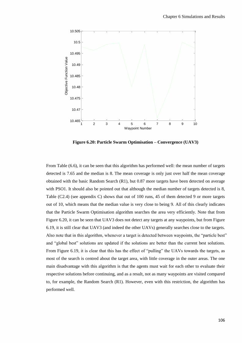
Chapter 6 Simulations and Results
106
Figure 6.20: Particle Swarm Optimisation – Convergence (UAV3)
From Table (6.6), it can be seen that this algorithm has performed well: the mean number of targets
detected is 7.65 and the median is 8. The mean coverage is only just over half the mean coverage
obtained with the basic Random Search (R1), but 0.87 more targets have been detected on average
with PSO1. It should also be pointed out that although the median number of targets detected is 8,
Table (C2.4) (see appendix C) shows that out of 100 runs, 45 of them detected 9 or more targets
out of 10, which means that the median value is very close to being 9. All of this clearly indicates
that the Particle Swarm Optimisation algorithm searches the area very efficiently. Note that from
Figure 6.20, it can be seen that UAV3 does not detect any targets at any waypoints, but from Figure
6.19, it is still clear that UAV3 (and indeed the other UAVs) generally searches close to the targets.
Also note that in this algorithm, whenever a target is detected between waypoints, the “particle best”
and “global best” solutions are updated if the solutions are better than the current best solutions.
From Figure 6.19, it is clear that this has the effect of “pulling” the UAVs towards the targets, as
most of the search is centred about the target area, with little coverage in the outer areas. The one
main disadvantage with this algorithm is that the agents must wait for each other to evaluate their
respective solutions before continuing, and as a result, not as many waypoints are visited compared
to, for example, the Random Search (R1). However, even with this restriction, the algorithm has
performed well.
1 2 3 4 5 6 7 8 9 1010.465
10.47
10.475
10.48
10.485
10.49
10.495
10.5
10.505
Waypoint Number
Obje
ctive F
unction V
alu
e

Chapter 6 Simulations and Results
107
6.4.4 Genetic Algorithm – Elitist
The final nature-inspired heuristic technique to be tested is the Genetic Algorithm. In particular,
this section tests Genetic Algorithms using the Elitist selection method. The Genetic Algorithms
are implemented by letting the vehicles represent the “population”. The UAVs are assigned random
initial positions to initialise the population, and from that point, the Genetic Algorithm takes over.
When the Elitist method is used, it is guaranteed that there is at least one solution in the current
population present in the next generation, so if the population size is equal to the number of
vehicles, then at least one of them does not have to travel at all during the evaluation of the next
generation. Therefore, the population size is taken to be one more than the number of vehicles, and
the one elite individual is carried through to the following generation. Also, target detections
between waypoints are incorporated into the algorithm by using the target location as the
corresponding offspring solution instead of the waypoint (unless there is a target at the waypoint).
In the context of Genetic Algorithms, this can be interpreted as a mutation. In this section, two
variations of Genetic Algorithm (GA) using the Elitist selection method are tested: GA with 5%
mutation rate (GA1_E_5), and GA with 20% mutation rate (GA1_E_20). The results for these two
variations are summarised in Table (6.7).
Table 6.7: Genetic Algorithm – Elitist – Results
Algorithm Targets Detected % Coverage Detection Time (s)
Mean Median St. Dev. Mean Median St. Dev. Mean Median St. Dev.
GA1_E_5 6.46 7 2.68 25.22 24.90 4.38 122.19 69.58 130.19
GA1_E_20 6.72 7 2.20 31.50 31.57 3.83 107.35 69.58 94.15
A typical run of the Elitist Genetic Algorithm with a 5% mutation rate (GA1_E_5) is shown in
Figure 6.21. The maximum value of the objective function at each generation is shown in Figure
6.22. Note that this excludes the “elite” individual to give an indication of the other solutions
generated.

Chapter 6 Simulations and Results
108
Figure 6.21: Genetic Algorithm – Elitist – 5% Mutation
Figure 6.22: Genetic Algorithm – Elitist – 5% Mutation – Convergence
In this case, the mean number of targets detected is 6.46 and the mean coverage is 25.22%, which
appears reasonable at first glance. However, it should be pointed out that several simulations
-250 -200 -150 -100 -50 0 50 100 150 200 250-250
-200
-150
-100
-50
0
50
100
150
200
250
East Position [m]
Nort
h P
ositio
n [
m]
UAV1 UAV2 UAV3 UAV4 Targets Boundary Waypoints
1 2 3 4 5 6 7 8 910
15
20
25
30
35
40
Generation
Maxim
um
Fitness

Chapter 6 Simulations and Results
109
resulted in a low number of targets being detected: 8 of them detected no more than 1 target, which
indicates that there is not enough diversity in this particular algorithm. From the waypoints
generated in Figure 6.21, many of them are close together and a number of them are close to targets,
but there are also numerous waypoints that have been generated away from the targets, and there is
no obvious convergence pattern. From Figure 6.22, even when there are target locations in one
generation, this does not guarantee good solutions in the next generation, as there are instances of
the best solution in one generation being at a target, with no such solutions in the next generation. It
appears that the small population (in this case, 5) prevents this algorithm from showing the typical
characteristics of Genetic Algorithms, like convergence of the population to good solutions.
The mutation rate is now increased to 20%, and a typical run of this Elitist Genetic Algorithm with
a 20% mutation rate (GA1_E_20) is shown in Figure 6.23. The maximum value of the objective
function at each generation is shown in Figure 6.24. Again, this excludes the “elite” individual.
Figure 6.23: Genetic Algorithm – Elitist – 20% Mutation
-250 -200 -150 -100 -50 0 50 100 150 200 250-250
-200
-150
-100
-50
0
50
100
150
200
250
East Position [m]
Nort
h P
ositio
n [
m]
UAV1 UAV2 UAV3 UAV4 Targets Boundary Waypoints

Chapter 6 Simulations and Results
110
Figure 6.24: Genetic Algorithm – Elitist – 20% Mutation – Convergence
With a higher mutation rate, the mean coverage has increased (compared to GA1_E_5) from
25.22% to 31.50%, and only 4 (as opposed to 8 with GA1_E_5) simulations have resulted in no
more than 1 target being detected. This is exactly what would be expected, as a higher mutation
rate corresponds to more diversity in the solutions. Indeed, from Figure 6.23, the range of
waypoints is more diverse than for GA1_E_5 (Figure 6.21). The mean number of targets detected
has increased slightly (6.46 to 6.72) but not significantly. From Figure 6.23, a handful of waypoints
are close to the targets but again, many of them are far away from the targets. This indicates that
there is the potential for the crossover operation to reproduce good solutions but there is also the
potential for many good solutions to be destroyed. This observation can also be made from Figure
6.24: some good solutions have been produced in consecutive generations, but there is still no
guarantee of the good solutions remaining in the population. This is partly due to the objective
function being virtually constant across most of the search space (except at the targets), since a
point just along from a target may have the same objective function value as a point that is very far
away from any targets. The loss of good solutions can also be explained by mutation and the small
population.
1 2 3 4 5 6 7 810
15
20
25
30
35
40
Generation
Maxim
um
Fitness

Chapter 6 Simulations and Results
111
6.4.5 Genetic Algorithm – Roulette Wheel
This section investigates the impact of Genetic Algorithms using the Roulette Wheel selection
method. With the Roulette Wheel method, the population size is simply taken to be the number of
vehicles. The implementation of the Roulette Wheel is straightforward, with each solution taking
up the appropriate space in the “Roulette Wheel”, and the parents selected accordingly (with
probability directly proportional to fitness). Also, like the Elitist method, target detections between
waypoints are incorporated into the algorithm by using the target location as the corresponding
offspring solution instead of the waypoint (unless there is a target at the waypoint). In this section,
two variations of Genetic Algorithm (GA) using the Roulette Wheel selection method are tested:
GA with 5% mutation rate (GA1_RW_5), and GA with 20% mutation rate (GA1_RW_20). The
results for these two variations are summarised in Table (6.8).
Table 6.8: Genetic Algorithm – Roulette Wheel – Results
Algorithm Targets Detected % Coverage Detection Time (s)
Mean Median St. Dev. Mean Median St. Dev. Mean Median St. Dev.
GA1_RW_5 6.64 8 3.07 25.86 26.01 4.83 137.94 69.58 145.29
GA1_RW_20 6.48 7 2.45 31.87 31.94 3.71 115.34 69.58 112.53
A typical run of the Roulette Wheel Genetic Algorithm with a 5% mutation rate (GA1_RW_5) is
shown in Figure 6.25. The maximum value of the objective function at each generation is shown in
Figure 6.26.
Figure 6.25: Genetic Algorithm – Roulette Wheel – 5% Mutation
-250 -200 -150 -100 -50 0 50 100 150 200 250-250
-200
-150
-100
-50
0
50
100
150
200
250
East Position [m]
Nort
h P
ositio
n [
m]
UAV1 UAV2 UAV3 UAV4 Targets Boundary Waypoints

Chapter 6 Simulations and Results
112
Figure 6.26: Genetic Algorithm – Roulette Wheel – 5% Mutation – Convergence
This algorithm has performed very similarly to the Elitist method (GA1_E_5) in terms of target
detection, with only marginal increases in target detection and coverage. Like the Elitist method,
Figure 6.25 shows a handful of waypoints being generated close to the targets, but several
waypoints have still been generated far away from the targets. Figure 6.26 does indicate that good
solutions can reproduce other good solutions using this method, but again, because the population
is so low and the temperature distribution is mostly very flat, there is still the potential for good
solutions to be destroyed between generations. It is also evident that because the mutation rate is
low, the algorithm is somewhat unreliable, since 12 simulations out of 100 have resulted in no
more than 1 target being detected.
The mutation rate is now increased to 20%, and a typical run of this Roulette Wheel Genetic
Algorithm with a 20% mutation rate (GA1_RW_20) is shown in Figure 6.27. The maximum value
of the objective function at each generation is shown in Figure 6.28.
1 2 3 4 5 6 7 8 9 1010
15
20
25
30
35
40
Generation
Maxim
um
Fitness

Chapter 6 Simulations and Results
113
Figure 6.27: Genetic Algorithm – Roulette Wheel – 20% Mutation
Figure 6.28: Genetic Algorithm – Roulette Wheel – 20% Mutation – Convergence
As expected, the higher mutation rate has increased the coverage compared to GA1_RW_5: the
mean has increased from 25.86% to 31.87%. Indeed, comparing Figures 6.25 and 6.27, there is a
-250 -200 -150 -100 -50 0 50 100 150 200 250-250
-200
-150
-100
-50
0
50
100
150
200
250
East Position [m]
Nort
h P
ositio
n [
m]
UAV1 UAV2 UAV3 UAV4 Targets Boundary Waypoints
1 2 3 4 5 6 7 8 910
15
20
25
30
35
40
Generation
Maxim
um
Fitness

Chapter 6 Simulations and Results
114
larger distribution of waypoints in Figure 6.27 because of the higher mutation rate. The mean
number of targets detected has actually decreased slightly from 6.64 to 6.48, but the standard
deviation has decreased from 3.07 to 2.45, indicating that there are fewer very poor simulations
with the higher mutation rate. Indeed, only 4 simulations have resulted in no more than 1 target
being detected, as opposed to 12 with GA1_RW_5. The standard deviation has also decreased in
the coverage and detection time, indicating that the higher mutation rate makes the algorithm
slightly more reliable. Again, there is some evidence of waypoints forming around the targets, but
there are also several waypoints that are far away from the targets. From Figure 6.28, there is still
no guarantee of good solutions remaining in the population from generation to generation, again
because of the small population, the flat temperature distribution, and the scarcity of good solutions.
6.4.6 Genetic Algorithm – Tournament Selection
This section investigates Genetic Algorithms with the third and final selection method: Tournament
Selection. With this method, the population size is simply the number of vehicles. This selection
method has been implemented by holding tournaments consisting of 2 competitors. Any higher
than this would mean that there is more than a 50% chance of the same parent being chosen twice
for a given crossover procedure when only four UAVs are involved in the search. In this section,
two variations of Genetic Algorithm (GA) using the Tournament Selection method are tested: GA
with 5% mutation rate (GA1_TS_5), and GA with 20% mutation rate (GA1_TS_20). The results
for these two variations are summarised in Table (6.9).
Table 6.9: Genetic Algorithm – Tournament Selection – Results
Algorithm Targets Detected % Coverage Detection Time (s)
Mean Median St. Dev. Mean Median St. Dev. Mean Median St. Dev.
GA1_TS_5 6.67 8 2.91 25.84 25.58 5.26 127.41 69.58 134.75
GA1_TS_20 6.20 7 2.53 32.47 32.83 3.60 114.48 69.60 103.17
A typical run of the Tournament Selection Genetic Algorithm with a 5% mutation rate
(GA1_TS_5) is shown in Figure 6.29. The maximum value of the objective function at each
generation is shown in Figure 6.30.

Chapter 6 Simulations and Results
115
Figure 6.29: Genetic Algorithm – Tournament Selection – 5% Mutation
Figure 6.30: Genetic Algorithm – Tournament Selection – 5% Mutation – Convergence
From these results, the Tournament Selection method has performed similarly to the corresponding
algorithms for the Elitist and Roulette Wheel selection methods (GA1_E_5 and GA1_RW_5
-250 -200 -150 -100 -50 0 50 100 150 200 250-250
-200
-150
-100
-50
0
50
100
150
200
250
East Position [m]
Nort
h P
ositio
n [
m]
UAV1 UAV2 UAV3 UAV4 Targets Boundary Waypoints
1 2 3 4 5 6 7 8 910
15
20
25
30
35
40
Generation
Maxim
um
Fitness

Chapter 6 Simulations and Results
116
respectively), with target detection, coverage, and time of first detection staying virtually the same.
Again though, the low mutation rate results in several poor simulations, with 10 in this case
detecting no more than 1 target. On a more positive note, from Figure 6.29, there is more evidence
(in this particular case) of the waypoints clustering around the targets compared to the other
selection methods. This is because with Tournament Selection, the winners of each tournament are
always chosen for crossover, whereas with the Elitist method, there is no guarantee of the best
solution(s) being chosen for crossover. Also, with the Roulette Wheel method, the selection process
is more random and again, there is no guarantee of good solutions being chosen for crossover.
However, the overall conclusion is that the mutation rate is too low for this algorithm to be reliable.
The mutation rate is now increased to 20%, and a typical run of this Tournament Selection Genetic
Algorithm with a 20% mutation rate (GA1_TS_20) is shown in Figure 6.31. The maximum value
of the objective function at each generation is shown in Figure 6.32.
Figure 6.31: Genetic Algorithm – Tournament Selection – 20% Mutation
-250 -200 -150 -100 -50 0 50 100 150 200 250-250
-200
-150
-100
-50
0
50
100
150
200
250
East Position [m]
Nort
h P
ositio
n [
m]
UAV1 UAV2 UAV3 UAV4 Targets Boundary Waypoints

Chapter 6 Simulations and Results
117
Figure 6.32: Genetic Algorithm – Tournament Selection – 20% Mutation – Convergence
With the higher mutation rate, more ground has been covered compared to GA1_TS_5: the mean
coverage has increased to 32.47%. Comparing Figure 6.31 to Figure 6.29 it can be seen that there is
a lot more diversity in this case compared to the 5% mutation rate, hence the higher coverage. This
is also confirmed in Figure 6.32, where it can be seen that good solutions have been destroyed on a
couple of occasions. Although the high mutation rate is likely to be a factor in this, it should be
emphasised once again that the objective function is relatively flat, except for a few peaks at the
target locations. Therefore, a point that is only a few metres away from a target is not considered a
“good” solution in this context, even though realistically it should be considered a good solution.
This, as well as the low population, also has an effect on the convergence. In terms of target
detection, the mean has decreased slightly but the standard deviation has also decreased, indicating
that there are fewer poor runs with the higher mutation rate. This is indeed the case, with 6
simulations resulting in no more than 1 target detection, as opposed to GA1_TS_5, where there
were 10 such simulations. Therefore, the higher mutation rate makes the algorithm more reliable in
terms of producing fewer poor runs.
1 2 3 4 5 6 7 8 910
15
20
25
30
35
40
Generation
Maxim
um
Fitness

Chapter 6 Simulations and Results
118
6.5 Comparison of Search Algorithms
The performance of the search algorithms is evaluated in terms of number of targets detected,
coverage of search space, and detection time. The values for each of these metrics for all the
algorithms tested in this chapter are given in Table (6.10).
Table 6.10: Comparison of Search Algorithms
Algorithm Targets Detected % Coverage Detection Time (s)
Mean Median St. Dev. Mean Median St. Dev. Mean Median St. Dev.
PS 5.58 6 1.79 46.48 46.45 0.13 86.51 61.10 58.64
SS 5.27 5 1.74 43.32 43.32 0.06 82.88 60.90 71.60
ES 5.58 6 1.75 47.43 47.44 0.14 112.86 64.72 97.19
R1 6.78 7 1.99 46.46 46.60 1.93 83.86 65.68 59.46
DR_R1 5.02 5 2.26 41.38 41.67 1.79 112.02 62.56 113.78
ACO1 4.89 5 3.21 25.86 25.92 2.47 166.58 69.62 173.77
PSO1 7.65 8 2.48 26.30 26.32 3.45 109.31 69.58 113.44
GA1_E_5 6.46 7 2.68 25.22 24.90 4.38 122.19 69.58 130.19
GA1_E_20 6.72 7 2.20 31.50 31.57 3.83 107.35 69.58 94.15
GA1_RW_5 6.64 8 3.07 25.86 26.01 4.83 137.94 69.58 145.29
GA1_RW_20 6.48 7 2.45 31.87 31.94 3.71 115.34 69.58 112.53
GA1_TS_5 6.67 8 2.91 25.84 25.58 5.26 127.41 69.58 134.75
GA1_TS_20 6.20 7 2.53 32.47 32.83 3.60 114.48 69.60 103.17
Out of the three standard search patterns (PS, SS, and ES), the Expanding Square method has the
highest coverage, although it also takes longest on average to detect the first target. As explained,
this is because the UAVs start at a slow speed to enable them to trace the path of such a small
square and as a result, this method takes longer to get started. Nevertheless, over the full simulation
time, the mean number of targets detected is higher than Sector Search and exactly the same as
Parallel Sweep. The Sector Search method gives the lowest coverage out of the three and
consequently, detects the fewest targets on average. The reason for the lower coverage is that this
particular search visits points that have already been searched (around the centre point for each
individual vehicle) whereas the other methods are less prone to visiting the same point more than
once until later on in the search. Out of the three methods, the Sector Search method is the quickest
in terms of detecting the first target, although Parallel Sweep is very similar in this respect. This is
because these methods start quickly and cover a wide range of points at the start of the search. It
should also be pointed out that the results for the Parallel Sweep and Expanding Square are very
similar when it comes to coverage and target detection, although Parallel Sweep is generally a lot
quicker at detecting the first target.
Most of the other algorithms have given reasonable performances, with the exceptions being the
Random Search in Distinct Regions, and Ant Colony Optimisation. It has been found that the
distinct regions restrict the agents and therefore, fewer targets are detected (than the Random

Chapter 6 Simulations and Results
119
Search R1), and with Ant Colony Optimisation, the “pheromones” do not draw the agents towards
the targets enough, and it has generally been found to be unreliable. In terms of target detection, the
Random Search and all of the Genetic Algorithms have given very similar average results, but with
none of them really standing out. When observing the standard deviation of the number of targets
detected and also the coverage and detection time, it has been found however that the Random
Search is a lot more reliable than the Genetic Algorithms, in the sense that there is less chance of
the Random Search producing a very poor run. It could also be inferred that the Genetic
Algorithms are much more reliable with the 20% mutation rate than with the 5% mutation rate.
This is reinforced by the greater coverage for all of the Genetic Algorithms when the 20% mutation
rate is used. Based on these observations, it has been decided not to test the 5% mutation rates in
future simulations in this thesis.
Although the Random Search is more reliable than Genetic Algorithms in the sense that it produces
fewer poor runs, it has the disadvantage that it has no memory and doesn’t use information gained
throughout the search to find other targets. This can be observed when examining the number of
targets detected compared to the coverage: with the Random Search, a mean of 6.78 targets are
detected with a mean coverage of 46.46%, while, for example, the Genetic Algorithm using the
Elitist selection method with a 20% mutation rate detects a mean of 6.72 targets with a mean
coverage of only 31.50%. However, the Random Search has the advantage that it generally detects
targets more quickly than most other algorithms due to its diversity: the mean detection time is the
second lowest out of all these algorithms (it is just under a second more than Sector Search), and
the standard deviation is also the second lowest (it is just under a second more than Parallel Sweep),
indicating that it is very reliable at finding targets quickly.
Based on the number of targets detected, the heuristics do generally appear to have an advantage
over the standard search patterns, but the only algorithm that really stands out in this sense is
Particle Swarm Optimisation: the mean number of targets detected is 7.65, which is greater than
that of all the other algorithms by a considerable margin. The structure of this algorithm appears to
be beneficial to this type of problem, with the agents typically being drawn towards the target areas,
with enough diversity to prevent the algorithm getting stuck.
6.6 Summary
This chapter presented the setup of the simulations of an air-sea search mission involving four
UAVs, and how the various search techniques were implemented. The results of these techniques
were also given, and these results were analysed.

Chapter 6 Simulations and Results
120
First of all, three standard search techniques were tested: Parallel Sweep, Sector Search, and
Expanding Square. It was found that the Parallel Sweep method usually made the first detection in
the fastest time, although the Expanding Square method covered slightly more ground. The Sector
Search covered the least ground and detected the fewest targets, since parts of the search space
were covered more than once with this method. However, it was the Expanding Square method
that took the longest time to detect the first target due to its slow start. The Parallel Sweep and
Expanding Square methods detected the equal highest number of targets on average (out of the
three standard search methods), which reflects the similar coverage obtained from each of these
methods.
After testing the common search patterns, several optimisation techniques were tested. The only
algorithm that covered a similar portion of the search space to the standard methods was the
Random Search (the basic form (R1) and also when assigning the four UAVs to distinct regions
(DR_R1)). However, many of the optimisation techniques did perform better than the standard
search methods in terms of target detection, including Particle Swarm Optimisation and some of
the Genetic Algorithms. The best algorithm in terms of target detection was Particle Swarm
Optimisation (PSO1), which detected an average of 7.65 targets on every run.
The basic Random Search (R1) performed reasonably well, covering a similar amount of ground as
the standard search methods, but detecting more targets. As explained, this is due to the higher
likelihood of the Random Search covering more of the central region, where the targets happen to
be located in the simulations. It was found that the distinct regions restricted the agents, and this
variation of the Random Search did not cover quite as much ground and did not detect as many
targets.
Ant Colony Optimisation did not perform particularly well, with the pheromones not having the
intended effect of pulling the agents towards them. This was partly due to the time constraints
imposed by fuel consumption, but also because of the low number of agents. Since time is possibly
a factor, Appendix D1 shows some results for this algorithm with the simulation time extended to
15 minutes. Overall though, in this section, this particular method appears to be unreliable.
The Genetic Algorithms gave reasonable average results, but did not get a chance to develop
properly because of the low population size, time constraints, and the flatness of the objective
function, and therefore it was difficult to fully analyse the convergence patterns. For this reason,
like Ant Colony Optimisation, some results are shown in Appendix D1 with the simulation time
extended to 15 minutes. For all the Genetic Algorithms, it was found that the 5% mutation was too
low, and often resulted in no targets being detected, whereas the 20% mutation rate provided more
randomness and diversity to the search. The high standard deviations with the 5% mutation rates
illustrate the unreliability when this low mutation rate is used.

Chapter 6 Simulations and Results
121
The Particle Swarm Optimisation method (PSO1) detected the most targets on average, and
performed well most of the time, apart from a few poor runs. It was found that updating the
“particle best” and “global best” solutions had the intended effect of drawing the agents towards
the targets.
It should be pointed out that for all of these algorithms, the vast majority of target detections
occurred as the agents were travelling between waypoints, as clearly illustrated by the Objective
Function plots, but these detections were incorporated into the heuristic algorithms to allow them to
search in more promising areas, as opposed to the Random Search, which does not use any of this
information to influence the remainder of the search. The heuristics did often have the intended
effect of allowing the search to take place near the targets. Therefore, even if the waypoints were
not generated at the targets, there was still a good chance of them being detected as they were in the
right area to do so. This was reflected in the results presented, as the objective function at various
waypoints usually only indicated the temperature of the sea, but trajectories often showed the
agents searching close to targets. This observation is a clear justification for keeping the cameras
switched on for the entire search.
Overall, several algorithms surpassed the benchmark set by the standard search patterns in terms of
target detection, although only the Random Searches covered as much ground. The algorithm that
detected the most targets on average was Particle Swarm Optimisation.

Chapter 7 Simulations and Results: Guided Search Algorithms
122
Chapter 7
Simulations and Results: Guided Search Algorithms
7.1 Introduction
This chapter shows the results of the optimisation techniques when they are guided by means of a
probability distribution. In Chapter 6, the search methods were tested using temperature as the
objective function. However, for several algorithms, using temperature on its own as an objective
function is not an effective method of detecting survivors. This is because the temperature
distribution across the search space is mostly flat, as the targets are very small in comparison to the
search area. This is illustrated in Figure 7.1, where 10 targets are placed in a 400m by 400m square.
Figure 7.1: Search Space Temperature Distribution
The scarcity of good solutions was made very clear by the Objective Function plots in Chapter 6.
However, if the location of the accident is known, then the survivors are likely to be located quite
close to this location, as opposed to being scattered randomly throughout the search region.

Chapter 7 Simulations and Results: Guided Search Algorithms
123
Therefore, it would be beneficial to construct a probability map, indicating the likely positions of
the targets, and using this information as part of the objective function to create larger target
footprints. This chapter describes the setup of the probability distribution, how it is applied to the
search algorithms, and the results of these algorithms.
Section 7.2 presents the details of the probability distribution and how it is included in the objective
function. The results and analysis of the guided search algorithms are presented in Section 7.3.
Section 7.4 compares these search algorithms, and finally, Section 7.5 summarises the chapter.
7.2 Probability Distribution
In the simulations, most of the targets are expected to be reasonably close to the accident, with
possibly a few being located a little bit further away. Therefore, if a target is found, it is likely that
there are other targets nearby, so it would be beneficial to update the objective function to reflect
this. Also, at the start of the search, the targets are expected to be closer to the origin than at the
edge of the search area, since the simulations are set up so that the reported ship sinking is around
the origin. Therefore, a probability element of the following form can be included in the objective
function at the start of the simulations:
222 2σyxCeyx,P (7.1)
Here, C is a constant, which reflects the relative weight between the probability function and the
temperature reading, and σ is the standard deviation of the distribution, which reflects the estimated
distribution of the targets, and the uncertainty in the position of the accident. For the simulations
run here, the constant C is taken to be 10, so that the probability map plays a significant role, but
does not overpower high temperature readings, and the standard deviation σ is taken to be 100m, so
that the probability distribution extends far enough to cover the entire search space, and doesn’t
ignore points that are further out. A Gaussian distribution of the form given in Equation (7.2) is
then added to the objective function if a target is found at (x0, y0):
220
20 2σy-yx-x
Ceyx,P
(7.2)
In this case, C is taken to be 20 and σ is taken to be 40m. This specific value of C is chosen so that
it is greater than the value from Equation (7.1), and hence favours the actual locations of targets
rather than an initial guess. The value of σ is chosen as 40m so that the target footprints are much
larger than those formed by the temperature distribution, but small enough that it encourages a
more localised search than would be generated by a large value of σ. It was therefore decided that σ
should be chosen to be 10% of the dimensions of the search space. Even though the target spread is
not known a priori, the general shape of the probability distribution remains the same, which is the

Chapter 7 Simulations and Results: Guided Search Algorithms
124
most important aspect here. The overall objective function is the sum of the temperature and the
probability distribution. Initially, the probability distribution is given by Equation (7.1), and is
updated by adding Equation (7.2) onto it whenever a target is detected (for the first time) at the
point (x0, y0). As an example, Figure 7.2 shows the probability distribution after a detection at the
point (50,50). This clearly shows the larger target footprint created by the probability distribution.
Figure 7.2: Probability Distribution
7.3 Optimisation Techniques and Results
This section shows the results of the optimisation techniques when guided using the probability
distribution as described in Section 7.2. The three standard search patterns (Parallel Sweep, Sector
Search, and Expanding Square) are not tested in this chapter since their paths are predetermined
and are not influenced by any new information gained during the search. Therefore, the probability
distribution makes no difference at all to these algorithms, and therefore, testing them in this
chapter is unnecessary. The individual results for the techniques used in this section are given in
Appendix C3.

Chapter 7 Simulations and Results: Guided Search Algorithms
125
7.3.1 Guided Random Search
The basic Random Search (R1) does not depend on the objective function, since the algorithm does
not use any information gained throughout the search to influence the remainder of the search. The
way in which the probability distribution (as discussed in Section 7.2) is used here is to select the
random points with a probability that reflects this distribution; if a target is found in a certain
position, then the probability around this point is increased (according to Equation (7.2), with a
normalised probability calculated afterwards), which makes the selection of a nearby point more
likely. This probability distribution allows a more guided search to take place. In this section, two
variations of the Guided Random Search are tested: the Guided Random Search (R2), and the
Guided Random Search in Distinct Regions (DR_R2). The results for these two variations are
summarised in Table (7.1).
Table 7.1: Guided Random Search – Results
Algorithm Targets Detected % Coverage Detection Time (s)
Mean Median St. Dev. Mean Median St. Dev. Mean Median St. Dev.
R2 8.74 9 1.82 30.96 30.69 3.68 90.39 61.80 87.96
DR_R2 7.25 8 1.70 32.64 33.12 3.13 90.01 65.70 68.98
A typical run of the Guided Random Search (R2) is shown in Figure 7.3. The value of the objective
function at each waypoint for UAV3 is shown in Figure 7.4.
Figure 7.3: Guided Random Search
-250 -200 -150 -100 -50 0 50 100 150 200 250-250
-200
-150
-100
-50
0
50
100
150
200
250
East Position [m]
Nort
h P
ositio
n [
m]
UAV1 UAV2 UAV3 UAV4 Targets Boundary Waypoints

Chapter 7 Simulations and Results: Guided Search Algorithms
126
Figure 7.4: Guided Random Search – Convergence (UAV3)
Figure 7.3 shows that this algorithm performs very well, with many of the selected waypoints
clustering around the detected targets. This can be backed up by the results in Table (7.1): the mean
number of targets detected is 8.74 and the median is 9, indicating that 9 or more targets have been
detected in at least 50% of the runs. This is a clear improvement on the basic Random Search (R1),
which detected 6.78 targets on average. The coverage in this case is significantly lower than R1.
However, the coverage is lower for a very good reason: this algorithm is trying to search around the
targets that have already been detected instead of carrying out a search with no memory. This
algorithm clearly favours an intense search in promising areas over a diverse search over the entire
area. Indeed, Figure 7.4 indicates that UAV3 hones in on targets as the search goes on, as the
objective function value generally increases over successive waypoints, which would only be the
case if the search is being carried out around the targets.
The Guided Random Search is now tested in Distinct Regions: a typical run of this algorithm
(DR_R2) is shown in Figure 7.5. The value of the objective function at each waypoint for UAV3 is
shown in Figure 7.6.
1 2 3 4 5 6 7 8 9 10 11 12 13 14 150
20
40
60
80
100
120
140
160
180
Waypoint Number
Obje
ctive F
unction V
alu
e

Chapter 7 Simulations and Results: Guided Search Algorithms
127
Figure 7.5: Guided Distinct Regions Random Search
Figure 7.6: Guided Distinct Regions Random Search – Convergence (UAV3)
In terms of target detection, this method has performed significantly better than DR_R1 (the non-
Guided Random Search in Distinct Regions), detecting an extra 2.23 targets per run on average.
-250 -200 -150 -100 -50 0 50 100 150 200 250-250
-200
-150
-100
-50
0
50
100
150
200
250
East Position [m]
Nort
h P
ositio
n [
m]
UAV1 UAV2 UAV3 UAV4 Targets Boundary Waypoints
1 2 3 4 5 6 7 8 9 10 11 12 13 14 15 16 170
20
40
60
80
100
120
140
Waypoint Number
Obje
ctive F
unction V
alu
e

Chapter 7 Simulations and Results: Guided Search Algorithms
128
This has also been achieved with a lower coverage, for the same reason that R2 covers less ground
than R1: this algorithm causes agents to hone in on promising areas, as opposed to DR_R1, which
merely provides a random, distributed search. However, compared to R2, using distinct regions has
not proved to be beneficial, since the mean and median number of targets detected are both lower
for DR_R2, despite the coverage being slightly higher. When a target is detected, the probability
distribution is increased, but when the UAVs are constrained to particular regions, only the UAV
searching that region is likely to be drawn towards that area, whereas in R2, all the UAVs are likely
to be drawn towards the target. As a result, R2 carries out a more intense search of the target area
than DR_R2. This explains why for DR_R2, fewer targets have been detected despite more ground
being covered. Figure 7.6 does indicate a “honing in” effect with the increasing objective function,
but this only applies to UAV3 in this case (see Figure 7.5), as the other three UAVs do not detect
any targets.
7.3.2 Guided Hill Climbing
The Hill Climbing algorithm is implemented by generating random starting points, and then
performing the local searches around those points. The local search is carried out by selecting a
random point within 100 metres (but no less than 10 metres, due to the detection diameter of the
camera) of the current point, and evaluating the solution. The algorithm has also been tested with
the local search being carried out within 20 metres of the current point, but it has been found that
this does not allow much of a search to take place, as illustrated in Appendix D2. Therefore, it has
been decided to carry out the local search within 100 metres of the current point. Note that targets
detected between waypoints are incorporated into the algorithm as described in Section 6.2.2, with
the “current solution” being updated to the target location to allow the next part of search to take
place in that area. The Random Restart Hill Climbing algorithm is also implemented in exactly the
same way as Hill Climbing, except for the Random Restart condition. The Random Restart is
triggered if more than 5 consecutive solutions are evaluated without improvement. This is done to
prevent the algorithm getting stuck at local maxima.
Two variations of the Guided Hill Climbing algorithm are tested in this section: the Guided Hill
Climbing algorithm (HC2), and the Guided Random Restart Hill Climbing algorithm (RR_HC2).
Note that like the Random Search, Hill Climbing could also be tested using distinct regions, but
since this did not have any positive impact on the results of the Random Search, it was decided that
this should be omitted. The results for these two variations are summarised in Table (7.2). A typical
run of the Guided Hill Climbing algorithm (HC2) is shown in Figure 7.7. The value of the
objective function at each waypoint for UAV3 is shown in Figure 7.8.
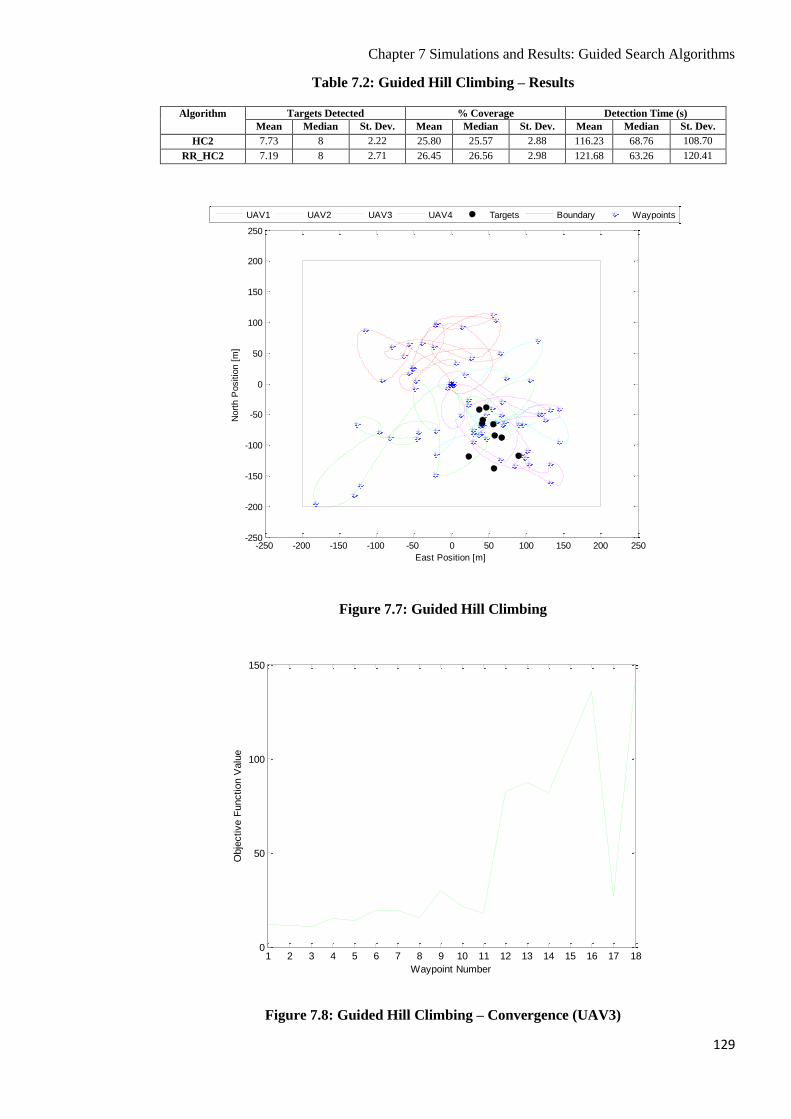
Chapter 7 Simulations and Results: Guided Search Algorithms
129
Table 7.2: Guided Hill Climbing – Results
Algorithm Targets Detected % Coverage Detection Time (s)
Mean Median St. Dev. Mean Median St. Dev. Mean Median St. Dev.
HC2 7.73 8 2.22 25.80 25.57 2.88 116.23 68.76 108.70
RR_HC2 7.19 8 2.71 26.45 26.56 2.98 121.68 63.26 120.41
Figure 7.7: Guided Hill Climbing
Figure 7.8: Guided Hill Climbing – Convergence (UAV3)
-250 -200 -150 -100 -50 0 50 100 150 200 250-250
-200
-150
-100
-50
0
50
100
150
200
250
East Position [m]
Nort
h P
ositio
n [
m]
UAV1 UAV2 UAV3 UAV4 Targets Boundary Waypoints
1 2 3 4 5 6 7 8 9 10 11 12 13 14 15 16 17 180
50
100
150
Waypoint Number
Obje
ctive F
unction V
alu
e

Chapter 7 Simulations and Results: Guided Search Algorithms
130
From these results, the Guided Hill Climbing algorithm has performed well, with a mean of 7.73
targets detected on every run. The coverage is relatively low because it is a local search and also,
the agents are “pulled” in particular directions due to the probability distribution, thus reducing the
random factor. This gives a clear indication that guiding the search using the probability
distribution is beneficial in this case, as this algorithm encourages an intense search in promising
areas. From Figure 7.7, and also from Figure 7.8, it can be seen that UAV3 starts away from the
targets, and is drawn more towards the target areas as they are detected. In fact, from Figure 7.7,
there is evidence of several agents (all but UAV1) being drawn towards the target locations. Even
though Hill Climbing is a local search algorithm, using the probability distribution ensures that
when one agent detects a target, many of the other agents are drawn towards that area, whereas
without the probability distribution, this would not be the case as the target footprint would be too
small.
A typical run of the Guided Random Restart Hill Climbing algorithm (RR_HC2) is shown in
Figure 7.9. The value of the objective function at each waypoint for UAV4 is shown in Figure 7.10.
Figure 7.9: Guided Random Restart Hill Climbing
-250 -200 -150 -100 -50 0 50 100 150 200 250-250
-200
-150
-100
-50
0
50
100
150
200
250
East Position [m]
Nort
h P
ositio
n [
m]
UAV1 UAV2 UAV3 UAV4 Targets Boundary Waypoints

Chapter 7 Simulations and Results: Guided Search Algorithms
131
Figure 7.10: Guided Random Restart Hill Climbing – Convergence (UAV4)
Compared to HC2, the coverage is only slightly higher as it appears that the Random Restart has
not been triggered very often. This is due to the lack of local maxima away from the targets, and
because the local search is large enough to detect other targets even when the agent is close to a
local maximum. The mean number of targets detected by this algorithm is actually lower than HC2,
although this difference is very small. Nevertheless, the results do suggest that the Random Restart
makes little difference to the algorithm. In the simulation shown in Figure 7.9, there is evidence of
clustering around the targets as there is with HC2, and from Figure 7.10, UAV4 does gradually
move towards the target locations, as the objective function value generally increases throughout
the simulation.
7.3.3 Guided Simulated Annealing
This section now investigates Simulated Annealing, which is implemented in a very similar way to
Hill Climbing i.e. the initial points are generated in the same way, target detections between
waypoints are incorporated into the algorithm in the same way, and the local solutions are
generated in a similar fashion. The only difference in the local solutions is that the size of the
perturbations decreases with temperature. The Metropolis Procedure is implemented using the
criteria that if the current effective temperature is T and the negative change in the objective
function is ΔF, then the new solution is accepted with probability given by
1 2 3 4 5 6 7 8 9 10 11 12 13 14 150
50
100
150
Waypoint Number
Obje
ctive F
unction V
alu
e

Chapter 7 Simulations and Results: Guided Search Algorithms
132
P = exp(30ΔF/T) (7.3)
Note that there is no negative sign inside the exponential because the objective function here must
be maximised, as opposed to the energy state in annealing, which must be minimised. The 30 is
simply a scaling factor based on the values used for the objective function and the effective
temperature. With this scaling factor in place, there is a 74% chance that a solution that is poorer by
1 (in terms of the value of the objective function) is accepted at the start, where the effective
temperature is taken to be 100, which is a reasonable condition. This effective temperature is
decreased at each iteration by changing T to αT, where α = 0.9. The size of the perturbations at
temperature T is given by
10rand1.9TPert (7.4)
Thus, the initial perturbations can be anything from 10m to 200m (N.B. a minimum of 10m is used
because this is the detection diameter of the camera). After, for example, 25 waypoints, the
perturbation can be anything from 10m to 23.6m, where the fine-tuning takes place.
The Random Restart Simulated Annealing algorithm is also implemented in exactly the same way
as Simulated Annealing, except for the Random Restart condition. Like Hill Climbing, the Random
Restart is triggered if more than 5 consecutive solutions are evaluated without a change in the
“current solution”.
In this section, two variations of the Guided Simulated Annealing algorithm are tested: the Guided
Simulated Annealing algorithm (SA2), and the Guided Random Restart Simulated Annealing
algorithm (RR_SA2). The results for these two variations are summarised in Table (7.3).
Table 7.3: Guided Simulated Annealing – Results
Algorithm Targets Detected % Coverage Detection Time (s)
Mean Median St. Dev. Mean Median St. Dev. Mean Median St. Dev.
SA2 7.36 8 2.82 26.88 26.89 2.58 123.08 67.70 139.32
RR_SA2 7.76 8 2.52 27.99 28.02 2.62 113.52 62.30 122.43
A typical run of the Guided Simulated Annealing algorithm (SA2) is shown in Figure 7.11. The
value of the objective function at each waypoint for UAV4 is shown in Figure 7.12.

Chapter 7 Simulations and Results: Guided Search Algorithms
133
Figure 7.11: Guided Simulated Annealing
Figure 7.12: Guided Simulated Annealing – Convergence (UAV4)
This algorithm has performed very similarly to Hill Climbing, with very similar results for the
number of targets detected, coverage, and time of first detection. The coverage has increased
-250 -200 -150 -100 -50 0 50 100 150 200 250-250
-200
-150
-100
-50
0
50
100
150
200
250
East Position [m]
Nort
h P
ositio
n [
m]
UAV1 UAV2 UAV3 UAV4 Targets Boundary Waypoints
1 2 3 4 5 6 7 8 9 10 11 12 13 14 15 16 1710
20
30
40
50
60
70
80
90
100
110
Waypoint Number
Obje
ctive F
unction V
alu
e

Chapter 7 Simulations and Results: Guided Search Algorithms
134
slightly as expected but by very little, and target detection has barely changed. The algorithm
performs well and like Hill Climbing, it can be seen from Figure 7.11 that several agents are drawn
towards the targets (all but UAV3). This effect is also evident from Figure 7.12, where the
objective function generally increases from waypoint to waypoint, indicating that this particular
UAV is being draw towards the targets. This observation has also been made with Hill Climbing,
and this occurs because when a target is detected, the probability distribution draws other agents
towards that area, whereas without the probability distribution, only the agent that detected the
target would be influenced by the detection due to the small target footprint.
A typical run of the Guided Random Restart Simulated Annealing algorithm (RR_SA2) is shown in
Figure 7.13. The value of the objective function at each waypoint for UAV3 is shown in Figure
7.14.
Figure 7.13: Guided Random Restart Simulated Annealing
-250 -200 -150 -100 -50 0 50 100 150 200 250-250
-200
-150
-100
-50
0
50
100
150
200
250
East Position [m]
Nort
h P
ositio
n [
m]
UAV1 UAV2 UAV3 UAV4 Targets Boundary Waypoints

Chapter 7 Simulations and Results: Guided Search Algorithms
135
Figure 7.14: Guided Random Restart Simulated Annealing – Convergence (UAV3)
Like Hill Climbing, the Random Restart has had little impact on the search: in this case, target
detection and coverage have improved slightly, but these improvements are very insignificant.
Nevertheless, the performance of this algorithm is still reasonably good. Figures 7.13 and 7.14
indicate the “honing in” effect of the probability distribution, with UAV2 and UAV3 clustering
around the targets, and the objective function value generally increasing for UAV3 throughout the
search. Again though, it appears that the Random Restart has not been triggered very often, as there
are very few local maxima except the targets themselves. As a result, target detection and coverage
have not really changed.
7.3.4 Guided Ant Colony Optimisation
The probability distribution is now tested on Ant Colony Optimisation. This algorithm is simply
tested in its basic form with the probability distribution (ACO2). The results for this algorithm are
summarised in Table (7.4). A typical run is shown in Figure 7.15. The value of the objective
function at each waypoint for UAV4 is shown in Figure 7.16.
1 2 3 4 5 6 7 8 9 10 11 12 13 14 150
20
40
60
80
100
120
140
Waypoint Number
Obje
ctive F
unction V
alu
e

Chapter 7 Simulations and Results: Guided Search Algorithms
136
Table 7.4: Guided Ant Colony Optimisation – Results
Algorithm Targets Detected % Coverage Detection Time (s)
Mean Median St. Dev. Mean Median St. Dev. Mean Median St. Dev.
ACO2 6.13 8 3.44 23.80 24.31 2.72 150.18 69.18 159.72
Figure 7.15: Guided Ant Colony Optimisation
Figure 7.16: Guided Ant Colony Optimisation – Convergence (UAV4)
-250 -200 -150 -100 -50 0 50 100 150 200 250-250
-200
-150
-100
-50
0
50
100
150
200
250
East Position [m]
Nort
h P
ositio
n [
m]
UAV1 UAV2 UAV3 UAV4 Targets Boundary Waypoints
1 2 3 4 5 6 7 8 9 10 11 12 13 140
20
40
60
80
100
120
140
Waypoint Number
Obje
ctive F
unction V
alu
e

Chapter 7 Simulations and Results: Guided Search Algorithms
137
The results for this algorithm show a clear improvement compared to ACO1 (without the
probability distribution). The coverage has decreased slightly but target detection has improved
noticeably. The reason for the slight decrease in coverage is that with the probability distribution,
the pheromone count is also likely to indicate how close a point is to a target, whereas without the
probability distribution, the pheromone count only indicates the temperature reading. Therefore, the
pheromone count in ACO1 has a more random nature and hence, more ground is covered with
ACO1. However, the structure of the probability distribution has had a positive effect on target
detection, with the mean increasing from 4.89 to 6.13 and the median increasing from 5 to 8.
However, it should be pointed out that the standard deviation for the number of targets detected is
still high, and again illustrates the unreliability of this method. Indeed, 9 simulations have resulted
in no targets being detected. Like ACO1, the problem is that Ant Colony Optimisation is a local
algorithm, and therefore the agents can only be drawn so far. From Figure 7.15, some of the agents
are drawn towards the targets, but others that are further away only search around their current
locations. The objective function value in Figure 7.16 does indicate that UAV4 is drawn towards
the targets, but not to the same extent as for Guided Hill Climbing and Guided Simulated
Annealing.
7.3.5 Guided Particle Swarm Optimisation
This section investigates whether the probability distribution has an impact on Particle Swarm
Optimisation. This algorithm is simply tested in its basic form with the probability distribution
(PSO2). The results for this algorithm are summarised in Table (7.5).
Table 7.5: Guided Particle Swarm Optimisation – Results
Algorithm Targets Detected % Coverage Detection Time (s)
Mean Median St. Dev. Mean Median St. Dev. Mean Median St. Dev.
PSO2 8.16 8 1.86 26.16 26.15 3.87 96.59 69.60 82.08
A typical run is shown in Figure 7.17. The value of the objective function at each waypoint for
UAV1 is shown in Figure 7.18.

Chapter 7 Simulations and Results: Guided Search Algorithms
138
Figure 7.17: Guided Particle Swarm Optimisation
Figure 7.18: Guided Particle Swarm Optimisation – Convergence (UAV1)
This algorithm has performed well, and has shown improvements in target detection compared to
PSO1. The mean number of targets detected has increased by 0.51, but perhaps more significantly,
-250 -200 -150 -100 -50 0 50 100 150 200 250
-250
-200
-150
-100
-50
0
50
100
150
200
250
East Position [m]
Nort
h P
ositio
n [
m]
UAV1 UAV2 UAV3 UAV4 Targets Boundary Waypoints
1 2 3 4 5 6 7 8 9 10 110
20
40
60
80
100
120
Waypoint Number
Obje
ctive F
unction V
alu
e

Chapter 7 Simulations and Results: Guided Search Algorithms
139
the standard deviation has decreased by 0.62, indicating that the algorithm is much more reliable
with the probability distribution. In fact, with PSO1, there were 15 simulations where no more than
5 targets were detected, but with PSO2, there are only 6 such simulations. The greater reliability of
PSO2 is also reflected in the standard deviation of the detection time. In terms of coverage, there is
not much difference compared to PSO1. In this case, like PSO1, there is evidence of clustering
around the targets despite some of the agents starting far away from them. From Figure 7.18, and
indeed Figure 7.17, UAV1 starts away from the targets and is then drawn towards them. In fact,
this is also the case for some of the other agents. Also notice that some of the waypoints are outside
the search region but as explained, the penalty function ensures that the agents are pulled back into
the search region. Overall, the “good” runs are very similar with or without the probability
distribution, but there are far fewer poor runs with the probability distribution, making PSO2 much
more reliable than PSO1.
7.3.6 Guided Genetic Algorithm – Elitist
The effect of the probability distribution on Genetic Algorithms is now investigated. The first
selection method to be tested is the Elitist selection method. In this section, only one variation of
the Guided Genetic Algorithm (GA) using the Elitist selection method is tested: GA with 20%
mutation rate (GA2_E_20). The 5% mutation rate is not tested because as established in Chapter 6,
it has a habit of getting stuck and not detecting many (if any) targets, and is generally unreliable.
The results for this algorithm are summarised in Table (7.6).
Table 7.6: Guided Genetic Algorithm – Elitist – Results
Algorithm Targets Detected % Coverage Detection Time (s)
Mean Median St. Dev. Mean Median St. Dev. Mean Median St. Dev.
GA2_E_20 6.47 7 2.41 31.43 31.28 3.70 101.17 69.58 87.19
A typical run of this algorithm is shown in Figure 7.19. The maximum value of the objective
function at each generation is shown in Figure 7.20. Again, this excludes the “elite” individual.

Chapter 7 Simulations and Results: Guided Search Algorithms
140
Figure 7.19: Guided Genetic Algorithm – Elitist – 20% Mutation
Figure 7.20: Guided Genetic Algorithm – Elitist – 20% Mutation – Convergence
The results for this algorithm are very similar to GA1_E_20, where the probability distribution was
not used. The results are very similar for every parameter, and suggest that in this case, the
-250 -200 -150 -100 -50 0 50 100 150 200 250-250
-200
-150
-100
-50
0
50
100
150
200
250
East Position [m]
Nort
h P
ositio
n [
m]
UAV1 UAV2 UAV3 UAV4 Targets Boundary Waypoints
1 2 3 4 5 6 7 8 90
20
40
60
80
100
120
140
Generation
Maxim
um
Fitness

Chapter 7 Simulations and Results: Guided Search Algorithms
141
probability distribution has little impact on the search. Fundamentally, once a target has been
detected, there is not much difference between GA1_E_20 and GA2_E_20, as the best solution
from this point is always a target location, and the relative values of the objective function for the
other solutions is irrelevant. From Figure 7.20, it can be seen that the increasing objective function
shows better convergence properties than without the probability distribution, since the probability
distribution gives a better indication of how “good” a solution is, but it should also be pointed out
that Figure 7.19 looks very similar in nature to Figure 6.23, which shows a typical run of
GA1_E_20. Therefore, overall, the probability distribution does not really make any difference to
the search in this case.
7.3.7 Guided Genetic Algorithm – Roulette Wheel
In this section, the Roulette Wheel selection method is tested with the Guided Genetic Algorithms.
Like the Elitist method, the Roulette Wheel method is only tested with a 20% mutation rate
(GA2_RW_20). The results for this algorithm are summarised in Table (7.7).
Table 7.7: Guided Genetic Algorithm – Roulette Wheel – Results
Algorithm Targets Detected % Coverage Detection Time (s)
Mean Median St. Dev. Mean Median St. Dev. Mean Median St. Dev.
GA2_RW_20 7.13 8 2.30 30.25 30.44 3.86 107.11 69.58 92.31
A typical run of this algorithm is shown in Figure 7.21. The maximum value of the objective
function at each generation is shown in Figure 7.22.

Chapter 7 Simulations and Results: Guided Search Algorithms
142
Figure 7.21: Guided Genetic Algorithm – Roulette Wheel – 20% Mutation
Figure 7.22: Guided Genetic Algorithm – Roulette Wheel – 20% Mutation – Convergence
Unlike the Elitist method, these results indicate that the Roulette Wheel selection method has
benefitted from the probability distribution, based on the number of targets detected: the mean has
-250 -200 -150 -100 -50 0 50 100 150 200 250-250
-200
-150
-100
-50
0
50
100
150
200
250
East Position [m]
Nort
h P
ositio
n [
m]
UAV1 UAV2 UAV3 UAV4 Targets Boundary Waypoints
1 2 3 4 5 6 7 8 960
70
80
90
100
110
120
Generation
Maxim
um
Fitness

Chapter 7 Simulations and Results: Guided Search Algorithms
143
increased from 6.48 to 7.13 and the median has increased from 7 to 8. The coverage has decreased
very slightly and this is most likely due to the probability distribution causing the search to become
slightly more concentrated around the targets. Given the nature of the Roulette Wheel method, it
would be expected that the probability distribution should have a positive impact on target
detection, since the Roulette Wheel method selects parents for crossover based on relative fitness
(which becomes more apparent with the probability distribution) unlike the other methods, which
simply rank the solutions. In terms of convergence, like the Elitist method, it can be seen from
Figure 7.22 that with the probability distribution, this Genetic Algorithm shows better convergence
properties, with the maximum fitness at each generation generally increasing throughout the search.
7.3.8 Guided Genetic Algorithm – Tournament Selection
The final selection method to be tested with the Guided Genetic Algorithms is Tournament
Selection. Again, this is only tested with a 20% mutation rate (GA2_TS_20). The results for this
algorithm are summarised in Table (7.8).
Table 7.8: Guided Genetic Algorithm – Tournament Selection – Results
Algorithm Targets Detected % Coverage Detection Time (s)
Mean Median St. Dev. Mean Median St. Dev. Mean Median St. Dev.
GA2_TS_20 6.37 7 2.53 30.30 30.29 3.12 104.81 69.60 101.62
A typical run of this algorithm is shown in Figure 7.23. The maximum value of the objective
function at each generation is shown in Figure 7.24.

Chapter 7 Simulations and Results: Guided Search Algorithms
144
Figure 7.23: Guided Genetic Algorithm – Tournament Selection – 20% Mutation
Figure 7.24: Guided Genetic Algorithm – Tournament Selection – 20% Mutation –
Convergence
-250 -200 -150 -100 -50 0 50 100 150 200 250-250
-200
-150
-100
-50
0
50
100
150
200
250
East Position [m]
Nort
h P
ositio
n [
m]
UAV1 UAV2 UAV3 UAV4 Targets Boundary Waypoints
1 2 3 4 5 6 7 8 910
20
30
40
50
60
70
80
Generation
Maxim
um
Fitness

Chapter 7 Simulations and Results: Guided Search Algorithms
145
Like the Elitist method, these results suggest that Tournament Selection does not really benefit
from the probability distribution, since they are very similar to the results for GA1_TS_20, where
the probability distribution was not used. The results are also very similar to GA2_E_20: the Elitist
selection method where the probability distribution was used. Also, the nature of Figure 7.23 is
very similar to that of Figure 6.31, which shows a typical run of GA1_TS_20. From Figure 7.24,
the maximum fitness shows signs of variation due to the high mutation rate and the low population,
but does show a general increasing trend as the agents hone in on the targets, albeit not particularly
well. Overall, like the Elitist method, there is no significant advantage to using the probability
distribution for Tournament Selection.
7.4 Comparison of Guided Search Algorithms
The performance of the search algorithms is evaluated in terms of number of targets detected,
coverage of search space, and detection time. The values for each of these metrics for all the
algorithms tested in this chapter are given in Table (7.9).
Table 7.9: Comparison of Guided Search Algorithms
Algorithm Targets Detected % Coverage Detection Time (s)
Mean Median St. Dev. Mean Median St. Dev. Mean Median St. Dev.
R2 8.74 9 1.82 30.96 30.69 3.68 90.39 61.80 87.96
DR_R2 7.25 8 1.70 32.64 33.12 3.13 90.01 65.70 68.98
HC2 7.73 8 2.22 25.80 25.57 2.88 116.23 68.76 108.70
RR_HC2 7.19 8 2.71 26.45 26.56 2.98 121.68 63.26 120.41
SA2 7.36 8 2.82 26.88 26.89 2.58 123.08 67.70 139.32
RR_SA2 7.76 8 2.52 27.99 28.02 2.62 113.52 62.30 122.43
ACO2 6.13 8 3.44 23.80 24.31 2.72 150.18 69.18 159.72
PSO2 8.16 8 1.86 26.16 26.15 3.87 96.59 69.60 82.08
GA2_E_20 6.47 7 2.41 31.43 31.28 3.70 101.17 69.58 87.19
GA2_RW_20 7.13 8 2.30 30.25 30.44 3.86 107.11 69.58 92.31
GA2_TS_20 6.37 7 2.53 30.30 30.29 3.12 104.81 69.60 101.62
The real standout from Table (7.9) is the Guided Random Search (R2), which has the highest mean
and median number of targets detected out of all the algorithms tested in this chapter (as well as
Chapter 6). It is also a very reliable method, with a low standard deviation in the number of targets
detected. The standard deviation of the Guided Random Search in Distinct Regions is lower, but so
is the mean number of targets detected, and it has been established that the distinct regions are too
restrictive and do not allow the search to be carried out to its full potential. Another algorithm that
has performed very well is Particle Swarm Optimisation, with the second highest (behind R2) mean
number of targets detected out of the algorithms tested in this chapter (and indeed Chapter 6), and
also a similar level of reliability as R2, based on the standard deviation of the number of targets
detected. The worst algorithm out of those tested in this chapter is Ant Colony Optimisation, with

Chapter 7 Simulations and Results: Guided Search Algorithms
146
the lowest mean number of targets detected and also the highest standard deviation. Although there
has been a noticeable improvement from Chapter 6, this algorithm has proved to be very unreliable
at finding numerous targets consistently. As with Chapter 6, the time constraints are a possible
factor, and some results are shown in Appendix D1 with the simulation time extended to 15
minutes.
The Genetic Algorithms performed reasonably well, but the only selection method that has been
influenced positively by the probability distribution is the Roulette Wheel, having detected the
greatest number of targets out of the three selection methods. It has been found that the Elitist and
Tournament Selection methods are not really influenced by the probability distribution since they
simply rank the solutions in order, but with the Roulette Wheel method, the relative fitness of all
the solutions is more important, and the probability distribution has more of an impact on this.
Again though, as in Chapter 6, the time constraints possibly restrict the development of the Genetic
Algorithms, and some results are shown in Appendix D1 with the simulation time extended to 15
minutes.
It has been found that Hill Climbing and Simulated Annealing perform well with the probability
distribution, and even outperform the more complex Genetic Algorithms in terms of target
detection: the mean number of targets detected is higher for every Hill Climbing and Simulated
Annealing algorithm than that of all the Genetic Algorithms in this chapter (and Chapter 6). This
indicates that it is beneficial to have some sort of “local search”, allowing the agents to hone in on
targets. The Random Restart however, has not made much difference to Hill Climbing and
Simulated Annealing based on the above results. There has not been much change in target
detection (in fact, it has decreased for Hill Climbing) as the Random Restart has not been triggered
very often. Although the coverage has increased slightly in both cases, this is very marginal and
there is no obvious advantage to including the Random Restart in the algorithms.
The most reliable methods (in this chapter) for detecting targets consistently quickly are the two
Random Searches (R2 and DR_R2) and Particle Swarm Optimisation, indicating that in order to
detect the initial target quickly, a high random factor is essential. None of the algorithms really
stand out in terms of coverage, but many of them do have the ability to detect numerous targets.
The best overall performance in this chapter is clearly the Guided Random Search (R2), with its
random nature and the structure of the probability distribution combining to great effect.
7.5 Summary
This chapter presented the concept of a probability distribution, which was used to give an
indication of the likelihood of finding targets in a given area. In Chapter 6, the objective function

Chapter 7 Simulations and Results: Guided Search Algorithms
147
consisted solely of the temperature reading, but because the target footprints were so small, this did
not give much indication of whether or not there may be targets nearby. With the probability
distribution, whenever a target was detected, a probability element was added to the objective
function, and this probability element had a much larger footprint than the target itself. Therefore,
with the probability distribution, there is a clearer indication of the likely locations of targets.
It was found that there was a significant improvement in target detection for the Random Search
compared to that which was tested in Chapter 6. In this algorithm, there was clear evidence that the
probability distribution had the effect of pulling the agents towards the target areas, with many of
the waypoints being generated in promising areas. It was found that due to the probability
distribution, the target areas were searched more intensely instead of the agents performing a
distributed search of the entire area. Therefore, the coverage decreased significantly, but there was
also a major improvement in target detection as a result. It was found once again though that the
Distinct Regions approach did not improve the search as this restricted the possible paths of the
agents. In particular, agents that would otherwise have been drawn towards target areas were forced
to stay in their allotted region, thus preventing them from detecting targets.
With Hill Climbing and Simulated Annealing, it was found that the probability distribution added a
lot of direction to the search, and the agents were therefore directed towards the targets. One
significant effect of the probability distribution was that when a target was detected, many of the
other agents were drawn towards this area as a result, despite all the agents searching independently.
It was observed however that the Random Restart was not triggered very often and hence, this did
not often make a significant difference.
From the results presented in this chapter, the probability distribution also had a positive effect on
Ant Colony Optimisation and Particle Swarm Optimisation. With Ant Colony Optimisation, target
detection improved considerably but it was still found to be very unreliable as there were still a
large number of poor runs. With Particle Swarm Optimisation, target detection improved slightly
but the main impact of the probability distribution was that it improved the reliability of the
algorithm in the sense that there were far fewer poor runs compared to Chapter 6.
With the Genetic Algorithms, the probability distribution gave a mixed set of results: some
algorithms improved and some did not. It was found that the Elitist and Tournament Selection
methods were not really influenced by the probability distribution, with a lot of similarities in the
results from Chapter 6. The Roulette Wheel method did improve with the probability distribution
based on the number of targets detected, and this was explained by the structure of the Roulette
Wheel method. With such a low population however, it was difficult to analyse the different
algorithms and compare them. The results do suggest that these particular Genetic Algorithms are
not really appropriate for this type of search, as they do not perform any better than some of the
more basic algorithms.

Chapter 7 Simulations and Results: Guided Search Algorithms
148
Overall, the probability distribution had a positive impact on the Random Search, Hill Climbing,
Simulated Annealing, Ant Colony Optimisation, and Particle Swarm Optimisation, and the Genetic
Algorithm using the Roulette Wheel selection method (the others were unaffected). The Guided
Random Search detected the most targets out of all the algorithms tested in this chapter, with
Guided Particle Swarm Optimisation not far behind.

Chapter 8 Simulations and Results: Hybrid Algorithms
149
Chapter 8
Simulations and Results: Hybrid Algorithms
8.1 Introduction
In Chapter 6, it was shown that the Random Search (R1) is one of the most reliable in terms of
finding the first target consistently quickly. The Parallel Sweep and Sector Search methods also
proved to be very reliable in this sense but it has been decided that overall, the diverse nature of the
Random Search makes it slightly more favourable. Therefore, the Random Search is used as the
initial stages of hybrid algorithms. This chapter investigates the impact of using the Random
Search at the start of the search, and using the first target detection as a starting point for some of
the more promising heuristic algorithms. The Random Search is tested in combination with Hill
Climbing, Simulated Annealing, Particle Swarm Optimisation, the Roulette Wheel Genetic
Algorithm with a 20% mutation rate, and a localised Guided Random Search, with all the “heuristic”
algorithms using the probability distribution, as in Chapter 7. Random Restart is not used with Hill
Climbing or Simulated Annealing as this would defeat the purpose of the initial part of the search
carried out by the Random Search. Also, it has been observed that Random Restart is not triggered
very often, and does not make much difference anyway. Note that the standard search patterns are
not tested as the agents are designed to search distinct regions with these methods, which is not
suitable in this case. Ant Colony Optimisation is not tested since it was established in Chapters 6
and 7 that it is very unreliable and often results in no targets being detected. As for the Genetic
Algorithms, again the 5% mutation rate is not used as this is too low to give reliable results. Most
of the other Genetic Algorithms gave similar results, but the Roulette Wheel selection method
showed more promising signs when using the probability distribution, so this is the only Genetic
Algorithm that has been selected for this chapter. A Localised Guided Random Search is also tested
to find out if reducing the size of the search space around the first detected target is beneficial.
Section 8.2 shows the results and analysis of all the hybrid algorithms and compares them all. Note
that the objective function plots have been omitted from this section as they do not show any new
information compared to Chapter 7. Section 8.3 summarises the findings presented in this chapter.
8.2 Hybrid Algorithms and Results
This section shows the results and analysis of the hybrid algorithms, which combine the Random
Search and some of the other heuristic algorithms tested in Chapters 7. In these hybrid algorithms

Chapter 8 Simulations and Results: Hybrid Algorithms
150
the search starts with the Random Search and once a target has been detected, another algorithm
(e.g. Guided Hill Climbing) immediately takes over with the initial solutions being generated
within 40m of the target that has been detected (with the exception of the Guided Random Search,
which simply reduces the size of the search area). The search then continues with this algorithm
until the UAVs are called back to the platform. A flowchart illustrating the combination of the
algorithms is shown in Figure 8.1. The “Selected Heuristic Algorithm” represents the second
algorithm used in the process. The individual results for the techniques used in this section are
given in Appendix C4.
Figure 8.1: Flowchart for Hybrid Algorithms
Five different hybrid algorithms are tested in this chapter, which combine the Random Search with
five different algorithms from Chapter 7. The five heuristic algorithms that are tested in
End
Yes
No
Start
Selected Heuristic Algorithm
Continue with Random Search
R1
Have Any
Targets Been
Detected?
Generate Initial Solutions within
40m of Target (except for R2)
Check
Termination
Condition
Check
Termination
Condition
Yes
Yes
No
No

Chapter 8 Simulations and Results: Hybrid Algorithms
151
combination of the Random Search are Guided Hill Climbing (HC2), Guided Simulated Annealing
(SA2), Guided Particle Swarm Optimisation (PSO2), Guided Genetic Algorithm with a 20%
mutation rate using the Roulette Wheel (GA2_RW_20) selection method, and a Localised Guided
Random Search (R2). The simulations start by searching for targets using the Random Search (R1).
After the first target detection, all the vehicles are immediately assigned a waypoint within 40m of
the target (with the exception of the Localised Guided Random Search), and the appropriate
heuristic algorithm commences from that point. With the Localised Guided Random Search, the
search area is simply reduced so that it merely extends up to 100m to the North, South, East, and
West of the first detected target, and the Guided Random Search starts as normal from here. The
results for these variations are summarised in Table (8.1). The notation for the combination of the
Random Search and a selected heuristic algorithm is R1+(notation for heuristic algorithm), so for
example, R1+HC2 denotes the combination of the Random Search and Guided Hill Climbing.
Table 8.1: Hybrid Search Algorithms – Results
Algorithm Targets Detected % Coverage Detection Time (s)
Mean Median St. Dev. Mean Median St. Dev. Mean Median St. Dev.
R1+HC2 8.91 9 1.28 22.31 20.49 6.56 84.20 61.16 67.68
R1+SA2 9.24 9 0.90 25.40 23.71 5.81 82.97 61.86 60.75
R1+PSO2 8.11 8 1.72 23.53 22.02 6.78 87.52 62.60 69.03
R1+GA2_RW_20 7.44 8 2.04 26.93 26.38 5.74 82.16 61.18 63.06
R1+R2 9.05 9 1.24 21.52 19.55 5.98 84.49 64.00 59.32
A typical run of the Random Search with Guided Hill Climbing is shown in Figure 8.2.
Figure 8.2: Random Search with Guided Hill Climbing
-250 -200 -150 -100 -50 0 50 100 150 200 250-250
-200
-150
-100
-50
0
50
100
150
200
250
East Position [m]
Nort
h P
ositio
n [
m]
UAV1 UAV2 UAV3 UAV4 Targets Boundary Waypoints

Chapter 8 Simulations and Results: Hybrid Algorithms
152
The results show that the combination of the Random Search with Guided Hill Climbing is very
effective, based on the number of targets detected, as shown in Table (8.1). It can be seen from
Figure 8.2 that there is a clear improvement from non-hybrid to hybrid (HC2 to R1+HC2), since
the good starting points allow the agents to hone in on the targets much quicker and hence, detect
more of them. In fact, out of 100 simulations, all of the targets have been detected in 41 of them,
and 9 or more have been detected in 71 of them, which shows the effectiveness of this method. It
should also be pointed out that target detection is much more reliable than in HC2, with the
standard deviation in the number of targets detected decreasing from 2.22 to 1.28. Even with the
good starting points, the agents are still likely to detect targets only when travelling between
waypoints, but the target detection results, and also Figure 8.2, clearly indicate that the search is
carried out around the targets. There is more variation in the coverage compared to HC2 but this is
because the start of the search is a Random Search (high coverage) and then the Guided Hill
Climbing search commences (low coverage), and the different times at which this transition occurs,
causes more variation in the coverage. Overall though, using the Random Search as a starting point
for Guided Hill Climbing has proved to be very effective in terms of target detection.
A typical run of the Random Search with Guided Simulated Annealing is shown in Figure 8.3.
Figure 8.3: Random Search with Guided Simulated Annealing
-250 -200 -150 -100 -50 0 50 100 150 200 250-250
-200
-150
-100
-50
0
50
100
150
200
250
East Position [m]
Nort
h P
ositio
n [
m]
UAV1 UAV2 UAV3 UAV4 Targets Boundary Waypoints

Chapter 8 Simulations and Results: Hybrid Algorithms
153
The combination of the Random Search with Guided Simulated Annealing has produced very
similar results to the Random Search with Guided Hill Climbing: the target detection results are
mostly very similar and the plots of the agent trajectories (Figure 8.3) also look very similar, with
the waypoints clearly clustering around the targets. Also, like Guided Hill Climbing, there has been
a clear improvement from non-hybrid to hybrid (SA2 to R1+SA2) due to the good starting points
and hence, more targets have been detected with the hybrid algorithm. This algorithm has in fact
performed a bit better than R1+HC2, with more targets being detected and with more reliability,
and also slightly more ground being covered. Target detection in this case has been remarkably
consistent, with 49 out of 100 runs detecting every single target. Looking more closely at the
results (see Table (C4.2) in Appendix C), there is 1 run that detects 6 targets, 3 runs that detect 7
targets, 16 runs that detect 8 targets, 31 runs that detect 9 targets, and 49 runs that detect 10 targets,
which shows a great level of consistency. Again though, there is more variation in the coverage
compared to the non-hybrid SA2 algorithm, but as explained, this is simply due to the combination
of a global search and a local search and the different transition times between them. Overall
though, in terms of target detection, starting the Guided Simulated Annealing part of the algorithm
close to the first detected target has proved to be very beneficial, and has produced consistently
good results.
A typical run of the Random Search with Guided Particle Swarm Optimisation is shown in Figure
8.4.
Figure 8.4: Random Search with Guided Particle Swarm Optimisation
-250 -200 -150 -100 -50 0 50 100 150 200 250-250
-200
-150
-100
-50
0
50
100
150
200
250
East Position [m]
Nort
h P
ositio
n [
m]
UAV1 UAV2 UAV3 UAV4 Targets Boundary Waypoints

Chapter 8 Simulations and Results: Hybrid Algorithms
154
From these results, it can be seen that this version of the Guided Particle Swarm Optimisation
algorithm does not perform much differently to the non-hybrid version (PSO2), with very similar
results for target detection: the mean, median, and standard deviation are very similar, which
suggests that this algorithm is no more or no less reliable than PSO2. In particular, this indicates
that even though a lot of waypoints have been generated close to targets (Figure 8.4), the Guided
Particle Swarm Optimisation algorithm on its own has the ability to find targets even without a
good starting point, and this is sufficient to carry out a reasonable search. As with R1+HC2 and
R1+SA2, there is a lot more variation in the coverage due to the varying transition times between
the Random Search and the Guided Particle Swarm Optimisation algorithm; the Random Search
typically covers a lot more ground than the Guided Particle Swarm Optimisation algorithm.
Although the Guided Particle Swarm Optimisation algorithm performs reasonably well, it does not
hone in on targets to the same extent as Guided Hill Climbing or Guided Simulated Annealing
when given good starting points, as this is a more global algorithm. Therefore, there is no obvious
improvement in this particular search when starting close to the targets.
A typical run of the Random Search with the Guided Roulette Wheel Genetic Algorithm with a
20% mutation rate is shown in Figure 8.5.
Figure 8.5: Random Search with Guided Genetic Algorithm – Roulette Wheel – 20%
Mutation
-250 -200 -150 -100 -50 0 50 100 150 200 250-250
-200
-150
-100
-50
0
50
100
150
200
250
East Position [m]
Nort
h P
ositio
n [
m]
UAV1 UAV2 UAV3 UAV4 Targets Boundary Waypoints

Chapter 8 Simulations and Results: Hybrid Algorithms
155
As expected, Figure 8.5 shows evidence of several waypoints clustering around the targets due to
the initial solutions (for the Genetic Algorithm part of the search) being generated in this area.
Despite the search taking place near the targets, the number of targets detected is still not
particularly high, and is not much of an improvement on the non-hybrid method (GA2_RW_20), in
terms of both the number of targets detected and the reliability (which can be inferred from the
standard deviation). It appears that the good starting points have improved target detection slightly
but not to the extent that this type of algorithm can be relied upon to find the majority of the targets
on a regular basis. Once again, like the other hybrid methods, the coverage is a lot more variable
due to the different transition times between the Random Search and the heuristic search, which
have very different coverage levels. Overall, using good starting points for the Guided Genetic
Algorithm that uses the Roulette Wheel selection method, has resulted in the search being more
concentrated about the targets, but there has been no significant improvement in target detection,
and this algorithm does not stand out.
A typical run of the Random Search with the Localised Guided Random Search is shown in Figure
8.6.
Figure 8.6: Random Search with Localised Guided Random Search
From Figure 8.6, it can be seen that the agents are very concentrated in a particular region due to
the Guided Random Search being carried out close to the first detected target. This has resulted in
-250 -200 -150 -100 -50 0 50 100 150 200 250-250
-200
-150
-100
-50
0
50
100
150
200
250
East Position [m]
Nort
h P
ositio
n [
m]
UAV1 UAV2 UAV3 UAV4 Targets Boundary Waypoints

Chapter 8 Simulations and Results: Hybrid Algorithms
156
an improvement in target detection compared to the Guided Random Search from Chapter 7 (R2),
with more targets being detected on average, and with more consistency, based on the lower
standard deviation in the number of targets detected. As expected, the coverage has decreased
significantly due to the search being localised, and as has been observed with the other hybrid
methods, the coverage is a lot more variable due to the different transition times between the
Random Search and in this case, the Localised Guided Random Search. In terms of target detection,
this algorithm has given a similar performance to the combination of the Random Search with
Guided Hill Climbing (R1+HC2) and the combination of the Random Search with Guided
Simulated Annealing (R1+SA2). The coverage for this algorithm is slightly lower due to the search
space reducing in size after the first target detection, and in fact, it appears that in a number of
cases, the search is “too local” in the sense that the reduction in size of the search area prevents
certain targets being detected because they are outside the new search region. This is indeed the
case in the simulation shown in Figure 8.6, where one of the targets (the only undetected target) is
outside the new search area. This situation can arise if the first detected target is isolated from most
of the other targets, as is the case here. This is the one main problem with this type of search, and
raises the dilemma of whether to perform an intense local search in an area where several targets
are likely to be located, with the knowledge that there may be other more isolated targets outside
this search region. Nevertheless, this particular algorithm has given a very good overall
performance, with the majority of targets being detected in most runs.
Comparing the results of all the hybrid algorithms tested in this section, it can be seen that the best
and most reliable algorithms are clearly the combination of the Random Search with Guided Hill
Climbing (R1+HC2), the combination of the Random Search with Guided Simulated Annealing
(R1+SA2), and the combination of the Random Search with the localised Guided Random Search
(R1+R2). The Guided Particle Swarm Optimisation algorithm and the Guided Genetic Algorithm
using the Roulette Wheel method with a 20% mutation rate do not really perform any better than
their non-hybrid equivalents. Although they are somewhat reliable, they have been clearly
outperformed by R1+HC2, R1+SA2, and R1+R2, which have all performed better than any other
algorithm tested in this thesis in terms of target detection. The Guided Random Search (R2)
performs almost as well as R1+HC2, and the Guided Particle Swarm Optimisation algorithms
(PSO2 and also R1+PSO2) are also not too far behind, but they do not quite match these three
hybrid algorithms (R1+HC2, R1+SA2, and R1+R2) in terms of consistency.
8.3 Summary
This chapter presented the results for a set of hybrid algorithms, which were selected based on
results from previous chapters. From Chapters 6 and 7, the Random Search (R1) was determined to
be the most consistent at detecting the first target reasonably quickly. Therefore, this algorithm was

Chapter 8 Simulations and Results: Hybrid Algorithms
157
used to start the search, and once a target was detected, another heuristic algorithm took over with
starting points within 40m of the target that had been detected (with the exception of the Guided
Random Search, where the size of the search space was merely reduced). The Random Search was
tested in combination with Guided Hill Climbing, Guided Simulated Annealing, Guided Particle
Swarm Optimisation, the Guided Genetic Algorithm with the Roulette Wheel selection method,
and a localised Guided Random Search.
The Guided Hill Climbing and Guided Simulated Annealing algorithms showed very clear signs of
improvement when the Random Search was used to give these algorithms good starting points.
They both performed particularly well, with intense searches being carried out around the targets.
As a result, very often, all the targets were detected when these methods were used. This was also
the case when the Guided Random Search was localised to a smaller region; the one issue with this
method is that in a number of cases, localising the search to a smaller region meant that some
targets were then automatically outside the new search region, and therefore had no chance of
being detected.
It was found that the overall performance of the Random Search combined with Guided Particle
Swarm Optimisation was not much different to the corresponding non-hybrid Particle Swarm
Optimisation algorithm. The main conclusion drawn from this observation was that the non-hybrid
algorithm is capable of finding targets on its own without being given good starting points. Also,
because Particle Swarm Optimisation is a global algorithm, it does not tend to hone in too much on
specific regions, at least not to the same extent as local algorithms like Hill Climbing and
Simulated Annealing.
The Guided Genetic Algorithm using the Roulette Wheel method showed some signs of
improvement when combined with the Random Search, and there was evidence of more waypoints
being generated close to targets, but overall the results did not stand out, and this hybrid algorithm
did not perform as well as those that combined the Random Search with Guided Simulated
Annealing, Guided Hill Climbing, or the Guided Random Search.
Overall, the best hybrid algorithms were those that combined the Random Search with Guided
Simulated Annealing, the Localised Guided Random Search, and also with Guided Hill Climbing
(R1+SA2, R1+R2, and R1+HC2 respectively). The best overall performance in terms of target
detection came from the combination of the Random Search and the Guided Simulated Annealing
Algorithm. In fact, this algorithm has given the best performance in terms of target detection out of
every single algorithm tested in Chapters 6, 7, and 8.

Chapter 9 Conclusions and Future Work
158
Chapter 9
Conclusions and Future Work
9.1 Conclusions
The main aim of this thesis was to investigate whether common search algorithms/optimisation
techniques can be applied to an autonomous, multi-vehicle air-sea rescue system to carry out an
efficient search for survivors of a sinking ship. The optimisation techniques, commonly used to
solve combinatorial problems were applied to a “search space” consisting of an area of water with
possible survivors from a stricken sea vessel. Thus, the optimisation techniques were used to
coordinate a search for survivors; the search was modelled as an optimisation problem with the
optima being the locations of survivors. Each candidate “solution” was evaluated in terms of the
simulated temperature reading obtained from an infrared camera: the Tau 640 camera. Many
different methods were tested under these conditions, and in some cases, several variations of these
methods were also tested. The actual system itself consisted of an unmanned surface vessel (used
as a platform) and four helicopters: the helicopters were deployed from the platform and were then
instructed to search a given region for survivors until they had to return to the platform for
refuelling. In order to carry out the appropriate simulations, navigation and control systems were
also developed and tested for the helicopters.
The first part of the work involved finding an appropriate mathematical model for the system, as
discussed in Chapter 3: a mathematical model was given for the X-Cell 60 SE helicopter. The
nonlinear helicopter model was given in terms of the dynamics and the kinematics, with the
dynamics representing Newton’s second law and the kinematics representing rotational
transformations between the Earth-fixed frame and the body frame, and in general, the geometry of
the motion. The dynamics of the helicopter included the general translational and rotational motion
of the helicopter itself, as well as the main rotor flapping dynamics, the main rotor speed dynamics,
and even the actuator dynamics.
Chapter 4 introduced the navigation and control systems used for the helicopters, as well as a
collision avoidance strategy. The control strategy for the helicopters was to separate the vehicle
dynamics into independent subsystems and control each one of them individually with an
appropriate control actuator. For the helicopter, two types of controllers were designed: PID and
Sliding Mode. The controllers were tested by giving the helicopter various commands in surge
velocity, sway velocity, altitude, and heading. With the PID controller being the simpler of the two,
it was expected that the Sliding Mode controller would perform better, and this turned out to be

Chapter 9 Conclusions and Future Work
159
true, with the Sliding Mode controller generally correcting errors more quickly and efficiently.
Although there were some cases of the PID controller performing better, overall, the Sliding Mode
controller outperformed the PID controller in terms of error correction. The navigation system
involved a line-of-sight autopilot, which simply commands a heading angle such that the vehicle
points towards a desired waypoint. This was then tested with both the PID and Sliding Mode
controllers by flying the helicopter around a figure-of-eight trajectory with altitude changes in
between. Both controllers were able to carry out the given task but again, it was found that the
Sliding Mode controller generally outperformed the PID controller in terms of error corrections and
efficiency. It was also found that both controllers were able to perform well in the presence of wind
disturbances when flying the figure-of-eight path, with the Sliding Mode controller again giving a
better overall response. The collision avoidance strategy was to form a collision cone, which
represents a set of velocity vectors that will result in a collision, and each vehicle is then
commanded to stay outside this collision cone.
Chapter 5 focussed on the theory of several different types of search algorithms. The search
algorithms are used to generate points for the vehicles to visit, and the points are then visited via
the navigation and control systems discussed in Chapter 4, although these search algorithms are
only introduced in this chapter and are not tested until Chapter 6. Three common search patterns
used by manned systems were introduced. i.e. Parallel Sweep, Sector Search, and Expanding
Square. The Parallel Sweep search sweeps along lengths of a rectangle, covering the search space
in a uniform manner. The Sector Search method is used to search a circular area, with various cords
of the circle being searched. The Expanding Square simply searches from a centre point in a square
of increasing length. The situations where these methods are commonly used were also mentioned.
Several optimisation techniques were then introduced: Random Search, Hill Climbing, Simulated
Annealing, Ant Colony Optimisation, Particle Swarm Optimisation, and Genetic Algorithms. The
Random Search simply searches the space completely at random without using any information
gained throughout the search. Hill Climbing searches the space by trying to find local solutions that
are better than the current solution. Simulated Annealing is based on the physical process of
annealing, which is the cooling process in metals. Ant Colony Optimisation searches the space in a
way that resembles the behaviour of ants searching for food sources. Particle Swarm Optimisation
was originally developed to simulate bird flocking, and searches the space by “flying” the
“particles” through the search space. Genetic Algorithms mimic the natural processes of selection,
reproduction, and mutation, with only strong solutions surviving these processes through the
different generations. The theory behind all these algorithms was discussed in more detail in this
chapter.
Chapter 6 presented the implementation of some of the search algorithms discussed in Chapter 5,
and also showed the results from the simulations. From the standard search patterns, Parallel Sweep
and Expanding Square typically gave the best performances in terms of target detection and

Chapter 9 Conclusions and Future Work
160
coverage, although target detection was only fairly average, as the entire search space could not be
covered. The Random Search covered roughly the same amount of ground as the common search
patterns but generally detected more targets. However, using distinct regions did not help, as this
constrained the UAVs and as a result, fewer targets were detected. Ant Colony Optimisation did
not perform particularly well, and the pheromones did not really have the intended impact of
pulling the agents towards the targets. The low population and time constraints also meant that the
algorithm could not develop very far. The same observations were made for the Genetic
Algorithms: the low population and time constraints meant that they did not get a chance to
develop, and their full potential was not realised. The higher mutation rate improved the coverage
and reliability of the method, but the results did not stand out. Particle Swarm Optimisation
performed well, with updates in the “particle best” and “global best” solutions having the intended
effect of drawing the agents towards the targets. Overall, a few conclusions can be drawn from this
chapter: using the Distinct Regions approach is not very helpful to this particular search, and some
of the heuristics perform better than the standard search methods but overall, Particle Swarm
Optimisation performed the best in terms of target detection.
Chapter 7 introduced the concept of a probability distribution, which indicates the expected
probability of finding a target in a given location. This was introduced in an attempt to inform the
agents that there may be a target nearby; the temperature reading on its own does not give many
clues that there could be targets close to where the agent is searching. Several algorithms were
tested with this probability distribution. The Guided Random Search was carried out by selecting
points with probabilities based on this distribution. i.e. if it is expected that targets are likely to be
found in a given location, the desired waypoint is more likely to be chosen around this area. It was
found that the agents honed in on target locations and usually detected most if not all of the targets.
There were also good performances from Guided Hill Climbing and Guided Simulated Annealing.
It was found that the probability distribution guided the agents in the direction of the targets,
increasing the probability of detections. An interesting observation was that despite the agents
searching independently, whenever a target was detected, the resulting update in the probability
distribution had the effect of pulling other agents towards targets. It was observed however that the
Random Restart was not triggered often enough to have a significant impact on the search. With
Ant Colony Optimisation, the probability distribution improved target detection, but overall it was
still found to be very unreliable, as there were several runs where no targets were detected. Particle
Swarm Optimisation showed signs of improvement in target detection, particularly in terms of the
reliability of the method in detecting a large number of targets, as there were far fewer poor runs
compared to the version without the probability distribution. As for Genetic Algorithms, it was
found that the probability distribution did not make much difference to the searches that used the
Elitist and Tournament Selection methods due to the ranking nature of these processes, but there
were signs of improvement in target detection with the Roulette Wheel method. Overall, it was

Chapter 9 Conclusions and Future Work
161
found that the probability distribution guided the agents well when using Hill Climbing and
Simulated Annealing, and also improved the Random Search, Ant Colony Optimisation, Particle
Swarm Optimisation, and the Genetic Algorithm with the Roulette Wheel method. The best
algorithm in terms of target detection in this chapter was the Guided Random Search, mainly
because it has a very powerful combination of “randomness” and “structure” and does not waste
any time, as opposed to, for example, Genetic Algorithms, where time is wasted as each agent
evaluates its solution. The Guided Random Search is particularly good because it starts off fairly
randomly, allowing high coverage at the start, and then hones in on the targets as the search goes
on.
Chapter 8 included the results for hybrid algorithms, which were combinations of the Random
Search and some of the optimisation techniques tested in Chapter 7. The Random Search was
chosen as the starting point for the algorithm until a target was found, since this was the most
consistent algorithm at finding the first target quickly. Once a target was found, a set of waypoints
within 40m of this target was generated (except with the localised Guided Random Search, where
the size of the search area was reduced), and the next heuristic algorithm started from these points.
It was observed that there was a noticeable improvement in the local algorithms (Guided Hill
Climbing and Guided Simulated Annealing) because they were able to start off in more promising
areas compared to the non-hybrid algorithms in Chapter 7. This was also the case when combining
the Random Search with a localised Guided Random Search, although the one main issue with this
is that in some cases, the localised search immediately eliminated any chance of detecting some of
the targets due to their respective distances from the first target that was detected. Nevertheless,
this algorithm gives an excellent average performance. As for the combination of the Random
Search with Guided Particle Swarm Optimisation and the Guided Genetic Algorithm with the
Roulette Wheel method, it was found that the good starting points did not make much difference in
terms of target detection compared to the non-hybrid algorithms. The simple reason for this is that
the global nature of these algorithms means that all the agents are likely to move towards target
locations anyway, even without the good starting points. Overall these global algorithms did not
hone in on targets to the same extent as Guided Hill Climbing, Guided Simulated Annealing, or the
localised Guided Random Search when given good starting points. It was found that the best
algorithm in terms of target detection was the combination of the Random Search and the Guided
Simulated Annealing algorithm.
The work in this thesis proposed the use of an autonomous system consisting of a surface vessel
and multiple helicopters to search for survivors of a stricken vessel in the sea. An autonomous
system has the advantage over a manned system in that it eliminates the threat to the humans
involved and they can also retain more information. The key conclusions, contributions, and
recommendations can be summarised by the following list:

Chapter 9 Conclusions and Future Work
162
Sliding Mode controller corrects errors more quickly and more efficiently than PID
controller on X-Cell 60 SE helicopter
Many common search algorithms can be adapted to search for survivors in the sea as part
of an air-sea rescue mission
The temperature profile of each target leaves a very small footprint, and hence, the likely
locations of the targets are better estimated via a probability distribution
A number of hybrid methods have been developed and tested, three of which have proved
to be very effective
The best algorithm from the results in this thesis is a hybrid algorithm consisting of a
Random Search followed by a Guided Simulated Annealing algorithm
The best strategy for autonomous air-sea search and rescue is to search randomly at the
start of the search to ensure a large coverage, and then hone in on targets using local search
methods as the search progresses
Overall, it has been found that the best approach to an autonomous air-sea rescue mission is to start
with a high random factor in order to ensure high coverage, and then to hone in on targets using
local algorithms. This has been demonstrated by the results of three particular hybrid algorithms:
Random Search with Guided Simulated Annealing, Random Search with Guided Hill Climbing,
and Random Search with localised Guided Random Search. Algorithms of this type may prove to
be beneficial to emergency services searching for survivors in the sea, and could be a factor in
saving the lives of people who are unfortunate enough to find themselves in such a situation.
9.2 Future Work
There are many possible areas of future work for the research carried out in this thesis. One
possible area of work is to test the controllers on the real physical vehicles instead of using
simulations, as simulations are limited in that they cannot give a true representation of a system
with 100% accuracy. Other control laws could also be developed, as there are many other control
techniques other than PID and Sliding Mode. It would also be interesting to design controllers for
the helicopter that take into account the interactions between the subsystems, which were assumed
to be independent in the control design. Other interesting areas of future work would be to test
these controllers on larger vehicles and analyse their ability to reject disturbances.

Chapter 9 Conclusions and Future Work
163
In terms of the search algorithms, there is an endless list of variations on the search algorithms
tested in this thesis that could be tested for further research. For example, different combinations of
algorithms could be used to develop different types of hybrid algorithms. Also, the Genetic
Algorithms could have varying mutation rates, or could be modified in terms of tournament size
(Tournament Selection), the number of elite solutions in each generation (Elitist), and the crossover
method. Another possible area of future work is to investigate the effect of varying the population
size. i.e. using more vehicles. Although this may be impractical in some cases, the simulations can
easily be extended to incorporate more vehicles.

References
164
References
Åström, K. and Hägglund, T., (1995), PID Controllers: Theory, Design, and Tuning, 2nd
edition,
Instrument Society of America
Abramson, D., (1991), “Constructing School Timetables using Simulated Annealing: Sequential
and Parallel Algorithms”, Management Science, Vol. 37, No. 1, pp. 98-113
Ahmadzadeh, S. and Ghanavati, M., (2012), “Navigation of Mobile Robot Using the PSO Particle
Swarm Optimization”, Journal of Academic and Applied Studies 2, No. 1, pp. 32-38
Alfaro-Cid, M.E., (2003), Optimisation of Time Domain Controllers for Supply Ships Using
Genetic Algorithms and Genetic Programming, Ph.D. Thesis, Department of Electronics and
Electrical Engineering, University of Glasgow
Arulselvan, A., Commander, C.W., and Pardalos, P.M., (2007), “A hybrid genetic algorithm for the
target visitation problem”, Naval Research Logistics
Axelrod, R., (1987), “The evolution of strategies in the iterated prisoner’s dilemma”, The dynamics
of norms: 199-220
Bag, S.K., Spurgeon, S.K. and Edwards, C., (1996), “Robust Sliding Mode Design based upon
output feedback”, UKACC International Conference on Control ’96, Sept 2-5, No. 427, pp. 406-
411
Beard, R.W., (2008), “Quadrotor Dynamics and Control”, Brigham Young University
Bennet, D.J. and McInnes, C.R., (2010), “Distributed control of multi-robot systems using
bifurcating potential fields”, Robotics and Autonomous Systems 58, No. 3, pp. 256-264
Bramwell, A.R.S., Done, G. and Balmford, D., (2001), Bramwell’s Helicopter Dynamics, 2nd
edition, Butterworth-Heinemann, Boston
Breivik, M., (2003), Nonlinear Maneuvering Control of Underactuated Ships, M.Sc. Thesis,
Department of Engineering Cybernetics, Norwegian University of Science and Technology
Brown, B., McInnes, C. and Allouis, E., (2010), “Dynamic intelligent autonomous control of an
asteroid lander”, Proceedings of the Institution of Mechanical Engineers, Part G: Journal of
Aerospace Engineering 224, No. 8, pp. 865-879
Bryant, K. and Benjamin, A., (2000), “Genetic algorithms and the travelling salesman problem”,
Department of Mathematics, Harvey Mudd College

References
165
Budiyono, A., Sudiyanto, T. and Lesmana, H. (2007), “First Principle Approach to Modeling of
Small Scale Helicopter”, ICIUS 2007, Bali, Indonesia, Oct 24-25, pp. 100-110
Burke, J.L., Murphy, R.R., Coovert, M.D. and Riddle, D.L., (2004), “Moonlight in Miami: a field
study of human-robot interaction in the context of an urban search and rescue disaster response
training exercise”, Human-Computer Interactions 19, No. 1-2, pp. 85-116
Cannon, R.H., (2003), Dynamics of physical systems, Courier Dover Publications
Carvalho, M. and Ludermir, T.B., (2007), “Particle swarm optimization of neural network
architectures and weights”, IEEE 7th International Conference on Hybrid Intelligent Systems, pp.
336-339
Casper, J. and Murphy, R.R., (2003), “Human-robot interactions during the robot-assisted urban
search and rescue response at the World Trade Center”, IEEE Transactions on Systems, Man, and
Cybernetics 33, No. 3, pp. 367-385
Casper, J.L., Micire, M. and Murphy, R.R., (2000), “Issues in intelligent robots for search and
rescue”, Proceedings of SPIE, pp. 292-302
Castillo, C.L., Alvis, W., Castillo-Effen, M., Moreno, W. and Valavanis, K., (2005), “Small Scale
Helicopter Analysis and Controller Design for Non-Aggressive Flights”, Systems, Man and
Cybernetics IEEE International Conference, Oct 10-12, Vol 4, pp 3305-3312
Chakravarthy, A. and Ghose, D., (1998), “Obstacle Avoidance in a Dynamic Environment: A
Collision Cone Approach”, IEEE Transactions on Systems, Man and Cybernetics—Part A: Systems
and Humans, Vol. 28, No. 5, pp. 562-574
Clerc, M. (1999), “The swarm and the queen: towards a deterministic and adaptive particle swarm
optimization”, Proceedings of the 1999 Congress on Evolutionary Computation, Vol. 3, pp. 1951-
1957
Clerc, M. and Kennedy, J., (2002), “The Particle Swarm—Explosion, Stability, and Convergence
in a Multidimensional Complex Space”, IEEE Transactions on Evolutionary Computation, Vol. 6,
No. 1, pp. 58-73
Das, S., Biswas, A., Dasgupta, S. and Abraham, A., (2009), “Bacterial Foraging Optimization
Algorithm: Theoretical Foundations, Analysis, and Applications”, Foundations of Computational
Intelligence, Vol. 3, pp. 23-55, Springer Berlin Heidelberg
Davies, T. and Jnifene, A., (2006) “Multiple waypoint path planning for a mobile robot using
genetic algorithms”, IEEE International Conference on Computational Intelligence for
Measurement Systems and Applications, pp. 21-26

References
166
De Jong, K.A., and Spears, W.M., (1992), A formal analysis of the role of multi-point crossover in
genetic algorithms”, Annals of Mathematics and Artificial Intelligence, Vol. 5, No. 1, pp. 1-26
Deneubourg, J.L., Aron, S., Goss, S. and Pasteels, J.M., (1990), “The self-organizing exploratory
pattern of the Argentine ant”, Journal of Insect Behaviour 3, No. 2, pp. 159-168
Derr, K. and Manic, M., (2009), “Multi-robot, multi-target particle swarm optimization search in
noisy wireless environments”, 2nd
Conference on Human System Interactions, Catania, Italy, 21-23
May, pp. 81-86
Dirk, T., and Goldberg, D., (1994), “Convergence models of genetic algorithms selection schemes”,
Parallel problem solving from nature—PPSN III, Springer Berlin Heidelberg, pp. 119-129
Dorigo, M., (1992), Optimization , learning and natural algorithms (in Italian), Ph.D. Thesis,
Dipartimetno di Elettronica, Politecnico di Milano, Italy
Dorigo, M. and Di Caro, G., (1999), “Ant Colony Optimization: A New Meta-Heuristic”, IEEE
Proceedings of the 1999 Congress on Evolutionary Computation, Washington DC, Vol 2, pp.
1470-1477
Dorigo, M. and Gambardella, L.M., (1997), “Ant colonies for the travelling salesman problem”,
BioSystems 43, No. 2, pp. 73-81
Dorigo, M., Birattari, M. and Stützle, T., (2006), “Ant Colony Optimization”, IEEE Computational
Intelligence Magazine 1, No. 4, pp. 28-39
Dorigo, M., Maniezzo, V. and Colorni, A., (1991), “Positive feedback as a search strategy”,
Dipartimento di Elettronica, Politecnico di Milano, Italy, Technical Report, 91-016
Dorigo, M., Maniezzo, V. and Colorni, A., (1996), “Ant System: Optimization by a Colony of
Cooperating Agents” IEEE Transactions on Systems, Man and Cybernetics, Part B, Vol. 26, No. 1,
pp. 29-41
Doroodgar, B., Ficocelli, M., Mobedi, B. And Nejat, G., (2010), “The search for survivors:
cooperative human-robot interaction in search and rescue environments using semi-autonomous
robots”, Proceedings of IEEE International Conference on Robotics and Automation, pp. 2858-
2863
Dutton, K., Thompson, S. and Barraclough, B., (1997), The Art of Control Engineering, Prentice
Hall
Dwivedi, V., Chauhan, T., Saxena, S. and Agrawal, P., (2012), “Travelling Salesman Problem
using Genetic Algorithm”, IJCA Proceedings on Development of Reliable Information Systems,
Techniques and Related Issues (DRISTI), No. 1, pp. 25-30

References
167
Eberhart, R.C. and Kennedy, J., (1995), “A New Optimizer Using Particle Swarm Theory”,
Proceedings of the 6th International Symposium on Micro Machine and Human Science, Oct 4-6,
pp. 39-43
Eberhart, R.C. and Shi, Y., (2000), “Comparing Inertia Weights and Constriction Factors in
Particle Swarm Optimization”, Proceedings of the 2000 Congress on Evolutionary Computation,
Vol. 1, pp. 84-88
Eberhart, R.C. and Shi, Y., (2001), “Particle Swarm Optimization: Developments, Applications and
Resources”, Proceedings of the 2001 Congress on Evolutionary Computation, Vol. 1, pp. 81-86
Edwards, C. and Spurgeon, S.K., (1998), Sliding Mode Control: Theory and Application, Taylor &
Francis Ltd, London
Eker, I. and Akinal, S.A., (2005), “Sliding mode control with integral action and experimental
application to an electromechanical system”, ICSC Congress on Computational Intelligence
Methods and Application, Istanbul
Filho, C.F.F.C., Costa, M.G.F., Filho, J.E.C. and de Olieira, A.L.M., (2010), “Using a random
restart hill-climbing algorithm to reduce component assembly time in printed circuit boards”, IEEE
International Conference on Industrial Technology, Vi a del Mar, Mar 14-17, pp. 1706-1711
FLIR, (2013), http://www.flir.com/cvs/cores/view/?id=51374&collectionid=550&col=51376, Tau
Uncooled Cores, 8/5/2013
Fossen, T.I., (1994), Guidance and Control of Ocean Vehicles, Wiley & Sons Ltd
Fossen, T.I., (2002), Marine Control Systems: Guidance, Navigation, and Control of Ships, Rigs
and Underwater Vehicles, Marine Cybernetics
Fossen, T.I., Breivik, M. and Skjetne, R., (2003), “Line-of-sight path following underactuated
marine craft”, Proceedings of the 6th IFAC MCMC, Girona, Spain, pp. 244-249
Fowles, G.R. and Cassiday, G.L., (2005), Analytical Mechanics, 7th edition, Thomson Brooks/Cole,
United States of America
Franklin, G.F., Powell, J.D. and Emami-Naeini, A., (1991), Feedback Control of Dynamic Systems,
2nd
edition, Addison Wesley
Gavrilets, V., (2003), Autonomous Aerobatic Maneuvering of Miniature Helicopters, Ph.D. Thesis,
Department of Aeronautics and Astronautics, Massachusetts Institute of Technology
Giardini, G. and Kalmár-Nagy, T., (2006), “Genetic algorithm for combinatorial search problems”,
IEEE Workshop on Safety, Security and Rescue Robotics, pp. 22-24

References
168
Glad, T. and Ljung, L., (2000), Control Theory: Multivariable and Nonlinear Methods, Taylor &
Francis Ltd, London
Goh, S.J., Gu, D.W., and Man, K.F., (1996), “Multi-Layer Genetic Algorithms in Robust Control
System Design”, UKACC International Conference on Control ’96, Exeter, U.K., Vol. 1, pp. 699-
704
Goldbeck, J., (2002), “Evolving strategies for the prisoner’s dilemma”, Advances in Intelligent
Systems, Fuzzy Systems and Evolutionary Computation, 299
Goldberg, D.E., (1989), Genetic Algorithms in Searching, Optimisation and Machine Learning,
Addison Wesley, Reading, MA
Goss, S., Aron, S., Deneubourg, J.L. and Pasteels, J.M., (1989), “Self-organized shortcuts in the
Argentine ant”, Naturwissenschaften 76, No. 12, pp. 579-581
Guizzo, E., (2011), “Japan Earthquake: Robots Help Search For Survivors”, IEEE Spectrum, URL
http://spectrum.ieee.org/automaton/robotics/industrial-robots/japan-earthquake-robots-help-search-
for-survivors
Hägglund, T. and Åström, K.J., (1991), “Industrial Adaptive Controllers Based on Frequency
Response Techniques”, Automatica, Vol. 27, No. 4, pp. 599-609
Healey, A.J. and Lienard, D., (1993), “Multivariable Sliding Mode Control for Autonomous Diving
and Steering of Unmanned Underwater Vehicles”, IEEE Journal of Oceanic Engineering, Vol. 18.,
No. 3, pp. 327-339
Holland, J.H., (1975), Adaptation in Natural and Artificial Systems, University of Michigan Press
Holland, J.H., (1992), “Genetic Algorithms”, Scientific American, July, pp. 66-72
Homaifar, A., Guan, S. and Liepins, G.E., (1992), “Schema Analysis of the Travelling Salesman
Problem Using Genetic Algorithms”, Complex Systems 6, pp. 533-552
Hu, X., Eberhart, R.C. and Shi, Y., (2003), “Engineering Optimization with Particle Swarm”,
Proceedings of the 2003 IEEE Swarm Intelligence Symposium, Apr 24-26, pp. 53-57
IAMSAR, (2008), “IAMSAR Manual”, International Maritime Organization/International Civil
Aviation Organization, London/Montreal, Volume II Mission Co-ordination
Jackson, W.C., and McDowell, M.E., (1990), “Simulated annealing with dynamic perturbations: a
methodology for optimization”, IEEE Aerospace Applications Conference, 1990. Digest, pp. 181-
191

References
169
Jacobson, S.H., McLay, L.A., Hall, S.N., Henderson, D., and Vaughan, D.E., (2006), “Optimal
search strategies using simultaneous generalized hill climbing algorithms”, Mathematical and
computer modelling 43, no. 9, pp. 1061-1073
Johnson, J. and Picton, P., (1995), Mechatronics: Designing Intelligent Macheines Volume 2:
Concepts in Artificial Intelligence, Butterworth Heinemann and The Open University, Oxford
Karasu, C., (2004), Small-Size Unmanned Model Helicopter Guidance and Control, M.Sc. Thesis,
The Graduate School of Natural and Applied Sciences, Middle East Technical University
Karnopp, D.C., (1963), “Random Search Techniques for Optimization Problems”, Automatica, Vol.
1, No. 2, pp. 111-121
Kennedy, J. and Eberhart, R., (1995), “Particle Swarm Optimization”, IEEE International
Conference on Neural Networks, Nov/Dec, Vol. 4, pp. 1942-1948
Khoo, K.G. and Suganthan, P.N., (2002), “Evaluation of Genetic Operators and Solution
Representations for Shape Recognition by Genetic Algorithms”, Pattern Recognition Letters 23,
No. 13, pp. 1589-1597
Kirkpatrick, S., (1984), “Optimization by Simulated Annealing: Quantitative Studies”, Journal of
Statistical Physics, Vol. 34, Nos. 5/6, pp. 975-986
Kirkpatrick, S., Gelatt Jr, C.D. and Vecchi, M.P., (1983), “Optimization by Simulated Annealing”,
Science, May 13, Vol. 220, No. 4598, pp. 671-680
Krcmar, M. and Dhawan, A.P., (1994), “Application of genetic algorithm in graph matching”,
IEEE International Conference on Neural Networks, IEEE World Congress on Computational
Intelligence, Vol. 6, pp. 3872-3876
Kuo, B.C. and Golnaraghi, F., (2003), Automatic Control Systems, Vol. 4, John Wiley and Sons,
New York
Kurisu, M., Muroi, H., Yokokohji, Y. and Kuwahara, H., (2007), “Development of a laser range
finder for 3D map-building in rubble – installation in a rescue robot”, Proceedings of IEEE
International Conference on Mechatronics and Automation, pp. 2054-2059
Landry, M., Kaddouri, A., Bouslimani, Y. and Ghribi, M., (2012), “Application of particle swarm
optimization technique for an optical fiber alignment system”, International Journal of Electronics
and Electrical Engineering 6, pp. 128-132
Li, J. and Li, Y., (2011), “Dynamic Analysis and PID Control for a Quadrotor”, Proceedings of the
2011 IEEE International Conference on Mechatronics and Automation, Beijing, China, Aug 7-10,
pp. 573-578

References
170
Lim, A., Rodrigues, B. And Zhang, X., (2006), “A simulated annealing and hill-climbing algorithm
for the travelling tournament problem”, European Journal of Operational Research, Vol. 174, No.
3, pp. 1459-1478
Liu, Y. and Nejat, G., (2013), “Robotic Urban Search and Rescue: A Survey from the Control
Perspective”, Journal of Intelligent & Robotic Systems 72, No. 2, pp. 147-165
Liu, Y. and Passino, K.M., (2002), “Biomimicry of Social Foraging Bacteria for Distributed
Optimization: Models, Principles, and Emergent Behaviors”, Journal of Optimization Theory and
Applications, Vol. 115, No. 3, pp. 603-628
Luo, C., Espinosa, A.P., Pranantha, D. and De Gloria, A., (2011), “Multi-robot search and rescue
team”, Proceedings of IEEE International Symposium on Safety, Security and Rescue Robotics, pp.
296-301
Ma, G.J., Duan, H.B. and Liu, S.Q., (2007), “Improved Ant Colony Algorithm for Global Optimal
Trajectory Planning of UAV under Complex Environment”, International Journal of Computer
Science & Applications, Vol. 4, No. 3, pp. 57-68
Martinez-Alfaro, H., and Ruiz-Cruz, M.A., (2003), “Discrete optimal systems design using
simulated annealing”, IEEE International Conference on Systems, Man and Cybernetics, Vol. 3, pp.
2575-2580.
McGeoch, D.J., (2005), Helicopter Flight Control System Design Using Sliding Mode Theory:
Application to Handling Qualities and Shipboard Landing, Ph.D. Thesis, Department of Electronic
and Electrical Engineering and Department of Aerospace Engineering, University of Glasgow
McGookin, E.W., (1997), Optimisation of Sliding Mode Controllers for Marine Applications: A
Study of Methods and Implementation Issues, Ph.D. Thesis, Department of Electronics and
Electrical Engineering, University of Glasgow
McGookin, E.W. and Murray-Smith, D.J., (2006), “Submarine manoeuvring controllers’
optimisation using simulated annealing and genetic algorithms”, Control Engineering Practice 14,
pp. 1-15
McGookin, E.W., Murray-Smith, D.J. and Li, Y., (1997), “A Population Minimisation Process for
Genetic Algorithms and its Application to Controller Optimisation”, 2nd
International Conference
on Genetic Algorithms in Engineering Systems: Innovations and Applications, No. 446, pp. 79-84
McGookin, E.W., Murray-Smith, D.J., Li, Y. and Fossen, T.I., (2000), “The Optimization of a
tanker autopilot control system using genetic algorithms”, Transactions of the Institute of
Measurement and Control, Vol. 22, No. 2, pp. 147-178
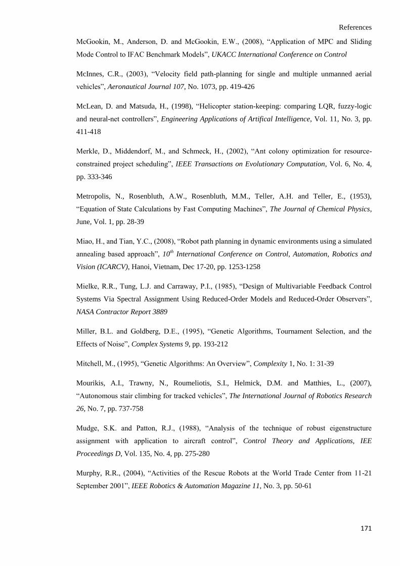
References
171
McGookin, M., Anderson, D. and McGookin, E.W., (2008), “Application of MPC and Sliding
Mode Control to IFAC Benchmark Models”, UKACC International Conference on Control
McInnes, C.R., (2003), “Velocity field path-planning for single and multiple unmanned aerial
vehicles”, Aeronautical Journal 107, No. 1073, pp. 419-426
McLean, D. and Matsuda, H., (1998), “Helicopter station-keeping: comparing LQR, fuzzy-logic
and neural-net controllers”, Engineering Applications of Artifical Intelligence, Vol. 11, No. 3, pp.
411-418
Merkle, D., Middendorf, M., and Schmeck, H., (2002), “Ant colony optimization for resource-
constrained project scheduling”, IEEE Transactions on Evolutionary Computation, Vol. 6, No. 4,
pp. 333-346
Metropolis, N., Rosenbluth, A.W., Rosenbluth, M.M., Teller, A.H. and Teller, E., (1953),
“Equation of State Calculations by Fast Computing Machines”, The Journal of Chemical Physics,
June, Vol. 1, pp. 28-39
Miao, H., and Tian, Y.C., (2008), “Robot path planning in dynamic environments using a simulated
annealing based approach”, 10th International Conference on Control, Automation, Robotics and
Vision (ICARCV), Hanoi, Vietnam, Dec 17-20, pp. 1253-1258
Mielke, R.R., Tung, L.J. and Carraway, P.I., (1985), “Design of Multivariable Feedback Control
Systems Via Spectral Assignment Using Reduced-Order Models and Reduced-Order Observers”,
NASA Contractor Report 3889
Miller, B.L. and Goldberg, D.E., (1995), “Genetic Algorithms, Tournament Selection, and the
Effects of Noise”, Complex Systems 9, pp. 193-212
Mitchell, M., (1995), “Genetic Algorithms: An Overview”, Complexity 1, No. 1: 31-39
Mourikis, A.I., Trawny, N., Roumeliotis, S.I., Helmick, D.M. and Matthies, L., (2007),
“Autonomous stair climbing for tracked vehicles”, The International Journal of Robotics Research
26, No. 7, pp. 737-758
Mudge, S.K. and Patton, R.J., (1988), “Analysis of the technique of robust eigenstructure
assignment with application to aircraft control”, Control Theory and Applications, IEE
Proceedings D, Vol. 135, No. 4, pp. 275-280
Murphy, R.R., (2004), “Activities of the Rescue Robots at the World Trade Center from 11-21
September 2001”, IEEE Robotics & Automation Magazine 11, No. 3, pp. 50-61

References
172
Murphy, R.R., Tadokoro, S., Nardi, D., Jacoff, A., Fiorini, P., Choset, H. and Erkmen, A, (2008),
“Search and Rescue Robotics”, in Springer Handbook of Robotics, pp. 1151-1173, Springer Berlin
Heidelberg
Murray-Smith, D.J., (1995), Continuous System Simulation, Chapman & Hall
NHS, 2013, http://www.nhs.uk/Conditions/Hypothermia/Pages/Symptoms.aspx, Symptoms of
hypothermia, 20/9/2013
Nicolaou, S., (1996), Flying Boats and Seaplanes: A history from 1905, Bay View Books Ltd 1998
Niu, B., Fan Y., Tan, L., Rao, J. and Li, L., (2010), “A Review of Bacterial Foraging Optimization
Part I: Background and Development”, Advanced Intelligent Computing Theories and Applications,
pp. 535-543, Springer Berlin Heidelberg
Ogata, K., (2002), Modern Control Engineering, 4th edition, Prentice Hall, New Jersey
Okada, Y., Nagatani, K., Yoshida, K., Tadokoro, S., Yoshida, T. and Koyanagi, E., (2011), “Shared
autonomy system for tracked vehicles on rough terrain based on continuous three-dimensional
terrain scanning”, Journal of Field Robotics 28, No. 6, pp. 875-893
Padfield, G.G., (2007), Helicopter Flight Dynamics: The Theory and Application of Flying
Qualities and Simulation Modelling, 2nd
edition, Blackwell Publishing, Oxford
Park, M.G. and Lee, M.C., (2003), “Artificial Potential Field Based Path Planning for Mobile
Robots Using a Virtual Obstacle Concept”, Proceedings of the IEEE/ASME International
Conference on Advanced Intelligent Mechatronics, Vol. 2, pp. 735-740
Parsopoulos, K.E. and Vrahatis, M.N., (2002), “Particle Swarm Optimization Methods for
Constrained Optimization Problems”, Intelligent Technologies—Theory and Application: New
Trends in Intelligent Technologies 76, pp. 214-220
Parunak, H.V.D., Purcell, M. and O’Connell, R., (2002), “Digital pheromones for autonomous
coordination of swarming UAV’s”, Ann Arbor 1001, 48105-1579
Passino, K.M., (2002), “Biomimicry of bacterial foraging for distributed optimization and control”
IEEE Control Systems, Vol. 22, No. 3, pp. 52-67
Philips, C.L. and Harbor, R.D., (1996), Feedback Control Systems, 3rd
edition, International edition,
Prentice Hall International Inc
Qi, J., Zhao, X., Jiang, Z. and Han, J., (2006), “Design and Implement of a Rotorcraft UAV
Testbed”, Proceedings of the 2006 IEEE International Conference on Robotics and Biomimetics,
Kunming, China, Dec 17-20, pp. 109-114

References
173
Rafferty, K.J. and McGookin, E.W., (2012), “A Comparison of PID and Sliding Mode Controllers
for a Remotely Operated Helicopter”, 12th
International Conference on Control, Automation,
Robotics and Vision (ICARCV), Guangzhou, China, Dec 5-7, pp. 984-989
Rafferty, K.J. and McGookin, E.W., (2013), “An Autonomous Air-Sea Rescue System Using
Particle Swarm Optimization”, 2013 International Conference on Connected Vehicles and Expo,
Las Vegas, U.S.A., 2-6 Dec, pp. 459-464
Rayward-Smith, V.J., Osman, I.H., Reeves, C.R. and Smith, G.D., (1996), Modern Heuristic
Search Methods, John Wiley and Sons Ltd, West Sussex, England
Rugh, W.J. and Shamma, J. S., (2000), “Research on gain scheduling”, Automatica, Vol. 36, No.
10, pp. 1401-1425
Russell, S. and Norvig, P., (1995), Artificial Intelligence: A Modern Approach, Prentice Hall, New
Jersey
Rybski, P.E., Larson, A., Veeraraghavan, H., LaPoint, M. and Gini, M., (2007), “Communication
strategies in multi-robot search and retrieval: Experiences with mindart”, Distributed Autonomous
Robotic Systems 6, pp. 317-326
Sakamoto, T., Katayama, H. and Ichikawa, A., (2006), “Attitude Control of a Helicopter Model by
Robust PID Controllers”, Proceedings of the 2006 IEEE International Symposium on Intelligent
Control, Munich, Germany, Oct 4-6, pp. 1971-1976
Sato, N., Matsuno, F., Yamasaki, T., Kamegawa, T., Shiroma, N. and Igarashi, H., (2004),
“Cooperative task execution by a multiple robot team and its operators in search and rescue
operations”, Proceedings of IEEE/RSJ International Conference on Intelligent Robots and Systems,
Vol. 2, pp. 1083-1088
Schmitt, L., (2004), “Theory of Genetic Algorithms II: models for genetic operators over the string-
tensor representation of populations and convergence to global optima for arbitrary fitness function
under scaling”, Theoretical Computer Science 310, No. 1, pp. 181-231
Schoonderwoerd, R., Holland, O., Bruten, J. and Rothkrantz, L., (1996), “Ant-based load balancing
in telecommunication networks”, Adaptive Behaviour, Vol. 5, No. 2, pp. 169-207
Seshagiri, S. and Khalil, H.K., (2002), “On introducing integral action in sliding mode control”,
Proceedings of the 41st IEEE Conference on Decision and Control, Vol. 2, pp. 1473-1478
Sharma, S.K., Naeem, W. and Sutton, R., (2012), “An Autopilot Based on a Local Control
Network Design for an Unmanned Surface Vehicle”, Journal of Navigation, Vol. 65, No. 2, pp.
281-301

References
174
Sharman, K.C., (1988), “Maximum likelihood parameter estimation by Simulated Annealing”,
Proceedings of the IEEE International Conference on Acoustics, Speech and Signal Processing, pp.
2741-2744
Shi, Y. and Eberhart, R., (1998), “A modified particle swarm optimizer”, IEEE World Congress on
Computational Intelligence, IEEE International Conference on Evolutionary Computation
Proceedings, pp. 69-73
Skogestad, S. and Postlethwaite, I., (2007), Multivariable feedback control: analysis and design,
Vol. 2, Wiley, New York
Slotine, J.J.E. and Li, W., (1991), Applied Nonlinear Control, Prentice Hall
Spurgeon, S.K., Edwards, C. and Foster, N.P., (1996), Robust Model Reference Control Using a
Sliding Mode Controller/Observer Scheme with application to a Helicopter Problem, IEEE
Workshop on Variable Structure Systems, Dec 5-6, pp. 36-41
Stützle, T. and Hoos, H.H., (2000), “MAX-MIN Ant System”, Future Generations Computer
Systems 16, No. 8, pp. 889-914
Suzuki, I. and Żyliński, P., (2008), “Capturing an Evader in a Building – Randomized and
Deterministic Algorithms for Mobile Robots”, IEEE Robotics & Automation Magazine, Vol. 15,
No. 2, pp. 16-26
Tarbouriech, S. and Turner, M., (2009), “Anti-windup design: an overview of some recent
advances and open problems”, IET Control Theory and Applications, Vol. 3, No. 1, pp. 1-19
Tau 640, (2011), “Tau 640 Slow Video Camera User’s Manual”, FLIR Commercial Systems, June
2011
Thomson, D. and Bradley, R., (2006), “Inverse simulation as a tool for flight dynamics research—
Principles and applications”, Progress in Aerospace Sciences 42, No. 3, pp. 174-210
Thomson, D.G. and Bradley, R., (1998), “The principles and practical application of helicopter
inverse simulation”, Simulation Practice and Theory 6, No. 1, pp. 47-70
Tseng, M.L. and Chen, M.S., (2010), “Chattering Reduction of Sliding Mode Control by Low-Pass
Filtering the Control Signal”, Asian Journal of Control, Vol. 12, No. 3, pp. 392-398
University of Minnesota Sea Grant Program, (1983), in Pozos, R. and Wittmers, L., (1983), The
Nature and Treatment of Hypothermia, University of Minnesota
Utkin, V., Guldner, J. and Shi, J., (1999), Sliding Mode Control in Electromechanical Systems,
Taylor & Francis Ltd, London

References
175
Vecchio, C., (2008), Sliding Mode Control: theoretical developments and applications to uncertain
mechanical systems, Ph.D. Thesis, University of Pavia
Visioli, A., (2003), “Modified anti-windup scheme for PID controllers”, IEE Proceedings –
Control Theory and Applications, Vol. 150, No. 1, pp. 49-54
Wang, Q.G., Ye, Z., Cai, W.J. and Hang, C.C., (2008), PID Control for Multivariable Processes,
Springer, Berlin
Wegner, R. and Anderson, J., (2006), “Agent-based support for balancing teleoperation and
autonomy in urban search and rescue”, International Journal of Robotics and Automation 21, No. 2,
pp. 120-128
Wei, J.D. and Lee, D.T., (2004), “A New Approach to the Travelling Salesman Problem Using
Genetic Algorithms with Priority Encoding”, Congress on Evolutionary Computation, Vol. 2, pp.
1457-1464
Wilhelm, M.R. and Ward, T.L., (1987), “Solving Quadratic Assignment Problems by ‘Simulated
Annealing’ ”, IIE transations, Vol. 19, No. 1, pp. 107-119
Wonham, W.M., (1967), “On-Pole Assignment in Multi-Input Controllable Linear Systems”, IEEE
Transactions on Automatic Control, Vol. AC-12, No. 6, pp. 660-665
Worrall, K.J., (2008), Guidance and Search Algorithms for Mobile Robots: Application and
Analysis within the Context of Urban Search and Rescue, Ph.D. Thesis, Department of Electronics
and Electrical Engineering, University of Glasgow
Xi, B., Liu, Z., Raghavachari, M., Xia, C.H. and Zhang, L., (2004), “A Smart Hill-Climbing
Algorithm for Application Server Configuration”, Proceedings of the 13th international conference
on World Wide Web, pp. 287-296
Xiao, Q., Zou, D. and Wei, P., (2010), “Fuzzy Adaptive PID Control Tank Level”, International
Conference on Multimedia Communications, Hong Kong, Aug 7-8, pp. 149-152
Xiaofeng, G., Jinchang, G. and Chunhui, Z., (1996), “Extension of IMC Tuning to Improve
Controller Performance”, IEEE International Conference on Systems, Man, and Cybernatics, Oct
14-17, Vol. 3, pp. 1770-1775
Yaman, F., and Yilmaz, A.E., (2010), “Investigation of fixed and variable mutation rate
performance in real coded Genetic Algorithm for uniform circular antenna array pattern synthesis
problem”, IEEE 18th Signal Processing and Communications Applications Conference, pp. 594-
597

References
176
Yim, M. and Laucharoen, J., (2011), “Towards small robot aided victim manipulation”, Journal of
Intelligent & Robotic Systems 64, No. 1, pp. 119-139
Yoshida, H., Fukuyama, Y., Takayama, S., and Nakanishi, Y., (1999), “A particle swarm
optimization for reactive power and voltage control in electric power systems considering voltage
security assessment”, Proceedings of the IEEE International Conference on Systems, Man and
Cybernatics, Tokyo, Oct 12-15, Vol. 6, pp. 497-502
Young, H.D. and Freedman, R.A., (2004), University Physics with Modern Physics, 11th edition,
Pearson Education, Addison Wesley, United States of America
Young, K.D., Utkin, V.I., and Ӧzgüner, U., (1999), “A Control Engineer’s Guide to Sliding Mode
Control”, IEEE Transactions on Control Systems Technology, Vol. 7, No. 3, pp. 328-342
Zengin, U. and Dogan, A., (2007), “Real-Time Target Tracking for Autonomous UAVs in
Adversarial Environments: A Gradient Search Algorithm”, IEEE Transactions on Robotics, Vol.
23, No. 2, pp. 294-307
Zhang, B., Chen, W. and Fei, M., (2006), “An optimized method for path planning based on
artificial potential field”, Sixth International Conference on Intelligent Systems Design and
Applications, IEEE, Vol. 3, pp. 35-39
Zhang, X., Wu, M., Peng, J. and Jiang, F., (2009) “A Rescue Robot Path Planning Based on Ant
Colony Optimization Algorithm”, International Conference on Information Technology and
Computer Science, Kiev, Ukraine, 25-26 Jul, pp. 180-183
Zhang, Z., Nejat, G., Guo, H. and Huang, P., (2011), “A novel 3D sensory system for robot-
assisted mapping of cluttered urban search and rescue environments”, Intelligent Service Robotics
4, No. 2, pp. 119-134
Zhao, Z.Y., Tomizuka, M. and Isaka, S., (1993), “Fuzzy Gain Scheduling of PID Controllers”,
IEEE Transactions on Systems, Man and Cybernatics, Vol. 23, No. 5, pp. 1392-1398
Zhuang, M. and Atherton, D.P., (1993), “Automatic tuning of optimum PID controllers”, Control
Theory and Applications, IEE Proceedings D, Vol. 140, No. 3, pp. 216-224
Ziegler, J.G. and Nichols, N.B., (1942), “Optimum Settings for Automatic Controllers”, Trans.
ASME, 1942, Vol. 64, pp. 759-768

Appendix A
177
Appendix A: Rotational Transformation
This appendix derives the full rotational transformation matrix from the Earth-fixed axes to the
body-fixed axes of the helicopter, which are obtained from the Earth-fixed axes by three successive
rotations: a rotation about the Earth-fixed z-axis (in the positive direction) by the yaw angle ψ, a
rotation about the new y-axis by the pitch angle θ, and finally, a rotation about the new x-axis by
the roll angle ϕ. The full transformation matrix is derived by considering these three rotations
individually.
First of all, consider the rotation about the Earth-fixed z-axis by the heading angle ψ: the z
coordinate will stay the same but the x and y coordinates will change, as illustrated below, where x
changes to x1 and y changes to y1:
Figure A.1: Heading Transformation
Note that using the right-hand coordinate system, the z-axis points out of the page, so an anti-
clockwise rotation corresponds to a positive ψ, and a clockwise rotation corresponds to a negative
ψ. The position vector (x,y) can be written as a complex number x+iy. Now, the x and y
coordinates of the same point in the new coordinate system (which is a rotation of the old
coordinate system by ψ) is the same as if the coordinate system remained the same, but the actual
point was rotated by the same angle in the opposite direction, which corresponds to a rotation of –ψ.
Using complex numbers, this is the same as multiplying the original position vector by
ψψψ isincose i . Therefore, the new position vector is given by
ψψψψψψ ycosxsiniysinxcosisincosiyxiyx 11 (A.1)
and hence, the rotation of ψ about the z-axis transforms the original coordinates (x, y, z) to the new
coordinates (x1, y1, z1), where
y
y1
x
x1
y1
y
x1 ψ
ψ
x

Appendix A
178
ψψ ysinxcosx1
ψψ ycosxsiny1
zz1
This can be written as the following matrix equation
z
y
x
100
0 cossin
0sin cos
z
y
x
1
1
1
ψψ
ψψ
Thus, the rotation about the z-axis by the heading angle ψ transforms the original Earth-fixed frame
to a new frame by the following transformation matrix:
100
0cossin
0sincos
R ψψ
ψψ
ψ (A.2)
The second rotation is about the new y-axis (the y1-axis) by the pitch angle θ, which transforms x1
and z1 to x2 and z2 respectively, with the y-coordinate staying the same, as illustrated below:
Figure A.2: Pitch Transformation
Again, note that this orientation is consistent with the y1 axis pointing out of the page, so that an
anti-clockwise rotation corresponds to a positive θ, and a clockwise rotation corresponds to a
negative θ. Using a similar analysis to the first transformation, it can be shown that this rotation
transforms the coordinates (x1, y1, z1) to the new coordinates (x2, y2, z2), where
θθ sinzcosxx 112
12 yy
x1
x2 z1
x1 z2
x2
z2 θ
θ
z1
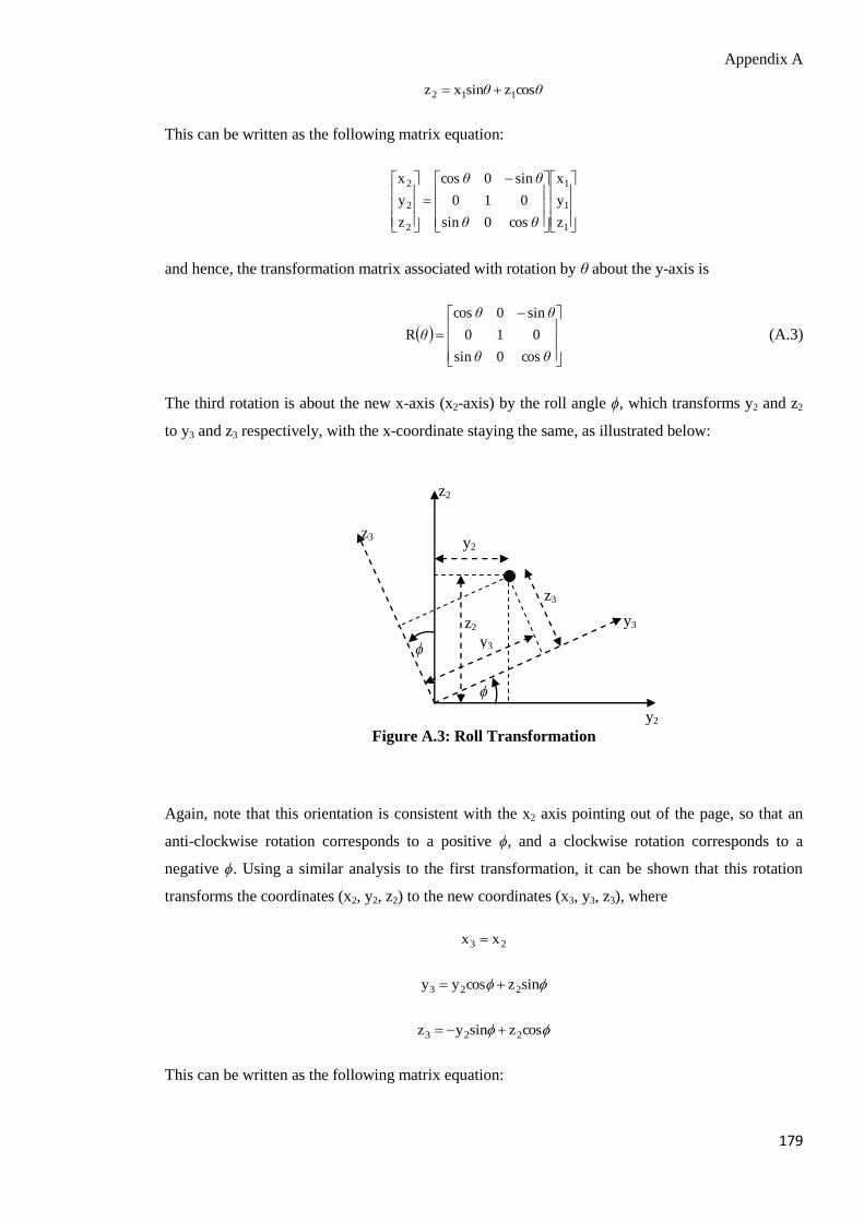
Appendix A
179
θθ coszsinxz 112
This can be written as the following matrix equation:
1
1
1
2
2
2
z
y
x
cos0sin
010
sin 0 cos
z
y
x
θθ
θθ
and hence, the transformation matrix associated with rotation by θ about the y-axis is
θθ
θθ
θ
cos0sin
010
sin 0 cos
R (A.3)
The third rotation is about the new x-axis (x2-axis) by the roll angle ϕ, which transforms y2 and z2
to y3 and z3 respectively, with the x-coordinate staying the same, as illustrated below:
Figure A.3: Roll Transformation
Again, note that this orientation is consistent with the x2 axis pointing out of the page, so that an
anti-clockwise rotation corresponds to a positive ϕ, and a clockwise rotation corresponds to a
negative ϕ. Using a similar analysis to the first transformation, it can be shown that this rotation
transforms the coordinates (x2, y2, z2) to the new coordinates (x3, y3, z3), where
23 xx
sinzcosyy 223
coszsinyz 223
This can be written as the following matrix equation:
z2
y2
z3
z2 y3
z3
y3 ϕ
ϕ
y2

Appendix A
180
2
2
2
3
3
3
z
y
x
cossin0
sincos0
001
z
y
x
and hence, the transformation matrix associated with rotation by ϕ about the x-axis is
cossin0
sincos0
001
R (A.4)
Thus, the complete transformation from the Earth-fixed axes to the body-fixed axes can be
described by the product of these transformation matrices, which is given by
coscoscossinsinsincossinsincossincos
cossincoscossinsinsinsincoscossinsin
sinsincoscoscos
,,R (A.5)

Appendix B
181
Appendix B: Helicopter Model
This appendix presents the model of the X-Cell 60 SE helicopter in more detail. In particular, the
details of the individual forces and moments that act on the helicopter are presented, and the model
for the engine, governor and rotor speed is discussed. The corresponding equations can be found in
Gavrilets (2003). Finally, the matrices that form the linearized model of the helicopter are
presented; these matrices were calculated numerically on Matlab.
B1 Forces and Moments
The forces and moments that are included in the equations of motion can be broken down as shown
below:
X = Xmr + Xfus (B1.1)
Y = Ymr + Yfus +Ytr + Yvf (B1.2)
Z = Zmr + Zfus + Zht (B1.3)
L = Lmr + Lvf + Ltr (B1.4)
M = Mmr + Mht (B1.5)
N = –Qe + Nvf + Ntr (B1.6)
The subscripts represent the different parts of the helicopter, as defined below:
‘mr’ – main rotor
‘fus’ – fuselage
‘tr’ – tail rotor
‘vf’ – vertical fin
‘ht’ – horizontal tail/stabilizer
‘e’ – engine

Appendix B
182
The actual expressions for the forces and moments are rather complicated, and require many more
definitions. The inflow ratio λ0 and thrust coefficient CT for the main rotor are related by the
following equations:
2z0
2w
T0
μλμ2η
Cλ
(B1.7)
2
λμ
2
μ
3
1θ
2
σaC 0z
2
0mrmrideal
T (B1.8)
C C if C
C C if C
CCC if C
CidealT
maxT
maxT
maxT
idealT
maxT
maxT
idealT
maxT
idealT
T (B1.9)
22
maxmaxT
πRΩRρ
TC (B1.10)
The various terms in equations (B1.7) – (B1.10) (that have not been defined already) are as
follows: ηw is a coefficient which represents non-ideal wake contraction due to a non-uniform
wake; μ is the advance ratio; μz is the normal airflow component; amr is the lift curve slope for the
main rotor; σmr is the main rotor solidity ratio; θ0 is the collective pitch angle of the main rotor
blades; maxTC is the maximum main rotor thrust coefficient; Tmax is the maximum main rotor
thrust; ρ is the air density; R is the main rotor radius.
These equations can be solved iteratively to find the inflow ratio λ0 and thrust coefficient CT for the
main rotor. The main rotor thrust can then be calculated using the equation
Tmr = CTρ(ΩR)2πR
2 (B1.11)
The main rotor torque is assumed to be a combination of the torque due to the thrust, and the torque
due to profile drag on the blades; the torque coefficient, CQ, can therefore be determined from the
following equation:
2D
z0TQ μ3
71
8
σCμλCC 0 (B1.12)
where 0DC is the main rotor blade zero lift drag coefficient. Consequently the main rotor torque is
32Qmr πRΩRρCQ (B1.13)
The main rotor rolling and pitching moments are assumed to consist of the moments due to the
tilting of the thrust vector, and the restraint in the blades, which can be approximated as the
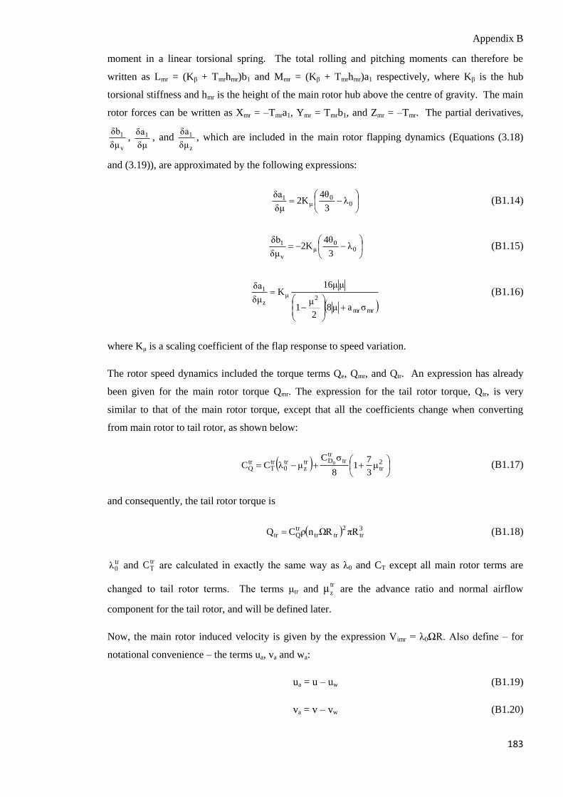
Appendix B
183
moment in a linear torsional spring. The total rolling and pitching moments can therefore be
written as Lmr = (Kβ + Tmrhmr)b1 and Mmr = (Kβ + Tmrhmr)a1 respectively, where Kβ is the hub
torsional stiffness and hmr is the height of the main rotor hub above the centre of gravity. The main
rotor forces can be written as Xmr = –Tmra1, Ymr = Tmrb1, and Zmr = –Tmr. The partial derivatives,
v
1
δμ
δb, δμ
δa1 , and z
1
δμ
δa, which are included in the main rotor flapping dynamics (Equations (3.18)
and (3.19)), are approximated by the following expressions:
0
0μ
1 λ3
4θ2K
δμ
δa (B1.14)
0
0μ
v
1 λ3
4θ2K
δμ
δb (B1.15)
mrmr
2μz
1
σaμ82
μ1
μ16μK
δμ
δa
(B1.16)
where Kμ is a scaling coefficient of the flap response to speed variation.
The rotor speed dynamics included the torque terms Qe, Qmr, and Qtr. An expression has already
been given for the main rotor torque Qmr. The expression for the tail rotor torque, Qtr, is very
similar to that of the main rotor torque, except that all the coefficients change when converting
from main rotor to tail rotor, as shown below:
2
tr
trtrDtr
ztr0
trT
trQ μ
3
71
8
σCμλCC 0 (B1.17)
and consequently, the tail rotor torque is
3tr
2trtr
trQtr πRΩRnρCQ (B1.18)
tr0λ and
trTC are calculated in exactly the same way as λ0 and CT except all main rotor terms are
changed to tail rotor terms. The terms μtr and tr
zμ are the advance ratio and normal airflow
component for the tail rotor, and will be defined later.
Now, the main rotor induced velocity is given by the expression Vimr = λ0ΩR. Also define – for
notational convenience – the terms ua, va and wa:
ua = u – uw (B1.19)
va = v – vw (B1.20)

Appendix B
184
wa = w – ww (B1.21)
In other words, these are simply the velocity components relative to the wind. Now, define the term
2imra2a
2a VwvuV . The fuselage forces along the body axes can then be approximated as
VuS 0.5ρX afusxfus (B1.22)
VvS 0.5ρY afusyfus (B1.23)
VVwS 0.5ρZ imrafuszfus (B1.24)
which are effectively drag forces. The terms fusxS , fus
yS and fuszS are the effective frontal, side and
vertical drag areas respectively. Now, the side and vertical velocity (relative to the wind) at the
vertical fin (same as for the tail rotor) can be written as
rlVεvv tritrtrvfavf (B1.25)
imrλtratr VKqlww (B1.26)
Vitr is the induced velocity of the tail rotor, which can be calculated in exactly the same way as the
main rotor induced velocity, except the main rotor terms should be replaced by the corresponding
tail rotor terms. The wake intensity factor Kλ will be defined shortly. The trvfε term is the fraction
of the vertical fin area exposed to the tail rotor induced velocity, and ltr is the location of the tail
rotor hub behind the centre of gravity. Now, define 2tr
2a
tr wuV . Then the vertical fin side
force can be approximated as
vfvftrvf
Lvfvf vvVCS 0.5ρYα
(B1.27)
which is a combination of lift and drag. The vfLα
C term is the vertical fin lift curve slope. With the
vertical fin side force defined, the rolling and yawing moment from the vertical fin can be defined,
as shown below:
trvfvf hYL (B1.28)
trvfvf lYN (B1.29)
where, htr is the height of the tail rotor hub above the centre of gravity.
The forces and moments from the horizontal stabilizer will now be discussed. The effective
vertical velocity at the horizontal stabilizer is given by

Appendix B
185
imrλhtaht VKqlww (B1.30)
where lht is the stabilizer (horizontal tail) location behind the centre of gravity. The vertical (lift and
drag) force at the horizontal stabilizer is then
hthtahtLhtht wwuCS 0.5ρZα
(B1.31)
where htLα
C is the horizontal tail lift curve slope and Sht is the horizontal fin area. The pitching
moment created by this force is
hththt lZM (B1.32)
Finally, the forces and moments from the tail rotor are discussed. First of all, some of the terms
introduced earlier are defined: expressions are required for the terms Kλ, μtr and trzμ . The side
velocity at the tail rotor is given by phrlvv trtratr . The terms μtr and tr
zμ are then given by
trtr
2tr
2a
trΩRn
wuμ
(B1.33)
and
trtr
trtrz
ΩRn
vμ (B1.34)
The wake intensity factor Kλ depends on the tangents of certain angles. Define
tr
trmrtri
h
RRlg
(B1.35)
and
tr
trmrtrf
h
RRlg
(B1.36)
Then if aimr wV or iaimr
a gwV
u
, the tail rotor is out of the wake, because in the first case, the
downward velocity is too large for the wake to catch up with the tail rotor, and in the second case,
the helicopter is moving too slowly in the forward direction for the tail rotor to catch up with the
wake. In both cases, Kλ = 0. If faimr
a gwV
u
, then the tail rotor is fully in the wake, and it is
assumed that Kλ = 1.5. When the tail rotor is partially in the wake, i.e. when faimr
ai g
wV
ug
, it
is assumed that Kλ grows linearly, as shown by the following equation:

Appendix B
186
if
iaimr
a
λgg
gwV
u
1.5K
(B1.37)
This gives the necessary definitions for some of the forces and moments calculated earlier.
Now, the side force produced by the tail rotor can be written as
2tr
2trtr
trTttr πRΩRnρCfY (B1.38)
where the term ft is a fin blockage factor, and is given by
2tr
vft
πR
S
4
31f (B1.39)
and Svf is the effective vertical fin area. Thus, the rolling and yawing moments produced by the tail
rotor are
trtrtr hYL (B1.40)
trtrtr lYN (B1.41)
This completes the discussion of the individual forces and moments that act on the helicopter.
B2 Rotor Speed Model
Recall from Equation (3.20) that the rotor speed dynamic are given by
trtrmrerot
QnQQI
1rΩ
where Ω is the main rotor speed, r is the yaw rate, Irot is the total rotating inertia referenced to the
main rotor speed, Qe is the torque produced by the engine, Qmr is the main rotor torque, Qtr is the
tail rotor torque and ntr is the gear ratio of the tail rotor to the main rotor. The throttle setting, which
is denoted δt, affects the engine torque, which subsequently affects the rotor speed. When a desired
rotor speed is commanded, the throttle changes automatically so that the rotor speed reaches this
desired value, and in order to simulate the system, this model must be identified. There were no
look-up tables available to determine the relationship between the throttle setting and the engine
torque, so a simplified model was used to represent this. Gavrilets (2003) used the following
representation:
tmaxee δPP (B2.1)

Appendix B
187
where Pe is the engine power, Pemax
is the maximum engine power, and δt is the throttle setting,
which takes on a value between 0 and 1. The engine torque is then represented by the following
equation:
Ω
PQ e
e (B2.2)
This establishes the relationship between the throttle and the engine torque, so a relationship must
now be established between the desired rotor speed and the throttle. This is modelled as a PI
controller with proportional and integral gains KP and KI. The throttle can therefore be represented
by the following equation:
t
0
cIcPt dτΩΩKΩΩKδ (B2.3)
where Ωc is the commanded rotor speed. The gains were then calculated by Gavrilets (2003) by
performing time-frequency analysis on the sound of the engine when a step input in rotor speed
was commanded. After analysing the data, the proportional and integral gains were determined to
be 0.01 and 0.02 respectively. This model is then used to represent the rotor speed dynamics.
B3 Linearized Model
From Section 3.5, the helicopter mathematical model can be written in the form
uxx BA
where x is the state vector, u is the control vector, A is the system matrix, and B is the control
matrix. In this case, the state vector is given by
x = [pn , pe , pd , u , v , w , ϕ , θ , ψ , p , q , r , b1 , a1 , Ω]T
The individual terms represent north, east, and downward positions, surge, sway, and heave
velocities, roll, pitch, and yaw angles, roll, pitch, and yaw rates, lateral and longitudinal flapping
angles of main rotor blades, and angular velocity of main rotor blades respectively. The control
vector is given by
Tt0tr0lonlat δ,θ,θ,δ,δu
The individual terms represent lateral and longitudinal cyclic inputs, main rotor and tail rotor
collective pitch angles, and throttle setting respectively.

Appendix B
188
The following matrices represent the linearized model at hover:
0.87000.9700.080000.141.060000
08.35001.000000000000
008.35001.00000000000
0.45000.9900.0800001.080000
0213.010000000000000
0.030402.360.1300.010000.070.150000
0001.000.090000000000
0000.091.000000000000
000001.00000000000
0.1200000000.860.9400000
0.0109.560.0400009.770.010.110000
09.56000009.810000.03000
0000000001.000.090000
0000000000.091.000000
000000000001.00000
A
83.2993.36450.1400
00035.070
000035.07
42.77135.88000
00000
018.5812.1500
00000
00000
00000
00136.6600
05.101.1400
00000
00000
00000
00000
B

Appendix B
189
The following matrices represent the linearized model at a forward speed of 5m/s:
0.82001.310.190.090000.431.440.69000
08.35001.000000000000
008.35001.00000000000
0.39001.320.200.090000.061.450.58000
0213.20000.0400000.0300.15000
0.030402.700.180.030.010000.100.200.04000
0001.000.080000000000
0000.081.000000000000
0000.0201.00000000000
0.100005.00000.200.781.2800.53000
009.594.950.01000.029.780.010.150.02000
09.59000009.8100.0300.07000
00000005.0001.000.080.02000
0000005.00000.081.000000
00000000.1000.0201.00000
A
83.2991.29374.6300
000.1435.070
000035.07
42.77129.230.2000
001.7100
017.6710.6200
00000
00000
00000
00130.7200
04.851.1000
000.3700
00000
00000
00000
B

Appendix B
190
The following matrices represent the linearized model at a forward speed of 10m/s:
0.75001.870.160.120001.692.050.77000
08.35001.000000000000
008.35001.00000000000
0.33001.830.160.120000.092.020.61000
0.01213.32000.3200000.2800.02000
0.020402.950.250.020.020000.130.280.06000
0001.000.070000000000
0000.071.000000000000
0000.070.011.00000000000
0.100009.98000.700.691.7700.31000
0.0109.629.930.01000.059.760.010.240.02000
09.62000009.7800.0100.15000
00000009.9700.990.070.07000
0000009.97000.071.000000
00000000.7200.070.011.00000
A
83.2994.38265.2500
000.2935.070
000035.07
42.77124.657.2900
0013.9200
017.059.5600
00000
00000
00000
00145.7900
04.680.7100
000.4200
00000
00000
00000
B

Appendix C
191
Appendix C: Individual Results
This appendix presents the individual results of all the simulations carried out in Chapters 6, 7 and
8. For each method, 100 simulations were run and each table presents the number of targets
detected for each run, the percentage coverage for each run, and the time taken to detect the first
target for each run. The mean, median, and standard deviation values of each of these terms are
also given. Note that in the cases where no targets are detected, in order to calculate an appropriate
mean for the time of the first detection, a time of 540s is used as this is the total time of each
simulation. In each table, the highlighted row indicates the simulation presented in the main part of
the thesis. Section C1 presents the results for the standard search patterns (Parallel Sweep, Sector
Search, and Expanding Square), Section C2 presents the results for the optimisation techniques that
don’t include the probability distribution (which are tested in Chapter 6), Section C3 presents the
results for the optimisation techniques that do include the probability distribution (which are tested
in Chapter 7), and finally, Section C4 presents the results for the hybrid optimisation techniques,
which are tested in Chapter 8.
C1 Standard Search Patterns: Individual Results
This section presents the individual results for the standard search patterns. These results are
discussed in Section 6.3.

Appendix C
192
Table C1.1: Parallel Sweep
Run
Number
Targets
Detected
%
Coverage
Time of First
Detection (s)
Run
Number
Targets
Detected
%
Coverage
Time of First
Detection (s)
1 4 46.68 109.24 51 5 46.51 73.60
2 6 46.42 117.32 52 7 46.50 47.08
3 4 46.34 98.44 53 4 46.41 37.28
4 4 46.41 76.64 54 7 46.45 38.20
5 7 46.42 25.00 55 6 46.46 112.72
6 6 46.34 269.08 56 6 46.40 126.56
7 6 46.43 168.32 57 7 46.94 41.64
8 6 46.47 25.00 58 5 46.44 174.60
9 4 46.43 77.12 59 3 46.38 170.60
10 6 46.89 89.48 60 6 46.68 168.80
11 5 46.43 50.40 61 5 46.40 99.76
12 3 46.58 42.84 62 8 46.46 25.00
13 3 46.44 99.32 63 4 46.38 172.68
14 7 46.47 53.80 64 8 46.47 54.48
15 3 46.60 36.68 65 8 46.84 43.32
16 4 46.40 113.92 66 4 46.42 171.60
17 7 46.49 43.28 67 2 46.45 89.92
18 4 46.72 81.84 68 4 46.53 25.00
19 7 46.46 124.52 69 5 46.43 45.32
20 5 46.52 43.60 70 5 46.39 101.36
21 4 46.41 36.16 71 5 46.35 38.08
22 3 46.47 34.88 72 6 46.50 58.52
23 6 46.44 43.00 73 6 46.43 25.00
24 5 46.49 119.44 74 7 46.40 171.36
25 4 46.47 43.40 75 7 46.53 68.68
26 6 46.42 57.44 76 7 46.72 165.68
27 7 46.46 225.16 77 7 46.43 161.64
28 7 46.46 25.00 78 6 46.40 98.60
29 7 46.54 33.44 79 6 46.37 112.52
30 2 46.32 98.24 80 3 46.48 37.36
31 8 46.49 52.88 81 8 46.44 50.32
32 3 46.48 114.72 82 7 46.97 55.00
33 2 46.47 140.76 83 5 46.50 30.92
34 6 46.49 118.28 84 7 46.52 64.08
35 3 46.48 82.56 85 4 46.52 179.72
36 8 46.41 25.00 86 8 46.43 249.00
37 8 46.39 33.32 87 6 46.38 25.00
38 6 46.38 31.52 88 1 46.39 251.92
39 8 46.52 59.92 89 6 46.39 49.52
40 5 46.70 77.88 90 6 46.80 60.60
41 7 46.50 73.68 91 8 46.81 61.60
42 7 46.36 42.12 92 6 46.47 55.32
43 5 46.44 59.84 93 7 46.39 25.00
44 4 46.22 59.24 94 5 46.50 53.20
45 7 46.49 77.16 95 7 46.35 156.80
46 9 46.43 25.00 96 5 46.41 53.20
47 6 46.47 223.28 97 6 46.39 85.24
48 8 46.43 41.16 98 7 46.47 167.92
49 2 46.40 126.56 99 7 46.23 45.68
50 1 46.45 187.64 100 8 46.44 59.00
Mean 5.58 46.48 86.51
Median 6 46.45 61.10
St. Dev. 1.79 0.13 58.64

Appendix C
193
Table C1.2: Sector Search
Run
Number
Targets
Detected
%
Coverage
Time of First
Detection (s)
Run
Number
Targets
Detected
%
Coverage
Time of First
Detection (s)
1 7 43.35 136.16 51 6 43.29 137.96
2 5 43.39 78.88 52 5 43.47 57.80
3 4 43.35 54.20 53 5 43.32 121.16
4 0 43.42 N/A 54 8 43.26 57.60
5 5 43.31 25.00 55 1 43.22 228.60
6 5 43.32 110.36 56 4 43.31 48.20
7 7 43.35 80.80 57 9 43.41 34.36
8 8 43.32 25.00 58 6 43.30 37.96
9 3 43.33 112.20 59 6 43.25 225.40
10 4 43.35 33.40 60 5 43.39 100.36
11 5 43.22 49.24 61 6 43.32 50.40
12 5 43.34 43.16 62 7 43.28 25.00
13 3 43.25 77.80 63 5 43.27 98.60
14 8 43.22 70.00 64 5 43.34 54.48
15 4 43.40 35.24 65 6 43.27 29.96
16 4 43.35 60.92 66 7 43.27 94.08
17 7 43.43 36.92 67 5 43.32 39.12
18 7 43.38 42.16 68 4 43.32 25.00
19 3 43.39 65.84 69 5 43.52 65.52
20 6 43.21 48.60 70 8 43.40 31.80
21 6 43.21 37.64 71 8 43.23 93.12
22 6 43.31 34.72 72 3 43.33 58.40
23 8 43.38 39.68 73 7 43.28 25.00
24 3 43.35 85.56 74 5 43.29 159.88
25 6 43.33 91.52 75 4 43.20 103.28
26 3 43.37 57.16 76 2 43.23 336.32
27 4 43.24 68.28 77 6 43.22 70.72
28 7 43.31 25.00 78 3 43.31 49.32
29 5 43.30 43.64 79 6 43.27 77.84
30 5 43.36 156.00 80 5 43.25 38.72
31 5 43.26 78.96 81 4 43.25 45.96
32 3 43.32 78.08 82 5 43.25 54.92
33 6 43.44 203.24 83 6 43.28 30.68
34 3 43.32 272.40 84 5 43.31 148.36
35 7 43.32 36.92 85 3 43.31 77.00
36 7 43.37 25.00 86 8 43.30 71.36
37 8 43.32 53.52 87 6 43.37 25.00
38 5 43.31 104.52 88 7 43.33 157.08
39 7 43.37 59.88 89 4 43.30 69.16
40 6 43.42 87.92 90 5 43.30 60.88
41 2 43.28 136.84 91 6 43.34 62.12
42 6 43.23 180.88 92 7 43.31 55.24
43 4 43.35 59.88 93 6 43.42 25.00
44 3 43.31 59.04 94 2 43.46 53.12
45 5 43.26 106.52 95 6 43.35 94.24
46 8 43.34 25.00 96 3 43.29 79.60
47 5 43.23 103.80 97 8 43.29 93.52
48 5 43.37 39.36 98 5 43.34 117.28
49 5 43.50 135.24 99 6 43.27 44.56
50 4 43.29 76.36 100 6 43.38 59.00
Mean 5.27 43.32 82.88
Median 5 43.32 60.90
St. Dev. 1.74 0.06 71.60

Appendix C
194
Table C1.3: Expanding Square
Run
Number
Targets
Detected
%
Coverage
Time of First
Detection (s)
Run
Number
Targets
Detected
%
Coverage
Time of First
Detection (s)
1 2 47.32 184.80 51 7 47.51 242.20
2 6 47.55 66.04 52 6 47.27 61.76
3 4 47.55 57.28 53 6 47.23 167.60
4 5 47.66 247.00 54 6 47.54 351.72
5 5 47.33 25.00 55 7 47.65 63.08
6 6 47.39 83.56 56 9 47.57 302.28
7 4 47.58 85.92 57 6 47.61 43.20
8 8 47.33 25.00 58 6 47.37 120.80
9 4 47.46 151.68 59 4 47.44 77.96
10 5 47.45 32.84 60 2 47.38 104.36
11 7 47.46 44.80 61 5 47.66 103.12
12 7 47.34 288.04 62 5 47.59 25.00
13 6 47.53 171.68 63 4 47.36 42.32
14 1 47.56 380.24 64 2 47.47 248.00
15 6 47.29 35.68 65 3 47.46 29.60
16 7 47.64 60.72 66 5 47.53 42.60
17 4 47.44 62.44 67 3 47.53 39.04
18 9 47.36 39.20 68 8 47.14 25.00
19 5 47.31 74.44 69 4 47.40 65.92
20 9 47.64 45.72 70 6 47.45 31.20
21 6 47.61 33.88 71 5 47.46 87.08
22 7 47.49 352.92 72 4 47.44 56.48
23 7 47.22 40.20 73 8 47.44 25.00
24 4 47.35 188.76 74 7 47.49 74.40
25 7 47.39 86.20 75 8 47.47 277.08
26 6 47.35 63.56 76 6 47.24 62.12
27 4 47.64 257.44 77 6 47.28 72.44
28 6 47.26 25.00 78 5 47.41 200.40
29 9 47.16 34.48 79 6 46.91 158.04
30 3 47.60 202.20 80 7 47.41 37.16
31 6 47.60 99.72 81 7 47.60 49.40
32 7 47.51 65.88 82 6 47.25 32.72
33 4 47.59 57.12 83 6 47.38 30.52
34 8 47.49 55.16 84 4 47.37 276.76
35 7 47.38 33.16 85 8 47.63 80.88
36 5 47.36 25.00 86 3 47.25 288.80
37 7 47.26 49.56 87 7 47.58 25.00
38 8 47.45 44.40 88 7 47.40 70.92
39 3 47.33 269.84 89 4 47.69 201.36
40 7 47.52 45.68 90 7 47.36 260.72
41 4 47.72 281.44 91 5 47.61 63.08
42 6 47.37 286.32 92 2 47.38 276.64
43 5 47.29 36.36 93 5 47.43 25.00
44 6 47.34 32.68 94 6 47.27 61.92
45 3 47.37 63.04 95 7 47.43 79.04
46 6 47.38 25.00 96 5 47.55 285.44
47 8 47.35 87.56 97 6 47.33 40.48
48 4 47.45 42.32 98 2 47.32 168.64
49 5 47.51 195.12 99 6 47.57 44.48
50 5 47.19 257.48 100 6 47.50 187.48
Mean 5.58 47.43 112.86
Median 6 47.44 64.72
St. Dev. 1.75 0.14 97.19

Appendix C
195
C2 Optimisation Techniques: Individual Results
This section presents the individual results for the optimisation techniques tested in Section 6.4.
Table C2.1: Random Search
Run
Number
Targets
Detected
%
Coverage
Time of First
Detection (s)
Run
Number
Targets
Detected
%
Coverage
Time of First
Detection (s)
1 7 47.36 60.24 51 7 46.02 121.36
2 9 48.33 57.04 52 8 46.29 47.96
3 2 39.46 172.96 53 6 45.48 41.64
4 8 48.38 111.20 54 3 45.49 113.48
5 8 46.61 25.00 55 7 46.35 102.08
6 6 50.67 208.40 56 8 45.47 45.44
7 7 44.92 187.72 57 9 45.64 44.04
8 10 46.01 25.00 58 8 48.23 38.24
9 8 45.16 105.36 59 9 47.50 110.92
10 7 42.36 32.36 60 8 47.76 62.08
11 5 46.53 133.92 61 9 45.69 124.48
12 3 43.03 221.40 62 9 46.25 25.00
13 5 48.32 214.84 63 5 49.68 37.44
14 4 47.48 74.48 64 10 46.41 91.84
15 4 42.92 35.68 65 6 47.31 29.84
16 8 47.81 36.16 66 6 47.02 233.16
17 10 46.82 40.96 67 7 45.77 36.32
18 6 47.94 34.64 68 6 46.94 25.00
19 9 44.50 93.36 69 8 47.05 68.96
20 7 44.89 149.56 70 6 46.57 60.44
21 8 47.29 34.04 71 4 44.45 37.80
22 8 46.93 66.12 72 8 48.50 55.72
23 6 48.61 96.88 73 8 46.18 25.00
24 6 45.25 59.32 74 2 43.69 72.32
25 7 47.93 39.64 75 7 44.98 161.08
26 3 45.53 67.36 76 6 49.62 62.56
27 4 44.92 193.52 77 7 46.44 69.08
28 8 46.82 25.00 78 3 50.82 51.00
29 9 46.78 34.64 79 7 46.84 57.04
30 8 44.68 99.96 80 5 49.33 47.08
31 5 49.30 216.32 81 6 46.72 49.36
32 7 49.74 77.44 82 9 45.37 32.84
33 4 45.87 65.24 83 10 47.82 31.08
34 10 47.24 53.64 84 7 46.66 289.00
35 4 47.29 33.36 85 10 47.35 158.44
36 8 46.62 25.00 86 8 47.44 99.44
37 6 43.45 49.64 87 10 43.94 25.00
38 5 46.41 106.60 88 5 44.72 68.96
39 7 42.76 164.72 89 10 44.02 116.88
40 5 45.23 74.68 90 9 44.59 111.20
41 5 44.23 73.68 91 7 44.40 259.52
42 5 47.96 40.04 92 7 47.63 73.60
43 6 45.58 79.80 93 6 47.24 25.00
44 3 48.46 33.08 94 8 45.02 60.28
45 9 43.27 206.52 95 8 46.59 95.96
46 7 47.37 25.00 96 4 49.57 106.92
47 8 45.22 123.08 97 7 46.93 41.04
48 8 45.99 42.24 98 8 45.77 110.76
49 9 49.20 77.92 99 7 46.97 111.92
50 4 50.77 73.88 100 5 47.02 41.88
Mean 6.78 46.46 83.86
Median 7 46.60 65.68
St. Dev. 1.99 1.93 59.46

Appendix C
196
Table C2.2: Distinct Regions Random Search
Run
Number
Targets
Detected
%
Coverage
Time of First
Detection (s)
Run
Number
Targets
Detected
%
Coverage
Time of First
Detection (s)
1 6 41.81 60.24 51 7 41.02 116.40
2 1 40.75 57.04 52 3 41.87 54.00
3 5 40.10 73.80 53 7 41.19 41.64
4 2 40.82 254.72 54 3 44.13 102.40
5 2 40.25 25.00 55 2 40.28 192.40
6 4 39.37 123.24 56 5 38.97 45.40
7 0 41.74 N/A 57 3 44.77 44.04
8 7 41.78 25.00 58 8 40.41 38.24
9 6 39.52 85.88 59 7 43.00 183.36
10 5 38.58 32.36 60 7 44.56 62.04
11 4 44.34 123.00 61 7 39.88 132.80
12 5 42.55 408.56 62 6 40.66 25.00
13 3 41.67 94.08 63 9 43.38 37.44
14 6 41.85 60.16 64 3 41.31 395.04
15 7 41.92 35.68 65 4 42.03 29.84
16 8 42.93 36.16 66 5 40.44 52.28
17 8 43.39 40.96 67 7 40.32 36.28
18 6 42.05 34.60 68 6 45.50 25.00
19 4 44.16 213.36 69 8 40.27 68.96
20 5 42.27 116.24 70 7 39.61 63.76
21 7 41.95 34.08 71 7 40.02 37.84
22 5 41.66 66.44 72 5 41.78 56.36
23 1 42.93 141.52 73 7 36.32 25.00
24 7 39.56 59.32 74 6 42.15 72.32
25 9 39.88 39.64 75 3 42.89 292.52
26 4 41.04 279.68 76 3 42.20 62.64
27 6 41.14 127.04 77 4 42.39 88.04
28 9 42.45 25.00 78 5 41.69 51.00
29 6 40.42 34.64 79 10 42.60 57.04
30 7 39.62 157.20 80 6 42.01 47.04
31 7 42.48 104.04 81 7 40.62 49.36
32 5 36.81 146.64 82 8 43.09 32.84
33 3 39.53 62.48 83 6 42.86 31.08
34 9 39.33 53.64 84 6 43.57 215.04
35 4 39.76 33.36 85 2 41.53 352.16
36 6 36.10 25.00 86 1 40.84 256.56
37 4 42.84 49.64 87 6 42.83 25.00
38 3 42.59 194.64 88 6 39.08 68.88
39 0 43.12 N/A 89 0 42.53 N/A
40 5 40.67 69.36 90 5 39.53 191.36
41 1 40.68 114.92 91 8 40.92 129.32
42 3 40.39 40.04 92 3 39.66 154.60
43 5 41.68 81.80 93 4 40.31 25.00
44 2 44.06 33.08 94 5 43.27 60.16
45 6 42.18 90.16 95 3 39.75 280.48
46 4 43.58 25.00 96 3 41.78 128.52
47 7 44.87 157.20 97 7 40.33 41.04
48 5 38.85 42.24 98 3 40.78 193.68
49 3 43.40 96.96 99 1 37.67 258.52
50 4 42.51 225.36 100 7 41.62 41.88
Mean 5.02 41.38 112.02
Median 5 41.67 62.56
St. Dev. 2.26 1.79 113.78

Appendix C
197
Table C2.3: Ant Colony Optimisation
Run
Number
Targets
Detected
%
Coverage
Time of First
Detection (s)
Run
Number
Targets
Detected
%
Coverage
Time of First
Detection (s)
1 4 28.93 63.68 51 0 25.31 N/A
2 3 27.62 57.08 52 2 24.24 53.04
3 0 24.61 N/A 53 6 24.99 41.64
4 1 26.48 426.64 54 2 28.06 354.20
5 6 23.93 25.00 55 6 26.57 231.48
6 8 25.35 98.08 56 9 21.15 45.44
7 5 23.32 138.52 57 3 25.84 44.08
8 10 25.48 25.00 58 4 31.94 38.20
9 2 26.71 247.96 59 0 28.33 N/A
10 10 17.28 32.36 60 6 28.09 62.28
11 5 27.89 125.24 61 7 30.44 287.16
12 7 24.19 102.36 62 10 26.48 25.00
13 4 24.84 426.76 63 1 25.46 37.44
14 2 26.11 157.40 64 5 22.41 146.80
15 9 20.97 35.68 65 8 26.42 29.84
16 7 25.43 36.16 66 0 23.92 N/A
17 8 26.07 40.96 67 4 24.16 36.32
18 7 30.13 34.64 68 6 27.95 25.00
19 5 27.74 194.44 69 7 26.55 69.80
20 0 28.43 N/A 70 9 23.40 85.72
21 9 23.91 34.04 71 4 28.29 37.84
22 5 26.34 153.60 72 2 27.18 56.40
23 1 25.29 364.32 73 9 21.73 25.00
24 7 26.51 59.28 74 6 25.23 72.48
25 3 27.44 39.64 75 3 26.42 290.40
26 1 25.26 385.36 76 9 29.54 62.80
27 0 23.26 N/A 77 2 24.37 69.44
28 9 26.69 25.00 78 6 25.04 51.00
29 8 20.67 34.64 79 1 26.76 57.04
30 1 28.12 373.56 80 7 28.12 47.04
31 0 23.86 N/A 81 6 24.94 49.36
32 8 27.08 199.84 82 10 21.24 32.84
33 6 23.69 88.80 83 9 26.58 31.08
34 7 27.79 53.64 84 2 28.92 421.96
35 10 26.79 33.36 85 3 25.35 258.24
36 8 22.41 25.00 86 0 28.47 N/A
37 1 24.82 49.60 87 8 20.68 25.00
38 2 28.18 275.60 88 4 27.98 68.96
39 9 26.00 170.20 89 4 25.25 93.52
40 0 28.58 N/A 90 2 24.39 348.12
41 1 27.32 349.44 91 0 23.08 N/A
42 7 27.52 40.04 92 2 26.12 406.40
43 0 25.29 N/A 93 8 23.32 25.00
44 5 27.73 33.08 94 7 22.67 60.16
45 8 25.82 97.68 95 7 24.92 117.64
46 10 26.27 25.00 96 9 24.97 91.72
47 5 27.58 190.56 97 8 25.82 41.04
48 7 27.43 42.24 98 7 25.24 98.60
49 2 25.01 149.76 99 2 25.49 375.04
50 1 28.86 187.04 100 3 33.40 41.88
Mean 4.89 25.86 166.58
Median 5 25.92 69.62
St. Dev. 3.21 2.47 173.77

Appendix C
198
Table C2.4: Particle Swarm Optimisation
Run
Number
Targets
Detected
%
Coverage
Time of First
Detection (s)
Run
Number
Targets
Detected
%
Coverage
Time of First
Detection (s)
1 6 26.47 63.72 51 10 27.49 121.96
2 10 31.10 57.08 52 8 25.86 53.08
3 10 30.87 152.60 53 5 19.42 41.64
4 8 24.84 184.56 54 8 25.51 185.80
5 5 26.27 25.00 55 4 30.42 103.44
6 0 26.88 N/A 56 9 26.50 45.40
7 9 23.20 108.76 57 9 23.08 44.08
8 10 29.04 25.00 58 9 29.36 38.20
9 7 29.62 163.16 59 7 34.16 149.00
10 10 28.27 32.36 60 9 28.46 62.32
11 10 21.01 121.12 61 9 26.89 132.68
12 7 24.59 113.20 62 10 31.26 25.00
13 9 27.81 133.32 63 3 26.10 37.44
14 9 26.46 102.84 64 5 25.07 178.68
15 10 24.87 35.68 65 10 23.45 29.84
16 9 27.00 36.16 66 6 32.86 161.92
17 10 25.50 40.96 67 9 25.63 36.32
18 8 32.11 34.64 68 8 27.33 25.00
19 10 29.30 140.84 69 7 29.62 69.80
20 7 28.15 138.08 70 9 26.52 148.16
21 10 26.37 34.40 71 8 30.84 37.80
22 8 33.98 205.72 72 8 29.68 56.40
23 0 20.65 N/A 73 10 29.61 25.00
24 10 21.81 59.32 74 10 26.99 72.48
25 6 26.59 39.64 75 10 25.73 109.12
26 9 22.68 101.88 76 7 25.97 62.80
27 10 20.53 137.04 77 8 27.29 69.36
28 9 29.57 25.00 78 8 23.52 51.00
29 9 16.28 34.64 79 6 24.37 57.04
30 10 29.08 151.88 80 8 29.13 47.04
31 3 28.29 154.36 81 8 32.13 49.36
32 10 23.84 94.68 82 8 21.72 32.84
33 8 19.72 190.84 83 7 21.40 30.80
34 7 28.74 53.64 84 9 26.00 103.20
35 8 25.57 33.36 85 4 28.88 103.12
36 10 17.81 25.00 86 1 24.28 420.32
37 10 24.77 49.60 87 9 24.38 25.00
38 5 27.71 133.60 88 8 28.24 69.00
39 9 28.51 104.68 89 3 20.88 98.84
40 0 25.02 N/A 90 9 21.75 95.84
41 6 24.79 347.52 91 8 25.33 304.80
42 9 27.50 40.04 92 8 27.44 91.44
43 6 23.55 85.20 93 8 23.41 25.00
44 7 24.30 33.08 94 8 23.75 60.16
45 6 28.40 99.96 95 6 24.16 103.04
46 8 31.38 25.00 96 4 29.76 88.60
47 0 21.88 N/A 97 10 24.80 41.04
48 9 24.85 42.24 98 9 31.40 98.60
49 8 25.44 303.64 99 10 26.12 105.60
50 9 28.84 189.56 100 8 24.19 41.88
Mean 7.65 26.30 109.31
Median 8 26.32 69.58
St. Dev. 2.48 3.45 113.44

Appendix C
199
Table C2.5: Genetic Algorithm – Elitist – 5% Mutation
Run
Number
Targets
Detected
%
Coverage
Time of First
Detection (s)
Run
Number
Targets
Detected
%
Coverage
Time of First
Detection (s)
1 5 29.73 63.68 51 4 31.12 374.04
2 7 24.72 57.08 52 9 24.71 52.96
3 1 30.74 397.96 53 4 22.61 41.64
4 5 32.22 144.68 54 8 28.03 109.48
5 7 23.35 25.00 55 9 25.87 152.76
6 1 30.70 451.12 56 10 22.05 45.44
7 9 28.32 95.04 57 10 27.23 44.00
8 6 28.97 25.00 58 8 34.57 38.20
9 3 23.48 111.00 59 8 26.27 102.44
10 8 15.03 32.36 60 10 27.80 62.28
11 7 24.69 173.28 61 8 32.30 151.12
12 0 16.18 N/A 62 10 23.89 25.00
13 6 23.46 92.76 63 10 27.47 37.44
14 6 29.00 101.80 64 2 19.70 110.80
15 4 26.83 35.68 65 10 21.42 29.84
16 9 19.64 36.16 66 7 24.19 221.84
17 10 21.83 40.96 67 6 24.00 36.32
18 9 29.76 34.64 68 8 21.31 25.00
19 7 32.04 109.64 69 8 30.06 69.80
20 0 25.15 N/A 70 4 20.12 216.76
21 10 24.54 34.40 71 3 29.54 37.84
22 8 24.74 88.20 72 5 17.35 56.40
23 5 34.34 346.76 73 9 21.73 25.00
24 10 23.17 59.32 74 8 31.76 72.48
25 4 19.21 39.64 75 9 28.81 105.36
26 9 23.14 97.28 76 6 20.72 62.80
27 7 22.62 130.36 77 6 25.36 69.36
28 8 21.72 25.00 78 6 31.10 51.00
29 10 25.12 34.64 79 5 17.30 57.04
30 5 29.13 235.80 80 6 23.62 47.04
31 5 23.83 134.08 81 9 25.97 49.36
32 9 24.50 104.12 82 8 27.38 32.84
33 9 25.27 91.68 83 7 16.70 30.84
34 8 20.78 53.64 84 6 29.77 108.08
35 6 25.51 33.36 85 4 22.61 224.60
36 9 18.64 25.00 86 8 29.34 208.36
37 7 22.41 49.60 87 8 16.31 25.00
38 9 24.15 108.44 88 9 27.91 68.96
39 7 27.30 183.52 89 6 22.86 146.60
40 5 23.11 219.20 90 5 20.46 92.52
41 3 24.34 139.28 91 1 25.24 334.52
42 7 25.43 40.04 92 9 25.62 106.96
43 6 21.51 207.76 93 8 21.12 25.00
44 7 28.60 33.08 94 7 25.07 60.16
45 4 26.93 115.12 95 0 28.52 N/A
46 8 25.83 25.00 96 3 24.45 88.28
47 6 27.12 311.36 97 7 36.35 41.04
48 9 26.26 42.24 98 0 21.84 N/A
49 0 34.01 N/A 99 4 31.21 134.72
50 6 22.87 131.68 100 5 19.74 41.88
Mean 6.46 25.22 122.19
Median 7 24.90 69.58
St. Dev. 2.68 4.38 130.19

Appendix C
200
Table C2.6: Genetic Algorithm – Elitist – 20% Mutation
Run
Number
Targets
Detected
%
Coverage
Time of First
Detection (s)
Run
Number
Targets
Detected
%
Coverage
Time of First
Detection (s)
1 7 33.65 63.72 51 3 32.47 315.52
2 8 33.04 57.08 52 8 30.22 52.88
3 2 32.51 185.88 53 4 36.48 41.64
4 4 36.49 181.40 54 7 31.66 112.76
5 9 27.12 25.00 55 9 32.66 100.48
6 1 37.80 237.32 56 6 25.96 45.44
7 7 31.21 111.24 57 7 28.43 44.08
8 7 26.33 25.00 58 9 38.65 38.16
9 5 26.57 87.08 59 9 36.66 270.04
10 6 27.18 32.36 60 7 36.46 62.32
11 8 34.57 102.04 61 6 30.44 153.16
12 7 28.02 107.64 62 10 33.55 25.00
13 6 24.64 125.16 63 8 36.10 37.44
14 9 28.54 231.08 64 10 25.65 92.00
15 10 26.36 35.68 65 7 30.15 29.84
16 10 27.94 36.16 66 5 28.16 256.08
17 10 29.03 41.00 67 6 26.41 36.32
18 9 31.58 34.64 68 6 23.16 25.00
19 9 34.54 199.04 69 8 36.53 69.80
20 5 35.94 208.84 70 1 35.93 95.84
21 10 28.54 34.40 71 9 33.28 37.84
22 7 33.94 156.00 72 5 29.31 56.40
23 7 33.98 127.76 73 9 28.28 25.00
24 6 30.72 59.28 74 4 34.94 72.48
25 8 33.72 39.60 75 9 27.07 111.40
26 8 25.84 114.00 76 7 29.77 62.76
27 4 32.59 103.08 77 5 27.15 69.36
28 7 32.53 25.00 78 8 32.40 51.00
29 8 34.64 34.64 79 9 30.09 57.04
30 8 37.09 228.16 80 7 30.32 47.04
31 4 30.02 341.12 81 8 37.96 49.36
32 7 28.17 104.60 82 9 35.34 32.84
33 9 33.12 92.16 83 6 33.51 30.84
34 8 32.03 53.64 84 4 35.30 272.96
35 6 29.18 33.36 85 4 31.02 101.16
36 8 26.83 25.00 86 6 33.23 100.44
37 8 29.14 49.60 87 8 22.41 25.00
38 3 30.78 110.20 88 8 29.86 69.00
39 6 36.67 105.56 89 5 31.55 283.28
40 6 38.02 206.00 90 9 28.14 138.48
41 5 30.83 151.68 91 6 28.76 202.92
42 3 37.32 40.04 92 8 31.88 161.20
43 5 28.47 222.00 93 8 29.80 25.00
44 8 32.15 33.08 94 8 30.97 60.16
45 1 32.16 359.96 95 9 33.54 103.08
46 8 29.84 25.00 96 8 34.02 92.04
47 7 41.33 248.44 97 6 36.51 41.04
48 5 31.02 42.24 98 5 33.50 328.64
49 0 24.22 N/A 99 6 32.67 149.40
50 8 27.42 99.64 100 6 35.93 41.88
Mean 6.72 31.50 107.35
Median 7 31.57 69.58
St. Dev. 2.20 3.83 94.15

Appendix C
201
Table C2.7: Genetic Algorithm – Roulette Wheel – 5% Mutation
Run
Number
Targets
Detected
%
Coverage
Time of First
Detection (s)
Run
Number
Targets
Detected
%
Coverage
Time of First
Detection (s)
1 3 31.26 63.68 51 1 28.21 295.04
2 8 25.79 57.08 52 8 20.07 53.12
3 6 17.90 336.16 53 8 20.51 41.64
4 0 33.27 N/A 54 0 25.39 N/A
5 7 30.13 25.00 55 5 30.69 276.04
6 2 33.14 298.72 56 7 30.27 45.44
7 10 23.91 141.68 57 9 22.97 44.04
8 7 26.83 25.00 58 4 39.08 38.24
9 9 27.12 178.92 59 9 33.88 147.80
10 7 22.37 32.36 60 10 27.03 62.32
11 2 25.48 422.36 61 0 26.43 N/A
12 8 25.01 114.00 62 8 24.10 25.00
13 8 24.80 111.84 63 9 25.99 37.44
14 8 24.21 92.84 64 7 26.77 147.08
15 10 17.98 35.68 65 10 20.41 29.84
16 9 19.82 36.16 66 10 31.44 184.64
17 8 16.30 41.00 67 9 19.59 36.32
18 10 24.05 34.64 68 8 19.56 25.00
19 6 27.25 296.16 69 8 29.53 69.80
20 7 30.69 150.76 70 0 28.01 N/A
21 10 27.30 34.40 71 9 26.03 37.84
22 7 24.27 140.64 72 4 19.01 56.40
23 2 35.17 213.60 73 8 15.75 25.00
24 10 25.45 59.28 74 8 30.28 72.48
25 8 31.54 39.60 75 9 26.60 230.96
26 9 27.61 126.36 76 8 20.73 62.76
27 8 29.82 229.04 77 7 19.01 69.36
28 7 24.11 25.00 78 6 28.79 51.00
29 8 19.86 34.64 79 3 33.76 57.04
30 2 27.02 188.44 80 7 26.32 47.08
31 7 23.58 96.12 81 8 21.15 49.36
32 8 30.52 101.24 82 9 23.98 32.84
33 9 24.49 141.68 83 9 24.81 30.84
34 9 28.11 53.64 84 8 32.68 235.84
35 1 24.63 33.36 85 9 28.62 107.32
36 5 17.34 25.00 86 8 36.48 197.08
37 9 24.94 49.60 87 8 17.36 25.00
38 7 23.15 166.68 88 10 34.09 69.00
39 2 31.35 248.08 89 1 17.10 226.52
40 1 31.80 207.16 90 8 26.87 159.84
41 7 22.69 88.40 91 10 22.68 95.80
42 9 24.07 40.04 92 5 26.82 106.52
43 9 31.17 233.60 93 8 21.75 25.00
44 7 27.30 33.04 94 6 15.86 60.16
45 0 27.02 N/A 95 0 28.93 N/A
46 9 25.91 25.00 96 5 26.04 201.28
47 0 24.62 N/A 97 4 29.54 41.04
48 8 23.25 42.24 98 0 27.42 N/A
49 9 25.33 91.56 99 8 28.91 110.96
50 10 21.35 127.64 100 9 26.73 41.88
Mean 6.64 25.86 137.94
Median 8 26.01 69.58
St. Dev. 3.07 4.83 145.29

Appendix C
202
Table C2.8: Genetic Algorithm – Roulette Wheel – 20% Mutation
Run
Number
Targets
Detected
%
Coverage
Time of First
Detection (s)
Run
Number
Targets
Detected
%
Coverage
Time of First
Detection (s)
1 5 33.34 63.72 51 7 33.93 120.64
2 9 29.59 57.08 52 8 35.85 53.08
3 0 33.54 N/A 53 9 25.98 41.64
4 9 35.59 151.80 54 4 29.10 246.84
5 8 25.98 25.00 55 6 34.22 90.60
6 4 33.19 106.84 56 9 31.96 45.44
7 6 26.93 165.72 57 8 27.21 44.08
8 7 24.25 25.00 58 9 31.32 38.20
9 9 28.65 141.32 59 6 38.93 101.00
10 5 25.29 32.36 60 9 34.19 62.32
11 5 30.57 106.56 61 7 28.32 133.28
12 4 36.02 237.64 62 9 32.74 25.00
13 4 31.75 233.92 63 6 33.86 37.44
14 1 33.03 262.88 64 8 32.11 104.92
15 8 33.70 35.68 65 7 29.09 29.88
16 9 36.13 36.16 66 7 34.67 200.44
17 9 30.40 40.96 67 6 35.25 36.32
18 6 37.29 34.64 68 9 27.72 25.00
19 9 35.79 107.04 69 9 29.15 69.80
20 0 36.67 N/A 70 7 30.00 353.48
21 9 35.18 34.40 71 7 27.74 37.84
22 10 31.21 164.60 72 8 31.90 56.40
23 6 36.35 100.76 73 10 28.02 25.00
24 7 34.30 59.32 74 5 39.05 72.48
25 6 32.48 39.64 75 10 28.58 105.52
26 7 34.79 97.40 76 6 26.31 62.76
27 1 33.76 367.20 77 2 33.77 69.36
28 10 27.43 25.00 78 7 35.92 51.00
29 5 24.51 34.64 79 6 30.88 57.04
30 3 37.15 318.40 80 7 31.89 47.08
31 4 30.14 94.84 81 7 36.13 49.36
32 10 30.38 137.20 82 9 28.07 32.84
33 2 36.04 420.00 83 6 30.31 31.08
34 9 29.82 53.64 84 8 36.54 245.76
35 4 33.52 33.36 85 5 32.97 135.08
36 8 29.93 25.00 86 6 38.32 326.12
37 9 29.58 49.60 87 10 26.90 25.00
38 7 39.62 371.12 88 4 32.32 68.96
39 6 34.36 163.60 89 9 31.33 212.92
40 6 34.36 139.92 90 4 27.54 99.36
41 8 26.84 88.20 91 7 34.46 95.92
42 8 23.93 40.04 92 2 30.62 106.72
43 8 39.12 213.84 93 10 27.88 25.00
44 5 24.95 33.08 94 6 32.80 60.16
45 2 32.95 203.24 95 9 28.17 103.72
46 5 28.61 25.00 96 7 30.40 88.44
47 7 31.63 122.12 97 5 35.06 41.04
48 4 37.39 42.24 98 3 31.92 148.28
49 2 32.75 435.88 99 4 32.21 175.96
50 6 31.79 98.60 100 8 31.18 41.88
Mean 6.48 31.87 115.34
Median 7 31.94 69.58
St. Dev. 2.45 3.71 112.53
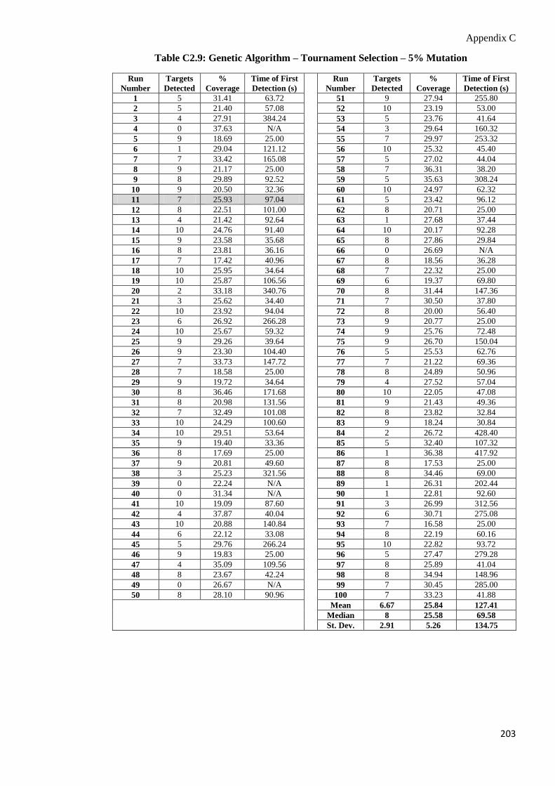
Appendix C
203
Table C2.9: Genetic Algorithm – Tournament Selection – 5% Mutation
Run
Number
Targets
Detected
%
Coverage
Time of First
Detection (s)
Run
Number
Targets
Detected
%
Coverage
Time of First
Detection (s)
1 5 31.41 63.72 51 9 27.94 255.80
2 5 21.40 57.08 52 10 23.19 53.00
3 4 27.91 384.24 53 5 23.76 41.64
4 0 37.63 N/A 54 3 29.64 160.32
5 9 18.69 25.00 55 7 29.97 253.32
6 1 29.04 121.12 56 10 25.32 45.40
7 7 33.42 165.08 57 5 27.02 44.04
8 9 21.17 25.00 58 7 36.31 38.20
9 8 29.89 92.52 59 5 35.63 308.24
10 9 20.50 32.36 60 10 24.97 62.32
11 7 25.93 97.04 61 5 23.42 96.12
12 8 22.51 101.00 62 8 20.71 25.00
13 4 21.42 92.64 63 1 27.68 37.44
14 10 24.76 91.40 64 10 20.17 92.28
15 9 23.58 35.68 65 8 27.86 29.84
16 8 23.81 36.16 66 0 26.69 N/A
17 7 17.42 40.96 67 8 18.56 36.28
18 10 25.95 34.64 68 7 22.32 25.00
19 10 25.87 106.56 69 6 19.37 69.80
20 2 33.18 340.76 70 8 31.44 147.36
21 3 25.62 34.40 71 7 30.50 37.80
22 10 23.92 94.04 72 8 20.00 56.40
23 6 26.92 266.28 73 9 20.77 25.00
24 10 25.67 59.32 74 9 25.76 72.48
25 9 29.26 39.64 75 9 26.70 150.04
26 9 23.30 104.40 76 5 25.53 62.76
27 7 33.73 147.72 77 7 21.22 69.36
28 7 18.58 25.00 78 8 24.89 50.96
29 9 19.72 34.64 79 4 27.52 57.04
30 8 36.46 171.68 80 10 22.05 47.08
31 8 20.98 131.56 81 9 21.43 49.36
32 7 32.49 101.08 82 8 23.82 32.84
33 10 24.29 100.60 83 9 18.24 30.84
34 10 29.51 53.64 84 2 26.72 428.40
35 9 19.40 33.36 85 5 32.40 107.32
36 8 17.69 25.00 86 1 36.38 417.92
37 9 20.81 49.60 87 8 17.53 25.00
38 3 25.23 321.56 88 8 34.46 69.00
39 0 22.24 N/A 89 1 26.31 202.44
40 0 31.34 N/A 90 1 22.81 92.60
41 10 19.09 87.60 91 3 26.99 312.56
42 4 37.87 40.04 92 6 30.71 275.08
43 10 20.88 140.84 93 7 16.58 25.00
44 6 22.12 33.08 94 8 22.19 60.16
45 5 29.76 266.24 95 10 22.82 93.72
46 9 19.83 25.00 96 5 27.47 279.28
47 4 35.09 109.56 97 8 25.89 41.04
48 8 23.67 42.24 98 8 34.94 148.96
49 0 26.67 N/A 99 7 30.45 285.00
50 8 28.10 90.96 100 7 33.23 41.88
Mean 6.67 25.84 127.41
Median 8 25.58 69.58
St. Dev. 2.91 5.26 134.75

Appendix C
204
Table C2.10: Genetic Algorithm – Tournament Selection – 20% Mutation
Run
Number
Targets
Detected
%
Coverage
Time of First
Detection (s)
Run
Number
Targets
Detected
%
Coverage
Time of First
Detection (s)
1 6 34.26 63.68 51 9 33.49 122.56
2 8 33.28 57.08 52 8 26.71 53.08
3 6 32.29 124.64 53 5 27.19 41.64
4 5 36.88 100.88 54 2 31.38 431.72
5 5 33.59 25.00 55 1 30.97 256.64
6 5 34.77 214.72 56 9 29.51 45.44
7 7 27.64 95.12 57 4 28.76 44.08
8 8 27.06 25.00 58 7 31.51 38.24
9 9 33.08 86.00 59 8 38.44 101.08
10 9 26.34 32.36 60 6 34.85 62.28
11 6 36.14 102.16 61 7 31.29 206.60
12 4 31.53 157.00 62 7 29.21 25.00
13 6 33.93 148.04 63 10 36.75 37.44
14 2 36.83 369.76 64 1 30.97 149.40
15 8 34.10 35.68 65 7 29.66 29.84
16 9 25.80 36.16 66 2 31.57 388.68
17 8 33.11 40.96 67 9 27.32 36.32
18 7 34.33 34.60 68 7 28.99 25.00
19 5 34.54 157.60 69 9 29.79 69.80
20 4 39.95 361.96 70 9 28.07 163.04
21 9 31.67 34.04 71 3 30.56 37.84
22 7 31.63 152.80 72 7 33.46 56.40
23 1 35.79 426.52 73 9 25.13 25.00
24 10 32.28 59.32 74 9 34.00 72.48
25 6 32.33 39.64 75 6 36.97 153.76
26 4 34.28 157.96 76 1 34.89 62.80
27 7 32.77 226.92 77 3 31.44 69.40
28 7 32.93 25.00 78 5 35.16 51.00
29 8 31.63 34.64 79 6 29.38 57.04
30 2 33.68 148.80 80 7 37.92 47.08
31 5 33.03 109.12 81 7 35.78 49.36
32 8 37.99 103.96 82 9 30.08 32.84
33 4 33.74 362.48 83 9 31.11 31.08
34 10 32.88 53.64 84 7 35.41 229.56
35 6 26.33 33.36 85 8 37.98 101.64
36 10 23.53 25.00 86 10 32.44 99.00
37 7 31.31 49.60 87 10 24.84 25.00
38 3 37.95 138.92 88 6 34.84 68.96
39 2 37.65 201.56 89 5 27.59 249.64
40 8 33.64 98.64 90 8 32.65 140.88
41 6 28.66 91.08 91 1 35.86 213.72
42 5 31.23 40.04 92 6 39.98 112.92
43 3 36.49 299.64 93 9 33.74 25.00
44 9 29.34 33.08 94 7 25.19 60.16
45 4 34.77 256.08 95 3 33.76 317.16
46 6 34.99 25.00 96 9 30.62 88.20
47 3 29.20 409.64 97 9 31.22 41.04
48 4 31.50 42.24 98 7 38.02 143.28
49 6 29.97 122.24 99 5 35.72 208.44
50 1 36.17 137.96 100 4 36.31 41.88
Mean 6.20 32.47 114.48
Median 7 32.83 69.60
St. Dev. 2.53 3.60 103.17

Appendix C
205
C3 Guided Optimisation Techniques: Individual Results
This section presents the individual results for guided optimisation techniques tested in Section 7.3.
Table C3.1: Guided Random Search
Run
Number
Targets
Detected
%
Coverage
Time of First
Detection (s)
Run
Number
Targets
Detected
%
Coverage
Time of First
Detection (s)
1 8 35.06 60.20 51 9 34.10 209.32
2 8 29.70 57.04 52 10 29.18 48.16
3 9 34.97 123.72 53 8 29.87 41.64
4 9 30.84 71.16 54 9 31.68 86.52
5 9 27.52 25.00 55 8 28.26 73.36
6 0 40.19 N/A 56 9 26.89 45.44
7 9 34.66 177.88 57 10 25.82 44.08
8 10 30.48 25.00 58 6 37.42 38.24
9 10 28.99 73.40 59 5 37.41 126.84
10 9 21.55 32.36 60 8 25.66 62.04
11 9 32.60 171.76 61 8 40.13 195.36
12 10 31.80 194.40 62 10 27.89 25.00
13 10 33.77 183.48 63 9 26.49 37.44
14 0 35.09 N/A 64 10 33.84 145.68
15 10 28.73 35.68 65 9 27.81 29.84
16 10 27.56 36.16 66 2 34.67 146.80
17 9 26.12 40.96 67 9 26.62 36.32
18 10 30.49 34.64 68 10 22.40 25.00
19 8 33.03 85.72 69 10 31.75 68.96
20 9 27.57 109.48 70 8 29.68 31.04
21 10 30.96 34.04 71 10 32.23 37.84
22 9 27.00 64.56 72 10 28.01 56.48
23 8 33.54 196.24 73 10 26.56 25.00
24 10 29.92 59.32 74 10 34.78 72.88
25 10 34.19 39.60 75 10 30.74 130.40
26 9 36.32 172.24 76 8 27.61 62.56
27 10 28.33 87.68 77 10 28.98 69.20
28 10 27.09 25.00 78 10 31.66 51.00
29 9 27.71 34.64 79 9 30.13 57.04
30 9 34.68 81.68 80 5 33.65 47.08
31 6 30.35 184.20 81 9 34.92 49.36
32 10 29.37 81.84 82 9 30.65 32.84
33 10 30.64 65.52 83 10 25.62 30.80
34 10 30.28 53.64 84 8 35.12 116.00
35 9 33.41 33.36 85 10 31.25 114.36
36 10 27.42 25.00 86 7 41.33 278.32
37 7 30.74 49.60 87 10 27.57 25.00
38 9 31.94 92.36 88 9 35.53 68.88
39 10 31.69 72.44 89 8 27.58 61.56
40 7 29.14 59.52 90 10 33.47 158.56
41 7 31.73 123.20 91 9 33.98 84.16
42 9 30.53 40.04 92 10 31.01 87.00
43 9 30.84 50.40 93 8 26.00 25.00
44 9 28.34 33.08 94 9 27.81 60.20
45 8 31.84 65.88 95 10 30.48 114.60
46 9 31.01 25.00 96 9 32.21 157.44
47 8 38.88 237.92 97 8 32.91 41.04
48 9 32.54 42.24 98 8 35.57 324.48
49 10 30.21 78.00 99 10 29.08 113.84
50 10 26.14 101.28 100 8 34.21 41.88
Mean 8.74 30.96 90.39
Median 9 30.69 61.80
St. Dev. 1.82 3.68 87.96

Appendix C
206
Table C3.2: Guided Distinct Regions Random Search
Run
Number
Targets
Detected
%
Coverage
Time of First
Detection (s)
Run
Number
Targets
Detected
%
Coverage
Time of First
Detection (s)
1 4 35.59 60.28 51 3 36.71 354.08
2 4 31.69 57.04 52 7 28.97 54.08
3 7 35.88 89.20 53 6 29.96 41.64
4 7 34.07 101.80 54 8 33.60 243.24
5 6 31.30 25.00 55 4 37.46 93.72
6 6 36.94 252.52 56 8 31.81 45.40
7 5 35.54 72.96 57 9 27.83 44.08
8 8 27.19 25.00 58 8 33.19 38.20
9 4 37.41 181.72 59 7 36.41 126.16
10 10 29.45 32.36 60 9 32.83 62.04
11 9 35.44 112.68 61 8 34.71 112.16
12 3 34.49 131.96 62 6 31.03 25.00
13 6 31.87 113.76 63 9 33.47 37.44
14 8 34.66 127.64 64 7 34.48 255.88
15 8 31.50 35.68 65 9 29.70 29.84
16 9 32.00 36.16 66 10 34.75 112.64
17 9 26.53 40.96 67 9 32.12 36.32
18 6 33.05 34.64 68 7 29.57 25.00
19 7 32.38 99.24 69 7 37.26 69.00
20 8 31.67 142.60 70 10 34.36 88.84
21 7 34.51 34.08 71 8 30.67 37.84
22 6 33.29 73.00 72 8 31.73 56.36
23 7 35.89 273.56 73 9 30.16 25.00
24 10 30.02 59.32 74 5 38.18 72.44
25 8 31.38 39.60 75 7 33.99 123.40
26 6 34.36 100.28 76 7 31.89 62.56
27 8 33.45 116.24 77 9 31.80 69.16
28 9 28.99 25.00 78 5 33.02 51.00
29 9 31.44 34.64 79 7 32.59 57.04
30 4 35.67 282.24 80 6 34.48 47.08
31 5 37.46 127.44 81 8 33.26 49.36
32 7 29.82 143.04 82 8 28.30 32.84
33 7 34.75 60.16 83 8 28.83 31.08
34 7 33.41 53.64 84 9 31.98 177.36
35 9 34.48 33.36 85 9 33.86 98.88
36 8 22.10 25.00 86 6 36.91 269.08
37 9 26.69 49.60 87 8 25.90 25.00
38 9 30.88 160.16 88 7 32.08 68.84
39 9 31.61 85.28 89 8 27.04 62.00
40 7 31.94 99.40 90 8 33.34 114.04
41 6 34.42 255.80 91 8 33.22 105.36
42 8 35.63 40.04 92 8 34.42 190.92
43 9 32.66 146.16 93 6 33.40 25.00
44 4 31.91 33.08 94 8 33.61 60.16
45 5 33.92 81.28 95 7 34.96 122.44
46 9 23.06 25.00 96 5 33.21 77.32
47 7 34.64 126.20 97 8 38.35 41.01
48 5 27.71 42.24 98 5 38.50 115.32
49 9 31.14 98.28 99 9 31.87 182.00
50 9 31.86 118.40 100 4 34.50 41.88
Mean 7.25 32.64 90.01
Median 8 33.12 65.70
St. Dev. 1.70 3.13 68.98

Appendix C
207
Table C3.3: Guided Hill Climbing
Run
Number
Targets
Detected
%
Coverage
Time of First
Detection (s)
Run
Number
Targets
Detected
%
Coverage
Time of First
Detection (s)
1 9 26.80 63.68 51 7 29.18 237.16
2 7 24.10 57.08 52 10 23.68 47.84
3 3 20.16 358.96 53 8 23.73 41.64
4 8 27.79 251.56 54 6 32.52 237.96
5 9 20.73 25.00 55 9 25.33 77.32
6 4 32.40 195.24 56 10 28.06 45.44
7 7 24.48 84.68 57 10 23.86 44.08
8 8 23.85 25.00 58 8 30.89 38.20
9 8 26.01 109.68 59 0 27.92 N/A
10 10 22.31 32.36 60 9 27.73 62.20
11 9 23.72 66.68 61 8 25.53 153.48
12 4 26.07 280.04 62 10 21.83 25.00
13 8 25.19 170.76 63 8 26.64 37.44
14 9 22.97 147.12 64 6 21.90 228.32
15 7 24.18 35.68 65 10 23.41 29.84
16 10 25.29 36.16 66 1 28.24 375.68
17 8 23.60 40.96 67 6 24.20 36.32
18 7 27.91 34.64 68 9 18.39 25.00
19 9 24.28 144.96 69 7 25.56 69.76
20 3 28.70 376.80 70 10 24.55 72.24
21 9 25.58 34.04 71 10 27.46 37.84
22 8 25.72 127.48 72 9 25.00 56.36
23 10 23.93 139.16 73 10 20.96 25.00
24 7 27.35 59.28 74 9 30.38 72.40
25 8 28.57 39.64 75 10 26.89 118.04
26 9 26.10 152.44 76 9 25.51 62.60
27 9 22.98 176.00 77 6 24.74 69.24
28 9 22.91 25.00 78 8 27.03 51.00
29 9 23.81 34.64 79 7 27.43 57.04
30 7 28.83 117.08 80 10 27.86 47.08
31 3 25.64 320.00 81 7 27.17 49.36
32 6 27.23 304.68 82 8 25.30 32.84
33 8 21.77 68.64 83 9 25.83 31.08
34 9 30.05 53.64 84 7 28.88 116.28
35 8 21.81 33.36 85 8 28.48 169.64
36 9 19.76 25.00 86 8 27.48 256.44
37 9 24.60 49.64 87 10 21.09 25.00
38 9 24.57 169.36 88 7 33.64 68.88
39 7 27.61 248.32 89 10 20.91 81.16
40 9 27.35 172.08 90 10 22.89 92.60
41 10 24.37 185.80 91 4 26.00 335.20
42 10 27.07 40.04 92 9 25.50 164.48
43 6 27.40 134.56 93 7 23.28 25.00
44 9 24.39 33.08 94 8 30.23 60.16
45 6 25.74 138.68 95 8 25.30 205.04
46 10 29.48 25.00 96 2 24.93 172.76
47 4 24.35 239.40 97 7 28.05 41.04
48 8 27.70 42.24 98 7 29.30 128.32
49 0 24.86 N/A 99 9 28.04 144.04
50 8 28.97 94.92 100 8 30.47 41.88
Mean 7.73 25.80 116.23
Median 8 25.57 68.76
St. Dev. 2.22 2.88 108.70

Appendix C
208
Table C3.4: Guided Random Restart Hill Climbing
Run
Number
Targets
Detected
%
Coverage
Time of First
Detection (s)
Run
Number
Targets
Detected
%
Coverage
Time of First
Detection (s)
1 6 27.37 60.44 51 9 24.88 167.08
2 6 27.80 57.08 52 8 21.28 49.52
3 0 28.29 N/A 53 8 23.47 41.64
4 8 28.87 160.72 54 8 27.60 190.88
5 9 23.63 25.00 55 8 25.85 221.04
6 0 27.93 N/A 56 8 27.94 45.40
7 4 27.34 228.88 57 10 26.01 44.04
8 7 22.86 25.00 58 5 29.16 38.20
9 6 29.45 235.36 59 0 31.17 N/A
10 10 22.58 32.36 60 9 29.82 62.08
11 6 30.11 67.64 61 7 26.46 129.04
12 4 29.44 177.52 62 10 25.65 25.00
13 7 27.49 186.12 63 2 22.73 37.44
14 10 22.36 101.76 64 9 25.58 146.48
15 10 24.84 35.68 65 10 22.23 29.84
16 9 22.43 36.16 66 0 25.87 N/A
17 10 20.99 40.96 67 9 23.81 36.32
18 10 25.41 34.60 68 9 20.69 25.00
19 7 27.23 248.24 69 10 26.90 69.04
20 6 31.93 309.16 70 9 22.19 62.24
21 8 25.13 34.40 71 9 30.93 37.84
22 10 24.88 63.92 72 6 23.22 56.36
23 4 26.35 150.32 73 10 23.60 25.00
24 10 26.06 59.32 74 9 30.10 72.44
25 8 27.88 39.60 75 3 27.68 321.72
26 3 28.65 308.12 76 7 28.94 62.60
27 1 26.78 364.04 77 9 27.40 105.96
28 10 28.86 25.00 78 8 24.51 51.00
29 6 25.52 34.64 79 4 29.28 57.04
30 7 27.28 272.80 80 4 30.32 47.08
31 1 29.46 212.08 81 7 27.81 49.36
32 8 30.11 236.08 82 10 21.43 32.84
33 10 26.50 111.04 83 8 22.75 31.08
34 9 25.26 53.64 84 9 31.40 188.80
35 8 28.40 33.36 85 3 25.78 252.36
36 9 18.05 25.00 86 5 26.58 78.24
37 8 23.76 49.60 87 10 20.63 25.00
38 7 29.56 167.48 88 9 25.94 68.88
39 4 33.94 292.88 89 8 21.01 57.32
40 3 31.10 244.12 90 7 28.16 106.16
41 10 23.43 74.24 91 8 26.02 93.56
42 8 28.83 40.04 92 9 25.50 115.84
43 10 24.09 141.68 93 8 24.99 25.00
44 9 26.91 33.08 94 9 25.51 60.16
45 7 29.67 211.68 95 8 26.89 115.80
46 9 24.97 25.00 96 2 26.36 239.80
47 6 31.32 182.48 97 9 27.91 41.04
48 7 29.11 42.24 98 7 30.74 138.16
49 9 24.47 80.28 99 10 26.74 131.08
50 5 26.55 187.64 100 7 26.71 41.88
Mean 7.19 26.45 121.68
Median 8 26.56 63.26
St. Dev. 2.71 2.98 120.41

Appendix C
209
Table C3.5: Guided Simulated Annealing
Run
Number
Targets
Detected
%
Coverage
Time of First
Detection (s)
Run
Number
Targets
Detected
%
Coverage
Time of First
Detection (s)
1 6 31.51 60.28 51 10 27.53 202.88
2 8 23.53 57.04 52 8 27.76 48.12
3 6 27.47 104.80 53 3 22.69 41.64
4 8 29.46 172.80 54 2 27.74 392.40
5 7 25.19 25.00 55 5 31.13 251.28
6 0 27.26 N/A 56 10 25.89 45.44
7 10 26.14 122.04 57 6 30.13 44.04
8 9 25.97 25.00 58 9 30.58 38.20
9 8 26.03 67.08 59 0 28.30 N/A
10 8 22.41 32.36 60 9 27.78 62.24
11 10 25.31 86.04 61 8 25.87 131.80
12 10 27.24 80.24 62 10 27.83 25.00
13 8 26.08 98.20 63 7 26.69 37.44
14 6 26.72 189.60 64 7 27.25 101.12
15 10 23.77 35.68 65 10 21.80 29.84
16 10 26.00 36.16 66 8 32.38 272.56
17 10 27.71 40.96 67 9 23.30 36.28
18 10 27.04 34.64 68 8 25.25 25.00
19 8 26.21 97.52 69 9 24.89 68.32
20 9 26.98 104.32 70 10 25.06 111.36
21 10 26.71 34.04 71 8 27.73 37.84
22 9 26.50 101.44 72 8 24.29 56.40
23 0 25.31 N/A 73 10 26.60 25.00
24 10 26.89 59.32 74 8 28.51 72.40
25 9 25.34 39.60 75 8 29.19 98.76
26 8 30.86 148.36 76 7 26.19 62.76
27 10 20.69 90.84 77 9 24.05 69.08
28 9 29.83 25.00 78 8 33.12 51.00
29 9 26.12 34.64 79 8 27.55 57.04
30 8 27.70 106.48 80 9 24.72 47.08
31 5 26.69 117.64 81 8 28.22 49.36
32 8 31.53 261.84 82 9 26.73 32.84
33 9 26.83 59.88 83 8 32.96 31.08
34 9 29.87 53.64 84 8 26.94 168.76
35 6 30.10 33.36 85 1 27.17 376.72
36 10 21.47 25.00 86 10 28.96 139.08
37 10 28.06 49.60 87 10 20.11 25.00
38 4 31.01 287.60 88 7 26.50 68.92
39 8 26.10 128.08 89 8 22.58 113.64
40 0 27.87 N/A 90 1 25.80 426.64
41 10 24.00 150.24 91 3 27.29 103.00
42 6 28.20 40.04 92 7 24.26 77.92
43 8 25.20 122.68 93 9 26.98 25.00
44 8 27.44 33.08 94 9 27.76 60.12
45 7 24.94 100.92 95 7 27.12 187.72
46 9 27.49 25.00 96 6 34.66 115.44
47 4 27.52 156.68 97 8 24.39 41.04
48 5 26.78 42.24 98 0 27.77 N/A
49 0 27.28 N/A 99 8 24.83 104.80
50 0 25.63 N/A 100 9 26.90 41.88
Mean 7.36 26.88 123.08
Median 8 26.89 67.70
St. Dev. 2.82 2.58 139.32

Appendix C
210
Table C3.6: Guided Random Restart Simulated Annealing
Run
Number
Targets
Detected
%
Coverage
Time of First
Detection (s)
Run
Number
Targets
Detected
%
Coverage
Time of First
Detection (s)
1 5 31.79 60.28 51 10 31.98 60.96
2 7 26.43 57.00 52 7 31.08 53.88
3 5 27.24 231.40 53 8 26.86 41.64
4 8 26.24 72.88 54 9 26.37 106.16
5 10 26.92 25.00 55 0 28.37 N/A
6 0 30.60 N/A 56 10 33.90 45.44
7 6 29.05 101.44 57 9 24.42 44.04
8 10 25.31 25.00 58 8 32.56 38.24
9 6 25.81 168.44 59 9 25.34 101.00
10 9 30.15 32.36 60 8 30.50 62.04
11 10 24.95 221.92 61 8 28.32 93.16
12 5 30.95 200.04 62 9 30.22 25.00
13 8 28.39 89.36 63 8 30.44 37.44
14 9 28.16 202.16 64 10 21.16 111.08
15 10 30.77 35.68 65 8 29.06 29.84
16 6 27.56 36.16 66 0 25.04 N/A
17 9 32.78 40.96 67 7 28.01 36.28
18 10 33.32 34.64 68 7 23.90 25.00
19 9 25.63 109.56 69 10 29.23 68.44
20 0 30.00 N/A 70 9 28.33 245.44
21 10 27.08 34.40 71 9 30.80 37.80
22 6 26.34 173.24 72 7 24.15 56.44
23 9 25.87 181.32 73 10 27.63 25.00
24 9 26.42 59.32 74 10 30.84 72.52
25 8 28.61 39.60 75 0 26.27 N/A
26 8 28.12 113.68 76 10 21.31 62.56
27 10 29.09 139.64 77 9 28.72 61.80
28 9 21.51 25.00 78 8 28.64 51.00
29 9 28.91 34.64 79 2 27.93 57.04
30 9 26.75 195.72 80 10 25.88 47.04
31 7 27.37 63.08 81 10 28.26 49.36
32 8 25.91 197.04 82 10 31.39 32.84
33 10 25.97 71.76 83 8 31.77 31.08
34 10 28.16 53.64 84 7 29.38 262.24
35 8 29.01 33.36 85 7 27.20 103.08
36 8 28.02 25.00 86 9 25.49 93.64
37 6 26.55 49.60 87 10 24.79 25.00
38 7 28.47 126.64 88 8 32.09 68.92
39 3 26.57 328.92 89 8 21.32 57.96
40 6 30.72 75.52 90 9 27.84 246.12
41 8 27.64 77.72 91 10 24.50 111.36
42 9 27.50 40.04 92 8 28.63 76.04
43 10 27.63 103.08 93 10 27.66 25.00
44 8 30.11 33.08 94 9 24.74 60.28
45 8 27.39 72.40 95 8 27.16 222.32
46 10 31.42 25.00 96 9 26.95 118.80
47 4 28.07 179.64 97 10 26.58 41.04
48 7 31.00 42.24 98 6 26.49 237.12
49 9 30.89 161.72 99 1 28.72 386.16
50 7 29.91 165.60 100 8 31.67 41.88
Mean 7.76 27.99 113.52
Median 8 28.02 62.30
St. Dev. 2.52 2.62 122.43

Appendix C
211
Table C3.7: Guided Ant Colony Optimisation
Run
Number
Targets
Detected
%
Coverage
Time of First
Detection (s)
Run
Number
Targets
Detected
%
Coverage
Time of First
Detection (s)
1 7 24.25 63.68 51 10 24.90 172.80
2 8 24.85 57.08 52 6 21.25 52.92
3 0 24.39 N/A 53 5 17.79 41.64
4 9 23.71 116.00 54 1 26.34 437.60
5 9 23.12 25.00 55 9 21.71 135.00
6 2 25.24 248.52 56 7 25.74 45.40
7 0 23.03 N/A 57 8 22.62 44.04
8 9 24.94 25.00 58 7 25.54 38.20
9 8 27.97 182.76 59 7 24.26 175.76
10 9 25.21 32.36 60 8 25.53 62.28
11 8 26.60 335.48 61 2 27.61 227.32
12 6 24.09 287.32 62 10 23.34 25.00
13 1 26.24 231.48 63 1 29.02 37.44
14 10 20.23 117.68 64 8 23.88 142.52
15 10 24.33 35.68 65 10 21.47 29.84
16 9 18.96 36.16 66 1 23.13 329.76
17 8 20.05 40.96 67 8 16.79 36.32
18 6 23.12 34.64 68 9 21.44 25.00
19 4 25.61 116.84 69 2 27.51 69.80
20 8 27.85 194.80 70 10 21.81 31.20
21 9 23.89 34.40 71 9 26.19 37.84
22 1 27.32 404.16 72 7 19.66 56.40
23 8 20.77 99.32 73 10 23.56 25.00
24 9 22.34 59.28 74 2 25.85 72.48
25 9 25.17 39.60 75 8 24.66 118.52
26 7 21.82 114.12 76 6 24.33 62.76
27 7 26.49 215.40 77 1 24.64 69.40
28 9 20.86 25.00 78 9 21.90 51.00
29 10 16.54 34.64 79 9 24.29 57.08
30 4 27.66 226.28 80 3 24.35 47.04
31 0 25.16 N/A 81 8 25.13 49.36
32 8 21.42 122.00 82 9 21.66 32.84
33 9 23.59 157.00 83 8 20.30 30.84
34 10 26.24 53.64 84 0 27.36 N/A
35 8 19.45 33.36 85 0 25.24 N/A
36 9 20.23 25.00 86 9 23.12 214.20
37 8 22.12 49.60 87 10 17.27 25.00
38 1 24.80 444.08 88 8 20.24 68.96
39 0 26.46 N/A 89 3 20.76 244.56
40 1 24.63 101.80 90 10 24.90 193.28
41 8 22.20 90.56 91 3 27.65 297.08
42 6 26.01 40.04 92 4 26.16 335.28
43 10 19.65 84.92 93 7 21.16 25.00
44 6 23.45 33.08 94 7 22.10 60.16
45 1 23.28 101.84 95 5 25.97 158.84
46 10 20.77 25.00 96 1 28.94 436.00
47 0 24.84 N/A 97 9 25.31 41.04
48 5 23.90 42.24 98 1 26.79 166.40
49 9 24.79 141.76 99 0 25.88 N/A
50 0 27.19 N/A 100 5 26.51 41.88
Mean 6.13 23.80 150.18
Median 8 24.31 69.18
St. Dev. 3.44 2.72 159.72

Appendix C
212
Table C3.8: Guided Particle Swarm Optimisation
Run
Number
Targets
Detected
%
Coverage
Time of First
Detection (s)
Run
Number
Targets
Detected
%
Coverage
Time of First
Detection (s)
1 9 24.37 63.72 51 8 24.10 121.44
2 10 24.40 57.08 52 8 27.87 52.84
3 0 18.61 N/A 53 7 19.70 41.64
4 9 29.95 124.36 54 7 29.66 287.56
5 7 23.36 25.00 55 9 25.63 101.00
6 8 29.48 177.88 56 10 28.15 45.44
7 8 23.65 108.96 57 9 25.71 44.08
8 7 26.15 25.00 58 9 25.43 38.20
9 8 19.31 91.80 59 7 32.80 136.28
10 9 19.75 32.36 60 8 30.74 62.32
11 10 19.50 96.80 61 1 28.03 329.88
12 8 31.03 158.36 62 9 33.38 25.00
13 8 21.39 97.68 63 10 27.01 37.44
14 9 24.55 115.76 64 8 26.12 99.56
15 10 27.81 35.68 65 8 30.77 29.84
16 9 26.66 36.16 66 10 23.08 113.88
17 10 28.14 40.96 67 10 21.77 36.32
18 7 27.50 34.64 68 9 23.34 25.00
19 9 31.53 138.36 69 8 21.81 69.80
20 8 29.63 105.28 70 10 21.25 86.00
21 8 28.93 34.04 71 10 24.71 37.84
22 9 23.16 114.88 72 8 24.42 56.40
23 8 30.65 266.56 73 9 32.24 25.00
24 9 25.99 59.28 74 8 32.53 72.48
25 8 22.39 39.64 75 10 30.74 108.36
26 8 21.61 117.44 76 8 28.02 62.76
27 6 27.11 241.32 77 7 28.23 69.40
28 10 26.40 25.00 78 10 25.71 50.96
29 10 26.22 34.64 79 9 22.71 57.04
30 8 31.73 181.32 80 9 22.39 47.04
31 4 27.83 165.84 81 6 27.97 49.36
32 10 21.98 97.24 82 9 25.22 32.84
33 5 21.05 90.84 83 8 21.56 31.08
34 9 27.52 53.64 84 8 33.05 196.08
35 7 23.18 33.36 85 8 26.70 109.04
36 8 19.14 25.00 86 6 34.62 132.92
37 10 17.60 49.60 87 10 23.98 25.00
38 8 25.07 155.32 88 8 23.77 69.00
39 6 33.89 111.68 89 9 19.46 158.92
40 2 27.26 369.68 90 9 24.71 92.28
41 9 23.70 99.64 91 3 31.67 229.64
42 8 28.40 40.04 92 9 28.40 92.72
43 8 27.00 133.72 93 9 27.75 25.00
44 9 29.48 33.08 94 8 23.14 60.16
45 6 23.43 131.68 95 10 22.98 93.56
46 9 30.34 25.00 96 9 25.47 154.72
47 7 30.85 123.56 97 10 26.48 41.04
48 8 23.07 42.24 98 6 31.52 138.92
49 10 25.98 138.56 99 9 26.42 180.24
50 9 26.16 193.72 100 10 29.26 41.88
Mean 8.16 26.16 96.59
Median 8 26.15 69.60
St. Dev. 1.86 3.87 82.08

Appendix C
213
Table C3.9: Guided Genetic Algorithm – Elitist – 20% Mutation
Run
Number
Targets
Detected
%
Coverage
Time of First
Detection (s)
Run
Number
Targets
Detected
%
Coverage
Time of First
Detection (s)
1 7 33.43 63.72 51 9 32.60 275.16
2 3 32.99 57.08 52 8 31.22 53.04
3 3 30.95 149.72 53 6 20.13 41.64
4 7 36.81 118.56 54 9 33.35 154.68
5 5 30.97 25.00 55 7 34.68 90.76
6 7 35.85 145.56 56 6 34.74 45.40
7 5 26.17 235.36 57 9 29.88 44.04
8 7 26.16 25.00 58 7 34.73 38.16
9 4 29.43 86.00 59 7 31.40 102.72
10 10 27.06 32.36 60 7 35.90 62.28
11 8 31.40 136.88 61 3 33.19 251.72
12 10 29.34 118.80 62 9 32.35 25.00
13 5 31.43 118.96 63 4 36.51 37.44
14 8 33.27 136.92 64 4 27.83 93.08
15 10 28.50 35.68 65 7 27.63 29.84
16 9 29.48 36.16 66 4 34.41 264.60
17 6 26.47 40.96 67 8 28.41 36.32
18 4 25.54 34.60 68 8 33.72 25.00
19 8 35.80 114.92 69 10 30.73 69.80
20 3 31.02 154.52 70 8 27.24 182.36
21 8 34.02 34.40 71 7 32.66 37.84
22 7 39.62 104.12 72 7 28.39 56.40
23 9 33.24 156.84 73 8 28.66 25.00
24 10 30.08 59.28 74 7 35.52 72.48
25 5 31.26 39.60 75 8 32.96 105.64
26 8 32.59 141.40 76 6 32.72 62.76
27 2 31.23 134.92 77 8 29.46 69.36
28 7 29.54 25.00 78 2 34.56 51.00
29 6 28.14 34.64 79 6 34.76 57.04
30 4 36.01 107.76 80 8 35.19 47.08
31 5 26.00 136.96 81 9 30.31 49.36
32 9 30.40 101.40 82 8 30.70 32.84
33 2 26.24 176.52 83 10 25.93 31.08
34 8 32.20 53.64 84 8 37.01 114.48
35 5 25.13 33.36 85 7 33.34 102.76
36 10 31.14 25.00 86 2 36.83 97.04
37 8 30.02 49.60 87 10 22.98 25.00
38 5 37.36 194.16 88 9 31.39 68.96
39 7 31.19 110.32 89 9 30.78 92.68
40 1 32.49 416.20 90 2 30.94 250.24
41 3 33.30 263.68 91 3 28.66 158.80
42 8 31.31 40.04 92 5 29.78 95.80
43 0 25.33 N/A 93 6 27.58 25.00
44 8 26.88 33.04 94 10 34.78 60.16
45 6 30.64 216.44 95 5 37.37 103.00
46 7 40.42 25.00 96 10 32.80 133.68
47 5 32.85 222.12 97 4 35.47 41.04
48 4 29.14 42.24 98 2 35.43 311.72
49 7 34.77 135.36 99 7 26.96 86.28
50 6 26.80 168.24 100 5 36.93 41.88
Mean 6.47 31.43 101.17
Median 7 31.28 69.58
St. Dev. 2.41 3.70 87.19

Appendix C
214
Table C3.10: Guided Genetic Algorithm – Roulette Wheel – 20% Mutation
Run
Number
Targets
Detected
%
Coverage
Time of First
Detection (s)
Run
Number
Targets
Detected
%
Coverage
Time of First
Detection (s)
1 8 35.52 63.72 51 10 34.61 166.84
2 9 26.32 57.08 52 10 19.98 53.00
3 6 34.75 154.64 53 8 25.60 41.64
4 3 36.64 309.28 54 1 34.25 322.76
5 9 29.03 25.00 55 4 29.30 159.20
6 5 28.92 121.12 56 10 27.90 45.44
7 9 30.61 111.00 57 8 22.86 44.08
8 7 25.64 25.00 58 6 31.10 38.20
9 7 34.66 109.08 59 1 35.21 303.12
10 8 26.90 32.36 60 6 36.65 62.32
11 9 30.71 106.16 61 8 34.45 198.56
12 9 27.64 114.80 62 10 25.32 25.00
13 4 29.43 92.76 63 7 36.18 37.44
14 10 30.42 133.00 64 3 26.14 92.80
15 9 32.49 35.68 65 7 25.53 29.84
16 10 30.72 36.16 66 5 32.42 152.68
17 10 27.18 40.96 67 5 22.03 36.28
18 9 34.28 34.64 68 6 25.14 25.00
19 2 28.51 166.84 69 9 28.41 69.80
20 8 32.60 246.60 70 9 25.44 92.16
21 9 29.32 34.40 71 9 31.77 37.84
22 9 26.27 94.00 72 8 25.40 56.40
23 8 32.92 261.36 73 9 28.50 25.00
24 10 31.62 59.32 74 9 32.89 72.48
25 8 31.22 39.60 75 5 32.61 354.60
26 3 28.59 139.12 76 7 29.67 62.76
27 6 30.06 102.00 77 7 28.48 69.36
28 7 36.56 25.00 78 7 27.55 51.00
29 9 25.57 34.64 79 8 29.33 57.04
30 5 32.99 117.08 80 9 27.59 47.04
31 2 32.88 96.04 81 10 23.43 49.36
32 8 30.47 138.96 82 9 26.54 32.84
33 2 31.62 419.16 83 8 30.07 30.84
34 8 32.29 53.64 84 7 35.27 168.80
35 7 34.54 33.36 85 9 28.94 101.64
36 8 23.36 25.00 86 6 31.79 288.36
37 9 26.12 49.60 87 10 26.11 25.00
38 2 32.12 209.08 88 7 33.34 68.96
39 8 29.99 149.48 89 9 26.71 96.64
40 4 28.06 387.76 90 5 31.07 201.04
41 6 25.53 94.96 91 7 37.36 154.84
42 9 31.18 40.04 92 6 30.59 146.96
43 7 28.44 152.12 93 7 26.04 25.00
44 5 36.20 33.08 94 9 27.48 60.16
45 7 34.31 146.56 95 6 35.69 164.24
46 8 29.92 25.00 96 9 31.65 88.12
47 5 36.93 141.12 97 8 35.10 41.04
48 7 31.58 42.24 98 1 37.27 418.08
49 8 35.99 216.08 99 8 27.00 165.20
50 8 30.47 137.04 100 8 30.71 41.88
Mean 7.13 30.25 107.11
Median 8 30.44 69.58
St. Dev. 2.30 3.86 92.31

Appendix C
215
Table C3.11: Guided Genetic Algorithm – Tournament Selection – 20% Mutation
Run
Number
Targets
Detected
%
Coverage
Time of First
Detection (s)
Run
Number
Targets
Detected
%
Coverage
Time of First
Detection (s)
1 5 30.43 63.72 51 9 33.33 119.40
2 8 26.74 57.08 52 7 31.14 53.00
3 4 34.07 169.28 53 7 26.57 41.64
4 9 28.98 139.56 54 7 31.79 111.12
5 5 35.19 25.00 55 8 30.17 99.96
6 5 31.18 181.84 56 10 29.56 45.44
7 10 32.03 255.20 57 8 29.26 44.04
8 9 29.06 25.00 58 8 33.10 38.20
9 6 28.60 86.00 59 1 34.50 293.28
10 8 32.39 32.36 60 7 34.20 62.28
11 5 30.92 192.56 61 2 29.80 94.92
12 5 33.21 106.28 62 9 30.20 25.00
13 7 29.30 93.80 63 4 32.92 37.44
14 6 25.16 108.96 64 8 30.74 114.48
15 7 33.60 35.68 65 9 29.52 29.84
16 9 30.87 36.16 66 1 29.79 326.52
17 9 28.64 40.96 67 8 27.78 36.32
18 6 31.29 34.64 68 8 23.62 25.00
19 7 35.13 166.96 69 8 30.21 69.80
20 2 36.29 105.44 70 2 23.39 185.92
21 9 32.41 34.40 71 7 28.53 37.84
22 9 27.05 94.00 72 9 29.97 56.40
23 0 29.80 N/A 73 7 28.38 25.00
24 10 28.85 59.32 74 4 32.73 72.48
25 6 32.92 39.64 75 8 32.89 139.08
26 8 31.92 101.72 76 4 27.04 62.80
27 8 28.91 102.84 77 5 29.75 69.40
28 9 25.01 25.00 78 6 33.69 51.00
29 8 30.07 34.64 79 6 34.60 57.04
30 8 31.00 105.96 80 5 33.19 47.08
31 7 33.21 110.52 81 4 31.10 49.36
32 7 33.98 103.16 82 8 32.42 32.84
33 5 27.11 102.16 83 8 26.32 31.08
34 9 32.71 53.64 84 7 33.80 162.32
35 6 32.83 33.36 85 8 34.25 98.40
36 8 22.61 25.00 86 9 32.78 115.52
37 10 25.90 49.60 87 9 19.32 25.00
38 2 30.29 175.92 88 7 26.95 69.00
39 7 30.16 136.48 89 7 25.07 189.64
40 0 27.76 N/A 90 1 30.74 321.80
41 5 28.01 88.24 91 6 30.21 187.24
42 2 26.77 40.04 92 8 31.31 225.32
43 8 29.09 145.92 93 7 27.42 25.00
44 3 27.38 33.08 94 7 30.61 60.16
45 5 30.30 138.12 95 0 28.55 N/A
46 7 33.99 25.00 96 4 31.50 88.20
47 2 33.90 187.60 97 7 31.37 41.04
48 6 37.04 42.24 98 7 31.03 131.04
49 3 28.67 172.24 99 10 26.85 136.20
50 4 29.26 141.68 100 8 33.93 41.88
Mean 6.37 30.30 104.81
Median 7 30.29 69.60
St. Dev. 2.53 3.12 101.62

Appendix C
216
C4 Hybrid Algorithms: Individual Results
This section presents the individual results for the hybrid algorithms tested in Section 8.2.
Table C4.1: Random Search with Guided Hill Climbing
Run
Number
Targets
Detected
%
Coverage
Time of First
Detection (s)
Run
Number
Targets
Detected
%
Coverage
Time of First
Detection (s)
1 8 21.91 60.28 51 10 30.97 160.48
2 8 20.97 57.04 52 10 20.83 54.00
3 8 34.15 204.16 53 6 16.75 41.64
4 4 43.52 295.32 54 9 24.11 118.84
5 9 16.53 25.00 55 8 29.03 124.20
6 9 26.46 134.96 56 10 16.97 45.44
7 10 17.34 54.60 57 10 17.66 44.08
8 10 18.23 25.00 58 10 19.52 38.20
9 10 24.09 87.12 59 6 30.85 182.24
10 9 16.08 32.36 60 9 19.80 62.04
11 9 34.55 198.08 61 10 30.85 148.92
12 9 19.73 105.04 62 10 16.55 25.00
13 9 24.65 126.36 63 9 15.79 37.44
14 5 44.31 368.92 64 10 31.07 180.24
15 10 15.32 35.68 65 9 18.83 29.84
16 9 17.55 36.16 66 9 20.22 52.92
17 10 15.71 40.96 67 9 18.80 36.32
18 8 19.79 34.64 68 10 20.44 25.00
19 9 22.45 89.36 69 10 20.72 68.96
20 10 21.53 72.68 70 9 23.38 133.88
21 8 17.40 34.04 71 10 17.71 37.84
22 9 37.22 256.52 72 8 18.16 56.52
23 10 22.89 66.00 73 10 16.23 25.00
24 10 20.78 59.32 74 8 24.13 72.36
25 7 16.02 39.64 75 5 42.76 319.28
26 8 20.15 51.80 76 10 20.49 62.56
27 10 16.61 84.84 77 10 19.03 69.16
28 10 15.20 25.00 78 10 16.30 51.00
29 8 17.51 34.64 79 9 18.98 57.04
30 9 25.90 84.04 80 9 14.40 47.04
31 8 21.21 68.08 81 9 16.48 49.36
32 9 24.06 84.80 82 10 17.07 32.84
33 10 20.55 65.24 83 7 17.03 30.80
34 7 23.00 53.64 84 9 22.89 92.76
35 7 16.47 33.36 85 10 25.11 105.00
36 9 18.22 25.00 86 10 24.50 83.68
37 10 17.35 49.60 87 10 16.74 25.00
38 9 32.14 180.92 88 8 19.27 68.88
39 7 21.86 69.60 89 10 19.53 75.88
40 9 27.33 111.52 90 9 22.44 66.32
41 10 22.96 78.00 91 9 27.37 139.96
42 9 22.33 40.04 92 8 24.97 73.96
43 9 20.48 50.68 93 8 16.51 25.00
44 10 21.20 33.08 94 10 18.12 60.28
45 8 29.55 172.44 95 8 40.47 245.04
46 10 15.83 25.00 96 10 20.09 66.68
47 10 34.90 204.40 97 8 17.65 41.04
48 6 17.96 42.24 98 9 30.97 150.84
49 8 25.63 138.96 99 10 22.70 91.52
50 10 24.36 99.88 100 10 17.81 41.88
Mean 8.91 22.31 84.20
Median 9 20.49 61.16
St. Dev. 1.28 6.56 67.68

Appendix C
217
Table C4.2: Random Search with Guided Simulated Annealing
Run
Number
Targets
Detected
%
Coverage
Time of First
Detection (s)
Run
Number
Targets
Detected
%
Coverage
Time of First
Detection (s)
1 9 23.73 60.24 51 9 24.41 67.88
2 10 21.88 57.04 52 7 24.20 54.00
3 9 29.92 131.28 53 10 20.06 41.64
4 9 28.68 68.40 54 10 33.79 172.64
5 10 19.64 25.00 55 8 35.33 148.64
6 8 26.21 95.08 56 10 20.55 45.44
7 8 40.20 223.60 57 9 17.10 44.04
8 8 23.98 25.00 58 10 20.91 38.24
9 10 28.22 89.92 59 10 29.50 118.60
10 10 18.27 32.36 60 9 23.31 62.04
11 10 22.49 80.64 61 9 34.54 164.84
12 8 27.19 77.92 62 9 20.73 25.00
13 10 23.69 71.00 63 10 20.26 37.44
14 10 35.13 235.60 64 10 23.54 81.32
15 10 17.66 35.68 65 8 23.77 29.88
16 9 23.16 36.16 66 10 29.76 117.44
17 10 21.78 40.96 67 8 22.72 36.32
18 10 23.36 34.60 68 10 23.29 25.00
19 8 29.83 121.88 69 10 21.86 69.00
20 10 23.67 73.44 70 10 25.67 60.92
21 8 17.80 34.04 71 10 22.33 37.84
22 8 26.83 99.80 72 9 23.40 56.60
23 9 20.44 61.68 73 10 20.45 25.00
24 10 28.34 59.32 74 9 23.10 72.44
25 10 19.45 39.64 75 9 28.53 93.88
26 9 33.15 172.68 76 10 26.65 62.64
27 9 25.56 135.20 77 10 24.06 69.12
28 9 19.12 25.00 78 10 22.01 51.00
29 10 16.74 34.64 79 9 27.37 57.04
30 10 23.37 85.20 80 9 21.88 47.04
31 9 21.34 63.24 81 9 18.61 49.36
32 10 33.45 157.36 82 8 20.95 32.84
33 10 24.80 102.52 83 9 20.18 31.08
34 10 26.90 53.64 84 10 24.85 103.84
35 8 22.22 33.36 85 9 40.82 247.12
36 9 20.31 25.00 86 8 30.73 145.24
37 10 20.61 49.60 87 10 18.51 25.00
38 10 27.94 101.00 88 10 27.92 68.88
39 9 32.06 137.24 89 7 34.63 215.88
40 8 40.08 213.72 90 10 20.07 60.12
41 8 31.51 173.40 91 8 39.70 219.12
42 9 25.31 40.04 92 10 29.34 102.44
43 9 42.57 333.64 93 9 21.47 25.00
44 6 21.45 33.08 94 10 22.34 60.28
45 7 26.90 74.12 95 10 26.05 96.84
46 10 20.95 25.00 96 10 22.53 56.84
47 9 37.45 210.16 97 9 20.10 41.04
48 9 19.47 42.24 98 10 25.90 96.32
49 10 24.22 80.60 99 10 34.19 150.36
50 10 25.37 102.36 100 9 21.15 41.88
Mean 9.24 25.40 82.97
Median 9 23.71 61.86
St. Dev. 0.90 5.81 60.75

Appendix C
218
Table C4.3: Random Search with Guided Particle Swarm Optimisation
Run
Number
Targets
Detected
%
Coverage
Time of First
Detection (s)
Run
Number
Targets
Detected
%
Coverage
Time of First
Detection (s)
1 6 17.76 60.24 51 9 35.48 165.52
2 8 29.92 57.00 52 10 20.22 39.44
3 8 30.94 161.20 53 8 16.68 39.00
4 10 25.25 65.76 54 8 20.44 78.60
5 8 19.21 25.00 55 7 27.61 76.96
6 4 30.91 175.88 56 10 15.09 45.40
7 8 34.02 133.76 57 7 17.12 43.84
8 7 15.64 25.00 58 8 26.06 47.28
9 8 39.07 280.40 59 8 22.84 114.92
10 10 20.27 32.32 60 9 16.73 62.12
11 8 26.98 109.48 61 10 29.22 114.24
12 7 22.36 87.84 62 10 16.13 25.00
13 8 24.11 61.72 63 8 18.98 37.48
14 8 33.57 186.60 64 8 24.92 132.68
15 10 17.34 35.68 65 7 25.12 29.84
16 8 17.47 36.16 66 8 27.88 130.92
17 8 24.59 40.88 67 8 20.26 33.96
18 10 17.07 39.84 68 5 21.14 25.00
19 4 35.73 240.80 69 7 26.14 68.44
20 2 17.87 71.44 70 8 21.50 74.64
21 9 19.79 34.32 71 10 20.92 37.80
22 8 22.02 64.32 72 8 16.13 55.72
23 3 46.44 381.08 73 9 20.67 25.00
24 10 22.54 59.24 74 10 20.53 72.24
25 10 20.49 39.60 75 8 31.96 161.64
26 7 40.77 234.28 76 7 29.01 62.52
27 9 20.76 48.44 77 9 21.34 78.32
28 9 14.44 25.00 78 9 20.63 51.04
29 9 16.99 34.72 79 10 24.03 56.88
30 5 39.32 249.68 80 8 20.92 47.28
31 5 25.74 138.80 81 8 23.05 48.96
32 10 23.07 86.24 82 9 15.09 32.80
33 3 33.58 247.12 83 9 14.28 31.04
34 9 24.23 53.60 84 10 20.10 62.68
35 7 18.73 33.32 85 9 29.16 128.64
36 9 11.88 25.00 86 10 27.50 134.80
37 10 14.73 49.56 87 9 14.41 25.00
38 8 28.24 91.88 88 10 22.01 68.88
39 9 25.99 103.16 89 10 24.88 107.56
40 8 23.29 106.08 90 7 31.95 202.72
41 10 19.40 73.56 91 7 39.93 291.28
42 7 18.39 40.00 92 5 23.53 83.80
43 7 25.39 132.76 93 8 14.81 25.00
44 6 15.08 33.08 94 10 17.48 60.16
45 9 22.07 69.32 95 8 21.84 96.08
46 10 20.77 25.00 96 10 32.50 164.52
47 9 31.31 97.88 97 10 19.22 40.96
48 8 19.17 42.24 98 8 20.45 89.76
49 7 26.54 162.48 99 9 23.57 77.84
50 6 30.74 194.96 100 8 19.80 41.84
Mean 8.11 23.53 87.52
Median 8 22.02 62.60
St. Dev. 1.72 6.78 69.03

Appendix C
219
Table C4.4: Random Search with Guided Genetic Algorithm – Roulette Wheel – 20%
Mutation
Run
Number
Targets
Detected
%
Coverage
Time of First
Detection (s)
Run
Number
Targets
Detected
%
Coverage
Time of First
Detection (s)
1 6 26.20 60.24 51 6 27.90 94.64
2 9 24.77 57.00 52 10 21.61 46.00
3 6 30.37 108.12 53 9 25.91 39.00
4 1 38.15 232.56 54 9 27.45 130.00
5 10 19.80 25.00 55 5 32.09 77.36
6 6 30.28 91.60 56 10 21.46 45.40
7 8 28.85 135.64 57 10 20.35 43.84
8 6 18.22 25.00 58 3 29.90 47.28
9 9 27.58 88.68 59 9 33.91 107.56
10 9 19.56 32.32 60 10 28.01 62.12
11 6 39.56 284.40 61 8 32.85 110.00
12 5 31.16 103.96 62 10 21.32 25.00
13 8 28.76 94.12 63 6 22.99 37.48
14 10 26.82 58.36 64 1 25.03 84.72
15 10 22.65 35.68 65 8 23.88 29.84
16 9 22.32 36.16 66 3 27.22 162.80
17 10 22.98 40.92 67 5 23.21 33.96
18 8 21.53 39.84 68 9 22.70 25.00
19 8 27.83 78.24 69 8 26.16 68.48
20 7 41.19 285.20 70 7 23.93 87.52
21 10 22.17 34.32 71 6 22.21 37.80
22 8 26.61 83.88 72 7 23.61 56.80
23 8 26.72 69.72 73 9 15.50 25.00
24 10 19.63 59.24 74 9 27.89 72.24
25 8 21.61 39.60 75 8 29.89 124.80
26 3 33.67 57.16 76 7 28.25 62.52
27 8 25.92 48.48 77 4 37.44 192.76
28 5 19.68 25.00 78 7 30.49 51.04
29 9 24.91 34.72 79 7 24.94 56.92
30 8 32.65 116.52 80 10 20.99 47.28
31 8 30.30 69.16 81 10 26.31 48.96
32 9 25.23 114.68 82 8 24.84 32.80
33 9 35.22 65.44 83 8 14.35 31.04
34 7 26.02 53.60 84 8 28.52 76.96
35 6 27.13 33.32 85 5 46.00 371.20
36 8 21.24 25.00 86 10 27.56 111.24
37 10 22.04 49.60 87 9 21.99 25.00
38 6 35.52 114.64 88 8 28.53 68.84
39 8 32.93 115.36 89 5 28.56 160.24
40 9 29.41 79.00 90 8 35.86 187.96
41 9 27.37 113.00 91 7 25.61 141.68
42 10 23.65 40.04 92 8 26.45 81.56
43 5 23.54 47.56 93 8 22.39 25.00
44 8 24.56 33.08 94 6 24.67 60.16
45 5 25.87 71.44 95 6 31.03 147.28
46 7 16.79 25.00 96 9 31.49 107.24
47 8 38.20 210.80 97 7 29.93 40.96
48 5 19.16 42.24 98 6 40.60 231.32
49 7 33.80 173.84 99 3 26.97 115.28
50 6 29.13 65.96 100 7 22.75 41.84
Mean 7.44 26.93 82.16
Median 8 26.38 61.18
St. Dev. 2.04 5.74 63.06

Appendix C
220
Table C4.5: Random Search with Localised Guided Random Search
Run
Number
Targets
Detected
%
Coverage
Time of First
Detection (s)
Run
Number
Targets
Detected
%
Coverage
Time of First
Detection (s)
1 7 19.40 60.24 51 10 22.96 87.24
2 9 18.45 57.04 52 10 17.68 53.88
3 8 29.50 147.76 53 8 16.88 41.64
4 7 34.48 233.84 54 9 27.13 133.80
5 7 16.18 25.00 55 9 20.46 90.40
6 7 40.99 279.64 56 9 16.71 45.44
7 8 27.69 216.48 57 9 16.85 44.04
8 7 16.32 25.00 58 8 16.88 38.20
9 9 20.64 69.88 59 9 27.09 99.12
10 9 15.72 32.36 60 10 19.44 62.04
11 10 18.69 81.12 61 9 19.91 68.00
12 8 21.34 90.84 62 10 15.76 25.00
13 10 20.00 104.88 63 8 16.28 37.44
14 10 31.40 200.28 64 10 21.49 84.20
15 10 15.38 35.68 65 8 16.30 29.84
16 9 15.61 36.16 66 9 26.24 133.08
17 10 17.28 40.96 67 9 17.58 36.32
18 10 15.33 34.64 68 10 16.29 25.00
19 10 33.02 203.36 69 10 21.06 68.96
20 7 30.61 163.12 70 9 18.62 60.92
21 9 16.37 34.04 71 10 18.75 37.84
22 10 25.50 120.72 72 10 19.16 56.40
23 10 19.68 65.64 73 10 16.73 25.00
24 10 20.26 59.32 74 10 22.71 73.04
25 10 16.60 39.60 75 10 22.66 92.80
26 10 19.66 80.16 76 10 19.96 62.64
27 10 20.41 84.32 77 9 17.98 69.04
28 9 17.15 25.00 78 9 17.41 51.00
29 9 15.41 34.64 79 9 19.15 57.04
30 10 28.40 123.48 80 10 18.43 47.08
31 4 16.61 61.44 81 10 19.03 49.36
32 10 21.63 80.88 82 10 15.16 32.84
33 10 20.20 86.24 83 8 15.92 31.08
34 8 18.15 53.64 84 10 27.94 153.52
35 9 19.14 33.36 85 9 39.46 242.52
36 9 16.51 25.00 86 10 29.73 142.16
37 10 14.23 49.60 87 10 14.24 25.00
38 9 30.50 174.96 88 8 21.88 68.84
39 10 23.90 115.60 89 9 25.90 118.60
40 10 25.86 124.28 90 10 21.31 92.72
41 10 24.58 112.60 91 7 29.74 174.52
42 4 18.05 40.04 92 9 20.99 77.88
43 9 26.13 135.24 93 9 17.07 25.00
44 9 17.72 33.08 94 10 18.20 60.24
45 7 21.10 65.36 95 8 36.19 205.04
46 10 18.08 25.00 96 8 32.14 182.92
47 10 26.37 113.44 97 10 18.25 41.04
48 9 16.25 42.24 98 8 28.94 147.00
49 10 36.11 237.04 99 10 20.95 97.04
50 10 30.06 189.20 100 6 16.27 41.88
Mean 9.05 21.52 84.49
Median 9 19.55 64.00
St. Dev. 1.24 5.98 59.32

Appendix D
221
Appendix D: Extra Simulations
This appendix presents results from extra simulations. In particular, some of the Genetic
Algorithms and Ant Colony Optimisation algorithms are given 15 minutes instead of 9 minutes to
search for targets, and this appendix illustrates the effect that this has on the search. An example
run of the Guided Hill Climbing algorithm with a small local search is also shown.
D1 Time Extension for Genetic Algorithms and Ant Colony Optimisation
This section illustrates the convergence properties of some of the Genetic Algorithms and Ant
Colony Optimisation algorithms with an extended simulation time. The Genetic Algorithms from
Chapters 6 and 7 with the 20% mutation rate, and the Ant Colony Optimisation algorithms from
Chapters 6 and 7 have been run with a simulation time of 15 minutes. The Genetic Algorithms
from Chapter 6 are GA1_E_20, GA1_RW_20, and GA1_TS_20, and the Genetic Algorithms from
Chapter 7 are GA2_E_20, GA2_RW_20, and GA2_TS_20. Figure D1.1 shows the plots of
maximum fitness versus generations for typical runs of each of these six Genetic Algorithms.
Figure D1.1: Genetic Algorithm Convergence with Time Extension
1 2 3 4 5 6 7 8 9 101112 1314151617 1810
20
30
40
Generation
Maxim
um
Fitness
GA1__E__20
1 2 3 4 5 6 7 8 9 10111213141516171819200
100
200
Generation
Maxim
um
Fitness
GA2__E__20
1 2 3 4 5 6 7 8 9 101112 1314151617 1810
20
30
40
Generation
Maxim
um
Fitness
GA1__RW__20
1 2 3 4 5 6 7 8 9 10 11 12 13 14 15 16 170
50
100
150
Generation
Maxim
um
Fitness
GA2__RW__20
1 2 3 4 5 6 7 8 9 101112 1314151617 1810
20
30
40
Generation
Maxim
um
Fitness
GA1__TS__20
1 2 3 4 5 6 7 8 9 101112131415161718190
100
200
Generation
Maxim
um
Fitness
GA2__TS__20

Appendix D
222
Figure D1.1 shows that the Genetic Algorithms that don’t use the probability distribution
(GA1_E_20, GA1_RW_20, and GA1_TS_20, which are all on the left-hand side of Figure D1.1)
still show no obvious convergence properties due to the flatness of the objective function, even
with more generations. This would be expected given that the majority of points (according to this
objective function) are simply either “good” or “bad”, without much in between. For the Genetic
Algorithms that do use the probability distribution (GA2_E_20, GA2_RW_20, and GA2_TS_20,
which are all on the right-hand side of Figure D1.1), it can be seen that over the extra generations,
there is still an increasing trend in the maximum fitness and there are more signs of the maximum
fitness levelling off, but again, because the population is so low, there are still instances of the best
solutions being destroyed between generations. A combination of a larger population and more
generations would be more suitable to the Genetic Algorithms. However, this would mean more
agents and more fuel capacity, which is impractical. Overall, the Genetic Algorithms are not best
suited to this type of problem.
The Ant Colony Optimisation algorithm from Chapter 6 is ACO1 and the Ant Colony Optimisation
algorithm from Chapter 7 is ACO2. Figure D1.2 shows objective function plots for typical runs of
these two Ant Colony Optimisation algorithms.
Figure D1.2: Ant Colony Optimisation Convergence with Time Extension
1 2 3 4 5 6 7 8 9 10 11 12 13 14 15 16 17 18 19 20 21 22 23 240
20
40
60
80
100
120
140
160
Waypoint Number
Obje
ctive F
unction V
alu
e
ACO2(UAV1)
1 2 3 4 5 6 7 8 9 10 11 12 13 14 15 16 17 18 19 20 21 22 23 24 2510
15
20
25
30
35
40
Waypoint Number
Obje
ctive F
unction V
alu
e
ACO1(UAV3)
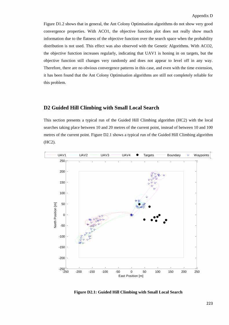
Appendix D
223
Figure D1.2 shows that in general, the Ant Colony Optimisation algorithms do not show very good
convergence properties. With ACO1, the objective function plot does not really show much
information due to the flatness of the objective function over the search space when the probability
distribution is not used. This effect was also observed with the Genetic Algorithms. With ACO2,
the objective function increases regularly, indicating that UAV1 is honing in on targets, but the
objective function still changes very randomly and does not appear to level off in any way.
Therefore, there are no obvious convergence patterns in this case, and even with the time extension,
it has been found that the Ant Colony Optimisation algorithms are still not completely reliable for
this problem.
D2 Guided Hill Climbing with Small Local Search
This section presents a typical run of the Guided Hill Climbing algorithm (HC2) with the local
searches taking place between 10 and 20 metres of the current point, instead of between 10 and 100
metres of the current point. Figure D2.1 shows a typical run of the Guided Hill Climbing algorithm
(HC2).
Figure D2.1: Guided Hill Climbing with Small Local Search
-250 -200 -150 -100 -50 0 50 100 150 200 250-250
-200
-150
-100
-50
0
50
100
150
200
250
East Position [m]
Nort
h P
ositio
n [
m]
UAV1 UAV2 UAV3 UAV4 Targets Boundary Waypoints

Appendix D
224
From Figure D2.1, even with the probability distribution, the local search is too small to guide the
agents to the target areas. Even though there appears to be some movement of the agents in the
correct direction, a larger local search is clearly required if there is to be any chance of the agents
being drawn towards the targets in reasonable time. This justifies expanding the local search to
within 100 metres of the current point.


