Radiometric Sensitivity to Soil Moisture Relative to

Vegetation Canopy Anisotropy, Canopy Temperature,

and Canopy Water Content at 1.4 GHz

by

Brian Kirk Hornbuckle

A dissertation submitted in partial fulfillmentof the requirements for the degree of

Doctor of Philosophy(Electrical Engineering and Atmospheric, Oceanic & Space Sciences)

at The University of Michigan2003

Doctoral Committee:Professor Anthony W. England, ChairProfessor Henry N. PollackAssistant Research Scientist Roger D. De RooProfessor Emeritus Donald J. PortmanProfessor John M. Norman, The University of Wisconsin, Madison

ABSTRACT

Radiometric Sensitivity to Soil Moisture Relative toVegetation Canopy Anisotropy, Canopy Temperature,

and Canopy Water Content at 1.4 GHz

byBrian Kirk Hornbuckle

Chair: Anthony W. England

Many impacts of climate change will be expressed in the hydrologic cycle. Microwave

radiometry is sensitive to the quantity and distribution of water in soil and vegetation. Re-

cent advances in technology will allow global measurements at useful spatial resolutions.

Critical to this vision is the development of reliable models of microwave brightness. In

this dissertation, measurements of 1.4 GHz brightness, micrometeorology, and soil mois-

ture were collected over the course of the growing season in a field of corn. It was de-

termined that the brightness of a field–corn canopy at both polarizations is isotropic in

azimuth during much of the season. At senescence, brightness is a function of row direc-

tion. This phenomenon is caused by water loss from the leaves, which when dry become

essentially invisible. The question is raised whether other biophysical processes associ-

ated with critical periods of drought or extreme wetness could cause similar changes in the

effective constitutive properties of the canopy. A current model of microwave brightness,

appropriate for weakly–scattering canopies, was unable to predict change in brightness with

incidence angle. Significant scatter darkening was observed. A new model was formulated

with an anisotropic canopy. The new model was compared to continuous measurements

of brightness collected during the highest canopy biomass of the season. With the aid of

coincident measurements of micrometeorology and soil moisture, the radiometric sensi-

tivities to vegetation canopy temperature, soil moisture, and canopy water, either in the

form of intercepted precipitation or dew, were determined and compared to sensitivities in

a hypothetical nonscattering canopy of equivalent density, such as thick grass. Sensitiv-

ity to canopy temperature is similar in both types of canopies. Soil moisture sensitivity is

higher in the corn canopy where moisture is concentrated in stems and fruit. An increase in

canopy water has the net effect of decreasing the brightness equally at both polarizations in

corn, while an increase in brightness occurs in nonscattering canopies. Dew can decrease

the brightness more than a soaking rain. With an appropriate emission model, there will be

year round sensitivity to soil moisture in most, and perhaps all, agricultural crops.

ii

c

Brian Kirk Hornbuckle 2003All Rights Reserved

Completed in memory of J. Edwin Nelson and Glen C. Hornbuckle.

I wish I could have shared my joy with you during this process.

Dedicated to Jalene, Amaris, Malachi, and Eliana Hornbuckle.

May our family continue to receive God’s blessings

and share them with others.

ii

ACKNOWLEDGEMENTS

Five people made this work possible.

Mark Fischman built the first 1.4 GHz radiometers.

Roger De Roo made them work in the field.

David Boprie made everything else work.

Tony England found a way to bring all of these people together.

Jason Woods provided an experiment site.

I have been fortunate to have Tony England as my advisor. He allowed me to travel,

to take chances, even at the risk of damaging his reputation, and provided me with inde-

pendence. He has also been a superb mentor and I hope to follow his example of integrity.

Thank you, Tony.

I shared countless hours of field work with David Boprie. Your contribution to the group

has been invaluable. Thank you for watching out for me. I will miss your companionship.

Roger De Roo was always willing to answer any questions. Thank you for sharing your

time with me and others. I thank Don Portman serving on my committee and the significant

amount of time he spent with me in the field and carefully reading my manuscripts. John

Norman added a new dimension to my education after agreeing to serve on my committee

and has become a valuable mentor. I appreciate Henry Pollack’s willingness to join my

committee late in the process.

iii

I can not thank Jason Woods enough for the use of his farm and a remarkable field site.

The quality of the measurements in this work reflect his and his father’s stewardship of their

land. Ned Birkey of Monroe County Extension introduced me to farmers in the area and

kept me involved with agriculture in southeast Michigan. Gerard Kluitenberg at Kansas

State gave instrumentation advice and provided soil texture analysis. Tom Stoffel of the

National Renewable Energy Lab, Tom Kirk of Eppley Lab, Jim Bilskie and Ed Swiatek of

Campbell Scientific, and Sally Logsdon of the Soil Tilth Lab all provided valuable instru-

mentation advice. I would also like to thank Avery Demond for use of her lab in Civil and

Environmental Engineering and Jodi Ryder for her help.

I appreciate the assistance of the following people in the field: David Boprie, Roger

De Roo, Ed Kim, Mark Fischman, Xiaohua Lin, Yuka Muto, Hanh Pham, Ying–Ying

Zhang, Mike Carr, Emily Faivre, Ryan Peterson, Soumitra Ray, Catherine Piowtrowski,

Tarreg Mawari, Aneela Qureshi, Mauricio Vacas, Don Portman, Tony England, and C. E.

Hornbuckle. I appreciate the loan of instruments from Frank Marsik and the Global Change

Laboratory at UM and Tom Jackson of the United States Department of Agriculture.

I would also like to acknowledge the love and support of my parents, Carol and C. E.

Hornbuckle, and Jalene’s parents, Brooksie and Doug Miller.

Finally, I thank my wife Jalene for her love, companionship, affection, and endurance

during this process. I especially am grateful for her determination that I keep my responsi-

bilities as a father throughout the last four and a half years. Because of her hard work, we

are the proud parents of three wonderful children: Amaris, Malachi, and Eliana.

This work was supported by NASA grant NAG5–8661 from the Land Surface Hydrol-

ogy Program. I am grateful for tuition and stipend support provided by an NSF Science

and Engineering Graduate Fellowship, an EPA STAR Graduate Fellowship, a Michigan

Society of Fellows Associate Fellowship, and finally by a Lyman Judson Fellowship from

Rackham Graduate School.

“Thanks Be to God.” Ann Arbor, Michigan, February 6, 2003.

iv

TABLE OF CONTENTS

DEDICATION . . . . . . . . . . . . . . . . . . . . . . . . . . . . . . . . . . . . . ii

ACKNOWLEDGEMENTS . . . . . . . . . . . . . . . . . . . . . . . . . . . . . . iii

LIST OF TABLES . . . . . . . . . . . . . . . . . . . . . . . . . . . . . . . . . . . vii

LIST OF FIGURES . . . . . . . . . . . . . . . . . . . . . . . . . . . . . . . . . . viii

CHAPTERS

1 Climate Variability, Soil Moisture, and Microwave Radiometry . . . . . . 11.1 Introduction . . . . . . . . . . . . . . . . . . . . . . . . . . . . . 11.2 Observed Change in Mean Climate and Climate Variability . . . . 3

1.2.1 Hydrologic Change . . . . . . . . . . . . . . . . . . . . . 31.3 Impacts of Climate Variability . . . . . . . . . . . . . . . . . . . 7

1.3.1 Natural Climate Variability? . . . . . . . . . . . . . . . . 101.4 Soil Moisture and its Effect on Climate . . . . . . . . . . . . . . . 10

1.4.1 Surface Energy Budget . . . . . . . . . . . . . . . . . . . 111.4.2 Predictions of General Circulation Models (GCMs) . . . . 151.4.3 Soil Moisture and Precipitation . . . . . . . . . . . . . . . 171.4.4 Soil Moisture and Extreme Weather . . . . . . . . . . . . 18

1.5 Soil–Vegetation–Atmosphere Transfer . . . . . . . . . . . . . . . 201.6 Microwave Radiometry . . . . . . . . . . . . . . . . . . . . . . . 22

1.6.1 Physical Basis . . . . . . . . . . . . . . . . . . . . . . . . 241.6.2 Brightness Temperature . . . . . . . . . . . . . . . . . . . 251.6.3 Why Microwaves? . . . . . . . . . . . . . . . . . . . . . 261.6.4 Effect of Vegetation . . . . . . . . . . . . . . . . . . . . . 29

1.7 Format of Dissertation . . . . . . . . . . . . . . . . . . . . . . . . 32

2 The Eighth Radiobrightness and Energy Balance Experiment . . . . . . . 332.1 Microwave Radiometers . . . . . . . . . . . . . . . . . . . . . . . 36

2.1.1 Direct–Sampling Digital Radiometer (DSDR) . . . . . . . 372.1.2 DSDR Precision . . . . . . . . . . . . . . . . . . . . . . . 392.1.3 DSDR Calibration . . . . . . . . . . . . . . . . . . . . . . 42

2.2 Laser Profiler . . . . . . . . . . . . . . . . . . . . . . . . . . . . 47

v

2.3 Soil Moisture . . . . . . . . . . . . . . . . . . . . . . . . . . . . 502.3.1 Measurement Technique . . . . . . . . . . . . . . . . . . 512.3.2 Impedance Probe . . . . . . . . . . . . . . . . . . . . . . 542.3.3 Time Domain Reflectometry Instruments . . . . . . . . . . 59

2.4 Micrometeorology . . . . . . . . . . . . . . . . . . . . . . . . . . 672.4.1 Infrared Thermometers . . . . . . . . . . . . . . . . . . . 682.4.2 Soil Temperature . . . . . . . . . . . . . . . . . . . . . . 732.4.3 Summary . . . . . . . . . . . . . . . . . . . . . . . . . . 74

3 The Nature of Absorption, Emission, and Volume Scattering in Field Cornat 1.4 GHz . . . . . . . . . . . . . . . . . . . . . . . . . . . . . . . . . . 76

3.1 Row Anisotropy . . . . . . . . . . . . . . . . . . . . . . . . . . . 763.2 Volume Scattering . . . . . . . . . . . . . . . . . . . . . . . . . . 833.3 Weakly–Scattering Zero–Order Model . . . . . . . . . . . . . . . 923.4 Conclusions . . . . . . . . . . . . . . . . . . . . . . . . . . . . . 94

4 Radiometric Sensitivity to Soil Moisture, Vegetation Temperature, andCanopy Water in Scattering and Nonscattering Canopies at 1.4 GHz . . . . 97

4.1 Model Performance During REBEX–8x3 . . . . . . . . . . . . . . 974.2 Soil Moisture Sensitivity . . . . . . . . . . . . . . . . . . . . . . 1034.3 Dew . . . . . . . . . . . . . . . . . . . . . . . . . . . . . . . . . 1064.4 Intercepted Precipitation . . . . . . . . . . . . . . . . . . . . . . . 1124.5 Conclusions . . . . . . . . . . . . . . . . . . . . . . . . . . . . . 114

5 Summary, Contributions, and Future Work . . . . . . . . . . . . . . . . . 1185.1 Summary . . . . . . . . . . . . . . . . . . . . . . . . . . . . . . 1185.2 Contributions . . . . . . . . . . . . . . . . . . . . . . . . . . . . 1185.3 Future Work . . . . . . . . . . . . . . . . . . . . . . . . . . . . . 121

BIBLIOGRAPHY . . . . . . . . . . . . . . . . . . . . . . . . . . . . . . . . . . . 124

vi

LIST OF TABLES

Table1.1 Likelihood of global changes in climate extremes observed during the twen-

tieth century and predicted for the twenty–first century. From Easterlinget al. [2000b]. . . . . . . . . . . . . . . . . . . . . . . . . . . . . . . . . . 8

2.1 REBEX information. Date information includes days of year. GS refers tovegetation growth stage. H is vegetation height in meters. M is vegetationcolumn density in kg m

2. Mw is water column density in kg m 2. LAI is

leaf area index in m2 m 2. . . . . . . . . . . . . . . . . . . . . . . . . . . 35

2.2 Amplifier temperature variation, σamp, and approximate NE∆T during REBEX–8 and –8x assuming Tsys

400 K. . . . . . . . . . . . . . . . . . . . . . . 412.3 Soil temperature gradients observed during impedance probe measurements. 642.4 Accuracy and precision of instruments used in REBEX–8 and –8x. In some

cases, more than one of the same type of instrument were used to measurea specific variable. For these cases, a second row lists the accuracy andprecision of the averaged data on the plot–scale. . . . . . . . . . . . . . . . 75

3.1 Radiometer footprint size in terms of the number of rows of corn that wouldlie inside of the footprint. Maximum canopy height was 3.0 m. . . . . . . . 80

3.2 Canopy and soil properties during brightness temperature measurements atφ 60

and θ 15

, 35

, and 55

. . . . . . . . . . . . . . . . . . . . . . . 853.3 Values of the volume scattering coefficient, κs in Np m

1, and the single–scattering albedo, α, for a mature field corn canopy. . . . . . . . . . . . . . 92

4.1 Radiometric sensitivity to: vegetation temperature (vt), in K K 1; soil

moisture (sm), in K % 1; and canopy water (cw), in K dg

1 m 2 (Kelvin

per decigram per square meter), for nonscattering canopies, the new zero–order model, and an actual field corn canopy at 1.4 GHz and a water columndensity of 6.3 kg m

2. . . . . . . . . . . . . . . . . . . . . . . . . . . . . 117

vii

LIST OF FIGURES

Figure1.1 Observed linear trends in annual precipitation (% per century) during the

20th century. Green (light) dots indicate increasing trends and brown (dark)dots indicate decreasing trends. From Groisman et al. [2001]. . . . . . . . . 4

1.2 Observed linear trends in total seasonal precipitation and frequency of heavyprecipitation events for various regions of the world during the 20th cen-tury. Natal is in South Africa, Nord–Este is in Brazil. From Easterlinget al. [2000a]. . . . . . . . . . . . . . . . . . . . . . . . . . . . . . . . . . 5

1.3 Impacts of a change in a change in mean (a), a change in variance (b),and a change in both mean and variance (c) on the frequency of extremetemperatures. . . . . . . . . . . . . . . . . . . . . . . . . . . . . . . . . . 7

1.4 Yield (corn for grain) versus year for five southeast Michigan counties:Monroe, Lenawee, Hillsdale, Jackson, and Washtenaw. Yield data obtainedby the author from the Published Estimates Database, United States De-partment of Agriculture (USDA) National Agriculture Statistics Service.Precipitation data used to identify dry months from the National ClimaticData Center. Measurements from the cities of Monroe (Monroe County),Adrian (Lenawee), Hillsdale (Hillsdale), Jackson (Jackson), and Ann Ar-bor (Washtenaw) were used to estimate regional precipitation. Months ofunusually low precipitation are noted. . . . . . . . . . . . . . . . . . . . . 9

1.5 The global hydrologic cycle: flux and storage. Redrawn from Oki [1999]. . 111.6 Mean annual precipitation in mm per day as computed using observations

over a 17-year period (top) and by a GCM. From Koster et al. [2000]. . . . 151.7 Difference in precipitation over the United States between the summer of

1993 and the summer of 1988 [Suarez, Schubert, and Chang, personal com-munication, 2001]. Also cited in Entekhabi et al. [1999]. . . . . . . . . . . 20

1.8 Evaporative fraction (EF) versus soil water index (SWI) for three differentSVAT models each driven with the same data. From Dirmeyer et al. [2000]. 21

1.9 The electromagnetic spectrum. Visible wavelengths lie between the ultra-violet (UV) and the infrared (IR). Drawn by the author. . . . . . . . . . . . 23

viii

1.10 At left, the horizontally– and vertically–polarized brightness temperatureof a smooth bare soil surface as a function of incidence angle for wet anddry soil. At right, an example of a soil moisture map derived from a mapof brightness temperature. . . . . . . . . . . . . . . . . . . . . . . . . . . 27

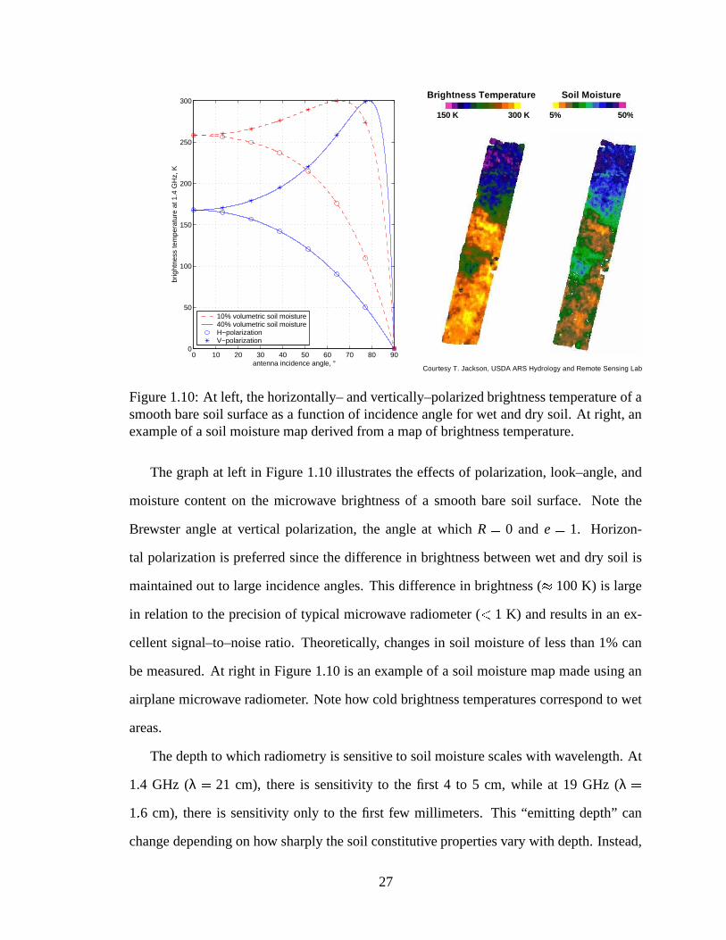
1.11 Modeled brightness temperature as a function of volumetric soil moistureat three different wavelengths, for vegetation column densities of M 1and 4 kg m

2 for an ideal, nonscattering canopy. The soil is treated as auniform halfspace, and soil and vegetation temperature is 295 K. S is thesensitivity of brightness to soil moisture. . . . . . . . . . . . . . . . . . . . 28

1.12 Radiometric sensitivity to vegetation temperature, soil temperature, soilmoisture, and vegetation moisture for an ideal, nonscattering canopy at1.4 GHz. . . . . . . . . . . . . . . . . . . . . . . . . . . . . . . . . . . . . 30

1.13 Anticipated change in 1.4 GHz brightness temperature in response to changesin vegetation temperature (10 K variation in diurnal cycle) and soil mois-ture (desire sensitivity to 4%) in a nonscattering canopy. Expected changein vegetation moisture not known. . . . . . . . . . . . . . . . . . . . . . . 31

2.1 Truck–mounted radiometers and micrometeorological station on day ofyear 144, looking southeast. . . . . . . . . . . . . . . . . . . . . . . . . . 34

2.2 Map of REBEX–8 and –8x site. Truck–mounted radiometers (TMRS) andMicro–meteorological station (MMS) marked. . . . . . . . . . . . . . . . . 36

2.3 Amplifier and reference load temperatures for the V–pol DSDR duringREBEX–8x3. . . . . . . . . . . . . . . . . . . . . . . . . . . . . . . . . . 41

2.4 An example of radiometer precision during REBEX–8x4. Soil and vegeta-tion temperatures and soil moisture (not shown) were essentially constantduring the 20–minute period between 7:40 and 8:00 Local Daylight Time(LDT). Presented NE∆T is for the 10 brightness temperature measurementsmade during this period. . . . . . . . . . . . . . . . . . . . . . . . . . . . 42

2.5 At left: absorber calibration. At right: microwave absorber. . . . . . . . . . 432.6 DSDR calibration procedure. . . . . . . . . . . . . . . . . . . . . . . . . . 452.7 Recorded reference load rQ and fitted polynomial for the H–pol DSDR

during REBEX–8x3. . . . . . . . . . . . . . . . . . . . . . . . . . . . . . 462.8 Laser profiler. . . . . . . . . . . . . . . . . . . . . . . . . . . . . . . . . . 472.9 Two examples of recorded soil surface profile. . . . . . . . . . . . . . . . . 482.10 Computed correlation function. . . . . . . . . . . . . . . . . . . . . . . . . 492.11 Soil topography during REBEX–8 and REBEX–8x reduced to a binary

representation. . . . . . . . . . . . . . . . . . . . . . . . . . . . . . . . . . 512.12 TDR during REBEX–8: at left, in a high area at 1.5 cm; at right, in a low

area at 4.5 cm. . . . . . . . . . . . . . . . . . . . . . . . . . . . . . . . . . 522.13 Impedance probe. Each of the four tines are 6 cm long. . . . . . . . . . . . 522.14 Orientation of impedance probe and TDR. Top: side view. Bottom: plan

view. Drawn to scale. . . . . . . . . . . . . . . . . . . . . . . . . . . . . . 532.15 Equipment used to measure gravimetric water content (at left) and bulk

density (at right). . . . . . . . . . . . . . . . . . . . . . . . . . . . . . . . 56

ix

2.16 Histograms of cup mass before (at left) and after (at right) drying in a105

C oven. . . . . . . . . . . . . . . . . . . . . . . . . . . . . . . . . . 572.17 Impedance probe calibration. . . . . . . . . . . . . . . . . . . . . . . . . . 582.18 The index of refraction of pure water (σe

0) at 305 K and 275 K. . . . . . 602.19 Proposed WCR period temperature correction based on Seyfried and Mur-

dock [2001]. . . . . . . . . . . . . . . . . . . . . . . . . . . . . . . . . . . 622.20 TDR calibration. . . . . . . . . . . . . . . . . . . . . . . . . . . . . . . . 632.21 Solar radiation, precipitation, soil temperature at 1.5 cm, and 0–3 cm soil

moisture in H areas during REBEX–8. Local Daylight Time. . . . . . . . . 652.22 Comparison of 0–6 cm volumetric soil water content measured by the

ThetaProbe with the average of 0–3 cm and 3–6 cm volumetric soil wa-ter content measured by the Water Content Reflectometers. . . . . . . . . . 66

2.23 Spectral irradiance of a clear sky of effective temperature Tsky 288 K

within the band of the IR thermometer. Approximated from Figure 10.6 ofCampbell and Norman [1998]. Blackbody irradiance is also plotted. . . . . 71

2.24 Radiometric temperature reported by an IR thermometer as a function ofincident radiance. . . . . . . . . . . . . . . . . . . . . . . . . . . . . . . . 72

3.1 Truck–mounted radiometers on day of year 178. Antennae oriented atθ 35

φ 60

. Micro–meteorological station tower can be seen in thebackground. . . . . . . . . . . . . . . . . . . . . . . . . . . . . . . . . . . 77

3.2 Time sequence of H–pol and V–pol brightness temperature as a functionof angle with respect to row direction (φ) during REBEX–8x3. Errorbarsof

NE∆T are included. The measurements at φ 60

and θ 35

arecircled. Soil temperature at 1.5 cm and vegetation IR temperature are alsoplotted. . . . . . . . . . . . . . . . . . . . . . . . . . . . . . . . . . . . . 78

3.3 Measurement procedure during REBEX–8x3. . . . . . . . . . . . . . . . . 793.4 Change in V–pol brightness temperature from φ 60

as a function ofangle with respect to row direction during REBEX–8x1, –8x3, –8x3, and–8x4. The size of the markers on the data are approximately the same sizeas

NE∆T and therefore errorbars are not included. . . . . . . . . . . . . . 81

3.5 Change in H–pol brightness temperature from φ 60

as a function ofangle with respect to row direction during REBEX–8x3 and –8x4. Error-bars on the REBEX–8x4 data are

NE∆T. The size of the markers on the

REBEX–8x3 data are approximately the same size as

NE∆T and there-fore errorbars are not included. . . . . . . . . . . . . . . . . . . . . . . . . 82

3.6 Distribution of water column density during each REBEX. . . . . . . . . . 833.7 Observed (a) and modeled (b, c, and d) H–pol brightness temperature at

φ 60

during REBEX–8, –8x3, and –8x4. For the model results: (b),the soil surface is specular; (c), the soil surface is rough; and (d), the soilsurface is rough and α 0. . . . . . . . . . . . . . . . . . . . . . . . . . . 87

x

3.8 Observed (a) and modeled (b, c, d, and e) V–pol brightness temperature atφ 60

during REBEX–8x1, –8x2, –8x3, and –8x4. For the model results:(b), the soil surface is specular; (c), the soil surface is rough; (d), the soilsurface is rough and R is not a function of θ; and (e), the soil surface isrough, R is not a function of θ, and α 0. . . . . . . . . . . . . . . . . . . 90

3.9 Volume scattering coefficients, κs (top), and extinction coefficients, κe (bot-tom), versus incidence angle. . . . . . . . . . . . . . . . . . . . . . . . . . 94

4.1 Precipitation, soil moisture, vegetation and soil temperatures, and 1.4 GHzbrightness temperature (θ 35

, φ 60

) during REBEX–8x3. . . . . . . 984.2 Precipitation and soil moisture leading up to REBEX–8x3. . . . . . . . . . 1004.3 Observed and modeled H– and V–pol brightness temperatures during REBEX–

8x3. . . . . . . . . . . . . . . . . . . . . . . . . . . . . . . . . . . . . . . 1014.4 Soil moisture at 0–3 cm and the difference between V–pol and H–pol bright-

ness temperatures during REBEX–8x3. . . . . . . . . . . . . . . . . . . . 1044.5 Modeled brightness temperature of the soil, just below the vegetation canopy,

during REBEX–8x3. . . . . . . . . . . . . . . . . . . . . . . . . . . . . . 1054.6 Soil moisture at 0–3 cm and the difference between V–pol and H–pol bright-

ness temperatures during REBEX–8x3. . . . . . . . . . . . . . . . . . . . 1064.7 Canopy temperature, modeled dew deposition to the canopy, and H– and

V–pol brightness temperatures during the night for days 228/229 and 229/230.1094.8 Air temperature at 7.8 m, wind speed at 10 m, and dew point temperature

at 7.8 m for the night of days 228/229 (top) and the night of days 229/230(bottom). . . . . . . . . . . . . . . . . . . . . . . . . . . . . . . . . . . . 111

4.9 Modeled and measured sensitivity of H–pol 1.4 GHz brightness tempera-ture to volumetric soil moisture in field corn. . . . . . . . . . . . . . . . . . 115

4.10 Anticipated change in H–pol brightness temperature in response to typi-cal changes in vegetation temperature, soil moisture, and canopy water at1.4 GHz for a real (scattering) mature field corn canopy and an equivalentnonscattering canopy . . . . . . . . . . . . . . . . . . . . . . . . . . . . . 116

xi

CHAPTER 1

Climate Variability, Soil Moisture, and MicrowaveRadiometry

1.1 Introduction

To what degree is climate changing in response to human activities?

What would be the impacts of any climate change?

What amount of natural climate variability can be expected?

We can answer these important questions now with some certainty. There has been

significant warming over the past century in the observational record [Intergovernmental

Panel on Climate Change, 1996] and the twentieth century was the warmest of the past

five centuries [Pollack et al., 1998]. Losses in weather catastrophes have increased steadily

over the past fifty years, due to both an increase in the frequency of catastrophes and to

shifts in land use, a sign of society’s increasing susceptibility to extreme weather [Kunkel

et al., 1999b]. To separate anthropogenic effects from naturally occurring variability, we

must continue to develop our understanding of Earth’s climate. One important process

that is still not well understood is the exchange of water between the soil, vegetation, and

atmosphere.

“Water is at the heart of climate change and the impacts of climate variabil-

ity. Any assessment of climate change, its causes and impacts, must be based

1

on significantly better observations of the water cycle.” [National Research

Council, 1999]

Microwave radiometry, the measurement of naturally emitted microwave radiation, is

sensitive to the presence of liquid water. When directed toward the earth’s surface, it can

reveal the the quantity and distribution of water stored in vegetation and the first few cen-

timeters of the soil, key components of the water cycle. Although the response to changes

in soil water content has been well documented, there are still many questions about the

effect of the overlying vegetation. For example:

Can scattering of radiation within the vegetation canopy be neglected? The most

widely used model for land surface microwave brightness assumes negligible scatter-

ing, but it has been validated only at steep angles of incidence at which the vegetation

has the least impact.

At what level of vegetation is there no longer any useful sensitivity to changes in soil

water content? Does the transparency of the canopy depend on simply the amount of

water in the canopy or also on its distribution?

What effect do changes in vegetation water content have upon the emitted microwave

radiation? These variations can be caused by intercepted precipitation and dew, or

by slower, more subtle processes such as diurnal variations, senescence, and plant

response to drought or extreme wetness.

In this dissertation, I first examine the electromagnetic properties of one type of veg-

etation canopy, field corn, and show that if scattering is neglected, the canopy must be

considered an anisotropic medium. I then formulate a new model which assumes weak

scattering. Finally, I quantify the effect of changes in vegetation temperature, soil mois-

ture, and the amount and distribution of moisture within a corn canopy on the microwave

brightness, and compare these effects with those which would be observed in a hypothetical

nonscattering canopy such as thick grass by comparing the new model with observations.

2

Both the European Space Agency and NASA have plans to launch satellite microwave

radiometers later this decade. These new instruments, in conjunction with the findings of

this dissertation and other ongoing research, will allow us to further our understanding of

the climate system and, in the future, to intelligently manage humanity’s impact on Earth’s

climate and environment.

1.2 Observed Change in Mean Climate and Climate Vari-ability

An increase of 0.6

C in the global mean temperature record since the beginning of the

20th century has been observed [Intergovernmental Panel on Climate Change, 1996]. Us-

ing data from 358 boreholes in eastern North America, central Europe, southern Africa,

and Australia, Pollack et al. [1998] concluded that the average surface temperature has in-

creased 0.5

C in the 20th century and that the 20th century is the warmest of past five cen-

turies. Furthermore, a greater warming in daily minimum temperature than daily maximum

temperature has been observed [Easterling et al., 1997]. Not only have mean temperatures

increased in the past century, it also appears that they have become more variable. In the

United States, for example, the two–month period of November and December, 2000, was

the coldest such period on record. This followed the warmest winter on record, and the

January through October, 2000, period was the warmest 10–month period since records

began in 1895. The ten warmest years on record have all occurred since 1983 [News and

Notes, 2001].

1.2.1 Hydrologic Change

Besides changes in temperature during the past century, changes in Earth’s hydrology

have also been observed. The areas of the world affected by drought or excessive wetness

has increased overall, although there is significant local variability. In the United States,

excessive wetness is increasing, while in China, an increase in the areas affected by drought

3

Figure 1.1: Observed linear trends in annual precipitation (% per century) during the 20thcentury. Green (light) dots indicate increasing trends and brown (dark) dots indicate de-creasing trends. From Groisman et al. [2001].

has been observed [Easterling et al., 2000b]. Both an overall increase in annual precipita-

tion (Figure 1.1) and an increase in heavy precipitation events have been observed in the

United States [Karl et al., 1996; Karl and Knight, 1998; Kunkel et al., 1999a; Groisman

et al., 1999, 2001].

Changes in precipitation amount and frequency have also been observed worldwide.

Figure 1.2 shows trends in total seasonal precipitation and the frequency of heavy precipi-

tation within that season for various regions of the world during the past century. For each

region (e.g. USA, W. USSR, etc.) the season with the maximum precipitation was selected.

For the United States, this season is the summer (the months of June, July, and August).

The frequency of heavy precipitation is found by counting the number of days the precip-

itation exceeds a region–specific threshold within that season. The thresholds range from

20 mm to 100 mm. The total length of time analyzed for each region ranges from 34 to 96

4

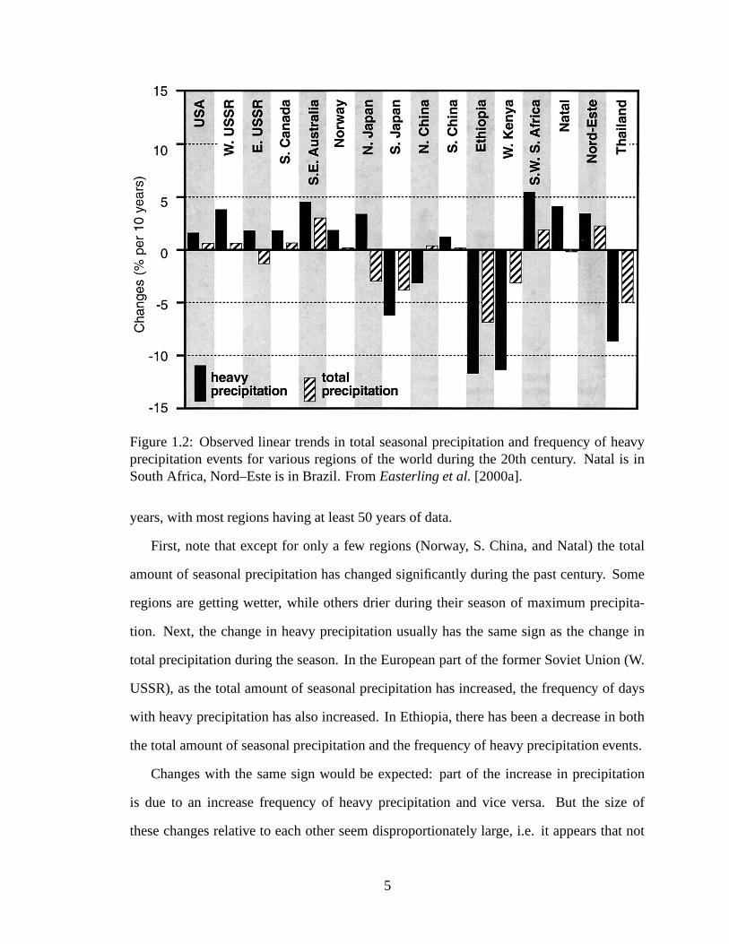
Figure 1.2: Observed linear trends in total seasonal precipitation and frequency of heavyprecipitation events for various regions of the world during the 20th century. Natal is inSouth Africa, Nord–Este is in Brazil. From Easterling et al. [2000a].

years, with most regions having at least 50 years of data.

First, note that except for only a few regions (Norway, S. China, and Natal) the total

amount of seasonal precipitation has changed significantly during the past century. Some

regions are getting wetter, while others drier during their season of maximum precipita-

tion. Next, the change in heavy precipitation usually has the same sign as the change in

total precipitation during the season. In the European part of the former Soviet Union (W.

USSR), as the total amount of seasonal precipitation has increased, the frequency of days

with heavy precipitation has also increased. In Ethiopia, there has been a decrease in both

the total amount of seasonal precipitation and the frequency of heavy precipitation events.

Changes with the same sign would be expected: part of the increase in precipitation

is due to an increase frequency of heavy precipitation and vice versa. But the size of

these changes relative to each other seem disproportionately large, i.e. it appears that not

5

only is the frequency of heavy precipitation increasing as a result of the overall increase

in precipitation, but the manner in which precipitation falls, either in light or heavy rain

events (the variability of precipitation) is also changing. Although it is tempting to make

this strong generalization, it can not be made solely on this information in all cases. On

the other hand, in four regions (E. USSR, N. Japan, N. China, and Natal) the changes have

opposite signs. In these regions, we can say with confidence that not only is the mean

amount of seasonal precipitation changing, so is the variability. For example, there has

been an increase in the frequency of heavy precipitation in N. Japan despite the fact that

the overall amount has decreased.

Besides changes in precipitation, changes in streamflow data have also been observed.

Lins and Slack [1999] analyzed streamflow data from the Hydro-Climatic Data Network

(HCDN), a network of over 1500 stream gauges across the United States. Using a subset of

these data consisting of stations with daily records over long periods of time, they found that

annual low and median daily mean discharge rates have increased during the 20th century.

Interestingly, the maximum average daily streamflow during each year had not increased

significantly. Groisman et al. [2001] analyzed the same data set in order to discover why an

increase in heavy precipitation events was apparently not causing an increase in maximum

streamflow. After eliminating data from the Western United States, where snow melt can

mask the effect of precipitation on streamflow, they found that in the Eastern United States

there has been an increase in high streamflow during the month of maximum streamflow in

response to the increase in heavy precipitation.

Douglas et al. [2000] also analyzed the HCDN streamflow data. They used a special sta-

tistical method designed to discount any significance resulting from correlated streamflow

within the same basin. For example, if the streamflow at an up–river gauge is high, then

naturally the streamflow downstream would also tend to be high. Their method included

only one of these gauges in their analysis. Over a fifty year period from 1939 to 1988,

no statistically significant increase in flood flows (the maximum average daily streamflow

6

freq

uenc

y

a

temperature

b c

Figure 1.3: Impacts of a change in a change in mean (a), a change in variance (b), and achange in both mean and variance (c) on the frequency of extreme temperatures.

during each water year, October through September) were found at any time or space scale.

However, an increase in the level of low flows (the lowest seven-day average streamflow

during each drought year, April through March) was found in the Upper Midwest over the

past fifty years.

1.3 Impacts of Climate Variability

Changes in Earth’s climate may affect both mean values and the frequency of extreme

events. For example, a single increase in mean daily maximum temperature may also in-

crease the frequency of extreme high temperatures (plot a in Figure 1.3). If instead mean

daily maximum temperatures do not change, a change in the variance, or spread, of the

temperature distribution would also increase the frequency of extreme temperatures (plot b

in Figure 1.3). A change in both mean and variance (plot c in Figure 1.3) would result in a

much larger frequency of extreme temperatures than changes in mean or variance by them-

selves [Meehl et al., 2000]. Although a general warming in the earth’s climate is a concern,

it is likely that humans can adapt to slow changes in mean temperature. On the other hand,

we are much more sensitive to extreme weather events, part of the climate variability. An

increase in extreme events such as heat waves, cold snaps, droughts, and floods could have

7

Table 1.1: Likelihood of global changes in climate extremes observed during the twentiethcentury and predicted for the twenty–first century. From Easterling et al. [2000b].

Observed (20th Century) Predicted (21st Century)higher maximum temperatures very likely very likelymore hot summer days likely very likelyincrease in heat index likely very likelymore heat waves possible very likelyhigher minimum temperatures virtually certain very likelyfewer frost days virtually certain likelyfewer cold waves very likely very likelymore heavy one–day precip events likely very likelymore heavy multi–day precip events likely very likelymore drought likely very likelymore wet spells likely likelymore intense mid–latitude storms possible possible

devastating effects [Kunkel et al., 1999b]. Not only should we be concerned with mean

changes in temperature and precipitation, but also with how the variability of temperature

and precipitation may be changing (Table 1.1).

One example of our susceptibility to climate variability is agriculture. Figure 1.4 is a

graph of field corn yield versus year for five counties in Southeast Michigan since 1955.

Note that although agricultural production has increased over the years, productivity is still

limited by weather, in particular precipitation. Each dip in yield is associated with ab-

normally dry months during the growing season. The amount, timing, and seasonality of

precipitation are all important [Sharratt et al., 2001]. Both surface water (the moisture im-

mediately replenished by precipitation) and groundwater (recharged slowly over the entire

year) supply moisture to growing vegetation. For corn, during May and June the plant roots

are too shallow to reach moisture well below the surface and hence depend on a pattern of

precipitation that sufficiently wets the surface. By the middle of the summer, the amount of

water lost through evapotranspiration outweighs the amount moisture in the form of precip-

itation, and the roots of the corn plant must pull moisture from deeper depths in the ground,

moisture that was deposited during the preseason in the late fall, winter, and early spring.

8

1955 1960 1965 1970 1975 1980 1985 1990 1995 200050

60

70

80

90

100

110

120

year

yiel

d, b

ushe

ls a

cre−

1

Field Corn Production in Five SE Michigan Counties

Unusually Dry Months Noted

Jul,Aug

May,Jun

Jun−Aug

Jul,Aug

Jun,Jul

Mar,Aug

Apr,May,Aug

Jul,Aug

Jul,Aug

Apr−Aug

Jul

Figure 1.4: Yield (corn for grain) versus year for five southeast Michigan counties: Monroe,Lenawee, Hillsdale, Jackson, and Washtenaw. Yield data obtained by the author from thePublished Estimates Database, United States Department of Agriculture (USDA) NationalAgriculture Statistics Service. Precipitation data used to identify dry months from theNational Climatic Data Center. Measurements from the cities of Monroe (Monroe County),Adrian (Lenawee), Hillsdale (Hillsdale), Jackson (Jackson), and Ann Arbor (Washtenaw)were used to estimate regional precipitation. Months of unusually low precipitation arenoted.

In most parts of the Corn Belt, the ground water moisture supply is almost always present

and precipitation during the growing season is the limiting factor. On the western edge of

the Corn Belt where annual rainfall is lower, this is not always the case. Neild et al. [1987]

analyzed corn yields and precipitation data in Eastern Nebraska for dry–land (as opposed

to irrigated) fields. When preseason (September to May) precipitation was above average,

there was a 70% probability that corn yields would be above average also, regardless of

what happened during the rest of the growing season.

Although a farmer must be able to survive occasional poor growing years, any increase

in the variability of precipitation could disrupt this delicate balance and be economically

disastrous to the agricultural community. Our world as a whole is becoming more sensitive

9

to climate variability. Losses in weather catastrophes have increased steadily over the past

fifty years, mainly due to shifts in land use (a greater susceptibility to extreme weather such

as hurricanes and floods) and not just an increased frequency in the number of catastrophes

[Kunkel et al., 1999b].

1.3.1 Natural Climate Variability?

Despite the fact that the phrase “climate change” has only recently become part of our

everyday language, there have always been varying amounts of climate change in Earth’s

history. Since the Industrial Revolution, humans have had an increasingly stronger impact

on the environment and climate. Although increased concentrations of greenhouse gases in

the atmosphere from the combustion of fossil fuels lead scientists to believe that the climate

variability observed in the past century is not part of the natural climate variability, they

have yet to determine exactly how climate has been affected. The ability to answer this

question is limited by the finite (and relatively short) length of the observational record and

by incomplete knowledge of the processes which determine Earth’s climate.

Further study of the climate system will allow a better characterization of the climate

we will experience in the future. In the meantime, it is only prudent to encourage the use

of alternative sources of energy [Hoffert et al., 2002] to avoid further compounding the

problem. Otherwise we may consign ourselves to many negative consequences such as

hotter and drier summers, the expansion of arid areas, drought in the tropics, and flooding

in high– and mid–latitude rivers [Wetherald and Manabe, 2002].

1.4 Soil Moisture and its Effect on Climate

One important process that is not well understood is the cycling of water between the

Earth’s surface and atmosphere. Water is continuously exchanged between the oceans,

atmosphere, and land surface in a process known as the hydrologic cycle. Figure 1.5 illus-

trates the the dominant exchange mechanisms and storage areas of water on the Earth and

10

atmospheric water vapor over

oceans = 10

atmospheric water vapor

over land = 3

water vapor flux = 40

precipitation = 391

evaporation = 431

oceans = 1,338,000

runoff = 40

precipitation = 115

evapotranspiration = 75glaciers, snow = 24,064

biomass = 1

permafrost = 300

soil moisture = 17ground water = 23,400

lakes = 176 marshes = 11rivers = 2

state variable: amount of water in 1015 kg f lux: amount of water in 1015 kg per year

Figure 1.5: The global hydrologic cycle: flux and storage. Redrawn from Oki [1999].

their magnitude. The amount of water stored in the unsaturated zone of the Earth’s surface

above the water table is commonly referred to as soil moisture. Although the soil stores

little water relative to other reservoirs, it receives the majority of the water returned to the

surface via precipitation and is a major source of water for evaporation and transpiration.

As a result, soil moisture is a very active reservoir unlike the other larger, essentially static

reservoirs.

1.4.1 Surface Energy Budget

A more quantitative analysis of the role of soil moisture in the climate system can

also be seen by examining the energy budget at the Earth’s surface. The total amount of

radiative energy per unit area per second directed towards the Earth’s surface is the sum

of the incident solar radiation, S, and emission from the atmosphere, A. Some of the solar

radiation is reflected and the surface also emits radiation. The net radiation can be written

[Arya, 1988]:

Rn S A

aS eσT 4s (1.1)

11

Here a is the albedo, σ is the Stefan–Boltzmann constant, e the emissivity, and Ts is the

surface temperature. During the night, the net radiation is usually negative, but during

the day it reaches several hundred W m 2. By conservation of energy, the net radiation

is balanced by sensible heat flux into the atmosphere, HS; the flux of latent heat into the

atmosphere, HL; the flux of heat into the ground, G; and the rate of change of energy stored

in the vegetation canopy (if present), Wveg:

Rn HS HL G Wveg (1.2)

HS is primarily the convection (including conduction) of heat away from the surface. It is

dependent on both the temperature difference between the surface and the atmosphere and

the degree and nature of turbulence. Both G and Wveg are normally small when integrated

over the course of a day.

Just as the human body perspires to cool itself when hot, so too “sweat” soil and veg-

etation when warmed by the sun. Accordingly, latent heat flux is equal to the rate of

evaporation and transpiration, E, multiplied by the latent heat of vaporization, Le:

HL Le E (1.3)

Soil moisture is the source of most water evaporated from the soil and transpired by plants.

In heavily vegetated areas, the evapotranspiration can be relatively large. For example, on

a single day in the middle of August, 23,540 liters (6218 gallons) of water per acre were

removed from the soil in a field of corn near Britton, Michigan, largely from transpiration

but also by evaporation from the bare soil beneath the canopy [personal data, 1999]. In

comparison, 25 mm (one inch) of rain on one acre of ground is equivalent to 102,900 liters

(27,200 gallons) of water. During the height of the growing season in mid–August, this

crop was removing the equivalent of more than an inch of rain from the soil every five days.

In a single day, a hundred–acre field loses an amount of water equivalent to an Olympic–

sized swimming pool. For a sense of the amount of latent heat transferred, imagine the

energy required to boil the water of this swimming pool.

12

Eltahir [1998] outlined the details of a possible soil moisture – rainfall positive feed-

back. In general, wet soil increases net radiation, total heat flux into the atmospheric bound-

ary layer (the layer of air directly influenced by the Earth’s surface), and the moist static

energy, Wmse, within the boundary layer. The moist static energy of an air parcel per unit

mass is the sum of its potential energy, thermal energy, and latent heat stored by water

vapor:

Wmse gz cpT Leq (1.4)

where g is the acceleration of gravity, z the elevation of the air parcel, cp the air specific

heat, T the temperature, and q the specific humidity. Wmse has units of energy per unit mass.

There are two main pathways through which soil moisture can enhance the likelihood

of precipitation, which in turn raises the soil moisture and enhances precipitation.

1. Wet soil absorbs more solar radiation because of its lower albedo, which results in

an increase in daytime Rn at the surface. This leads to a greater flux of energy into

the boundary layer according to (1.2), which increases Wmse. An increase in Wmse

strengthens both: the vertical gradient of Wmse in atmosphere, making convection

and subsequent precipitation more likely; and the horizontal gradient of Wmse, en-

hancing atmospheric circulation and the movement of atmospheric moisture from

other areas into the region. Furthermore, a higher Wmse brings the elevation at which

water condenses in the boundary layer closer to the surface, increasing the likelihood

of precipitation from convection.

2. Wet soil increases HL which increases the total flux of energy and water vapor to

the boundary layer and decreases the surface temperature. The decrease in surface

temperature increases net radiation at surface according to (1.1), which leads to an

increased probability of precipitation as detailed in the first pathway. The decrease in

surface temperature also decreases the amount by which the air must cool in order to

saturate (lowers the wet bulb depression) which allows clouds to form closer to the

13

surface and decreases the boundary layer depth. Given the same amount of HS and

HL, Wmse is larger in a smaller boundary layer.

Eltahir [1998] supported this theoretical framework with data from the First Interna-

tional Satellite Land Surface Climatology Project (ISLSCP) Field Experiment (FIFE) in

Kansas. Using soil moisture and precipitation records in Illinois, Findell and Eltahir [1997]

found a small but statistically significant positive correlation between soil moisture and

subsequent rainfall in Illinois. In a later paper, Findell and Eltahir [1999] used soil mois-

ture and near surface observations of air temperature, humidity, and pressure in Illinois to

further analyze soil moisture – rainfall feedback. They found that this feedback was not

due to a positive correlation between soil moisture and boundary layer moist static energy,

nor was there a positive correlation between moist static energy and precipitation. On the

other hand, the theoretical relationship between soil moisture and wet bulb depression, and

between wet bulb depression and subsequent rainfall did hold true.

Recently, Findell [2001] determined that a more complete analysis of the structure and

composition of the boundary layer is needed to determine the relationship between soil

moisture and precipitation. In particular, the moisture content of the air in the lower tro-

posphere and the early morning temperature gradient between 1 and 3 km have a great

influence on the likelihood of convection and subsequent rainfall. Using data from Illinois

and a boundary layer model, she found that when the air is very moist, surface fluxes have

little effect and the likelihood of precipitation is atmospherically controlled. The same is

true for very dry air. Between these two extremes, the existence of a temperature inver-

sion (virtual temperature increases with height) in the critical region inhibits convection.

When there is a near dry adiabatic lapse rate (10 K km 1), dry soils are more likely to in-

duce convection, i.e. there is a negative feedback between soil moisture and precipitation.

The dry adiabatic lapse rate is the rate at which dry air cools with elevation assuming no

exchange of heat between an air parcel and the surrounding atmosphere. When the lapse

rate is close to moist adiabatic, wet soils are more likely to induce precipitation (a positive

14

Figure 1.6: Mean annual precipitation in mm per day as computed using observations overa 17-year period (top) and by a GCM. From Koster et al. [2000].

feedback). The moist adiabatic lapse rate is the rate at which saturated air cools with ele-

vation. It is always less than the dry adiabatic lapse rate because of release of latent heat

with condensation.

1.4.2 Predictions of General Circulation Models (GCMs)

The relationship between soil moisture and precipitation, as well as the general role

of soil moisture in the climate system, has also been examined using atmospheric General

Circulation Models (GCMs), complex numerical models that simulate the behavior of the

atmosphere on large scales. GCMs can not perfectly reproduce Earth’s climate, but they

15

are still extremely useful for two reasons. First, model predictions have been verified with

actual observations in a qualitative sense. Figure 1.6 shows mean annual precipitation

in mm per day as computed using observations over a 17-year period and by the NASA

Goddard Earth Observing System-Climate (GEOS-ARIES) GCM with 720 years of forcing

data. Note that the model reproduces the general qualities of observed precipitation, i.e.

regions which are dry match the regions predicted to be dry, but the match is not perfect.

For example, the Sahara Desert is easy to see in the model output, but it is too dry. Second,

GCMs produce physically intuitive results. When high levels of carbon dioxide, methane,

and other greenhouse gases occur in the atmosphere, GCMs correctly produce a warming

of climate and an intensification of the water cycle [Washington, 1992].

Many researchers have used GCMs to investigate soil moisture’s effect on climate.

Manabe [1969] was able to reproduce the qualitative features of global water and energy

cycle after incorporating the effect of land surface hydrology into one of the first GCMs.

Walker and Rowntree [1977] found that when a desert area was replaced by moist land

in a GCM, wetness was maintained for several weeks. This led them to conclude that

ground dryness sustain desert conditions and that soil moisture is important both in short–

range forecasts (one to two days) and over longer periods of time (more than 2 weeks).

Mahfouf [1991] and Mintz and Walker [1993] both used GCM studies to illustrate the

intricate relationship between soil moisture, evapotranspiration, and energy transfer at the

Earth’s surface. Delworth and Manabe [1989] compared a 50–year GCM simulation where

soil moisture was free to change with a 50–year simulation where soil moisture was pre-

scribed and verified that interactive soil moisture was directly connected to the fluctuations

of near–surface relative humidity and temperature and increased the total variability of the

atmosphere. Segal and Arritt [1992] found that a thermally–induced circulation equivalent

in intensity to a sea breeze can be caused by sharp contrast between extended wet soil or

crops and adjacent dry land areas.

16

1.4.3 Soil Moisture and Precipitation

A relationship between soil moisture and precipitation has been noted by other re-

searchers in GCM studies. Shukla and Mintz [1982] found that rainfall, atmospheric mo-

tion, and temperature depend strongly on land surface evapotranspiration and that vegeta-

tion plays an important role in climate. Rind [1982] reduced soil moisture to 25% of its

observed value, found that subsequent summertime temperatures are higher and precipita-

tion decreases, and concluded that knowledge of late spring soil moisture can help predict

summertime precipitation. Yeh et al. [1984] found that irrigation affected the distribution

of evaporation and precipitation and that anomalies of soil moisture persisted for several

months due to positive feedback between increased evaporation and precipitation. Oglesby

and Erickson [1989] concluded that reduced soil moisture can prolong and amplify North

American drought. Koster and Suarez [1996] found that shortening the soil water reten-

tion period resulted in increased precipitation variance. Bonan and Stillwell-Soller [1998]

concluded that soil moisture feedbacks amplified the severity and persistence of floods and

droughts in the Mississippi River Basin.

Beljaars and Viterbo [1999] emphasized the importance of the land surface by illustrat-

ing the improvement in precipitation forecasts in the European Center for Medium–range

Weather Forecasting’s (ECMWF) GCM when modeling of land–atmosphere interaction

was improved. Koster et al. [2000] found that land–atmosphere feedback can amplify or

suppress the chaotic nature of the atmosphere. Knowledge of the land surface state im-

proved precipitation predictability in “transition” regions between very humid and very

dry areas, typically over the middle of large continents, where there is sufficient energy to

evaporate surface water and surface water is variable. On the other hand, knowledge of

sea surface temperature (SST) is more useful at higher latitudes where net radiation is low,

and in deserts and very humid and wet areas. Hong and Pan [2000] observed strong posi-

tive feedback between soil moisture and precipitation due mostly to the effect on turbulent

mixing than the input of moisture into atmosphere. Hong and Kalnay [2000] simulated

17

the Oklahoma–Texas drought of 1998 and found that SST anomalies and favorable initial

conditions established the drought in the late spring and that the drought was maintained

by positive feedback from dry soil moisture conditions during the summer. The drought

ended in the fall when stronger large–scale weather systems overwhelmed the soil moisture

positive feedback. They also emphasized that when appropriate physical models of land–

atmosphere interaction are incorporated into GCMs, forecasting skill will greatly increase.

1.4.4 Soil Moisture and Extreme Weather

Researchers have also used GCMs retrospectively to study extreme weather events.

Chang and Wetzel [1991] simulated the development of a tornado that occurred during rel-

atively quiet atmospheric conditions near Grand Island, Nebraska. They compared three

different GCM simulations: no spatial variation of soil moisture or vegetation; soil mois-

ture variation; and soil and vegetation variation. Realistic soil moisture and vegetation

variations produced the best forecast and they noted that the “observed stationary front was

strongly enhanced by differential heating caused by observed gradients of soil moisture, as

acted upon by the vegetation cover.”

Pan et al. [1995] found that artificially adding moisture to soil in a GCM simulating

the record Midwest drought of 1988 changed relative precipitation but did not create any

new areas of precipitation and concluded that a sudden increase in soil moisture would not

have stopped the drought. When simulating the record Midwest floods of 1993 they found

that the saturated surface significantly contributed to the total rainfall. Their conclusion

was that local recycling of water is more important during times of extreme wetness than

during drought. On the other hand, Giorgi et al. [1996] concluded that local recycling of

evaporated water was not important as compared to large scale moisture fluxes and synoptic

activity during the drought of 1988 and the floods of 1993. Furthermore, they found that

the main effect of decreased evaporation is to increase buoyancy and sustain convection. In

other words, there is a negative feedback between soil moisture and precipitation. Trenberth

18

and Guillemot [1996] postulated that although the 1988 drought and 1993 floods were

initiated by large scale sea surface temperature and atmospheric circulation anomalies (La

Nina in 1988, El Nino in 1993), soil moisture acted to amplify and prolong the wet and dry

conditions. In contrast to Pan et al. [1995], Dirmeyer and Brubaker [1999] examined the

transport and surface sources of moisture supplying precipitation over the United States

during the drought of 1988 and floods of 1993 and found that 41% of the precipitation

in the Mississippi River Basin originated locally in 1988 compare to only 33% in 1993.

During the peak of flooding in July 1993, the precipitation – soil moisture recycling ratio

was considerably lower than other months that year. The main source of moisture was

the Gulf of Mexico and Caribbean. In 1988, during the peak of the drought in June the

recycling ratio was maximum, implying that soil moisture played an important role in the

persistence of the drought.

From these studies it is clear that soil moisture has a significant effect on climate, al-

though the exact nature of its effect has yet to be determined. Figure 1.7 graphically illus-

trates the effect current soil moisture (SM) conditions have on the weather predictions of

one particular model, the NASA Goddard GCM [personal communication, Suarez et al.,

2001] and [Entekhabi et al., 1999]. Map A displays the observed difference in precipitation

over the United States during the summer of 1993 (the record flood year in the Midwest)

and the summer of 1988 (the record drought year). Notice the large difference in precipita-

tion over the Midwest. Map D shows the difference in forecasted precipitation during the

summers of 1993 and 1988 using information that would have been available at that time.

This particular retrospective forecast was not very accurate, particularly in the Midwest. It

was made using satellite measurements of sea surface temperature (SST) observed in 1988

and 1993 and climatic (expected for that region and time of year) soil moisture conditions.

Maps B and C show precipitation analysis made using more realistic measurements of the

current soil moisture state in 1988 and 1993, created with observed precipitation records

and a simple water balance model. Clearly, knowledge of current soil moisture conditions

19

Figure 1.7: Difference in precipitation over the United States between the summer of 1993and the summer of 1988 [Suarez, Schubert, and Chang, personal communication, 2001].Also cited in Entekhabi et al. [1999].

improved the retrospective forecasts. In map B, observations of sea surface temperature

were used in the analysis, while in C, climatic values of sea surface temperature were used.

1.5 Soil–Vegetation–Atmosphere Transfer

Much of the uncertainty and conflicting results among GCMs can be explained by the

difficulty in modeling land–atmosphere interaction [Roads and Betts, 2000]. In a GCM,

transport of moisture and energy within and between the soil, vegetation, and atmosphere

is described by a soil–vegetation–atmosphere transfer (SVAT) model. How water is taken

up by roots, the extent of the root system, evaporation from the soil, how efficiently the

20

Figure 1.8: Evaporative fraction (EF) versus soil water index (SWI) for three differentSVAT models each driven with the same data. From Dirmeyer et al. [2000].

vegetation can transpire, and radiative energy balance are just some of the processes that

SVAT models intend to replicate. Although these models are very sophisticated in most

cases, they can not possibly address all of the physical processes they attempt to represent

[Beljaars and Viterbo, 1999]. As a result, individual models consistently disagree with

each other, even when driven by the same weather [Schulz et al., 1998; Anderson et al.,

1999; Pitman et al., 1999; Dirmeyer et al., 2000; Roads and Betts, 2000].

For example, Figure 1.8 shows a scatter plot of evaporative fraction (EF), the ratio of

latent heat flux to the sum of sensible and latent heat fluxes, versus soil water index (SWI),

the ratio of the difference between the water content of the soil and the wilting point to the

difference between field capacity and wilting point for the uppermost soil layer near the

surface. Typically, 0 SWI 1, where SWI = 0 is soil moisture at the wilting point and

SWI = 1 represents soil moisture at field capacity. The points represent all land grid cells in

the Northern Hemisphere covered by grass or shrubs. Each SVAT model (BATS, Mosaic,

and SSiB) uses the same data from July 1987 and July 1988. The X’s represent the mean

of each SWI bin of width 0.05, and the thick curve is the best-fit line of the X’s [Dirmeyer

et al., 2000].

Although each SVAT model was forced with the same data, some differences exist

21

between the three models due to their different representations of the associated physical

processes. For all the models, the same general relationship between EF and SWI exists: as

the soil gets wetter (SWI increases) more of the energy is transferred to the atmosphere via

latent heat flux than sensible heat flux. In wet soil, part of the absorbed net radiation is used

by the vegetation to transpire and to evaporate the soil water. This cools the soil, reducing

the amount of sensible heat transfer that can occur. Unlike more substantial vegetation such

as trees that have larger root systems and can pull water from deeper soil layers, the water

available to the atmosphere in grass and shrubs is a strong function of the water content of

the uppermost soil layers. BATS and Mosaic allow EF to be very large and in some cases

to saturate (no sensible heat flux). In SSiB, EF values are rarely above 0.8. On the other

hand, SSiB and Mosaic do not allow low values of EF when the soil is very wet (SWI close

to 1) while BATS does allow a wide range of EF to occur even when the soil is very wet.

These discrepancies are caused by the peculiarities of each model. Sensible heat flux is

never absent in SSiB, while it appears BATS does not allow the soil albedo, and hence net

radiation, to change much when wet, allowing EF to be low.

1.6 Microwave Radiometry

Microwave radiometry, or passive microwave remote sensing, offers a unique oppor-

tunity to improve modeling of land–atmosphere interaction. Microwave radiometry is the

measurement of the naturally emitted electromagnetic radiation at microwave wavelengths

(Figure 1.9). Because the amount of emitted microwave radiation depends greatly on the

presence of liquid water, it can be used to measure near–surface soil moisture, the amount

of water in the first few centimeters of the earth’s surface [Schmugge et al., 1974; Eagleman

and Lin, 1976; Njoku and Kong, 1977; Newton, 1977].

Unfortunately, the amount of water available to the atmosphere is determined both by

the surface wetness and by the rooting depth of the vegetation, which can be more than a

meter in depth. Two recent breakthroughs have made it possible to determine this plant–

22

wavelength, m

frequency, Hz1 Hz1 kHz1 MHz1 GHz1 THz1 PHz1 EHz

1 Mm1 km1 m1 mm1 um1 nm1 pm

10^610^3110^− 310^− 610^− 910^− 12

110^310^610^910^1210^1510^18

microwaves

IR radio spectrum

TV,FM

AM

UV

X− Rays

Figure 1.9: The electromagnetic spectrum. Visible wavelengths lie between the ultraviolet(UV) and the infrared (IR). Drawn by the author.

available water and the associated flux of moisture and energy at the land surface on a

global scale.

First, it has been recognized that estimates of plant–available water can be improved

with a temporal record of near–surface soil moisture as long as the observation intervals

are less than the moisture retention period of the surface soil layer [Mahfouf , 1991; Cal-

vet et al., 1998; Wigneron et al., 1999; Calvet and Noilhan, 2000]. Data assimilation

techniques have been developed to directly assimilate observed microwave brightness into

SVAT models to improve their estimates of soil moisture and temperature [Houser et al.,

1998] using both Kalman filter methods [Entekhabi et al., 1994; Galantowicz et al., 1999]

and variational assimilation [Reichle et al., 2001]. Second, new technologies such as Syn-

thetic Thinned–Array Radiometry (STAR) [Swift et al., 1991; Le Vine et al., 1994; Le Vine,

1999] and Direct–Sampling Digital Radiometry (DSDR) [Fischman and England, 1999]

have made it feasible to build satellite radiometers that have useful spatial resolution at

the optimal soil moisture remote sensing frequency of 1.4 GHz (λ 21 cm) by reducing

antenna size and weight, as well as overall complexity and power requirements.

Within the next several years, the ability to monitor soil moisture globally will dras-

tically improve. Currently, the Special Sensor Microwave Imager (SSM/I) series of de-

fense satellites carry the most useful microwave radiometers which operate at a frequency

23

of 19 GHz (λ 1 6 cm). Unfortunately their ability to “see” soil moisture is weak be-

cause of their short wavelength. In the summer of 2002, NASA and the Japanese space

agency (NASDA) launched EOS Aqua and ADEOS-II, respectively. Both satellites carry a

6.9 GHz (λ 4 3 cm) radiometer as part of the Advanced Microwave Scanning Radiome-

ter (AMSR) system. At this longer wavelength, vegetation is less opaque. Both NASA

and the European Space Agency (ESA) have plans to launch 1.4 GHz (λ 21 cm) satellite

radiometers later this decade in 2006 and 2005, respectively. In order to take advantage of

these opportunities, reliable models of land surface brightness need to be developed.

1.6.1 Physical Basis

All matter naturally emits electromagnetic energy. Matter is composed of atoms that

are constantly in motion as long as the temperature is above absolute zero. The atoms

themselves are composed of charged particles. An accelerating electric charge must emit

electromagnetic energy. Brightness, B, is the power emitted per unit area, per unit solid

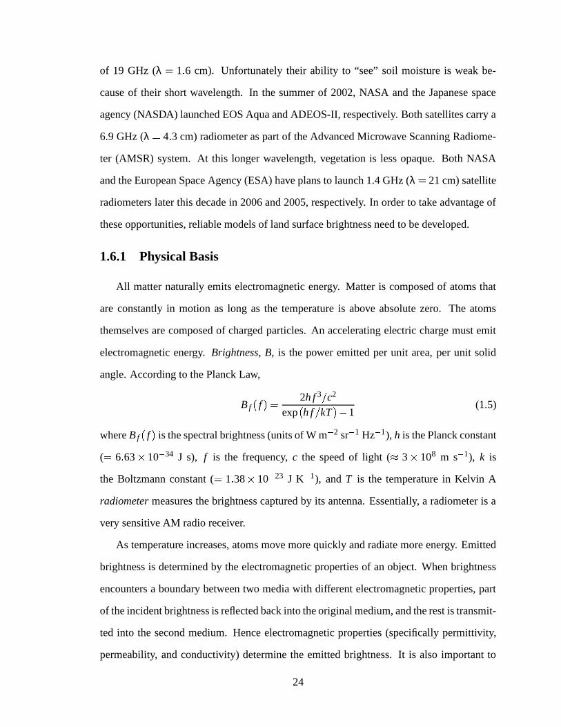
angle. According to the Planck Law,

B ff

2h f 3 c2

exph f kT 1

(1.5)

where B ff is the spectral brightness (units of W m

2 sr 1 Hz

1), h is the Planck constant

( 6 63 10 34 J s), f is the frequency, c the speed of light ( 3 108 m s

1), k is

the Boltzmann constant ( 1 38 10 23 J K

1), and T is the temperature in Kelvin A

radiometer measures the brightness captured by its antenna. Essentially, a radiometer is a

very sensitive AM radio receiver.

As temperature increases, atoms move more quickly and radiate more energy. Emitted

brightness is determined by the electromagnetic properties of an object. When brightness

encounters a boundary between two media with different electromagnetic properties, part

of the incident brightness is reflected back into the original medium, and the rest is transmit-

ted into the second medium. Hence electromagnetic properties (specifically permittivity,

permeability, and conductivity) determine the emitted brightness. It is also important to

24

note that these properties are frequency dependent.

Take for example a radiometer measuring the brightness of moist soil. At low frequen-

cies, moist soil and air have very different electrical properties because of water’s high

permittivity. Hence the power emitted from a moist soil halfspace is much less than the

power emitted from a dry soil halfspace whose electrical properties are more similar to air.

In the first case, more of the brightness is reflected back into the soil and less is transmitted.

As the water content decreases, the electromagnetic contrast between the soil and the air

decreases and the soil appears brighter. At higher frequencies, water no longer has a high

permittivity and hence the brightness of wet and dry soil are very similar. If two objects

are at the same temperature, the object with a higher emissivity is brighter. A blackbody

is a perfect emitter (no reflection occurs at the surface boundary) and has an emissivity of

unity. A highly polished metal surface can have an emissivity close to zero.

1.6.2 Brightness Temperature

If h f kT 1, then exph f kT 1 h f kT and (1.5) simplifies to

B 2kλ2 T (1.6)

where λ is the free–space wavelength and a small but finite range of frequencies sampled

has been assumed. This is called the Rayleigh–Jeans Law and it is valid for low frequen-

cies ( 100 GHz, most of the microwave region) and naturally–occurring temperatures in

Earth’s environment.

Since Planck Law radiation is completely unpolarized, half of the brightness is horizontally–

polarized and half is vertically–polarized. Hence

Bp

12

B k

λ2 T (1.7)

where Bp is the p–polarized brightness. Because the magnitude of brightness is so small

and nonsensical ( 10 18 W m

2 sr 1 at microwave wavelengths), the p–polarized bright-

ness is normally represented by a brightness temperature, TB. The brightness temperature

25

corresponds to the thermometric temperature of a blackbody radiator that would produce

the same p–polarized brightness:

Bp

kλ2 TB (1.8)

where the subscript p has been deleted on the brightness temperature because polarization

dependence is assumed. The brightness temperature has units of Kelvin and gives a better

sense of whether objects are “cold” (have a low temperature and/or low emissivity) or “hot”

(high temperature and/or high emissivity). For an object with a uniform temperature, its

emissivity is then the ratio of its brightness temperature to its thermometric temperature:

e TB T (1.9)

For objects in thermal equilibrium with their surroundings,

e 1 R (1.10)

where R is the reflectivity of the interface.

1.6.3 Why Microwaves?

The emissivities of most natural surfaces do not vary greatly at infrared wavelengths.

On the other hand, microwave emissivity is strongly dependent upon the composition and

structure of the surface or volume under observation. Specifically, microwave emissivities

vary strongly with surface roughness, internal structure, polarization, look–angle [England

and Johnson, 1977], and particularly water content due to liquid water’s high permittivity

at microwave frequencies. It is precisely liquid water’s distinct electromagnetic properties

that make microwave remote sensing sensitive to the water content of soil and vegetation.

Because of their longer wavelength, microwaves penetrate vegetation and soil in contrast

to high–frequency optical and infrared radiation. As a result, modest vegetation is semi–

transparent and the soil beneath the canopy is “visible” to a microwave radiometer. Mi-

crowaves, unlike optical and infrared radiation, also have the ability to penetrate clouds

(including ice clouds) and, to some extent, rain [Ulaby et al., 1981-1986].

26

Courtesy T. Jackson, USDA ARS Hydrology and Remote Sensing Lab

150 K 300 K 5% 50%

Brightness Temperature Soil Moisture

0 10 20 30 40 50 60 70 80 900

50

100

150

200

250

300

antenna incidence angle, °

brig

htne

ss te

mpe

ratu

re a

t 1.4

GH

z, K

10% volumetric soil moisture40% volumetric soil moistureH−polarizationV−polarization

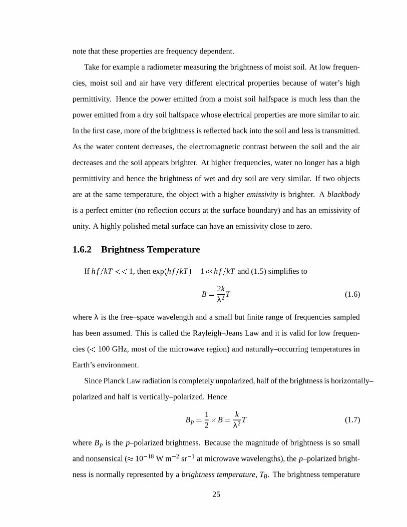
Figure 1.10: At left, the horizontally– and vertically–polarized brightness temperature of asmooth bare soil surface as a function of incidence angle for wet and dry soil. At right, anexample of a soil moisture map derived from a map of brightness temperature.

The graph at left in Figure 1.10 illustrates the effects of polarization, look–angle, and

moisture content on the microwave brightness of a smooth bare soil surface. Note the

Brewster angle at vertical polarization, the angle at which R 0 and e 1. Horizon-

tal polarization is preferred since the difference in brightness between wet and dry soil is

maintained out to large incidence angles. This difference in brightness ( 100 K) is large

in relation to the precision of typical microwave radiometer ( 1 K) and results in an ex-

cellent signal–to–noise ratio. Theoretically, changes in soil moisture of less than 1% can

be measured. At right in Figure 1.10 is an example of a soil moisture map made using an

airplane microwave radiometer. Note how cold brightness temperatures correspond to wet

areas.

The depth to which radiometry is sensitive to soil moisture scales with wavelength. At

1.4 GHz (λ 21 cm), there is sensitivity to the first 4 to 5 cm, while at 19 GHz (λ

1 6 cm), there is sensitivity only to the first few millimeters. This “emitting depth” can

change depending on how sharply the soil constitutive properties vary with depth. Instead,

27

15 20 25 30 35150

175

200

225

250

275

300

21 cm (1.4 GHz)

S = −2 K %−1

4.3 cm (6.9 GHz)

S = −0.9 K %−1

1.6 cm (19 GHz)

S = −0.03 K %−1

brig

htne

ss te

mpe

ratu

re, K

soil moisture, %

M = 1 kg m−2

15 20 25 30 35150

175

200

225

250

275

300

1.6 and 4.3 cm

21 cm

S = −1 K %−1

brig

htne

ss te

mpe

ratu

re, K

soil moisture, %

M = 4 kg m−2

Figure 1.11: Modeled brightness temperature as a function of volumetric soil moisture atthree different wavelengths, for vegetation column densities of M 1 and 4 kg m

2 foran ideal, nonscattering canopy. The soil is treated as a uniform halfspace, and soil andvegetation temperature is 295 K. S is the sensitivity of brightness to soil moisture.

it is more useful to speak of the impedance match between the soil and the air, i.e. how

reflective the soil surface is. At 1.4 GHz, this reflectivity is sometimes determined by only

the first centimeter when the soil moisture profile is sharp (very wet just at the surface)

[Jackson et al., 1998]. On the other hand, when the soil is very dry and the moisture

profile is uniform, the reflectivity can depend on the first several centimeters [Schmugge

and Choudhury, 1981].

28

1.6.4 Effect of Vegetation

At microwave frequencies, the brightness of a vegetated surface is determined by both

the state of the canopy and the underlying soil. The vegetation type, stage of growth, den-

sity, temperature, and moisture content, as well as the soil water content, soil type, rough-

ness, and temperature are all important factors. When the canopy has a sufficiently low

column density, microwave brightness is most sensitive to soil water content [Schmugge,

1978; Newton and Rouse, 1980; Wang et al., 1980b; Jackson et al., 1982; Ulaby et al.,

1983]. At higher column densities, vegetation gradually becomes opaque until no sensitiv-

ity to soil moisture can be seen.

The two graphs in Figure 1.11 illustrate the effect of vegetation column density on

the relationship between brightness temperature and soil water content at three different

microwave wavelengths. Vegetation column density, M, is the integrated vertical mass

of vegetation matter per unit horizontal area. For a column density of M 1 kg m 2

equivalent to a 30 cm high corn crop, there is little sensitivity at λ 1 6 cm, while at

λ 4 3 and 21 cm there is approximately a 1 and 2 K change per volume percent soil

moisture, respectively. At a column density of M 4 kg m 2 equivalent to a 1.5 m corn

crop, only radiation at λ 21 cm (1.4 GHz) shows any change with soil moisture.

As the wavelength increases, microwave brightness originating from the soil suffers

less attenuation by vegetation. At short wavelengths, the canopy effectively becomes in-

finitely thick even at modest levels of column density. At 1.4 GHz, the vegetation column

density at which there is no longer practical sensitivity to soil moisture appears to be about

8 kg m 2 (equivalent to a dense, mature corn canopy) [Wang et al., 1984], while at a higher

frequency such as 6.9 GHz, the limit is at most half as much. Longer wavelengths are also

preferred because they are less susceptible to soil surface roughness and soil and canopy

heterogeneity. The challenge at long wavelengths is to construct satellite instruments that

effectively balance size and weight restrictions with footprint size (spatial resolution). New

technology mentioned previously promises to make these types of satellites possible.

29

−2.5 −2 −1.5 −1 −0.5 0 0.5 1

radiometric sensitivity, K K−1 or K %−1

soil moisture

soil temperature

vegetation moisture

vegetation temperatureM = 1 kg m−2

M = 4 kg m−2

Figure 1.12: Radiometric sensitivity to vegetation temperature, soil temperature, soil mois-ture, and vegetation moisture for an ideal, nonscattering canopy at 1.4 GHz.

Anticipating forthcoming satellite radiometers at 1.4 GHz, much work has been done

at this frequency with ground–based and airplane instruments within the last two decades.

Although the response to changes in soil water content has been well documented, there are

still many questions about the effect of the overlying vegetation. Besides column density,

are there other canopy properties that can significantly affect the microwave brightness?

Figure 1.12 displays the 1.4 GHz radiometric sensitivity to soil moisture along with sensi-

tivity to soil temperature, vegetation temperature, and vegetation moisture as predicted by

a zero–order radiative transfer model. Note that brightness decreases as soil moisture in-

creases, while the other changes tend to increase the brightness. At low vegetation column

densities, sensitivity to soil moisture dominates. For M 1 kg m 2, soil moisture sensi-

tivity is 2 K per volume percent, as illustrated in Figure 1.11. As the column density

increases, the radiometric sensitivity to soil temperature and vegetation temperature and

moisture become comparable to soil moisture sensitivity.

In the past, changes within the canopy, both in temperature and moisture content, have

been assumed to be small. Can these changes be neglected? At higher column densities

30

−8 −6 −4 −2 0 2 4anticipated change in brightness temperature, K

soil moisture (4%)

vegetation moisture (?) ?

vegetation temperature (10 K)M = 1 kg m−2

M = 4 kg m−2

Figure 1.13: Anticipated change in 1.4 GHz brightness temperature in response to changesin vegetation temperature (10 K variation in diurnal cycle) and soil moisture (desire sensi-tivity to 4%) in a nonscattering canopy. Expected change in vegetation moisture not known.

when the soil moisture sensitivity is small but still measurable, these other factors will

have competing influences. Figure 1.13 shows the expected change in 1.4 GHz brightness

temperature given expected changes in vegetation temperature (assuming a typical diurnal

variation of 10 K) and desired soil moisture sensitivity (to 4% by volume). At M

4 kg m 2, these changes are almost equal in magnitude.

What is not immediately known is what changes in vegetation water content can be ex-

pected and thus the corresponding change in brightness. Furthermore, are the predictions

of the zero–order radiative transfer model, suitable for a nonscattering canopy, represen-

tative of what may happen in a canopy such as corn where scattering may be significant?

These are some of several questions this dissertation seeks to answer:

Can scattering of radiation within a corn canopy be neglected at 1.4 GHz? The most

widely used model for land surface microwave brightness (the zero–order radiative

transfer model) assumes negligible scattering, but it has only been validated at steep

angles of incidence at which the vegetation has the least impact.

At what level of vegetation column density is there no longer any useful sensitivity to

changes in soil water content in a corn canopy? Does the transparency of a general

31

canopy depend on simply the amount of vegetation or water in the canopy or also on

its distribution?

What effect do changes in vegetation water content have upon the emitted microwave

radiation? These variations can be caused by intercepted precipitation and dew, or

by slower, more subtle processes such as diurnal variations, senescence, and plant re-

sponse to drought or extreme wetness. Are these changes the same in both scattering

and nonscattering canopies?

1.7 Format of Dissertation

The second chapter of this dissertation describes experiments during which radiometric

and micro–meteorological data were collected in a field of corn, and the instruments used

to collect these data. The third chapter discusses the electromagnetic properties of a corn

canopy in terms of the nature of absorption, emission, and scattering. It also determines

whether the zero–order radiative transfer model is suitable for scattering canopies such as

field corn. A new zero–order model is formulated. The fourth chapter compares the new

model with observations. It then examines the effect of changes in canopy water content on

the microwave brightness of field corn, due to intercepted precipitation and dew. Finally,

the sensitivity to soil moisture in field corn observed in this and other investigations is pre-

sented. The competing effects of vegetation temperature and moisture and soil moisture

are also detailed for both a scattering canopy such as field corn and a hypothetical nonscat-

tering canopy such as thick grass. Finally, the fifth chapter discusses the contributions of

this thesis to the general body of research, and future work in this subject area.

32

CHAPTER 2

The Eighth Radiobrightness and Energy BalanceExperiment

The Eighth Radiobrightness and Energy Balance EXperiment (REBEX–8) was con-

ducted by members of the Microwave Geophysics Group at the University of Michigan

during 2001. The goal of the experiment was to record simultaneous, long time–series

measurements of microwave brightness, soil moisture, and relevant micrometeorology on

the plot scale, at several different stages of growth and under various environmental condi-

tions in a “complex” vegetation canopy. A complex canopy is loosely defined as one that

contains significant small–scale heterogeneity in the form of different canopy components,

such that scattering may be important at microwave wavelengths. The particular canopy

observed in REBEX–8 was a field corn canopy. The plot scale is defined as an area on the

order of 102 m2, which lies between a scale encompassing the entire field (order 106 m2)

and fine–scale field variations such as tilled row structure (order 100 m2). Radiometer

footprints varied from approximately 20 to 40 m2, depending on the incidence angle, and

encompassed several rows.

This approach to studying land surface microwave brightness is seldom used. Tradi-

tional remote sensing studies attempt to replicate satellite measurements, in which discrete

measurements of brightness are made only once every one to three days. Continuous mea-

surements of brightness, micrometeorology, and soil state allow the integration of many

types of observations with models of land–atmosphere interaction and microwave bright-

33

Figure 2.1: Truck–mounted radiometers and micrometeorological station on day of year144, looking southeast.

ness. Together, they can be used to tease out many subtle, yet important physical properties

that might otherwise be hard to find, much like using the context of a sentence to decipher

an unknown word as opposed to only examining the word itself.

The experimental site, an 800 (E–W) by 400 m (N–S) privately–owned corn field under

conventional tillage and crop rotation, was located in Southeastern Michigan approximately

40 km south and west of North Campus of the University of Michigan. The site was

unusually flat and uniform in terms of soil properties and vegetation. See Figure 2.1 for a

picture of the site and equipment in late May. The soil at the site was a silty clay loam of

the Lenawee series. Soil texture was measured by the Kansas State University Agronomy

Department’s Soil Testing Laboratory and found to be 16.1% sand, 55.0% silt, 28.9% clay

for the first 10 cm soil layer, with slightly less than 2% total carbon. Average row spacing

was 0.77 m. Plant density was 7.49 m 2. Rows were planted E–W.

Five distinct experiments of one to four days each were conducted at different times

during the spring, summer, and fall to observe different stages of vegetation growth. Ta-

34

ble 2.1 describes the vegetation conditions during each REBEX and a labeling convention.

The field was planted on April 29 and 30 (day of year 119 and 120) and harvested on

October 17 and 18 (day of year 290 and 291). Between REBEX–8 and REBEX–8x1, all

equipment was removed from the field to accommodate cultivation on June 11 and 12 (days

of year 162 and 163). After June 25 (day of year 176) the fraction of vegetation cover was

unity. The experiments after cultivation are collectively referred to as REBEX–8x. Mea-

surements of microwave brightness were only measured during each experimental period.

Micrometeorology was measured continuously from the middle of May through the middle

of October, save for the cultivation period.

Leaf–area index (LAI) and vegetation and water column densities were measured pe-

riodically throughout the summer. Each LAI value was computed from the average of ten

samples taken at random locations separated by 5 to 10 m within the field. Each sample

made use of one above–canopy measurement and the average of three below–canopy mea-

surements of the incident radiation. Below–canopy measurements were made in the row,

and one–third and two–thirds of the way across the row space. The wet and dry masses of

six randomly chosen plants were averaged to compute column densities. Each plant was

separated by component (stem, leaves, and ear). Samples were placed in paper bags and

dried in a 70

C oven for 7 days.

REBEX–7, a supporting field experiment, was conducted the previous summer in a

field of corn 1 km north of the REBEX–8 site. This field had nearly identical topography

Table 2.1: REBEX information. Date information includes days of year. GS refers tovegetation growth stage. H is vegetation height in meters. M is vegetation column densityin kg m

2. Mw is water column density in kg m 2. LAI is leaf area index in m2 m

2.Dates GS H M Mw LAI

REBEX–8 May 23-25 (143-145) effectively bare soil 0.2 0.3 0.3 0.1REBEX–8x1 July 4 (185) growing 1.8 4.8 4.3 3.2REBEX–8x2 July 11-13 (192-194) growing 2.2 5.7 5.0 4.0REBEX–8x3 Aug 17-20 (229-232) mature 3.0 8.0 6.3 4.8REBEX–8x4 Oct 10 (283) senescent 2.8 4.9 2.7 2.5

35

Laberdee Rd

Holloway Rd

Hoa

glan

d H

wy

Pio

tter

Hw

y

Section 27Ridgeway TwpLenawee Cty

Michigan

W Half of SE Quarterand

E Half of SW QuarterSection 27

Laberdee Rd

Pio

tter

Hw

ywoods

rows running E and W

N

MMS towerlane

15 feet wide~0.2 mile long

~0.47 mile

~0.4

7mil

e

TMRS

Schwab Drain

Swam

p Ra

isin

Cree

k

beans

0 200

0 0.1 0.2 0.3 0.4 0.5 mile

400 600 m

Figure 2.2: Map of REBEX–8 and –8x site. Truck–mounted radiometers (TMRS) andMicro–meteorological station (MMS) marked.

and soil and vegetation properties. The same implements and procedures were used to

plant and cultivate the corn. Many of the same measurements made in REBEX–8 were

also made the previous summer in REBEX–7.

2.1 Microwave Radiometers

Two 1.4 GHz radiometers, oriented to record horizontally–polarized (H–pol) and vertically–

polarized (V–pol) brightness, were mounted on the hydraulic arm of a truck. The arm, along

with a rotator at the end of the arm, made it possible to change both the incidence angle, θ,

and the azimuthal angle, φ, at which the radiometers received radiation. Azimuthal angle

was measured with respect to row direction, with φ 0

parallel to the row direction. An-

tennae E– and H–plane half–power beamwidths were approximately 21

. Side lobe levels

were below -20 dB. Terrain brightness was measured at two–minute intervals. The truck

36

was positioned within the field at the head of a “lane”, a portion of the field that was not

planted. The lane, 6 rows wide and approximately 250 m long, began at the eastern edge of

the field and continued west. The antenna footprints were located at the head of the lane,

to the west (φ 0

) and to the south (φ 90

). See Figure 2.2 for a map of the site.

Due to the radiometer fabrication schedule, only one radiometer was available during

REBEX–8. It was oriented to measure H–pol 1.4 GHz brightness. Both radiometers were

deployed for all subsequent field experiments. Unknown equipment problems with the H–

pol radiometer contaminated many data and only H–pol brightness measurements during

REBEX–8x3 and –8x4 were usable. Measurements of V–pol 1.4 GHz brightness were

successfully made during REBEX–8x1, –8x2, –8x3, and –8x4.

2.1.1 Direct–Sampling Digital Radiometer (DSDR)

The input signal to a radiometer is the time–varying antenna voltage associated with

the intercepted power. This voltage signal is essentially random noise and can be described

by a zero–mean Gaussian (normal) probability distribution. In particular, the amplitude

of the voltage is normally distributed, while the envelope is Rayleigh distributed. Since

power is directly proportional to the square of the voltage, the expected value of the power

(or power estimate) is proportional to the expected value of the square of the voltage, also

known as the voltage’s variance. The corresponding power has an exponential distribution.

The average power is equal to the standard deviation of a single measurements of power.

A traditional radiometer (one with a superheterodyne receiver) uses a mixer to down–

convert the high frequency input signal. A Direct–Sampling Digital Radiometer (DSDR)

[Fischman, 2001], on the other hand, employs a fast A/D converter to sub–harmonically

sample (and effectively down–convert) the input voltage signal. Subsequent digital hard-

ware then operates on the signal (which is now just a stream of numbers) to measure the

input power. The output of a DSDR is a single number that is the average of N samples of

the square of the quantized voltage signal, Q v tn 2, sampled at time tn. It is called the rQ

37

value:

rQ

1N

N

∑n 1

Q v tn 2 (2.1)

The rQ value is simply a time–limited estimate of the variance of the quantized voltage,

which is an estimate of the power captured by the radiometer’s antenna as discussed earlier.

The A/D converter must have a minimum number of quantization levels within the

input signal voltage range in order to measure its power. This is determined using a param-

eter called the normalized signal strength, s, defined as the standard deviation of the input

signal, σ, normalized by the discretization step size (quantization voltage), vo, of the A/D

converter:

s σ vo (2.2)

The radiometers deployed in REBEX–8 and –8x used SPT7610 flash A/D converters man-

ufactured by Signal Processing Technologies (Colorado Springs, Colorado). Their small–

signal bandwidth was 1.4 GHz and their discretization step size was vo 1 V 26 bits

15 625 mV bit 1. Small–signal bandwidth is defined by the manufacturer as the fre-

quency at which the sampler and digitizer attenuate the input signal by 3 dB when the input

signal is 20 dB below the full-scale input range of the A/D converter. Since the full–scale

input range is 1 V, the small-signal input signal would be 100 mV. When attenuated by

3 dB, the resulting signal is approximately 71 mV. Dividing by the discretization step size

gives the effective number of digitization levels within the small–signal bandwidth around

1.4 GHz:

71 mV 15 625 mV 4 5 levels (2.3)

Since the effective range of a Gaussian signal is 6σ, the 4.5 levels must span 6s and

therefore:

6s 4 5 s 4 5 6 0 75 (2.4)

Hence these A/D converters satisfy the large signal approximation of s 2 3 as defined

by Fischman [2001]. When this condition is satisfied, the difference between an rQ value

38

obtained with a ideal A/D converter of infinite resolution and the rQ value from a real

A/D converter has reached a constant value of vo2 12. In reality, rQ

vo2 is what is actually

recorded in a DSDR output data file. To correct for the noise introduced by the quantization

process, 1 12, was subtracted from a DSDR output.

2.1.2 DSDR Precision

Accuracy is a measure of how close a measurement is to the real value. Precision is

the closeness of agreement among several measurements of the same quantity. Precision

can also be thought of as the reproducibility of a measurement or the sensitivity of the

instrument in terms of the minimum detectable change. The accuracy of a radiometer’s

measurement of terrain brightness temperature depends on the calibration procedure and

the radiometer’s stability. Calibration accuracy is difficult to quantify and is discussed later.

A radiometer’s precision is commonly called its noise–equivalent sensitivity, or NE∆T .

There are three main sources of noise which degrade the NE∆T of a DSDR:

1. Random DC bias fluctuations in the A/D converter, ∆TL;

2. The finite number of samples, ∆TF ;

3. Gain change due to random temperature fluctuations, ∆TG.

Because these effects are independent,

NE∆T

∆TL2 ∆TF

2 ∆TG2 (2.5)

Previously it was shown that the quantization process introduces a bias, but it can be

removed easily. The A/D converter also introduces noise associated with random DC bias

fluctuations. Fischman [2001] formulated an uncertainty function of a DSDR’s digital

correlator, fLs , which describes the noise associated with DC bias fluctuations:

∆TL Tsys

fLs

2 3s2(2.6)

39

where Tsys is the noise temperature of the antenna and analog hardware before the A/D

converter. For s 0 75, fLs is approximately 6 10

5 (Figure 2.4 of Fischman [2001]).

For a typical radiometer with Tsys of 400 K, ∆TL 0 01 K.

Earlier the rQ value was described as a time-limited estimate of the expected value. The

actual expected value of a signal can only be found after an infinite number of samples have

been recorded. The sensitivity contribution due to a finite sampling time is

∆TF

Tsys

N(2.7)

where N is the number of independent samples of the incident brightness that are averaged

together to determine the final measurement. N fs τ, where the digital sample rate fs

1 tn. In REBEX–8 and –8x, fs 5 MHz and τ 1 s, which yields N 5 220 5

106 samples. Accordingly, ∆TF 0 2 K for a typical Tsys of 400 K.

Finally, the gain, G, of the amplifiers used to boost the antenna voltage to a measurable

level is sensitive to changes in temperature:

∆TG Tsys

∆GG

(2.8)

For the amplifiers used in REBEX–8 and –8x,G ∆G G 0 06 dB for every 1

C

change in the physical temperature of the amplifier. Hence,

∆GG

Tsys

G ∆G

G 1 Tsys

5 5 K

C 1 (2.9)

for a typical Tsys of 400 K. Given an amplifier temperature fluctuation σamp 0 09

C,

as measured during REBEX–8x4 (Figure 2.3), ∆TG 0 5 K. The total DSDR sensitivity,

according to (2.5) is then:

NE∆T 0 012 0 22 0 52 0 5 K (2.10)

Figure 2.4 displays measured NE∆T during REBEX–8x4. V–pol NE∆T is slightly

lower than 0.5 K. This may be because during this short observation interval, temperature

fluctuations may have been lower than for the entire period (as illustrated by Figure 2.3

40

229 229.5 230 230.5 231 231.5 23219.8

19.9

20

20.1

20.2

20.3

20.4

20.5

20.6

20.7

20.8temperature data for REBEX−8x3 v−pol

day of year, 2001

tem

pera

ture

, °C

amplifier temperature, σamp

= 0.07 °C

reference load temperature, mean = 20.16 °C

Figure 2.3: Amplifier and reference load temperatures for the V–pol DSDR duringREBEX–8x3.

during REBEX–8x3). Actual V–pol DSDR Tsys may also have been lower than the rough

estimate of 400 K, and may have changed over time. At H–pol, NE∆T was considerably

higher because of the poor temperature control experienced by the H–pol DSDR during

REBEX–8x4 (σamp 0 3

C). Table 2.2 lists σamp for all REBEXs. Note that save for

REBEX–8x4, σamp for both DSDRs was always 0 1 K and NE∆T was at most 0.5 K.

Table 2.2: Amplifier temperature variation, σamp, and approximate NE∆T during REBEX–8 and –8x assuming Tsys

400 K.R8 (H) R8x1 (V) R8x2 (V) R8x3 (H, V) R8x4 (H, V)

σamp

C 0.06 0.08 0.07 0.08, 0.07 0.30, 0.09NE∆T , K 0.4 0.5 0.4 0.5, 0.4 1.7, 0.5

41

277

279

281

283

tem

p, K

1.5 cm soil

veg IR

255

257

259

261

brig

htne

ss te

mp,

K

V−pol, NE∆T = 0.3 K

7:40 7:44 7:48 7:52 7:56 8:00

229

231

233

235

brig

htne

ss te

mp,

K

LDT on day of year 283

H−pol, NE∆T = 1.7 K

Figure 2.4: An example of radiometer precision during REBEX–8x4. Soil and vegetationtemperatures and soil moisture (not shown) were essentially constant during the 20–minuteperiod between 7:40 and 8:00 Local Daylight Time (LDT). Presented NE∆T is for the 10brightness temperature measurements made during this period.

2.1.3 DSDR Calibration

Typically, microwave radiometers are calibrated by filling the beam of the antenna with

objects of known brightness temperature. If the relationship between the radiometer output

(a voltage in the case of a traditional radiometer, the rQ value for a DSDR) and brightness

is linear, only two calibration points are needed. Such is the case for both DSDRs used in

REBEX–8 and –8x. To make an accurate calibration, the actual brightness of the calibration

targets must be measured or found in some other way. It is also desirable to have contrasting

brightnesses, very “cold” and very “hot” brightness temperatures.

The sky is a perfect calibration load at 1.4 GHz because it is very cold (about 8 K),

beamfilling, and very stable. At the top of the atmosphere, the brightness temperature of

the sky has two components: Tcos, the cosmic background (2.7 K); and Tgal , the direction–

42

Figure 2.5: At left: absorber calibration. At right: microwave absorber.

dependent brightness from our own galaxy. Tgal was calculated using radioastronomy sky

maps at 1.4 GHz and taking into account the position of Earth relative to the galactic center.

At the earth’s surface, a up–looking radiometer will also measure downwelling atmospheric

emission, Tatm, as well as the extra–terrestrial radiation attenuated by the atmosphere:

Tsky Tatm

Tcos Tgal L (2.11)

where L is the atmospheric attenuation. Both Tatm and L were calculated with radiosonde

measurements of temperature and humidity made twice daily at the National Weather Ser-

vice office in White Lake, Michigan, about 90 km north and east of the site. At 1.4 GHz,

the atmospheric attenuation and emission are small (in the absence of hydrometeors) and

does not vary much from day to day.

Usually a microwave absorber is used as the “hot” source. If the absorber is nearly

a blackbody, its brightness temperature can be approximated by its physical temperature.

Figure 2.5 illustrates the absorber calibration procedure and the piece of absorber used.

Absorber calibration was not successful. Two possible reasons were determined. First, the

absorber used may not have been appropriate at 1.4 GHz. The pyramids of the absorber

may have been too small (much less than a wavelength), its emissivity less than unity, and

hence the brightness temperature may have been considerably different from its physical

43

temperature. The absorber also may have had some degree of transparency at 1.4 GHz. Al-

though the absorber was backed with aluminum foil, the backing was not uniform. Second,

the absorber may not have been beamfilling. In an attempt to fill the beam, the absorber

was held very close to the antenna aperture, well within the near–field of the antenna where

the antenna pattern is not known. Because it was manually positioned, the location of the

absorber, both in terms of its coverage of the aperture and its distance from the antenna rim,

changed during each calibration attempt. In contrast to when the antennae were pointed at

the sky, consecutive rQ measurements of the absorber varied considerably.

In its place, the internal reference loads were used to calibrate the DSDRs. Although

reference load physical temperature was well known, small electrical losses associated with

the antenna and the coaxial cable connecting the antenna to the radiometer result in some

error so that if the brightness of both the reference load and the scene viewed by the antenna

were actually the same, they would be recorded as two different brightnesses. Given these

circumstances, the accuracy of both DSDRs were estimated to be within

2 K.

The internal reference load was also used to adjust the calibration for changes in system

gain observed during the experiments. Two types of gain change were observed: a slow

change likely due to diurnal temperature fluctuations of the radiometer components; and

sharp changes resulting from changes in radiometer orientation. Although the temperature

of the electronics close to the amplifier was stable, the other parts of the radiometer ex-

perienced changes in temperature. As coaxial cables and connectors warm and cool, their

electrical properties change slightly. Most of the evidence collected point to an A/D con-

verter temperature dependence. Sharp changes in gain were observed when the incidence

angle of the radiometer was adjusted. Possible explanations include redistribution of heat

within the radiometer and mechanical stress on the radiometer electronics. As is demon-

strated in later chapters by the quality of the resulting brightness temperature observations,

the gain–change compensation procedure described below worked well.

Figure 2.6 illustrates the compensation procedure. Brightness temperature measure-

44

TB_sky

Tref

rQ_ant,sky rQ_ref,sky

pivot point

TB

rQ

cal line from sky measurement

subsequent rQ_ref at time trQ_ant at time t

TB at time t

cal line at time t

Figure 2.6: DSDR calibration procedure.

ments of both the antenna and internal reference load were made during every measure-

ment cycle. The initial calibration line was established during the sky measurement. Two

pairs of rQ and brightness temperature, from the sky (rQ ant sky and TB sky) and from the

reference load (rQ re f sky and Tre f ), specified the slope and y–intercept of the line. At a

later time t, rQ re f would change despite the fact that Tre f had not, signaling a change in

system gain. The new rQ re f and Tre f (which was assumed to be constant) were used to find

the slope of a new calibration line, the dashed line in Figure 2.6. The y–intercept (marked

“pivot point”) was not allowed to change. It represents the amount of “negative brightness”

that would have to be captured by the antenna to completely cancel the self emission, or

noise of the radiometer. This noise, denoted Trec in the microwave remote sensing litera-

ture, actually does change with temperature but the effect on the output is small relative

to temperature–induced gain changes. Here the change in Trec was assumed to be zero.

At rQ 0, gain change is of no consequence and this hypothetical negative brightness is

constant. The x–intercept (the rQ value when TB 0 K) represents the self–emission of the

radiometer since this is the power measured when no power is intercepted by the antenna,

i.e. the scene brightness temperature is 0 K. This self emission does change with system

gain, and hence the x–intercept changes over time.

45

228.5 229 229.5 230 230.5 231 231.5 232 232.51.85

1.875

1.9

1.925

1.95

1.975

2

2.025

2.05

day of year, 2001

refe

renc

e lo

ad r Q

, dim

ensi

onle

ss

REBEX−8x3 H−pol

original datapolynomial fit

Figure 2.7: Recorded reference load rQ and fitted polynomial for the H–pol DSDR duringREBEX–8x3.

As stated above, the temperature of the reference load was assumed to be constant.

From Figure 2.3, it can be seen that this is a good assumption over long periods of time, but

there is considerable variation from measurement to measurement. This variation is close

to the σamp described above, but not exactly because the amplifiers and reference load were

not subjected to exactly the same thermal environment as evidenced by the slight, but con-

sistent, temperature difference. If not taken into account, this thermal noise would degrade

NE∆T . To compensate for these short temperature fluctuations of the reference load, a

polynomial fit of rQ re f , instead of the actual rQ re f measurements, was used to adjust the

slope of the calibration line. Figure 2.7 shows actual rQ re f measurements and the polyno-

mial fit for the H–pol DSDR during REBEX–8x3. Note the rapid changes in short–term

46

Figure 2.8: Laser profiler.

temperature on top of a smooth, slow variation, obviously the result of a diurnal tempera-

ture change. This was typical of the H–pol DSDR. The V–pol DSDR, on the other hand,

was more susceptible to sharp changes in gain associated with rotation of the radiometer.

The same polynomial fitting procedure was used to smooth the V–pol rQ re f variations.

This compensation procedure is valid because the reference load was not subject to direct

thermal control as were the amplifiers. The time constant of the reference load temperature

change is much greater than the integration period.

2.2 Laser Profiler

A laser profiler was used to measure soil surface height variations during REBEX–

7. It is pictured in Figure 2.8. The profiler had a horizontal resolution of 1 mm and a

vertical precision on the order of 10 2 mm. Four one–meter transects perpendicular to row

direction of undisturbed soil in the REBEX–7 field were measured on August 25, 2000,

(day of year 238) under conditions very similar to what was present during REBEX–8x3.

These four transects were oriented end–to–end and covered seven rows.

Two examples of the surface height profile are shown in Figure 2.9. The depression

47

100 200 300 400 500 600 700 800 900 100090

100

110

120

130

140

150

160

170

heig

ht, m

m

distance, mm

August 25, 2000, @ 12:32 LDT

100 200 300 400 500 600 700 800 900 100070

80

90

100

110

120

130

140

150

distance, mm

heig

ht, m

m

August 25, 2000, @ 14:15 LDT

Figure 2.9: Two examples of recorded soil surface profile.

at 500 mm in the top profile is the row, the point at which a stem of a corn plant would

be. Recall that the average row spacing was 0.77 m. Note the generally “high” area from

approximately 400 to 850 mm. The bump between 200 and 300 mm may have been a clod

or vegetation debris. In the bottom figure, the row depression is just before 700 mm, and

the 0 to 700 mm region represents almost an entire row space. The depression at 400 mm

was likely a crack in the soil.

There are two quantities often used to characterize a rough surface. The first is the

standard deviation of the surface height (or rms roughness), σs. The second is the correla-

tion length, lc, which describes the similarity in height of two points separated by a certain

distance, or lag. A surface with a high level of large–scale roughness would have a short

lc, meaning that the surface height changes quickly as you move away from a given point.

48

0 100 200 300 400 500 600 700 800 900 1000

−0.6

−0.4

−0.2

0

0.2

0.4

0.6

0.8

1

lag, mm

corr

elat

ion,

dim

ensi

onle

ss

Figure 2.10: Computed correlation function.

One example would be freshly tilled soil, where the height variation changes quickly due

to large, broken clods. An example of a surface with a long correlation length is a large

body of water. The ratio σ lc is a measure of the average slope of a surface.

Calculation of σs, is straight–forward. The correlation function, ρ, is computed:

ρn

1N n 1 ∑N n

j 1 zj z

j n

1N 1 ∑N

j 1 zj 2

(2.12)

where n is the lag, N is the total number of points measured, and zj is the height of the

jth point along the transect. The correlation length is defined as ρlc 1 e 0 3679. The

numerator of (2.12) is the (unbiased) estimate of the height correlation between two points

along the transect separated by a lag of n. This correlation is normalized by the height

correlation of zero lag (which is the surface height variance σs2).

Figure 2.10 is a plot of the average correlation function ρn . For the soil surface in

49

REBEX–7, the average surface height standard deviation was σs 14 mm and the average

correlation length was lc 85 mm. The periodic nature of the row structure is evident: note

that ρ peaks again at precisely the average row width of 0.77 m. In the case of a periodic

surface, the total roughness can be thought of as a random roughness superimposed on a

periodic function. Because the random roughness is uncorrelated to the periodic variation,

the difference between the two peaks in Figure 2.10 represents this random roughness. The

peak of the correlation function at 0.77 m corresponds to a rms height of 0 63 142 11 mm. This is the rms height of the periodic variation. The rms value of the random

roughness is 142 112 9 mm

According to Oh and Kay [1998], surface segments totaling 40σs and 200lc must be

used to accurately characterize these surface parameters. While this condition was satisfied

for σs, lc must be considered a rough estimate. On the other hand, these values match well

those measured by Wigneron et al. [2001] for tilled agricultural fields, particularly their

field 18 with σs 19 mm and lc 66 mm.

2.3 Soil Moisture

The accurate and precise measurements of near–surface soil moisture made on the plot–

scale were one of the highlights of REBEX–8 and –8x. Not only was this the first time

that members of the Microwave Geophysics Group had successfully made continuous soil

moisture measurements, this data set is now one of a very few known data sets of soil

moisture through the emitting depth at 1.4 GHz under a vegetation canopy. A soil–specific

calibration of a hand–held impedance probe was made with gravimetric samples and bulk

density measurements. Approximately one thousand impedance probe measurements were

made over the course of the experiments to calibrate continuous measurements of volu-

metric soil moisture made made by buried time domain reflectometry (TDR) instruments.

The TDR instruments were buried at appropriate depths to match the sample depth of the

impedance probe. When grouped together, the TDR measured 0–3 and 3–6 cm volumetric

50

HL

R8

R8xHL

Figure 2.11: Soil topography during REBEX–8 and REBEX–8x reduced to a binary repre-sentation.

soil moisture. In the following sections, the methods and materials used to make these

measurements are presented along with error analyses.

2.3.1 Measurement Technique

Planting and cultivation produce distinct localized soil topography in agricultural fields

[Kaspar et al., 1995]. This topography was reduced to a binary representation of high

(H) and low (L) areas as a practical way to retain this unique row structure. Figure 2.11

illustrates the H and L representation. Although only 2 to 4 cm lower than H areas, L areas

were distinct from the rest of the soil surface because of their significantly higher water

content (and resulting darker color), bulk density, and smoother surface. They tended to be

located in the middle of the row space and in the row during REBEX–8, although absent

in every third row space. When the soil was cultivated, the top 5 to 7 cm of the soil in the

middle of the row space was effectively “pushed” towards the rows, creating a L area in

each row space. No distinction was made between trafficked (wheels of tractor or other

machinery) and un–trafficked row spaces. The fractions of H and L areas were determined

by sampling several rows with a metric tape measure. During REBEX–8, 36% of the soil

surface was classified as L. After cultivation, the this fraction changed to 21%.

To find the overall near–surface soil moisture content, TDR instruments were placed at

1.5 and 4.5 cm below the soil surface in both H and L areas. The sample volume of a TDR

instrument has the shape of slightly flattened cylinder of length equivalent to the length of

the transmission lines. The sensing volume extends slightly farther in the plane containing

the two wires of the transmission line than in the perpendicular direction. According to cal-

51

Figure 2.12: TDR during REBEX–8: at left, in a high area at 1.5 cm; at right, in a low areaat 4.5 cm.

Figure 2.13: Impedance probe. Each of the four tines are 6 cm long.

culations performed by Knight [1992], approximately 80% of the sensing volume is within

a 2 cm radius, and slightly more than 90% within a 3 cm radius for the particular TDR

instruments used in REBEX–8 and –8x. When oriented so that the plane containing the

two wires of the transmission line is parallel to the soil surface, Baker and Lascano [1989]

found that TDR instruments have a vertical resolution of approximately 3 cm. Hence the

TDR placed at 1.5 and 4.5 cm measured the 0–3 and 3–6 cm layers, respectively.

Figure 2.12 shows TDR during REBEX–8 placed in an H area at 1.5 cm and in an L

area at 4.5 cm. To install a TDR, a sharp vertical face was cut into the soil and the TDR was

slowly pushed into the face while keeping it level. During TDR installation at the beginning

of REBEX–8 and –8x, the soil was wet and sticky allowing such shallow insertion depths

and reducing the probably of large air gaps that degrade TDR sensitivity [Knight et al.,

1997]. After insertion, soil was replaced under, over, and around the sensor head.

Twelve total TDR instruments were used, evenly divided among H and L areas and

52

Figure 2.14: Orientation of impedance probe and TDR. Top: side view. Bottom: plan view.Drawn to scale.

depths of 1.5 and 4.5 cm. Three individual TDR were averaged together to produce mea-

surements at 1.5 and 4.5 cm in H and L areas. The H and L areas were then weighted

according to their spatial fractions to obtain an overall 0–3 and 3–6 cm measurement. The

TDR were calibrated in-situ with a hand–held impedance probe at several points throughout

the experiments. The impedance probe is pictured in Figure 2.13, and Figure 2.14 illus-

trates the relative orientation of the impedance probe and TDR instruments. When TDR

at 1.5 and 4.5 cm are combined, their vertical sample depth matches the 0–6 cm sampled

by the impedance probe. TDR were not placed directly on top of each other. The diagram

in Figure 2.14 illustrates only the concept of combining 1.5 and 4.5 cm measurements to

obtain a 0–6 cm value.

Impedance probe measurements were made on eight days over the course of the summer

(days of year 143, 144, 145, 185, 187, 194, 229, and 270). On each day, 10 measurements

were made in H areas and 10 measurements were made in L areas at 7 randomly chosen

sites in the experiment area, for a total of 140 measurements (70 H and 70 L) per day.

Each set of ten impedance probe measurements were made at random locations within an

approximately four meter square area. The sites were located on either side of the path

through the field which led from the head of the lane to the micrometeorological station

tower (Figure 2.2). Foot traffic in the field was restricted to this path only. Averaging the H

and L impedance probe measurements calibrated the TDR instruments, buried in adjacent

53

rows to the north and south of the tower, to the field–average near–surface soil moisture.

According to the theory of time–stability [Vachaud et al., 1985], the spatial pattern of soil

moisture persists and hence soil moisture measured at the tower changes in concert with

soil moisture in other parts of the field. Due to the extreme uniformity of the site, the

differences in average soil moisture among sites within the field along the path leading to

the tower were low, always less than 0.04 m3 m 3 and typically less than 0.02 m3 m

3. As

a result, soil moisture within the footprints of the radiometers is assumed to be accurately

measured with TDR buried a considerable distance away near the tower.

2.3.2 Impedance Probe

At frequencies of less than 1 MHz, a variety of factors such as the bulk density, wa-

ter content, water salinity and chemistry, oxidation-reduction reactions, cation exchange

processes, corrosion processes, chemical concentration gradients, clay–organic reactions,

and other phenomena can affect the electrical properties of soil [Olhoeft, 1989]. At higher

frequencies in the MHz and GHz range, water content primarily determines soil electro-

magnetic properties. In non ferro–magnetic soils, it is the soil’s relative permittivity, εr,

which changes with water content. For frequencies below about 20 GHz, the real part of

the relative permittivity of liquid water is about 80 while for the types of minerals typically

found in soil it is around 3 to 5. Moist soil is a combination of water and minerals (as well

as organic matter) and can have a relative permittivity between 3 and 30 in the microwave

region [Hallikainen et al., 1985]. Strong linear relationships between the refractive index,

n εr, and water content for many types of soils have been observed [Topp et al., 1980;

Whalley, 1993; White et al., 1994; Curtis, 2001].

A ThetaProbe ML2x (Delta–T Devices, Cambridge, UK) impedance probe was used to

measure soil water content and subsequently calibrate buried TDR instruments. It consists

of four 6 cm sharpened stainless steel rods that protrude from a 40 mm diameter and 112 cm

long PVC cylinder (Figure 2.13). Three shield rods are spaced equally on a 26.5 mm

54

circle surround the center signal rod. The diameter of each rod is 3 mm. The approximate

volume of soil sampled by the ThetaProbe, a 4 cm diameter, 6 cm long cylinder surrounding

the signal rod, is approximately 75 cm3. This impedance probe generates a 100 MHz

electrical signal on an internal transmission line. When inserted into the ground, the four

rods form another transmission line whose characteristic impedance depends on the relative

permittivity of the soil. Reflections at the interface between the internal transmission line

and the rod array produce a standing wave. The voltage output is proportional to the voltage

standing–wave ratio, VSWR 1 Γ

1 Γ . Here Γ is the reflection coefficient:

Γ Zarray Zo

Zarray Zo(2.13)

where Zo is the characteristic impedance of the internal transmission line and Zarray is the

impedance of the load formed by the rod array. Zarray is a function of nsoil , the soil refrac-

tive index, and the geometry of the rod array. The ThetaProbe ML2x has been carefully

designed so that there is a linear relationship between the output of the impedance probe,

V , and nsoil [Delta–T Devices Ltd., 1999]:

V nsoil 1 1 4 44 (2.14)

The impedance probe was calibrated with gravimetric sampling and bulk density mea-

surements. The equipment used to do this is pictured in Figure 2.15. When calibrations

were made, a metal scoop was used to remove a 5 cm by 5 cm by 6 cm = 150 cm3 rect-

angular prism surrounding the holes left by the tines of the impedance probe. The soil

sample was then placed into a paper cup and immediately weighed on a portable electronic

balance. All soil samples were dried in a 105

C oven for 48 hours and weighed again.

The mass of the paper cups changed significantly during drying. The cups had a waxy

coating that slowly evaporated. Cup mass changed rapidly in the first 2 days, and then

slowly thereafter. Figure 2.16 presents histograms of cup mass before and after drying.

Mean fresh cup mass was 8.7 g with a standard deviation of 0.1 g, which was close to the

55

Figure 2.15: Equipment used to measure gravimetric water content (at left) and bulk density(at right).

precision of the balance. After drying, mean cup mass was 7.4 g with a slightly larger

standard deviation of 0.2 g.

Bulk density was measured using the USDA–ARS technique. The apparatus is shown

in Figure 2.15). A plexiglass disc with a cut–out center was fastened to the soil surface

with long bolts. Foam underneath the disc conformed to the soil surface. Plastic bags,

water, a large syringe, a graduated cylinder, and a hook gauge were used to find the volume

within the cavity above the soil surface made by the foam and disc before and after soil

was excavated. Approximately the first 6 cm of the soil was excavated. The excavated

soil was placed in a paper bag and later weighed on a balance after drying for 48 hours at

105

C. The soil bulk density, ρb, was found by dividing the mass of dry soil, mdry, by the

difference between the volumes before and after excavation:

ρb mdry

va f ter vbe f ore (2.15)

The mean and standard deviation of the paper bag masses were found before and after

drying in a manner similar to that used for the paper cups. A total of ten bulk density

measurements were made, five in H areas and five in L areas. The mean H bulk density

56

8.4 8.5 8.6 8.7 8.8 8.9 90

5

10

15

20

25

30

35

40

45fresh cup mass

117 samplesmean = 8.70s. dev. = 0.10

mass, g

freq

uenc

y

6.9 7.1 7.3 7.5 7.70

2

4

6

8

10

12

14

16

18

20dry cup mass

87 samplesmean = 7.37s. dev. = 0.22

mass, g

freq

uenc

yFigure 2.16: Histograms of cup mass before (at left) and after (at right) drying in a 105

Coven.

was 1.09 g cm 3, while the mean L bulk density was 1.21 g cm

3.

The volumetric water content, θv, of a gravimetric sample is:

θv θg

ρb

ρwater(2.16)

where θg is the gravimetric water content and ρwater is the density of water. Assuming

all variables are normally distributed, the standard deviation of a single volumetric soil

moisture measurement made with the scoop, σθv , was found using the method of fractional

standard deviations [Beers, 1962] to be:

σθv θg

ρb

ρwater

σ2θg

θ2g σ2

ρb

ρ2b (2.17)

where σθg is the standard deviation of a gravimetric measurement and σρb is the standard

deviation of the bulk density measurements. The error associated with soil sampling was

very small: σθv ranged from 0.003 to 0.008 m3 m 3.

A total of 37 gravimetric measurements were used to calibrate the impedance probe.

Recall that linear relationships between water content and refractive indices for many types

57

0.10 0.15 0.20 0.25 0.30 0.35 0.40 0.450.30

0.40

0.50

0.60

0.70

0.80

0.90

1.00

volumetric water content, m3 m−3

The

taP

robe

ML2

x ou

tput

, V

H scoop measurementsL scoop measurementsleast−squares fit, R2 = 0.802standard mineral soil calibration

Figure 2.17: Impedance probe calibration.

of soil have been observed by other investigators. Hence

nsoil a0 a1 θv (2.18)

As expected from (2.14), the relationship between volumetric water content and impedance

probe output voltage is also linear, as shown in Figure 2.17. For the silty clay loam soil

in REBEX–8 and –8x, a0 0 9 and a1

11. These values are significantly different from

those established for mineral soil (a0 1 6 and a1

8 4) and for organic soil (a0 1 3 and

a1 7 7) [Delta–T Devices Ltd., 1999]. The standard calibration line for mineral soil is

also included in Figure 2.17. A higher value of a1 is consistent with the findings of White

et al. [1994] who found the slope of the line relating water content to the refractive index

to increase with clay content (the clay fraction of the REBEX–8 soil was 28.9%).

The standard deviation of the differences between the linear relationship and actual vol-

58

umetric measurements shown in Figure 2.17 is approximately 0.02 m3 m 3. This error can

be explained by the precision of the ThetaProbe ML2x (about 0.005 m3 m 3 [Delta–T De-

vices Ltd., 1999]), the standard deviation of the soil samples (about 0.005 m3 m 3), and an

error of 0 01 or 0 02 m3 m 3 associated with the difference in the volume of soil sampled

by the impedance probe (75 cm3) and the volume of the gravimetric samples (150 cm3).

This sample size variability is consistent with observed impedance probe measurements.

The standard deviation of measurements within one site (four meter square area) varied

from 0.01 to 0.06 m3 m 3 for both H and L areas. Any temperature dependence due to the

variation of water’s relative permittivity with temperature was ignored. This simplification

may also have contributed to the error.

2.3.3 Time Domain Reflectometry Instruments

Water Content Reflectometers (WCRs) manufactured by Campbell Scientific (model

CS615 8221-07) were used to make continuous measurements of soil volumetric water

content. Many researchers have been confused by inaccurate descriptions of the WCR:

they are not “frequency domain reflectometers” nor are they capacitance soil water sensors

[Seyfried and Murdock, 2001]. They are in fact a type of automated TDR instrument. Each

WCR consists of a two–wire transmission line and a circuit board encapsulated within

its epoxy head. The transmission line is 30 cm long, each wire has a radius of 1.6 mm,

and the wires are separated by 3.2 cm. The circuit is essentially a bistable multivibrator

that transitions from one voltage level to another [personal communication, Jim Bilskie,

Campbell Scientific, 2002]. This transition, which occurs within a few nanoseconds, prop-

agates down the length of the transmission line, is reflected by the open circuit at the end,

and travels back to the sensor head. The reflected transition triggers the multivibrator to

transition again, and the process is repeated. The output of a WCR is a frequency–scaled

square wave whose period corresponds to the length of time between the multivibrator’s

transitions, which corresponds to the time it takes the pulse to make a round–trip on the

59

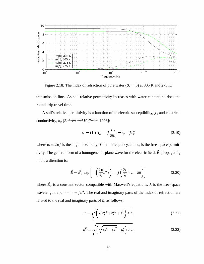
107

108

109

1010

1011

0

2

4

6

8

10

refr

activ

e in

dex

of w

ater

frequency, Hz

Re[n], 305 KIm[n], 305 KRe[n], 275 KIm[n], 275 K

Figure 2.18: The index of refraction of pure water (σe 0) at 305 K and 275 K.

transmission line. As soil relative permittivity increases with water content, so does the

round–trip travel time.

A soil’s relative permittivity is a function of its electric susceptibility, χe and electrical

conductivity, σe [Bohren and Huffman, 1998]:

εr

1 χe j

σe

ωεo

ε r j ε r (2.19)

where ω 2π f is the angular velocity, f is the frequency, and εo is the free–space permit-

tivity. The general form of a homogeneous plane wave for the electric field,E, propagating

in the z direction is:

E

Eo exp

2πλ

n z j

2πλ

n z ω t (2.20)

where

Eo is a constant vector compatible with Maxwell’s equations, λ is the free–space

wavelength, and n n j n . The real and imaginary parts of the index of refraction are

related to the real and imaginary parts of εr as follows:

n

ε r2 ε r 2 ε r 2 (2.21)

n

ε r2 ε r 2 ε r 2 (2.22)

60

In general, χe is complex. Due to its highly polar molecular structure, pure water ex-

hibits a dielectric relaxation between 5 and 30 GHz [Debye, 1929; Cole and Cole, 1952].

Above this relaxation frequency, the water molecules do not rotate and the relative permit-

tivity (and refractive index) decreases. Figure 2.18 illustrates this relaxation at two different

temperatures [Stogryn, 1971]. Using (2.20) it can be shown that the phase (propagation)

velocity of an electromagnetic wave is up c n where c is the speed of light in a vac-

uum. Waves propagating through a medium are also attenuated according to the magnitude

of n . Hence waves traveling on the TDR transmission line, whose Fourier components

range from the tens of MHz to the tens of GHz, will exhibit dispersion due to the fre-

quency dependence of the real and imaginary parts of the refractive index. The degree of

dispersion depends primarily on two factors: the fraction and degree to which soil water

is held, or bound, to the soil matrix [De Loor, 1956; Hoekstra and Doyle, 1972]; and the

bulk soil electrical conductivity [Hoekstra and Delaney, 1974]. Both effects are not well

understood. Bulk soil electrical conductivity increases linearly with water content in most

soils [Rhoades et al., 1989]. There is still much debate on the nature of bound water [Grant

et al., 1957; Wang, 1980; Dobson et al., 1985; Or and Wraith, 1999; Hillhorst et al., 2001]

and its effect on TDR measurements, particularly in clayey soils [Dasberg and Hopmans,

1992; Dirksen and Dasberg, 1993]. As a result, no universal calibration for TDR exists.

TDR measurements are also affected by temperature. Pepin et al. [1995] noted that

since pure water relative permittivity decreases with temperature (Figure 2.18), soil mois-

ture can be overestimated at higher soil temperatures. Their simple refractive mixing model

did not take into account soil type and they found that measured temperature change was

not as great as predicted. For the soils tested, sand had the greatest change with tempera-

ture, while loam and peat were much less. Persson and Berndtsson [1998] also measured

TDR temperature dependence, taking note of the temperature dependence of electrical con-

ductivity. The soils with large surface areas, high clay contents, and high electrical con-

ductivity had positive temperature correction factors. The other soils (which were mostly

61

0 0.1 0.2 0.3 0.4

0

0.005

0.010

0.015

0.020

volumetric water content, m3 m−3

perio

d te

mp

corr

ectio

n, m

s °C

−1

0.31 sand, 0.29 clay0.23 sand, 0.19 clay0.69 sand, 0.05 clay0.97 sandproposed

Figure 2.19: Proposed WCR period temperature correction based on Seyfried and Murdock[2001].

sands) had negative correction factors, as predicted by the temperature dependence of pure

water. Wraith and Or [1999] measured TDR pulse travel time as a function of temperature

for four soils. They found that high surface area and low water content are conditions fa-

vorable for an increase in measured travel time with increasing temperature and speculated

there is a “release” of bound water with temperature in soils with low water contents and

in soils with high surface areas.

Seyfried and Murdock [2001] tested the CS615 model 8221-07 WCR in air, water,

sand, and three soils to evaluate its temperature dependence. They found that the WCR

is extremely precise. There is also a small but significant unique sensor bias that can be

measured and corrected. The WCR electronics by themselves exhibit a small but consistent

temperature effect of -0.000533 ms

C 1. Following their example, the raw WCR pulse

periods were corrected for the electronics temperature effect. Inter–sensor variability was

ignored since three WCRs were averaged together at each combination H and L and depth.

The corrected period, P, was then fit to a second–order polynomial:

P A C1 θv C2 θ2v (2.23)

where A, C1, and C2 were found by the method of least squares using the impedance probe

measurements. The parameter A was forced to be 0.760 ms as found by Seyfried and Mur-

62

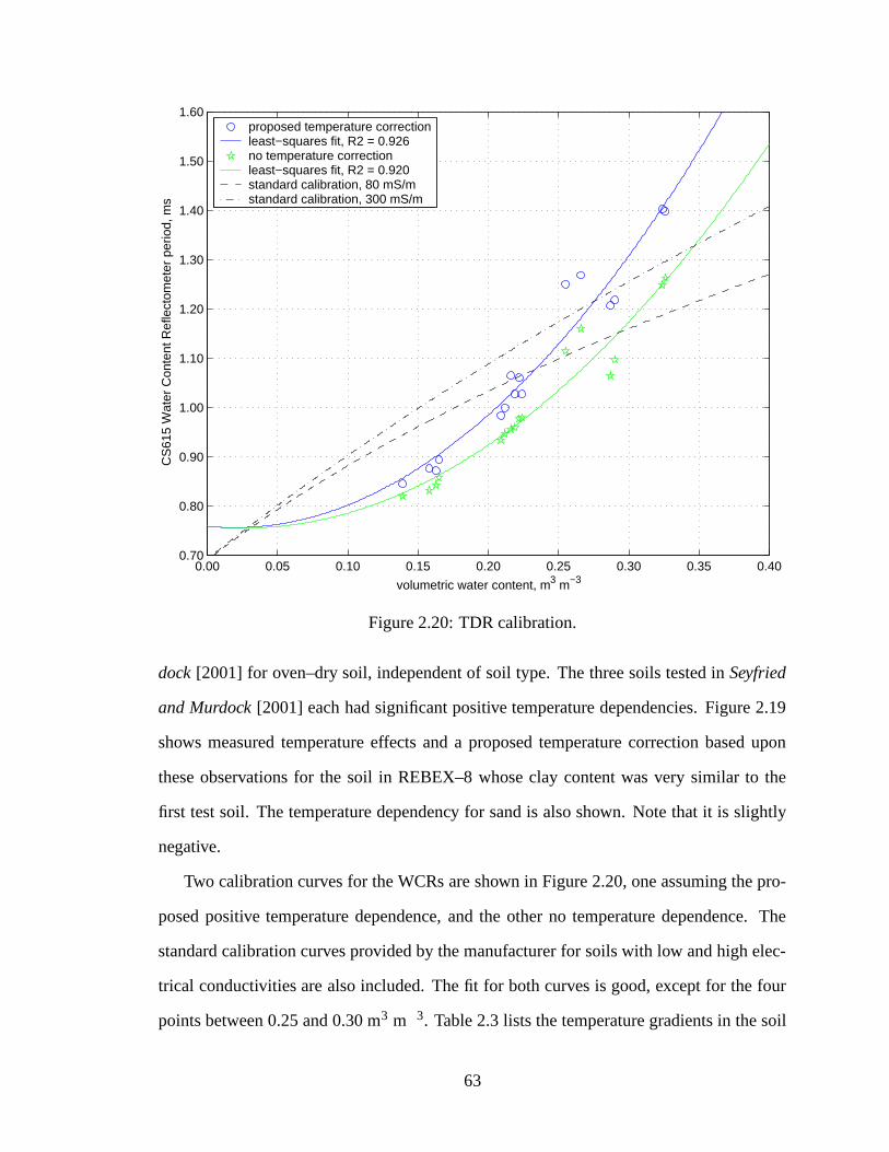
0.00 0.05 0.10 0.15 0.20 0.25 0.30 0.35 0.400.70

0.80

0.90

1.00

1.10

1.20

1.30

1.40

1.50

1.60

volumetric water content, m3 m−3

CS

615

Wat

er C

onte

nt R

efle

ctom

eter

per

iod,

ms

proposed temperature correctionleast−squares fit, R2 = 0.926no temperature correctionleast−squares fit, R2 = 0.920standard calibration, 80 mS/mstandard calibration, 300 mS/m

Figure 2.20: TDR calibration.

dock [2001] for oven–dry soil, independent of soil type. The three soils tested in Seyfried

and Murdock [2001] each had significant positive temperature dependencies. Figure 2.19

shows measured temperature effects and a proposed temperature correction based upon

these observations for the soil in REBEX–8 whose clay content was very similar to the

first test soil. The temperature dependency for sand is also shown. Note that it is slightly

negative.

Two calibration curves for the WCRs are shown in Figure 2.20, one assuming the pro-

posed positive temperature dependence, and the other no temperature dependence. The

standard calibration curves provided by the manufacturer for soils with low and high elec-

trical conductivities are also included. The fit for both curves is good, except for the four

points between 0.25 and 0.30 m3 m 3. Table 2.3 lists the temperature gradients in the soil

63

for eight impedance probe measurements, including three of the four poor points. (Recall

that each impedance probe measurement is the average of 70 individual measurements.)

The fourth, in H areas on day of year 145, was made just after a precipitation event and

hence is likely due to a sharp soil moisture gradient in the 0–6 cm soil layer. Table 2.3 also

includes day of year 185 when each H and L measurement fit the calibration curve well.

For day 143, during REBEX–8 when the vegetation cover was minimal, larger temperature

gradients were recorded than on day 185 during REBEX–8x. The temperature gradient

was also slightly larger in L areas where the poor calibration point was made. Day of year

270 was the only day on which impedance probe measurements were made in the after-

noon when temperature gradients tend to be greatest. Hence it is possible that temperature

gradients within the 0–6 cm layer caused the poor calibration points on days 143 and 270.

It is not known what caused the poor point on day 144.

Incident solar radiation, precipitation, and soil temperature at 1.5 cm, along with the

0–3 cm soil moisture in H areas during REBEX–8 using both the proposed temperature

correction from Figure 2.19 and no temperature correction is plotted in Figure 2.21. It ap-

pears that despite the high clay content of the soil, no temperature correction is warranted.

The curve with the proposed temperature dependence shows a large diurnal variation, with

unrealistic increases in soil moisture, particularly after each precipitation event. The use

of no temperature correction can also be justified by examining the taxonomic class of the

Table 2.3: Soil temperature gradients observed during impedance probe measurements.day of year time H / L θv, m3 m

3 soil IR 1.5 poor cal point?1.5 cm, K 4.5 cm, K

143 10:00 H 0.22 1.4 3.4 no143 10:00 L 0.27 1.6 3.3 yes144 8:40 H 0.22 -0.5 -0.2 no144 8:40 L 0.26 -0.8 -0.2 yes185 10:00 H 0.16 0.2 0.4 no185 10:00 L 0.22 0.3 0.2 no270 16:00 H 0.29 -0.3 1.9 yes270 16:00 L 0.32 0.1 1.5 no

64

0

500

1000

sola

r, W

m−2

0

2.0

4.0

prec

ip, m

m

10

20

30

soil

tem

p, °C

137 138 139 140 141 142 143 144 145 1460.18

0.22

0.26

0.30

0.34

soil

moi

stur

e, m

3 m−

3

day of year, 2001

positive temperature dependenceno temperature dependence

Figure 2.21: Solar radiation, precipitation, soil temperature at 1.5 cm, and 0–3 cm soilmoisture in H areas during REBEX–8. Local Daylight Time.

soils in question. The three soils in Seyfried and Murdock [2001] occur in arid climates and

all have high cation exchange capacities (CECs), or in other words, high electrical conduc-

tivity. The Lenawee silty clay loam at the experiment site (28.9% clay content), on the other

hand, exists in a more humid climate which tends to wash out salts, and as a result has a

low CEC. It is described as a fine, mixed, nonacid, mesic Mollic Epiaquepts [USDA–NRCS

Official Soil Series Descriptions, http://soils.usda.gov/classification/main.htm]. The mixed

minearology indicates that there is not one dominant type of clay that would favor a high

CEC. Although high clay content favors a positive temperature dependence, the type of

clay and its charge is equally important [personal communication, Sally Logsdon, USDA–

ARS, 2002]. For the soil in REBEX–8, any positive temperature dependence is probably

insignificant, or in any case balanced by the negative free water change with temperature.

65

0.10 0.15 0.20 0.25 0.30 0.35 0.400.10

0.15

0.20

0.25

0.30

0.35

0.40

ThetaProbe volumetric water content, m3 m−3

Wat

er C

onte

nt R

efle

ctom

eter

vol

umet

ric w

ater

con

tent

, m3 m

−3

Figure 2.22: Comparison of 0–6 cm volumetric soil water content measured by theThetaProbe with the average of 0–3 cm and 3–6 cm volumetric soil water content mea-sured by the Water Content Reflectometers.

For no temperature correction due to clay content, the values of the parameters in (2.23)

were A 0 760, C1 0 295, and C2

5 584. The accuracy of WCR measurements are

estimated to be 0 02 m3 m 3 based upon the uniformity of the site. Their precision is

0 01 m3 m 3.

A comparison of 0–6 cm volumetric soil water content measured by the ThetaProbe

with the average of 0–3 cm and 3–6 cm volumetric soil water content measured by the

Water Content Reflectometers with no temperature correction is shown in Figure 2.22. The

solid line is the one–to–one line.

66

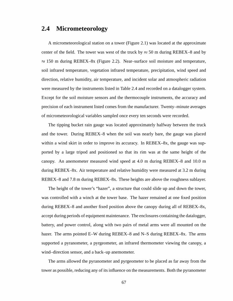
2.4 Micrometeorology

A micrometeorological station on a tower (Figure 2.1) was located at the approximate

center of the field. The tower was west of the truck by 50 m during REBEX–8 and by

150 m during REBEX–8x (Figure 2.2). Near–surface soil moisture and temperature,

soil infrared temperature, vegetation infrared temperature, precipitation, wind speed and

direction, relative humidity, air temperature, and incident solar and atmospheric radiation

were measured by the instruments listed in Table 2.4 and recorded on a datalogger system.

Except for the soil moisture sensors and the thermocouple instruments, the accuracy and

precision of each instrument listed comes from the manufacturer. Twenty–minute averages

of micrometeorological variables sampled once every ten seconds were recorded.

The tipping bucket rain gauge was located approximately halfway between the truck

and the tower. During REBEX–8 when the soil was nearly bare, the gauge was placed

within a wind skirt in order to improve its accuracy. In REBEX–8x, the gauge was sup-

ported by a large tripod and positioned so that its rim was at the same height of the

canopy. An anemometer measured wind speed at 4.0 m during REBEX–8 and 10.0 m

during REBEX–8x. Air temperature and relative humidity were measured at 3.2 m during

REBEX–8 and 7.8 m during REBEX–8x. These heights are above the roughness sublayer.

The height of the tower’s “hazer”, a structure that could slide up and down the tower,

was controlled with a winch at the tower base. The hazer remained at one fixed position

during REBEX–8 and another fixed position above the canopy during all of REBEX–8x,

accept during periods of equipment maintenance. The enclosures containing the datalogger,

battery, and power control, along with two pairs of metal arms were all mounted on the

hazer. The arms pointed E–W during REBEX–8 and N–S during REBEX–8x. The arms

supported a pyranometer, a pyrgeometer, an infrared thermometer viewing the canopy, a

wind–direction sensor, and a back–up anemometer.

The arms allowed the pyranometer and pyrgeometer to be placed as far away from the

tower as possible, reducing any of its influence on the measurements. Both the pyranometer

67

and pyrgeometer were ventilated. Negative values of irradiance recorded by the pyranome-

ter at night due to different cooling rates between the dome and detector [Dutton et al.,

2001] were set to zero. Case temperature corrections were made to the pyrgeometer using

the case thermistor measurement and not the optional voltage output. Dome temperature

was not measured and hence a correction was not made. This correction is small in general

[personal communication, Thomas Kirk, The Eppley Laboratory, 2002] and strongly de-

pendent on each pyrgeometer’s unique temperature–dependent calibration factor [Fairall

et al., 1998; Reda et al., 2002]. This calibration factor was not known and assuming an

average value would not have improved the measurement accuracy.

2.4.1 Infrared Thermometers

An infrared (IR) thermometer was positioned approximately 1 m above the canopy and

pointed at nadir. An identical IR thermometer underneath the canopy approximately 20 cm

above the ground and pointed at nadir measured the soil surface temperature. The IR ther-

mometers consist of two thermocouples: one that measures the detector temperature; and

another that measures the sensor body temperature used to correct the detector temperature.

The thermocouple measurements were subject to errors in: the reference junction temper-

ature; deviations in the thermocouple output from published standards; the thermocouple

voltage measurement; and the datalogger polynomial approximation [Campbell Scientific,

Inc., 2001]. A thermistor was used to measure the reference junction of the thermocou-

ples. This thermistor has a

0 2 K interchangeability error and a

0 1 K polynomial error,

resulting in a total accuracy error of

0 3 K. The temperature difference between the ther-

mistor (placed on the wiring panel of the datalogger) and the actual temperature of the

reference junctions (on the panel of a multiplexor) is small and can be neglected. since

the datalogger and multiplexor were approximately 10 cm apart within the same enclosure.

Deviations of the actual thermocouple wire performance to published standards are about

0 1 K. The accuracy of the datalogger voltage measurements and the polynomial relating

68

thermocouple emf to temperature are each

0 01 K. The manufacturer’s estimate of error

with sensor body temperature correction is

0 3 K. All of these errors add up to a total

accuracy of

0 7 K or less. The manufacturer lists the precision of the instrument as 0.05

K between 285 and 310 K. Precision is also affected by the voltage measurement accuracy

and changes in the reference thermistor temperature. All in all, the precision of the IR

thermometers is 0 1 K.

In addition to the errors associated with the instrument itself, there is also an error when

the object under view has an emissivity different from unity. Although the IR emissivity

of the soil changes with roughness and water content, the space within the lower canopy

is essentially a blackbody cavity after the fraction of cover has reached unity. As a result,

changes in soil emissivity are of no consequence and the radiometric temperature mea-

sured by the IR thermometer is close to the true radiometric temperature, which closely

approximates the thermodynamic temperature of the soil surface. On the other hand, de-

spite the fact that the emissivity of a continuous vegetation canopy is between 0.98 and 0.99

[Campbell and Norman, 1998], emission from the sky at IR wavelengths is considerably

different than emission from the canopy. At microwave wavelengths, sky emission is small

enough to be considered negligible. This is not the case at IR wavelengths and reflected

sky brightness should be considered.

A vegetation canopy can be modeled as a Lambertian (perfectly rough) surface. To

find the expected difference between the radiometric temperature measured by the IR ther-

mometer above the canopy and the true radiometric temperature of the canopy, consider a

Lambertian surface of temperature Ts 300 K and emissivity es. The irradiance, I, emitted

by this surface is:

I es IBs 1 es Isky (2.24)

where IBs is the blackbody irradiance of the surface and Isky is the downwelling sky irradi-

ance. Since emission from a Lambertian surface is independent of angle,

I π R (2.25)

69

where R is the radiance of the surface. The radiometric temperature of the surface is a

measure of this radiance R. Here the terms irradiance and radiance, instead of power density

and brightness, have been used in order to follow the terminology used in the thermal

IR remote sensing literature (see Norman and Becker [1995]). The units of irradiance

(also called radiant flux density) and radiance are W m 2 and W m

2 sr 1, respectively.

Although true for all wavelengths, in the following discussion the irradiances I, IBs, and

Isky and the radiance R are all considered to be within the band of the IR thermometer, 6.5

to 14 µm.

If sky irradiance and irradiance from the surface were the same, then the emissivity of

the surface is of no consequence and I IBs (as for the IR thermometer below the canopy).

In reality, Isky IBs so that I IBs. In other words, the radiometric temperature of this

Lambertian surface as measured by the IR thermometer will always be less than its true

radiometric temperature. Furthermore, sky irradiance is greatest on cloudy days due to the

large amount of water vapor in the atmosphere. Hence the difference between I and IBs (the

measured and true radiometric temperature of the surface) will be largest on clear days.

Sky irradiance in the 4 to 50 µm band, Isky 4 50, was measured by the pyrgeometer. Sky

irradiance in the IR thermometer’s wavelength band, Isky, can be calculated as follows. The

emissivity of the sky over all wavelengths, esky ∞, can be approximated

esky ∞

Isky 4 50

σ T 4sky

(2.26)

where: σ is the Stefan–Boltzmann constant; and Tsky is the effective emitting temperature

of the sky, both within the band of the IR thermometer and at all wavelengths. This approx-

imation can be made because the irradiance above 50 µm is small and can be neglected. For

a clear sky [Brutsaert, 1984],

esky ∞ 1 72

wair

Tair 1 7

(2.27)

where wair and Tair are the water vapor pressure (in kPa) and the air temperature (in K),

respectively, near the surface. For clear days, the effective temperature of the sky can be

70

7 8 9 10 11 12 13 140

5

10

15

20

25

30

wavelength, µm

spec

tral

irra

dian

ce, W

m−

2 µm

−1

wavelength band of IR thermometer

clear sky288 K blackbody

Figure 2.23: Spectral irradiance of a clear sky of effective temperature Tsky 288 K within

the band of the IR thermometer. Approximated from Figure 10.6 of Campbell and Norman[1998]. Blackbody irradiance is also plotted.

found from (2.26) and (2.27):

Tsky

Isky 4 50

1 72σwair

Tair 1 7 1 4

(2.28)

All of the variables in (2.28) were measured in REBEX–8 and –8x: Isky 4 50 by the pyrge-

ometer; and wair and Tair by the air temperature / relative humidity probe at 7.8 m.

The emissivity of the sky in the band of the IR thermometer, esky, was found using the

graph of clear sky spectral irradiance versus wavelength when Tsky 288 K in Figure 10.6

of Campbell and Norman [1998]. An approximation of the 6.5 to 14 µm band of this figure

is reproduced here in Figure 2.23. Integrating the total irradiance from the atmosphere in

the 6.5 to 14 µm band and dividing by the irradiance of a 288 K blackbody in the same

71

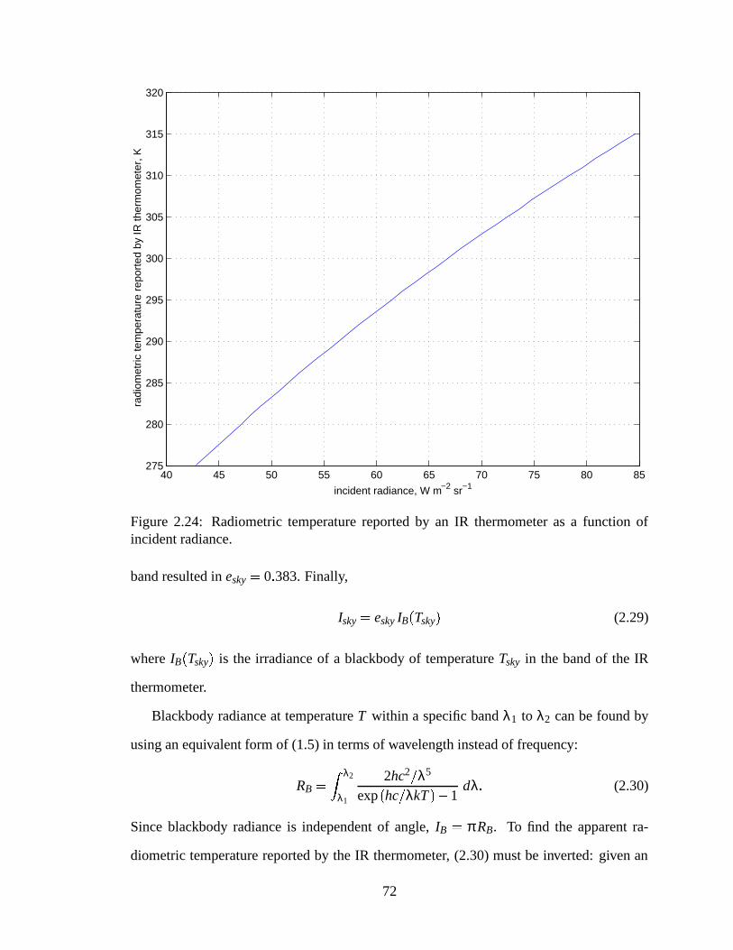
40 45 50 55 60 65 70 75 80 85275

280

285

290

295

300

305

310

315

320

incident radiance, W m−2 sr−1

radi

omet

ric te

mpe

ratu

re r

epor

ted

by IR

ther

mom

eter

, K

Figure 2.24: Radiometric temperature reported by an IR thermometer as a function ofincident radiance.

band resulted in esky 0 383. Finally,

Isky esky IB

Tsky (2.29)

where IBTsky is the irradiance of a blackbody of temperature Tsky in the band of the IR

thermometer.

Blackbody radiance at temperature T within a specific band λ1 to λ2 can be found by

using an equivalent form of (1.5) in terms of wavelength instead of frequency:

RB λ2

λ1

2hc2 λ5

exphc λkT 1

dλ (2.30)

Since blackbody radiance is independent of angle, IB π RB. To find the apparent ra-

diometric temperature reported by the IR thermometer, (2.30) must be inverted: given an

72

incident radiance, a blackbody of what temperature would produce this radiance? The rela-

tionship between the radiometric temperature reported by the IR thermometer as a function

of incident radiance was computed numerically and is shown in Figure 2.24.

From analysis of downwelling solar radiation measured by the pyranometer, thirteen

clear sky days were identified during REBEX–8x. The coolest effective sky temperature,

Tsky, calculated for these clear days was 279 K. This occurred the morning of a microwave

radiometer calibration. Field notes confirm a clear sky that morning. The warmest effec-

tive sky temperature calculated for these clear days was 307 K. The maximum difference

between R and RB in (2.25) will be for the lowest possible value of es and the lowest value

of Tsky. For a Lambertian surface of temperature Ts 300 K, emissivity es

0 98, and

sky effective temperature Tsky 279 K, the radiometric temperature reported by an IR ther-

mometer would be 299.1 K. The smallest difference between R and RB in (2.25) will be for

the highest possible value of es and the highest value of Tsky. For a Lambertian surface of

temperature Ts 300 K, emissivity es

0 99, and sky effective temperature Tsky 307 K,

the radiometric temperature reported by an IR thermometer would be 299.7 K. Hence, the

maximum difference between the actual radiometric temperature of the vegetation canopy

and the radiometric temperature reported by the IR thermometer is about 0.9 K. This dif-

ference will always be at least 0.3 K on clear sky days.

2.4.2 Soil Temperature

Soil temperature measurements at 1.5 and 4.5 cm were made with thermocouples and

thermistors, respectively. Four thermocouple measurements, made in adjacent rows, were

averaged together to measure soil temperature at 1.5 cm in both H and L areas. The ther-

mocouples were encased in metal rods less than 3 mm in diameter. They were subject to

the same thermocouple errors as the IR thermometers, resulting in an accuracy of

0 4 K

or less and a precision of 0 1 K. Each H and L measurement at 4.5 cm was the average

of 3 separate measurements made in adjacent rows.

73

2.4.3 Summary

Table 2.4 lists the accuracy and precision of instruments during REBEX–8 and –8x. In

some cases, more than one of the same type of instrument were used to measure a specific

variable. For these cases, a second row lists the accuracy and precision of the averaged

data on the plot–scale. For example, three 107 temperature probes were used to measure

4.5 cm soil temperature. If the accuracy of one probe is

0 2 K, then the accuracy of

the average of three of these probes is less than

0 2 3

0 1 K. The accuracy and

precision of individual CS615 Water Content Reflectometers were not determined. For the

vegetation IR temperature, only instrument, and not emissivity, errors are given.

74

Table 2.4: Accuracy and precision of instruments used in REBEX–8 and –8x. In some cases, more than one of the same type ofinstrument were used to measure a specific variable. For these cases, a second row lists the accuracy and precision of the averaged dataon the plot–scale.Instrument Manufacturer Variable Accuracy Precisionmicrowave radiometers Univ. of Michigan 1.4 GHz brightness

2 K 0.4–1.7 KThetaProbe ML2x Delta–T Devices 0–6 cm volumetric soil moisture

0 01 m3 m

3 0 02 m3 m

3

0 01 m3 m

3 0 01 m3 m

3

CS615 Water Content Reflectometers Campbell Scientific 0–3 & 3–6 cm vol. soil moisture

0 02 m3 m

3 0 01 m3 m

3

107 Temperature Probes Campbell Scientific soil temperature @ 4.5 cm

0 2 K 0 1 K

0 1 K 0 1 KTCAV Soil Thermocouple Probes Campbell Scientific soil temperature @ 1.5 cm

0 4 K 0 1 K

0 3 K 0 1 KTE525 Tipping Bucket Rain Gauge Texas Electronics precipitation

1%

0 3 mmPSP pyranometer Eppley downwelling solar radiation

1–2% 1 W m

2

PIR pyrgeometer Eppley downwelling atmospheric radiation

3% 1 W m

2

014A anemometer Met–One wind speed @ 10 m

1 5% 0 1 m s

1

HMP35C Air Temp. / RH Probe Vaisala air temperature @ 7.8 m

0 4 K 0 1 KHMP35C Air Temp. / RH Probe Vaisala relative humidity @ 7.8 m

2–3% RH 0 1% RHPrecision IR Thermocouple Transducers Apogee soil & vegetation IR temperature

0 7 K 0 1 K

75

CHAPTER 3

The Nature of Absorption, Emission, and VolumeScattering in Field Corn at 1.4 GHz

Chapter 3 begins with a discussion of the dielectric properties of a field corn canopy as

a function of orientation, both in azimuth and elevation. It also includes the procedure used

to show that the zero–order radiative transfer model is unable to predict the correct change

in brightness temperature with incidence angle unless some degree of scattering is allowed

and the canopy is considered to be anisotropic in elevation. Finally, a new semi–empirical

zero–order model is formulated for mature corn and the variation of its parameters with

incidence angle and polarization is discussed.

3.1 Row Anisotropy

Although spatially heterogeneous on meter scales due to the variable size of plant con-

stituents such as stems, leaves, and ears, a field corn canopy can be considered quasi–

continuous at 1.4 GHz [Ulaby et al., 1987] and hence treated as a single dielectric layer.

Dielectric anisotropy can result in the polarization of electromagnetic waves. As a result,

emitted brightness of anisotropic media can depend upon the propagation direction. Is a

field corn canopy anisotropic in azimuth at 1.4 GHz? Or, in other words, is the brightness

temperature a function of row direction?

Because of the significant row structure of field corn, it would seem so. The stems and

ears, essentially moist dielectric rods with thicknesses a significant fraction of the wave-

76

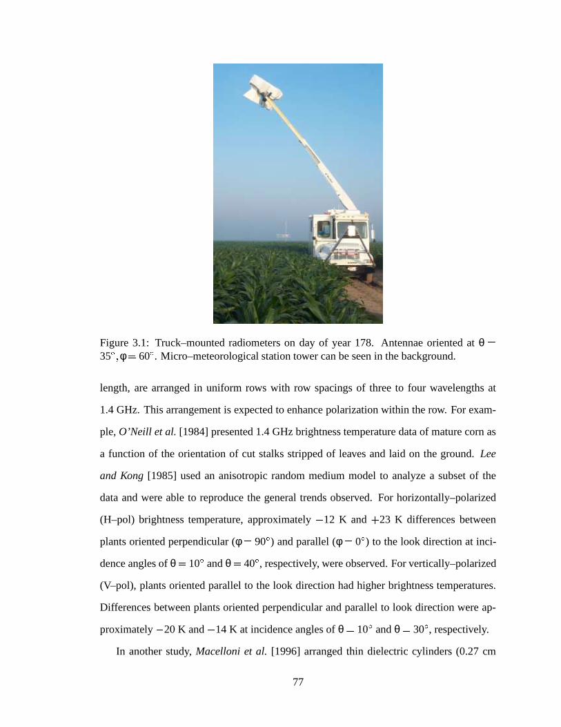
Figure 3.1: Truck–mounted radiometers on day of year 178. Antennae oriented at θ

35

φ 60

. Micro–meteorological station tower can be seen in the background.

length, are arranged in uniform rows with row spacings of three to four wavelengths at

1.4 GHz. This arrangement is expected to enhance polarization within the row. For exam-

ple, O’Neill et al. [1984] presented 1.4 GHz brightness temperature data of mature corn as

a function of the orientation of cut stalks stripped of leaves and laid on the ground. Lee

and Kong [1985] used an anisotropic random medium model to analyze a subset of the

data and were able to reproduce the general trends observed. For horizontally–polarized

(H–pol) brightness temperature, approximately 12 K and 23 K differences between

plants oriented perpendicular (φ 90

) and parallel (φ 0

) to the look direction at inci-

dence angles of θ 10

and θ 40

, respectively, were observed. For vertically–polarized

(V–pol), plants oriented parallel to the look direction had higher brightness temperatures.

Differences between plants oriented perpendicular and parallel to look direction were ap-

proximately 20 K and 14 K at incidence angles of θ 10

and θ 30

, respectively.

In another study, Macelloni et al. [1996] arranged thin dielectric cylinders (0.27 cm

77

6:20 7:45 8:21 8:59 9:48288

290

292

294

tem

pera

ture

, K

REBEX−8x3

soil

vegetation

6:20 7:45 8:21 8:59 9:48

264

266

268

270

272

274

276

278

280

brig

htne

ss te

mpe

ratu

re, K

LDT on day of year 229

φ = 60° 0° 15°30°60° 90° 60°

V−pol

H−pol

θ = 15°θ = 35°θ = 55°

Figure 3.2: Time sequence of H–pol and V–pol brightness temperature as a function ofangle with respect to row direction (φ) during REBEX–8x3. Errorbars of

NE∆T are

included. The measurements at φ 60

and θ 35

are circled. Soil temperature at1.5 cm and vegetation IR temperature are also plotted.

diameter, 20 cm length) in periodic rows on a reflecting background. At 10 GHz they

found: no difference in brightness temperature between φ 0

and φ 90

at θ 20

for

both vertical and horizontal polarizations; 12 K and 8 K difference for V– and H–pol,

respectively, at θ 30

; a 10 K and 8 K difference at θ 40

, and a 10 K and 6 K

difference at θ 50

. Although the frequency of observation was 10 GHz, the electrical

size of the dielectric cylinders used in this study is similar to the electrical size of stems

and ears at 1.4 GHz.

Only one direct measurement of the brightness temperature of a field corn canopy with

78

φ = 60o

θ = 15o,35o,55o

8:39− 8:57

φ = 90o

θ = 55o,35o,15o

8:59− 9:15

φ = 60o

θ = 35o

9:52 LDT

CALIBRATION

φ = 60o

θ = 35o

6:32 LDT

φ = 15o

θ = 15o,35o,55o

8:03− 8:19

φ = 30o

θ = 55o,35o,15o

8:21− 8:37

φ = 0o

θ = 55o,35o,15o

7:45− 8:01

CALIBRATION

Figure 3.3: Measurement procedure during REBEX–8x3.

respect to row direction has been reported. Brunfeldt and Ulaby [1986] observed a 10 K

difference between φ 90

and φ 0

for V–pol brightness temperature at 2.7 GHz for

a 5.5 kg m 2 vegetation column density corn crop. Row direction experiments were con-

ducted at several points during REBEX–8 and REBEX–8x (Figure 3.1). Measurements of

H–pol and V–pol brightness at 1.4 GHz collected during REBEX–8x3 for a mature corn

canopy (vegetation column density of 8.0 kg m 2) at several different angles with respect

to row direction and angles of incidence are plotted in Figure 3.2. These measurements

were made during a period of three and a half hours starting at 6:30 LDT (Local Daylight

Time) on day of year 229. During the previous night, the radiometers had been left record-

ing data at φ 60

and θ 35

. The last measurements at this position, at 6:32, are the first

two points on the left in Figure 3.2. See Figure 3.3 for a description of the measurement

procedure. Three measurements of brightness temperature, each separated by two minutes,

were made at each combination of φ and θ in order to verify the measurement precision.

See Table 3.1 for a description of footprint size relative to row spacing.

The general increase in brightness temperatures over the measurement period evident

in Figure 3.2 was due to slowly changing soil and vegetation temperatures. In order to

remove this effect, the three φ 60

and θ 35

points for both H–pol and V–pol at 6:32,

8:49, and 9:52 LDT were used to construct two second–degree polynomials. These two

79

Table 3.1: Radiometer footprint size in terms of the number of rows of corn that would lieinside of the footprint. Maximum canopy height was 3.0 m.

φ 0

φ 90

z 0 m z 3.0 m z 0 m z 3.0 mθ 15

6 rows 4 rows 6 rows 5 rowsθ 35

6 rows 4 rows 9 rows 7 rowsθ 55

5 rows 3 rows 15 rows 10 rows

polynomials are an approximation of the change in brightness temperature over time at φ

60

and θ 35

for each polarization. Subtracting these polynomials from the measured

brightness temperatures revealed the variation in microwave brightness as a function of

row direction, referenced to the brightness temperature at φ 60

. In order to remove the

temperature change effects from the θ 15

and θ 55

data, the relevant polynomial,

according to polarization, was shifted either up or down in order to match the recorded

data at φ 60

and θ 15

and 55

. In using this compensation procedure derived at

θ 35

the assumption is made that the weighting of soil and vegetation temperatures is

the same at θ 15

and θ 55

. This is not exactly true. At θ 15

, the soil contribution

to the brightness temperature is slightly larger than at θ 35

, while at θ 55

, the soil

contribution is slightly smaller. In either case, the vegetation contribution dominates and

the change in relative contribution is small. Figures 3.4 and 3.5 present the results.

Surprisingly, field corn brightness at 1.4 GHz was not a strong function of angle with

respect to row direction until senescence. As the corn was growing and when it was fully

mature, the observed variation in brightness temperature with φ was very small, about 1

to 2 K. Since there were no obvious patterns in these variations, they were probably the

result of radiometer precision, the vegetation and soil compensation method, and soil and

canopy variability. Despite the absence of a complete set of data for REBEX–8x1 and –

8x2, there is no reason to doubt that H–pol brightness temperature is also independent of

row direction during this period. When the corn was fully senescent in early October dur-

ing REBEX–8x4, a consistent pattern did emerge at all incidence angles: H–pol brightness

temperatures were highest parallel to the rows at φ 0

, while V–pol brightness temper-

80

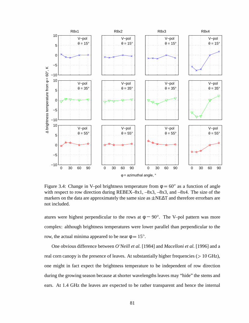
−10

−5

0

5

10

θ = 15°

R8x1

V−pol

−10

−5

0

5

10

θ = 35°V−pol

∆ br

ight

ness

tem

pera

ture

from

φ =

60°

, K

0 30 60 90−10

−5

0

5

10

θ = 55°V−pol

φ = azimuthal angle, °

θ = 15°

R8x2

V−pol

θ = 35°V−pol

0 30 60 90

θ = 55°V−pol

θ = 15°

R8x3

V−pol

θ = 35°V−pol

0 30 60 90

θ = 55°V−pol

θ = 15°

R8x4

V−pol

θ = 35°V−pol

0 30 60 90

θ = 55°V−pol

Figure 3.4: Change in V–pol brightness temperature from φ 60

as a function of anglewith respect to row direction during REBEX–8x1, –8x3, –8x3, and –8x4. The size of themarkers on the data are approximately the same size as

NE∆T and therefore errorbars are

not included.

atures were highest perpendicular to the rows at φ 90

. The V–pol pattern was more

complex: although brightness temperatures were lower parallel than perpendicular to the

row, the actual minima appeared to be near φ 15

.

One obvious difference between O’Neill et al. [1984] and Macelloni et al. [1996] and a

real corn canopy is the presence of leaves. At substantially higher frequencies ( 10 GHz),

one might in fact expect the brightness temperature to be independent of row direction

during the growing season because at shorter wavelengths leaves may “hide” the stems and

ears. At 1.4 GHz the leaves are expected to be rather transparent and hence the internal

81

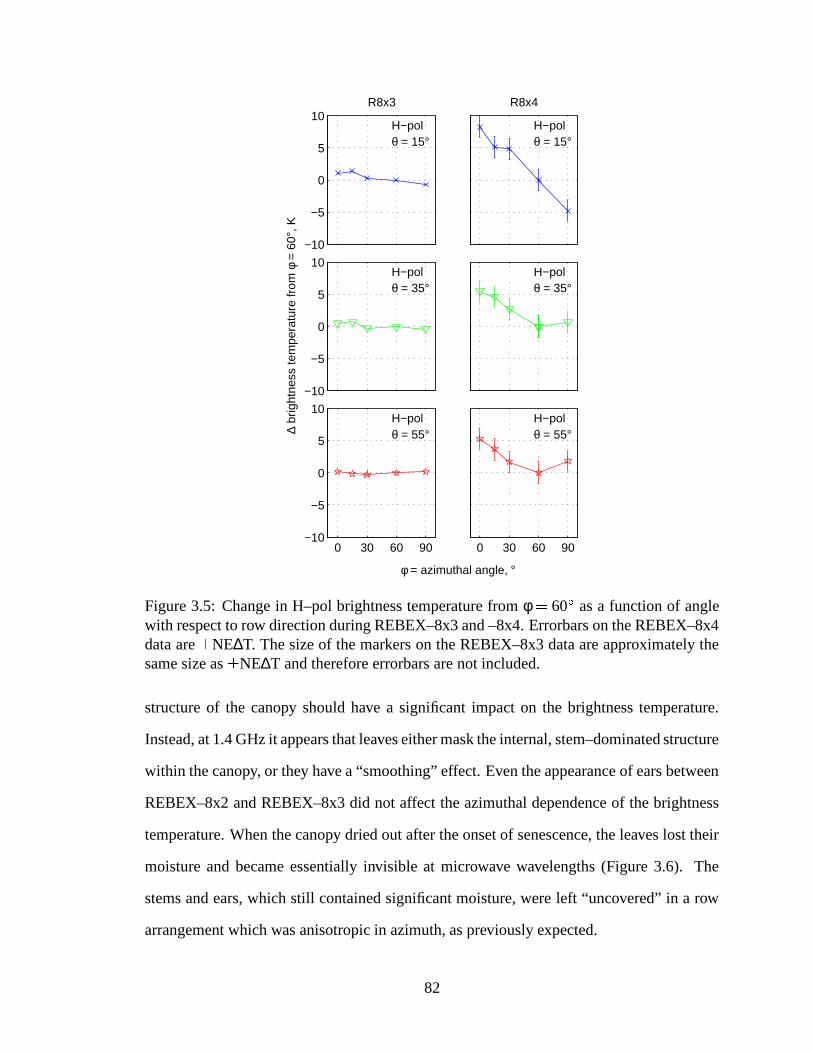
−10

−5

0

5

10

θ = 15°

R8x3

H−pol

−10

−5

0

5

10

∆ br

ight

ness

tem

pera

ture

from

φ =

60°

, Kθ = 35°H−pol

0 30 60 90−10

−5

0

5

10

θ = 55°

φ = azimuthal angle, °

H−pol

θ = 15°

R8x4

H−pol

θ = 35°H−pol

0 30 60 90

θ = 55°H−pol

Figure 3.5: Change in H–pol brightness temperature from φ 60

as a function of anglewith respect to row direction during REBEX–8x3 and –8x4. Errorbars on the REBEX–8x4data are

NE∆T. The size of the markers on the REBEX–8x3 data are approximately the

same size as

NE∆T and therefore errorbars are not included.

structure of the canopy should have a significant impact on the brightness temperature.

Instead, at 1.4 GHz it appears that leaves either mask the internal, stem–dominated structure

within the canopy, or they have a “smoothing” effect. Even the appearance of ears between

REBEX–8x2 and REBEX–8x3 did not affect the azimuthal dependence of the brightness

temperature. When the canopy dried out after the onset of senescence, the leaves lost their

moisture and became essentially invisible at microwave wavelengths (Figure 3.6). The

stems and ears, which still contained significant moisture, were left “uncovered” in a row

arrangement which was anisotropic in azimuth, as previously expected.

82

R8 R8x1 R8x2 R8x3 R8x40

2

4

6

8

wat

er c

olum

n de

nsity

, kg

m−

2 cobsstemsleaves

Figure 3.6: Distribution of water column density during each REBEX.

3.2 Volume Scattering

The stems and ears of field corn have sizes of the same order of the wavelength, and

hence some degree of scattering within the canopy will occur. What is the nature of this

volume scattering? Despite their arrangement in well–defined rows, the location of scat-

terers relative to one another is random with respect to the wavelength. As a result, the

electric field at any one point within the canopy is the superposition of waves that have no

coherence with each other. In the soil, changes in the dielectric constant due to changes in

moisture, as long as they are gradual and not abrupt, also destroy wave coherence. Under

these conditions, it is appropriate to use incoherent radiative transfer to model the mi-

crowave brightness.

Within a medium, the incremental change in brightness temperature at each point is the

sum of three effects [Ulaby et al., 1981-1986]:

dTBs κe TB

s ds κa T ds κs

4π

4πψ

s s TB

s dΩ ds (3.1)

First, brightness in the s direction is attenuated in proportion to the medium’s extinction

coefficient, κe. Extinction is due to both absorption by the medium (κa) and scattering

by particles within the medium (κs). Second, the medium emits according to its physical

temperature, T , in order to maintain thermodynamic equilibrium. Finally, brightness from

all other directions s is scattered into the s direction according to the normalized phase

83

function ψs s .

In the simplest case, a vegetated surface can be modeled as a single isothermal layer

of vegetation with diffuse boundaries over a soil half space. After applying appropriate

boundary conditions, the zero–order solution of (3.1) can be written

TB TBsoil TBcanopy TBcanopy (3.2)

where

TBsoil Tsoil

1 Rsoil L (3.3)

TBcanopy 1 α

1 L Tcanopy (3.4)

TBcanopy 1 α

1 L Tcanopy Rsoil L (3.5)

TBsoil represents the soil contribution to the total brightness temperature. TBcanopy and

TBcanopy represent upwelling and reflected downwelling emission from the vegetation

canopy, respectively. Tsoil is the effective soil temperature; Rsoil , an effective reflectiv-

ity of the soil surface; L exp τ cosθ , the transmissivity of the vegetation layer; τ

κa κs h κeh, the canopy optical depth; h, the canopy height; α κs

κe, the single-

scattering albedo; and Tcanopy, the canopy temperature. Reflected sky brightness, which is

only a few Kelvin at 1.4 GHz, is neglected. Rsoil is a function of volumetric water content.

τ and α are determined primarily by the structure and water content of the canopy.

The zero–order solution assumes weak scattering within the canopy: either ψs s 0,

which means little power is scattered into the forward direction; κs is very small, meaning

either the number or the extinction cross section of the scatterers is small; or α 1, such

that κs κa. A non–zero single-scattering albedo produces a lower effective vegetation

temperature to account for limited volume scattering. Many researchers in the past have

used this model for field corn [Jackson et al., 1982; Mo et al., 1982; Brunfeldt and Ulaby,

1986; Jackson and O’Neill, 1990; O’Neill et al., 1996; Jackson et al., 1997; Crosson et al.,

2002] under the assumption that scattering is small at 1.4 GHz. Is this indeed true? Can a

84

Table 3.2: Canopy and soil properties during brightness temperature measurements at φ

60

and θ 15

, 35

, and 55

.R8 -x1 -x2 -x3 -x4

IR vegetation temp, K 284 292 290 290 278IR soil surface temp, K 284 293 290 291 278soil temp @ 1.5 cm, K 285 293 289 291 281soil temp @ 4.5 cm, K 285 293 291 291 283vol soil moist 0-3 cm, m3 m

3 0.22 0.13 0.10 0.15 0.25vol soil moist 3-6 cm, m3 m

3 0.25 0.20 0.18 0.19 0.28

field corn canopy be considered a weakly–scattering canopy at 1.4 GHz so that (3.2) can

be used?

When considering a scattering layer over a homogeneous half–space, England [1975]

showed that scatter–induced change in brightness temperature can be tens of Kelvin. Vol-

ume scattering is a function of the dielectric contrast between the scatterers in the medium,

the dielectric loss of the scatterers, the size of scatterers relative to wavelength, and the

fraction of volume filled by the scatterers. If the dielectric constant of the half–space is not

significantly larger than the dielectric constant of the scattering layer (as in the case of a

vegetation layer over a moist soil half–space) the presence of scatterers reduces the bright-

ness temperature. This phenomena is called scatter darkening. For example, Liou et al.

[1999] observed scatter darkening in prairie grass. They were able to accurately model

19 GHz brightness with a purely absorptive volume emission model, but model predictions

of 37 GHz brightness were too high.

Most of the experimental validation of the zero–order model has been at incidence

angles close to nadir where the effects of scattering in the canopy are least. One way to

test the assumption of weak scattering is to examine the change in brightness temperature

with incidence angle. As the impact of the canopy on the microwave brightness increases

at progressively larger angles of incidence, can the zero–order solution correctly recreate

what is observed experimentally?

Observed 1.4 GHz brightness temperature from each REBEX at φ 60

and incidence

angles of θ 15

, 35

, and 55

were compared with the predictions of the zero–order model

85

(3.2). These measurements were made near dawn as part of the row direction experiments.

All three incidence angles were measured within a period of less than 20 minutes. Recorded

canopy temperatures, soil temperatures, and moisture are listed in Table 3.2. The average

of recorded vegetation and soil IR temperatures were used for Tcanopy. Tsoil was computed

using the parameterization of Wigneron et al. [2001]:

Tsoil T∞

Tsur f T∞ θv

w0 BT (3.6)

where: T∞ is a deep soil temperature, typically at 50 cm; Tsur f is the soil temperature near

the surface; θv is the soil surface water content; and w0 and BT are parameters which de-

pend on the choice of depth for Tsur f and θv. This is a variation the model proposed by

Choudhury et al. [1982] parameterized specifically for the agricultural fields in which they

collected their data. The soil texture of these fields (62% silt, 11% sand, and 27% clay)

closely matches that of REBEX–8 (55% silt, 16% sand, and 29% clay). Soil tempera-

ture at 50 cm was not measured during REBEX–8 but during the previous summer in a

nearly identical corn field planted and cultivated using the same practices 1 km north of

the REBEX–8 site. At this depth, soil temperature does not vary diurnally and is almost

constant for periods of weeks at a time. Depths of 1.5 cm and 0–3 cm were chosen for Tsur f

and θv, respectively, resulting in w0 0 794 and BT

0 258. In all cases, Tsoil and soil

temperature measured at 1.5 cm were within 2 K. A dielectric model [Dobson et al., 1985]

and recorded 0–3 cm soil moisture were used to calculate the specular reflectivity of the

soil at the site. The optical depth was computed using the model of Jackson et al. [1982]

and Schmugge and Jackson [1992] which relates τ directly to the water column density,

Mw, the mass of water in the vegetation per square meter:

τ bMw (3.7)

A value of b 0 115, appropriate for corn at 1.4 GHz when α 0, was used [Jackson and

O’Neill, 1990]. Figures 3.7 and 3.8 compare the observations with the model results.

As an aside, note that the temperatures listed in Table 3.2 are nearly uniform, especially

86

R8 R8x3 R8x4

160

180

200

220

240

260

280

H−pol

(a) OBSERVED

brig

htne

ss te

mpe

ratu

re, K

θ = 15°θ = 35°θ = 55°

R8 R8x3 R8x4

160

180

200

220

240

260

280

H−pol

(b) specular

R8 R8x3 R8x4

160

180

200

220

240

260

280

H−pol

(c) rough

R8 R8x3 R8x4

160

180

200

220

240

260

280

(d) rough, α > 0

H−pol

Figure 3.7: Observed (a) and modeled (b, c, and d) H–pol brightness temperature at φ 60

during REBEX–8, –8x3, and –8x4. For the model results: (b), the soil surface is specular;(c), the soil surface is rough; and (d), the soil surface is rough and α 0.

during REBEX–8, REBEX–8x1, and –8x3. Thus any effect of temperature gradients within

the canopy and soil on the microwave brightness was negligible. The emissivity of the

land surface, e, defined as the ratio of brightness temperature to physical temperature, is

approximately e 269 K 291 K 0 92 for H–pol and e 277 K 291 K 0 95 for

V–pol during REBEX–8x3. The V–pol emissivity during REBEX–8x1 was also about 0.95.

For H–pol, three different versions of the zero–order model were used to illustrate the

effect of different physical processes on the brightness temperature. In the first version, part

(b) of Figure 3.7, the soil surface was modeled as specular and the single–scattering albedo,

α, was set to zero. In comparison to part (a), the observed H–pol brightness temperature,

87

it is obvious that the REBEX–8 predictions are too low, but the change with incidence

angle θ is correct. When the amount of vegetation is small, the total brightness temperature

is dominated by (3.3). The measurements and model both followed the Fresnel law: the

brightness temperature was highest near nadir and gradually decreased as the incidence

angle increased.

When the canopy was mature during REBEX–8x3, the zero–order model no longer

correctly predicted the change in H–pol brightness temperature as a function of θ. This

is illustrated in part (a) and (b) of Figure 3.7 by the lines linking the REBEX–8 and –8x3

brightness temperatures. In the model predictions, the lines cross. At large water column

densities, canopy emission composes a higher fraction of the total brightness temperature

than emission from the soil. As the path length through the canopy increases at larger angles

of θ, the zero–order model predicts canopy emission to increase at a rate which out paces

the decrease in soil microwave brightness. The result is that in weakly scattering vegetation

canopies, microwave brightness should increase with θ when the water column density

is large. This is opposite what was observed. For the field corn canopy, the brightness

temperature decreased with θ, a sign of scatter darkening in the canopy.

In the second version of the zero–order model, part (c) of Figure 3.7, the soil was

modeled more realistically as rough surface using the model [Choudhury et al., 1979; Wang

et al., 1980a]

Rrough Rspec exp

hs (3.8)

where Rspec is the specular reflectivity and hs is an effective roughness parameter. hs was

computed using the formulation of Wigneron et al. [2001]:

hs A θv

B σs

lc C (3.9)

where: A 0 5761, B 0 3475, and C 0 4230 are empirical parameters; θv is the

volumetric soil moisture in m3 m 3 of the 0–3 cm soil layer; σs is the standard deviation of

soil surface height; and lc is the soil surface correlation length. This empirical formulation

88

of hs was made using data collected in bare agricultural fields of varying roughness at

incidence angles of θ 10

20

30

and 40

. Soil surface roughness was measured with a

laser profiler the previous summer in late August. Four meter–long transects perpendicular

to row direction were used to calculate a σs of 14 mm and a lc of 85 mm, which are

representative of the conditions during REBEX–8x3. According to Oh and Kay [1998],

surface segments totaling 40σs and 200lc must be used to accurately characterize these

surface parameters. While this condition was satisfied for σs, lc must be considered a

rough estimate. These values are similar to those measured by Wigneron et al. [2001] for

their field 18 with σs 19 mm and lc 66 mm. Again, the soil texture of the fields in

Wigneron et al. [2001] was close to the texture of the REBEX–8 field.

As expected, the REBEX–8 model predictions increased since the emissivity of a rough

surface is higher than that of a smooth one. The predictions were more in line with the

observations of part (a). The large difference in observed and modeled brightness tem-

peratures at θ 55

is likely due to different soil roughness conditions during REBEX–8

(before cultivation) and REBEX–8x (after cultivation). The range of data used to calibrate

the model did not reach θ 55

although Wang et al. [1980a] observed that a soil sur-

face with significant row structure did not change the variation of brightness temperature

with incidence angle significantly at H–pol. Although the absolute change in H–pol bright-

ness temperature with θ was not correctly predicted by the model, the relative change in

brightness, in keeping with the Fresnel law, was the same: brightness still decreased as the

incidence angle increased.

In the the third version of the zero–order model, part (d) of Figure 3.7, α is set to

0.03 [Jackson and O’Neill, 1990] and the soil surface remains rough. A non–zero single–

scattering albedo did decrease the difference between the three incidence angles, but the

modeled change with incidence angle was still opposite that of the observations. Neither a

rough soil surface nor the addition of a non–zero single–scattering albedo altered the rel-

ative position of the predictions. Furthermore, the modeled change with incidence angle

89

R8x1 R8x2 R8x3 R8x4

240

250

260

270

280

290 V−pol

(a) OBSERVED

brig

htne

ss te

mpe

ratu

re, K

θ = 15°θ = 35°θ = 55°

R8x1 R8x2 R8x3 R8x4

240

250

260

270

280

290 V−pol

(b) specular

R8x1 R8x2 R8x3 R8x4

240

250

260

270

280

290 V−pol

(c) rough

R8x1 R8x2 R8x3 R8x4

240

250

260

270

280

290 V−pol

(d) rough, R ≠ f(θ)

R8x1 R8x2 R8x3 R8x4

240

250

260

270

280

290 V−pol

(e) rough, R ≠ f(θ), α > 0

Figure 3.8: Observed (a) and modeled (b, c, d, and e) V–pol brightness temperature atφ 60

during REBEX–8x1, –8x2, –8x3, and –8x4. For the model results: (b), the soilsurface is specular; (c), the soil surface is rough; (d), the soil surface is rough and R is nota function of θ; and (e), the soil surface is rough, R is not a function of θ, and α 0.

was opposite that predicted by the Fresnel law for brightness originating from the soil and

hence must be contributed solely to the canopy. On the other hand, for REBEX–8x4 the

model predicted a much smaller change in H–pol brightness temperature with incidence

angle than what was observed. Evidently, when the canopy is senescent it is more trans-

parent than predicted by the model. The change with incidence angle is more similar to

that of a bare soil surface than that of a vegetation canopy.

At V–pol, volume scattering is more pronounced. Observations during REBEX–8x1,

–8x2, –8x3, and –8x4 are compared with model predictions in Figure 3.8. Besides the

model versions used to compare H–pol data with observations, a fourth version is used.

90

According to the Fresnel law, V–pol soil microwave brightness increases with θ up to the

Brewster angle. The Brewster angle changes with soil moisture and roughness, but it was

larger or at least very close to θ 55

for each data point in part (a) of Figure 3.8. Wang

et al. [1980a] observed that a soil surface with significant row structure removed much of

this effect. As such, in part (d) the strong variation of the soil reflectivity with incidence

angle at V–pol was removed by setting the reflectivity at θ 15

35

and 55

equivalent

to the reflectivity at θ 0

. In doing this, it also became obvious that the relative change

among incidence angle must be attributed to canopy properties and not the soil.

Although a rough soil surface, removal of the Brewster angle effect, and a non–zero

single–scattering albedo all reduced the differences in V–pol brightness temperature be-

tween θ 15

, θ 35

, and 55

, the zero–order model predictions were still opposite to

what was observed. The observations show the brightness decreased with incidence angle,

while the model predicted brightness to increase with incidence angle. On the other hand,

the model again correctly predicted the relative change with incidence angle for senescent

field corn.

In summary, the zero–order model (3.2) was not able to reproduce the observed bright-

ness temperature change with incidence angle in field corn. Significant scatter darkening

was observed when the canopy was growing and mature and this darkening increased with

incidence angle. At H–pol, brightness temperatures modeled with no scattering were 2 to

3 K too high at θ 35

and 7 to 12 K too high at θ 55

for mature corn assuming that

the zero–order model can be fit to observations at θ 15

by adjusting the semi–empirical

parameters α and hs. At V–pol, modeled brightness temperatures were 3 to 8 K too high

at θ 35

as compared to θ 15

, and 10 to 20 K too high at θ 55

for growing and

mature corn.

91

Table 3.3: Values of the volume scattering coefficient, κs in Np m 1, and the single–

scattering albedo, α, for a mature field corn canopy.H–pol V–pol, Rv

fθ V–pol, Rv

f

θ

κs α κs α κs αθ 0

0.008 0.03 0.008 0.03 0.008 0.03θ 15

0.017 0.060 0.005 0.019 0.004 0.015θ 35

0.019 0.067 0.012 0.043 0.009 0.033θ 55

0.025 0.086 0.021 0.074 0.018 0.064

3.3 Weakly–Scattering Zero–Order Model

If the zero–order model is to be used, a mature corn canopy must be considered anisotropic

not in azimuth, but in elevation. The zero–order model (3.2) was adjusted to fit the REBEX–

8x3 data by allowing the volume scattering coefficient, κs, to be non–zero and to change

with incidence angle. The value of b in (3.7) was changed to 0.130 as found by Jackson and

O’Neill [1990] for corn when using a non–zero single–scattering albedo. κs was increased

until the model matched the data. When α

0, κa

1 α b Mw

h and κs α

1 ακa. The

results are presented in Table 3.3.

Jackson and O’Neill [1990] suggested a value of α 0 03, equivalent to κs 0 008 Np m

1

for the canopy in REBEX–8x3. At H–pol, κs is found to be significantly higher and to in-

crease with incidence angle. V–pol values are uniformly less than H–pol values at each

incidence angle, both when the soil reflection coefficient is allowed to change with inci-

dence angle, and when it is not. V–pol κs also increases with incidence angle. There is one

inconsistency: the value of κs at θ 15

was found to be less than that assumed at θ 0

.

All of the values are small, satisfying the assumptions of (3.2) for a weakly–scattering

canopy.

The larger values of κs at H–pol than at V–pol is unexpected. Since the stems are

perpendicular to the plane of the soil surface, the electric field vector of V–pol brightness

is parallel to the stems. Stem width is a few centimeters, a significant fraction of the

21 cm wavelength at 1.4 GHz. Hence more scattering would be expected at V–pol than

at H–pol. This reasoning would also support the increase of κs with θ at V–pol since the

92

cross–sectional area of the stems also increases at greater incidence angles. But scattering

appears to be much more important at H–pol. Given that the stems and ears are scatterers,

the leaves must be even greater scatterers, and the effect of the leaves appears to be much

greater at H–pol than at V–pol.

When the leaves effectively “disappear” as the canopy senesces, the change with in-

cidence angle at H–pol increases, almost to that of a bare soil surface. The nonscattering

model in Figure 3.7 did not predict the change to be as great. There are two possible expla-

nations. First, scattering must increase as the canopy senesces in order for the brightness

to decrease at this rate with incidence angle. But if the leaves are such significant scatters

at H–pol, this can not be the case. The second, and more plausible explanation, is that

the canopy is simply more transparent than predicted than the nonscattering model when

it is senescent and the Fresnel change with incidence angle associated with the soil sur-

face is more apparent. Thus the leaves play important roles in both volume scattering and

absorption at H–pol. These observations support the modeling results of Wigneron et al.

[1993], who found for a soybean canopy that 1.4 GHz brightness increases with leaf vol-

ume fraction and has a significant sensitivity to vegetation gravimetric water content. At

5 GHz, when soybean leaves are electrically similar to corn leaves at 1.4 GHz, brightness

was found to increase initially with leaf volume fraction, then saturate, while also being

sensitive to gravimetric water content.

The volume scattering coefficients and extinction coefficients for both H– and V–pol

are plotted in Figure 3.9. The behavior of κe is different than that observed previously.

Using measurements of electromagnetic propagation through a corn canopy at 1.6 GHz,

Ulaby et al. [1987] found that κe increased with incidence angle at V–pol and was constant

at H–pol. Here, κe increases with incidence angle at both V–pol and H–pol.

93

0 10 20 30 40 500

0.01

0.02

0.03

incidence angle, °

volu

me

scat

terin

g co

effic

ient

, Np

m−

1

H−polV−pol, Rv = f(θ)V−pol, Rv ≠ f(θ)

0 10 20 30 40 500.25

0.26

0.27

0.28

0.29

0.30

incidence angle, °

extin

ctio

n co

effic

ient

, Np

m−

1

H−polV−pol, Rv = f(θ)V−pol, Rv ≠ f(θ)

Figure 3.9: Volume scattering coefficients, κs (top), and extinction coefficients, κe (bot-tom), versus incidence angle.

3.4 Conclusions

The brightness temperature of a field–corn canopy at 1.4 GHz is independent of the

azimuthal angle with respect to row direction soon after vegetation fraction is unity until

maximum biomass is reached. As a result, the angle of the observation with respect to row

direction will not affect soil moisture retrievals. When the leaf water column density be-

comes very small during the fall, the brightness temperature is a function of row direction.

At this time a 5 to 10 K change with φ was observed both at H– and V–pol, depending on

the incidence angle. It is also likely that a field corn canopy is essentially isotropic in az-

imuth at earlier points in the growing season when the leaf column density and fraction of

cover are large enough compared to the stem column density. Other row crops that are less

94

heterogeneous (such as wheat, soybeans, and cotton) are likely to have the same qualities.

Although the data presented are at a much smaller scale, the footprints of the radiome-

ters covered several rows (Table 3.1) and the same row–direction effects would be seen at

the satellite scale. In flat terrain, corn rows are either planted strictly N–S or E–W (as near

the REBEX–8 site). In other areas, rows are also sometimes planted in a contour fashion

following the shape of gently rolling topography in order to reduce soil erosion. In areas

where contour planting practices are not used, the rows in fields of size up to 1 km on a

side will be either parallel or perpendicular to each other. When the canopy is senescent,

variations in soil moisture, soil texture, vegetation, and row–effects will all contribute to

the variability in brightness among fields within a single satellite pixel.

The zero–order radiative transfer model, valid for a weakly–scattering canopy, was able

to reproduce the observed brightness temperature change with incidence angle in a mature

field corn canopy only when the volume scattering coefficient, κs, was allowed to be non–

zero and to change with incidence angle. Significant scatter darkening was observed and

this darkening increased with incidence angle. The effect of volume scattering on absolute

brightness temperature was greater at V–pol, but κs was unexpectedly found to be greater

at H–pol. The consequence of not accounting for scatter darkening is a wet bias in soil

moisture retrievals at incidence angles away from nadir.

Leaves were found to play an important role in both scattering and absorption. Before

they lose their water when the canopy senesces, the leaves effectively “hide” the internal

structure of the canopy. Scattering by the leaves was found to be much higher at H–pol

than expected. At senescence, the canopy appeared to be more transparent at H–pol than

predicted by the zero–order model. V–pol predictions at senescence were close to the

observations.

What are the immediate consequences of these findings? First, if such a drastic change

is seen in the brightness temperature of field corn as a result of senescence, are there other

biophysical processes that could produce similar results? What impacts will changes in

95

the distribution of water among the leaves, stems, and ears within the vegetation canopy,

in response to other forcings such as periods of extreme drought or wetness, have on the

brightness temperature?

The existence of significant volume scattering in heterogeneous canopies such as field

corn may be the most important consideration. Volumetric soil moisture error at H–pol

will be low during most of the summer months. On the other hand, volume scattering in

the vegetation had a much larger effect on V–pol brightness temperatures, especially at high

incidence angles. Although H–pol has traditionally been used to measure soil moisture, fu-

ture satellite systems will measure brightness temperature at both polarizations and a large

variety of incidence angles (typically from θ 0

to 55

) in order to improve ground reso-

lution and to separate soil and vegetation contributions [Kerr et al., 2001]. Detailed models

that fully account for scattering have been recently developed [Karam, 1997], but the zero–

order solution is still being used by most researchers in both experimental [Crosson et al.,

2002] and modeling studies [Burke et al., 2002]. It has many advantages: simplicity; a

long history of use in many types of vegetation canopies; potentially only a small set of

required ancillary data (soil temperature, canopy temperature, and water column density),

some of which could be retrieved by another remote sensing methods [Jackson, 1993];

and extensive validation. Unfortunately, most of the validation has been done at incidence

angles near nadir where the effects of the canopy, and volume scattering, are small. The

inability of the zero–order model to reproduce observed change in microwave brightness

with incidence angle will be less drastic in many types of vegetation, and can be recti-

fied by considering κs to be non–zero and a function of θ as shown is the present work,

and in others at higher frequencies [Brunfeldt and Ulaby, 1986]. Further evaluation of the

performance of the zero–order model at higher incidence angles must be performed.

96

CHAPTER 4

Radiometric Sensitivity to Soil Moisture, VegetationTemperature, and Canopy Water in Scattering and

Nonscattering Canopies at 1.4 GHz

Chapter 4 tests the zero–order model formulated in Chapter 3 against continuous ob-

servations of microwave brightness collected during REBEX–8x3 for a mature field corn

canopy. The strengths and weaknesses of the model are identified. The weaknesses of the

model are further investigated through careful analysis of recorded microwave brightness

and coincident soil moisture and micrometeorology measurements. The sensitivity to soil

moisture and to changes in canopy water, either in the form of intercepted precipitation

or dew, are inferred from the data. Finally, this chapter compares the sensitivity of a the

field corn canopy to changes in soil moisture, canopy water, and vegetation temperature to

those sensitivities in a equivalent nonscattering canopy and to those predicted by the new

zero–order model.

In this chapter, soil moisture is given in units of % instead of m3 m 3 in order to be

consistent with the microwave remote sensing literature.

4.1 Model Performance During REBEX–8x3

The zero–order model (3.2) was shown in Chapter 3 to match observations of brightness

temperature during REBEX–8x3 if the volume scattering coefficient, κs, is allowed to be

a function of incidence angle, i.e. the canopy is anisotropic in elevation. The data used

97

229 230 231 2320

4

8

12REBEX−8x3

prec

ip, m

m

229 230 231 23212

14

16

18

20

22

24

26vo

l soi

l moi

stur

e, %

0 to 3 cm layer3 to 6 cm layer

229 230 231 232285

290

295

300

305

tem

pera

ture

, K

IR vegetationIR soil1.5 cm soil

229 230 231 232260

265

270

275

280

285

290

V−pol

H−pol

V−pol

H−polbrig

htne

ss te

mp,

K

day of year, LDT

Figure 4.1: Precipitation, soil moisture, vegetation and soil temperatures, and 1.4 GHzbrightness temperature (θ 35

, φ 60

) during REBEX–8x3.

to formulate the model were recorded near sunrise when temperature gradients within and

between the soil and canopy were small (Table 3.2). How well does this model perform at

other points during the day?

Figure 4.1 presents the precipitation, soil moisture, vegetation and soil temperatures,

and microwave brightness recorded during REBEX–8x3. The radiometer’s angle of inci-

dence was 35

, at 60

with respect to row direction. The corn was mature and the water

column density was at the highest level observed during the summer (Mw 6 3 kg m

2,

M 8 0 kg m 2). Measurements of soil moisture and micrometeorology were 20–minute

98

averages of data sampled every 10 seconds. Instantaneous measurements of brightness tem-

perature were made every two minutes. Radiometer precision (NE∆T) was 0.4 to 0.5 K.

Three rain events were recorded during the three day experiment: approximately 21 mm of

rain fell between 20:00 and 23:40 on day 230; 3 mm between 13:20 and 13:40 on day 231;

and less than 1 mm between 17:40 and 18:20 on day 231.

Upon initial examination of the data, the following observations can be made. Both

polarizations tracked each other throughout the experiment and followed general trends

in canopy temperature. The range of temperatures within the canopy is delimited by the

measured vegetation and soil IR radiometric temperatures. There were several instances

where sharp but short peaks in microwave brightness are related to peaks in vegetation IR

radiometric temperature. V–pol microwave brightness had a slightly larger diurnal variation

than H–pol. Before the first rain event late on day 230, the difference between V–pol and

H–pol was approximately 7 to 8 K during the early morning hours (from 0:00 to 6:00), but

9 to 11 K during the afternoon (12:00 to 18:00).

The change in surface soil moisture following the 21 mm rain event on day 230 was

smaller than expected. The equivalent depth of water stored in the soil, d, can be found

from the volumetric soil moisture content:

θv

dD

100% (4.1)

Here: θv is volumetric water content in %; and D is the total depth of soil solids, water, and

air (the depth over which soil moisture is measured) [Hanks, 1992]. The 0–6 cm soil mois-

ture increased by a little less than 7% after the rain, an increase in water equivalent depth of

4 mm. Since run–off was negligible at the experiment site, the balance of the precipitation,

17 mm, was either deposited on the vegetation or in deeper soil layers. Intercepted precipi-

tation, at most equal (but likely less than) a heavy dew, would be less than 0.5 mm [Jackson

and Moy, 1999]. Precipitation and 0–3 cm soil moisture during the time period leading up

to REBEX–8x3 are plotted in Figure 4.2. After 22 mm of precipitation on day 210, less

than 11 mm of rain fell over the next 20 days. This extremely dry period occurred during

99

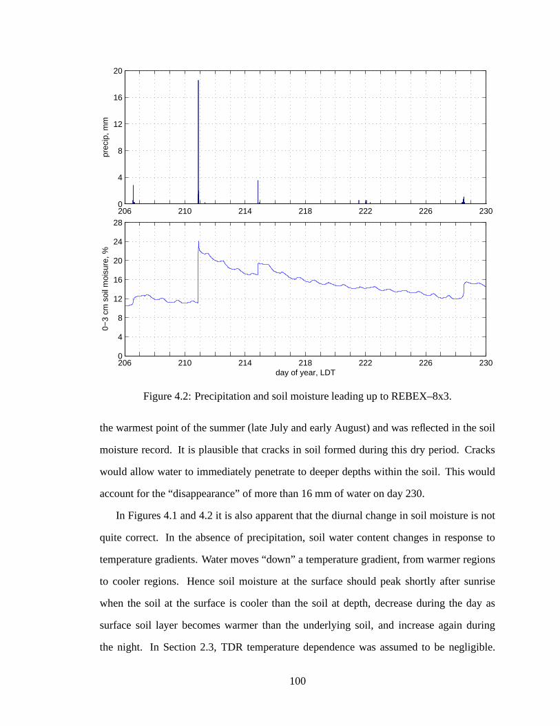
206 210 214 218 222 226 2300

4

8

12

16

20

prec

ip, m

m

206 210 214 218 222 226 2300

4

8

12

16

20

24

28

0−3

cm s

oil m

oisu

re, %

day of year, LDT

Figure 4.2: Precipitation and soil moisture leading up to REBEX–8x3.

the warmest point of the summer (late July and early August) and was reflected in the soil

moisture record. It is plausible that cracks in soil formed during this dry period. Cracks

would allow water to immediately penetrate to deeper depths within the soil. This would

account for the “disappearance” of more than 16 mm of water on day 230.

In Figures 4.1 and 4.2 it is also apparent that the diurnal change in soil moisture is not

quite correct. In the absence of precipitation, soil water content changes in response to

temperature gradients. Water moves “down” a temperature gradient, from warmer regions

to cooler regions. Hence soil moisture at the surface should peak shortly after sunrise

when the soil at the surface is cooler than the soil at depth, decrease during the day as

surface soil layer becomes warmer than the underlying soil, and increase again during

the night. In Section 2.3, TDR temperature dependence was assumed to be negligible.

100

229 230 231 232260

265

270

275

280

285

H−pol

brig

htne

ss te

mpe

ratu

re, K

observedmodel

229 230 231 232270

275

280

285

290

295

V−pol

brig

htne

ss te

mpe

ratu

re, K

day of year, LDT

observedmodel

Figure 4.3: Observed and modeled H– and V–pol brightness temperatures during REBEX–8x3.

From Figure 4.2, it appears that in fact the temperature dependence is slightly positive:

the increase in temperature during the day produces an apparent increase in the measured

water content. A soil model in combination with the calibration procedure described in

Section 2.3 could be used to find the true TDR temperature dependence for the soil at the

experiment site.

Figure 4.3 compares observed and modeled H– and V–pol brightness temperatures dur-

ing REBEX–8x3. The new zero–order model matches the observations closely. The model

correctly predicts the change in brightness as the soil and canopy warm and cool over the

course of the day. This performance is particularly striking considering the simplicity of

the model. The variable Tcanopy, defined as the average soil surface and vegetation IR ra-

101

diometric temperature, appears to capture the essential variation in vegetation temperature.

Temperature gradients within the canopy apparently have little affect on the microwave

brightness, although these gradients were not large during REBEX–8x3 (at most 4 K).

The radiometric sensitivity to Tcanopy can be found by taking the derivative of (3.2):

dTB dTcanopy

1 α

1 L 1 Rsoil L (4.2)

Recall that in the new model α and L, as well as Rsoil , are functions of θ and polarization.

Rsoil is also a function of soil moisture (and weakly of soil temperature). Using (4.2), the

sensitivity to canopy temperature can be found to vary only from about 0.64 to slightly less

than 0.66 K K 1 at H–pol for volumetric soil moisture ranging from 15 to 25% (the range

encountered during REBEX–8x3), and from about 0.63 to slightly more than 0.64 K K 1

at V–pol.

One strength of the model appears to be its sensitivity to canopy temperature. On the

other hand, there are three periods during which the model significantly deviates from the

observations. The first two periods occur during the night, on days 228/229 and 229/230.

After each of these two periods, the model “recovers” and predictions match observations

after about 10:00 in the morning. Could the presence of dew on the canopy, which would

have formed overnight and then evaporated after sunrise, have caused these errors? The

third period began late on day 230 and persisted until approximately 10:00 on day 231 at

V–pol, and throughout all of day 231 at H–pol. The start of this period coincides with

the first precipitation event which produced a change in 0–3 cm soil moisture of 9% and

certainly would have thoroughly wet the canopy.

Evidently, one model weakness is its incorrect representation of the effects of water

on the canopy. In all three periods, observed brightness is less than modeled brightness.

One hypothesis that can be formed from these observations is that water on the canopy ap-

pears to decrease the microwave brightness. This hypothesis will be tested in Sections 4.3

and 4.4. The decrease in brightness during the third period could also have been caused by

the change in soil moisture. To separate these effects, the sensitivity of microwave bright-

102

ness to changes in soil moisture in this particular field corn canopy must first be determined.

4.2 Soil Moisture Sensitivity

It is generally assumed that microwave brightness at 1.4 GHz is sensitive to soil mois-

ture up to a certain level of canopy biomass. This level has not been clearly defined. O’Neill

et al. [1996] reported a measurable sensitivity to soil moisture at a water column density

of 4 kg m 2. Ulaby et al. [1983] found that a change of one percent gravimetric soil mois-

ture produced a change in brightness temperature of 1 1 K for a water column density of

approximately 5 kg m 2. On the other hand, Brunfeldt and Ulaby [1984] observed no

difference between corn fields that either had metal screens placed at the soil surface, or

had no screens, at the middle of the growing season. Finally, Wang et al. [1984] observed

no sensitivity to soil moisture through a grass canopy with vegetation column density of

8 kg m 2. The point at which most vegetation canopies become opaque is believed by

many researchers to be at a water column density of about 5 kg m 2, but this must depend

upon the distribution of moisture in the canopy. For example, while Wang et al. [1984]

observed no sensitivity to soil moisture through a sufficiently dense grass canopy, a field

corn canopy of similar density but with water concentrated in stems and ears might be

sufficiently transparent to 1.4 GHz radiation to allow sensitivity to soil moisture.

The rain event on day 230 increased the 0–3 cm soil moisture by 9%. V–pol and H–pol

brightness reacted differently to this change in soil moisture. See Figure 4.4 for a closer

view of days 230 and 231. Immediately following the rain event there was a small in-

crease in the H–pol brightness temperature, from 262.0 K at 22:00 on day 230 to 263.5 K

at 6:00 on day 231. In this and the following analysis, several adjacent measurements of

brightness temperature have been averaged together in order to lower the uncertainty to

less than 0.2 K. This increase occurred while the 0–3 cm soil water content decreased by

1% as water infiltrated into the soil. On the other hand, the V–pol brightness tempera-

ture remained essentially constant during this same time period. This increase in H–pol

103

20:00 22:00 0:00 2:00 4:00 6:000

4

8

12REBEX−8x3

prec

ip, m

m20:00 22:00 0:00 2:00 4:00 6:00

12

14

16

18

20

22

24

26

vol s

oil m

oist

ure,

%

0 to 3 cm layer3 to 6 cm layer

20:00 22:00 0:00 2:00 4:00 6:00288

290

292

294

296

298

300te

mpe

ratu

re, K

IR vegetationIR soil1.5 cm soil

20:00 22:00 0:00 2:00 4:00 6:00260

265

270

275

280

285

290

brig

htne

ss te

mp,

K

day 230 and 231, LDT

V−polH−pol

Figure 4.4: Soil moisture at 0–3 cm and the difference between V–pol and H–pol brightnesstemperatures during REBEX–8x3.

brightness temperature was not consistent with changes in vegetation or soil temperatures

observed during the same period. Tcanopy and soil temperature at 1.5 cm both decreased

by 1.2 K and 1.4 K, respectively. It was also not likely to be caused by changes in water

intercepted by the canopy, which would be expected to remain constant during the night.

The change in H–pol brightness temperature appeared to be caused in large by the change

in soil moisture. The sensitivity at H–pol was approximately:

∆TB

∆VSM 1 5 K

1% 1 5 K %

1 (4.3)

This may be a conservative estimate, given the changes in soil and canopy temperatures

104

229 230 231 232220

230

240

250

260

270

280

290

brig

htne

ss te

mpe

ratu

re, K

day of year, LDT

V−pol Tsoil

(1 − Rsoil

)H−pol T

soil(1 − R

soil)

Figure 4.5: Modeled brightness temperature of the soil, just below the vegetation canopy,during REBEX–8x3.

which tended to decrease the brightness temperature during this time period. Taking into

account the competing effects of changes in soil and canopy temperatures, V–pol sensi-

tivity exists at this level of water column density, but it is much smaller ( 1K), perhaps

approximately equal to the sensitivity to canopy temperature.

The modeled brightness temperature of the soil, just below the vegetation canopy is

plotted in Figure 4.5. The change in soil moisture produces about a 23 K and 10 K change

at H– and V–pol, respectively. This sensitivity, about 2.6 K % 1 at H–pol, is consistent

with past research [Schmugge et al., 1986].

The 0–3 cm soil water content and the difference between V–pol and H–pol during

REBEX–8x3 is shown in Figure 4.6. If in fact there was a much higher sensitivity to

soil moisture at H–pol than at V–pol, there should be an obvious change in the difference

between the polarizations after the rain event. This is what was observed. Before the first

rain event, differences between V–pol and H–pol during the early morning hours (0:00 to

6:00) on days 229 and 230 were 7 to 8 K. After the rain event, H–pol was approximately

12 to 13 K lower than V–pol. During the rest of day 231, the difference between V–pol and

H–pol was larger than it was when the soil was drier on days 229 and 230.

105

229 230 231 23212

14

16

18

20

22

24

26

volu

met

ric s

oil m

oist

ure,

%

0 to 3 cm layer

229 230 231 2326

7

8

9

10

11

12

13

14

15

brig

htne

ss te

mpe

ratu

re, K

day of year (EDT), 2001

difference between V−pol and H−pol

Figure 4.6: Soil moisture at 0–3 cm and the difference between V–pol and H–pol brightnesstemperatures during REBEX–8x3.

4.3 Dew

Does dew on the canopy affect the brightness temperature? Theoretically, liquid water

on the scatterers in the canopy would increase their dielectric constant and loss. Higher

scatterer dielectric constant results in more scattering of radiation out of the beam. When

the scatterers have a higher loss, more of the scattered radiation is absorbed by other scat-

terers and hence less radiation can be scattered back into the beam. The result is an increase

in volume scattering and lower brightness temperatures. But this may be balanced or ex-

ceeded by an increase in emission due to an increase in the total water column density

[Ferrazzoli et al., 1992]. What is the net effect of water on the canopy?

A light dew was observed during data collection around 7:00 LDT on day 229. The dew

106

had evaporated by 10:00 that morning. The comparison of model predictions and observed

brightness temperatures in Figure 4.3 during this period suggest that the net effect of dew

is a decrease in the microwave brightness. No visits to the experiment site were made on

days 230 and 231, although the model predictions again indicate the likely presence of dew

during the night of days 229/230.

In order to determine the relative amount of dew during the night and early morning

hours of days 228/229 and 229/230, the canopy energy balance was evaluated to find the

latent heat transfer [Arya, 1988]:

HL Rn HS G ∆W (4.4)

Here HL is the flux of latent heat; Rn, the net radiation; HS, the sensible heat flux; G, the

ground heat flux; and ∆W , the rate of change of energy stored in the canopy. All of these

variables have the units of W m 2. The net radiation was not measured directly. It was cal-

culated using measurements of downwelling solar radiation, S, downwelling atmospheric

radiation, A, and vegetation IR radiometric temperature, Tveg:

Rn S A

aS σT 4veg (4.5)

where σ is the Stefan–Boltzmann constant and a is the albedo [Jacobs and Van Pul, 1990].

The vegetation radiometric temperature, instead of the canopy temperature, was used since

it is a direct measurement of the emission from the top of the canopy and a canopy emis-

sivity of unity at IR wavelengths has been assumed. The sensible heat flux was calculated

using bulk aerodynamic theory as follows:

HS ρair cp air CH

Tveg Tair u (4.6)

where ρair, is the density of air; cp air, air specific heat;

CH k2

ln

zu d

zom ψm

ζ 1

ln

za d

zoh ψh

ζ 1

(4.7)

the transfer coefficient; Tair, the air temperature measured at zair; u, the wind speed at zu;

k is Von Karman constant; d, the zero–plane displacement [Jacobs and Van Boxel, 1988];

107

zom, the roughness length for momentum [Jacobs and Van Boxel, 1988]; zoh, the roughness

length for heat; ψm and ψh are the profile diabatic correction factors for momentum and

heat, respectively; and ζ, the buoyancy parameter. lnzom

zoh 2 [Massman, 1999]. For

stable conditions typical at night, ψm ψh

6ln1 ζ [Yasuda, 1988] and ζ 0 4 [Wilson

et al., 1999]. Again, vegetation radiometric temperature, instead of canopy temperature,

was used since it is the top of the canopy that is exchanging heat with the atmosphere. The

rate of change of energy stored in the canopy was estimated using the canopy water column

density:

∆W Mw cp water ∆Tcanopy

∆t (4.8)

cp water is the specific heat of water; Tcanopy, the average of measured vegetation and soil

IR temperatures; and ∆Tcanopy, the change in Tcanopy during the measurement time interval

∆t. Ground heat flux was not measured, but estimated to be 15 W m 2 based upon

measurements made under a field corn canopy during REBEX–7 the previous summer.

Dew is the result of three processes [Monteith, 1957]. Dewfall, or water condensing

from air originating above the canopy, is by far the dominant process of dew formation in a

corn canopy when the soil surface is dry [Atzema et al., 1990]. Recall from (1.3) that latent

heat flux is equal to the rate of evaporation, transpiration, and condensation, E, multiplied

by the latent heat of vaporization, Le:

HL Le E (4.9)

At night, transpiration is negligible and a negative latent heat flux represents condensation

of water on the canopy. Figure 4.7 presents the canopy temperature, the cumulative amount

of condensation (dew) on the canopy since 18:00 LDT as predicted by (4.4), and the H–

and V–pol brightness temperatures for the night of days 228/229 and 229/230.

A negligible amount of dew on 229/230 is predicted by the energy balance model.

This is contrary to the predictions of the zero–order model in Figure 4.3. If the net effect

of dew is a decrease in brightness, smaller yet significant amount of dew should have

108

18:00 21:00 0:00 3:00 6:00286

288

290

292

294

296

cano

py te

mpe

ratu

re, K

LDT

228/229229/230

18:00 21:00 0:00 3:00 6:000

0.1

0.2

0.3

dew

, kg

m−

2

LDT

18:00 21:00 0:00 3:00 6:00266

268

270

272

274

276

brig

htne

ss te

mpe

ratu

re, K

H−pol

LDT

18:00 21:00 0:00 3:00 6:00274

276

278

280

282

284

brig

htne

ss te

mpe

ratu

re, K

LDT

V−pol

Figure 4.7: Canopy temperature, modeled dew deposition to the canopy, and H– and V–polbrightness temperatures during the night for days 228/229 and 229/230.

covered the vegetation on 229/230. Predictions of the zero–order model are depressed

by approximately 4 K at both H– and V–pol on day 228/229 and by approximately 2 to

2.5 K on 229/230. Although the energy balance method is physically correct, the theory

employed to compute the components of the energy balance are simplifications of complex

processes. The bulk aerodynamic transfer coefficient in (4.7) rests on many assumptions

and is suitable only for mean behavior. Furthermore, both changes in canopy energy storage

and ground heat flux were estimated. Even though ground heat flux was measured in a

similar situation, ground heat flux is difficult to measure [van Loon et al., 1998]. Errors

in any of the terms on the right–hand side of (4.4) would alter the amount of dew on the

canopy.

109

Although the total amount of dew predicted by the model in Figure 4.7 is reasonable,

it is probably incorrect. There is more confidence in the predictions of the relative amount

of dew deposited during the nights of 228/229 and 229/230. Uncertainty in the variables

of (4.4) are likely to be similar on consecutive nights. Taking the limitations of this mod-

eling approach into account, Figure 4.7 would at least indicate that less dew formed on the

canopy during the night of days 229/230 than on 228/229. If this is correct, then it appears

that: the net effect of dew is a decrease in brightness; and as more dew is deposited on the

canopy, the brightness continues to decrease.

From the zero–model comparison in Figure 4.3, it appears that the brightness tempera-

tures on the night of days 228/229 were progressively depressed as the dew formed, while

on the night of 229/230, dewfall occurred earlier, during a short period of time, and re-

mained on the canopy for the rest of the night. The gradual increase in the difference

between modeled and observed brightness on 228/229 in Figure 4.3 also supports the con-

clusions made earlier.

According to Figure 4.7, by the approximately 6:00 LDT on day 229, brightness tem-

peratures at both H– and V–pol were approximately 1 K lower than the brightness tem-

peratures recorded the next night, despite the fact that the canopy temperature at 6:00 on

day 229 was more than 1 K higher than on day 230. Soil moisture was virtually con-

stant during this time and soil temperature at 1.5 cm was 2 to 3 K less on the night of

229/230 (Figure 4.1). If there was in fact dew on the canopy on the night of 229/230, then

these observations again support the assertion that more dew the previous night resulted in

a larger decrease in the brightness temperature. It also appears that dew effects H– and

V–pol brightness equally.

The assertion that there was more dew on the canopy during the night of 228/229 than

229/230 is supported by measurements of air temperature, dew point temperature, and wind

speed in Figure 4.8. Dew point temperature was calculated from the air temperature and

relative humidity measured at 7.8 m. Wind speed was measured at 10 m. Note that at

110

18:00 21:00 0:00 3:00 6:00286

288

290

292

294

296

298

tem

pera

ture

, K

air temperature @ 7.8 mwind speed @ 10 mdew point temperature @ 7.8 m

18:00 21:00 0:00 3:00 6:000.0

1.5

3.0

4.5

6.0

7.5

9.0

win

d sp

eed,

m s

−1

days 228/229

LDT

18:00 21:00 0:00 3:00 6:00286

288

290

292

294

296

298

tem

pera

ture

, K

days 229/230

18:00 21:00 0:00 3:00 6:000.0

1.5

3.0

4.5

6.0

7.5

9.0

win

d sp

eed,

m s

−1

LDT

Figure 4.8: Air temperature at 7.8 m, wind speed at 10 m, and dew point temperature at7.8 m for the night of days 228/229 (top) and the night of days 229/230 (bottom).

18:00 the dew point temperature on 228/229 was much higher than on 229/230, indicating

that there was less moisture in the air above the canopy on the second night. On the night

of 228/229, the dew point temperature immediately began to decrease, suggesting either

condensation on the canopy was pulling moisture from the air, or the arrival of a drier air

mass. On the other hand, the dew point temperature on 229/230 remained roughly constant

the entire night. From 0:00 on, air and dew point temperatures were nearly identical on

both nights.

Another notable feature of Figure 4.8 is the difference in measured wind speed between

the two nights. The wind speed is considerably lower on 229/230. (The threshold of the

111

anemometer was 0 45 m s 1). According to bulk aerodynamic theory,

E ρair CWQ0 Q u (4.10)

where: CW is the transfer coefficient for water vapor, similar to the transfer coefficient for

heat in (4.7); Q0 is the mean specific humidity close to the surface; and Q is the mean

specific humidity at a reference height. During dew formation, Q0 Q (the surface is

drawing moisture from the air above) and E 0. Note that E is also directly proportional

to wind speed. Given the limitations of the bulk aerodynamic approach discussed earlier, a

higher wind speed on the night of 228/229 than on 229/230 would favor more dew. There

is a point at which a higher wind speed inhibits dew formation [Monteith, 1957], but the

wind on 228/229 was fairly gentle and likely below this level.

In summary, observations and modeling results support the hypothesis that water on the

canopy in the form of dew has the net effect of decreasing the microwave brightness. Fur-

thermore, it appears that as more water is deposited on the canopy, the microwave bright-

ness continues to decrease. Both polarizations appear to be affected equally.

4.4 Intercepted Precipitation

The data from REBEX–8x3 in Figure 4.1 and Figure 4.4 show that H–pol and V–pol

both experienced sharps drops during each rain event. On day 230, the H–pol brightness

temperature decreased by 13.4 K between 20:00 and 21:20 LDT, while V–pol decreased

by 10.8 K. During this same time period, the canopy temperature decreased by 4.1 K and

20 mm of precipitation fell, causing the 0–3 cm soil moisture to increase by 9%. Consid-

ering the analyses in Sections 4.2 and 4.3, the change in brightness on day 230 must be a

combination of changes in canopy temperature, soil moisture, and water on the canopy.

Given the sensitivity to soil moisture at H–pol in (4.3), a 9% change in soil moisture

would result in a 9% 1 5 K % 1 13 5 K change in brightness temperature. This is

slightly more than the entire change observed at H–pol. According to (4.2), the change in

112

canopy temperature during this period would result in a 4 1 K 0 6 K K 1 2 5 K change

in brightness temperature. If instead a soil moisture sensitivity of approximately 1 K % 1

is assumed, then a 13 4 2 5 9 2 K change could be attributed to the change in canopy

water. At V–pol, the soil moisture sensitivity is much less. The change in vegetation

temperature also accounts for 4 1 K 0 6 K K 1 2 5 K of the 10.8 K total change in

brightness temperature. The other 8.3 K must be a combination of enhanced scattering

due to the canopy water and to the change in soil moisture. If a soil moisture sensitivity

equivalent to the sensitivity to canopy temperature is assumed, then 9% 0 6 K % 1

5 4 K can be attributed to the change in soil moisture and the rest, 10 8 2 5 5 4 3 K

due to the effect of the intercepted precipitation. From these approximate calculations it

again appears that the net effect of intercepted precipitation is a decrease in brightness

temperature at both H– and V–pol. Volume scattering is enhanced more than emission.

The model comparison in Figure 4.3 supports a 2 to 3 K decrease in V–pol brightness

temperature due to the intercepted precipitation. By approximately 10:00 on day 231, the

model predictions again match the observations. These observations are consistent with a

drying of the canopy. On the other hand, modeled H–pol brightness remains higher than the

observed brightness throughout the course of day 231. Evidently, the canopy is more trans-

parent than predicted by the model: the soil moisture sensitivity predicted by the model is

too low. It also appears that dew can wet the canopy more than intercepted precipitation. A

maximum depression of about 4 K was observed during dew formation while the decrease

in brightness was slightly less (about 2 to 3 K) after the 21 mm precipitation event.

There were two other rain events during REBEX–8x3. Within less than 20 minutes

after the second rain event, both polarizations of microwave brightness recovered quickly

and started to increase. It was unlikely that such a quick change in brightness tempera-

ture was related to canopy water, despite the fact that the zero–order model V–pol pre-

dictions support the existence of a dry canopy after about 10:00 on day 231. Either the

microwave brightness was responding solely to changes in vegetation temperature, or per-

113

haps the canopy was still wet from the first rain event and water ponded between the rows

for a short period of time. Another sharp drop during the third rain event appears to be

caused by intercepted water. The model does not predict all of the drop observed at both

H– and V–pol and this drop remained through the end of the data record. It is not known

for certain whether the canopy dried during the 4 hours after the second rain event.

4.5 Conclusions

The new zero–order model, which considers κs to be a function of θ, correctly predicts

the change in brightness in response to changing vegetation temperature. In light of its

simplicity, this performance was not expected and its sensitivity to vegetation temperature

is the model’s main strength.

The net effect of water on a field corn canopy, either in the form of dew or intercepted

precipitation, is to decrease the brightness temperature. Volume scattering is enhanced

more than emission. This effect is seen at both polarizations, and each polarization appears

to be affected equally. As more water is deposited on the canopy the brightness at both po-

larizations continues to decrease. At some point a decrease in brightness with canopy water

would no longer occur since there is a limit to the amount of water that a canopy can hold.

Depressions of about 2 to 4 K were observed. Dew can decrease the brightness more than

a soaking rain. The new zero–order model did not correctly predict this decrease in bright-

ness. In fact, any increase in canopy water (water column density) increases the brightness

predicted by the zero–order model. These predictions are opposite of what was observed in

field corn. For other canopies, the balance between enhancement of volume scattering and

emission may depend on the vegetation type and observation frequency [Wigneron et al.,

1996] and water on the canopy may significantly bias soil moisture retrievals in either di-

rection.

Finally, a robust sensitivity to changes in soil moisture, approximately 1 to 1.5 K per

% 0–3 cm volumetric water content, was observed at H–pol in field corn at a water col-

114

0 2 4 6 80

1

2

3

4

water column density, kg m−2

|soi

l moi

stur

e se

nsiti

vity

|, K

%−

1

nonscattering canopynew zero−order modelSchmugge et al.O‘Neill et al.Chauhan et al.Ulaby et al.Hornbuckle et al.

Figure 4.9: Modeled and measured sensitivity of H–pol 1.4 GHz brightness temperature tovolumetric soil moisture in field corn.

umn density of 6.3 kg m 2, the highest column density observed during the summer.

The sensitivity at V–pol was less than 1 K and similar in magnitude to the sensitivity to

vegetation temperature. Soil moisture sensitivity as predicted for a nonscattering canopy

(τ b Mw b 0 115 [Jackson and O’Neill, 1990]), the new zero–order model, and the

sensitivities reported in field corn from aircraft platforms [Chauhan et al., 1994; O’Neill

et al., 1996; Ulaby et al., 1983], a bare soil sensitivity established by many field experi-

ments both from both airplane platforms and tower/truck–mounted radiometers [Schmugge

et al., 1986], and this dissertation for H–pol brightness temperature at 1.4 GHz is plot-

ted in Figure 4.9. The soil moisture sensitivity reported in this dissertation is significantly

higher than that predicted for an equivalent nonscattering canopy and by the new zero–order

model.

It can be concluded that both the amount of water in the canopy (water column density),

and its distribution play an important role in determining soil moisture sensitivity. Hence

canopies such as field corn in which the moisture is concentrated in stems and fruit appear

115

−6 −4 −2 0 2 4 6anticipated change in brightness temperature, K

1.4 GHz (λ = 21 cm), Mw = 6.3 kg m−2

soil moisture (4%)

canopy water (≈ 0.2 kg m−2)

vegetation temperature (10 K)

nonscattering canopyscattering canopy

Figure 4.10: Anticipated change in H–pol brightness temperature in response to typicalchanges in vegetation temperature, soil moisture, and canopy water at 1.4 GHz for a real(scattering) mature field corn canopy and an equivalent nonscattering canopy

.

more transparent than nonscattering canopies such as grass where the water is more evenly

spread over the entire canopy volume. The increased sensitivity to soil moisture could be

because the canopy is in fact more transparent than predicted, or because the zero–order

model does not account for reflections between the canopy and the soil surface. Enhanced

backscatter from scattering canopies has been observed in radar experiments. There may

be a similar effect in radiometry.

With an appropriate emission model that can account for both volume scattering and

the effects of water on the canopy, microwave radiometry will be able to detect changes

in soil moisture of less than 2%, given a typical microwave radiometer NE∆T of 1 K, at

all stages of field corn development (growth, maturity, and senescence). The zero–order

model is a strong candidate, if its two main weaknesses (sensitivity to canopy water and

H–pol transparency) can be rectified.

116

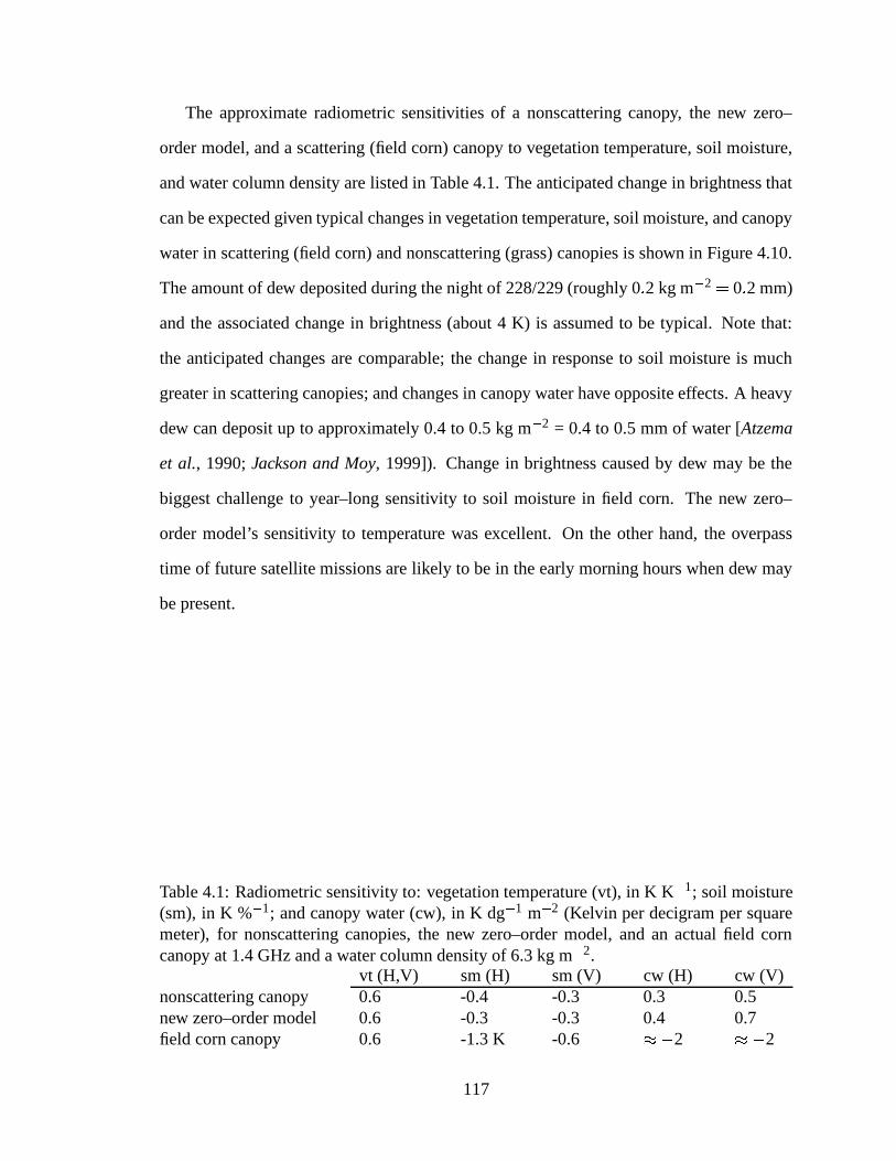
The approximate radiometric sensitivities of a nonscattering canopy, the new zero–

order model, and a scattering (field corn) canopy to vegetation temperature, soil moisture,

and water column density are listed in Table 4.1. The anticipated change in brightness that

can be expected given typical changes in vegetation temperature, soil moisture, and canopy

water in scattering (field corn) and nonscattering (grass) canopies is shown in Figure 4.10.

The amount of dew deposited during the night of 228/229 (roughly 0 2 kg m 2 0 2 mm)

and the associated change in brightness (about 4 K) is assumed to be typical. Note that:

the anticipated changes are comparable; the change in response to soil moisture is much

greater in scattering canopies; and changes in canopy water have opposite effects. A heavy

dew can deposit up to approximately 0.4 to 0.5 kg m 2 = 0.4 to 0.5 mm of water [Atzema

et al., 1990; Jackson and Moy, 1999]). Change in brightness caused by dew may be the

biggest challenge to year–long sensitivity to soil moisture in field corn. The new zero–

order model’s sensitivity to temperature was excellent. On the other hand, the overpass

time of future satellite missions are likely to be in the early morning hours when dew may

be present.

Table 4.1: Radiometric sensitivity to: vegetation temperature (vt), in K K 1; soil moisture

(sm), in K % 1; and canopy water (cw), in K dg

1 m 2 (Kelvin per decigram per square

meter), for nonscattering canopies, the new zero–order model, and an actual field corncanopy at 1.4 GHz and a water column density of 6.3 kg m

2.vt (H,V) sm (H) sm (V) cw (H) cw (V)

nonscattering canopy 0.6 -0.4 -0.3 0.3 0.5new zero–order model 0.6 -0.3 -0.3 0.4 0.7field corn canopy 0.6 -1.3 K -0.6 2 2

117

CHAPTER 5

Summary, Contributions, and Future Work

This final chapter includes a summary of the dissertation, identification of significant

contributions, and recommended future work.

5.1 Summary

Many of the impacts of climate change will be expressed in the water cycle. Microwave

radiometry is sensitive to the quantity and distribution of moisture in soil and vegetation.

Recent advances in radiometer technology and data assimilation techniques offer the pos-

sibility of real–time soil moisture measurements on a global scale. Critical to this vision

is the development of reliable models of land surface microwave brightness. In this dis-

sertation, measurements of 1.4 GHz brightness, micrometeorology, and soil moisture were

collected over the course of the growing season in a field of corn to determine how scatter-

ing canopies differ from the predictions made by models that are only strictly appropriate

for weakly–scattering canopies. Of greatest interest was how the amount and distribution

of moisture in vegetation influences microwave brightness.

5.2 Contributions

Both polarizations of the 1.4 GHz brightness of a field corn canopy are isotropic in

azimuth during most of the growing season. When the canopy is senescent, 1.4 GHz

118

brightness is a strong function of row direction. At H–pol, brightness is highest par-

allel to the rows, while at V–pol, brightness is highest perpendicular to the rows.

Brightness temperature changes by 5 to 10 K in azimuth, depending on the incidence

angle. These findings greatly simplify the formulation of appropriate models of land

surface brightness. Leaves were seen to play an important role: instead of acting sim-

ply as a “cloud” of moisture, they scatter microwave radiation and mask the internal,

stem–dominated structure of a field corn canopy. At senescence when they lose their

water, they become essentially invisible and the internal structure is exposed.

The question is raised whether other biophysical processes, associated with periods

of drought or extreme wetness, could cause changes in the effective canopy consti-

tutive properties. In many areas, agricultural fields are strictly planted N–S or E–W,

and azimuthal anisotropy at senescence will contribute to the inter–pixel variability

of satellite measurements. Errors of 5 to 10 K may translate into errors of 10 to 20%

in soil moisture estimation.

The zero–order radiative transfer model, used by many researchers because of its

simplicity, could not reproduce the observed change in brightness with incidence

angle measured in a field corn canopy. Validation of this model by other researchers

has occurred only at angles of incidence near nadir. The measurements reported in

this dissertation represent the first reported systematic investigation of the variation

with incidence angle. Significant scatter darkening was found. Without knowledge of

the behavior of scatter darkening, soil moisture retrievals would have a wet bias, on

the order of 2 to 12% at H–pol. These findings are timely since the first significant

1.4 GHz radiometer (SMOS) will be launched within the next few years. Initial

versions of algorithms constructed for this mission will utilize V–pol brightness at

large incidence angles to estimate biomass. Scatter darkening at V–pol was even

greater than at H–pol. If this effect were ignored, vegetation column density would

119

be underestimated, leading to over prediction of soil moisture.

A new zero–order model was formulated to account for the observed variation with

incidence angle. This was accomplished by allowing the volume scattering coeffi-

cient to be a function of incidence angle and polarization. The canopy medium is

anisotropic in elevation. Potentially this model will be of great use for the SMOS

mission. The small magnitude of the scattering coefficients allows the zero–order

model to retain its limited physical significance. Surprisingly, scattering was more

important at H–pol than V–pol, lending more information on the role of leaves.

The new zero–order model was compared with continuous measurements of mi-

crowave brightness made in a field of mature corn. The new model correctly predicts

change in brightness in response to vegetation temperature. The weakness of this

and any other zero–order model is its under prediction of the H–pol soil moisture

sensitivity in heterogeneous canopies where the moisture is concentrated in stems

and fruit, and its inability to respond correctly to changes in canopy water, either in

the form of intercepted precipitation or dew. Both the distribution and amount of

water in the canopy were found to be important.

Soil moisture sensitivity at H–pol was found to be at least 1 K % 1 in a mature field

corn canopy. This sensitivity is much higher than expected, both from model pre-

dictions and the results of previous research. With an appropriate emission model,

there will be significant soil moisture sensitivity throughout the growing season in

most, and perhaps all, agricultural crops. There are no other published records of

soil moisture sensitivity at such a high level of vegetation column density. Only the

use of a unique technique, consisting of simultaneous analyses of continuous mea-

surements of microwave brightness, micrometeorology, and soil moisture, allowed

this observation of sensitivity to be made.

An increase in canopy water, either in the form of intercepted precipitation or dew,

120

has the net effect of decreasing the microwave brightness in a corn canopy. This ef-

fect was observed at both polarizations, and each polarization appeared to be affected

equally. This is opposite to what had been assumed previously. This work also marks

the first time the effects of dew on the brightness have been successfully identified.

As more water is deposited on the canopy, the brightness at both polarizations con-

tinues to decrease. Depressions of 2 to 4 K were observed. Dew can decrease the

brightness more than a soaking rain.

The radiometric sensitivities to soil moisture, vegetation temperature, and canopy

water for nonscattering and scattering canopies were found at a vegetation column

density of 8 kg m 2. The expected change in brightness is comparable for typical

changes in these three variables. Accounting for the presence of dew and the corre-

sponding decrease in brightness may be the biggest challenge to year–long sensitivity

to soil moisture in agricultural crops.

Precise and continuous measurements of brightness temperature, micrometeorology,

and soil moisture were made on the plot scale. A unique measurement technique

allowed the calibration of buried soil moisture sensors, This rare data set can be used

in many more investigations.

5.3 Future Work

Hypothesis:

Models of microwave brightness can be improved by taking into account the

static and time–varying spatial distribution of water in and on the vegetation,

along with canopy geometry.

I propose to develop a detailed soil–vegetation–atmosphere transfer (SVAT) model to

couple with models of microwave emission in order to further improve brightness modeling

by taking into account temperature variations and the time–varying spatial distribution of

121

water in and on the vegetation. I plan to test these coupled models with data I have collected

during my thesis work and in future plot–scale field experiments. Ultimately, these models

will be used in conjunction with future satellite measurements to predict the moisture and

energy exchange between the land surface and the atmosphere on regional scales.

Coupled SVAT and microwave brightness models allow the integration of many types

of observations, both of microwave brightness and micrometeorology, over long periods of

time. Through this integration, subtle physical properties can be uncovered. The power of

this approach is illustrated in Chapters 3 and 4 of this dissertation. Without this time-series

of microwave brightness, micrometeorology, and soil moisture data, I would not have been

able to discover the relative influences of canopy anisotropy, vegetation temperature, soil

moisture, and canopy water. This concept of using other data besides simply the microwave

brightness over longer periods of time is much like using the context of a sentence to

decipher an unknown word, as opposed to only examining the word itself. I would not have

been able to draw these conclusions if only observations of microwave brightness had been

made, or if the observations had been too sparse (e.g. once daily measurements as typically

recorded in other investigations). I suspect much more information can be extracted from

this existing data set using coupled SVAT and microwave brightness models.

Although developing and validating a new SVAT model will be challenging, it may in

itself not be an entirely new research activity. It will, however, enable me to later pursue

original research on how time-varying spatial distributions of water in and on the vegetation

canopy can effect the microwave brightness and its sensitivity to soil moisture. Together,

the new coupled SVAT and microwave models would enable me to improve the fundamen-

tal physics of microwave scattering models and ultimately to confront other central scien-

tific issues, such as understanding the roles of land surface energy and water exchanges

and their correct scale of representation in models [National Research Council, 1999] in

anticipation of the first significant 1.4 GHz satellite radiometer, scheduled for launch in

2005 [Kerr et al., 2001]. My other future research goals include:

122

further development of in situ soil moisture measurement expertise with single fre-

quency (impedance probes) and multi–frequency (time domain reflectometry) instru-

ments;

development of new single frequency and multi–frequency instruments to measure

the time–varying distribution of water in vegetation;

development of SVAT / microwave brightness models for several types of vegetation;

determining the scales at which SVAT / microwave brightness models correctly an-

ticipate soil moisture, brightness, and surface fluxes;

extending point–scale (one-dimensional) SVAT / microwave brightness models to

two and three dimensions;

and incorporating SVAT / microwave brightness models into numerical weather pre-

diction models.

123

BIBLIOGRAPHY

124

BIBLIOGRAPHY

Anderson, J., H. van den Dool, A. Barnston, W. Chen, W. Stern, and J. Ploshay, Present–day capabilities of numerical and statistical models for atmospheric extratropical seasonalsimulation and prediction, Bull. Amer. Meteor. Soc., 80, 1349–1361, 1999.

Arya, S. P., Introduction to Micrometeorology, Academic Press, San Diego, CA, 1988.

Atzema, A. J., A. F. G. Jacobs, and L. Wartena, Moisture distribution within a maize cropdue to dew, Neth. J. of Agric. Sci., 38, 117–129, 1990.

Baker, J. M., and R. J. Lascano, The spatial sensitivity of time–domain reflectometry, SoilSci., 147, 378–384, 1989.

Beers, Y., Introduction to the Theory of Error, Addison–Wesley, Reading, MA, 1962.

Beljaars, A. C. M., and P. Viterbo, Soil moisture – precipitation interaction: Experiencewith two land surface schemes in the ECMWF model, in Global Energy and Water Cycles,edited by K. A. Browning and R. J. Gurney, Cambridge University Press, Cambridge, UK,1999.

Bohren, C. F., and D. R. Huffman, Absorption and Scattering of Light by Small Particles,John Wiley & Sons, Inc., New York, 1998.

Bonan, G. B., and L. M. Stillwell-Soller, Soil water and the persistence of floods anddroughts in the Mississippi River Basin, Water Resour. Res., 34, 2693–2701, 1998.

Brunfeldt, D. R., and F. T. Ulaby, Measured microwave emission and scattering in vege-tation canopies, IEEE Trans. Geosci. Remote Sens., GE–22, 520–524, 1984.

Brunfeldt, D. R., and F. T. Ulaby, Microwave emission from row crops, IEEE Trans.Geosci. Remote Sens., GE–24, 353–359, 1986.

Brutsaert, W., Evaporation in the Atmosphere: Theory, History, and Applications, D.Reidel, Boston, 1984.

Burke, E. J., L. A. Bastidas, and W. J. Shuttleworth, Exploring the potential for multi-patch soil–moisture retrievals using multiparameter optimization techniques, IEEE Trans.Geosci. Remote Sens., 40, 1114–1120, 2002.

Calvet, J.-C., and J. Noilhan, From near–surface to root–zone soil moisture using year–round data, J. Hydromet., 1, 393–411, 2000.

125

Calvet, J.-C., J. Noilhan, and P. Bessemoulin, Retrieving the root–zone soil moisture fromsurface soil moisture or temperature estimates: A feasibility study based on field mea-surements, J. Appl. Meteor., 37, 371–386, 1998.

Campbell, G. S., and J. M. Norman, An Introduction to Environmental Biophysics,Springer–Verlag, New York, 1998.

Campbell Scientific, Inc., CR10X Measurement and Control Module Operator’s Manual,Logan, UT, 2001.

Chang, J.-T., and P. J. Wetzel, Effects of spatial variations of soil moisture and vegetationon the evolution of a prestorm environment: A numerical case study, Mon. Weather Rev.,119, 1368–1390, 1991.

Chauhan, N. S., D. M. Le Vine, and R. H. Lang, Discrete scatter model for microwaveradar and radiometer response to corn: Comparison of theory and data, IEEE Trans.Geosci. Remote Sens., 32, 416–426, 1994.

Choudhury, B. J., T. J. Schmugge, A. Chang, and R. W. Newton, Effect of surface rough-ness on the microwave emission from soils, J. Geophys. Res., 84, 5699–5706, 1979.

Choudhury, B. J., T. J. Schmugge, and T. Mo, A parameterization of effective soil tem-perature for microwave emission, J. Geophys. Res., 87, 1301–1304, 1982.

Cole, K. S., and R. H. Cole, Dispersion and absorption in dielectrics. I. Alternating currentcharacteristics, J. Chem. Phys., 9, 341–351, 1952.

Crosson, W. L., C. A. Laymon, R. Inguva, and C. Bowman, Comparison of two microwaveradiobrightness models and validation with field measurements, IEEE Trans. Geosci. Re-mote Sens., 40, 143–152, 2002.

Curtis, J. O., Moisture effects on the dielectric properties of soils, IEEE Trans. Geosci.Remote Sens., 39, 125–128, 2001.

Dasberg, S., and J. W. Hopmans, Time domain reflectometry calibration for uniformly andnonuniformily wetted sandy and clayey loam soils, Soil Sci. Soc. Am. J., 56, 1341–1345,1992.

De Loor, G. P., Dielectric properties of heterogeneous mixtures, Ph.D. thesis, Universityof Leiden, Netherlands, 1956.

Debye, P. J. W., Polar Molecules, Dover, New York, 1929.

Delta–T Devices Ltd., Theta Probe Soil Moisture Sensor User Manual Type ML2x, Cam-bridge, England, 1999.

Delworth, T., and S. Manabe, The influence of soil wetness on near–surface atmosphericvariability, J. Climate, 2, 1447–1462, 1989.

126

Dirksen, C., and S. Dasberg, Improved calibration of time domain reflectometry soil watercontent measurements, Soil Sci. Soc. Am. J., 57, 660–667, 1993.

Dirmeyer, P. A., and K. L. Brubaker, Contrasting evaporative moisture sources during thedrought of 1988 and the flood of 1993, J. Geophys. Res., 104, 19,383–19,397, 1999.

Dirmeyer, P. A., F. J. Zeng, A. Ducharne, J. C. Morrill, and R. D. Koster, The sensitivityof surface fluxes to soil water content in three land surface schemes, J. Hydromet., 1,121–134, 2000.

Dobson, M. C., F. T. Ulaby, M. T. Hallikainen, and M. A. El-Rayes, Microwave dielectricbehavior of wet soil – part II: Dielectric mixing models, IEEE Trans. Geosci. RemoteSens., GE–23, 35–46, 1985.

Douglas, E. M., R. M. Vogel, and C. N. Kroll, Trends in floods and low flows in the UnitedStates: Impact of spatial correlation, J. Hydrol., 240, 90–105, 2000.

Dutton, E. G., J. J. Michalsky, T. Stoffel, B. W. Forgan, J. Hickey, D. W. Nelson, T. L.Alberta, and I. Reda, Measurement of broadband diffuse solar irradiance using currentcommercial instrumentation with a correction for thermal offset errors, J. Atmos. Ocean.Tech., 18, 297–314, 2001.

Eagleman, J. R., and W. C. Lin, Remote sensing of soil moisture by a 21–cm passiveradiometer, J. Geophys. Res., 81, 3660–3666, 1976.

Easterling, D. R., J. L. Evans, P. Y. Groisman, T. R. Karl, K. E. Kunkel, and P. Ambenje,Observed variability and trends in extreme climate events: A brief review, Bull. Amer.Meteor. Soc., 81, 417–425, 2000a.

Easterling, D. R., G. A. Meehl, C. Parmesan, S. A. Changnon, T. R. Karl, and L. O.Mearns, Climate extremes: Observations, modeling, and impacts, Science, 289, 2068–2074, 2000b.

Easterling, D. R., et al., Maximum and minimum temperature trends for the globe, Sci-ence, 277, 364–367, 1997.

Eltahir, E. A. B., A soil moisture – rainfall feedback mechanism 1. Theory and observa-tions, Water Resour. Res., 34, 765–776, 1998.

England, A. W., Thermal microwave emission from a scattering layer, J. Geophys. Res.,80, 4484–4496, 1975.

England, A. W., and G. R. Johnson, Microwave brightness spectra of layered media, Geo-physics, 42, 514–521, 1977.

Entekhabi, D., H. Nakamura, and E. G. Njoku, Solving the inverse problem for soilmoisture and temperature profiles by sequential assimilation of multifrequency remotelysensed observations, IEEE Trans. Geosci. Remote Sens., 32, 438–447, 1994.

127

Entekhabi, D., et al., An agenda for land surface hydrology research and a call for thesecond international hydrological decade, Bull. Amer. Meteor. Soc., 80, 2043–2058, 1999.

Fairall, C. W., P. O. G. Persson, E. F. Bradley, R. E. Payne, and S. P. Anderson, A newlook at calibration and use of Eppley Precision Infrared Radiometers. Part I: Theory andapplication, J. Atmos. Ocean. Tech., 15, 1229–1242, 1998.

Ferrazzoli, P., S. Paloscia, P. Pampaloni, G. Schiavon, D. Solimini, and P. Coppo, Sen-sitivity of microwave measurements to vegetation biomass and soil moisture content: Acase study, IEEE Trans. Geosci. Remote Sens., 30, 750–756, 1992.

Findell, K. L., Atmospheric controls on soil moisture – boundary layer interactions, Ph.D.thesis, Massachusettes Institute of Technology, 2001.

Findell, K. L., and E. A. B. Eltahir, An analysis of the soil moisture – rainfall feedback,based on direct observations from Illinois, Water Resour. Res., 33, 725–735, 1997.

Findell, K. L., and E. A. B. Eltahir, Analysis of the pathways relating soil moisture andsubsequent rainfall in Illinois, J. Geophys. Res., 104, 31,565–31,574, 1999.

Fischman, M. A., Development of a direct–sampling digital correlation radiometer forearth remote sensing applications, Ph.D. thesis, The University of Michigan, 2001.

Fischman, M. A., and A. W. England, Sensitivity of a 1.4 GHz direct–sampling radiome-ter, IEEE Trans. Geosci. Remote Sens., 37, 2172–2180, 1999.

Galantowicz, J. F., D. Entekhabi, and E. G. Njoku, Tests of sequential data assimilation forretrieving profile soil moisture and temperature from observed L–band radiobrightness,IEEE Trans. Geosci. Remote Sens., 37, 1860–1870, 1999.

Giorgi, F., L. O. Mearns, C. Shields, and L. Mayer, A regional model study of the im-portance of local versus remote controls of the 1988 drought and the 1993 flood over thecentral United States, J. Climate, 9, 1150–1168, 1996.

Grant, E., T. Buchanan, and T. Cook, Dielectric behavior of water at microwave frequen-cies, J. Chem. Phys., 26, 156–161, 1957.

Groisman, P. Y., R. W. Knight, and T. R. Karl, Heavy precipitation and high streamflowin the contiguous United States: Trends in the twentieth century, Bull. Amer. Meteor. Soc.,82, 219–246, 2001.

Groisman, P. Y., et al., Changes in the probability of heavy precipitation: Important indi-cators of climatic change, Climatic Change, 42, 243–283, 1999.

Hallikainen, M. T., F. T. Ulaby, M. C. Dobson, M. A. El-Rayes, and L.-K. Wu, Microwavedielectric behavior of wet soil – part I: Empirical models and experimental observations,IEEE Trans. Geosci. Remote Sens., GE–23, 25–34, 1985.

Hanks, R. J., Applied Soil Physics, Second Edition, Springer–Verlag, New York, 1992.

128

Hillhorst, M. A., C. Dirksen, F. W. H. Kampers, and R. A. Feddes, Dielectric relaxationof bound water versus soil matric pressure, Soil Sci. Soc. Am. J., 65, 311–314, 2001.

Hoekstra, P., and A. Delaney, Dielectric properties of soils at UHF and microwave fre-quencies, J. Geophys. Res., 79, 1699–1708, 1974.

Hoekstra, P., and W. Doyle, Dielectric relaxation of surface adsorbed water, J. ColloidInterface Sci., 36, 513, 1972.

Hoffert, M. I., et al., Advanced technology paths to global climate stability: Energy for agreenhouse planet, Science, 298, 981–987, 2002.

Hong, S.-Y., and E. Kalnay, Role of sea surface temperature and soil–moisture feedbackin the 1998 Oklahoma–Texas drought, Nature, 408, 842–844, 2000.

Hong, S.-Y., and H.-L. Pan, Impact of soil moisture anomalies on seasonal, summer-time circulation over North America in a regional climate model, J. Geophys. Res., 105,29,625–29,634, 2000.

Houser, P. R., W. J. Shuttleworth, J. S. Famiglietti, H. V. Gupta, K. H. Syed, and D. C.Goodrich, Integration of soil moisture remote sensing and hydrologic modeling using dataassimilation, Water Resour. Res., 34, 3405–3420, 1998.

Intergovernmental Panel on Climate Change, Climate Change 1995: The Science of Cli-mate Change, Cambridge University Press, London, 1996.

Jackson, T. J., Measuring surface soil moisture using passive microwave remote sensing,Hydrol. Processes, 7, 139–152, 1993.

Jackson, T. J., and L. Moy, Dew effects on passive microwave observations of land sur-faces, Remote Sens. Environ., 70, 129–137, 1999.

Jackson, T. J., and P. E. O’Neill, Attenuation of soil and microwave emission by corn andsoybeans at 1.4 and 5 GHz, IEEE Trans. Geosci. Remote Sens., 28, 978–980, 1990.

Jackson, T. J., T. J. Schmugge, and J. R. Wang, Passive microwave remote sensing of soilmoisture under vegetation canopies, Water Resour. Res., 18, 1137–1142, 1982.

Jackson, T. J., P. E. O’Neill, and C. T. Swift, Passive microwave observation of diurnalsurface soil moisture, IEEE Trans. Geosci. Remote Sens., 35, 1210–1222, 1997.

Jackson, T. J., T. J. Schmugge, P. E. O’Neill, and M. B. Parlange, Soil water infiltrationobservation with microwave radiometers, IEEE Trans. Geosci. Remote Sens., 36, 1376–1383, 1998.

Jacobs, A. F. G., and J. H. Van Boxel, Computational parameter estimation for a maizecrop, Bound. Lay. Meteorol., 42, 265–279, 1988.

Jacobs, A. F. G., and W. A. J. Van Pul, Seasonal changes in the albedo of a maize cropduring two seasons, Agric. For. Meteorol., 49, 351–360, 1990.

129

Karam, M. A., A physical model for microwave radiometry of vegetation, IEEE Trans.Geosci. Remote Sens., 35, 1045–1058, 1997.

Karl, T. R., and R. W. Knight, Secular trends of precipitation amount, frequency, andintensity in the United States, Bull. Amer. Meteor. Soc., 79, 1107–1119, 1998.

Karl, T. R., R. W. Knight, D. R. Easterling, and R. G. Quayle, Indices of climate changefor the united states, Bull. Amer. Meteor. Soc., 77, 279–291, 1996.

Kaspar, T. C., S. D. Logsdon, and M. A. Prieksat, Traffic pattern and tillage system effectson corn root and shoot growth, Agron. J., 87, 1046–1051, 1995.

Kerr, Y. H., P. Waldteufel, J.-P. Wigneron, J.-M. Martinuzzi, J. Font, and M. Berger, Soilmoisture retrieval from space: The soil moisture and ocean salinity (SMOS) mission,IEEE Trans. Geosci. Remote Sens., 39, 1729–1735, 2001.

Knight, J. H., Sensitivity of time domain reflectometry measurements to lateral variationsin soil water content, Water Resour. Res., 28, 2345–2352, 1992.

Knight, J. H., P. A. Ferre, D. L. Rudolph, and R. G. Kachanoski, A numerical analysis ofthe effects of coatings and gaps upon the relative dielectric permittivity measurement withtime domain reflectometry, Water Resour. Res., 33, 1455–1460, 1997.

Koster, R. D., and M. J. Suarez, The influence of land surface moisture retention on pre-cipitation statistics, J. Climate, 9, 2551–2567, 1996.

Koster, R. D., M. J. Suarez, and M. Heiser, Variance and predictability of precipitation atseasonal–to–interannual timescales, J. Hydromet., 1, 26–46, 2000.

Kunkel, K. E., K. Andsager, and D. R. Easterling, Long–term trends in extreme precipi-tation events over the conterminous United States, J. Climate, 12, 2515–2527, 1999a.

Kunkel, K. E., R. A. Pielke Jr., and S. A. Changnon, Temporal fluctuations in weather andclimate extremes that cause economic and human health impacts: A review, Bull. Amer.Meteor. Soc., 80, 1077–1098, 1999b.

Le Vine, D. M., Synthetic aperture radiometer systems, IEEE Trans. Micro. Theory Tech.,47, 2228–2236, 1999.

Le Vine, D. M., A. Griffis, C. T. Swift, and T. J. Jackson, ESTAR: A synthetic aperturemicrowave radiometer for remote sensing applications, Proc. IEEE, 82, 1787–1801, 1994.

Lee, J. K., and J. A. Kong, Passive microwave remote sensing of an anisotropic random–medium layer, IEEE Trans. Geosci. Remote Sens., GE–23, 924–932, 1985.

Lins, H. F., and J. R. Slack, Streamflow trends in the United States, Geophys. Res. Lett.,26, 227–230, 1999.

130

Liou, Y.-A., J. F. Galantowicz, and A. W. England, A land surface process / radiobright-ness model with coupled heat and moisture transport for prairie grassland, IEEE Trans.Geosci. Remote Sens., 37, 1848–1859, 1999.

Macelloni, G., P. Pampaloni, S. Paloscia, and R. Ruisi, Effects of spatial inhomogeneitiesand microwave emission enhancement in random media: An experimental study, IEEETrans. Geosci. Remote Sens., 34, 1084–1089, 1996.

Mahfouf, J.-F., Analysis of soil moisture from near–surface parameters: A feasibilitystudy, J. Appl. Meteor., 30, 1534–1547, 1991.

Manabe, S., Climate and the ocean circulation: 1, The atmospheric circulation and thehydrology of the earth’s surface, Mon. Weather Rev., 97, 739–805, 1969.

Massman, W. J., A model study of kB 1H for vegetated surfaces using ‘localized near–field’

Lagrangian theory, J. Hydrol., 223, 27–43, 1999.

Meehl, G. A., et al., An introduction to trends in extreme weather and climate events: Ob-servations, socioeconomic impacts, terrestrial ecological impacts, and model projections,Bull. Amer. Meteor. Soc., 81, 413–416, 2000.

Mintz, Y., and G. Walker, Global fields of soil moisture and land surface evapotranspira-tion derived from observed precipitation and surface air temperature, J. Appl. Meteor., 32,1305–1334, 1993.

Mo, T., B. J. Choudhury, T. J. Schmugge, J. R. Wang, and T. J. Jackson, A model for mi-crowave emission from vegetation–covered fields, J. Geophys. Res., 87, 11,229–11,237,1982.

Monteith, J. L., Dew, Quart. J. Roy. Meteorol. Soc., 83, 322–341, 1957.

National Research Council, Global Environmental Change: Research Pathways for theNext Decade, National Academy Press, Washington, DC, 1999.

Neild, R. E., D. A. Wilhite, and K. G. Hubbard, Preseason precipitation probabilities asan aid to corn planting decisions, Agric. For. Meteorol., 41, 259–266, 1987.

News and Notes, Record cold grips much of the nation in november and december: Two–month period is the coldest on record in the united states, Bull. Amer. Meteor. Soc., 82,499–500, 2001.

Newton, R. W., Microwave remote sensing and its application to soil moisture detection,Tech. Rep. Technical Report RSC–81, Texas A&M University, College Station, TX, 1977.

Newton, R. W., and J. W. Rouse, Jr., Microwave radiometer measurements of soil moisturecontent, IEEE Trans. Antennas Propagat., AP-28, 680–686, 1980.

Njoku, E., and J. A. Kong, Theory for passive microwave remote sensing of near–surfacesoil moisture, J. Geophys. Res., 82, 3108–3118, 1977.

131

Norman, J. M., and F. Becker, Terminology in thermal infrared remote sensing of naturalsurfaces, Agric. For. Meteorol., 77, 153–166, 1995.

Oglesby, R. J., and D. J. Erickson, Soil moisture and the persistence of North Americandrought, J. Climate, 2, 1362–1380, 1989.

Oh, Y., and Y. C. Kay, Condition for precise measurement of soil surface roughness, IEEETrans. Geosci. Remote Sens., 36, 691–695, 1998.

Oki, T., The global water cycle, in Global Energy and Water Cycles, edited by K. A.Browning and R. J. Gurney, Cambridge University Press, Cambridge, UK, 1999.

Olhoeft, G. R., Electrical properties of rocks, in Physical Properties of Rocks and Min-erals, edited by Y. S. Touloukian, W. R. Judd, and R. F. Roy, CINDAS Data Series onMaterial Properties, Hemisphere, New York, 1989.

O’Neill, P. E., T. J. Jackson, B. J. Blanchard, J. R. Wang, and W. I. Gould, Effects of cornstalk orientation and water content on passive microwave remote sensing of soil moisture,Remote Sens. Environ., 16, 55–67, 1984.

O’Neill, P. E., N. S. Chauhan, and T. J. Jackson, Use of active and passive microwaveremote sensing for soil moisture estimation through corn, Intl. J. Remote Sens., 17, 1851–1865, 1996.

Or, D., and J. M. Wraith, Temperature effects on soil bulk dielectric permittivity measuredby time domain reflectometry: A physical model, Water Resour. Res., 35, 371–383, 1999.

Pan, Z., M. Segal, R. Turner, and E. Takle, Model simulation of impacts of transientsurface wetness on summer rainfall in the United States Midwest during drought andflood years, Mon. Weather Rev., 123, 1575–1581, 1995.

Pepin, S., N. J. Livingston, and W. R. Hook, Temperature–dependent measurement errorsin time domain reflectometry determinations of soil water, Soil Sci. Soc. Am. J., 59, 38–43,1995.

Persson, M., and R. Berndtsson, Texture and electrical conductivity effects on temperaturedependency in time domain reflectometry, Soil Sci. Soc. Am. J., 62, 887–893, 1998.

Pitman, A. J., et al., Key results and implications from phase 1(c) of the Project for Inter-comparison of Land–surface Parameterization Schemes, Climate Dynamics, 15, 673–684,1999.

Pollack, H. N., S. Huang, and P.-Y. Shen, Climate change record in subsurface tempera-tures: A global perspective, Science, 282, 279–281, 1998.

Reda, I., J. R. Hickey, T. Stoffel, and D. Myers, Pyrgeometer calibration at the NationalRenewable Energy Laboratory (NREL), J. Atmos. Solar–Terr. Phys., 64, 1623–1629,2002.

132

Reichle, R. H., D. B. McLaughlin, and D. Entekhabi, Variational data assimilation ofmicrowave radiobrightness observations for land surface hydrology applications, IEEETrans. Geosci. Remote Sens., 39, 1708–1718, 2001.

Rhoades, J. D., N. A. Manteghi, P. J. Shouse, and W. J. Alves, Soil electrical conductivityand soil salinity: New formulations and calibrations, Soil Sci. Soc. Am. J., 53, 433–439,1989.

Rind, D., The influence of ground moisture conditions in North America on summer cli-mate as modeled in the GISS GCM, Mon. Weather Rev., 110, 1487–1494, 1982.

Roads, J., and A. Betts, NCEP–NCAR and ECMWF reanalysis surface water and energybudgets for the Mississippi River Basin, J. Hydromet., 1, 88–94, 2000.

Schmugge, T. J., Remote sensing of surface soil moisture, J. Appl. Meteor., 17, 1549–1557, 1978.

Schmugge, T. J., and B. J. Choudhury, A comparison of radiative transfer models forpredicting the microwave emission from soils, Radio Sci., 16, 927–938, 1981.

Schmugge, T. J., and T. J. Jackson, A dielectric model of the vegetation effects on themicrowave emission from soils, IEEE Trans. Geosci. Remote Sens., 30, 757–760, 1992.

Schmugge, T. J., P. Gloersen, T. Wilheit, and F. Geiger, Remote sensing of soil moisturewith microwave radiometers, J. Geophys. Res., 79, 317–323, 1974.

Schmugge, T. J., P. E. O’Neill, and J. R. Wang, Passive microwave soil moisture research,IEEE Trans. Geosci. Remote Sens., GE–24, 12–22, 1986.

Schulz, J.-P., L. Dumenil, J. Polcher, C. A. Schlosser, and Y. Xue, Land surface energyand moisture fluxes: Comparing three models, J. Appl. Meteor., 37, 288–307, 1998.

Segal, M., and R. W. Arritt, Nonclassical mesoscale circulations caused by surface sensi-ble heat–flux gradients, Bull. Amer. Meteor. Soc., 73, 1593–1604, 1992.

Seyfried, M. S., and M. D. Murdock, Response of a new soil water sensor to variable soil,water content, and temperature, Soil Sci. Soc. Am. J., 65, 28–34, 2001.

Sharratt, B. S., J. Zandlo, and G. Spoden, Frequency of precipitation across the northernU.S. corn belt, J. Appl. Meteor., 40, 183–191, 2001.

Shukla, J., and Y. Mintz, Influence of land–surface evapotranspiration on the earth’s cli-mate, Science, 215, 1498–1501, 1982.

Stogryn, A., Equations for calculating the dielectric constant of saline water, IEEE Trans.Micro. Theory Tech., MIT-19, 733–736, 1971.

Swift, C. T., D. M. Le Vine, and C. S. Ruf, Aperture synthesis concepts in microwaveremote sensing of the earth, IEEE Trans. Micro. Theory Tech., 39, 1931–1935, 1991.

133

Topp, G. C., J. L. Davis, and A. P. Annan, Electromagnetic determination of soil watercontent: Measurements in coaxial transmission lines, Water Resour. Res., 16, 574–582,1980.

Trenberth, K. E., and C. J. Guillemot, Physical processes involved in the 1988 droughtand 1993 floods in North America, J. Climate, 9, 1288–1298, 1996.

Ulaby, F. T., R. K. Moore, and A. K. Fung, Microwave Remote Sensing: Active andPassive, vol. 1-3, Artech House, Norwood, MA, 1981-1986.

Ulaby, F. T., M. Razani, and M. C. Dobson, Effects of vegetation cover on the microwaveradiometric sensitivity to soil moisture, IEEE Trans. Geosci. Remote Sens., GE–21, 51–61, 1983.

Ulaby, F. T., A. Tavakoli, and T. B. A. Senior, Microwave propagation constant for avegetation canopy with vertical stalks, IEEE Trans. Geosci. Remote Sens., GE–25, 714–725, 1987.

Vachaud, G., A. Passerat De Silane, P. Balabanis, and M. Vauclin, Temporal stability ofspatially measured soil water probability density function, Soil Sci. Soc. Am. J., 49, 822–827, 1985.

van Loon, W. K. P., H. M. H. Bastings, and E. J. Moors, Calibration of soil heat fluxsensors, Agric. For. Meteorol., 92, 1–8, 1998.

Walker, J., and P. R. Rowntree, The effect of soil moisture on circulation and rainfall in atropical model, Quart. J. Roy. Meteorol. Soc., 103, 29–46, 1977.

Wang, J. R., The dielectric properties of soil–water mixtures at microwave frequencies,Radio Sci., 15, 977–985, 1980.

Wang, J. R., R. W. Newton, and J. W. Rouse, Jr., Passive microwave remote sensing of soilmoisture: The effect of tilled row structure, IEEE Trans. Geosci. Remote Sens., GE–18,296–302, 1980a.

Wang, J. R., J. C. Shiue, and J. E. McMurtrey, III, Microwave remote sensing of soilmoisture content over bare and vegetated fields, Geophys. Res. Lett., 7, 801–804, 1980b.

Wang, J. R., J. C. Shiue, S. L. Chuang, R. T. Shin, and M. Dombrowski, Thermal mi-crowave emission from vegetated fields: A comparison between theory and experiment,IEEE Trans. Geosci. Remote Sens., GE–22, 143–150, 1984.

Washington, W. M., Climate–model responses to increased CO2 and other greenhousegases, in Climate System Modeling, edited by K. E. Trenberth, Cambridge UniversityPress, London, 1992.

Wetherald, R. T., and S. Manabe, Simulation of hydrologic changes associated with globalwarming, J. Geophys. Res., 107, 4379, doi:10.1029/2001JD001195, 2002.

134

Whalley, W. R., Considerations on the use of time–domain relflectometry (TDR) for mea-suring soil water content, J. Soil Sci., 44, 1–9, 1993.

White, I., J. H. Knight, S. J. Zegelin, and G. C. Topp, Comments on ’Considerations onthe use of time–domain relflectometry (TDR) for measuring soil water content’ by W. R.Whalley, Europ. J. Soil Sci., 45, 503–508, 1994.

Wigneron, J.-P., J.-C. Calvet, Y. Kerr, A. Chanzy, and A. Lopes, Microwave emissionof vegetation: Sensitivity to leaf characteristics, IEEE Trans. Geosci. Remote Sens., 31,716–726, 1993.

Wigneron, J.-P., J.-C. Calvet, and Y. Kerr, Monitoring water interception by crop fieldsfrom passive microwave observations, Agric. For. Meteorol., 80, 177–194, 1996.

Wigneron, J.-P., A. Olioso, J.-C. Calvet, and P. Bertuzzi, Estimating root zone soil mois-ture from surface soil moisture data and soil–vegetation–atmosphere transfer modeling,Water Resour. Res., 35, 3735–3745, 1999.

Wigneron, J.-P., L. Laguerre, and Y. H. Kerr, A simple parameterization of the L–bandmicrowave emission from rough agricultural soils, IEEE Trans. Geosci. Remote Sens., 39,1697–1707, 2001.

Wilson, T. B., W. L. Bland, and J. M. Norman, Measurement and simulation of dewaccumulation and drying in a potato canopy, Agric. For. Meteorol., 93, 111–119, 1999.

Wraith, J. M., and D. Or, Temperature effects on soil bulk dielectric permittivity measuredby time domain reflectometry: Experimental evidence and hypothesis development, WaterResour. Res., 35, 361–369, 1999.

Yasuda, N., Turbulent diffusivity and diurnal variations in the atmospheric boundary layer,Bound. Lay. Meteorol., 43, 209–221, 1988.

Yeh, T. C., R. T. Wetherald, and S. Manabe, The effect of soil moisture on the short–term climate and hydrology change: A numerical experiment, Mon. Weather Rev., 112,474–490, 1984.

135