Radiometric Quality of the MODIS Bands at 667 and 678nm

Gerhard Meistera, Bryan A. Franza

aNASA, Ocean Biology Processing Group, Code 614.2, Goddard Space Flight Center,

Greenbelt, MD 20771, USA;

ABSTRACT

The MODIS instruments on Terra and Aqua were designed to allow the measurement of chlorophyll fluorescenceeffects over ocean. The retrieval algorithm is based on the difference between the water-leaving radiances at667nm and 678nm. The water-leaving radiances at these wavelengths are usually very low relative to the top-of-atmosphere radiances. The high radiometric accuracy needed to retrieve the small fluorescence signal lead toa dual gain design for the 667 and 678nm bands. This paper discusses the benefits obtained from this designchoice and provides justification for the use of only one set of gains for global processing of ocean color products.Noise characteristics of the two bands and their related products are compared to other products of bands from412nm to 2130nm. The impact of polarization on the two bands is discussed. In addition, the impact of straylight on the two bands is compared to other MODIS bands.

Keywords: remote sensing, scanners, on-orbit calibration

1. INTRODUCTION

Two units of the Moderate-Resolution Imaging Spectroradiometer (MODIS)1 are currently in operation, provid-ing global coverage of top-of-atmosphere (TOA) radiances from 412nm to 14200nm. The first unit was launchedin December 1999 on NASA’s Earth Observing System (EOS) Terra satellite, the second on the Aqua satellitein May 2002. MODIS has 36 spectral bands on four different focal planes. The Ocean Biology Processing Group(OBPG) at NASA uses bands 8-16 with center wavelengths from 412nm to 869nm to produce the standard oceancolor data products.2 The basic ocean color products are water-leaving radiances from bands 8-14, see table 1.Bands 15 and 16 (748nm and 869nm) are used in the atmospheric correction process. All ocean color productsare derived from the water-leaving radiances. Recently, the OBPG included ocean color products from bands 1,3, and 4. More information on the ocean color products provided by the OBPG can be found at their website:http:oceancolor.gsfc.nasa.gov.

MODIS bands 8-12 and 15-16 each have 10 independent detectors, aligned in the along-track direction.MODIS is a scanning radiometer with a two-sided primary mirror, so every scan line consists of 10 lines in thealong-track direction (one for each detector) for a certain mirror side (adjacent scan lines are from alternatingmirror sides). The detectors of each band are shielded by a spectral filter that only transmits light in a certainwavelength range (e.g. from 662nm to 672nm for band 13; from 673nm to 683nm for band 14).

MODIS was the first instrument capable of measuring chlorophyll fluorescence from low earth orbits.3 Bands13 and 14 are very close spectrally, but band 14 is within the spectral region influenced by chlorophyll fluores-cence.4 The fluorescence line height (FLH) product is calculated based on the difference in the water-leavingradiances of these two bands. Noise limitations were an important consideration in the design of these twobands, because the difference of the water-leaving radiances of these two bands is very small compared to thetop-of-atmosphere (TOA) radiance (usually much less than 1%).

Further author information:G.M.: E-mail: Gerhard.Meister@nasa.gov

Table 1. MODIS ocean color bands and their center wavelengths λ. Band 6 is not listed here because 8 of its 10 detectorsare defunct on MODIS Aqua.

Band number 1 2 3 4 5 7 8 9 10 11 12 13 14 15 16λ[nm] 645 869 469 555 1240 2135 412 443 488 531 547 667 678 748 869

https://ntrs.nasa.gov/search.jsp?R=20110015306 2020-03-26T01:36:35+00:00Z

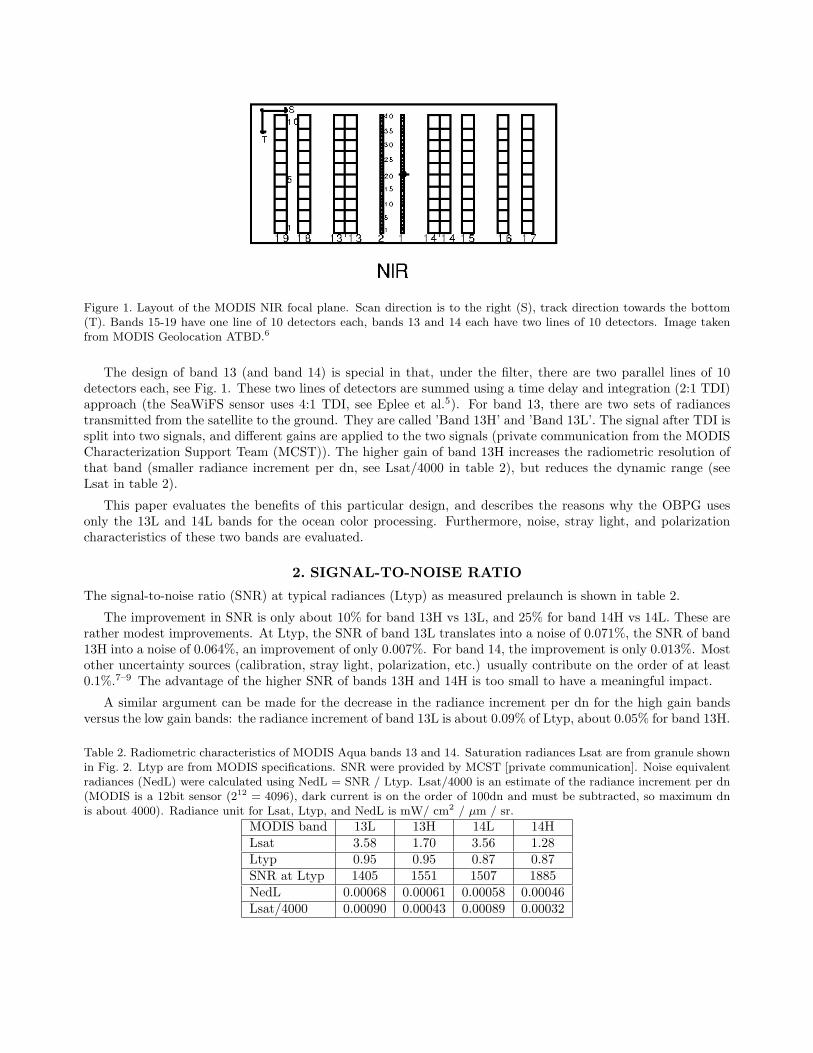
Figure 1. Layout of the MODIS NIR focal plane. Scan direction is to the right (S), track direction towards the bottom(T). Bands 15-19 have one line of 10 detectors each, bands 13 and 14 each have two lines of 10 detectors. Image takenfrom MODIS Geolocation ATBD.6

The design of band 13 (and band 14) is special in that, under the filter, there are two parallel lines of 10detectors each, see Fig. 1. These two lines of detectors are summed using a time delay and integration (2:1 TDI)approach (the SeaWiFS sensor uses 4:1 TDI, see Eplee et al.5). For band 13, there are two sets of radiancestransmitted from the satellite to the ground. They are called ’Band 13H’ and ’Band 13L’. The signal after TDI issplit into two signals, and different gains are applied to the two signals (private communication from the MODISCharacterization Support Team (MCST)). The higher gain of band 13H increases the radiometric resolution ofthat band (smaller radiance increment per dn, see Lsat/4000 in table 2), but reduces the dynamic range (seeLsat in table 2).

This paper evaluates the benefits of this particular design, and describes the reasons why the OBPG usesonly the 13L and 14L bands for the ocean color processing. Furthermore, noise, stray light, and polarizationcharacteristics of these two bands are evaluated.

2. SIGNAL-TO-NOISE RATIO

The signal-to-noise ratio (SNR) at typical radiances (Ltyp) as measured prelaunch is shown in table 2.

The improvement in SNR is only about 10% for band 13H vs 13L, and 25% for band 14H vs 14L. These arerather modest improvements. At Ltyp, the SNR of band 13L translates into a noise of 0.071%, the SNR of band13H into a noise of 0.064%, an improvement of only 0.007%. For band 14, the improvement is only 0.013%. Mostother uncertainty sources (calibration, stray light, polarization, etc.) usually contribute on the order of at least0.1%.7–9 The advantage of the higher SNR of bands 13H and 14H is too small to have a meaningful impact.

A similar argument can be made for the decrease in the radiance increment per dn for the high gain bandsversus the low gain bands: the radiance increment of band 13L is about 0.09% of Ltyp, about 0.05% for band 13H.

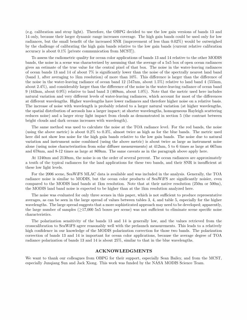
Table 2. Radiometric characteristics of MODIS Aqua bands 13 and 14. Saturation radiances Lsat are from granule shownin Fig. 2. Ltyp are from MODIS specifications. SNR were provided by MCST [private communication]. Noise equivalentradiances (NedL) were calculated using NedL = SNR / Ltyp. Lsat/4000 is an estimate of the radiance increment per dn(MODIS is a 12bit sensor (212 = 4096), dark current is on the order of 100dn and must be subtracted, so maximum dnis about 4000). Radiance unit for Lsat, Ltyp, and NedL is mW/ cm2 / µm / sr.

MODIS band 13L 13H 14L 14HLsat 3.58 1.70 3.56 1.28Ltyp 0.95 0.95 0.87 0.87SNR at Ltyp 1405 1551 1507 1885NedL 0.00068 0.00061 0.00058 0.00046Lsat/4000 0.00090 0.00043 0.00089 0.00032

Figure 2. Left: True color image of the test granule used in section 3. Image provided by LAADS web. Right: Locationof the granule on the globe. Image provided by OBPG.

Figure 3. Left: ratio of the low gain to the high gain L1B radiances for band 13. Right: same for band 14.

This corresponds to an improvement of 0.04%. For band 14, the improvement is 0.07%. These improvementsare small compared to most other uncertainty sources.

The radiance increments per dn decrease by more than 50% for the high gain bands relative to the low gainbands. These differences are much larger than the change in SNR, which implies that noise of the low gain bandsis not dominated by quantization noise.

3. ANALYSIS OF IMAGE DATA

MODIS Aqua granule A20072732135 (see Fig.2) was used to investigate the benefits of substituting bands 13Hand 14H for bands 13L and 14L.

From this granule, only pixels were selected where the flags ATMFAIL, LAND, STRAYLIGHT, CLDICE,CHLFAIL, MODGLINT were not set, and also where band 14H did not saturate (a saturation threshold of 1.25mW/ cm2 / µm / sr was chosen for band 14H, 14H always saturated when 13H saturated). The ratio of the lowgain to the high gain L1B radiances for the selected pixels are shown in Fig.3 as a function of low gain radiance,for each band 13 and 14.

It can be seen that there is some variation in the ratio of about ± 0.2%, and a bias of about 0.2%, withlow-gain bands higher than the high-gain bands.

Figure 4. Left: Measured ratio of 14L/13L over 14H/13H as a function of 14L/13L. Right: Simulated ratio of 14L/13Lover 14H/13H as a function of 14L/13L. Distribution of values along x-axis (14L/13L) is taken from the plot on the right,noise was added to ratio of 14L/13L over 14H/13H (setting 14H/13H equal to 14L/13L before noise was added), usingSNR from table 2.

Presumably, if the high gain bands were to be used instead of the low gain bands, they would be used in bothbands 13 and 14. The FLH algorithm depends on the difference of the radiance between the two bands. Fig.4shows the ratio of 14L/13L over 14H/13H as a function of 14L/13L.

It can be seen that there is almost no bias in the measured ratios (the mean of 14L/13L over 14H/13H is1.0002), but there is a noticeable variation (standard deviation is 0.0011). In order to test whether this variationcan be explained by the SNR obtained with the prelaunch SNR, we simulated this ratio, assuming the SNR atLtyp for all radiance levels (this assumption underestimates the noise, because most radiances where 14H doesnot saturate are below Ltyp). The results are shown in Fig. 4 as well.

The simulated ratios are very similar to the measured ratios. The simulated ratios have a slightly largerspread (standard deviation of all points is 0.0013). One possible explanation is that the noise in the measuredhigh gain band radiances is correlated with the noise in the low gain band radiances (there is no correlation inthe simulated radiances). Considering that for each band, both the high gain and the low gain radiances areextracted from the same data source (the sum of the two TDI detectors of each band), a certain amount ofcorrelation in the ratios 14L/13L over 14H/13H should be expected.

Fig.5 shows the FLH values from a subscene of the granule of Fig.2 (from the center of the granule, the USwest coast is part of the subscene) processed using SeaDAS 5.1.3 with the high gain bands (left) versus the lowgain bands (right). SeaDAS usually calculates the nLw of bands 13 and 14 using the low gain bands. To createthe nLw using the high gain bands for these plots, the low gain bands in the L1B file were overwritten with thehigh gain bands, after adjusting the mean L1B radiance of the high gain bands to the mean L1B radiance of thelow gain bands.

The images look very similar, with no apparent difference in the noise characteristics between the high gainand low gain image. The high gain image has stronger striping. For the low gain bands, the OBPG uses acorrection based on TOA residuals.10 This correction has not been calculated for the high gain bands, insteadthe low gain correction was applied. It is possible that the striping would be similar in both images if correctionsderived for the high gain bands were applied, although the corrections for high and low gain are expected to bevery similar.

Note that the low-gain bands provide more spatial coverage than the high-gain bands (black areas are largerin the plot on the left in Fig.5 than in the right plot, especially in the coastal area with high FLH values (red);San Francisco Bay (at 37◦ latitude and 122◦ longitude) is partially retrieved with the low-gain bands, but notat all with the high gain bands, due to the lower saturation limits). Coverage in coastal areas is an important

Figure 5. FLH product for a subscene of granule shown in Fig. 2. Left: using 13H and 14H. Right: using 13L and 14L.

aspect of an ocean color sensor, and lead the OBPG to choose the low-gain bands for the NASA ocean colorprocessing instead of the high-gain bands. Table 2 shows that the dynamic range advantage of the low gainbands over the high gain bands quite large, especially for band 14. For band 14H, Lsat is very close to the meanvalue of the scene analyzed in table 4 below.

4. STATISTICAL NOISE ANALYSIS

The MODIS instrument noise was originally determined using solar diffuser measurements.11 The results areexpected to give a good approximation to the true instrument noise because the solar diffuser is a homogeneoussurface that contributes only marginally to the measured noise. In this section, the noise of earth-viewing scenesis analyzed. The resulting noise is necessarily higher than the instrument noise, because earth scenes generallycontain significant variation. The analysis in this section was performed with data from reprocessing R2010.0for both MODIS instruments and SeaWiFS.

The idea behind our approach is that open ocean scenes are often homogeneous on a 5km scale. The mainradiance variation over open oceans is introduced by clouds. The standard OBPG L3 masks will remove cloudpixels (CLDICE mask) and pixels adjacent to clouds (STRAYLIGHT mask). By analyzing the variation in 5x5pixel boxes where no masks are set, a large part of the true variability of the earth scene is removed.

The algorithm consists of the following steps:

• select pixels from common region in L2 file, mask with L3 masks

• find number of pixels (N) that are the center of a completely unmasked 5x5 box, use index i with 1 ≤ i ≤ Nto index them

• for each pixel i (at row x, line y, with product value pi = p(x, y)), calculate

dmi =1

25·

j=x+2,k=y+2∑

j=x−2,k=y−2

p(j, k) (1)

di = pi − dmi (2)

To estimate the noise due to instrument noise, a simulated data set was created, using the same 5x5 boxesas in the algorithm above, but calculating di with

di = psi − dmi (3)

Figure 6. Left: True color images of the MODIS Aqua granules used in section 4. Images provided by LAADS web.

where psi was calculated by adding noise to dmi , using SNR provided Xiong et al., 201011 (this was done only forthe TOA radiances of the ocean bands, the SNR provided by Xiong et al. for the land bands are not applicableto typical TOA ocean radiances).

Granules were chosen for the years 2002, 2006, and 2010. The MODIS Aqua granules are shown in Fig. 6,they all contain a relatively high amount of cloud free open ocean data. For each year, overlapping MODIS Terragranules were chosen less than 30 hours apart. Only pixels from a common area were evaluated. The number Nof non-masked 5x5 boxes in each granule varies from 22,000 to 170,000 for the MODIS granules (17,000 for theSeaWiFS scene). The median of |di/d

mi | provides an estimate of the typical relative variation for each product.

The standard deviation of di and the mean product value are given as well. The results are shown in tables 3 to5.

For a cloud free open ocean scene with natural variation, the expected difference of the TOA radiance (Lt)at 412nm of a pixel to the mean of the 5x5 box it is centered on ranges from 0.11% to 0.14% for MODIS onboth Aqua and Terra, and SeaWiFS. This is about twice of the result expected from the instrument noise itself(compare with 0.06%-0.07% from column Aqua-sim. in table 3 and 5, which was calculated with equation 3).At 865nm, the expected difference is typically about 0.5%, which is ten times higher than the result expectedfrom pure instrument noise alone (compare with 0.05% from column Aqua-sim.). Absolute differences decreasewith wavelength (see columns with standard deviation of di), but relative differences (see columns with |di/d

mi |)

increase, due to the significant drop in radiance with wavelength. The latter applies to the measured dataonly, the relative differences of the simulated data (using instrument noise only) do no change significantly withwavelength.

To compare the noise characteristics of the high gain to the low gain bands, the results for bands 13 and 14were also calculated for those 5x5 boxes were band 14H did not saturate. These results are provided as Lt−667L,Lt−667H, Lt−678L and Lt−678H in tables 3 to 5. They are very similar to the Lt−667 and Lt−678 results (whichare calculated with the low gain bands, but include a larger number of pixels because band 14H saturation isnot a criterion), except for Aqua in table 4, where band 14H saturation eliminated about half of the 5x5 boxes.The lower sensor noise of the high gain bands does not show a measurable improvement with the metric usedhere for the TOA radiances of bands 13 and 14.

For the nLw products, MODIS land bands have higher variation than the nearest ocean bands. MODIS TerranLw products of both ocean and land bands typically have more noise than those of MODIS Aqua (MODISAqua nLw at 645nm is a consistent exception).

SeaWiFS has a higher variation in epsilon (twice of MODIS), which causes the increase in variation of nLwand chlorophyll, see table 4. The Lt variation of SeaWiFS in the NIR is not significantly higher, which isunexpected. Maybe natural variability is similar to sensor noise.

The noise in the MODIS SST4 products is significantly lower than in the MODIS SST products, for bothMODIS Aqua and Terra. Note that only ocean color flags were used to analyze these two products, no seasurface temperature specific flags or masks.

5. STRAY LIGHT ASPECTS

The same methodology as in Meister et al., 20108 was used to compare the stray light contamination of bands13 and 14 to stray light in other MODIS bands. The same granules as in tables 3 to 5 were used. It can be seenin Fig. 7 that there is no obvious difference in stray light response of bands 13 and 14 to band 1 (which is at a

Table 3. Mean product value, standard deviation of di, and median of |di/dmi | for MODIS Terra and Aqua for 2002

granules T20022270705 and A20022261040. A common region with latitudes from -30.10◦ to -25.50◦ and longitudes from48.50◦ to 56.00◦ was used in each granule. Radiance and FLH units are mW/ cm2 / µm / sr, chlorophyll units are mg/m3,aerosol optical thickness (AOT) and epsilon are dimensionless, sea surface temperature (SST) units are degrees Celsius.Products with the suffix ’L’ or ’H’ were evaluated for regions were band 14H did not saturate.

Product Mean of pi Stdev. of di Median of |di/dmi | · 100

Terra Aqua Terra Aqua Terra Aqua Aqua-sim.Lt−412 6.006 6.470 0.017 0.015 0.11 0.13 0.06Lt−443 5.235 5.725 0.019 0.015 0.13 0.14 0.04Lt−469 4.834 5.301 0.021 0.016 0.16 0.15Lt−488 3.904 4.238 0.019 0.013 0.12 0.13 0.04Lt−531 2.443 2.672 0.017 0.012 0.14 0.15 0.04Lt−547 2.137 2.333 0.017 0.011 0.16 0.14 0.04Lt−555 2.002 2.180 0.018 0.012 0.24 0.21Lt−645 0.975 1.042 0.016 0.011 0.40 0.29Lt−667 0.848 0.911 0.015 0.010 0.34 0.22 0.05Lt−667L 0.848 0.909 0.015 0.009 0.38 0.21Lt−667H 0.848 0.907 0.015 0.009 0.38 0.21Lt−678 0.792 0.843 0.015 0.010 0.34 0.22 0.04Lt−678L 0.792 0.842 0.015 0.009 0.37 0.21Lt−678H 0.791 0.840 0.015 0.009 0.37 0.21Lt−748 0.517 0.535 0.013 0.009 0.48 0.29 0.04Lt−859 0.274 0.268 0.010 0.008 0.86 0.51Lt−869 0.265 0.256 0.010 0.008 0.78 0.43 0.05Lt−1240 0.075 0.053 0.005 0.004 3.04 2.42Lt−2130 0.009 0.006 0.001 0.001 5.60 5.04nLw−412 1.613 1.546 0.028 0.028 1.04 1.01nLw−443 1.557 1.500 0.024 0.025 0.88 0.90nLw−469 1.508 1.499 0.024 0.023 1.00 0.88nLw−488 1.154 1.161 0.014 0.014 0.75 0.72nLw−531 0.419 0.414 0.008 0.009 1.32 1.32nLw−547 0.314 0.313 0.008 0.008 1.69 1.59nLw−555 0.286 0.262 0.011 0.011 2.53 2.64nLw−645 0.045 0.031 0.007 0.006 9.60 13.66nLw−667 0.023 0.025 0.003 0.003 8.41 7.12nLw−678 0.027 0.025 0.003 0.002 6.17 6.27chlor−a 0.086 0.092 0.004 0.004 2.95 2.62aot−869 0.064 0.053 0.006 0.005 2.18 2.16epsilon 1.027 1.025 0.008 0.008 0.43 0.43flh 0.004 0.002 0.002 0.001 15.12 23.78sst 21.423 20.784 0.193 0.121 0.59 0.39sst4 21.846 21.161 0.087 0.093 0.24 0.27

similar wavelength), but that generally stray light effects increase dramatically with wavelength (relative to thetypical ocean radiances). This may be one aspect that increases the noise with wavelength shown in tables 3 to5.

The stars in Fig. 7 qualitatively relate the stray light contamination to the mean radiance. It can be seenthat stray light effects in pixels used for ocean color processing (data to the right of the vertical dashed line)is contaminated by stray light on the order of about 1% for 412nm, up to about 5% for the red bands, and onthe order of 10% or more for 1240nm and 2130nm. Note that the atmospheric correction algorithm used in theNASA ocean color processing removes a large amount of residual stray light contamination by assuming it is

Table 4. Mean product value, standard deviation of di, and median of |di/dmi | for MODIS Terra and Aqua for 2006 granules

T20060781505 and A20060781810. Equivalent data are given for SeaWiFS for 2006 MLAC scene S2006078173013 as well,but note that SeaWiFS center wavelengths (412nm, 445nm, 490nm, 510nm, 555nm, 670nm, 765nm, 865nm) are notidentical to MODIS center wavelengths (e.g., data for SeaWiFS Lt−510 is provided under Lt−531). A common regionwith latitudes from 22.06◦ to 24.12◦ and longitudes from -67.24◦ to 70.50◦ was used in each granule. See table 3 for units.

Product Mean of pi for Stdev. of di Median of |di/dmi | · 100

Terra Aqua SeaW. Terra Aqua SeaW. Terra Aqua SeaW.Lt−412 8.864 9.631 9.986 0.026 0.022 0.019 0.14 0.11 0.11Lt−443 7.623 8.475 8.657 0.026 0.024 0.020 0.12 0.12 0.11Lt−469 6.914 7.700 0.031 0.026 0.14 0.12Lt−488 5.480 6.123 6.056 0.029 0.025 0.019 0.11 0.11 0.10Lt−531 3.334 3.815 4.754 0.030 0.025 0.019 0.11 0.13 0.11Lt−547 2.901 3.340 0.030 0.025 0.13 0.14Lt−555 2.697 3.118 3.149 0.030 0.026 0.019 0.20 0.17 0.14Lt−645 1.272 1.522 0.029 0.025 0.27 0.32Lt−667 1.098 1.336 1.327 0.028 0.024 0.018 0.23 0.23 0.27Lt−667L 1.097 1.280 0.028 0.007 0.27 0.19Lt−667H 1.098 1.279 0.028 0.007 0.27 0.19Lt−678 1.015 1.238 0.028 0.024 0.24 0.24Lt−678L 1.015 1.184 0.028 0.006 0.28 0.19Lt−678H 1.015 1.182 0.028 0.006 0.28 0.19Lt−748 0.644 0.798 0.633 0.025 0.022 0.015 0.33 0.32 0.38Lt−859 0.321 0.407 0.021 0.018 0.72 0.51Lt−869 0.306 0.387 0.394 0.020 0.017 0.013 0.53 0.48 0.54Lt−1240 0.060 0.079 0.011 0.010 3.96 1.94Lt−2130 0.004 0.006 0.002 0.002 12.38 4.90nLw−412 2.297 2.255 2.290 0.029 0.025 0.049 0.78 0.66 1.24nLw−443 2.070 2.049 2.066 0.022 0.020 0.047 0.62 0.59 1.22nLw−469 1.889 1.830 0.020 0.017 0.69 0.57nLw−488 1.336 1.325 1.273 0.013 0.011 0.039 0.58 0.51 1.64nLw−531 0.426 0.406 0.650 0.010 0.009 0.037 1.25 1.14 3.06nLw−547 0.318 0.302 0.009 0.009 1.57 1.45nLw−555 0.260 0.241 0.256 0.010 0.010 0.024 2.40 2.36 5.54nLw−645 0.031 0.024 0.005 0.008 10.45 21.06nLw−667 0.018 0.019 0.020 0.003 0.003 0.009 10.47 8.77 24.18nLw−678 0.017 0.016 0.003 0.002 9.53 9.15chlor−a 0.048 0.043 0.039 0.003 0.003 0.008 3.31 3.24 12.27aot−869 0.029 0.042 0.036 0.005 0.004 0.003 1.29 1.00 1.47epsilon 1.117 1.134 1.124 0.011 0.008 0.017 0.49 0.23 0.79flh 0.002 0.001 0.007 0.003 38.98 171.90sst 25.725 25.693 0.163 0.139 0.42 0.37sst4 25.723 25.868 0.075 0.097 0.17 0.22

aerosol radiance. This is evident from Fig. 7: although the Lt products continuously decrease with increasingdistance from a cloud, the water-leaving radiances do not show a consistent decrease.

6. POLARIZATION ASPECTS

The impact of sensor polarization sensitivity on ocean color products depends on the degree of polarization ofthe TOA radiances. The average degree of linear polarization dp (as defined in Meister et al.,9 eq. 14) of theTOA radiances for the red bands is only a little lower than for the green and blue bands, as can be seen in Fig. 8.

Fig. 9 shows the MODIS polarization sensitivity parameters m12 and m13 derived with the crosscalibrationmethod12 and prelaunch9 for the end of scan. The end of scan was chosen because the degree of polarization

Table 5. Mean product value, standard deviation of di, and median of |di/dmi | for MODIS Terra and Aqua for 2010

granules T20102430740 and A20102441105. A common region with latitudes from -21.08◦ to -22.40◦ and longitudes from37.72◦ to 42.10◦ was used in each granule. See table 3 for units.

Product Mean of pi Stdev. of di Median of |di/dmi | · 100

Terra Aqua Terra Aqua Terra Aqua Aqua-sim.Lt−412 6.575 6.622 0.016 0.015 0.14 0.13 0.07Lt−443 5.805 5.777 0.017 0.016 0.14 0.14 0.05Lt−469 5.493 5.273 0.028 0.017 0.27 0.15Lt−488 4.479 4.272 0.017 0.014 0.16 0.12 0.05Lt−531 3.009 2.778 0.017 0.013 0.24 0.13 0.04Lt−547 2.690 2.440 0.018 0.014 0.27 0.15 0.04Lt−555 2.523 2.274 0.019 0.014 0.37 0.22Lt−645 1.401 1.136 0.017 0.014 0.55 0.38Lt−667 1.260 0.998 0.017 0.013 0.55 0.28 0.05Lt−667L 1.260 0.997 0.017 0.010 0.59 0.28Lt−667H 1.260 0.996 0.018 0.010 0.59 0.28Lt−678 1.190 0.930 0.016 0.013 0.57 0.30 0.04Lt−678L 1.190 0.929 0.017 0.010 0.60 0.29Lt−678H 1.191 0.926 0.017 0.010 0.60 0.29Lt−748 0.860 0.613 0.015 0.012 0.73 0.40 0.04Lt−859 0.533 0.335 0.012 0.010 1.01 0.65Lt−869 0.524 0.318 0.012 0.009 0.97 0.60 0.05Lt−1240 0.188 0.083 0.007 0.005 1.89 1.99Lt−2130 0.026 0.010 0.001 0.001 2.88 3.13nLw−412 1.257 1.475 0.028 0.026 1.45 1.13nLw−443 1.253 1.320 0.025 0.022 1.19 1.02nLw−469 1.333 1.196 0.040 0.020 1.84 1.05nLw−488 0.989 0.993 0.013 0.013 0.86 0.78nLw−531 0.422 0.425 0.008 0.008 1.26 1.10nLw−547 0.323 0.330 0.008 0.008 1.58 1.33nLw−555 0.261 0.261 0.015 0.010 4.02 2.43nLw−645 0.041 0.041 0.005 0.006 8.89 10.15nLw−667 0.024 0.023 0.003 0.002 7.87 6.66nLw−678 0.022 0.022 0.003 0.002 7.66 6.43chlor−a 0.130 0.123 0.005 0.005 2.55 2.16aot−869 0.160 0.080 0.007 0.005 1.66 1.62epsilon 1.024 1.078 0.004 0.005 0.22 0.26flh 0.001 0.001 0.001 0.001 52.98 43.12sst 24.992 25.039 0.199 0.154 0.54 0.41sst4 26.360 25.750 0.075 0.069 0.18 0.16

Figure 7. MODIS products as a function of ’Distance to cloud’ (approximately in km) after subtraction of the productvalue at a ’Distance to cloud’=10. Solid lines are for MODIS Aqua, dashed lines for MODIS Terra. Black, green, andred lines are for granules from table 3, 4, 5, respectively. The stars are plotted at 10% of the mean product value givenin tables 3 to 5 for the Lt products of MODIS Aqua. Vertical dashed line is at ’Distance to cloud’=3.5, all data beyondthis will not be masked by the stray light flag.

Figure 8. Average degree of polarization dp for an orbit over the Pacific in August 2002 (same as shown in Fig. 9 (d)in Meister et al.9) as a function of wavelength for MODIS bands with center wavelengths from 412nm to 869nm. Theaverage was calculated for all pixels of this orbit with a valid chlorophyll retrieval.

is highest there, resulting in a higher confidence in the retrievals. An overview of the crosscalibration results isshown for MODIS Terra in another paper of this conference,13 the MODIS Aqua results in Meister et al., 2011.14

There are several issues worth noting regarding Fig. 9:

• There is good qualitative agreement of the early mission retrievals with the crosscalibration method andthe prelaunch measurements.

• The crosscalibration of MODIS Terra to SeaWiFS and MODIS Terra to MODIS Aqua are in good agreementas well, with both showing a slight decrease at the end of the mission, and an average difference of about0.01.

• The seasonal oscillations in m13 for MODIS Terra and Aqua are opposite in phase. This suggests thatthere is a problem regarding the geometry of the solar angle with either the polarization model (i.e. thecalculation of the Stokes vector for the TOA radiance) or the atmospheric correction.

Fig. 10 shows the same data for the beginning of scan. It can be seen that there are strong correlations betweenthe m12 of MODIS Aqua and Terra. Note that for the end of scan (Fig. 9), there is almost no correlation forthe m12 between sensors. The seasonal oscillations in m13 for MODIS Terra and Aqua are again opposite inphase, but the effect is not as clear as in Fig. 9. The seasonal variations seen in the crosscalibration polarizationsensitivity coefficients are not yet understood and require further investigation.

In both Figures 9 and 10 the correlation between the results for bands 13 and 14 is very strong for thecrosscalibrations to SeaWiFS, for both MODIS Aqua and Terra (compare the black lines in the left column tothose in the right columns, and the green lines in the left column to those in the right columns). This suggeststhat noise in bands 13 and 14 is not a driver for the noise in the m12 and m13 retrievals of the crosscalibrationmethod.

7. CONCLUSIONS

A dual gain design was used in SeaWiFS, with high gains for the ocean radiances and low gains for the cloudradiances. The two gains differed by a factor of approximately 20 (see Fig. 1 in Eplee et al.5), and providedmeaningful benefits. The gain difference between ’high’ and ’low’ for MODIS bands 13 (667nm) and 14 (678nm)is only about a factor of 2, and the benefit gained is marginal. There is an increase in SNR of up to 25%, butthis advantage cannot be fully used because there are other error sources that dominate the ocean color products

(e.g. calibration and stray light). Therefore, the OBPG decided to use the low gain versions of bands 13 and14 only, because their larger dynamic range increases coverage. The high gain bands could be used only for lowradiances, but the small benefit of the increased SNR (improvement of less than 0.02%) would be outweighedby the challenge of calibrating the high gain bands relative to the low gain bands (current relative calibrationaccuracy is about 0.1% [private communication from MCST]).

To assess the radiometric quality for ocean color applications of bands 13 and 14 relative to the other MODISbands, the noise in a scene was characterized by assuming that the average of a 5x5 box of open ocean radiancesgives an estimate of the true value for the central pixel of that box. The noise in the water-leaving radiancesof ocean bands 13 and 14 of about 7% is significantly lower than the noise of the spectrally nearest land band(band 1, after averaging to 1km resolution) of more than 10%. This difference is larger than the difference ofthe noise in the water-leaving radiance of ocean band 12 (547nm, about 1.5%) relative to land band 4 (555nm,about 2.4%), and considerably larger than the difference of the noise in the water-leaving radiance of ocean band9 (443nm, about 0.9%) relative to land band 3 (469nm, about 1.0%). Note that the metric used here includesnatural variation and very different levels of water-leaving radiances, which account for most of the differencesat different wavelengths. Higher wavelengths have lower radiances and therefore higher noise on a relative basis.The increase of noise with wavelength is probably related to a larger natural variation (at higher wavelengths,the spatial distribution of aerosols has a larger impact; at shorter wavelengths, homogeneous Rayleigh scatteringreduces noise) and a larger stray light impact from clouds as demonstrated in section 5 (the contrast betweenbright clouds and dark oceans increases with wavelength).

The same method was used to calculate the noise at the TOA radiance level. For the red bands, the noise(using the above metric) is about 0.2% to 0.3%, almost twice as high as for the blue bands. The metric usedhere did not show less noise for the high gain bands relative to the low gain bands. The noise due to naturalvariation and instrument noise combined (using the above metric) is about twice as large as instrument noisealone (using noise characterization from solar diffuser measurements) at 412nm, 5 to 6 times as large at 667nmand 678nm, and 8-12 times as large at 869nm. The same caveats as in the paragraph above apply here.

At 1240nm and 2130nm, the noise is on the order of several percent. The ocean radiances are approximatelya tenth of the typical radiances for the land applications for these two bands, and their SNR is insufficient atthese low light levels.

For the 2006 scene, SeaWiFS MLAC data is available and was included in the analysis. Generally, the TOAradiance noise is similar to MODIS, but the ocean color products of SeaWiFS are significantly noisier, evencompared to the MODIS land bands at 1km resolution. Note that at their native resolution (250m or 500m),the MODIS land band noise is expected to be higher than at the 1km resolution analyzed here.

The noise was evaluated for only three scenes in this paper, which is not sufficient to produce representativeaverages, as can be seen in the large spread of values between tables 3, 4, and table 5, especially for the higherwavelengths. The large spread suggests that a more sophisticated approach may need to be developed; apparently,the large number of samples (≥17,000 5x5 boxes per scene) was not sufficient to eliminate scene specific noisecharacteristics.

The polarization sensitivity of the bands 13 and 14 is generally low, and the values retrieved from thecrosscalibration to SeaWiFS agree reasonably well with the prelaunch measurements. This leads to a relativelyhigh confidence in our knowledge of the MODIS polarization correction for those two bands. The polarizationcorrection of bands 13 and 14 is important for ocean color applications, because the average degree of TOAradiance polarization of bands 13 and 14 is about 25%, similar to that in the blue wavelengths.

ACKNOWLEDGMENTS

We want to thank our colleagues from OBPG for their support, especially Sean Bailey, and from the MCST,especially Junqiang Sun and Jack Xiong. This work was funded by the NASA MODIS Science Team.

Figure 9. The straight black line shows the prelaunch m12 (top) and m13 (bottom) for MODIS Terra, the straight greenline for MODIS Aqua. The zagged black line shows the m12 and m13 retrieved from the crosscalibration of MODIS Terrato SeaWiFS, the zagged green line for MODIS Aqua to SeaWiFS. The red diamonds show the m12 and m13 retrievedfrom the crosscalibration of MODIS Terra to MODIS Aqua. Left column is for band 13, right column for band 14. Allvalues are for mirror side 1 and detector 1 at a scan angle of +45◦ (frame 1231).

Figure 10. Same as Fig. 9, but at a scan angle of −45◦ (frame 122).

REFERENCES

[1] Barnes, W. L., Pagano, T. S., and Salomonson, V. V., “Prelaunch characteristics of the moderate resolu-tion imaging spectroradiometer (MODIS) on EOS-AM1,” IEEE Transactions on Geoscience and Remote

Sensing 36(4), 1088–1100 (1998).

[2] Franz, B. A., Werdell, P. J., Meister, G., Bailey, S. W., Eplee, R. E., Feldman, G. C., Kwiatkowska, E.,McClain, C. R., Patt, F. S., and Thomas, D., “The continuity of ocean color measurements from SeaWiFSto MODIS,” Proc. SPIE 5882(1), 58820W, SPIE (2005).

[3] Esaias, W. E., Abbot, M. R., Barton, I. J., Brown, O. B., Campbell, J. W., Carder, K. L., Clark, D. K.,Evans, R. H., Hoge, F. E., Gordon, H. R., Balch, W. M., Letelier, R., and Minnett, P. J., “An overview ofMODIS capabilities for ocean science observations,” IEEE Transactions on Geoscience and Remote Sens-

ing 36, 1250–1265 (1998).

[4] Behrenfeld, M. J., Westenberry, T. K., Boss, E. S., O’Malley, R. T., Siegel, D. A., Wiggert, J. D., Franz,B. A., McClain, C. R., Feldman, G. C., Doney, S. C., Moore, J. K., Dall’Omo, G., Milligan, A. J., Lima,I., and Mahowald, N., “Satellite-detected fluorescence reveals global physiology of ocean phytoplankton,”Biogeosciences 6, 779–794 (2009).

[5] Eplee, R. E., Patt, F. S., Franz, B. A., Bailey, S. W., Meister, G., and McClain, C. R., “SeaWiFS on-orbitgain and detector calibrations: effect on ocean products,” Applied Optics 46(27), 6733–6750 (2007).

[6] Nishihama, M., [MODIS Level 1A Earth Location: Algorithm Theoretical Basis Document Version 3.0 ],NASA, Goddard Space Flight Center (1997).

[7] Esposito, J. A., Xiong, X., Wu, A., Sun, J., and Barnes, W. L., “Modis reflective solar bands uncertaintyanalysis,” Earth Observing Systems IX 5542(1), 448–458, SPIE (2004).

[8] Meister, G. and McClain, C. R., “Point-spread function of the ocean color bands of the Moderate ResolutionImaging Spectroradiometer on Aqua,” Applied Optics 49(32), 6276–6285 (2010).

[9] Meister, G., Kwiatkowska, E. J., Franz, B. A., Patt, F. S., Feldman, G. C., and McClain, C. R., “Moderate-Resolution Imaging Spectroradiometer ocean color polarization correction,” Applied Optics 44(26), 5524–5535 (2005).

[10] Meister, G., Kwiatkowska, E. J., and McClain, C. R., “Analysis of image striping due to polarizationcorrection artifacts in remotely sensed ocean scenes,” Proc. SPIE 6296(1), 629609 (2006).

[11] Xiong, X., Sun, J., Xie, X., Barnes, W. L., and Salomonson, V. V., “On-orbit calibration and performance ofAqua MODIS reflective solar bands,” IEEE Transactions on Geoscience and Remote Sensing 48(1), 535–546(2010).

[12] Kwiatkowska, E. J., Franz, B. A., Meister, G., McClain, C. R., and Xiong, X., “Cross calibration ofocean-color bands from Moderate-Resolution Imaging Spectroradiometer on Terra platform,” Applied Op-

tics 47(36), 6796–6810 (2008).

[13] Meister, G. and Franz, B. A., “Adjustments to the MODIS terra radiometric calibration and polarizationsensitivity in the 2010 reprocessing,” in [Earth Observing Systems XVI ], Butler, J. J. and Xiong, J., eds.(2011).

[14] Meister, G., Franz, B. A., Kwiatkowska, E. J., and McClain, C. R., “Corrections to the calibration ofMODIS Aqua ocean color bands derived from SeaWiFS data,” IEEE Transactions on Geoscience and

Remote Sensing, accepted (2011).