47

Chapter 3

Radio Resource Management in CDMA-

Based Cognitive Networks

3.1 Introduction

This chapter discusses Radio Resource Management (RRM) issues in Cognitive Radio

Networks (CRN) [11]. The main intent of the RRM is to efficiently utilize the

available network resources for providing satisfactory quality of service ( OQ S ) to the

mobile users.

The resource allocations in both the primary and the secondary network is

jointly considered, and then study of the optimum transmission power and rate

allocations for supporting best effort traffic in the CRN is done. Design of Interference

Model for Scheduling Algorithm in Cognitive Radio Networks (CRNs) is presented. A

method is also presented to compute throughput for optimal scheduling problem with

an objective to achieve proportional fairness (PF) of the long term average

transmission rates among different links, subject to the interference constraints within

the cognitive network and imposed by the primary network.

3.1.1 Cognitive Radio Network (CRN)

It is a form of wireless communication in which a transceiver can intelligently detect

which communication channels are in use and which are not, and instantly move into

vacant channels while avoiding occupied ones. This optimizes the use of available

48

radio-frequency (RF) spectrum while minimizing interference to other users [47]. In its

most basic form, CRN is a hybrid technology involving software defined radio (SDR)

as applied to spread spectrum communications.

Functions of cognitive radio include the ability of a transceiver to determine its

geographic location, identify and authorize its user, encrypt or decrypt signals, sense

neighbouring wireless devices in operation, and adjust output power and modulation

characteristics.

3.1.2 CRN Architecture

In CRN, new ideas have been proposed to provide more flexible and efficient usage of

the spectrum. CRN Architecture is shown in figure. 3.1.

Primary User (or Licensed User) has a license to operate in a certain spectrum

band. Secondary Network (or Unlicensed Network) does not have license to operate in

a desired band. Hence, the spectrum access is allowed only in an opportunistic

manner. Secondary User (or Unlicensed User) has no spectrum license. Therefore

additional functionalities are required to share the licensed spectrum band [49] [50].

Figure 3.1: CRN Architecture

There are two types of cognitive radio networks:

49

•••• Full Cognitive Radio: Every possible parameter observable by a wireless node or

network is taken into account.

•••• Spectrum Sensing Cognitive Radio: Only the radio frequency spectrum is

considered.

3.1.3 Resource Management in Cognitive Radio Networks

Management of Spectrum

The specification of the licensed spectrum is that, when there are no primary users on

the spectrum or the spectrum is under-used then only it can be used by secondary

networks. The secondary network capacity depends on the transmission activity of the

active primary users. The opportunistic transmission behavior of the secondary networks

imposes distinctive challenges for their coexistence with the primary networks and OQ S

provisioning of the carried services.

Scheduling in cognitive radio networks

Sophisticated scheduling schemes are desirable to allocate resource competently and

fairly among the users in a CRN [51] [52]. Compared to the scheduling in traditional

wireless networks, scheduling in a CRN is more complex due to the opportunistic nature

of the networks [53].

Medium Access Control (MAC) protocols for CRNs

Some research efforts are put on designing MAC protocols in CRNs in both industry

standardization and academic research projects. From the standardization point of view,

the current IEEE 802.22 draft is the first worldwide standard related to cognitive radio.

Its MAC employs the superframe structure, where synchronized distributed sensing, fast

sensing using energy detection, and fine sensing using feature detection are used.

At the beginning of every superframe, the BS sends a special preamble and super

frame control header (SCH) through each TV channel (up to 3 contiguously) that can be

used for communication and is guaranteed to meet the current protection requirements.

In addition, IEEE 802.22 is operated in the point-to-multipoint model, which is

comparably easier than the cases without the control of the BS.

50

Admission control for cognitive radio networks

Admission control is important for limiting the traffic load and providing desired OQ S ,

but the complexity inherent in resource management of ad-hoc networks will make the

admission control in cognitive ad-hoc network even harder [55].

Designing of an effective admission control scheme in a CRN is especially

challenging if it is to be implemented with low complexity.

3.2 Optimum Scheduling (Slot-By-Slot) in CRNS

The secondary links can transmit at the same spectrum as the primary links as long as

the interference that the secondary links cause to the primary links is below a pre-

negotiated interference threshold. In this section the effect of setting different

interference thresholds on the transmission rate of the secondary links and how the

secondary transmissions affect the transmissions of the primary links is studied [11].

3.2.1 System Depiction

Primary network is a CDMA-based cellular network in which different frequency

bands are used in the uplink and the downlink. Instead of communicating with the base

station (BS) directly in the primary network, some mobile stations (MSs) near one

another may form an ad hoc CRN and communicate directly with one another (Figure

3.2).

The same spectrum is shared by the secondary transmissions as the uplink of the

cellular network through spectrum underlay, and cause interference to the uplink

transmissions in the primary network. For groundwork study, only single hop

transmissions in the CRN are considered. The CRN can share the same control

channels with the primary network.

The primary BS can monitor the secondary-to-primary interference and centrally

control the CRN. This is not a problem if the primary network has relatively light

traffic load, which is most likely the case when a secondary network is allowed and

interference threshold of secondary networks with spectrum underlay ( )thINT is set to

be reasonably high, then the control channel in the primary network has low traffic

51

load and can be well used for the secondary network as well.

Figure 3.2: Design of primary and secondary networks

In figure 3.2, PU =Primary user and SU= Secondary user.

Since only the uplink is considered for the primary network, the transmitters are

the MSs, and they share the same receiver, which is the BS. The transmission power of a

primary link is denoted as ipP , , for i=1, 2,…Mp, and that of secondary link is denoted

as isP , , for i= 1, 2,… sM , where,

Mp and Ms= the number of primary and secondary links respectively.

The transmission rate of the thi primary link is ipR . and that of a secondary link is

isR . .The maximum transmission power of the transmitter is limited by max,pP for a

primary link and max,sP for a secondary link.

Let,

2 ,p p ijg = the link gain from the transmitter of the thi primary link to the receiver of

the thj primary link,

2 ,p s ijg = the link gain from the transmitter of the thi primary link to the receiver of

52

the thj secondary link.

2 ,s p ijg = the link gain from the transmitter of the thi secondary link to the receiver

of the thj primary link.

2 ,.s s ijg = the link gain from the transmitter of the thi secondary link to the receiver

of the thj secondary link.

Each link has a strict signal-to-interference-plus-noise ratio (SINR) requirement at

the receiver, which should be above *

pγ (minimum SINR for successful decoding of

primary link) for the primary links and *

sγ (minimum SINR for successful decoding

of secondary link) for the secondary links after the signal is despreaded.

At the primary receivers, there are two interference models for measuring the

interference level at the primary receivers. The first is to monitor the noise and total

interference from all the secondary and the primary transmitters. This measured

interference is then compared with the interference threshold, and the result is used to

regulate the secondary transmissions. In this way, the interference at the primary

receiver caused by the secondary transmissions is not detected separately. This model

does not require a priori knowledge of the RF environment, and consequently does

not need to distinguish the licensed signals from the interference and noise [58].

The requirement of the second model requires that the aggregate signal strength

coming from the secondary transmitters is measured at the receiver of a primary link

and compared with the interference threshold. In this case, interference caused by the

secondary transmitters should be separated from that caused by primary transmitters

in order to calculate the interference level. In the next section, the power and rate

allocation problems are formulated in the primary-secondary scenario based on these

two interference models.

3.2.2 Power Allocation and Optimum Rate

Consider the SINR requirement of each primary and secondary link. For a primary

link, required SINR can be satisfied if,

53

*

,2,

1

,2,1

,2,,

p

jipsjs

N

j

jippjpj

iippipip

gPgP

gPG

S

γ

η

≥

++∑∑=

≠

(3.1)

Where, , .p i p iG W R= , is the processing gain of the thi primary link. In the

denominator on the left-hand side of (3.1), the first term is the interference from all

other primary links, the second term is the interference from all the secondary links, and

η is the background additive white Gaussian noise (AWGN) power and W is the

spreading bandwidth.

The SINR of the thi secondary link can be satisfied if,

, 2 ,

, , 2 , , 2 ,

p

s i s s ii

N

s i s j s s ji p jgp s jij ij i

WP g

R P g P η≠

=

+ + ∑ ∑

(3.2)

Between the brackets in the denominator on LHS of (3.2), the first term is the

interference from all other secondary links, and the second term is the interference from

all the primary links.

The transmission power of the secondary link is also limited by the interference

threshold for the first interference model,

(3.3)

and for second Interference model,

(3.4)

Depending on the above conditions, the optimization problem is formulated. This

maximizes a function (normally convex) of the secondary link transmission rates,

subject to the SINR requirements of the primary and secondary links and the given

interference threshold, where Rs = (Rs, 1, Rs,2, . . ., RsNs ).

Ns

s, j s2p, ji th

j i

P g INT=

≤∑

, 2 , 2 ,1 .

N s

p j p p ji s p ji thj i j s jP g P g IN Tη

≠ =+ + ≤∑ ∑

54

, 2 ,

1 1

, 1,2,.....,Ns

p j p p ji s, j s2p, ji th p

j j

P g P g η INT i M≠ =

+ + ≤ =∑ ∑

Max f (Rs) (3.5)

Such that, interference for primary link k should satisfy

(3.6)

Similarly, interference for secondary link should satisfy,

(3.7)

In this threshold should be satisfied by,

(3.8)

and the power should be satisfied by the following equation,

, ,max,0 1,2,...,p i p pP P i M≤ ≤ =

(3.9)

, ,max,0 1, 2,...,s i s sP P i M≤ ≤ =

(3.10)

In the optimization problem, the constraint is based on the first interference

, 1, 2,....,s.i s2s,ii

s sNp

s,i s, j s2s, ji p, j p2s, jij ij i

WP gγ i M

R P g P g η

∗

≠=

≥ = + + ∑ ∑

1

, 1, 2,.....,p.i p.i p2p,ii

p pNs

p, j p2p, ji s, j s2p, jij ij

G P gγ i M

P g P g η

∗

≠=

≥ =+ +∑ ∑

55

model. If the second interference model is used, the constraint (3.8) should be changed

to (3.4).

Two objective functions based on different rate allocation criteria are considered.

First, a simple equal speed allocation (ESA) is considered. It means that, all

secondary links transmit at the same rate. The ESA formulation provides perfect rate

fairness among all secondary links.

However, links with poor SINR conditions transmit higher power to achieve the

same rate as other links. Therefore, the link with the worst SINR condition limits the

transmission rate of all links in the secondary network. The second rate allocation

criterion is based on the proportional fairness (PF) for the rate allocations. The concept

of PF is a good scheduling objective to balance the fairness among users and the

resource utilization efficiency [59].

3.2.3 Interference Threshold

A higher interference threshold allows higher transmission power from the secondary

links and can potentially increase the transmission rate of the secondary links. On the

other hand, as the secondary links increase their transmission power, they cause more

interference to the primary links. As a result, transmission power of the primary links

should also be increased. The mutual interference effect eventually reaches a balance,

and then neither the primary nor the secondary links can increase the transmission power.

Secondary-to-primary interference is maximized when at least one MS in the primary

network reaches max,pP .

Consider that homogeneous traffic is carried out by the primary links.

Then,

pip GG =, …….for all i=1, 2,…, pM .

Let ,p iINT represent the aggregate noise and interference that the thi primary link

experiences from all other primary links and all secondary transmitters. With perfect

power control, the actual SINR for the primary link at the BS receiver input is equal to

*

pγ and all the primary links have an equal received power rpP , at the BS. In this case,

we have,

56

*

, ,p p r p i pG P INT γ= or *

. ,p i p p r pINT G P γ=

As the transmission power is limited by max,pP , we have,

max,

,2

,

, p

iipp

rp

ip Pg

PP ≤= (3.11)

It can be written as,

,max 2 ,

, *

p p p p ii

p i

p

G p gINT

γ≤ (3.12)

if, i=1, 2 ... pM ,

Let,

,max 2 ,

,max , *min min

p p p p ii

p p ii i

p

G P gINT INT

γ= = (3.13)

Then ,maxpINT is the upper bound of a meaningful interference threshold in the

sense that if ,maxth pINT INT≤ , the transmission power of the second links is limited by

thINT to satisfy the SINR requirements of the primary links. When ,maxth pINT INT≤ ,

transmission power of the secondary links may not be limited by thINT , since the SINR

requirement at the primary network limits the transmission power of the secondary

links. When ,maxth pINT INT≤ , the SINR of the primary links can be protected (within the

maximum transmission power limit of the MSs) as long as the actual secondary-to-

primary interference is below the threshold. Since 2 ,p p iig are random variables, below we

find the distribution of ,maxpINT and then its mean value. Given for any value y > 0,

{ } ,max 2 ,

,max *Pr Pr min

p p p p ii

pi

p

G P gINT y y

γ

≤ = ≤

(3.14)

*

2 ,

,max

Pr minp

p p iii

p p

yg

G P

γ = ≤ (3.15)

57

*

2 ,

,max

1 Prp

p p ii

i p p

yg

G P

γ = − > ∏ (3.16)

*

2 .

,max

1 1 Pr

PM

p

p p ii

p p

yg

G P

γ = − − ≤ (3.17)

In the above derivation it is assumed that all 2 ,p p iig ’s are independent and

identically distributed. The mean value of ,maxPINT , can be found as,

{ }( ),max ,max

0

1p pE INT pr INT y dy

∞

= − ≤ ∫ (3.18)

When finding

*

2 ,

,max

Pr ,p

p p ii

p p

yg

G P

γ ≤ we consider that the transmitted

signals suffer from both path loss and log-normal fading. Then 2 ,

Xe

p p ii ig Ad

βα −−= , where

A is the received power at a reference distance,i

d is the distance (normalized to the

reference distance) between the transmitter and the receiver of the thi link, α is the path

loss exponent, 1010log=β , and X is a normally distributed random variable with zero

mean and standard deviation of σ .

The distribution of 2 ,p p iig can be found as,

(3.19)

When all MSs are uniformly distributed in a circular area of radius D, the

*

2 ,

,max

*

,max

*

,max

Pr

Pr

Pr ln ln

p

p p ii

p p

pX

i

p p

p

i

p p

yg

G P

yAd e

G P

yd X

AG P

α β

γ

γ

γα β

−

≤

= ≤

= − − ≤

58

probability density function ( pdf ) of d is ( )Zfd = 22 Dz for Dx ≤≤0 .

Then,

( ) ( )*

, ,max

*

2 ,

,max

2

0 1

Pr

0,

p

p p

p

p p ii

p p

D

x

yln z ln

AG p

yg

G P

fd z dz N dx

γα

β β

γ

σ∞

− −

≤

∫ ∫ (3.20)

Where ( )2,x

N µ σ is the pdf of a normal distribution with mean of µ and standard

deviation ofσ .

3.3 Packet Transmission Scheduling and Joint

Admission Control in CRNs

In this section resource management for supporting traffic with strict quality of service

requirements is studied in a CRN with spectrum underlay. Both admission control and

packet transmission scheduling are considered.

When the traffic load at the primary network is relatively stationary, the capacity

change in the CRN is relatively stationary. Using admission control can effectively

ensure the amount of admitted traffic below the CRN system capacity over a long term..

The actual QoS of the admitted traffic is achieved through packet-by-packet

scheduling. Both streaming traffic and non-real-time (nrt) traffic are considered. The

non-real-time data traffic necessitates an average transmission throughput. By

opportunistically taking advantage of the random link and interference conditions during

the scheduling process, very low session outage probability can be achieved for the

streaming traffic, and the nrt traffic can receive the required throughput.

3.3.1 System Depiction

Consider the identical CRN networks. Two types of traffic are served, non-real-time

(nrt) data traffic and streaming traffic.

59

Let,

Z= a set of the nrt data connections.

S= a set of the streaming connections.

If each link carries only one connection, Z and S can also be used to represent the

set of links carrying the nrt data and that of the links carrying the streaming traffic,

respectively. Each nrt traffic source generates data at a random rate and the data link

requires an average transmission throughput ireqR , .

In case of the streaming traffic, all data can be pre-stored in a buffer at the

transmitter, or the source at the transmitter generates packets after the connection is

established and stores the packets in a buffer before they are transmitted. After a link is

established, the data stored in a buffer at the receiver is replayed at a constant rate ireqR , .

The instantaneous transmission rate of link ( )tRi i, , varies with time due to

random resource availability, the time varying channel and interference conditions.

There is a buffer with an infinite size at each receiver for each nrt link and therefore the

instantaneous transmission rate can be as high as the channel conditions and available

resources allow. For the steaming traffic, the receiver of the thi link has a buffer with a

maximum size of ireqi RB ,max, .

The receiver starts playing the data as soon as its data buffer becomes full for the

first time. Replayed data is removed from the buffer. Session outage occurs when the

receiver buffer does not have sufficient data to keep the required replaying rate.

Intuitively, larger iBmax, results in fewer session outages since the session can tolerate up

to iBmax, consecutive link outages ( )( )0=tRi without a session outage.

If iBmax, is larger, it introduces longer delay to start playing the data at the

receiver. The CR nodes of each link measure the link gain, ( )tg ii which includes both

the path loss and log-normally distributed shadowing. Information of the transmission

power is included in a data message, and the receiver finds the link gain based on the

received signal strength. The aggregate interference that all primary transmissions cause

to the thi secondary link, ( )2 ,p s iINT t , is measured by the CR receiver at the beginning

of each time slot when there is no transmission activity in the CRN. It is assumed that

60

the time slots in the CRN and the primary network are perfectly synchronized, so that

( )2 ,p s iINT t remains constant during one time slot.

The long term average of ( )2 ,p s iINT t is denoted as� 2 ,p s iINT . The link gain

between the transmitter of the thi secondary link to the primary BS, ( )tg pis2 , is measured

at the secondary transmitter based on the received signal strength of the pilot signal

from the BS. The short term link gain and interference values are used for packet

transmission scheduling, and the path loss and � 2 ,p s iINT values are used for admission

control.

3.3.2 Admission Control

Admission control must pledge that all connections receive their required SQO

throughout their lifetime. Therefore, it must consider the long-term channel and

interference conditions, not only the conditions when the connection request is received.

In addition, the admission control should consider theQoS , not only for the link

requesting for admission, but also for all existing links.

It is considered that the position information of all the stations in the CRN is

available at the controller and use jig~ to represent the path loss between the transmitter

of link j and the receiver of link i.

.

The path loss between the transmitters of link i and the BS, denoted as ipsg ,2~ , can

also be obtained based on distance between the station and the BS. The admission

control decisions based on such static information can tolerate random changes in the

incoming traffic, measurement errors for the link gains and MS locations.

Assume there are N−1 existing links in the CRN. When a new connection request

arrives with the required rate newreqR , , the request is sent to the controller, which assumes

that the new request is the th

N link in the system and solves the following optimization

problem.

61

NR~

max (3.21)

such that,

(3.22)

If the new request is a streaming connection, then

2 ,1

N

s p i thiPg INT

=≤∑ �� , (3.23)

if the new request is nrt connection, then

2 , ,1

N

i s p i th dataiPg INT

=≤∑ �� , (3.24)

and,

11

~,, −≤≤= NiRR ireqi (3.25)

NiPPi ≤≤≤≤ 1

~0 max, (3.26)

Where the unknowns are NR~

and iP~

for i = 1....., N, iP~

is the estimated transmission

power for the transmitter of link i, andthdatath INTINT ≤

,. After solving the problem,

if newreqN RR ,

~≥ , the new request is accepted as the thN existing link, and newreqNreq RR ,, = .

Otherwise, the user’s request is rejected. Different interference thresholds are set

depending on the new request is streaming or nrt traffic. When ,th data thINT INT= , the nrt

data requests have the same priority as the streaming traffic in admission control; when

datathINT , is smaller, fewer nrt data requests can be accepted, leaving more resources for

potential streaming traffic requests.

�( )2 ,

i ii

N

p s ii i iij i

WP gγ ,1 i N

R P g INT η

∗

≠

≥ ≤ ≤+ +∑� �

� � �

62

Outage performance for the streaming traffic is not explicitly considered in the

admission control. However, the random changes of link gains and interference

conditions provide the packet transmission scheduling with opportunities to achieve low

outage probability.

When the primary user’s activity is comparatively stationary, it is probable for the

CR stations to measure the experienced interference levels from the primary network

and predict the future resource availability with high certainty. Therefore, the QoS of

admitted connections can be well guaranteed for a long term. On the other hand, if there

is any abrupt change in the primary network transmission activity, QoS in the CRN may

be violated and some admitted connections may have to be dropped. For example, when

a new connection is generated at the primary network, especially the transmitter is close

to the receiver of an existing secondary link, the primary-to-secondary interference

experienced by the secondary receiver can increase significantly, both instantaneously

and over a long term.

The controller periodically revaluates the resource availability at the CRN based on

the updated interference levels. It checks the feasibility of all constraints in the above

optimization problem. If any of the constraints cannot be satisfied, a certain criterion is

used to remove one or more connections from the system until all the constraints can be

satisfied for the remaining connections.

Three criteria for connection dropping are considered,

• The most recently admitted connection is dropped first.

• The connection with the highest 2 ,p s iINT is dropped first.

• The connection with the smallest estimated weight is dropped first. For the

weight- based dropping criterion, an estimated weight ( iω� ) is defined for each

connection as follows

�*

2 ,2 , ( )

iii

p s is p i i

gW

g X INTω

γ η=

+

��

� (3.27)

63

In designing these dropping criteria, we do not differentiate links with different type

of the traffic, but this can be an alternative in practical systems.

3.4 Packet Transmission Scheduling

If scheduling process is considered, the first goal is to reduce the session outage for the

streaming links and guarantee the average throughput for the nrt links. This will be

presented in subsections 3.4.1 and 3.4.2. The scheduling should then try to utilize the

available resources in a fair and efficient way.

We propose two scheduling methods, an optimum scheduling in subsection 3.4.3

and a weight-based scheduling in subsection 3.4.4. The former is an ideal method

assuming global information about the link and interference conditions is available, and

the latter is a heuristic scheme based on measured link and interference conditions at the

CR nodes.

3.4.1 Session Outage Probability Reduction for Streaming Traffic

For the streaming traffic, the session outage should be reduced. The minimum

transmission rate at time slot t to keep the session running for the entire duration of the

time slot is given by,

( )( )

,min,

1s i

req ii t

s

T B tR R

T

− −= (3.28)

Where, ( )1−tBi indicates how much time the buffered data at the receiver can

keep the session running without a session outage, if the link will not have a chance to

transmit after time slot t−1. Because of the constant replay rate, the transmitter has full

knowledge about ( )1−tBi . S is a set of streaming links and S’ is defined as,

S’ = {i|Bi (t−1) < Ts, i ∈ S},

Where, sT is the duration of one time slot. Links in S’ should have a higher priority

to transmit at time slot t in order to avoid immediate session outage. Alternatively, the

limited buffer size at the receiver limits the maximum transmission rate. The maximum

transmission rate for link i at time slot t is given by

64

max,

, ,

( 1)( )

i i s

buf i req i

s

B B t TR t R

T

− − += (3.29)

3.4.2. To achieve average throughput for nrt traffic

For the nrt links, the objective is to maximize the resource utilization while satisfying the

average throughput requirements. In the interim, it is noticed, that in order to maximize

the resource utilization, the average throughput can be achieved over a longer period of

time for links with poorer channel and interference conditions.

To have some control over the time scale over which the average throughput is

achieved for the nrt traffic, we define a counter, ( )i tξ , for each nrt link. The initial value

of ( )i tξ is set zero and it is updated at the end of every time slot. It is increased by one if

link i does not transmit at a time slot, and decreased by ,

( )i

req i

R t

R

if the link transmits at

rate ( )iR t .

Define Z ’= {iǀ ξi (t − 1) >ξmax,i∈ Z ’}.

Links inZ ’ have a higher priority to transmit in the next time slot. Instinctively, a

smaller ξmax helps to achieve the average throughput over a shorter period of time, but

may force the links to transmit more frequently than necessary, and this can easily result

in that some links transmit when their transmission conditions are poor.

3.4.3 Optimum scheduling

Let S′′ be a set of the streaming links with Bi (t − 1) ≥ Ts, and Z

′′ be a set of the nrt

links with ξi(t − 1) ≤ ξmax. The objective of the scheduling for links in S ′′ and Z

′′ is to

improve the resource utilization, while keeping fairness among the links. Links with

good transmission conditions should transmit at higher rates in order to efficiently utilize

the available resources.

Meanwhile, other links with poorer transmission conditions should also have

chances to transmit in order to avoid very low rate over a long period of time. The idea of

65

packet scheduling with long term PF can achieve this objective. In this work the

scheduling schemes are reconsidered by jointly considering the streaming traffic and the

nrt traffic.

Let )(, tR iopt and )(. tP iopt , respectively, be the transmission rate and power for link i.

The optimum scheduling scheme is formulated as follows:

,

1

( )max

( )

N opt i

ii

R t

X t=∑ (3.30)

such that, transmission rate and power for link i should satisfy,

( ) ( )

( ) ( ) ( ) ( )

, *

, , 2 ,

1

, 1,2,....,opt i ii

N

opt i opt i ii p s i

j

WP t g ti N

R t P t g t INT t

γ

η≠

≥ =

+ + ∑

(3.31)

transmission rate for link i should satisfy following conditions.

, ( ) 0, 1, 2... ,opt iR t i N> = (3.32)

(3.33)

(3.34)

(3.35)

(3.36)

(3.37)

, ,( ) ( ),o p t i b u f iR t R t i S≤ ∈

'

, m in ,( ) ( ) ,o p t i i

R t R t i S≥ ∈

, m ax,0 ( ) 1, 2... ,opt iP t P i N≤ ≤ =

, 2 , max 2 ,' '( ) ( ) ( ),

opt i s p i j s p ii D j SP t g t INT P g t

∈ ∈≤ −∑ ∑

' , 2 ,( ) ( )opt i s p i thi SP t g t IN T

∈≤∑

66

(3.38)

( ) ( ) ( )'' , 2 , max 2 ,'opt i s p i j s p ii D j S DP t g t INT p g t

∈ ∈ ∪≤ −∑ ∑ (3.39)

If ( )tX i represents a smoothed average rate in the past. It is defined as,

( ) ( ) ( ) ( ),1 1ii c c opt iX t X t R tα α+ = + − (3.40)

Where, 0 1cα< < , for special case, when t=0

The constraints (3.32)-(3.34) are for the transmission rates, and the constraints

(3.36)-(3.39) give different priorities of the links by setting different interference

thresholds. The optimization problem is solved first using constraints (3.31)-(3.34) and

(3.36) for all the links in S.’

After having the results, it is then solved using constraints

(3.31)-(3.36) and (3.36) for all the links in S.”

After the scheduling is done for all the streaming links, it is solved using

constraints (3.31)-(3.34) and (3.38) for all the links in Z’’, and finally solved using

constraints (3.31)-(3.34) and (3.39) for all the links in Z’’. In this manner, the streaming

links in S’ have the highest priority, followed by the streaming links in S

’’, and the links in

Z’’

have the lowest priority. If there is no feasible solution, link k is temporarily removed,

where, ( )1maxarg ',

−=∈

tBk iSii,and the optimization problem is solved again. This is

repeated until a feasible solution is obtained. The optimization problem is nonlinear and

nonconvex [54].

3.4.4 Weight-based scheduling

To design a scheduling scheme that can be implemented in a practical system, following

steps are taken.

', 2 , max 2 ,"( ) ( ) ( ),opt i s p i j s p ii S j S D

P t g t INT P g t∈ ∈ ∪

≤ −∑ ∑

67

Define ( )tLi as the priority level of link i at time slot t. A larger value of ( )tLi

indicates a lower transmission priority for the link. A link with ( )tLi = 1 has the highest

priority to transmit, and a link with ( )tLi = ∞ cannot transmit at time slot t.

' ' ' ' '' '' '' ''

__________________________________________________________________________

lg

__________________________________________________________________________

1: , , ,S d S d

A orithm

Define A S A A S and A= = = =Z Z�

( )

( )

( ) { }

( )

( ) { }

,

,

'

'

'

'

''

. 0,

2 :

3 : arg min 1

4 : 1, , \

5 :

6 :

7 : arg min 1

8 : 1, , \

9 :

10 :

S

d

i

S

kk A

i s s

S

kk A

i s s

S

Initialize C and

L t for all link

While A is not empty do

i B t

C C L t C and A A i

end while

While A is not empty do

i t

C C L t C and A A i

end while

While A i

ξ

∈

∈

=

= ∞

= −

= + = =

= −

= + = =

( )

( ) { }

( )

( ) { }

''

''

'' ''

'' ''

11: arg min

12 : 1, , \

13 :

14 :

15 : arg max

16 : 1, , \

17 :

_______________________________________________

s

d

kk A

i s s

d

kk A

i d d

s not empty do

i w t

C C L t C and A A i

endwhile

while A is not empty do

i w t

C C L t C and A A i

end while

∈

∈

=

= + = =

=

= + = =

____________________________

Algorithm is used to find the priority levels. The streaming links with

( ) si TtB <−1 have the highest priority, and a higher priority is given to the link with

smaller ( )1−tBi . After that, a higher priority is given to the nrt links with ( ) max1 ξξ >−t

and a higher priority is given to the link with larger ( )1−tξ . For each of the other links,

the streaming links have a higher priority than the nrt links. The weight ( )twi for link i at

time slot t is given by,

68

(3.41)

This weight in (3.41) is calculated based on the link and interference conditions at

time slot t−1. Each CR transmitter calculates the weight at the end of time slot t − 1 and

passes it to the controller. At the end of each time slot, the controller collects

information from the CR nodes and calculates the transmission priority of each link for

the next time slot using algorithm 1. For the streaming links with ( ) si TtB <−1 and the

nrt links with ( ) max1 ξξ >−ti , the CR transmitters pass the respective ( )1−tBi and

( )1−tiξ values to the controller at the end of the time slot t − 1.

For other links, the transmitters can pass their calculated ( )twi values to the

controller, which performs algorithm and informs the CR transmitters of their priority

levels through the control channel before the start of time slot t. After performing

Algorithm, transmission power for the links will be found.

Define,

( ) ( )( ), 2 ,, , ( )j i

th rem th j s p jall j L t L tINT INT P t g t

<= − ∑ (3.42)

As the amount of the interference that the BS can still tolerate after the transmissions

of all the CR links with higher priority. The maximum transmission power of a nrt link i

is then given by

( )( )

=tg

INTPtP

ips

remth

i

,2

,

max,min (3.43)

2 ,2 ,

( 1)( ) .

( 1)( ) ( 1)

iii

s p ii p s i

g tWw t

g tX t IN T tγ η∗

−=

−− +

69

So as to find the updated max,remINT for each link, the lower priority link should

transmit slightly later. It can be achieved by backoff process. The transmitter of link i

sets its backoff timer to be ( )δtLi , where δ is equal to the maximum round trip time

required for a signal to propagate between an MS in the CRN and the controller. At the

time when the transmitter of link i completes the backoff, the controller measures the

interference level, updates remthINT , , and broadcasts it in the CR network. Upon

completing the backoff, the CR transmitter calculates its transmission power based on

the current remthINT , . Lower priority links cannot transmit if remthINT , = 0 when they

complete the backoff.

It must be noted that the total amount of time for backoff, denoted as hT , is limited.

Therefore, the number of transmitting links in a given time slot is limited to δhT , and a

link with ( ) δhi TtL > cannot transmit in the current time slot. Instead of having the

MSs perform the backoff and calculate the transmission power, the CR transmitters can

also pass values of ( )1,2 −tg ips to the controller, which calculates the transmission

power for each CR transmitter and passes the values back to the transmitters at the

beginning of the time slot t.

In either way, the controller plays an important role because the transmission power

at the CRN is limited by the interference level that is measured at the controller. Instead

of using the backoff process to select the links that are allowed to transmit, an

optimization problem can be formulated and find the optimum δhT links. Still this

requires the controller to collect information about the mutual interference among the

links, which is practically difficult and therefore not considered here.

In addition, the concept of exclusive region is adopted to prevent strong mutual

interference among the peer links. A link i in S′′ or Z ′′ cannot transmit if it is within the

exclusive region of any link with a higher priority. The actual transmission power for

each link is limited by the maximum transmission power of the transmitter node. For a

streaming link, the transmission power is also dependent on ( )tR ibuf , , which is the

70

maximum rate limited by the receiver buffer space. The required transmission power for

achieving ( )tR ibuf , is estimated as

(3.44)

where mutual interference from peer links is ignored due to the use of exclusive

regions which prevent strong mutual interference among the peer links. By taking into

consideration the interference threshold and the maximum transmission power of the

node, the actual transmission power is given by

(3.45)

It is noted that mutual interference cannot be completely eliminated by

using the exclusive regions. Given the transmission power of each node, the actual

transmission rate is obtained through rate adaptation so as to meet the SINR

requirements. Mathematically, the transmission rate for link i can be found from

(3.46).Assume that, the equality holds if the actual SINR is equal to *γ then, the

scheduling decisions strongly depend on the interference levels at the primary BS as

shown in Equation (3.46).

(3.46)

In a practical system, the measured interference levels may not be accurate. As a

result, the actual interference at the BS caused by the secondary transmissions, denoted

byme

INT , may exceed thINT . When this occurs, the controller notifies all the transmitting

( )( )

( )

= tPtg

INTPtP ibuf

ips

remth

i ,

,2

,

max, ,min

2 ,1 ,

( ) ( )( )

( ) ( ) ( )

i i ii N

j j i p s ij j i

W P t g tR t

P t g t I N T tγ η∗

= ≠

= + + ∑

, 2 ,

,

( ) ( )( ) ,

( )

b u f i p s i

b u f i

i i

R t I N T tP t

W g t

γ η∗ + =

71

MSs to reduce their transmission power to ( ) thi

me

INTP t

INT× . Furthermore, the allowed

interference threshold can be reduced toth

INTβ× , where β is between 0 and 1, in order

to accommodate potential measurement errors. When β is smaller, more measurement

errors can be tolerated in the scheduling.

3.5 Simulation Result and Discussion

3.5.1 Optimum Scheduling (Slot –by- Slot) in CRNs

Table 3.1: Simulation Parameters for Optimum Scheduling

Transmission rate of each primary link PR 64kbps

SINR threshold γp, γ

s 5dB

Path loss exponent α 4

Standard deviation of log-normal fading σ 4dB

Maximum MS transmission power max,pP and max,sP 0.5W

Spread spectrum bandwidth, W 5 MHz

Reference distance 0d 10 m

Reference base station coverageZ 1000m

Ad hoc transmission range of MSs 300m

Simulation parameters are shown in Table 3.1. The results based on the first

interference model are discussed and then these results are compared based on the two

Interference model.

72

10-10

10-9

10-8

10-7

10-6

10-5

0

0.5

1

1.5

2

2.5

3

3.5

4

4.5

5x 10

5

INTth

(W)

Secondary

lin

k tra

nsm

issio

n rate

(bps)

Secondary link transmission speed: Equal Speed Allotment

Np=5&Ns=10

Np=10&Ns=5

Np=5&Ns=5

Figure 3.3: Secondary link transmission rate: ESA

Table 3.2: Secondary link transmission rate: ESA, for different values of PN and sN

Np=5&Ns=10 Np=10&Ns=5 Np=5&Ns=5

20000 130000 220000

38000 158000 280000

50000 170000 390000

60000 180000 330000

60000 180000 350000

60000 180000 360000

60000 180000 360000

60000 180000 360000

60000 180000 360000

60000 180000 360000

Figures. 3.3 and 3.4 shows that when the interference threshold is below a

certain value, the secondary link transmission rate increases with the interference

threshold for both Equql Speed Allotment(ESA) and Propotional Speed Allotment

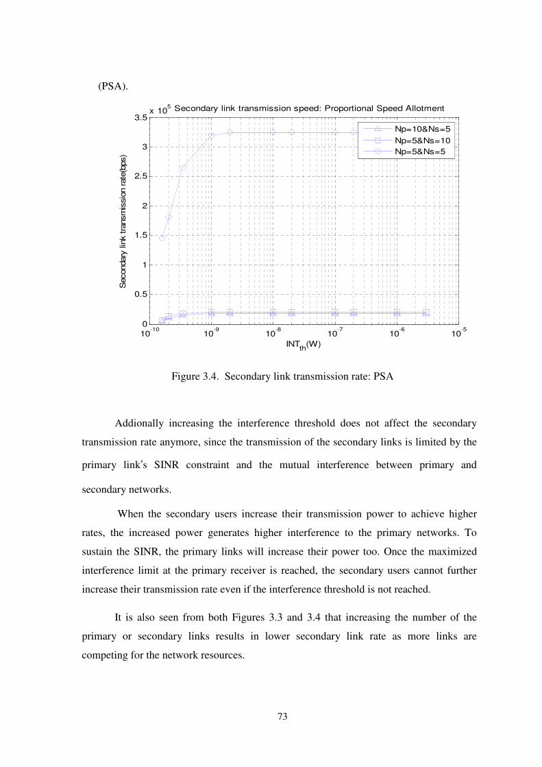
73

(PSA).

10-10

10-9

10-8

10-7

10-6

10-5

0

0.5

1

1.5

2

2.5

3

3.5x 10

5

INTth

(W)

Secondary

lin

k tra

nsm

issio

n rate

(bps)

Secondary link transmission speed: Proportional Speed Allotment

Np=10&Ns=5

Np=5&Ns=10

Np=5&Ns=5

Figure 3.4. Secondary link transmission rate: PSA

Addionally increasing the interference threshold does not affect the secondary

transmission rate anymore, since the transmission of the secondary links is limited by the

primary link’s SINR constraint and the mutual interference between primary and

secondary networks.

When the secondary users increase their transmission power to achieve higher

rates, the increased power generates higher interference to the primary networks. To

sustain the SINR, the primary links will increase their power too. Once the maximized

interference limit at the primary receiver is reached, the secondary users cannot further

increase their transmission rate even if the interference threshold is not reached.

It is also seen from both Figures 3.3 and 3.4 that increasing the number of the

primary or secondary links results in lower secondary link rate as more links are

competing for the network resources.

74

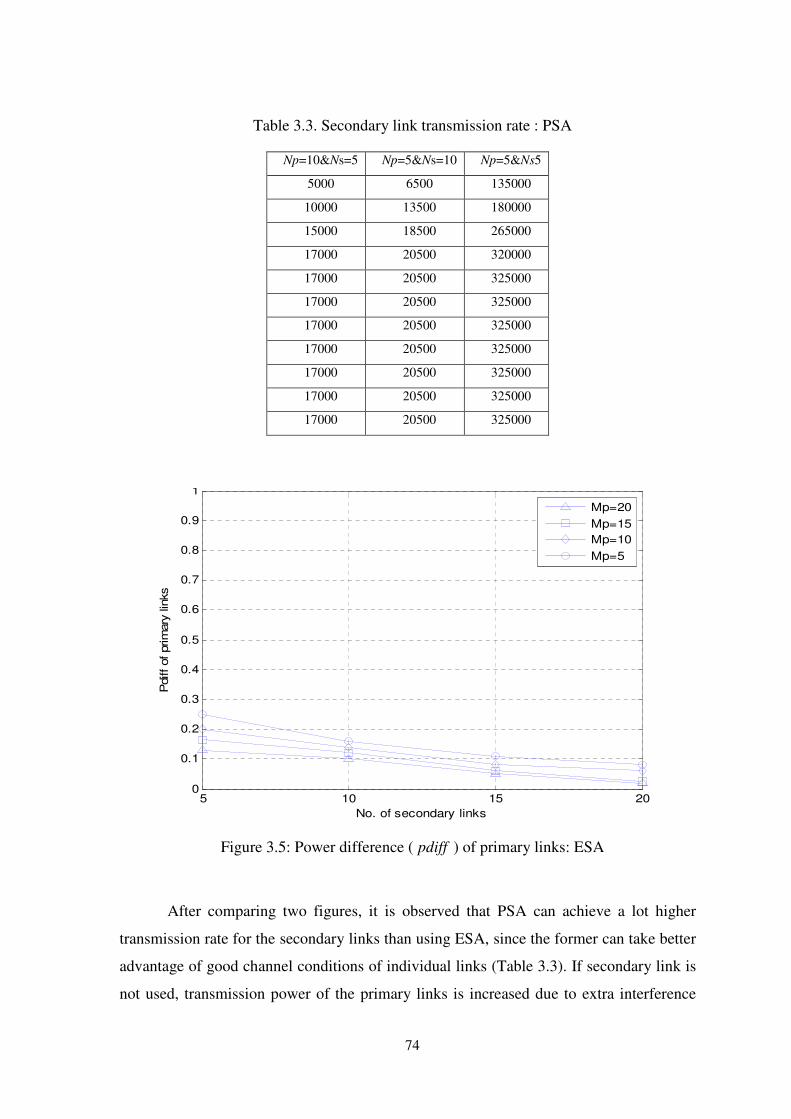
Table 3.3. Secondary link transmission rate : PSA

Np=10&Ns=5 Np=5&Ns=10 Np=5&Ns5

5000 6500 135000

10000 13500 180000

15000 18500 265000

17000 20500 320000

17000 20500 325000

17000 20500 325000

17000 20500 325000

17000 20500 325000

17000 20500 325000

17000 20500 325000

17000 20500 325000

5 10 15 200

0.1

0.2

0.3

0.4

0.5

0.6

0.7

0.8

0.9

1

No. of secondary links

Pdiff of prim

ary

lin

ks

Mp=20

Mp=15

Mp=10

Mp=5

Figure 3.5: Power difference ( pdiff ) of primary links: ESA

After comparing two figures, it is observed that PSA can achieve a lot higher

transmission rate for the secondary links than using ESA, since the former can take better

advantage of good channel conditions of individual links (Table 3.3). If secondary link is

not used, transmission power of the primary links is increased due to extra interference

75

from the secondary links. pdiff is defined as the difference of the average transmission

power of the primary links with and without the secondary transmissions.

Figure. 3.5 (Table 3.4) shows that with the increase of the number of secondary

links, the average primary transmission power of the primary links decreases. This is

explained by the dramatic decrease of the secondary link transmission rate as the number

of secondary links increases.

Table 3.4: Power difference of primary links: ESA

MP=20 MP=15 MP=10 MP=5

0.13 0.165 0.2 0.25

0.1 0.12 0.13 0.16

0.05 0.06 0.08 0.11

0.02 0.025 0.06 0.08

Figure 3.6 :Power difference of primary links:PSA

Because of the equal rate allocation, the transmission rate of the secondary links is

5 10 15 200

1

2

3

4

5

6

7

8

9

10

No. of secondary links

Pdiff of prim

ary

lin

ks

power difference of primary links: PSA

Mp=5

Mp=10

Mp=15

Mp=20

76

limited by the link with the worst link condition. ( Table 3.5).

Figure 3.6 shows that, pdiff of the primary links decrease with the number of

secondary links for PSA.With the same amount of pdiff , the CRN based on PSA can

achieve much higher transmission rate than that based on ESA.

Table 3.5: Power difference for diff. Values of MP

Figure 3.7- 3.9 shows ,maxpINT versus different system parameters. The actual

average interference at the primary link is also shown for ESA and PSA, respectively

200 400 600 800 1000 1200 1400 1600 1800 200010

-10

10-9

10-8

10-7

10-6

10-5

10-4

Dmax

(m)

Inte

rfere

nce to P

rim

ary

Lin

ks(W

)

Maximum interference vs. cell size

PSA

ESA

INTp,max

Figure 3.7. Highest interference vs. Cell size

It is seen that a primary network with a smaller cell size, larger max,pP or larger

Mp=20 Mp=15 Mp=10 Mp=5

2.5 1.8 1.3 0.8

2.2 1.6 1.2 0.6

2.1 1.5 1.1 0.5

2.0 1.4 1.0 0.4

77

fading deviation may tolerate a larger interference threshold for the same number of

secondary links ( Table 3.6, 3.7 and 3.8).

Table 3.6: maxINT For PSA and ESA related to cell size

Most importantly, the figures show that PSA can cause significantly lower

interference to the primary links than ESA. With ESA, the link with the worst SINR

condition may transmit much higher power than other links. When this link is close to the

primary link receiver (the BS), the primary link transmitters should transmit very high

power to combat the high interference.

Therefore, in ESA, it is more likely that the primary link transmitters reach the

maximum transmission power limit. This also explains that the interference level at the

BS using ESA is almost the same as,maxp

INT . In contrast, PSA does not encourage the

secondary links with poor SINR to transmit as high rate as the links with good SINR, and

therefore the interference level at the primary links is limited by the maximum

transmission power of both the primary and secondary transmitters.

PSA ESA maxINT

1.00E05 2.80E05 3.00E05

2.50E07 3.00E06 3.10E06

1.50E08 3.00E07 3.20E07

3.00E09 7.00E08 9.00E08

8.00E10 1.30E08 1.80E08

78

0.2 0.3 0.4 0.5 0.6 0.7 0.8 0.9 10

0.5

1

1.5

2

2.5

3

3.5

4

4.5x 10

-7

Pmax

(W)

Inte

rfere

nce t

o p

rim

ary

lin

ks

Maximum interference vs Pp,max

PSA

ESA

INTp,max

Figure 3.8: Maximum interference vs. max,pP

Table 3.7:,maxp

INT for PSA and ESA related to max,pP

ESA PSA ,maxpINT

1.00E08 1.20E07 1.26E07

1.10E08 1.60E07 1.63E07

1.20E08 2.00E07 2.11E07

1.30E08 2.50E07 2.50E07

1.60E08 3.00E07 2.90E07

1.80E08 3.50E07 3.3507

2.20E08 3.00E07 3.80E07

79

2 3 4 5 6 7 80

0.5

1

1.5

2

2.5

3

3.5

4x 10

-7

sigma(db)

Inte

rfere

nce to P

rim

ary

Lin

ks(W

)

Maximum interference vs sigma

PSA

ESA

INTp,max

Figure 3.9 :Maximum interference vs. Sigma

Table 3.8: ,maxp

INT for PSA and ESA

PSA ESA ,maxpINT

1.00E08 6.00E08 6.60E08

8.00E09 9.50E08 9.50E08

1.10E08 1.30E07 1.28E07

1.90E08 1.60E07 1.62E07

3.00E08 2.00E07 2.10E07

6.00E08 2.70E07 2.75E07

1.00E07 3.70E07 3.80E07

Transmission rate of the secondary links is shown in Fig. 3.10 based on the two

interference models defined in (3.3) and (3.4).

The difference is more obvious when thINT is small and close to the noise power

level. When thINT is relatively large, the two interference models do not make obvious

difference to the secondary transmission rate (Table 3.9).

80

10-10

10-9

0

1

2

3

4

5

6

7

8

9

10x 10

7

INTth

(W)

Secondary

lin

k tra

nsm

issio

n rate

(bps)

Comparision of two interference models

Interference Model I

Interference Model II

Figure 3.10: Comparison of two interference models

Table 3.9: Comparison of interference model 1 and 2.

INTth Interference Model I Interference Model II

1.00E-10 0 0 31000000 50000000

2.00E-10 32000000 31000000 32000000 65000000

3.00E-10 35000000 70000000 38000000 75000000

3.00E-10 51000000 79000000 52000000 80000000

7.00E-10 60000000 86000000 60500000 87000000

1.00E-09 61000000 88000000 61500000 89000000

When thINT is small, using the second interference model achieves much higher

transmission rate than using the first interference model, since in the latter case, noise

and interference from the primary network can dominate the interference threshold,

while in first interference model, the secondary transmissions can take advantage of all

the interference allowed by thINT .

81

As thINT increases, the secondary transmission power increases and eventually

is limited by their mutual interference and SINR constraints, but not by thINT . At this

point, the two interference models result in about the same transmission rate at the

secondary network.

3.5.2. Joint Admission Control and Packet Transmission Scheduling in

CRNs

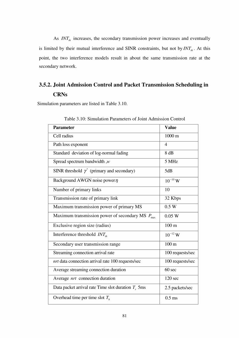
Simulation parameters are listed in Table 3.10.

Table 3.10: Simulation Parameters of Joint Admission Control

Parameter Value

Cell radius 1000 m

Path loss exponent 4

Standard deviation of log-normal fading 8 dB

Spread spectrum bandwidth ,w 5 MHz

SINR threshold *γ (primary and secondary) 5dB

Background AWGN noise powerη 1010− W

Number of primary links 10 Transmission rate of primary link 32 Kbps

Maximum transmission power of primary MS 0.5 W

Maximum transmission power of secondary MS maxP 0.05 W

Exclusive region size (radius) 100 m

Interference threshold thINT 1210− W

Secondary user transmission range 100 m

Streaming connection arrival rate 100 requests/sec nrt data connection arrival rate 100 requests/sec 100 requests/sec

Average streaming connection duration 60 sec

Average nrt connection duration 120 sec

Data packet arrival rate Time slot duration sT 5ms 2.5 packets/sec

Overhead time per time slot hT 0.5 ms

82

For the CRN, two independent Poisson processes are used to generate the

connection requests for the streaming traffic and nrt data traffic, respectively. The new

connection is randomly (with equal possibility) assigned to one of the transmitter-receiver

pairs that do not have active connections at the time. The duration of each admitted

connection follows an exponential distribution. For each admitted nrt connection, data

packets each with a fixed size are generated using another Poisson process.

Figure 3.11 demonstrates that setting different values for datathINT , can change the

relative amounts of the streaming and nrt traffic admitted into the system. When

datathINT , =0, all the system resource is used for the streaming traffic.

As datathINT , increases, more nrt data connections and fewer streaming

connections can be admitted into the system. [61] (Table 3.11)

.

0 10 20 30 40 50 60 70 80 900

10

20

30

40

50

60

70

80

INTth,data

/INTth

(%)

Num

ber

of

adm

itte

d c

onnections

Effect of INTth,data

on amount of admitted traffic

streaming traffic,Rreq,i

=100kbps

nrt traffc,Rmin,i

=20kbps

Figure 3.11: Effect of ,th dataINT on amount of admitted traffic

83

Table 3.11: Streaming and nrt traffic

600 700 800 900 1000 1100 1200 1300 1400 15000

0.05

0.1

0.15

0.2

0.25

0.3

0.35

0.4

0.45

0.5

Average Duration (time slots),INTth

,data

/INTth

=30%(K=3)

P(R

av

r, dur/R

min

<1)

Cumlative avrage data throughput

VC=900

VC=600

VC=300

Figure 3.12: Cumulative average data throughput

Figure 3.12 shows performance of the nrt traffic where iavrR , in the vertical axis

is the cumulative average throughput of an admitted nrt connection over the time

interval indicated in the horizontal axis. (Table 3.12)

Streaming

traffic nrt traffic

20 0

18 18

16.5 22

15 28

13 35

11 32

10.5 53

10 63

9 70

8.9 78

84

Table 3.12: Different values of VC

It is shown that when the time interval is sufficiently long (about 1500 time slots

with the given parameters), all connections can receive their required average

throughput.

100 200 300 400 500 600 700 800 9000

0.2

0.4

0.6

0.8

1

1.2

1.4

1.6

1.8

2x 10

7

Virtual counter limit (time slots) INTth,data

/INTth

=30% (K=3)

Tra

nsm

issio

n e

ffic

iency(b

its p

er

slo

t)

Virtual

Distributed

Figure 3.13: Throughput and delay performance of nrt traffic

VC=900 VC=600 VC=300

0.3 0.39 0.51

0.23 0.3 0.37

0.16 0.22 0.26

0.1 0.15 0.19

0.07 0.1 0.125

0.05 0.07 0.09

0.03 0.05 0.065

0.02 0.03 0.035

0.01 0.02 0.035

0 0.01 0.015

85

Figure.3.13 shows performance of the nrt traffic when using the weight-based

scheduling, where iavrR , in the vertical axis is the cumulative average throughput of an

admitted nrt connection over the time interval indicated in the horizontal axis. It is

shown that when the time interval is sufficiently long (about 1500 time slots with the

given parameters), all connections can receive their required average throughput.

Within a short period of time, using smaller maxξ may result in smoother rate

changes since it forces the nrt connections to transmit more frequently. On the other

hand, setting a larger value for maxξ may benefit the system resource utilization. Within

a short period of time, using smaller maxξ may result in smoother rate changes since it

forces the nrt connections to transmit more frequently. The packet transmission delay

and throughput performance of the admitted nrt traffic is evaluated in figure 3.13. The

figure shows that the performance of the optimum scheduling and the weight-based

scheduling is quite close, in terms of both throughput and delay. This shows the

effectiveness of the weight-based scheduling. (Table 3.13)

Table 3.13: Comparison between Virtual and Distributed values

The connection dropping rates are shown in figure 3.14. It shows that as maxξ

increases, the throughput increases, while data transmission delays increases too. This

shows the tradeoff between the resource utilization and the latency (refer Table 3.14). It

is seen that it is possible to achieve very low connection dropping rate.

Virtual Distributed

2000000 2200000

3300000 3500000

3300000 3500000

5300000 5500000

6300000 6300000

7100000 7300000

8000000 8300000

8500000 8900000

9000000 9300000

86

Figure 3.14: Connection dropping rate

The criterion that drops the most recent admitted connection, does not consider the

interference condition and therefore results in the highest dropping rate, and the criterion

based on primary to secondary interference achieves drop rate performance between the

other two criteria. (Table 3.14)

Table 3.14: Connection dropping rate for different values of M

M=5,smallest

Weight

M=15,smallest

weight

M=5,worst

gain

M=15,worst

gain

M=5,recently

accepted

M=5,recently

accepted

0 0 0.0001 0.0005 0.00058 0.0006

0.0001 0.0001 0.0002 0.0008 0.001 0.0012

0.0002 0.0002 0.00029 0.0011 0.00135 0.0019

0.00028 0.00035 0.00039 0.00155 0.00199 0.0025

0.00038 0.00055 0.0007 0.0021 0.0026 0.0032

0.0007 0.00082 0.00098 0.0026 0.0033 0.003

0.00087 0.00115 0.0015 0.0032 0.0031 0.0038

0.0012 0.00138 0.0021 0.0038 0.0038 0.0058

0.0016 0.0019 0.0028 0.0036 0.0058 0.0072

0.02 0.03 0.04 0.05 0.06 0.07 0.08 0.09 0.10

1

2

3

4

5

6

7

8x 10

-3

Probability from "off" to "on"

Connection d

ropin

g r

ate

Connection droping rate

M=5,Drop link with smallest weight

M=15,Drop link with smallest weight

M=5,Drop link with worst link gain

M=15,Drop link with worst link gain

M=5,Drop most recently accepted

M=15,Drop most recently accepted

87

3.6. Conclusion

Interference model for scheduling algorithm in CDMA based CNR is designed The

actual average interference at the primary link is also shown for ESA and PSA,

respectively. Results indicate that there is a limit on the interference threshold beyond

which the secondary link transmission rate cannot be increased by increasing the

interference threshold. Also, the increase of the secondary user transmission rate will

consume additional power from the primary user, and the same amount of power increase

from the primary users can support higher rate of the secondary links using proportional

rate allocation, compared to using equal rate allocation among the secondary links.

In contrast, PSA does not encourage the secondary links with poor SINR to

transmit as high rate as the links with good SINR, and therefore the interference level at

the primary links is limited by the maximum transmission power of both the primary and

secondary transmitters.

A throughput computation scheme for real-time data traffic is proposed and

scheduling schemes for each type of the traffic are designed. By using static channel and

interference conditions, the admission control scheme effectively limits amount of the

traffic admitted into the system to be below capacity. The heuristic scheduling scheme

opportunistically takes gain of the random channel and interference conditions and

achieves low and fair session outage probability for the streaming traffic and high

throughput and fair transmission delay for the data traffic, and its performance is close to

the optimum scheduling. In this way, analysis of the optimum power and rate

allocations in a CDMA-based cognitive wireless network with spectrum underlay is done.

Comparison of two interference models is discussed.

Our analysis indicates that there is a limit on the interference threshold beyond

which the secondary link transmission rate cannot be increased by increasing the

interference threshold. Furthermore, the increase of the secondary user transmission rate

will consume extra power from the primary user, and the same amount of power increase

from the primary users can support higher rate of the secondary links using proportional

speed allocation (PSA), compared to equal speed allocation (ESA) among the secondary

links.