
Radio Resource Management for Quality of Experience ... · Radio Resource Management for Quality of...
64
FEDERAL UNIVERSITY OF CEARÁ DEPARTMENT OF TELEINFORMATICS ENGINEERING POSTGRADUATE PROGRAM IN TELEINFORMATICS ENGINEERING Radio Resource Management for Quality of Experience Optimization in Wireless Networks Master of Science Thesis Author Victor Farias Monteiro Advisor Prof. Dr. Francisco Rodrigo Porto Cavalcanti Co-Advisor Prof. Dr. Tarcisio Ferreira Maciel FORTALEZA –CEARÁ JULY 2015
-
Upload
nguyentuyen -
Category
Documents
-
view
227 -
download
2
Transcript of Radio Resource Management for Quality of Experience ... · Radio Resource Management for Quality of...
FEDERAL UNIVERSITY OF CEARÁ
DEPARTMENT OF TELEINFORMATICS ENGINEERING
POSTGRADUATE PROGRAM IN TELEINFORMATICS ENGINEERING
Radio Resource Management for Quality of
Experience Optimization in Wireless Networks
Master of Science Thesis
Author
Victor Farias Monteiro
Advisor
Prof. Dr. Francisco Rodrigo Porto Cavalcanti
Co-Advisor
Prof. Dr. Tarcisio Ferreira Maciel
FORTALEZA – CEARÁ
JULY 2015
UNIVERSIDADE FEDERAL DO CEARÁ
DEPARTAMENTO DE ENGENHARIA DE TELEINFORMÁTICA
PROGRAMA DE PÓS-GRADUAÇÃO EM ENGENHARIA DE TELEINFORMÁTICA
Gestão de Recursos de Rádio para Otimização da
Qualidade de Experiência em Sistemas Sem Fio
Autor
Victor Farias Monteiro
Orientador
Prof. Dr. Francisco Rodrigo Porto Cavalcanti
Co-orientador
Prof. Dr. Tarcisio Ferreira Maciel
Dissertação apresentada à Coordenação do
Programa de Pós-graduação em Engenharia
de Teleinformática da Universidade Federal
do Ceará como parte dos requisitos para
obtenção do grau de Mestre em Engenhariade Teleinformática. Área de concentração:
Sinais e sistemas.
FORTALEZA – CEARÁ
JULHO 2015
Dados Internacionais de Catalogação na Publicação
Universidade Federal do Ceará
Biblioteca de Pós-Graduação em Engenharia - BPGE
M78r Monteiro, Victor Farias.
Radio resource management for quality of experience optimization in wireless networks / Victor
Farias Monteiro. – 2015.
62 f. : il. color. , enc. ; 30 cm.
Dissertação (mestrado) – Universidade Federal do Ceará, Centro de Tecnologia, Departamento de
Engenharia de Teleinformática, Programa de Pós-Graduação em Engenharia de Teleinformática,
Fortaleza, 2015.
Área de concentração: Sinais e Sistemas.
Orientação: Prof. Dr. Francisco Rodrigo Porto Cavalcanti.
Orientação: Prof. Dr. Tarcísio Ferreira Maciel.
1. Teleinformática. 2.Alocação de potência. 3. Experiência - Qualidade. I. Título.
CDD 621.38


This page was intentionally left blank
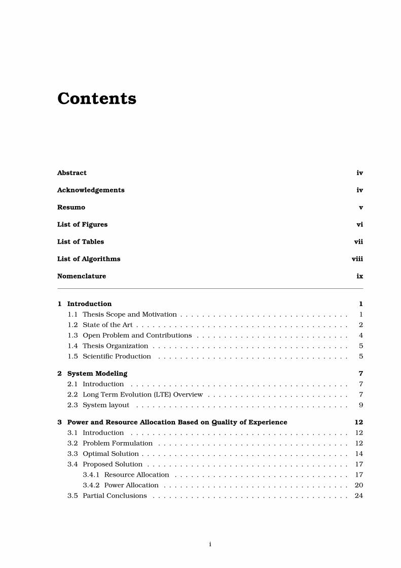
Contents
Abstract iv
Acknowledgements iv
Resumo v
List of Figures vi
List of Tables vii
List of Algorithms viii
Nomenclature ix
1 Introduction 1
1.1 Thesis Scope and Motivation . . . . . . . . . . . . . . . . . . . . . . . . . . . . . . . 1
1.2 State of the Art . . . . . . . . . . . . . . . . . . . . . . . . . . . . . . . . . . . . . . . 2
1.3 Open Problem and Contributions . . . . . . . . . . . . . . . . . . . . . . . . . . . . 4
1.4 Thesis Organization . . . . . . . . . . . . . . . . . . . . . . . . . . . . . . . . . . . . 5
1.5 Scientific Production . . . . . . . . . . . . . . . . . . . . . . . . . . . . . . . . . . . 5
2 System Modeling 7
2.1 Introduction . . . . . . . . . . . . . . . . . . . . . . . . . . . . . . . . . . . . . . . . 7
2.2 Long Term Evolution (LTE) Overview . . . . . . . . . . . . . . . . . . . . . . . . . . 7
2.3 System layout . . . . . . . . . . . . . . . . . . . . . . . . . . . . . . . . . . . . . . . 9
3 Power and Resource Allocation Based on Quality of Experience 12
3.1 Introduction . . . . . . . . . . . . . . . . . . . . . . . . . . . . . . . . . . . . . . . . 12
3.2 Problem Formulation . . . . . . . . . . . . . . . . . . . . . . . . . . . . . . . . . . . 12
3.3 Optimal Solution . . . . . . . . . . . . . . . . . . . . . . . . . . . . . . . . . . . . . . 14
3.4 Proposed Solution . . . . . . . . . . . . . . . . . . . . . . . . . . . . . . . . . . . . . 17
3.4.1 Resource Allocation . . . . . . . . . . . . . . . . . . . . . . . . . . . . . . . . 17
3.4.2 Power Allocation . . . . . . . . . . . . . . . . . . . . . . . . . . . . . . . . . . 20
3.5 Partial Conclusions . . . . . . . . . . . . . . . . . . . . . . . . . . . . . . . . . . . . 24
i
4 Performance Evaluation 25
4.1 Introduction . . . . . . . . . . . . . . . . . . . . . . . . . . . . . . . . . . . . . . . . 25
4.2 Simulation Assumptions . . . . . . . . . . . . . . . . . . . . . . . . . . . . . . . . . 25
4.3 Results . . . . . . . . . . . . . . . . . . . . . . . . . . . . . . . . . . . . . . . . . . . 27
4.3.1 Single Service Plan . . . . . . . . . . . . . . . . . . . . . . . . . . . . . . . . . 27
4.3.2 Multiple Service Plans . . . . . . . . . . . . . . . . . . . . . . . . . . . . . . . 31
4.3.3 Low Coverage Scenario . . . . . . . . . . . . . . . . . . . . . . . . . . . . . . 35
4.3.4 Imperfect Channel State Information (CSI) . . . . . . . . . . . . . . . . . . . 38
5 Conclusions and Future Work 41
Bibliography 43
ii

Acknowledgements
Though only my name appears on the cover of this work as author, so many people have
contributed to its production. I would like to offer my sincere thanks to all of them.
First and above all, I thank God for providing me this opportunity and granting me the
capability to successfully proceed.
A very special thanks goes out to my advisor, Prof. Fco. Rodrigo P. Cavalcanti, who
has confided in me since I was an undergraduate student. Four months ago, I was not even
thinking about defending this master thesis today (six months earlier than expected), but, with
his confidence in my potential and hard work, this became possible. Due to his experience,
he always brought a practical vision when I was most focused on technical problems.
I would like to express my most sincere gratitude to my co-advisor, Prof. Tarcisio F. Maciel.
The door of his office was always open whenever I ran into a trouble spot or had a question
about my research or writing. Thanks for devoting much time to reading my work over and
over again, I am really grateful for that.
I would also like to thank my friends from GTEL, Diego Sousa, Mairton, Yuri Victor, Hugo
Costa, Marciel Barros, Igor Osterno, Carlos Filipe, Darlan, Rafael Vasconcelos and Laszlon,
who have in some way contributed to the accomplishment of this work. To one of them, Diego
Sousa, I am indebted. He was busy with his own thesis and work, but squeezed time from
his schedule to give me helping hands as soon as I was in need. Important discussions and
improvements arose at lunchtime with him. I am also thankful to Prof. Fco. Rafael M. Lima,
who also helped me with technical advices and detailed reviews during my master degree, as
well as Prof. Emanuel B. Rodrigues.
It is said that friends are the family we choose, and I agree. Vitor Martins, Paulo Henrique,
Roberto Girão, Danilo Nóbrega, Lucas Sampaio, Thiago Fonseca, Italo Rolim, Vanessa Viana,
Luciana Borges and Camila Pio, among others, thank you for understanding when I was not
available for hanging out because of my studies.
Most important, none of this would have been possible without the love and patience of my
family. I am extremely grateful to my parents and my sister for their love, prayers, caring and
sacrifices for educating and preparing me for my future. Although they hardly understand
what I research on, they are willing to support every decision I make.
Finally, I acknowledge the technical and financial support from FUNCAP, Ericsson
Research, Wireless Access Network Department - Sweden, and Ericsson Innovation Center,
Brazil, under EDB/UFC.40 Technical Cooperation Contract.
Fortaleza, July 2015.
Victor Farias Monteiro
Abstract
A new generation of wireless networks, the 5th Generation (5G), is predicted for beyond
2020. For the 5G, it is foreseen an emerging huge number of services based on Machine-Type
Communications (MTCs) in different fields, such as, health care, smart metering and security.
Each one of them requiring different throughput rates, latency, processing capacity, energy
efficiency, etc.
Independently of the service type, the customers still need to get satisfied, which is
imposing a shift of paradigm towards incorporating the user as the most important factor
in wireless network management. This shift of paradigm drove the creation of the Quality of
Experience (QoE) concept, which describes the service quality subjectively perceived by the
users. QoE is generally evaluated by a Mean Opinion Score (MOS) ranging from 1 to 5.
In this context, QoE concepts can be considered with different objectives, such as,
increasing battery life, optimizing handover decision, enhancing access network selection
and improving Radio Resource Allocation (RRA). Regarding the RRA, in this master’s
thesis we consider QoE requirements when managing the limited available resources of a
communication system, such as frequency spectrum and transmit power. More specifically,
we study a radio resource assignment and power allocation problem that aims at maximizing
the minimum MOS of the users in a system subject to attaining a minimum number of
satisfied users.
Initially, we formulate a new optimization problem taking into account constraints on
the total transmit power and on the fraction of users that must be satisfied, which is an
important topic from an operator’s point of view. The referred problem is non-linear and
hard to solve. However, we get to transform it into a simpler form, a Mixed Integer Linear
Problem (MILP), that can be optimally solved using standard numerical optimization methods.
Due to the complexity of obtaining the optimal solution, we propose a heuristic solution to
this problem, called Power and Resource Allocation Based on Quality of Experience (PRABE).
We evaluate the proposed method by means of simulations and the obtained results show
that it outperforms some existing algorithms, as well as it performs close to the optimal
solution.
Keywords: Quality of Experience, Minimum Mean Opinion Score Maximization, Radio
Resource Allocation, Power Allocation.
iv
Resumo
Uma nova geração de sistemas de comunicações sem fio, 5a Geração (5G), é prevista para
2020. Para a 5G, é esperado o surgimento de diversos serviços baseados em comunicações
máquina à máquina em diferentes áreas, como assistência médica, segurança e redes de
medição inteligente. Cada um com diferentes requerimentos de taxa de transmissão, latência,
capacidade de processamento, eficiência energética, etc.
Independente do serviço, os clientes precisam ficar satisfeitos. Isto está impondo uma
mudança de paradigmas em direção à priorização do usuário como fator mais importante no
gerenciamento de redes sem fio. Com esta mudança, criou-se o conceito de qualidade de
experiência (do inglês, Quality of Experience (QoE)), que descreve de forma subjetiva como o
serviço é percebido pelo usuário. A QoE normalmente é avaliada por uma nota entre 1 e 5,
chamada nota média de opinião (do inglês, Mean Opinion Score (MOS)).
Neste contexto, conceitos de QoE podem ser considerados com diferentes objetivos, como:
aumentar a vida útil de baterias, melhorar a seleção para acesso à rede e aprimorar a alocação
dos recursos de rádio (do inglês, Radio Resource Allocation (RRA)). Com relação à RRA, nesta
dissertação consideram-se requerimentos de QoE na gestão dos recursos disponíveis em um
sistema de comunicações sem fio, como espectro de frequência e potência de transmissão.
Mais especificamente, estuda-se um problema de assinalamento de recursos de rádio e de
alocação de potência que objetiva maximizar a mínima MOS do sistema sujeito a satisfazer
um número mínimo de usuários pré-estabelecido.
Inicialmente, formula-se um novo problema de otimização considerando restrições quanto
à potência de transmissão e quanto à fração de usuários que deve ser satisfeita, o que é
um importante tópico do ponto de vista das operadoras. Este é um problema não linear e
de difícil solução. Ele é então reformulado como um problema linear inteiro e misto, que
pode ser resolvido de forma ótima usando algoritmos conhecidos de otimização. Devido à
complexidade da solução ótima obtida, propõe-se uma heurística chamada em inglês de
Power and Resource Allocation Based on Quality of Experience (PRABE). O método proposto
é avaliado por meio de simulações e os resultados obtidos mostram que sua performance é
superior à de outros existentes, sendo próxima à da ótima.
Palavras-Chave: Qualidade de Experiência, Maximização da Mínima MOS, Alocação de
Recursos de Rádio, Alocação de Potência.
v
List of Figures
1.1 Framework context. . . . . . . . . . . . . . . . . . . . . . . . . . . . . . . . . . . . . 4
2.1 LTE architecture. . . . . . . . . . . . . . . . . . . . . . . . . . . . . . . . . . . . . . 8
2.2 Time-frequency partition. . . . . . . . . . . . . . . . . . . . . . . . . . . . . . . . . . 9
2.3 Relationship between Signal to Noise Ratio (SNR), BLock Error Rate (BLER) and
Modulation and Coding Scheme (MCS) in Long Term Evolution (LTE) . . . . . . . 10
3.1 Studied problem. . . . . . . . . . . . . . . . . . . . . . . . . . . . . . . . . . . . . . . 13
3.2 Mode-2 unfolding of a third-order matrix. . . . . . . . . . . . . . . . . . . . . . . . 15
3.3 Flowchart of proposed resource assignment algorithm. . . . . . . . . . . . . . . . 19
3.4 Flowchart of proposed power allocation algorithm. . . . . . . . . . . . . . . . . . . 21
3.5 Flowchart of proposed power calculation to achieve a target MOS for a specific
user. . . . . . . . . . . . . . . . . . . . . . . . . . . . . . . . . . . . . . . . . . . . . 22
3.6 Flowchart of proposed power distribution targeting a uniform MOS. . . . . . . . 23
4.1 MOS function. . . . . . . . . . . . . . . . . . . . . . . . . . . . . . . . . . . . . . . . 26
4.2 Impact of the number of User Equipments (UEs) on the outage for satisfaction
factor, α, equal to 1. . . . . . . . . . . . . . . . . . . . . . . . . . . . . . . . . . . . . 28
4.3 Impact of the number of UEs on the minimum MOS for satisfaction factor, α,
equal to 1. . . . . . . . . . . . . . . . . . . . . . . . . . . . . . . . . . . . . . . . . . . 30
4.4 Impact of the satisfaction factor on the outage for number of UEs, U , equal to 20
and target MOS equal to 4.4. . . . . . . . . . . . . . . . . . . . . . . . . . . . . . . . 31
4.5 Impact of the target MOS of service 2, n2, on the outage for satisfaction factor
α1 = α2 = 1 and target MOS of service 1 n1 = 4.4. . . . . . . . . . . . . . . . . . . . 33
4.6 Impact of the target MOS of service 2, n2, on the outage for 10 UEs in each
service, U1 = U2 = 10, satisfaction factor α1 = 1 and target MOS of service 1
n1 = 4.4. . . . . . . . . . . . . . . . . . . . . . . . . . . . . . . . . . . . . . . . . . . . 34
4.7 Impact of the number of UEs on the outage for satisfaction factor, α, equal to 1. . 36
4.8 Impact of the satisfaction factor on the outage for number of UEs, U , equal to 20. 37
4.9 Impact of the degradation, ξ, on the outage for satisfaction factor, α, equal to 1
and number of UEs equal to 5. . . . . . . . . . . . . . . . . . . . . . . . . . . . . . . 39
4.10Impact of the degradation, ξ, on the outage for satisfaction factor, α, equal to 0.8. 40
vi
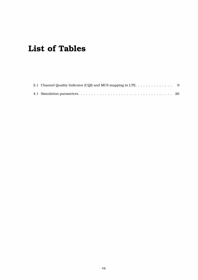
List of Tables
2.1 Channel Quality Indicator (CQI) and MCS mapping in LTE. . . . . . . . . . . . . . 9
4.1 Simulation parameters. . . . . . . . . . . . . . . . . . . . . . . . . . . . . . . . . . . 26
vii
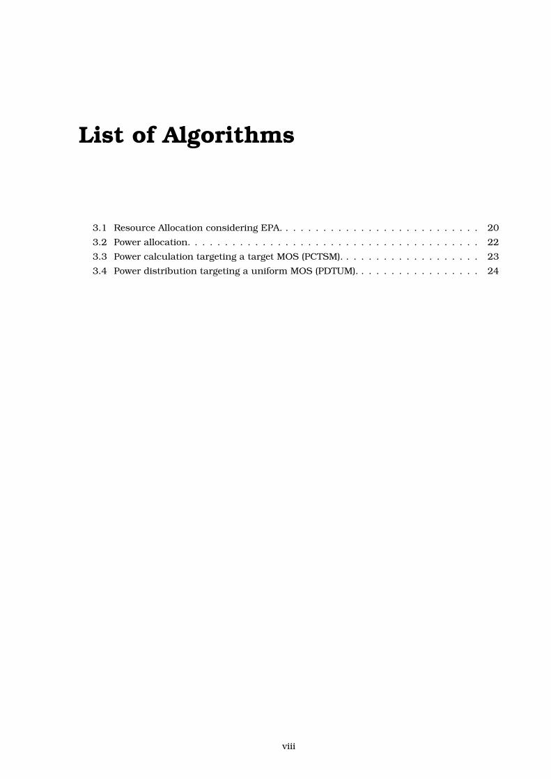
List of Algorithms
3.1 Resource Allocation considering EPA. . . . . . . . . . . . . . . . . . . . . . . . . . . 20
3.2 Power allocation. . . . . . . . . . . . . . . . . . . . . . . . . . . . . . . . . . . . . . . 22
3.3 Power calculation targeting a target MOS (PCTSM). . . . . . . . . . . . . . . . . . . 23
3.4 Power distribution targeting a uniform MOS (PDTUM). . . . . . . . . . . . . . . . . 24
viii
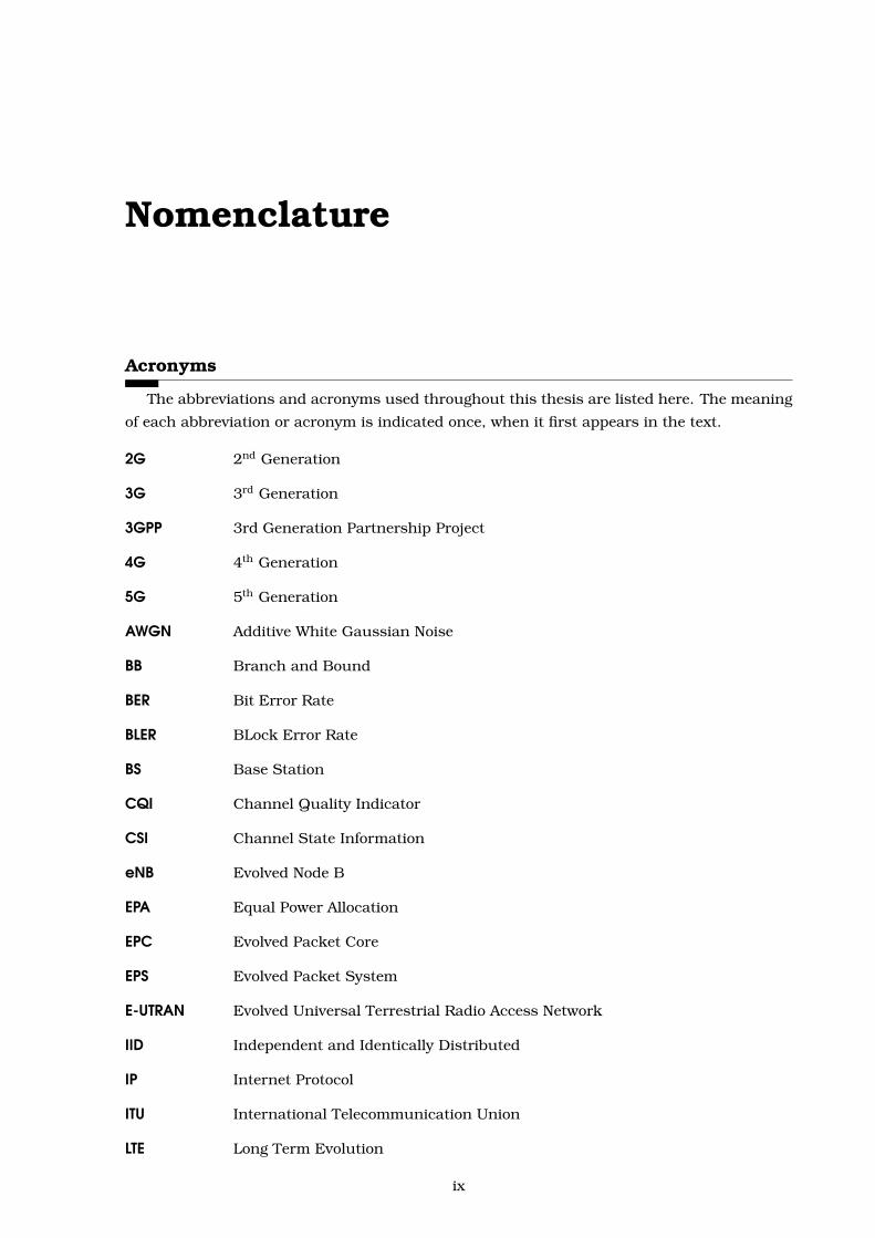
Nomenclature
Acronyms
The abbreviations and acronyms used throughout this thesis are listed here. The meaning
of each abbreviation or acronym is indicated once, when it first appears in the text.
2G 2nd Generation
3G 3rd Generation
3GPP 3rd Generation Partnership Project
4G 4th Generation
5G 5th Generation
AWGN Additive White Gaussian Noise
BB Branch and Bound
BER Bit Error Rate
BLER BLock Error Rate
BS Base Station
CQI Channel Quality Indicator
CSI Channel State Information
eNB Evolved Node B
EPA Equal Power Allocation
EPC Evolved Packet Core
EPS Evolved Packet System
E-UTRAN Evolved Universal Terrestrial Radio Access Network
IID Independent and Identically Distributed
IP Internet Protocol
ITU International Telecommunication Union
LTE Long Term Evolution
ix
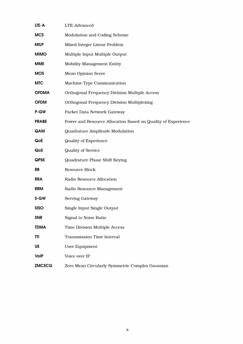
LTE-A LTE-Advanced
MCS Modulation and Coding Scheme
MILP Mixed Integer Linear Problem
MIMO Multiple Input Multiple Output
MME Mobility Management Entity
MOS Mean Opinion Score
MTC Machine-Type Communication
OFDMA Orthogonal Frequency Division Multiple Access
OFDM Orthogonal Frequency Division Multiplexing
P-GW Packet Data Network Gateway
PRABE Power and Resource Allocation Based on Quality of Experience
QAM Quadrature Amplitude Modulation
QoE Quality of Experience
QoS Quality of Service
QPSK Quadrature Phase Shift Keying
RB Resource Block
RRA Radio Resource Allocation
RRM Radio Resource Management
S-GW Serving Gateway
SISO Single Input Single Output
SNR Signal to Noise Ratio
TDMA Time Division Multiple Access
TTI Transmission Time Interval
UE User Equipment
VoIP Voice over IP
ZMCSCG Zero Mean Circularly Symmetric Complex Gaussian
x
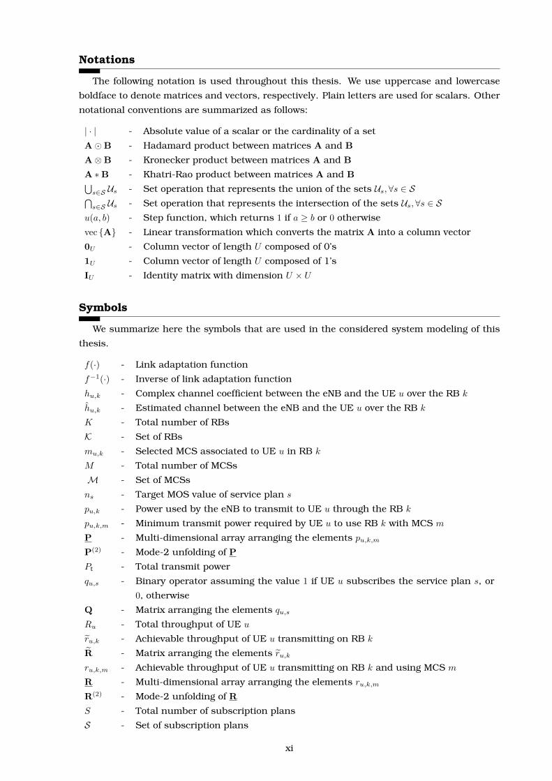
Notations
The following notation is used throughout this thesis. We use uppercase and lowercase
boldface to denote matrices and vectors, respectively. Plain letters are used for scalars. Other
notational conventions are summarized as follows:
| · | - Absolute value of a scalar or the cardinality of a set
A�B - Hadamard product between matrices A and B
A⊗B - Kronecker product between matrices A and B
A ∗B - Khatri-Rao product between matrices A and B⋃s∈S Us - Set operation that represents the union of the sets Us,∀s ∈ S⋂s∈S Us - Set operation that represents the intersection of the sets Us,∀s ∈ S
u(a, b) - Step function, which returns 1 if a ≥ b or 0 otherwise
vec {A} - Linear transformation which converts the matrix A into a column vector
0U - Column vector of length U composed of 0’s
1U - Column vector of length U composed of 1’s
IU - Identity matrix with dimension U × U
Symbols
We summarize here the symbols that are used in the considered system modeling of this
thesis.
f(·) - Link adaptation function
f−1(·) - Inverse of link adaptation function
hu,k - Complex channel coefficient between the eNB and the UE u over the RB k
hu,k - Estimated channel between the eNB and the UE u over the RB k
K - Total number of RBs
K - Set of RBs
mu,k - Selected MCS associated to UE u in RB k
M - Total number of MCSs
M - Set of MCSs
ns - Target MOS value of service plan s
pu,k - Power used by the eNB to transmit to UE u through the RB k
pu,k,m - Minimum transmit power required by UE u to use RB k with MCS m
P - Multi-dimensional array arranging the elements pu,k,mP(2) - Mode-2 unfolding of P
Pt - Total transmit power
qu,s - Binary operator assuming the value 1 if UE u subscribes the service plan s, or
0, otherwise
Q - Matrix arranging the elements qu,sRu - Total throughput of UE u
ru,k - Achievable throughput of UE u transmitting on RB k
R - Matrix arranging the elements ru,kru,k,m - Achievable throughput of UE u transmitting on RB k and using MCS m
R - Multi-dimensional array arranging the elements ru,k,mR(2) - Mode-2 unfolding of R
S - Total number of subscription plans
S - Set of subscription plans
xi
t - System minimum MOS
U - Total number of UEs
U - Set of UEs
Us - Total number of subscribers of service plan s
Us - Set of subscribers of service plan s
w - Vector arranging the variables of optimal solution
xu,k - Assignment index indicating whether the RB k is allocated to UE u
X - Matrix arranging the elements xu,kxu,k,m - Assignment index indicating whether the RB k is allocated to UE u using the
MCS m
X - Multi-dimensional array arranging the elements xu,k,mX(2) - Mode-2 unfolding of X
x(2) - Element of X(2)
αs - Satisfaction factor of service plan s
γu,k - Estimated instantaneous SNR of UE u on RB k
γu,k,m - Minimum estimated SNR that the eNB needs to transmit the information to UE
u in the RB k using the mth MCS and guaranteeing the desirable value of BLER
η - Channel estimation error
ξ - Degradation of the channel estimation
ρ - Matrix arranging the elements ρuρu - Binary operator assuming the value 1 if user u is satisfied or 0, otherwise
σ2 - Average AWGN power
τu - MOS of UE u
φ(·) - Function mapping rate into a MOS value
φ−1(·) - Inverse function of φ(·), it maps MOS values into corresponding required rate
values
ϕs - Minimum number of UEs that should be satisfied for service plan s
ϕ - Matrix arranging the elements ϕu
ψu - Required transmit rate for the UE u to be satisfied
ψ - Matrix arranging the elements ψs
xii
Chapter 1Introduction
This is an introductory chapter where we present the motivation and scope of this master’s
thesis in Section 1.1. After that, we present the state of the art of Quality of Experience
(QoE)-aware Radio Resource Allocation (RRA) methods in Section 1.2. The studied open
problems and the main contributions are stated in Section 1.3. Finally, the thesis organization
and the main scientific production during the Master course are presented in Sections 1.4 and
1.5, respectively.
1.1 Thesis Scope and Motivation
Different forecasts predict for beyond 2020 a new generation of wireless communications,
the 5th Generation (5G) [1–3]. For the 5G, it is foreseen a 1000 times higher mobile data
volume per unit area and a 10 to 100 times higher user data rate [2], as well as an emerging
huge number of services based on Machine-Type Communications (MTCs) in different fields,
such as, health care, smart metering and security.
In terms of Quality of Service (QoS), this diverse set of devices will ask for the support of
an evenly diverse range of communication requirements related to throughput, latency, and
packet loss ratio, among others. In this context, it will be difficult to define optimal throughput
or latency values, because these will change from service to service. Therefore, the operators
will increasingly need to focus on delivering high-quality service experience, independently of
technical requirements.
This leads us to the concept of QoE, which is defined in [4] as the overall acceptability of
an application or service, as perceived subjectively by the end-user. It is generally evaluated
by a Mean Opinion Score (MOS) ranging from 1 to 5 [5].
The overall goal of QoE management is to optimize end-user QoE (end-user perspective),
while making efficient use of network resources [6]. In order to successfully manage QoE
for a specific application, it is necessary to understand and identify multiple factors affecting
it (subjective and objectively) and how they impact QoE. Resulting QoE models dictate the
parameters to be monitored and measured. In [7], a survey breaks down the overall process
of QoE management into three general steps: QoE modeling, measurement and optimization.
QoE Modeling
Regarding the QoE modeling, its main objective is, given a set of conditions, to make
QoE estimations. For this, first of all, it is necessary to identify the influencing factors,
which, in [8], are grouped into four multidimensional spaces: Application (application
configuration-related factors), Resource (network/system related factors, e.g., throughput,
1.2. State of the Art 2
bandwidth, etc), Context (user’s environment, e.g., location, time of day, movement, etc.) and
User (characteristics of a human user, e.g., gender, age, education background, etc.).
The majority of works have been focused on identifying the relationship between QoE and
the network/system related factors. For this purpose, quality assessments are deployed. The
main idea is to expose users to a specific service, where they need to rate the quality of the
service. The rates are then averaged into MOS. The details are specified in [9].
Nevertheless, there is still not a consensus on this topic. For example, in [10], it is
formulated that QoS and QoE are connected through an exponential relationship, called IQX
hypothesis, whereas, in [11], it is inferred that, especially for Voice over IP (VoIP) and mobile
broadband scenarios, the users’ experience follows logarithmic laws.
QoE Measurement
The main challenges in the QoE measurement are related to 3 questions [7]: what to
collect? Where to collect? And when to collect?
Firstly, one needs to determine which data to acquire. This decision depends on the service
type been monitored and on the QoE model adopted to convert the influencing factors into
MOS.
Secondly, one needs to decide where to collect the data, which can be within the network, at
the client side, or both. According to [12], the best way to obtain an accurate QoE assessment
is to combine reported measures from the mobile device with network data. However, as
pointed in [6], monitoring at the client side can pose issues of users’ privacy.
Finally, one should determine when and how often to perform the data acquisition. This
depends of what is been monitored and of where the measures are been taking, since
computational complexity and battery life of mobile devices need to be considered.
QoE Optimization
Concerning optimization strategies, different objectives can be considered, such as,
increasing battery life [13], optimizing handover decision [14], enhancing access network
selection [15] and improving Radio Resource Management (RRM). Regarding the RRM, one
possible approach is to consider QoE requirements when managing the limited available
resources of a communication system, such as frequency spectrum and transmit power.
In this context, this work proposes an algorithm of RRA and power allocation aiming at
maximizing the minimum MOS subject to a minimum number of satisfied users, wherein the
MOS objectively quantifies the users’ QoE.
1.2 State of the Art
According to [16], RRA problems can be classified into different categories, such as
opportunistic and fair algorithms.
Opportunistic algorithms
This category of algorithms is more interested in the system overall than in the users
individually. They exploit the idea of giving priority to users with the best opportunities to
achieve a predefined goal, over the other users. Several algorithms use this approach with
different objectives such as: rate maximization and power consumption minimization.
Rate maximization algorithms aim at maximizing the total data rate of the system. In [17],
the authors develop an RRM scheme that exclusively assigns a sub-carrier to a user with the
highest channel gain on that sub-carrier which maximizes the system sum rate. However,
usually, the resources are allocated to the users that are close to the base station, whereas
1.2. State of the Art 3
edge users generally suffer from starvation and have very low data rates [18].
In a similar way, power consumption minimization algorithms tend to keep users with
bad channel conditions in starvation. In [19], a low computational algorithm is proposed
to minimize power consumption with Bit Error Rate (BER) and data rate constraints for
different types of services. Another power minimization problem is formulated in [20]
with a minimum user data rate constraint using integer programming and continuous
relaxation-based suboptimal solution methods.
Fair algorithms
The main objective of this category is to reach fairness between users, avoiding the
starvation of the opportunistic algorithms. The minimum rate maximization and Round Robin
are examples of this category.
In [21], a minimum rate maximization algorithm is proposed for the downlink of an
Orthogonal Frequency Division Multiplexing (OFDM) broadband system. By prioritizing users
with low data rate, it tends to overcome the problem of edge users’ starvation.
The Round Robin technique consists of scheduling the equal amount of resources for all
users in circular order. In [22], it is presented a comparison between a greedy scheduling and
an opportunistic Round Robin scheme for Multiple Input Multiple Output (MIMO) systems.
The results testify the fairness of this scheme.
The majority of RRA schemes in the literature considers QoS optimization criteria.
However, as previously explained, 5G networks will demand the management of a wide range
of QoS requirements. Therefore, new approaches based on user’s experience are needed since
QoS metrics would not reflect client perception of different applications anymore.
QoE-aware algorithms
In [23], the performance of three QoS-based RRA algorithms (max rate, max-min rate and
proportional fair) are compared in terms of QoE metrics (average QoE and geometric mean
QoE). The authors conclude that the QoE results need to be enhanced.
In fact, some authors have already addressed QoE aspects in RRA problems. A commonly
studied problem in this field is the maximization of the overall QoE. In [24], the allocation
problem is modeled as a bounded optimization problem to achieve the maximum overall QoE
with a constraint in total transmit power. In [25], a power allocation scheme, targeting
at maximizing QoE is proposed for video transmissions over MIMO systems. The problem
is decomposed into sub-problems and a bisection search algorithm is used to obtain their
optimal solutions.
In [26], a multicell coordination among multiple Base Stations (BSs) is investigated for
interference mitigation and overall QoE maximization. The problem is formulated as a local
cooperative game, where BSs are encouraged to cooperate with their peer nodes in the
adjacent cells when scheduling users and allocating power.
As the other opportunistic algorithms, the disadvantage of [24–26] is that they may penalize
users with poor link conditions. In [27], a similar problem is studied, but a penalty function is
also considered aiming at guaranteeing the fairness among users, besides of maximizing the
level of QoE in the system. Another strategy is adopted by the authors of [28] to overcome this
problem. They firstly allocate sub-carriers to all the users in order to guarantee their minimal
transmit rate requirement, then the remaining sub-carriers are allocated to the users who
can achieve the best QoE gain. In [29], a proportional fair scheduling is proposed considering
not only the users’ QoE maximization but as also the fairness among users.
In [30], the authors propose a QoE-aware scheduler that maximizes the average number of
1.3. Open Problem and Contributions 4
satisfied users. Their scheme needs the users’ participation informing their satisfaction over
a one-bit feedback.
Another studied problem is the maximization of the minimal MOS in the system. In [31],
a frequency spectrum assignment based on game theory together with a water-filling power
allocation is proposed. The system is modeled as a market place where, after a random
assignment, the users, in pairs, negotiate for the resources. The same problem is studied
in [32]. The Hungarian algorithm is used to assign frequency spectrum, and the optimal
solution of a Tchebycheff problem is used for the power allocation.
1.3 Open Problem and Contributions
As far as we know, the problem of maximizing the minimum MOS of the system considering
a satisfaction factor, i.e., a constraint on the minimum number of users that must be satisfied,
was not studied yet. This constraint is an important operator requirement and was considered
in other contexts [33–35]. In a real network, this fraction is a parameter defined by the
network operator.
First of all, we analyze the optimal solution of this problem, as a Mixed Integer Linear
Problem (MILP). Since it requires a high computational effort, we propose a heuristic solution
called Power and Resource Allocation Based on Quality of Experience (PRABE).
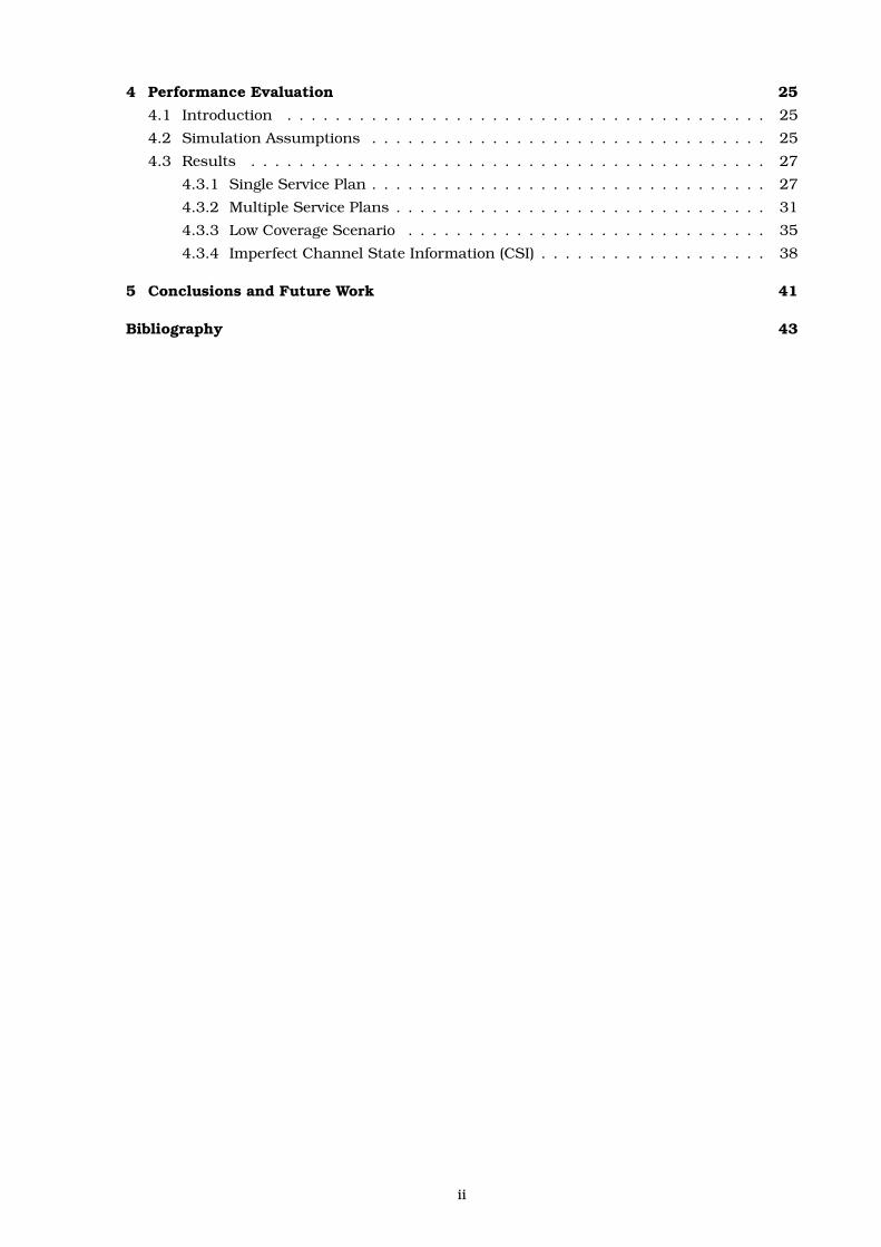
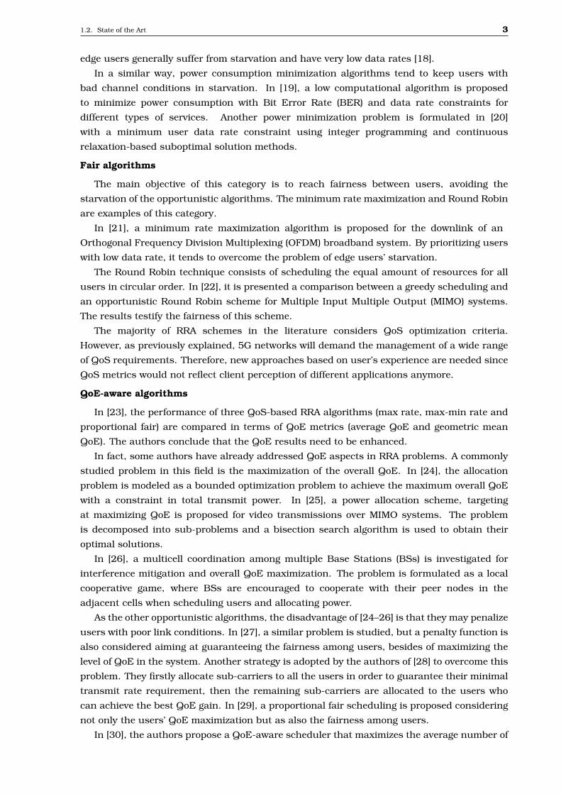
Figure 1.1 presents an overview of PRABE. The proposed framework is a QoE management
scheme which deals with MOS values. Independently of service or device, we consider
functions mapping QoS requirements into a MOS value. PRABE is divided into two parts:
the resource assignment and the power allocation. Each one of them tries first to satisfy the
required minimum number of satisfied users and then to maximize the minimum MOS in the
system.
QoS Requirements____________________________________________
QoS/ QoE Mapping
QoE Management
- Max-min system’s QoE- Minimum number of satisfied users
Resource Assignment Power Allocation
Services and Devices
QoS
Requirements_________________________________
Figure 1.1: Framework context.
In summary, the main contributions of this master’s thesis are:
i. Problem formulation: we formulate a max-min problem for the MOS considering a
satisfaction factor, an operator requirement not yet explored by previous works in this
context, as far as we know. With this constraint, we need to ensure that at least a specific
1.4. Thesis Organization 5
fraction of the total number of users meets a minimum MOS value.
ii. Characterization of optimal solution: the original problem has non-linear constraints
and may require a prohibitive computational effort. We transform it and solve it optimally
as a MILP using standard algorithms, with lower complexity.
iii. Proposal of heuristic solution: we propose a suboptimal solution including radio
resource assignment and power allocation requiring lower complexity than the optimal
one does.
iv. Performance evaluation: we show that the proposed heuristic outperforms
benchmarking solutions in the different analyzed scenarios, besides of performing close
to the optimal one.
1.4 Thesis Organization
In Chapter 2, we present the main assumptions in this thesis related to the system model,
which is based on 3rd Generation Partnership Project (3GPP)’s Long Term Evolution (LTE)
standards. To this end, we also provide a quick insight into some relevant features of LTE
and LTE-Advanced (LTE-A).
The mathematical formulation of the studied problem and its optimal solution as a MILP
are presented in Chapter 3. To overcome the problem of high computational effort required
by the optimal solution, we also present in this chapter a heuristic solution with lower
complexity, called PRABE.
The performance evaluation is presented in Chapter 4. We consider four different scenarios
to compare the performance of PRABE with two benchmarking algorithms besides of the
optimal solution and a mixed one. The mixed solution is composed by two parts an
optimal resource assignment considering Equal Power Allocation (EPA) and a heuristic power
allocation.
The main conclusions of this master’s thesis are summarized in Chapter 5. Furthermore,
we also point out the main research directions that can be considered as extension of this
work.
1.5 Scientific Production
The content and contributions presented in this Master’s thesis were submitted with the
following information:
I Victor F. Monteiro, Diego A. Sousa, Tarcisio F. Maciel, F. Rafael M. Lima, Emanuel
B. Rodrigues and F. Rodrigo P. Cavalcanti, “Radio Resource Allocation Framework for
Quality of Experience Optimization in Wireless Networks”. IEEE Network special issue -
QoE-Aware Design in Next-Generation Wireless Networks (submitted).
I Victor F. Monteiro, Diego A. Sousa, Tarcisio F. Maciel, F. Rafael M. Lima and F.
Rodrigo P. Cavalcanti, “Alocação de Recursos em Redes Sem Fio Baseada na Qualidade
de Experiência do Usuário”. XXXIII Brazilian Telecommunications Symposium (SBrT),
2015.
I Victor F. Monteiro, Diego A. Sousa, Tarcisio F. Maciel, F. Rafael M. Lima and F. Rodrigo
P. Cavalcanti, “Power and Resource Allocation Based on Quality of Experience”. IEEE
Transactions on Vehicular Technology (to be submitted).
1.5. Scientific Production 6
In parallel to the work developed in the Master course that was initiated on the first
semester of 2014, I have been working on other research projects related to analysis and
control of trade-offs involving QoS provision. In the context of these projects, I have
participated on the following papers and technical reports:
I Victor F. Monteiro, Diego A. Sousa, F. Hugo C. Neto, Emanuel B. Rodrigues, Tarcisio
F. Maciel and F. Rodrigo P. Cavalcanti, “Throughput-based Satisfaction Maximization
for a Multi Cell Downlink OFDMA System with Imperfect CSI”. XXXIII Brazilian
Telecommunications Symposium (SBrT), 2015.
I Diego A. Sousa, Victor F. Monteiro, Tarcisio F. Maciel and F. Rafael M. Lima, “Resource
Management for Rate Maximization with QoE Provisioning in Wireless Networks”. IEEE
Transactions on Vehicular Technology (submitted).
I Victor F. Monteiro, Diego A. Sousa, Tarcisio F. Maciel, F. Rafael M. Lima and F.
Rodrigo P. Cavalcanti, “Power and Resource Allocation Based on Quality of Experience”,
GTEL-UFC-Ericsson UFC.40, Tech. Rep., March 2015, First Technical Report.
I Diego A. Sousa, Victor F. Monteiro, Tarcisio F. Maciel and F. Rafael M. Lima, “Resource
Management for Rate Maximization with QoE Provisioning in Wireless Networks”,
GTEL-UFC-Ericsson UFC.40, Tech. Rep., March 2015, First Technical Report.
I F. Hugo C. Neto, Victor F. Monteiro, Diego A. Sousa, Emanuel B. Rodrigues, Tarcisio
F. Maciel and F. Rodrigo P. Cavalcanti, “A Novel Utility-Based Resource Allocation
Technique for Improving User Satisfaction in OFDMA Networks”, GTEL-UFC-Ericsson
UFC.33, Tech. Rep., Aug. 2014, Fourth Technical Report.
Chapter 2System Modeling
2.1 Introduction
The system architecture adopted in this thesis is based on 3rd Generation Partnership
Project (3GPP)’s Long Term Evolution (LTE) standards. To this end, Section 2.2 provides a
quick insight into some relevant features of LTE and LTE-Advanced (LTE-A) for the remaining
of this thesis. After that, in Section 2.3, we present the main assumptions of this thesis.
2.2 LTE Overview
With the development of highly advanced mobile devices, the demands for higher data
rates and better Quality of Service (QoS) increased rapidly. Therefore, in 2004 the 3GPP has
specified new standards for the mobile communications: the Evolved Universal Terrestrial
Radio Access Network (E-UTRAN) and the Evolved Packet Core (EPC), which define the radio
access network and the core network of the LTE system, respectively. The E-UTRAN together
with the EPC are known as the Evolved Packet System (EPS).
The standards for LTE are specified in the 3GPP Release 8, as high data rates of up to
300 Mbits/s in the downlink and 75 Mbits/s in the uplink. However, these specifications do
not meet the 4th Generation (4G) requirements set by the International Telecommunication
Union (ITU) such as data rate up to 1 Gbits/s. As a result, the LTE-A, an enhancement of
LTE, was presented as a 4G system to the ITU in 2009, and was finalized by the 3GPP in
Release 10 in March, 2011.
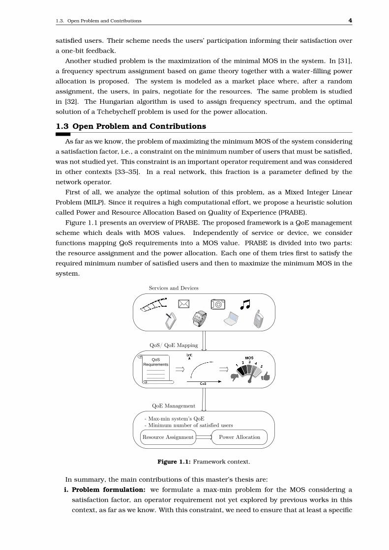
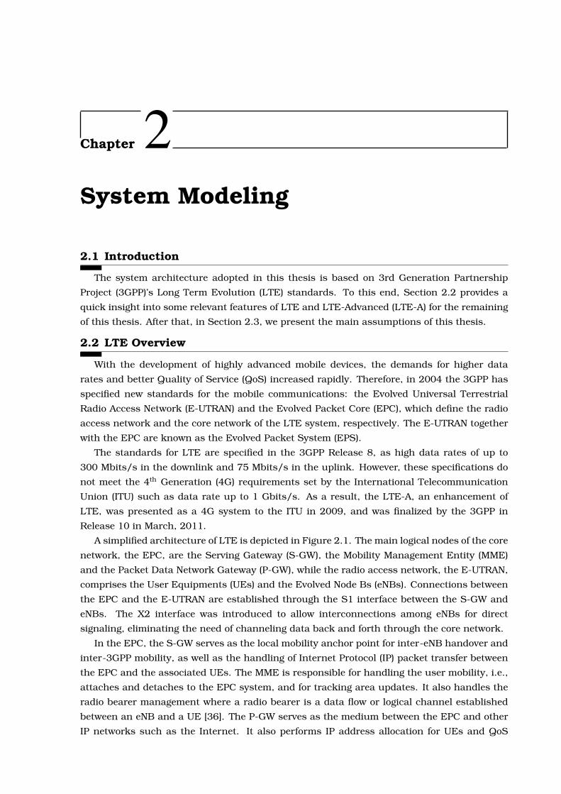
A simplified architecture of LTE is depicted in Figure 2.1. The main logical nodes of the core
network, the EPC, are the Serving Gateway (S-GW), the Mobility Management Entity (MME)
and the Packet Data Network Gateway (P-GW), while the radio access network, the E-UTRAN,
comprises the User Equipments (UEs) and the Evolved Node Bs (eNBs). Connections between
the EPC and the E-UTRAN are established through the S1 interface between the S-GW and
eNBs. The X2 interface was introduced to allow interconnections among eNBs for direct
signaling, eliminating the need of channeling data back and forth through the core network.
In the EPC, the S-GW serves as the local mobility anchor point for inter-eNB handover and
inter-3GPP mobility, as well as the handling of Internet Protocol (IP) packet transfer between
the EPC and the associated UEs. The MME is responsible for handling the user mobility, i.e.,
attaches and detaches to the EPC system, and for tracking area updates. It also handles the
radio bearer management where a radio bearer is a data flow or logical channel established
between an eNB and a UE [36]. The P-GW serves as the medium between the EPC and other
IP networks such as the Internet. It also performs IP address allocation for UEs and QoS
2.2. LTE Overview 8
Figure 2.1: LTE architecture.
enforcement [37].
Concerning the E-UTRAN, unlike the previous 2nd Generation (2G) and 3rd Generation
(3G) technologies, LTE integrates all the radio interface related functions into the eNB. The
eNB manages uplink and downlink transmissions among the UEs performing Radio Resource
Management (RRM) functions and control signaling.
Regarding the LTE physical layer of the downlink, some interesting concepts are relevant
for the remaining of this thesis, such as the Orthogonal Frequency Division Multiple Access
(OFDMA) technique and the link adaptation concept.
OFDMA
OFDMA is an extension of Orthogonal Frequency Division Multiplexing (OFDM). While
OFDM splits the frequency bandwidth into orthogonal sub-carriers and use them to transmit
data to a single user, OFDMA distributes sub-carriers to different users at the same time, so
that multiple users can be scheduled to receive data simultaneously. For LTE systems, the
sub-carrier spacing is 15 kHz.
The data symbols can be independently modulated and transmitted over these orthogonal
sub-carriers. In LTE, the available downlink modulation schemes are Quadrature Phase Shift
Keying (QPSK), 16-Quadrature Amplitude Modulation (QAM), and 64-QAM.
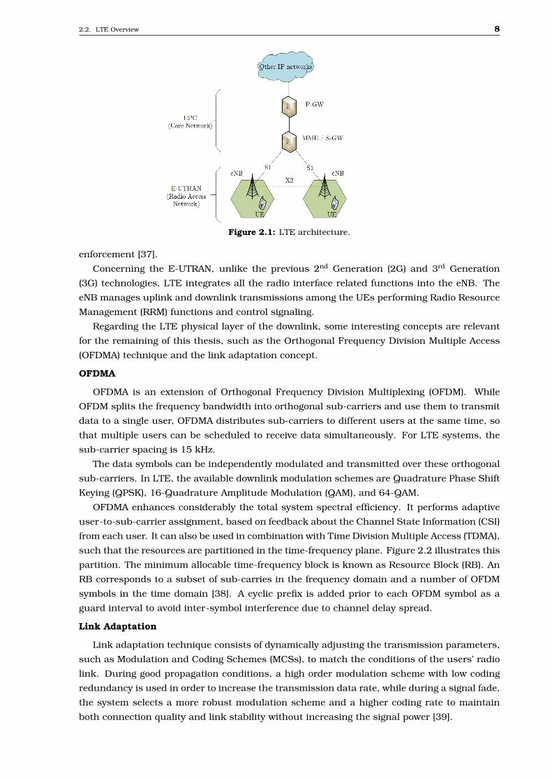
OFDMA enhances considerably the total system spectral efficiency. It performs adaptive
user-to-sub-carrier assignment, based on feedback about the Channel State Information (CSI)
from each user. It can also be used in combination with Time Division Multiple Access (TDMA),
such that the resources are partitioned in the time-frequency plane. Figure 2.2 illustrates this
partition. The minimum allocable time-frequency block is known as Resource Block (RB). An
RB corresponds to a subset of sub-carries in the frequency domain and a number of OFDM
symbols in the time domain [38]. A cyclic prefix is added prior to each OFDM symbol as a
guard interval to avoid inter-symbol interference due to channel delay spread.
Link Adaptation
Link adaptation technique consists of dynamically adjusting the transmission parameters,
such as Modulation and Coding Schemes (MCSs), to match the conditions of the users’ radio
link. During good propagation conditions, a high order modulation scheme with low coding
redundancy is used in order to increase the transmission data rate, while during a signal fade,
the system selects a more robust modulation scheme and a higher coding rate to maintain
both connection quality and link stability without increasing the signal power [39].
2.3. System layout 9
Figure 2.2: Time-frequency partition.
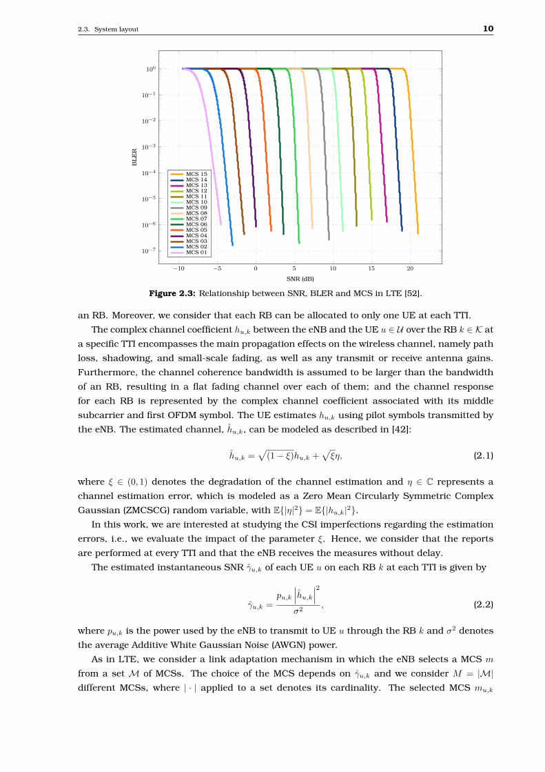
In LTE, the UEs transmit in the uplink the Channel Quality Indicator (CQI) to the eNB,
which, in response, selects the best adapted MCS to use in the downlink. Table 2.1 presents
the mapping of CQI into MCS in LTE. Note that larger CQI indexes, i.e., better channel
conditions, allow to transmit more bits on each OFDM symbol and to use the channel more
efficiently.
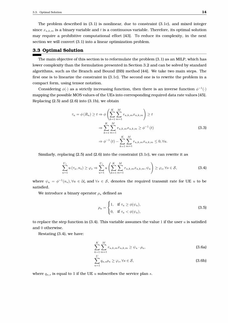
Differences in MCS bring different BLock Error Rate (BLER) performances, which can be
seen in Figure 2.3. It represents the relationship between Signal to Noise Ratio (SNR), BLER
and MCS. Note that for the same SNR, higher MCS index represents higher BLER, which
means that a given MCS requires a certain SNR to operate with an acceptably low BLER [40].
Table 2.1: CQI and MCS mapping in LTE [41].
CQIindex Modulation Code rate
(x 1024)Rate
(Bits/symbol)CQI
index Modulation Code rate(x1024)
Rate(Bits/symbol)
0 Out of range 8 16QAM 490 1.91411 QPSK 78 0.152 9 16QAM 616 2.40632 QPSK 120 0.234 10 64QAM 466 2.73053 QPSK 193 0.377 11 64QAM 567 3.32234 QPSK 308 0.602 12 64QAM 666 3.90235 QPSK 449 0.877 13 64QAM 772 4.52346 QPSK 602 1.176 14 64QAM 873 5.11527 16QAM 378 1.477 15 64QAM 948 5.5547
2.3 System layout
In this thesis, we consider the downlink of a LTE-like system composed of a single cell in
which an eNB is deployed to serve a set U of UEs distributed within its coverage area. Both the
eNB and the UEs are equipped with single antennas, i.e., we consider a Single Input Single
Output (SISO) scenario.
Due to the diversity of applications with distinct requirements, we consider that the UEs
are separated into different mobile subscription plans. We define S = {1, 2, . . . , S} as the set of
subscription plans and Us as the set of subscribers of service plan s ∈ S, where⋃
s∈S Us = U .
For example, a priority plan with higher requirements for emergency services, as fire brigade,
police and ambulances, and another one for UEs in general. Moreover, we consider that each
user subscribes to only a single service plan, i.e,⋂
s∈S Us = ∅.The considered LTE-like system employs OFDMA and TDMA as multiple access scheme,
where, due to signaling constraints, the radio resources are assigned in blocks. The system
disposes of K RBs arranged in a set K. The time duration corresponding to the time basis at
which resources are allocated to the UEs by the Radio Resource Allocation (RRA) algorithms
is termed herein as Transmission Time Interval (TTI), and it is equal to the time duration of
2.3. System layout 10
−10 −5 0 5 10 15 20
10−7
10−6
10−5
10−4
10−3
10−2
10−1
100
SNR (dB)
BLE
R
MCS 15MCS 14MCS 13MCS 12MCS 11MCS 10MCS 09MCS 08MCS 07MCS 06MCS 05MCS 04MCS 03MCS 02MCS 01
Figure 2.3: Relationship between SNR, BLER and MCS in LTE [52].
an RB. Moreover, we consider that each RB can be allocated to only one UE at each TTI.
The complex channel coefficient hu,k between the eNB and the UE u ∈ U over the RB k ∈ K at
a specific TTI encompasses the main propagation effects on the wireless channel, namely path
loss, shadowing, and small-scale fading, as well as any transmit or receive antenna gains.
Furthermore, the channel coherence bandwidth is assumed to be larger than the bandwidth
of an RB, resulting in a flat fading channel over each of them; and the channel response
for each RB is represented by the complex channel coefficient associated with its middle
subcarrier and first OFDM symbol. The UE estimates hu,k using pilot symbols transmitted by
the eNB. The estimated channel, hu,k, can be modeled as described in [42]:
hu,k =√(1− ξ)hu,k +
√ξη, (2.1)
where ξ ∈ (0, 1) denotes the degradation of the channel estimation and η ∈ C represents a
channel estimation error, which is modeled as a Zero Mean Circularly Symmetric Complex
Gaussian (ZMCSCG) random variable, with E{|η|2} = E{|hu,k|2}.In this work, we are interested at studying the CSI imperfections regarding the estimation
errors, i.e., we evaluate the impact of the parameter ξ. Hence, we consider that the reports
are performed at every TTI and that the eNB receives the measures without delay.
The estimated instantaneous SNR γu,k of each UE u on each RB k at each TTI is given by
γu,k =pu,k
∣∣∣hu,k∣∣∣2σ2
, (2.2)
where pu,k is the power used by the eNB to transmit to UE u through the RB k and σ2 denotes
the average Additive White Gaussian Noise (AWGN) power.
As in LTE, we consider a link adaptation mechanism in which the eNB selects a MCS m
from a set M of MCSs. The choice of the MCS depends on γu,k and we consider M = |M|different MCSs, where | · | applied to a set denotes its cardinality. The selected MCS mu,k
2.3. System layout 11
associated to UE u in RB k is given by
mu,k = f (γu,k) , (2.3)
where f(γu,k) is the link adaptation function. In this work, we consider that the eNB selects
as the best MCS for a given UE u on an RB k the one that leads to the highest data rate for a
given allocated power.
Fixing a desirable value of BLER, we can obtain from the link adaptation curves the
minimum estimated SNR, γu,k,m, that the eNB needs to transmit the information to UE u
in the RB k using the mth MCS and guaranteeing the desirable value of BLER. This minimum
SNR is given by
γu,k,m = f−1(mu,k), (2.4)
where f−1(·) is the inverse of link adaptation function.
From (2.4), we can obtain the values of γu,k,m, which can be used in (2.2) to obtain the
minimum transmit power, pu,k,m, associated to MCS m. Since we consider flat fading over
each RB, at each TTI, the value of hu,k in (2.2) is constant for each pair {u, k}.Defining ru,k,m as the throughput of UE u transmitting on RB k and using MCS m, the total
throughput Ru of UE u is given by
Ru =
K=|K|∑k=1
M=|M|∑m=1
ru,k,mxu,k,m, (2.5)
where xu,k,m is the assignment index indicating whether the RB k is allocated to UE u using
the MCS m.
Finally, the Quality of Experience (QoE) τu of a UE u can be obtained from the rate Ru using
the function φ(·), which maps rate into an Mean Opinion Score (MOS), as
τu = φ (Ru) . (2.6)
Based on all these assumptions, we are now able to introduce the studied problem, as well
as its solutions, which will be done in the next chapter.
Chapter 3Power and Resource Allocation
Based on Quality of Experience
3.1 Introduction
This chapter presents the problem studied in this master thesis and its solutions. The
mathematical formulation of the problem and its optimal solution as a Mixed Integer Linear
Problem (MILP) are presented in Sections 3.2 and 3.3, respectively. MILPs can be solved by
standard numerical optimization methods, nevertheless, they still require high computational
effort. To overcome this issue, a heuristic solution is proposed in Section 3.4.
3.2 Problem Formulation
As already mentioned, the operators are changing their focus to deliver services with high
Quality of Experience (QoE), independently of technical requirements, and measuring their
performance based on the percentage of satisfied users in the system.
In this context, we aim to assign Resource Blocks (RBs) to the User Equipments (UEs)
being served by the system and to allocate power to their corresponding channels in a way
that maximizes the minimum Mean Opinion Score (MOS) perceived by these same UEs. In
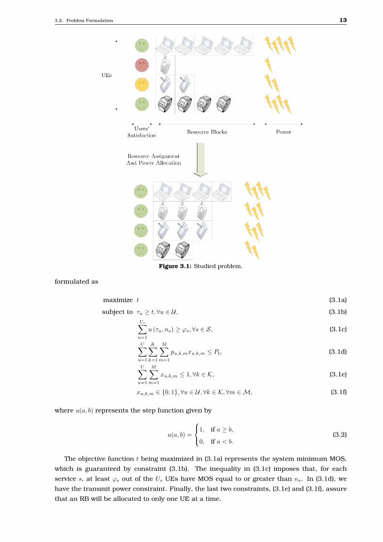
Figure 3.1 we have an illustration of the studied problem. Initially, the smartphone and tablet
users are unsatisfied due to the low number of RBs and power allocated to them, while the
notebook and smartwatch users have more RBs than they need to get satisfied. Then, the RBs
are reassigned and the power is reallocated between the UEs’ channels in order to maximize
the minimum satisfaction in the system.
Besides the maximization of the minimum MOS t, in order to guarantee a minimum quality
for the services being provided by the network operator, we require that at least ϕs UEs should
be satisfied for each service plan s, i.e, have a MOS equal to or higher than a given target MOS
value ns. We call the ratio αs =ϕs
Usas the satisfaction factor of the service plan s.
Moreover, our problem is also constrained in transmit power, which should be equal to
or lower than the total transmit power Pt available at the Evolved Node B (eNB). Based on
these assumptions and on the models presented in Section 2.3, this problem can then be
3.2. Problem Formulation 13
Figure 3.1: Studied problem.
formulated as
maximize t (3.1a)
subject to τu ≥ t,∀u ∈ U , (3.1b)Us∑u=1
u (τu, ns) ≥ ϕs,∀s ∈ S, (3.1c)
U∑u=1
K∑k=1
M∑m=1
pu,k,mxu,k,m ≤ Pt, (3.1d)
U∑u=1
M∑m=1
xu,k,m ≤ 1,∀k ∈ K, (3.1e)
xu,k,m ∈ {0, 1},∀u ∈ U ,∀k ∈ K,∀m ∈M, (3.1f)
where u(a, b) represents the step function given by
u(a, b) =
1, if a ≥ b,
0, if a < b.(3.2)
The objective function t being maximized in (3.1a) represents the system minimum MOS,
which is guaranteed by constraint (3.1b). The inequality in (3.1c) imposes that, for each
service s, at least ϕs out of the Us UEs have MOS equal to or greater than ns. In (3.1d), we
have the transmit power constraint. Finally, the last two constraints, (3.1e) and (3.1f), assure
that an RB will be allocated to only one UE at a time.
3.3. Optimal Solution 14
The problem described in (3.1) is nonlinear, due to constraint (3.1c), and mixed integer
since xu,k,m is a binary variable and t is a continuous variable. Therefore, its optimal solution
may require a prohibitive computational effort [43]. To reduce its complexity, in the next
section we will convert (3.1) into a linear optimization problem.
3.3 Optimal Solution
The main objective of this section is to reformulate the problem (3.1) as an MILP, which has
lower complexity than the formulation presented in Section 3.2 and can be solved by standard
algorithms, such as the Branch and Bound (BB) method [44]. We take two main steps. The
first one is to linearize the constraint in (3.1c). The second one is to rewrite the problem in a
compact form, using tensor notation.
Considering φ(·) as a strictly increasing function, then there is an inverse function φ−1(·)mapping the possible MOS values of the UEs into corresponding required data rate values [45].
Replacing (2.5) and (2.6) into (3.1b), we obtain
τu = φ (Ru) ≥ t⇒ φ
(K∑
k=1
M∑m=1
ru,k,mxu,k,m
)≥ t
⇒K∑
k=1
M∑m=1
ru,k,mxu,k,m ≥ φ−1 (t)
⇒ φ−1 (t)−K∑
k=1
M∑m=1
ru,k,mxu,k,m ≤ 0,∀u.
(3.3)
Similarly, replacing (2.5) and (2.6) into the constraint (3.1c), we can rewrite it as
Us∑u=1
u (τu, ns) ≥ ϕs ⇒Us∑u=1
u
(K∑
k=1
M∑m=1
ru,k,mxu,k,m, ψu
)≥ ϕs,∀s ∈ S, (3.4)
where ψu = φ−1(ns),∀u ∈ Us and ∀s ∈ S, denotes the required transmit rate for UE u to be
satisfied.
We introduce a binary operator ρu defined as
ρu =
1, if τu ≥ φ(ψu),
0, if τu < φ(ψu),(3.5)
to replace the step function in (3.4). This variable assumes the value 1 if the user u is satisfied
and 0 otherwise.
Restating (3.4), we have:
K∑k=1
M∑m=1
ru,k,mxu,k,m ≥ ψu · ρu, (3.6a)
U∑u=1
qu,sρu ≥ ϕs,∀s ∈ S, (3.6b)
where qu,s is equal to 1 if the UE u subscribes the service plan s.
3.3. Optimal Solution 15
In this way, (3.1) can be rewritten as:
maximize φ−1 (t) , (3.7a)
subject to φ−1 (t)−K∑
k=1
M∑m=1
ru,k,mxu,k,m ≤ 0,∀u ∈ U , (3.7b)
K∑k=1
M∑m=1
ru,k,mxu,k,m ≥ ψu · ρu, (3.7c)
U∑u=1
qu,sρu ≥ ϕs,∀s ∈ S, (3.7d)
U∑u=1
K∑k=1
M∑m=1
pu,k,mxu,k,m ≤ Pt, (3.7e)
U∑u=1
M∑m=1
xu,k,m ≤ 1,∀k ∈ K, (3.7f)
xu,k,m ∈ {0, 1},∀u ∈ U , k ∈ K,m ∈M. (3.7g)
At this point, we will reformulate (3.7) in a matrix form. For this, we need to introduce
some concepts and definitions related to tensors. The first one is the concept of unfolding,
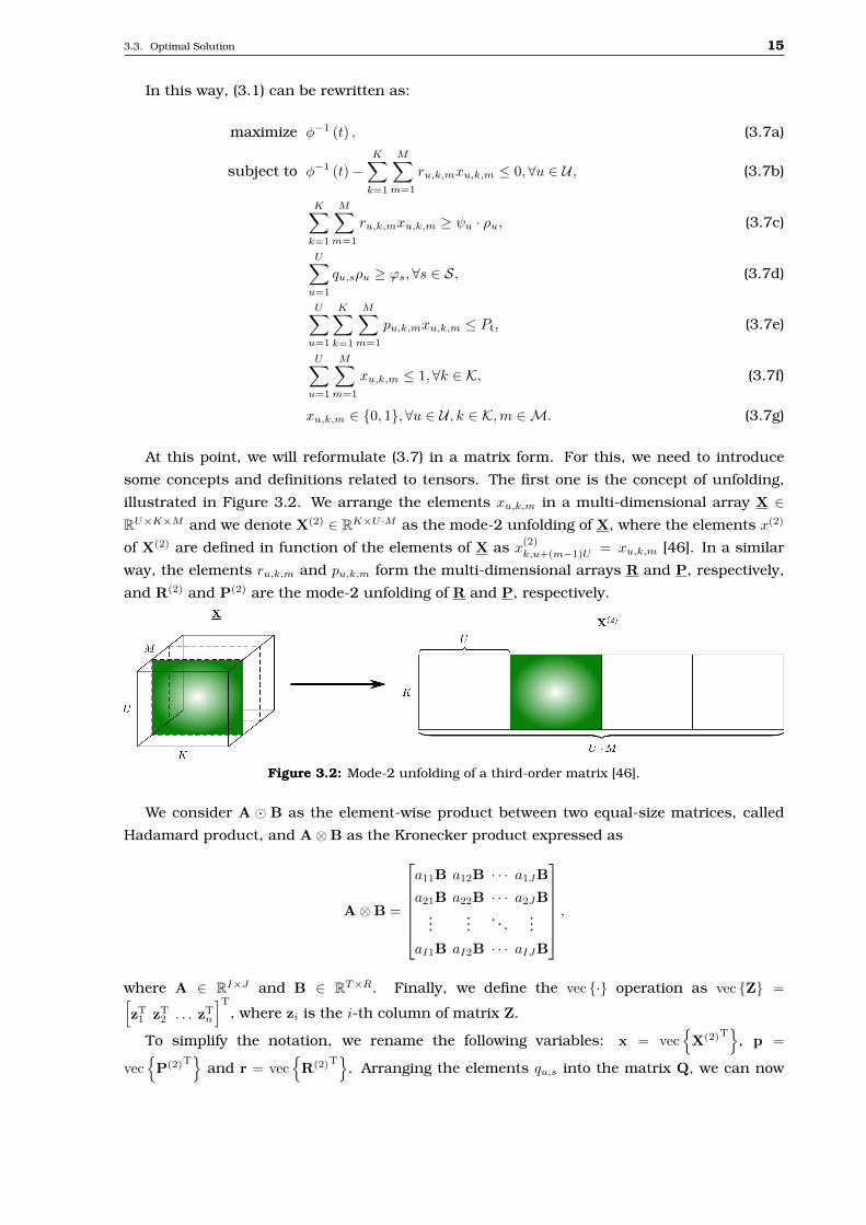
illustrated in Figure 3.2. We arrange the elements xu,k,m in a multi-dimensional array X ∈RU×K×M and we denote X(2) ∈ RK×U ·M as the mode-2 unfolding of X, where the elements x(2)
of X(2) are defined in function of the elements of X as x(2)k,u+(m−1)U = xu,k,m [46]. In a similar
way, the elements ru,k,m and pu,k,m form the multi-dimensional arrays R and P, respectively,
and R(2) and P(2) are the mode-2 unfolding of R and P, respectively.
Figure 3.2: Mode-2 unfolding of a third-order matrix [46].
We consider A � B as the element-wise product between two equal-size matrices, called
Hadamard product, and A⊗B as the Kronecker product expressed as
A⊗B =
a11B a12B · · · a1JB
a21B a22B · · · a2JB...
.... . .
...
aI1B aI2B · · · aIJB
,
where A ∈ RI×J and B ∈ RT×R. Finally, we define the vec {·} operation as vec {Z} =[zT1 zT2 . . . zTn
]T, where zi is the i-th column of matrix Z.
To simplify the notation, we rename the following variables: x = vec{
X(2)T}
, p =
vec{
P(2)T}
and r = vec{
R(2)T}
. Arranging the elements qu,s into the matrix Q, we can now
3.3. Optimal Solution 16
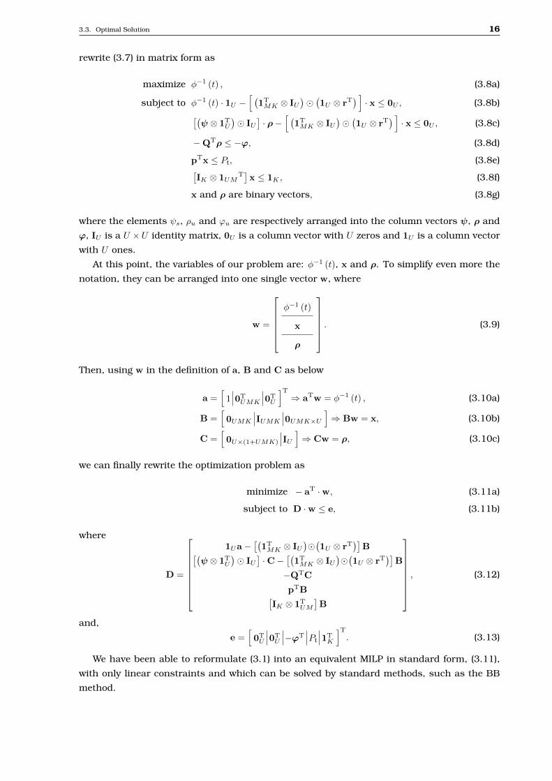
rewrite (3.7) in matrix form as
maximize φ−1 (t) , (3.8a)
subject to φ−1 (t) · 1U −[ (
1TMK ⊗ IU
)�(1U ⊗ rT
) ]· x ≤ 0U , (3.8b)[(
ψ ⊗ 1TU
)� IU
]· ρ−
[ (1TMK ⊗ IU
)�(1U ⊗ rT
) ]· x ≤ 0U , (3.8c)
−QTρ ≤ −ϕ, (3.8d)
pTx ≤ Pt, (3.8e)[IK ⊗ 1UM
T]x ≤ 1K , (3.8f)
x and ρ are binary vectors, (3.8g)
where the elements ψs, ρu and ϕu are respectively arranged into the column vectors ψ, ρ and
ϕ, IU is a U ×U identity matrix, 0U is a column vector with U zeros and 1U is a column vector
with U ones.
At this point, the variables of our problem are: φ−1 (t), x and ρ. To simplify even more the
notation, they can be arranged into one single vector w, where
w =
φ−1 (t)
x
ρ
. (3.9)
Then, using w in the definition of a, B and C as below
a =[1 0T
UMK 0TU
]T⇒ aTw = φ−1 (t) , (3.10a)
B =[
0UMK IUMK 0UMK×U
]⇒ Bw = x, (3.10b)
C =[
0U×(1+UMK) IU
]⇒ Cw = ρ, (3.10c)
we can finally rewrite the optimization problem as
minimize − aT ·w, (3.11a)
subject to D ·w ≤ e, (3.11b)
where
D =
1Ua−[(
1TMK ⊗ IU
)�(1U ⊗ rT
)]B[(
ψ ⊗ 1TU
)� IU
]·C−
[(1TMK ⊗ IU
)�(1U ⊗ rT
)]B
−QTC
pTB[IK ⊗ 1T
UM
]B
, (3.12)
and,
e =[
0TU 0T
U −ϕT Pt 1TK
]T. (3.13)
We have been able to reformulate (3.1) into an equivalent MILP in standard form, (3.11),
with only linear constraints and which can be solved by standard methods, such as the BB
method.
3.4. Proposed Solution 17
3.4 Proposed Solution
For real time systems, the optimal solution presented in Section 3.3 can still be impractical,
since, depending on the problem dimensions, it can still require high computational effort.
Motivated by this, in this section we develop a suboptimal heuristic solution, called Power and
Resource Allocation Based on Quality of Experience (PRABE), to solve (3.1) and to overcome
the complexity problem.
The proposed solution divides the problem (3.7) into two parts: the resource assignment
and the power allocation. In Section 3.4.1, we describe the resource assignment which is
performed considering Equal Power Allocation (EPA) among the RBs. In Section 3.4.2, we
describe the power allocation, which is done considering the previously performed resource
assignment.
3.4.1 Resource Allocation
Considering EPA among RBs, (3.7e) is always fulfilled (at most with equality) so that we
can rewrite problem (3.7) as
maximize φ−1 (t) (3.14a)
subject to φ−1 (t)−K∑
k=1
ru,kxu,k ≤ 0,∀u ∈ U , (3.14b)
K∑k=1
ru,kxu,k ≥ ψu · ρu,∀u ∈ U , (3.14c)
U∑u=1
qu,sρu ≥ ϕs,∀s ∈ S, (3.14d)
U∑u=1
xu,k ≤ 1,∀k, (3.14e)
xu,k and ρu ∈ {0, 1},∀u ∈ U and k ∈ K, (3.14f)
where xu,k is the binary assignment variable indicating whether the RB k is allocated to UE
u. Because the power per RB is constant, there is a single rate ru,k achievable by UE u
transmitting on an RB k, so that the total throughput Ru of UE u can be redefined as
Ru =
K∑k=1
ru,kxu,k. (3.15)
As done with (3.7), we can reformulate (3.14) into a matricial form. Arranging the
elements ru,k and xu,k in the matrices R and X, respectively, and denoting the Khatri-Rao
product for two matrices A =[a1 a2 · · · aJ
]∈ RI×J and B =
[b1 b2 · · · bJ
]∈ RT×J as
3.4. Proposed Solution 18
A ∗B =[a1 ⊗ b1 a2 ⊗ b2 · · · aJ ⊗ bJ
]we have
maximize φ−1 (t) , (3.16a)
subject to φ−1 (t) · 1U −(RT ∗ IU
)T· x ≤ 0U , (3.16b)[(
ψ ⊗ 1TU
)� IU
]· ρ−
(RT ∗ IU
)T· x ≤ 0U , (3.16c)
−QTρ ≤ −ϕ, (3.16d)[IK ⊗ 1U
T]x ≤ 1K , (3.16e)
x and ρ are binary vectors, (3.16f)
where x = vec{
X}
.
In order to collect the optimization variables in a single vector, we define
w =
φ−1 (t)
x
ρ
, (3.17)
so that
aT · w = φ−1 (t) with a =[1 0(UK+U)
T]T, (3.18a)
B · w = x with B = [0UK IUK 0UK×U ] , (3.18b)
and C · w = ρ with C =[0U×(1+UK) IU
]. (3.18c)
Finally, using (3.18), the optimization problem can be rewritten as
minimize − aT · w (3.19a)
subject to D · w ≤ e (3.19b)
where
D =
1U aT −
(RT ∗ IU
)TB[(
ψ ⊗ 1TU
)� IU
]· C−
(RT ∗ IU
)TB
−QTC[IK ⊗ 1T
U
]B
(3.20)
and,
e =[
0TU 0T
U −ϕ 1TK
]T. (3.21)
Problem (3.19) solves the resource assignment in an optimal way. Furthermore, compared
to (3.11), it has lower complexity since it solves the resource assignment considering EPA and,
thus, eliminating the power dimension of the optimization problem. However, its complexity
is still high for real time systems. Therefore, in order to obtain a suboptimal but efficient and
low-complexity solution to (3.19) we propose a new heuristic method presented in Figure 3.3.
Algorithm 3.1 presents, in algorithm form, how it can be implemented.
The flowchart in Fig. 3.3 is divided into two parts. On the first one we try to satisfy at least
ϕs UEs for each plan s, blocks (1) to (7). It is done in a loop, where in each step, an RB is
allocated to the UE that can achieve the highest transmit data rate on this RB. If this user
achieves the target MOS of his/her plan, he/she is removed from the set of users, block (3).
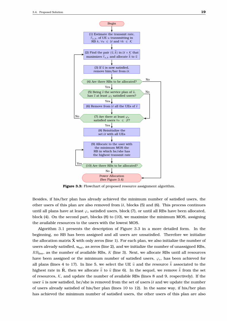
3.4. Proposed Solution 19
Begin
(1) Estimate the transmit rate,ru,k, of UE u transmitting inRB k, ∀u ∈ U and ∀k ∈ K
(2) Find the pair (u, k) in U × K thatmaximizes ru,k and allocate k to u
(3) If u is now satisfied,remove him/her from U .
(4) Are there RBs to be allocated?
(5) Being s the service plan of u,has s at least ϕs satisfied users?
(6) Remove from U all the UEs of s
(7) Are there at least ϕs
satisfied users ∀s ∈ S?
(8) Reinitialize theset U with all UEs
(9) Allocate to the user withthe minimum MOS the
RB in which he/she hasthe highest transmit rate
(10) Are there RBs to be allocated?
Power Allocation(See Figure 3.4)
No
Yes
Yes
No
No
Yes
Yes
No
Figure 3.3: Flowchart of proposed resource assignment algorithm.
Besides, if his/her plan has already achieved the minimum number of satisfied users, the
other users of this plan are also removed from U , blocks (5) and (6). This process continues
until all plans have at least ϕs satisfied users, block (7), or until all RBs have been allocated,
block (4). On the second part, blocks (8) to (10), we maximize the minimum MOS, assigning
the available resources to the users with the lowest MOS.
Algorithm 3.1 presents the description of Figure 3.3 in a more detailed form. In the
beginning, no RB has been assigned and all users are unsatisfied. Therefore we initialize
the allocation matrix X with only zeros (line 1). For each plan, we also initialize the number of
users already satisfied, usat, as zeros (line 2), and we initialize the number of unassigned RBs,
RBfree, as the number of available RBs, K (line 3). Next, we allocate RBs until all resources
have been assigned or the minimum number of satisfied users, ϕs, has been achieved for
all plans (lines 4 to 17). In line 5, we select the UE u and the resource k associated to the
highest rate in R, then we allocate k to u (line 6). In the sequel, we remove k from the set
of resources, K, and update the number of available RBs (lines 8 and 9, respectively). If the
user u is now satisfied, he/she is removed from the set of users U and we update the number
of users already satisfied of his/her plan (lines 10 to 12). In the same way, if his/her plan
has achieved the minimum number of satisfied users, the other users of this plan are also
3.4. Proposed Solution 20
removed. In line 18, we have three possibilities: the number of satisfied users has already
been achieved by all plan, all resources have been assigned or both. If there are still available
resources (in lines 18 to 28), they will be allocated aiming to maximize the minimum MOS.
First we identify, among all users, the one with the lowest MOS (line 21). Next, we chose
for him/her the remaining RB which maximizes his/her transmit data rate (line 22). This
algorithm finishes after the last available resource has been allocated.
Algorithm 3.1 Resource Allocation considering EPA.
1: X ← 0U×K . Initialize the allocation matrix2: usat ← 0S . For each plan, initialize the number of users already satisfied3: RBfree ← K . Initialize the number of unassigned RBs4: while (RBfree > 0 & usat < ϕ) do5: (u, k)← argmaxu∈U,k∈K ru,k6: x
u,k← 1 . Assign RB k to user u
7: Update τu8: K ← K \ {k} . Remove RB k from K9: RBfree ← RBfree − 1 . Update RBfree10: if τu ≥ φ (ψu) then . Test if user u is satisfied11: U ← U \ {u} . Remove user u from U12: usat (s) ← usat (s) + 1 . Update usat (s), where u ∈ Us13: if usat (s) ≥ ϕs then14: U ← U \ Us . Remove of U the UEs of s15: end if16: end if17: end while18: if RBfree > 0 then19: Reinitialize the set U with all users20: while (RBfree > 0) do21: u← argminu∈U τu . Find the user with the lowest MOS22: k ← argmaxk∈K ru,k23: x
u,k← 1 . Assign RB k to user u
24: Update τu25: K ← K \ {k} . Remove RB k from K26: RBfree ← RBfree − 1 . Update RBfree27: end while28: end if
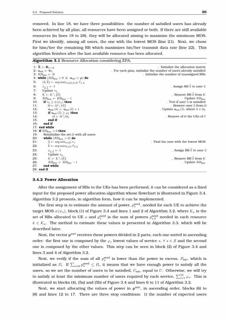
3.4.2 Power Allocation
After the assignment of RBs to the UEs has been performed, it can be considered as a fixed
input for the proposed power allocation algorithm whose flowchart is illustrated in Figure 3.4.
Algorithm 3.2 presents, in algorithm form, how it can be implemented.
The first step is to estimate the amount of power, pneedu , needed for each UE to achieve the
target MOS φ (ψu), block (1) of Figure 3.4 and lines 1 and 2 of Algorithm 3.2, where Ku is the
set of RBs allocated to UE u and pneedu is the sum of powers pneed
u,k needed in each resource
k ∈ Ku. The method to estimate these values is presented in Algorithm 3.3, which will be
described later.
Next, the vector psort receives these powers divided in 2 parts, each one sorted in ascending
order: the first one is composed by the ϕs lowest values of service s, ∀ s ∈ S and the second
one is composed by the other values. This step can be seen in block (2) of Figure 3.4 and
lines 3 and 4 of Algorithm 3.2.
Next, we verify if the sum of all pneedu is lower than the power in excess, Pexc, which is
initialized as Pt. If∑
u∈U pneedu ≤ Pt, it means that we have enough power to satisfy all the
users, so we set the number of users to be satisfied, Usat, equal to U . Otherwise, we will try
to satisfy at least the minimum number of users required by each service,∑|S|
s=1 ϕs. This is
illustrated in blocks (4), (5a) and (5b) of Figure 3.4 and lines 6 to 11 of Algorithm 3.2.
Next, we start allocating the values of power in psort, in ascending order, blocks (6) to
(8) and lines 12 to 17. There are three stop conditions: 1) the number of expected users
3.4. Proposed Solution 21
Resource Allocation (EPA)(See Figure 3.3)
(1) Estimate the power needed,pneedu =
∑∀k∈Ku
pneedu,k , to each UE u,
targeting the threshold MOS φ (ψu)(See Figure 3.5)
(2) Vector psort receives thesepowers divided in 2 parts, eachone sorted in ascending order:
- The first one is composedby the ϕs lowest values
of service s, ∀ s ∈ S- The second one is
composed by the other values
(3) Set Pexc = Pt and i = 1
(4) Is the sum of thesepowers lower or equal to
the power in excess, Pexc?
(5a) Set thenumber of usersto be satisfied,Usat, equal to the
number of users, U
(5b) Set Usat equalto the minimum
number of satisfiedusers,
∑|S|s=1 ϕs
(6) The user corresponding to psorti ,
the ith entry of psort, receives psorti
(7) Update Pexc; Incrementi; Decrement Usat
(8) Is Usat = 0 orPexc = 0 or psort
i > Pexc?
(9) Now, we have l levels of MOS,where l ≤ s + 1 and θj is thej − th lowest value. Initialize,j = 1 and set θl+1 = 5.
(10) Distribute Pexc among theUEs with MOS θj , aiming toequally increase their MOS
until achieving at maximum θj+1
(See Figure 3.6)
(11) Increment j and update Pexc
(12) Is Pexc > 0 and j < l + 1?
End
Yes No
Yes
No
Yes
No
Figure 3.4: Flowchart of proposed power allocation algorithm.
to be satisfied, Usat =∑|S|
s=1 ϕs, has been achieved, 2) there is a lack of in-excess power to be
allocated or 3) the next value of power, pneedu , to be allocated is higher than the excess of power.
At this point, we have l levels of MOS, with 1 ≤ l ≤ s + 1, where l = 1 if all UEs have MOS
3.4. Proposed Solution 22
Algorithm 3.2 Power allocation.
1: ∀u ∈ U , call Algorithm 3.3 to estimate pneedu,k , ∀k ∈ Ku, aiming MOS φ (ψu)
2: ∀u ∈ U , pneedu ←∑
∀k∈Kupneedu,k
3: ∀u ∈ Us and ∀s ∈ S, ps ← sort(pneedu )
4: psort ← sort(⋃∀s∈S∀i∈[1,ϕs]
psi
)⋃sort
(⋃∀s∈S∀i∈[ϕs+1,Us]
psi
)5: i← 16: Pexc ← Pt7: if
∑u∈U p
needu ≤ Pexc then
8: Usat ← U . Satisfy all the users9: else10: Usat ←
∑|S|s=1 ϕs . Try to satisfy at least the minimum number of users required for each service
11: end if12: while
(Usat > 0 & Pexc > 0 & psort
i ≤ Pexc)
do13: pi,k ← psort
i,k , ∀k ∈ Ki . Power allocation of user i14: Pexc ← Pexc −
∑∀k∈Ki
psorti,k . Update Pexc
15: Usat ← Usat − 1 . User i is satisfied, so decrease Usat16: i← i+ 1 . Increment i17: end while18: θ ← unique(sort(τ )) . θj is the j − th lowest MOS19: θl+1 ← 5 . 5 is the highest MOS that can be achieved20: j ← 121: while Pexc > 0 & j < l+ 1 do22: Call Algorithm 3.4 to distribute Pexc among the UEs with MOS θj aiming at maximum the MOS θj+1
23: j ← j + 124: end while
equal to zero and l = s + 1 if at least one UE of each service has achieved the target MOS of
its service and there are still some UE with MOS equal to zero. These l levels are arranged in
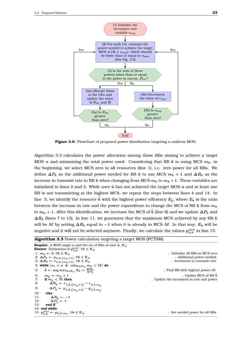
ascending order in θ, where θj is the j-th lowest value and θl+1 = 5 is the highest MOS that
can be achieved, block (7) and lines 18 and 19.
Finally, in steps (9) to (12) and lines 21 to 23, for each level of MOS we will distribute
Pexc among the UEs of this level aiming to achieve the next level of MOS. If there is still Pexc
these UEs will joint the UEs of the next level and the power distribution will be repeated. The
algorithm to distribute the in-excess power among a set of users in a way that all achieve the
same MOS is presented in Algorithm 3.4.
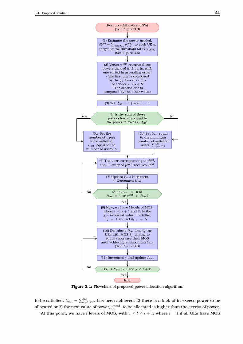
It is also worthy to mention that Algorithms 3.3 and 3.4 are based on Hughes-Hartogs
Bit-Loading Algorithm [47]. Given a specific UE u and the set of RBs allocated to it, Ku,
(1) Initialize all RBsof a specific UEin Modulationand Coding
Scheme (MCS) zero
(2) Estimate the power efficiency ofeach RB, i.e., the ratio between theincrease in rate and the expense inpower when increasing their MCS
(3) - Increase the MCS of the RBwith the highest power efficiency
- Allocate to it the necessary powerto transmit using this new MCS- Estimate its power efficiency
(4) Is the user’s MOS equal to orhigher than n or is his/her lowestMCS equal to or higher than M?
End
Yes
No
Figure 3.5: Flowchart of proposed power calculation to achieve a target MOS for a specific user.
3.4. Proposed Solution 23
(1) Initialize theincrement ratevariable rstep
(2) For each UE, estimate thepower needed to achieve the targetMOS φ (R+ rstep), which should
be lower than or equal to nmax(See Fig. 3.5)
(3) Is the sum of thesepowers lower than or equal
to the power in excess, Pexc?
(4a) Allocate themto the UEs and
update the valueof Pexc and R
(4b) Decrementthe value of rstep
(5a) Is Pexcgreater
than zero?
(5b) Is rstepgreater
than zero?
End
Yes No
NoNo
Yes Yes
Figure 3.6: Flowchart of proposed power distribution targeting a uniform MOS.
Algorithm 3.3 calculates the power allocation among these RBs aiming to achieve a target
MOS n and minimizing the total power used. Considering that RB k is using MCS mk, in
the beginning, we select MCS zero to all resources (line 1), i.e. zero power for all RBs. We
define ∆Pk as the additional power needed for RB k to use MCS mk + 1 and ∆Rk as the
increase in transmit rate in RB k when changing from MCS mk to mk +1. These variables are
initialized in lines 2 and 3. While user u has not achieved the target MOS n and at least one
RB is not transmitting at the highest MCS, we repeat the steps between lines 4 and 14. In
line 5, we identify the resource k with the highest power efficiency Ek, where Ek is the ratio
between the increase in rate and the power expenditure to change the MCS of RB k from mk
to mk + 1. After this identification, we increase the MCS of k (line 6) and we update ∆Pk and
∆Rk (lines 7 to 13). In line 11, we guarantee that the maximum MCS achieved by any RB k
will be M by setting ∆Rk equal to −1 when it is already in MCS M . In that way, Ek will be
negative and it will not be selected anymore. Finally, we calculate the values pneedu,k in line 15.
Algorithm 3.3 Power calculation targeting a target MOS (PCTSM).Require: A MOS target n and the set of RBs of user u, Ku
Ensure: Estimation of pneedu,k
, ∀k ∈ Ku
1: mk ← 0, ∀k ∈ Ku . Initialize all RBs in MCS zero2: ∆Pk ← pu,k,(mk+1), ∀k ∈ Ku . Additional power needed3: ∆Rk ← ru,k,(mk+1), ∀k ∈ Ku . Increment in transmit rate4: while
(τu < n & mink∈Ku
mk < M)
do5: k← arg maxk∈Ku
Ek = ∆Rk∆Pk
. Find RB with highest power eff.
6: mk← m
k+ 1 . Update MCS of RB k
7: if mk< M then . Update the increment in rate and power
8: ∆Rk← r
u,k,(mk+1) − ru,k,m
k
9: ∆Pk← p
u,k,(mk+1) − pu,k,m
k
10: else11: ∆R
k← −1
12: ∆Pk← 1
13: end if14: end while15: pneed
u,k← pu,k,mk
, ∀k ∈ Ku . Set needed power for all RBs
3.5. Partial Conclusions 24
Algorithm 3.4 Power distribution targeting a uniform MOS (PDTUM).Require: A set of UEs U ′, their RBs, an excess of power, Pexc, and an upper bound nmax1: Initialize rstep2: while Pexc > 0 & φ (R+ rstep) ≤ nmax do3: ∀u ∈ U ′, call Alg.3.3 to estimate pneed
u,k , ∀k ∈ Ku, aiming φ (R+ rstep)
4: pneedu,k ← PCTSM (φ (R+ rstep)), ∀u ∈ U ′
5: if pu,k = pneedu,k , ∀u ∈ U ′, k ∈ Ku then
6: Stop7: end if8: if
∑∀u∈U′
∑∀k∈Ku
(pneedu − pu
)≤ Pexc then
9: pu,k ← pneedu,k , ∀u ∈ U ′, k ∈ Ku
10: Pexc ← Pexc −∑
∀u∈U′∑
∀k∈Ku
(pneedu,k − pu,k
)11: R← R+ rstep12: else13: Decrement rstep14: if rstep = 0 then15: Distribute Pexc in ascending order of
∑∀k∈Ku
pneedu
16: end if17: end if18: end while
Given an amount of power Pexc and a set of users, U ′, in which all users have
approximatively the same transmit rate R and so approximatively the same MOS φ(R),
Algorithm 3.4 allocates Pexc among these users and their RBs, in a way that all users increase
their MOS equally. It works as follow: 1) We fix a target value of rate R + rstep, where
φ(R+ rstep
)must be lower than or equal to an upper bound nmax, and, in line 4, we use
Algorithm 3.3, to estimate the needed power for all UEs to transmit using the rate R + rstep;
2) If the increase in power that we need to have to achieve this purpose is lower than or equal
to Pexc, in lines 8 to 11, we distribute the power and update the value of R; 3) Otherwise, we
decrement the value of rstep and try again. In case rstep becomes zero, we stop. The initial
value of rstep and the way it will decrement is chosen by the operator. This choice has an
important impact on the algorithm complexity.
3.5 Partial Conclusions
In this chapter, we presented a radio resource assignment problem aiming at maximizing
the minimum MOS of the system subject to attaining at least a minimum number of satisfied
users. It was initially formulated as a non-linear problem, but we managed to reformulate
it as a MILP, solvable by standard methods, as the BB. Finally, we presented our proposal,
consisting of two parts. The first one assigns the resources considering EPA, while the second
one allocates power considering the previous resource allocation. In the next chapter, we
evaluate our proposal, by means of simulations, comparing it with the optimal solution, as
well as with two benchmarking algorithms and with a mixed solution, which uses as resource
assignment the optimal solution of (3.19) and as power allocation the heuristic proposed in
Algorithm 3.2, Section 3.4.2.
Chapter 4Performance Evaluation
4.1 Introduction
In this chapter, we evaluate the proposed Power and Resource Allocation Based on
Quality of Experience (PRABE) algorithm and compare its performance with that of the
optimal solution, of a mixed-solution, as well as with that of two benchmarking algorithms.
In Section 4.2, we present the simulation parameters, the benchmarking algorithms, the
evaluated scenarios and the evaluation metrics. In Section 4.3, we present the results and
the discussions.
4.2 Simulation Assumptions
The system model configuration presented in Chapter 2 was adopted for all simulations.
The system parameters were aligned with the 3rd Generation Partnership Project (3GPP) Long
Term Evolution (LTE) architecture.
A hexagonal cell with 1 km radius was considered, within which there was one Evolved
Node B (eNB) with a three-sectored antenna. We adopted a system bandwidth of 5 MHz
and carrier frequency of 2 GHz. The system disposed of 25 Resource Blocks (RBs), each
one consisting of 12 adjacent subcarriers. The propagation effects on the wireless channel
included a lognormal shadowing component and a distance-dependent path-loss, as well as
small-scale fading. We also adopted a 3D antenna model, as in [48], considering a downtilt
angle in order to increase cell isolation and to mitigate the effects of inter-cell interference.
Table 4.1 presents the main adopted parameters. In subsections 4.3.1, 4.3.2 and 4.3.4 we
consider path loss model 1 and in subsection 4.3.3 we consider path loss model 2.
The Mean Opinion Score (MOS) function, φ (·), adopted for the simulations is proposed
in [53]. It is an utility function for web connections in LTE, in accordance with the scenario
adopted in this master’s thesis. It is presented in (4.1) and illustrated in Figure 4.1.
φ(Ru) = 5−578
1 +
(Ru + 541.1
45.98
)2 , (4.1)
where Ru is the total throughput of UE u.
Four different scenarios were adopted to evaluate the performance of the proposed
algorithm:
I The first one considered only one service plan. We analyzed the impact of the target
MOS for different numbers of UEs in the system, as well as the impact of the satisfaction
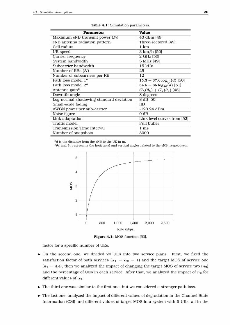
4.2. Simulation Assumptions 26
Table 4.1: Simulation parameters.
Parameter ValueMaximum eNB transmit power (Pt) 43 dBm [49]eNB antenna radiation pattern Three-sectored [49]Cell radius 1 kmUE speed 3 km/h [50]Carrier frequency 2 GHz [50]System bandwidth 5 MHz [49]Subcarrier bandwidth 15 kHzNumber of RBs (K) 25Number of subcarriers per RB 12Path loss model 1a 15.3 + 37.6 log10(d) [50]Path loss model 2a 34.5 + 35 log10(d) [51]Antenna gainb Gh(θh) +Gv(θv) [48]Downtilt angle 8 degreesLog-normal shadowing standard deviation 8 dB [50]Small-scale fading IIDAWGN power per sub-carrier -123.24 dBmNoise figure 9 dBLink adaptation Link level curves from [52]Traffic model Full bufferTransmission Time Interval 1 msNumber of snapshots 3000
ad is the distance from the eNB to the UE in m.bθh and θv represents the horizontal and vertical angles related to the eNB, respectively.
0 500 1,000 1,500 2,000 2,500
1
2
3
4
5
Rate (kbps)
MO
S
Figure 4.1: MOS function [53].
factor for a specific number of UEs.
I On the second one, we divided 20 UEs into two service plans. First, we fixed the
satisfaction factor of both services (α1 = α2 = 1) and the target MOS of service one
(n1 = 4.4), then we analyzed the impact of changing the target MOS of service two (n2)
and the percentage of UEs in each service. After that, we analyzed the impact of n2 for
different values of α2.
I The third one was similar to the first one, but we considered a stronger path loss.
I The last one, analyzed the impact of different values of degradation in the Channel State
Information (CSI) and different values of target MOS in a system with 5 UEs, all in the
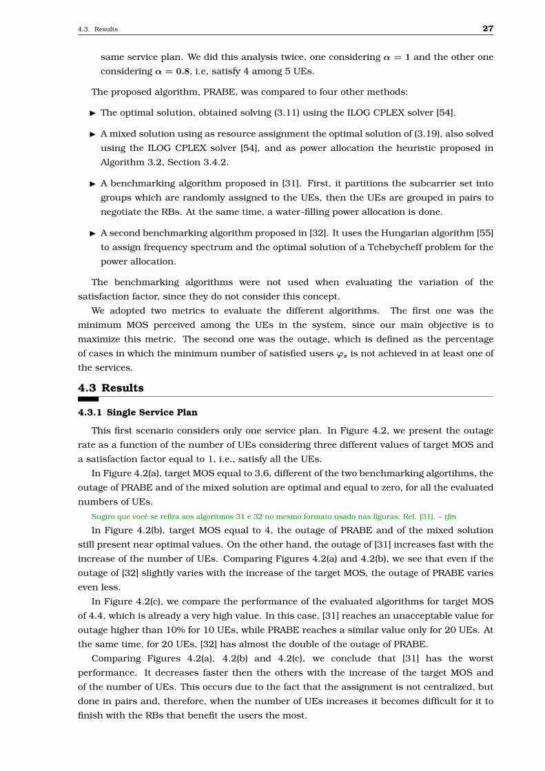
4.3. Results 27
same service plan. We did this analysis twice, one considering α = 1 and the other one
considering α = 0.8, i.e, satisfy 4 among 5 UEs.
The proposed algorithm, PRABE, was compared to four other methods:
I The optimal solution, obtained solving (3.11) using the ILOG CPLEX solver [54].
I A mixed solution using as resource assignment the optimal solution of (3.19), also solved
using the ILOG CPLEX solver [54], and as power allocation the heuristic proposed in
Algorithm 3.2, Section 3.4.2.
I A benchmarking algorithm proposed in [31]. First, it partitions the subcarrier set into
groups which are randomly assigned to the UEs, then the UEs are grouped in pairs to
negotiate the RBs. At the same time, a water-filling power allocation is done.
I A second benchmarking algorithm proposed in [32]. It uses the Hungarian algorithm [55]
to assign frequency spectrum and the optimal solution of a Tchebycheff problem for the
power allocation.
The benchmarking algorithms were not used when evaluating the variation of the
satisfaction factor, since they do not consider this concept.
We adopted two metrics to evaluate the different algorithms. The first one was the
minimum MOS perceived among the UEs in the system, since our main objective is to
maximize this metric. The second one was the outage, which is defined as the percentage
of cases in which the minimum number of satisfied users ϕs is not achieved in at least one of
the services.
4.3 Results
4.3.1 Single Service Plan
This first scenario considers only one service plan. In Figure 4.2, we present the outage
rate as a function of the number of UEs considering three different values of target MOS and
a satisfaction factor equal to 1, i.e., satisfy all the UEs.
In Figure 4.2(a), target MOS equal to 3.6, different of the two benchmarking algortihms, the
outage of PRABE and of the mixed solution are optimal and equal to zero, for all the evaluated
numbers of UEs.
Sugiro que você se refira aos algoritmos 31 e 32 no mesmo formato usado nas figuras: Ref. [31]. – tfm
In Figure 4.2(b), target MOS equal to 4, the outage of PRABE and of the mixed solution
still present near optimal values. On the other hand, the outage of [31] increases fast with the
increase of the number of UEs. Comparing Figures 4.2(a) and 4.2(b), we see that even if the
outage of [32] slightly varies with the increase of the target MOS, the outage of PRABE varies
even less.
In Figure 4.2(c), we compare the performance of the evaluated algorithms for target MOS
of 4.4, which is already a very high value. In this case, [31] reaches an unacceptable value for
outage higher than 10% for 10 UEs, while PRABE reaches a similar value only for 20 UEs. At
the same time, for 20 UEs, [32] has almost the double of the outage of PRABE.
Comparing Figures 4.2(a), 4.2(b) and 4.2(c), we conclude that [31] has the worst
performance. It decreases faster then the others with the increase of the target MOS and
of the number of UEs. This occurs due to the fact that the assignment is not centralized, but
done in pairs and, therefore, when the number of UEs increases it becomes difficult for it to
finish with the RBs that benefit the users the most.
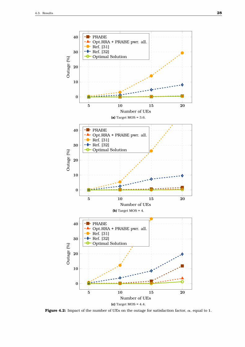
4.3. Results 28
5 10 15 20
0
10
20
30
40
Number of UEs
Ou
tage
(%)
PRABEOpt.RRA + PRABE pwr. all.Ref. [31]Ref. [32]Optimal Solution
(a) Target MOS = 3.6.
5 10 15 20
0
10
20
30
40
Number of UEs
Ou
tage
(%)
PRABEOpt.RRA + PRABE pwr. all.Ref. [31]Ref. [32]Optimal Solution
(b) Target MOS = 4.
5 10 15 20
0
10
20
30
40
Number of UEs
Ou
tage
(%)
PRABEOpt.RRA + PRABE pwr. all.Ref. [31]Ref. [32]Optimal Solution
(c) Target MOS = 4.4.
Figure 4.2: Impact of the number of UEs on the outage for satisfaction factor, α, equal to 1.
4.3. Results 29
The analyses of the minimum MOS versus the number of UEs are presented in Figure 4.3,
considering the same setup of the outage analyses, Figure 4.2. In order to perform a fair
comparison, we consider only the cases where the optimal solution is feasible.
In Figure 4.3(a), target MOS equal to 3.6, we notice that the performance of PRABE and
of the mixed solution is almost indistinguishable of the optimal one. We also identify a
considerable gap between PRABE and [31]. For 20 UEs, the minimum MOS of [31] does
not even reach the target MOS, 3.6.
In Figure 4.3(b), target MOS equal to 4, we notice that PRABE still has a near optimal
performance. Its minimum MOS still reaches values higher than the target MOS for all the
number of UEs, while [31] does not achieve this value when we have more than 15 UEs. In
this case, the algorithm of [32] is better than [31] but still worse than PRABE.
Comparing Figures 4.3(a) and 4.3(b), we notice that, for the same number of UEs, when
the target MOS changes from 3.6 to 4, the gap between the minimum MOS of [31] and [32]
decreases due to the enhancement of [31]. However, the difference between PRABE and the
benchmarking algorithms is still considerable.
In Figure 4.3(c), target MOS 4.4, PRABE still has a near optimal behavior, differing from
the optimal solution only when we have 20 UEs in the system. Different of the benchmarking
algorithms, only in this case, the minimum MOS is lower than the target MOS, indicating
cases of outage.
It is important to note in Figures 4.2 and 4.3 that the proposed algorithm, PRABE, performs
very close to the optimal solution, deviating from it only when the target MOS becomes high
and the number of UEs becomes close to the number of RBs. Nevertheless, the performance of
the proposed algorithm is still considerably better than those of the benchmarking algorithms.
One way of increasing the performace of PRABE, for high values of target MOS and UEs
in the system, is reducing the satisfaction factor. Figure 4.4 presents the outage versus the
satisfaction factor, in percentage, in a system with 20 UEs and target MOS equal to 4.4. This
analysis does not consider the benchmarking algorithms, [31] and [32], since they were not
designed to support a satisfaction factor lower than 1. However, this parameter plays an
important role, especially for network operators, since it is not always possible to satisfy all
UEs at the same time in real-life networks. As we can observe in Figure 4.4, just by changing
this parameter from 100% (satisfy 20 users out of 20) to 95% (satisfy 19 users out of 20) is
enough to obtain an acceptable value of outage.
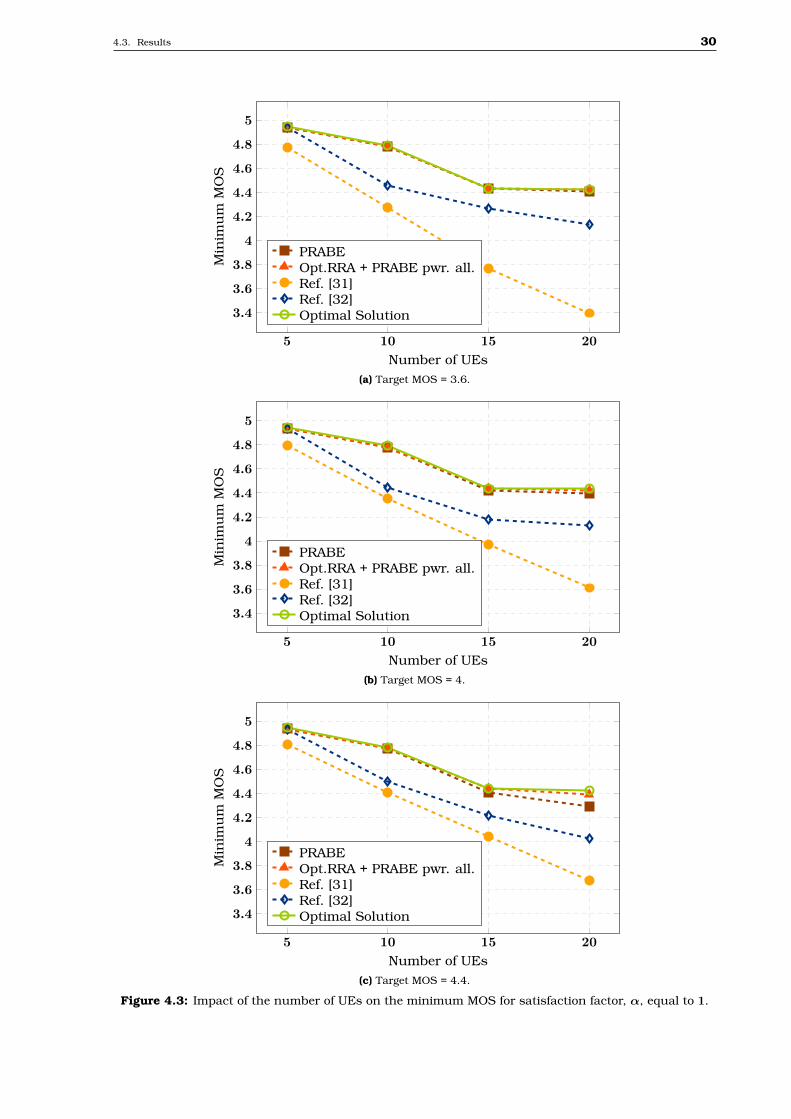
4.3. Results 30
5 10 15 20
3.4
3.6
3.8
4
4.2
4.4
4.6
4.8
5
Number of UEs
Min
imu
mM
OS
PRABEOpt.RRA + PRABE pwr. all.Ref. [31]Ref. [32]Optimal Solution
(a) Target MOS = 3.6.
5 10 15 20
3.4
3.6
3.8
4
4.2
4.4
4.6
4.8
5
Number of UEs
Min
imu
mM
OS
PRABEOpt.RRA + PRABE pwr. all.Ref. [31]Ref. [32]Optimal Solution
(b) Target MOS = 4.
5 10 15 20
3.4
3.6
3.8
4
4.2
4.4
4.6
4.8
5
Number of UEs
Min
imu
mM
OS
PRABEOpt.RRA + PRABE pwr. all.Ref. [31]Ref. [32]Optimal Solution
(c) Target MOS = 4.4.
Figure 4.3: Impact of the number of UEs on the minimum MOS for satisfaction factor, α, equal to 1.
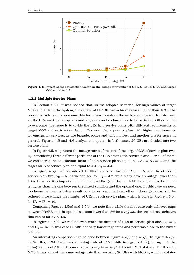
4.3. Results 31
80 85 90 95 100
0
5
10
Satisfaction Percentage (%)
Ou
tage
(%)
PRABEOpt.RRA + PRABE pwr. all.Optimal Solution
Figure 4.4: Impact of the satisfaction factor on the outage for number of UEs, U , equal to 20 and targetMOS equal to 4.4.
4.3.2 Multiple Service Plans
In Section 4.3.1, it was noticed that, in the adopted scenario, for high values of target
MOS and UEs in the system, the outage of PRABE can achieve values higher than 10%. The
presented solution to overcome this issue was to reduce the satisfaction factor. In this case,
all the UEs are treated equally and any one can be chosen not to be satisfied. Other option
to overcome this issue is to divide the UEs into service plans with different requirements of
target MOS and satisfaction factor. For example, a priority plan with higher requirements
for emergency services, as fire brigade, police and ambulances, and another one for users in
general. Figures 4.5 and 4.6 analyze this option. In both cases, 20 UEs are divided into two
service plans.
In Figure 4.5, we present the outage rate as function of the target MOS of service plan two,
n2, considering three different partitions of the UEs among the service plans. For all of them,
we considered the satisfaction factor of both service plans equal to 1, α1 = α2 = 1, and the
target MOS of service plan one equal to 4.4, n1 = 4.4.
In Figure 4.5(a), we considered 15 UEs in service plan one, U1 = 15, and the others in
service plan two, U2 = 5. As we can see, for n2 = 4.2, we already have an outage lower than
10%. However, it is important to mention that the gap between PRABE and the mixed solution
is higher than the one between the mixed solution and the optimal one. In this case we need
to choose between a better result or a lower computational effort. These gaps can still be
reduced if we change the number of UEs in each service plan, which is done in Figure 4.5(b),
for U1 = U2 = 10.
Comparing Figures 4.5(a) and 4.5(b), we note that, while the first case only achieves gaps
between PRABE and the optimal solution lower than 5% for n2 ≤ 3.6, the second case achieves
this values for n2 ≤ 4.2.
In Figures 4.5(c), we reduce even more the number of UEs in service plan one, U1 = 5
and U2 = 15. In this case PRABE has very low outage rates and performs close to the mixed
solution.
An interesting comparison can be done between Figure 4.2(b) and 4.5(c). In Figure 4.2(b),
for 20 UEs, PRABE achieves an outage rate of 1.7%, while in Figures 4.5(c), for n2 = 4, the
outage rate is of 2.6%. This means that trying to satisfy 5 UEs with MOS 4.4 and 15 UEs with
MOS 4, has almost the same outage rate than assuring 20 UEs with MOS 4, which validates
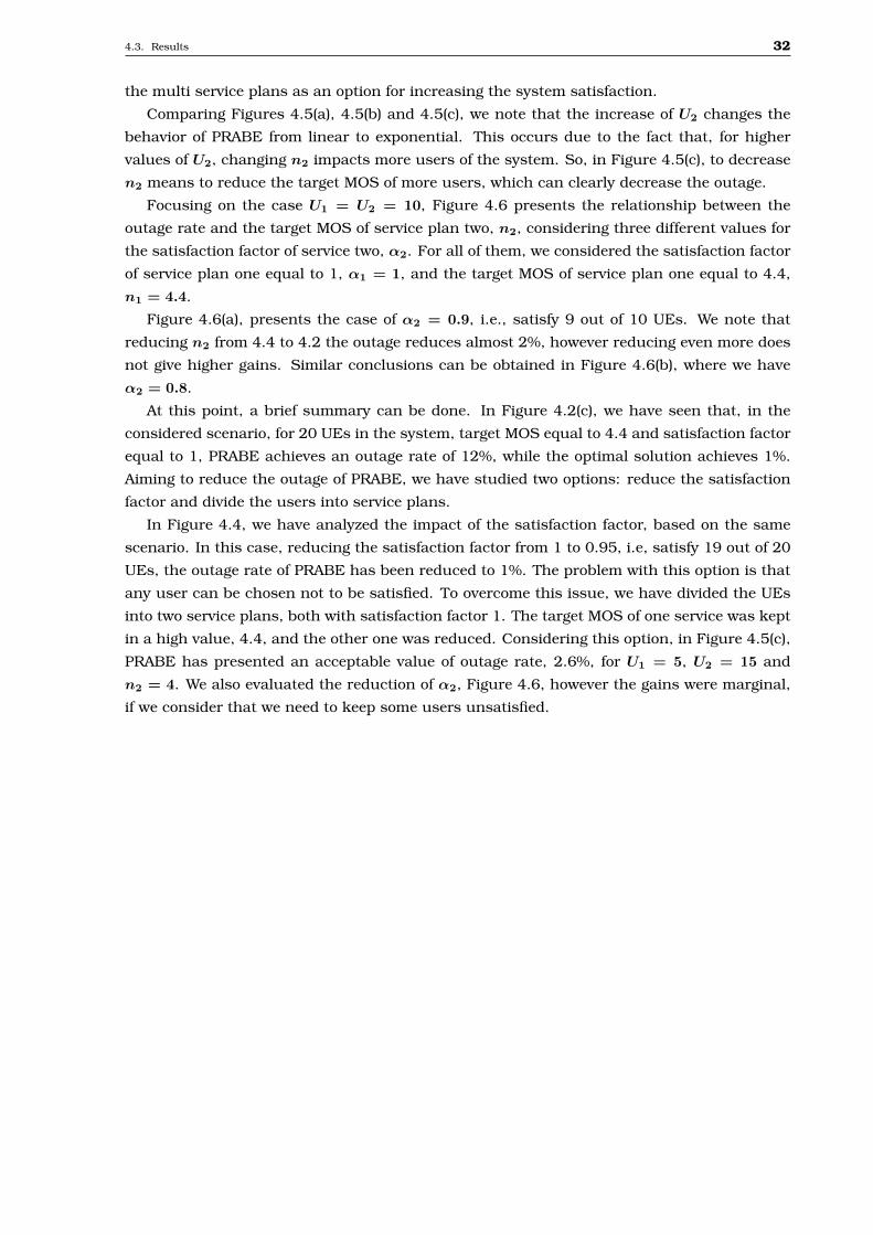
4.3. Results 32
the multi service plans as an option for increasing the system satisfaction.
Comparing Figures 4.5(a), 4.5(b) and 4.5(c), we note that the increase of U2 changes the
behavior of PRABE from linear to exponential. This occurs due to the fact that, for higher
values of U2, changing n2 impacts more users of the system. So, in Figure 4.5(c), to decrease
n2 means to reduce the target MOS of more users, which can clearly decrease the outage.
Focusing on the case U1 = U2 = 10, Figure 4.6 presents the relationship between the
outage rate and the target MOS of service plan two, n2, considering three different values for
the satisfaction factor of service two, α2. For all of them, we considered the satisfaction factor
of service plan one equal to 1, α1 = 1, and the target MOS of service plan one equal to 4.4,
n1 = 4.4.
Figure 4.6(a), presents the case of α2 = 0.9, i.e., satisfy 9 out of 10 UEs. We note that
reducing n2 from 4.4 to 4.2 the outage reduces almost 2%, however reducing even more does
not give higher gains. Similar conclusions can be obtained in Figure 4.6(b), where we have
α2 = 0.8.
At this point, a brief summary can be done. In Figure 4.2(c), we have seen that, in the
considered scenario, for 20 UEs in the system, target MOS equal to 4.4 and satisfaction factor
equal to 1, PRABE achieves an outage rate of 12%, while the optimal solution achieves 1%.
Aiming to reduce the outage of PRABE, we have studied two options: reduce the satisfaction
factor and divide the users into service plans.
In Figure 4.4, we have analyzed the impact of the satisfaction factor, based on the same
scenario. In this case, reducing the satisfaction factor from 1 to 0.95, i.e, satisfy 19 out of 20
UEs, the outage rate of PRABE has been reduced to 1%. The problem with this option is that
any user can be chosen not to be satisfied. To overcome this issue, we have divided the UEs
into two service plans, both with satisfaction factor 1. The target MOS of one service was kept
in a high value, 4.4, and the other one was reduced. Considering this option, in Figure 4.5(c),
PRABE has presented an acceptable value of outage rate, 2.6%, for U1 = 5, U2 = 15 and
n2 = 4. We also evaluated the reduction of α2, Figure 4.6, however the gains were marginal,
if we consider that we need to keep some users unsatisfied.
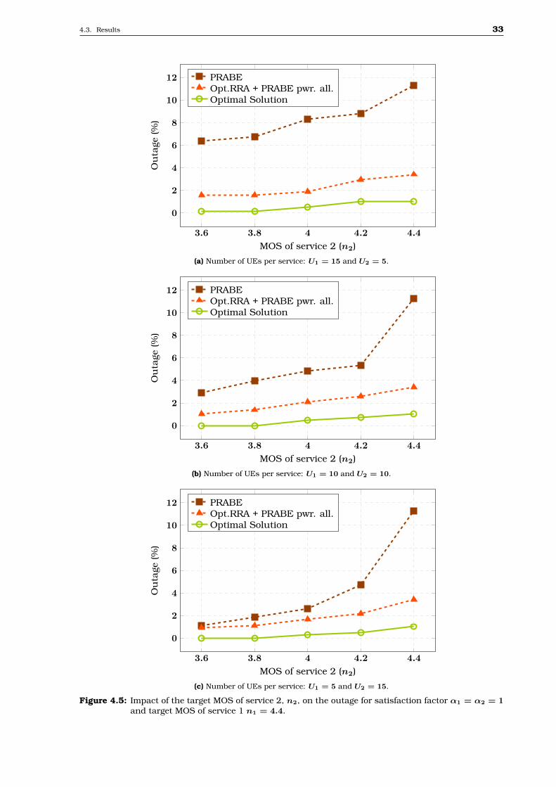
4.3. Results 33
3.6 3.8 4 4.2 4.4
0
2
4
6
8
10
12
MOS of service 2 (n2)
Ou
tage
(%)
PRABEOpt.RRA + PRABE pwr. all.Optimal Solution
(a) Number of UEs per service: U1 = 15 and U2 = 5.
3.6 3.8 4 4.2 4.4
0
2
4
6
8
10
12
MOS of service 2 (n2)
Ou
tage
(%)
PRABEOpt.RRA + PRABE pwr. all.Optimal Solution
(b) Number of UEs per service: U1 = 10 and U2 = 10.
3.6 3.8 4 4.2 4.4
0
2
4
6
8
10
12
MOS of service 2 (n2)
Ou
tage
(%)
PRABEOpt.RRA + PRABE pwr. all.Optimal Solution
(c) Number of UEs per service: U1 = 5 and U2 = 15.
Figure 4.5: Impact of the target MOS of service 2, n2, on the outage for satisfaction factor α1 = α2 = 1and target MOS of service 1 n1 = 4.4.
4.3. Results 34
3.6 3.8 4 4.2 4.4
0
1
2
3
4
MOS of service 2 (n2)
Ou
tage
(%)
PRABEOpt.RRA + PRABE pwr. all.Optimal Solution
(a) Satisfaction factor of service plan 2: α2 = 0.9.
3.6 3.8 4 4.2 4.4
0
1
2
3
4
MOS of service 2 (n2)
Ou
tage
(%)
PRABEOpt.RRA + PRABE pwr. all.Optimal Solution
(b) Satisfaction factor of service plan 2: α2 = 0.8.
Figure 4.6: Impact of the target MOS of service 2, n2, on the outage for 10 UEs in each service, U1 =U2 = 10, satisfaction factor α1 = 1 and target MOS of service 1 n1 = 4.4.
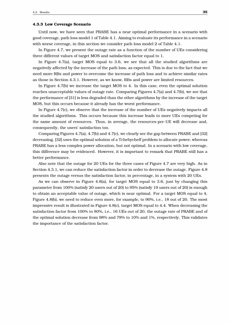
4.3. Results 35
4.3.3 Low Coverage Scenario
Until now, we have seen that PRABE has a near optimal performance in a scenario with
good coverage, path loss model 1 of Table 4.1. Aiming to evaluate its performance in a scenario
with worse coverage, in this section we consider path loss model 2 of Table 4.1.
In Figure 4.7, we present the outage rate as a function of the number of UEs considering
three different values of target MOS and satisfaction factor equal to 1.
In Figure 4.7(a), target MOS equal to 3.6, we see that all the studied algorithms are
negatively affected by the increase of the path loss, as expected. This is due to the fact that we
need more RBs and power to overcome the increase of path loss and to achieve similar rates
as those in Section 4.3.1. However, as we know, RBs and power are limited resources.
In Figure 4.7(b) we increase the target MOS to 4. In this case, even the optimal solution
reaches unacceptable values of outage rate. Comparing Figures 4.7(a) and 4.7(b), we see that
the performance of [31] is less degraded than the other algorithms by the increase of the target
MOS, but this occurs because it already has the worst performance.
In Figure 4.7(c), we observe that the increase of the number of UEs negatively impacts all
the studied algorithms. This occurs because this increase leads to more UEs competing for
the same amount of resources. Thus, in average, the resources-per-UE will decrease and,
consequently, the users’ satisfaction too.
Comparing Figures 4.7(a), 4.7(b) and 4.7(c), we clearly see the gap between PRABE and [32]
decreasing. [32] uses the optimal solution of a Tchebycheff problem to allocate power, whereas
PRABE has a less complex power allocation, but not optimal. In a scenario with low coverage,
this difference may be evidenced. However, it is important to remark that PRABE still has a
better performance.
Also note that the outage for 20 UEs for the three cases of Figure 4.7 are very high. As in
Section 4.3.1, we can reduce the satisfaction factor in order to decrease the outage. Figure 4.8
presents the outage versus the satisfaction factor, in percentage, in a system with 20 UEs.
As we can observe in Figure 4.8(a), for target MOS equal to 3.6, just by changing this
parameter from 100% (satisfy 20 users out of 20) to 95% (satisfy 19 users out of 20) is enough
to obtain an acceptable value of outage, which is near optimal. For a target MOS equal to 4,
Figure 4.8(b), we need to reduce even more, for example, to 90%, i.e., 18 out of 20. The most
impressive result is illustrated in Figure 4.8(c), target MOS equal to 4.4. When decreasing the
satisfaction factor from 100% to 80%, i.e., 16 UEs out of 20, the outage rate of PRABE and of
the optimal solution decrease from 98% and 78% to 10% and 1%, respectively. This validates
the importance of the satisfaction factor.
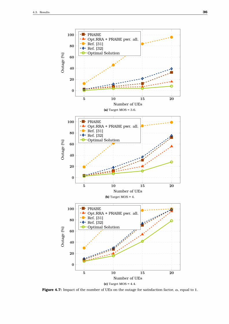
4.3. Results 36
5 10 15 20
0
20
40
60
80
100
Number of UEs
Ou
tage
(%)
PRABEOpt.RRA + PRABE pwr. all.Ref. [31]Ref. [32]Optimal Solution
(a) Target MOS = 3.6.
5 10 15 20
0
20
40
60
80
100
Number of UEs
Ou
tage
(%)
PRABEOpt.RRA + PRABE pwr. all.Ref. [31]Ref. [32]Optimal Solution
(b) Target MOS = 4.
5 10 15 20
0
20
40
60
80
100
Number of UEs
Ou
tage
(%)
PRABEOpt.RRA + PRABE pwr. all.Ref. [31]Ref. [32]Optimal Solution
(c) Target MOS = 4.4.
Figure 4.7: Impact of the number of UEs on the outage for satisfaction factor, α, equal to 1.
4.3. Results 37
80 85 90 95 100
0
20
40
60
80
100
Satisfaction Percentage (%)
Ou
tage
(%)
PRABEOpt.RRA + PRABE pwr. all.Optimal Solution
(a) Target MOS = 3.6.
80 85 90 95 100
0
20
40
60
80
100
Satisfaction Percentage (%)
Ou
tage
(%)
PRABEOpt.RRA + PRABE pwr. all.Optimal Solution
(b) Target MOS = 4.
80 85 90 95 100
0
20
40
60
80
100
Satisfaction Percentage (%)
Ou
tage
(%)
PRABEOpt.RRA + PRABE pwr. all.Optimal Solution
(c) Target MOS = 4.4.
Figure 4.8: Impact of the satisfaction factor on the outage for number of UEs, U , equal to 20.
4.3. Results 38
4.3.4 Imperfect CSI
The previous analyses considered perfect CSI, which is a simplified assumption. In this
section, we analyze the impact of considering imperfect CSI. Aiming to see only the effects
of the imperfect CSI, we consider a system with 5 UEs, since this is the only case where all
the algorithms present approximately zero outage for perfect CSI, as shown in Figure 4.2 of
Section 4.3.1.
Figure 4.9 presents the impact of the degradation, ξ, presented in (2.1), on the outage for
satisfaction factor, α, equal to 1. For target MOS equal to 3.6, in Figure 4.9(a), we note that in
the considered degradation interval, from 0% to 10%, the gap between the studied algorithms
is small and lower than 5%.
Changing the target MOS to 4, in Figure 4.9(b), the gap between [31] and the optimal
solution increases to 12%, while the gap between PRABE and the optimal solution is of
4%. Comparing Figures 4.9(a) and 4.9(b), it appears that [31] is more sensitive to the CSI
imperfections than the other algorithms.
Rising the target MOS to 4.4, in Figure 4.9(c), we can see that the imperfect CSI negatively
impacts all the algorithms, since their performance is very deteriorated even in a system
with only 5 UEs. However, it is important to note that the relative performance between the
algorithms do not change significantly from the ones obtained in the previous sections.
In this scenario, we also analyzed the impact of the satisfaction factor, since it has brought
gains in the other scenarios. Figure 4.10 presents similar evaluations but considering α equal
to 0.8 instead of 1, which means satisfy 4 users out of 5.
In Figure 4.10(a) we consider target MOS equal to 3.6. Comparing it to its equivalent with
α = 1, Figure 4.9(a), we can see an improvement in the performance of PRABE. Its outage has
decreased to values close to zero, which means that PRABE was able to satisfy 4 of 5 users in
almost all the simulations.
Figures 4.10(b) and 4.10(c) consider target MOS equal to 4 and 4.4, respectively. As
in Figure 4.10(a), the outage has been reduced if compared to their respective graphs in
Figure 4.9.
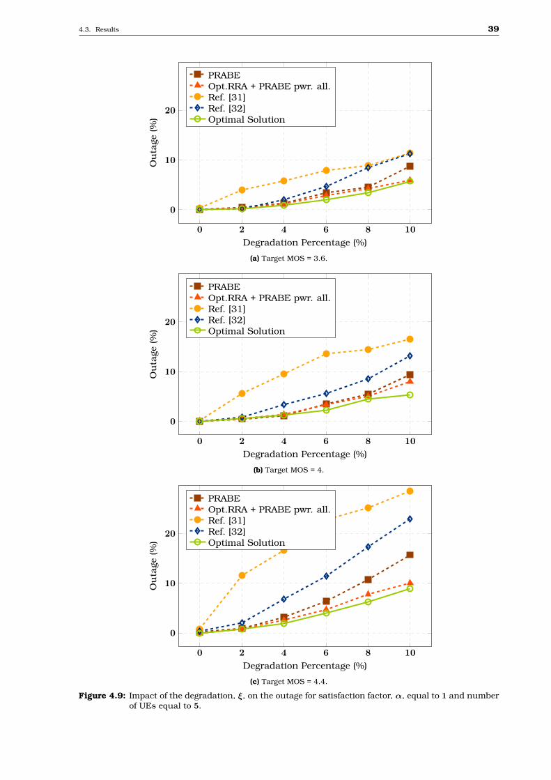
4.3. Results 39
0 2 4 6 8 10
0
10
20
Degradation Percentage (%)
Ou
tage
(%)
PRABEOpt.RRA + PRABE pwr. all.Ref. [31]Ref. [32]Optimal Solution
(a) Target MOS = 3.6.
0 2 4 6 8 10
0
10
20
Degradation Percentage (%)
Ou
tage
(%)
PRABEOpt.RRA + PRABE pwr. all.Ref. [31]Ref. [32]Optimal Solution
(b) Target MOS = 4.
0 2 4 6 8 10
0
10
20
Degradation Percentage (%)
Ou
tage
(%)
PRABEOpt.RRA + PRABE pwr. all.Ref. [31]Ref. [32]Optimal Solution
(c) Target MOS = 4.4.
Figure 4.9: Impact of the degradation, ξ, on the outage for satisfaction factor, α, equal to 1 and numberof UEs equal to 5.
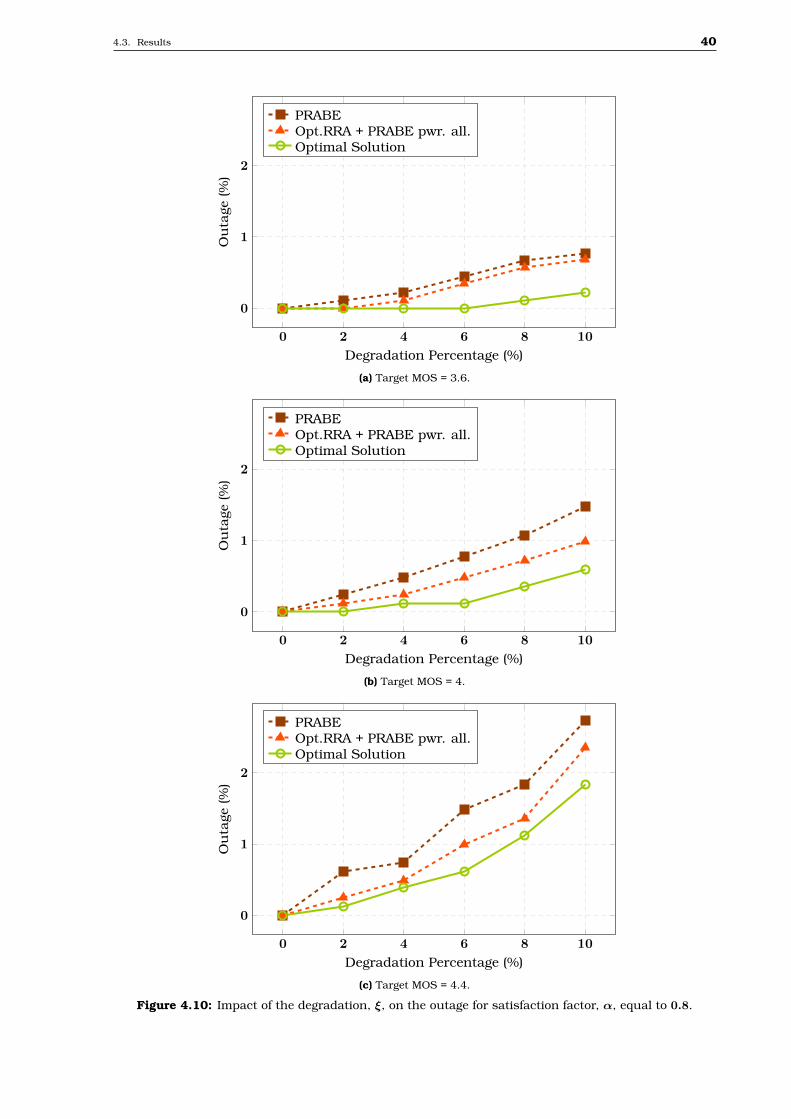
4.3. Results 40
0 2 4 6 8 10
0
1
2
Degradation Percentage (%)
Ou
tage
(%)
PRABEOpt.RRA + PRABE pwr. all.Optimal Solution
(a) Target MOS = 3.6.
0 2 4 6 8 10
0
1
2
Degradation Percentage (%)
Ou
tage
(%)
PRABEOpt.RRA + PRABE pwr. all.Optimal Solution
(b) Target MOS = 4.
0 2 4 6 8 10
0
1
2
Degradation Percentage (%)
Ou
tage
(%)
PRABEOpt.RRA + PRABE pwr. all.Optimal Solution
(c) Target MOS = 4.4.
Figure 4.10: Impact of the degradation, ξ, on the outage for satisfaction factor, α, equal to 0.8.
Chapter 5Conclusions and Future Work
In this master’s thesis, we have studied a new optimization problem in the fields of Quality
of Experience (QoE) and Radio Resource Allocation (RRA), taking into account constraints on
the total transmit power and on the fraction of users that must be satisfied.
More specifically, in Chapter 1, we have introduced some of the motivations that
are guiding operators to change their focus to delivering high-quality service experience,
independently of technical requirements. We have also presented an overview of what is
being doing in the three fields of QoE: modeling, measuring and optimization. Concerning
the optimization category, we have listed the main works that have already considered QoE
aspects when doing RRA.
In Chapter 3, a QoE-based RRA technique was studied from an optimization point of view.
We have mathematically formulated the problem of maximizing the minimum Mean Opinion
Score (MOS) of the users in a system constrained in transmit power and subject to satisfy
a minimum number of users called satisfaction factor. We were able to reformulate it as
a Mixed Integer Linear Problem (MILP), which solution can be obtained by standard solvers.
Motivated by the high computational effort required by the optimal solution, we have proposed
a framework called Power and Resource Allocation Based on Quality of Experience (PRABE).
In Chapter 4, we presented the performance evaluation. PRABE was evaluated in 4
different scenarios. The first one considered only one service plan. In this scenario, differently
from the benchmarking algorithms, PRABE performed very close to the optimal solution,
differing from it only for high values of target MOS and User Equipments (UEs) in the system.
In this case, the satisfaction factor reduction has enhanced PRABE’s performance. However,
as all UEs are treated as equal, any one can be chosen to not be satisfied.
To overcome this issue, in the second scenario, we divided the UEs into two service plans:
one with higher target MOS than the other. The obtained results validated the multi service
plans scenario as a good option to improve the system performance. We also evaluated the
reduction of the satisfaction factor of one of the plans, however the gains were marginals, if
we consider that we need to keep some users unsatisfied.
While the first two scenarios had a good coverage, the third one evaluated the performance
of PRABE in a scenario with worse coverage. The gap between PRABE and one of
the benchmarking algorithms has reduced in this analysis. However, it is important to
remark that PRABE still has a better performance and a less complex solution, since this
benchmarking algorithm uses the optimal solution of an optimization problem to allocate
power.
42
The last analyzed scenario studied the impact of considering imperfect Channel State
Information (CSI). As expected, the imperfect CSI negatively impacted all the algorithms.
However, the relative results between the algorithms did not change significantly from the ones
obtained in the other scenarios, where PRABE outperformed the benchmarking algorithms.
Some perspectives for the continuation of this master’s thesis work are listed below:
I Time extension: in this work, we considered that the users need to be satisfied at each
Transmission Time Interval (TTI). If we consider a satisfaction factor equal to one, this
assumption limits the number of UEs in the system to be at maximum the number of
Resource Blocks (RBs), since for higher quantities of UEs we are sure that someone will
not be allocated RBs leading to an unsatisfied state. Another approach could consider
that the users need to be satisfied in the average over a number of TTIs, this way we can
increase the number of UEs in the system. In this case, the target throughput rate of
each UE in each TTI will change according to the previous resource allocations.
I Multiple mapping functions: in this work, all the service plans have the same function
mapping throughput rate into MOS. However, it would be interesting to consider that
each service plan has its own mapping function.
I Mapping functions with other Quality of Service (QoS) parameters: another possible
extension to this work is to consider functions mapping other QoS parameters into MOS,
e.g. the delay, rather than just the throughput.
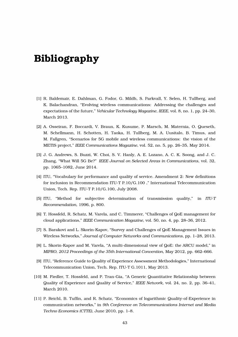
Bibliography
[1] R. Baldemair, E. Dahlman, G. Fodor, G. Mildh, S. Parkvall, Y. Selen, H. Tullberg, and
K. Balachandran, “Evolving wireless communications: Addressing the challenges and
expectations of the future,” Vehicular Technology Magazine, IEEE, vol. 8, no. 1, pp. 24–30,
March 2013.
[2] A. Osseiran, F. Boccardi, V. Braun, K. Kusume, P. Marsch, M. Maternia, O. Queseth,
M. Schellmann, H. Schotten, H. Taoka, H. Tullberg, M. A. Uusitalo, B. Timus, and
M. Fallgren, “Scenarios for 5G mobile and wireless communications: the vision of the
METIS project,” IEEE Communications Magazine, vol. 52, no. 5, pp. 26–35, May 2014.
[3] J. G. Andrews, S. Buzzi, W. Choi, S. V. Hanly, A. E. Lozano, A. C. K. Soong, and J. C.
Zhang, “What Will 5G Be?” IEEE Journal on Selected Areas in Communications, vol. 32,
pp. 1065–1082, June 2014.
[4] ITU, “Vocabulary for performance and quality of service. Amendment 2: New definitions
for inclusion in Recommendation ITU-T P.10/G.100 ,” International Telecommunication
Union, Tech. Rep. ITU-T P.10/G.100, July 2008.
[5] ITU, “Method for subjective determination of transmission quality,” in ITU-T
Recommendation, 1996, p. 800.
[6] T. Hossfeld, R. Schatz, M. Varela, and C. Timmerer, “Challenges of QoE management for
cloud applications,” IEEE Communication Magazine, vol. 50, no. 4, pp. 28–36, 2012.
[7] S. Barakovi and L. Skorin-Kapov, “Survey and Challenges of QoE Management Issues in
Wireless Networks,” Journal of Computer Networks and Communications, pp. 1–28, 2013.
[8] L. Skorin-Kapov and M. Varela, “A multi-dimensional view of QoE: the ARCU model,” in
MIPRO, 2012 Proceedings of the 35th International Convention, May 2012, pp. 662–666.
[9] ITU, “Reference Guide to Quality of Experience Assessment Methodologies,” International
Telecommunication Union, Tech. Rep. ITU-T G.1011, May 2013.
[10] M. Fiedler, T. Hossfeld, and P. Tran-Gia, “A Generic Quantitative Relationship between
Quality of Experience and Quality of Service,” IEEE Network, vol. 24, no. 2, pp. 36–41,
March 2010.
[11] P. Reichl, B. Tuffin, and R. Schatz, “Economics of logarithmic Quality-of-Experience in
communication networks,” in 9th Conference on Telecommunications Internet and Media
Techno Economics (CTTE), June 2010, pp. 1–8.
43
Bibliography 44
[12] A. Raake, J. Gustafsson, S. Argyropoulos, M. Garcia, D. Lindegren, G. Heikkila,
M. Pettersson, P. List, and B. Feiten, “IP-Based Mobile and Fixed Network Audiovisual
Media Services,” IEEE Signal Processing Magazine, vol. 28, no. 6, pp. 68–79, Nov 2011.
[13] M. Csernai and A. Gulyas, “Wireless Adapter Sleep Scheduling Based on Video QoE: How
to Improve Battery Life When Watching Streaming Video?” in Computer Communications
and Networks (ICCCN), 2011 Proceedings of 20th International Conference on, July 2011,
pp. 1–6.
[14] N. Amram, B. Fu, G. Kunzmann, T. Melia, D. Munaretto, S. Randriamasy, B. Sayadi,
J. Widmer, and M. Zorzi, “QoE-based transport optimization for video delivery over
next generation cellular networks,” in Computers and Communications (ISCC), 2011 IEEE
Symposium on, June 2011, pp. 19–24.
[15] K. Piamrat, A. Ksentini, C. Viho, and J. Bonnin, “QoE-based network selection for
multimedia users in IEEE 802.11 wireless networks,” in Local Computer Networks, 2008.
LCN 2008. 33rd IEEE Conference on, October 2008, pp. 388–394.
[16] F. Bendaoud, M. Abdennebi, and F. Didi, “Survey on scheduling and radio resources
allocation in lte,” International Journal of Next-Generation Networks, vol. 6, no. 1, pp.
17–29, March 2014.
[17] J. Jang and K. B. Lee, “Transmit Power Adaptation for Multiuser OFDM Systems,” IEEE
Journal on Selected Areas in Communications, vol. 21, no. 2, pp. 171–178, Jan. 2003.
[18] E. Yaacoub and Z. Dawy, Resource Allocation in Uplink OFDMA Wireless Systems: Optimal
Solutions and Practical Implementations. Wiley, 2012.
[19] D. Kivanc, G. Li, and H. Liu, “Computationally efficient bandwidth allocation and power
control for ofdma,” Wireless Communications, IEEE Transactions on, vol. 2, no. 6, pp.
1150–1158, November 2003.
[20] C. Y. Wong, R. S. Cheng, K. B. Lataief, and R. D. Murch, “Multiuser OFDM with
Adaptive Subcarrier, Bit, and Power Allocation,” IEEE Journal on Selected Areas in
Communications, vol. 17, no. 10, pp. 1747–1758, Oct. 1999.
[21] W. Rhee and J. M. Cioffi, “Increase in Capacity of Multiuser OFDM System Using
Dynamic Subchannel Allocation,” in Proceedings of the IEEE Vehicular Technology
Conference (VTC), vol. 2, May 2000, pp. 1085–1089.
[22] P. Patil and C. Borse, “Fair resource allocation to mimo wireless system using
opportunistic round robin scheduling algorithm,” in Pervasive Computing (ICPC), 2015
International Conference on, January 2015, pp. 1–3.
[23] E. Yaacoub and Z. Dawy, “Fair Optimization of Video Streaming Quality of Experience
in LTE Networks Using Distributed Antenna Systems and Radio Resource Management,”
Journal of Applied Mathematics, vol. 2014, no. Article ID 562079, pp. 1–12, July 2014.
[24] F. Chen, X. Qin, and G. Wei, “QoE Optimized Resource Allocation in Multiuser OFDM
Systems,” Przeglad Elektrochniczny (Electrical Review), vol. 2012, no. 7b, pp. 328–331,
July 2012.
Bibliography 45
[25] X. Chen, J.-N. Hwang, C.-N. Lee, and S.-I. Chen, “A near optimal qoe-driven power
allocation scheme for scalable video transmissions over mimo systems,” Selected Topics
in Signal Processing, IEEE Journal of, vol. 9, no. 1, pp. 76–88, Feb 2015.
[26] J. Zheng, Y. Cai, Y. Liu, Y. Xu, B. Duan, and X. Shen, “Optimal power allocation and
user scheduling in multicell networks: Base station cooperation using a game-theoretic
approach,” Wireless Communications, IEEE Transactions on, vol. 13, no. 12, pp.
6928–6942, Dec 2014.
[27] P. Tang, P. Wang, N. Wang, and V. N. Ngoc, “QoE-Based Resource Allocation Algorithm
for Multi-Applications in Downlink LTE Systems,” 2014 International Conference on
Computer, Communications and Information Technology (CCIT 2014), pp. 88–93, January
2014.
[28] X. Deng, Q. Gao, S. Mohammed, L. Chen, F. Wang, and Z. Fei, “A qoe-driven resource
allocation strategy for ofdm multiuser-multiservice system,” in Computer and Information
Technology (CIT), 2014 IEEE International Conference on, Sept 2014, pp. 351–355.
[29] Y. H. Cho, H. Kim, S.-H. Lee, and H. S. Lee, “A qoe-aware proportional fair resource
allocation for multi-cell ofdma networks,” Communications Letters, IEEE, vol. 19, no. 1,
pp. 82–85, Jan 2015.
[30] G. Lee, H. Kim, Y. Cho, and S.-H. Lee, “Qoe-aware scheduling for sigmoid optimization
in wireless networks,” IEEE Communications Letters, vol. 18, no. 11, pp. 1995–1998, Nov
2014.
[31] C. Sacchi, F. Granelli, and C. Schlegel, “A QoE-Oriented Strategy for OFDMA Radio
Resource Allocation Based on Min-MOS Maximization,” IEEE Communications Letters,
vol. 15, no. 5, pp. 494–496, May 2011.
[32] Z. Fei, C. Xing, and N. Li, “QoE-driven resource allocation for mobile IP services in
wireless network,” Science China Information Sciences, pp. 1–10, May 2014.
[33] A. Furuskär, “Radio Resource Sharing and Bearer Service Allocation for Multi-Bearer
Service, Multi-Access Wireless Networks,” Ph.D. dissertation, Royal Institute of
Technology (KTH), Radio Communication Systems, Apr. 2003.
[34] F. R. M. Lima, T. F. Maciel, W. C. Freitas, and F. R. P. Cavalcanti, “Resource Assignment
for Rate Maximization with QoS Guarantees in Multiservice Wireless Systems,” IEEE
Transactions on Vehicular Technology, vol. 61, no. 3, pp. 1318 –1332, Mar. 2012.
[35] F. R. M. Lima, T. F. Maciel, W. da Cruz Freitas Jr, and F. R. P. Cavalcanti, “Improved
Spectral Efficiency with Acceptable Service Provision in Multi-User MIMO Scenarios,”
IEEE Transactions on Vehicular Technology, vol. 63, no. 6, pp. 2697–2711, Jul. 2014.
[Online]. Available: http://dx.doi.org/10.1109/TVT.2013.2293333
[36] F. Capozzi, G. Piro, L. Grieco, G. Boggia, and P. Camarda, “Downlink Packet Scheduling
in LTE Cellular Networks: Key Design Issues and a Survey,” IEEE Communications
Surveys and Tutorials, vol. 15, no. 2, pp. 678–700, 2013.
[37] S. Sesia, I. Toufik, and M. Baker, LTE, the UMTS long term evolution : from theory to
practice, 2nd ed. John Wiley & Sons, 2011.
Bibliography 46
[38] 3GPP, “Evolved Universal Terrestrial Radio Access (E-UTRA); Physical channels and
modulation,” 3rd Generation Partnership Project (3GPP), TS 36.211, Mar. 2015. [Online].
Available: http://www.3gpp.org/ftp/Specs/html-info/36211.htm
[39] R. Fantacci, D. Marabissi, D. Tarchi, and I. Habib, “Adaptive modulation and coding
techniques for ofdma systems,” Wireless Communications, IEEE Transactions on, vol. 8,
no. 9, pp. 4876–4883, September 2009.
[40] 3GPP, “Evolved Universal Terrestrial Radio Access (E-UTRA); Radio Frequency (RF)
system scenarios,” 3rd Generation Partnership Project (3GPP), TR 36.942, Nov. 2014,
v.12.0.0. [Online]. Available: http://www.3gpp.org/dynareport/36942.htm
[41] ——, “Evolved Universal Terrestrial Radio Access (E-UTRA); Physical layer procedures,”
3rd Generation Partnership Project (3GPP), TS 36.213, Oct. 2010. [Online]. Available:
http://www.3gpp.org/ftp/Specs/html-info/36213.htm
[42] T. Maciel and A. Klein, “On the performance, complexity, and fairness of suboptimal
resource allocation for multiuser mimo-ofdma systems,” Vehicular Technology, IEEE
Transactions on, vol. 59, no. 1, pp. 406–419, January 2010.
[43] Y. J. Zhang and K. B. Letaief, “Multiuser Adaptive Subcarrier-and-Bit Allocation with
Adaptive Cell Selection for OFDM Systems,” IEEE Transactions on Communications, vol. 3,
no. 5, pp. 1566–1575, Sep. 2004.
[44] G. Nemhauser and L. Wosley, Integer and Combinatorial Optimization. John Wiley &
Sons, 1999.
[45] T. M. Apostol, One-Variable Calculus with an Introduction to Linear Algebra, 2nd ed.
Wiley, 1991.
[46] A. Cichocki, R. Zdunek, A. H. Phan, and S. ichi Amari, Nonnegative Matrix and Tensor
Factorizations: Applications to Exploratory Multi-way Data Analysis and Blind Source
Separation, 1st ed. Wiley, 2009.
[47] M. Bohge, “Dynamic Resource Allocation in Packet-Oriented Multi-Cell OFDMA Systems,”
Ph.D. dissertation, Berlin Technology University, Dec. 2010.
[48] F. Gunnarsson, M. Johansson, A. Furuskar, M. Lundevall, A. Simonsson, C. Tidestav,
and M. Blomgren, “Downtilted Base Station Antennas - A Simulation Model Proposal
and Impact on HSPA and LTE Performance,” in IEEE Vehicular Technology Conference,
September 2008, pp. 1–5.
[49] 3GPP, “Evolved universal terrestrial radio access (E-UTRA); further advancements for
E-UTRA physical layer aspects,” 3rd Generation Partnership Project (3GPP), TR 36.814,
Mar. 2010. [Online]. Available: http://www.3gpp.org/ftp/Specs/html-info/36814.htm
[50] ——, “Physical layer aspects for evolved universal terrestrial radio access (UTRA),” Third
Generation Partnership Project, TR 25.814 V7.1.0, Sep. 2006.
[51] ——, “Spatial channel model for multiple input multiple output (MIMO) simulations,”
Third Generation Partnership Project, TR 25.996 V7.0.0, Jun. 2007.
Bibliography 47
[52] C. Mehlführer, M. Wrulich, J. C. Ikuno, D. Bosanska, and M. Rupp, “Simulating
the long term evolution physical layer,” in Procedings of the European Signal
Processing Conference, Glasgow, Scotland, Aug. 2009. [Online]. Available: http:
//publik.tuwien.ac.at/files/PubDat_175708.pdf
[53] J. Poncela, G. Gomez, A. Hierrezuelo, F. Lopez-Martinez, and M. Aamir, “Quality
Assessment in 3G/4G Wireless Networks,” Wireless Personal Communications, vol. 76,
no. 3, pp. 363–377, 2014.
[54] IBM, “IBM ILOG CPLEX Optimizer.” [Online]. Available: http://www-01.ibm.com/
software/integration/optimization/cplex-optimizer/
[55] H. W. Kuhn, “The hungarian method for the assignment problem,” Naval Research
Logistics Quarterly, vol. 2, pp. 83–97, 1955.