
RADIATIVE CORRECTIONS AS THE ORIGIN OF … · RADIATIVE CORRECTIONS AS THE ORIGIN OF SPONTANEOUS...
82
arXiv:hep-th/0507214v1 21 Jul 2005 RADIATIVE CORRECTIONS AS THE ORIGIN OF SPONTANEOUS SYMMETRY BREAKING A thesis presented by Erick James Weinberg to The Department of Physics in partial fulfillment of the requirements for the degree of Doctor of Philosophy in the subject of Physics Harvard University Cambridge, Massachusetts May 1973
-
Upload
nguyendang -
Category
Documents
-
view
218 -
download
0
Transcript of RADIATIVE CORRECTIONS AS THE ORIGIN OF … · RADIATIVE CORRECTIONS AS THE ORIGIN OF SPONTANEOUS...
arX
iv:h
ep-t
h/05
0721
4v1
21
Jul 2
005
RADIATIVE CORRECTIONS AS THE ORIGIN OF
SPONTANEOUS SYMMETRY BREAKING
A thesis presented
by
Erick James Weinberg
to
The Department of Physics
in partial fulfillment of the requirements
for the degree of
Doctor of Philosophy
in the subject of
Physics
Harvard University
Cambridge, Massachusetts
May 1973
Abstract
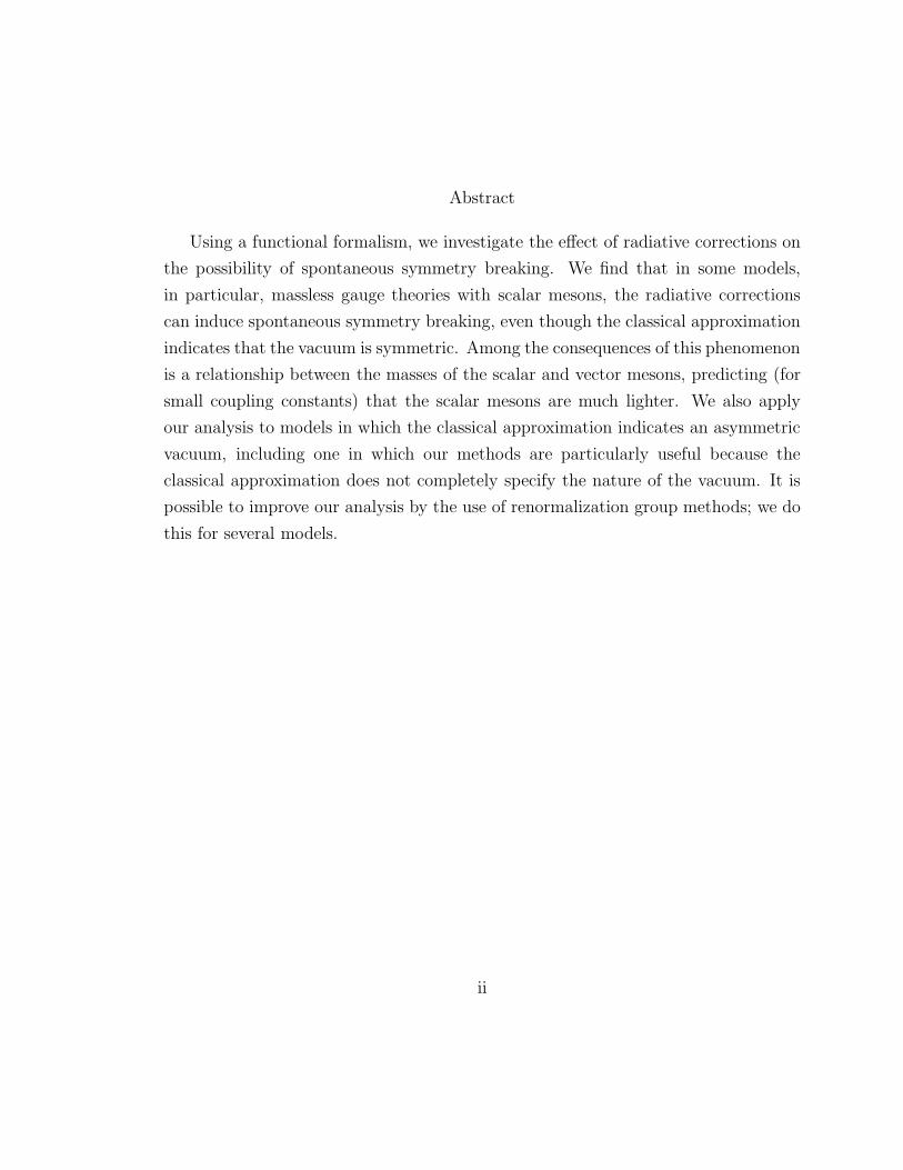
Using a functional formalism, we investigate the effect of radiative corrections on
the possibility of spontaneous symmetry breaking. We find that in some models,
in particular, massless gauge theories with scalar mesons, the radiative corrections
can induce spontaneous symmetry breaking, even though the classical approximation
indicates that the vacuum is symmetric. Among the consequences of this phenomenon
is a relationship between the masses of the scalar and vector mesons, predicting (for
small coupling constants) that the scalar mesons are much lighter. We also apply
our analysis to models in which the classical approximation indicates an asymmetric
vacuum, including one in which our methods are particularly useful because the
classical approximation does not completely specify the nature of the vacuum. It is
possible to improve our analysis by the use of renormalization group methods; we do
this for several models.
ii
Acknowledgments
I would like to thank my thesis advisor, Professor Sidney Coleman, for his assis-
tance and encouragement. I am grateful to him for showing me that the best way
to solve a difficult problem is often to not do the obvious. It has been a privilege to
have worked with him.
David Politzer has been of immeasurable assistance in this work; I have had
innumerable enjoyable and fruitful conversations with him. In addition, he has helped
me learn that two people working together can calculate Feynman diagrams with
neither can calculate alone.
I have profitted greatly from discussions with many faculty members, especially
Professors Thomas Appelquist, Sheldon Glashow, and Helen Quinn, as well as with
Dr. Howard Georgi.
I have learned a great deal from my fellow graduate students. I especially wish to
thank Jim Carazzone and Terry Goldman.
Teaching has been an enjoyable and rewarding experience; I thank Professors Paul
Bamberg and Arthur Jaffe for the opportunity to have taught with them.
I would like to thank Alan Candiotti for the use of his electric typewriter; without
it, this thesis would never have been finished.
Finally, I wish to thank my wife, Carolyn. Her love and understanding have
helped me through many of the dark and discouraging moments of graduate study.
iii
Table of Contents
Abstract ii
Acknowledgments iii
Chapter I. Introduction 1
Chapter II. Formalism 3
Chapter III. A Simple Example 10
Chapter IV. Bigger and Better Models 20
Chapter V. Massive Theories 33
Chapter VI. The Renormalization Group 46
Chapter VII. Conclusions 61
Appendix 62
Footnotes 63
Figures 65
iv
I. Introduction
Spontaneous symmetry breaking has been of great importance in the study of
elementary particles during the last decade, first because it explained why pions were
almost massless1, and then because it explained why weak intermediate vector mesons
did not have to be massless2. In all of its applications to particle physics, sponta-
neous symmetry breaking has been induced by writing the symmetric Lagrangian in
a somewhat unnatural manner — with a negative mass-squared term. In this paper
we will show that it is possible for a theory to have an asymmetric vacuum even
when the Lagrangian does not contain any such unnatural terms; instead, the spon-
taneous symmetry breaking is induced by the quantum corrections to the classical
field theory.3 In particular, theories which do not contain any mass terms may exhibit
this phenomenon; one may consider that the theory takes this form in order to avoid
the violent infrared divergences which would otherwise occur.
There are some interesting consequences when theories of this type display spon-
taneous symmetry breaking. The theory, originally formulated in terms of dimen-
sionless parameters, can be rewritten to show explicit dependence on a dimensional
quantity, namely the vacuum expectation value of one of the scalar fields. One of the
dimensionless parameters can be eliminated, and one obtains a relationship among
other quantities in the theory. In a gauge theory, this is generally a relationship
among masses, predicting a scalar meson mass which is much less that the vector
meson masses. We begin our discussion in Chapter II by describing a formalism
which is particularly suited to our purposes. In Chapter III we apply our methods
to the study of a particularly simple model, where we do not find evidence of spon-
taneous symmetry breaking. In Chapter IV we introduce more complicated theories,
including some where the vacuum is asymmetric. All of the models considered in
Chapters III and IV are without mass terms. In Chapter V we show how these can
be embedded in the more general class of theories with mass terms (of either sign).
We also give an example where our methods are particularly useful, even though the
classical treatment of the theory already predicts spontaneous symmetry breaking.
In Chapter VI we show how the methods of the renormalization group allow us to
1
improve the analysis of Chapters III and IV. We list our conclusions in Chapter VII.
An appendix discusses the relationship between our results and a theorem of Georgi
and Glashow.
2
II. Formalism
In the usual treatment of spontaneous symmetry breaking in quantum field theory,
one assumes that by looking at the Lagrangian of a particular theory it is possible to
determine whether or not the theory displays spontaneous symmetry breaking. That
is, one defines the negative of the non-derivative terms in the Lagrangian to be a
potential, assumes that all fields are constant in space-time in the vacuum state, and
minimizes the potential as a function of the fields to determine the expectation value
of the fields in the vacuum state. If the vacuum expectation value of some field is non-
invariant under some symmetry of the Lagrangian, spontaneous symmetry breaking
is said to occur.
In a classical field theory, this would be precisely the thing to do. In a quantum
field theory, this procedure is approximate at best, since the quantized fields are
non-commuting operators and one must be careful in manipulating them. To put
things differently, the operator nature of the fields gives rise to internal loops in
Feynman diagrams; that is, there are both radiative corrections to the interactions
in the Lagrangian and new interactions which are not explicit in the Lagrangian.
These effects are clearly relevant in determining the nature of the vacuum; the usual
assumption is that their effect is only to make small quantitative changes and that
the classical approximation gives a correct qualitative description of the vacuum.
Since we are interested in considering cases where this assumption may be false,
it is desirable to use a formalism which treats the classical approximation and the
quantum corrections on the same basis.
Such a formalism is provided by the functional methods introduced by Schwinger
and developed by Jona-Lasinio, whose treatment we follow4. These method enable
us to define an effective potential which includes all the interactions of the theory,
both those explicit in the Lagrangian and those arising from quantum corrections.
Furthermore, this effective potential is a function of classical fields, so it can be easily
manipulated. Finally, its minima determine the nature of the ground state of the
theory.
One begins by adding to the Lagrangian a coupling to external c-number sources,
3
one source for each field in the theory; that is,
L(φi, ∂µφi) → L(φi, ∂
µφi) +∑
i
φi(x)Ji(x) , (2.1)
where the φi represent all the fields of the theory, whatever their spin. Next one
defines a functional W (J) in terms of the probability amplitude for the vacuum state
in the far past to go into the vacuum state in the far future in the presence of the
external sources:
eiW (J) = 〈0+|0−〉 . (2.2)
The importance of W (J) lies in the fact that it is the generating functional for the
connected Green’s functions; that is, we can write
W (J) =∑
n1,n2,...,nk
1
n1!n2! . . . nk!
∫
d4x1d4x2 . . . d
4xn1. . . d4wnk
×G(n1,n2,...,nk)(x1, x2, . . . , wnk)J1(x1)J1(x2) . . . J1(xn1
) . . . Jk(wnk) .
(2.3)
Here G(n1,n2,...,nk)(x1, x2, . . . , wnk) is the sum of all connected Feynman diagrams with
n1 external lines of type 1, n2 external lines of type 2, etc.
Now one defines classical fields Φic(x) by
Φic(x) =δW (J)
δJi(x)=
〈0+|φi(x)|0−〉J〈0+|0−〉J
. (2.4)
Finally, we define the effective action, Γ(Φc), by a functional Legendre transformation:
Γ(Φc) = W (J) −∑
i
∫
d4xJi(x)Φic(x) . (2.5)
From Eq. (2.5) we can immediately conclude that
δΓ(Φc)
δΦic(x)= −Ji(x) . (2.6)
The effective action is also a generating functional; it can be written
Γ(Φc) =∑
n1,n2,...,nk
1
n1!n2! . . . nk!
∫
d4x1d4x2 . . . d
4xn1. . . d4wnk
× Γ(n1,n2,...,nk)(x1, x2, . . . , wnk)Φ1c(x1)Φ1c(x2) . . .Φ1c(xn1
) . . .Φkc(wnk) .
(2.7)
4
The Γ(n1,n2,...,nk)(x1, x2, . . . , wnk) are the IPI (one-particle-irreducible) Green’s func-
tions, defined as the sum of all connected Feynman diagrams which cannot be dis-
connected by cutting a single internal line; these are evaluated without propagators
on the external lines.
Although Eq. (2.7) is the usual expansion of the effective action, it is not the one
best suited for studying the possibility of spontaneous symmetry breaking. A better
expansion is obtained by expanding in powers of the external momenta about the
point where all external momenta are zero; in other words, a Taylor series expansion
about a constant value, ϕic, of the classical fields Φic(x). In this expansion we do
not distinguish terms with different numbers of external scalar particles, but we do
distinguish terms with different number of external particles with spin. Thus, for a
theory containing a scalar field, φ, and a vector field, Aµ, this expansion would look
like
Γ(Φc) =∫
d4x{
−V (ϕc) +1
2∂µΦc(x)∂
µΦc(x)Z(ϕc)
+∂µΦc(x)Aµc (x)Φc(x)G(ϕc) + Φc(x)
2Aµc2H(ϕc) + AµcA
µcK(ϕc) + · · ·
}
.
(2.8)
Note that the coefficients in this expansion are functions, not functionals. The first
term, V (ϕc), is called the effective potential; it is equal to the sum of all Feynman
diagrams with only external scalar lines and with vanishing external momenta. Those
diagrams without loops correspond to the interactions in the Lagrangian, while those
with loops correspond to the quantum corrections.
Now we wish to see how spontaneous symmetry breaking is described in this
formalism. We assume that the Lagrangian possesses a symmetry which is sponta-
neously broken if some field acquires a non-zero vacuum expectation value. From
Eq. (2.4) we see that if the external sources vanish, the classical field is just the vac-
uum expectation value of the quantized field; this observation, plus Eq. (2.6), tells us
that the condition for spontaneous symmetry breaking is
δΓ(Φc(x))
δΦc(x)= 0 , for Φc(x) 6= 0 . (2.9)
Since spontaneous breaking of Poincare invariance does not seem to be a physically
5
significant phenomenon, we will restrict ourselves to theories in which the vacuum
is invariant under translation. If the Lagrangian and the quantization procedure
are also Poincare invariant, then the vacuum expectation value of the fields will be
constant in space-time, and Eq. (2.9) reduces to
dV (ϕc)
dϕc= 0 , for ϕc 6= 0 . (2.10)
Thus we have obtained, as promised, a c-number function whose minimum deter-
mines the nature of the ground state. In fact, the effective potential can give us much
more information. If we compare Eqs. (2.7) and (2.8), we see that the nth derivative
of V (ϕc), evaluated at ϕc = 0, is just the n-point IPI Green’s functions, evaluated
at zero external momenta. Of particular interest is the 2-point IPI Green’s function,
which is the inverse propagator; its value at zero momentum may be taken as the def-
inition of the mass. (It is not exactly the position of the pole in the propagator, but
we usually expect it to be close.) Thus, in a theory without spontaneous symmetry
breaking, we may write the scalar meson mass matrix as
m2ij =
∂2V
∂ϕi∂ϕj
∣
∣
∣
∣
∣
ϕc=0
. (2.11)
If spontaneous symmetry breaking does occur, then Eq. (2.11) no longer holds, since
the mass is defined for an isolated particle; that is, the inverse propagator must be
evaluated in the ground state. To do this, we make the usual redefinition of the scalar
fields; if 〈ϕ〉 is the vacuum expectation value of φ, we define a new quantum field, φ′,
and a new classical field, Φ′c, by
φ′(x) = φ(x) − 〈ϕ〉 (2.12)
and
Φ′(x) = Φ(x) − 〈ϕ〉 . (2.13)
The mass matrix is then given by
m2ij =
∂2V
∂ϕ′ic∂ϕ
′jc
∣
∣
∣
∣
∣
ϕ′
c=0
=∂2V
∂ϕic∂ϕjc
∣
∣
∣
∣
∣
ϕc=〈ϕ〉
. (2.14)
6
There is an additional advantage of the functional formalism, which we will not
make use of, but which is worth pointing out: Instead of coupling the external sources
in Eq. (2.1) to the elementary fields of the theory, we could have coupled them to
more complicated fields. We would then have obtained a set of classical fields which
would not have simple relationships to the elementary quantum fields of the theory.
This might be desirable in at least two different cases. First, it allows one to study
the possibility of spontaneous symmetry breaking in a theory without elementary
scalar fields, by having a compound field, rather than an elementary field, acquire
a non-zero vacuum expectation value. Second, it has the possibility of describing
strong interaction effects in terms of the phenomenological fields, even though these
fields quite likely cannot be simply expressed in terms of the fundamental quantum
fields.
Thus the study of spontaneous symmetry breaking is reduced to the calculation of
the effective potential. Unfortunately, this is not so simply done; even if one accepts
the validity of a calculation to all orders of perturbation theory, such a calculation
requires summing an infinite number of Feynman diagrams, which is no mean feat.
It is therefore necessary to find an approximation for the effective potential which
will require the summation of only some subset of the relevant Feynman diagrams.
The first expansion to come to mind is that which is most often used in perturba-
tion theory: expansion in powers of the coupling constants. However, there are two
objections to using this method for the problem at hand. First, in theories with spon-
taneous symmetry breaking one commonly defines shifted fields, with a corresponding
redefinition of the coupling constants. This can lead to confusion in comparing the
order of diagrams calculated using different shifts. But this can be unraveled if one is
careful; it certainly does not invalidate the method. The second objection is more ba-
sic: We will often be considering theories which appear to contain massless particles,
for example, massless scalar electrodynamics. Two diagrams which contribute to the
effective potential in scalar electrodynamics are shown in Fig. 1. The first is of order
e4, while the second is of order e24. An expansion in powers of coupling constants
assumes that the second is negligible in comparison with the first, while in fact it is
7
much more infrared divergent, and not at all negligible. This is not merely a fluke
which occurs because we happen to have considered a theory with massless particles.
Spontaneous symmetry breaking, like critical phenomena in many-body theory, is as-
sociated with correlations between widely separated points; the presence of massless
particles, which can mediated long-range forces, is obviously of extreme importance.
In fact, if one tried to study massless scalar electrodynamics and neglected diagrams
such as that in Fig. 1b, one would obtain qualitatively different results.
A better approximation is the expansion by the number of loops in a diagram5.
First, let us show that such an expansion is unaffected by a shift of the fields. We
introduce a parameter b into the Lagrangian by writing
L(φi, ∂µφi; b) = b−1L(φi, ∂
µφi) . (2.15)
The power, P , of b associated with a particular diagram will be
P = I − V , (2.16)
where I is the number of internal lines and V is the number of vertices, since the ver-
tices are obtained from the interaction Lagrangian while the propagators are obtained
from the inverse of the free Lagrangian. The number of loops, L, is equal to the num-
ber of independent internal momenta. This is equal to the number of momenta (I),
less the number of energy-momentum delta functions (V ), but not counting the delta
function corresponding to overall energy-momentum conservation. In other words
L = I − V + 1 = P + 1 . (2.17)
We see that the number of loops is determined by the power of a quantity which
multiplies the whole Lagrangian, and does not depend on the details of how the
Lagrangian was written; thus the loop expansion is unaffected by a redefinition of
the fields.
It still remains to be seen whether the loop expansion is a good approximation.
Certainly the appearance of high powers of b does not make a diagram small, since b
must be set equal to one. However, many-loop diagrams must contain many powers
8
of the coupling constants, so the loop expansion is at least as good as the coupling
constant expansion. Also, diagrams such as that in Fig. 1b are included in the same
order as that in Fig.1a, so the second objection to the coupling constant expansion
is avoided. (One may ask why certain two-loop graphs, such as that in Fig. 2, are
any less important than that in Fig. 1b; the answer will appear presently.) We shall
see as we go on that logarithms will appear in our calculations, and that the validity
of the loop expansion will require not only that the coupling constants, but also the
logarithms, be small. (Similarly, logarithms appear in the usual applications of the
coupling constant expansion, where one expects the results to hold only when the
logarithms are small.)
Finally, we note that the zero-loop (tree) approximation is equivalent to treating
the theory classically.
At this point it is probably most instructive to consider a specific model in order
to see how our methods work.
9
III. A Simple Example
Let us consider a simple, but illustrative, model: the theory of a single quartically
self-coupled scalar field. The Lagrangian for the theory is 6
L =1
2(∂µφ)2 − 1
2m2φ2 − λ
4!φ4 +
A
2(∂µφ)2 − B
2φ2 − C
4!φ4 , (3.1)
where the last three terms are counter-terms to be determined, order by order in the
loop parameter, by the renormalization conditions. The coupling constant, λ, may be
either positive or negative. Ordinarily one forbids negative λ on the grounds that it
leads to a potential which has no lower bound, but of course this is a statement only
about the zero-loop approximation to the effective potential; the loop contributions
may (or may not) be such as to put a lower bound on the effective potential, even
for negative λ.
The theory contains a discrete symmetry, namely φ → −φ. The conventional
wisdom (for positive λ) is that the vacuum is symmetric if m2 is positive, and that
spontaneous symmetry breaking occurs if m2 is negative. (Goldstone’s theorem does
not apply, since there is no continuous symmetry.) However, the conventional wisdom
does not say very much about the case where m2 vanishes, except to warn of the
terrible infrared divergences which may arise. In fact, this case is not well defined until
the renormalization conditions are specified. Let us choose the mass renormalization
so thatd2V
dφ2c
∣
∣
∣
∣
∣
ϕc=0
= m2 = 0 . (3.2)
If the vacuum occurs when ϕc = 0, this means that the inverse propagator at zero
external momentum vanishes; in other words, the theory really contains a massless
particle. On the other hand, if spontaneous symmetry breaking occurs, this is not a
condition on the physical inverse propagator and there is not necessarily a massless
particle; one might ask why this should be considered a special case. The reason is
that the point ϕc = 0 is a symmetric one, and the symmetric formulation of a theory
is significant; for example, the unitary gauge of a Higgs theory may be useful for
calculating amplitudes, but the renormalizable gauge is certainly better for under-
standing the underlying symmetries of the theory. In any case, let us consider the
10
theory with m2 = 0, and see whether spontaneous symmetry breaking occurs. (We
still have not completely specified the theory, since the wave function and coupling
constant renormalization conditions have not been stated, but these are best left for
later, when their motivation will be more apparent.
One last task remains before we can begin calculating the effective potential:
we must learn how to count i’s, minus signs, and factorials. A term gφn in the
Lagrangian leads to a Feynman diagram with n external φ lines and a value of ig(n!).
Remembering that the Lagrangian contains the negative of the potential, we see that
the contribution to the effective potential from a diagram with n external lines is
i
n!ϕn
c × (diagram) . (3.3)
In the zero-loop approximation only one diagram, that shown in Fig. 3, contributes
to the effective potential. Its contribution is, of course,
Vzero−loop =λ
4!ϕ4
c , (3.4)
In the next order we have the infinite series of diagrams shown in Fig. 4a, as well as
the diagrams of Fig. 4b, which arise from the one-loop mass and coupling constant
counter-terms. The latter clearly do not contain any loops, but they are to be counted
here because we are really expanding in powers of the loop-counting parameter, b,
and these terms are of order b0.
In calculating the contribution from the diagrams of Fig. 4a, we must keep track
of certain combinatoric factors. To understand these, let the external lines have small
non-zero momenta, ǫ1, ǫ2, . . . , ǫ2n. (Ultimately, we will let these momenta go to zero.)
We now count the one-loop diagrams with 2n external lines. First, we consider the
case where n ≥ 3. We note the following:
1) There are (2n)! ways of arranging the external momenta.
2) Interchanging the external moment at a vertex does not give a new diagram,
so we have a factor of (12)n.
3) Rotating or reflecting a diagram does not give a new diagram, so we have
another factor of 1/(2n).
11
The contributions from one-loop diagrams with 2n external lines (n ≥ 3) is thus
[
(2n!)(
1
2
)n 1
2n
]
[
i
(2n)!ϕ2n
c
]
(diagram) =i
2n
(
ϕ2c
2
)n
(diagram) . (3.5)
If n equals 1 or 2, point (3) must be modified. For n = 1, the diagram cannot be
reflected or rotated; for n = 2, reflection and rotation are the same, so there is only
a factor of 1/2, rather than 1/4. However, in both of these cases the Feynman rules
include an extra factor of 1/2.
We can now write an expression for the one-loop approximation to the effective
potential:
Vone−loop approx =λ
4!ϕ4
c +∞∑
n=1
∫ d4k
(2π)4
[
i
2n
(
λϕ2c/2
k2 + iǫ
)n]
+B(1)
2ϕ2
c +C(1)
4!ϕ4
c . (3.6)
We notice that the integrals for n ≥ 2 are infrared divergent. We also notice that the
infinite sum can be done, yielding
Vone−loop approx =λ
4!ϕ4
c +i
2
∫ d4k
(2π)4log
(
1 − λϕ2c/2
k2 + iǫ
)
+B(1)
2ϕ2
c +C(1)
4!ϕ4
c . (3.7)
The infrared divergence has disappeared, being replaced by a logarithmic singularity
at the origin of classical field space. It is not too surprising that this should occur,
since we expect infrared divergences only if the vacuum is at ϕc = 0. If spontaneous
symmetry breaking occurs, then φ does not remain massless, and there is no reason
to expect infrared problems.
We do the integral by rotating into Euclidean space and cutting off the integral
at k2 = Λ2. We obtain
Vone−loop approx =λ
4!ϕ4
c +1
64π2
{
λϕ2cΛ
2 +λϕ4
c
4
[
logλϕ2
c
2Λ2− 1
2
]}
+B(1)
2ϕ2
c +C(1)
4!ϕ4
c .
(3.8)
We must now determine the value of the renormalization counter-terms. The mass
renormalization condition was given in Eq. (3.2). From it we deduce that
B(1) = − λΛ2
32π2. (3.9)
12
Now we come to the coupling constant renormalization condition, which we have left
unspecified so far. Two possibilities are
d4V
dϕ4c
∣
∣
∣
∣
∣
ϕc=0
= λ (3.10a)
and4!
ϕ4c
V
∣
∣
∣
∣
∣
ϕc=0
= λ . (3.10b)
Unfortunately, neither of these is acceptable, because of the logarithmic singularity
at the origin of the classical field space. Instead, we choose an arbitrary value of ϕc,
which we denote by M , and require either
d4V
dϕ4c
∣
∣
∣
∣
∣
ϕc=M
= λ (3.11a)
or4!
ϕ4c
V
∣
∣
∣
∣
∣
ϕc=M
= λ . (3.11b)
It is important to remember that the choice of M is arbitrary; if a different value is
chosen for M , one obtains a different value for λ, but the theory remains unchanged.
In other words, as M is varied λ traces out a curve λ(M). Although two parameters
appear, there is actually only a one-parameter family of theories, one theory for
each curve. We shall return to this point later, when we discuss the use of the
renormalization group. (Note that this is analogous to what happens in the usual
treatment of theories with massless particles. Because of the infrared divergences,
some of the renormalizations cannot be done at zero external momentum; instead,
they are done at an arbitrary non-zero momentum.)
For the moment, let us choose Eq. (3.11a) as the renormalization condition, since
it is closer to the definition of the physical 4-point IPI Green’s function. (It is, in
fact, the definition of the physical Green’s function if M is equal to the vacuum
expectation value of φ.) We find
C(1) = − 3λ2
32π2
(
logλM2
2Λ2+
11
3
)
(3.12)
13
and
Vone−loop approx =λ
4!ϕ4
c +λ2ϕ4
c
256π2
[
logϕ2
c
M2− 25
6
]
. (3.13)
We note several things about our final expression for the effective potential:
1) V still contains the logarithmic singularity in φc, but the singularity at λ = 0
has disappeared.
2) M is in fact arbitrary; if we let M go to M ′, we can choose a new coupling
constant,
λ′ =d4V
dϕ4c
∣
∣
∣
∣
∣
ϕc=M ′
= λ+3λ2
32π2log
M ′2
M2, (3.14)
and find
V =λ′
4!ϕ4
c +λ′2ϕ4
c
256π2
[
logϕ2
c
M ′2− 25
6
]
. (3.15)
This, to the order of approximation to which we are working, describes the same
theory as Eq. (3.13)
3) The behavior of V is shown in Fig. 5. Since the logarithm of a small number
is negative, it appears that there is a maximum at the origin and a minimum at a
non-zero value of ϕc. Differentiating V , we find
dV
dϕc
=λ
6ϕ3
c +λ2ϕ3
c
64π2
[
logϕ2
c
M2− 11
3
]
. (3.16)
Thus the minimum occurs at a value of ϕc determined by
λ logϕ2
c
M2− 11λ
3= −32π2
3. (3.17)
Thus it would appear that this theory exhibits spontaneous symmetry breaking. How-
ever, we must consider the effects of many-loop diagrams, and see whether there are
solutions of Eq. (3.17) which are consistent with the validity of the one-loop approx-
imation.
It turns out that increasing the number of loops brings in not only additional
powers of λ, but also additional logarithms; that is, the leading behavior of the n-
loop contribution to the effective potential is of the order of
λ
(
λ logϕ2
c
M2
)n
. (3.18)
14
Thus the one-loop approximation can be valid only if both |λ| and |λ log(ϕ2c/M
2)| are
small. However, it is clear that Eq. (3.17) cannot be satisfied unless one of these is
large. There may be a minimum of the effective potential away from the origin, but
if there is, it is in a region where our calculational methods fail. Similarly, we cannot
trust the prediction that there is a maximum at the origin. Later we shall see that
by the use of the methods of the renormalization group we can improve the situation,
but for the present we simply do not know whether spontaneous symmetry breaking
occurs.
Of course, we should not be too surprised that our approximation did not give us
any reliable evidence of spontaneous symmetry breaking. The zero-loop approxima-
tion to the effective potential indicates that spontaneous symmetry breaking does not
occur. If we want the one-loop approximation to change this, we should expect that it
must be of the same order of magnitude as the zero-loop term; this is possible only if
the interaction is strong, in which case a perturbative methods is expected to fail. At
this point, we might conclude that our methods will never indicate spontaneous sym-
metry breaking unless it is already predicted by the classical approximation; however,
this is not quite true.
Consider a theory with two interactions, A and B. Suppose that only A con-
tributes to the effective potential in the zero-loop approximation, but that B con-
tributes through loop diagrams. Even if A and B are both weak, it may be possible
to make the one-loop B contribution and the zero-loop A contribution be of the same
order of magnitude by adjusting the relative strength of A and B. If so, the one-loop
contributions might give rise to spontaneous symmetry breaking, not because they
are large, but because they involve a new type of interaction. Since both interactions
are weak, and there are no other interactions to be introduced, the contributions from
diagrams with two or more loops should be small; therefore, the one-loop approxi-
mation should be valid.
One might ask whether it is possible to construct a theory in which the loop
expansion is valid, but in which the diagrams with two or more loops introduce new
interactions which qualitatively change the effective potential; we not found any. To
15
see the difficulty, consider the electrodynamics of a scalar with charge e and a fermion
with charge g, with an additional quartic scalar self-coupling with coupling constant
λ. The zero-loop approximation to the effective potential will be of the order of λ,
while the one-loop contributions will be of the order of λ2 or e4. The fermion-photon
interaction first contributes in the two-loop approximation, through corrections to
the photon propagator. These contributions will be of the order of g2e4; for these to
be significant in comparison with the one-loop terms, g2 must be large, in which case
the perturbation theory is no longer valid.
Let us now justify Eq. (3.18) by deriving some simple rules which make it possible
to sum all the graphs of any particular order as easily as we summed all of the one-loop
graphs. Consider, for example, the two-loop graphs of the type shown in Fig. 6a. To
obtain the contribution of these graphs to the effective potential, we must sum over
all values of l, m, and n from zero to infinity. In doing the sum, we must remember
the following factors:
1) A factor of (2l + 2m+ 2n)!, which cancels the factorial in Eq. (3.3), just as in
the one-loop calculation.
2) A factor of (1/2)l+m+n, from interchanging the lines at each of the vertices with
two external lines; this also is analogous to the one-loop calculation.
3) A factor of 1/(3!), arising from the symmetry of the diagram.
We can do the sums over l, m, and n independently. Each sum is of the form
∞∑
j=0
(
−iλϕ2c
2
)j (i
k2 + iǫ
)j+1
=i
k2 − 12λϕ2
c + iǫ. (3.19)
In addition we have a factor of −iλϕc at each of the two remaining vertices and the
factor of 1/6 from point (3). This is just what we would have obtained from the
graph of fig. 6b if the φ had a mass of 12λϕ2
c . (The Feynman rules would include the
1/6, again from the symmetry of the graph.) We shall call those graphs which, like
that in Fig. 6b, have no vertices with two external lines prototype graphs. It is clear
that the above discussion holds for all prototype graphs. We thus obtain a rule for
calculating the n-loop contribution to the effective potential: Draw all of the n-loop
prototype graphs and calculate them using ordinary Feynman rules, except with a
16
propagator given by Eq. (3.19). The only exception to this rule is the case of one-loop
graphs, which alone are invariant under rotation. We note that the prototype graph
in this case is a circle, which does not correspond to any Feynman diagram arising
from ordinary perturbation theory.
All that remains is to show that there are a finite number of n-loop prototype
graphs. We define a type-n vertex to be one with n internal lines, and denote the
number of type-n vertices in a graph by Vn. By definition, an IPI graph does not
contain any type-1 vertices, while a prototype graph contains only type-3 and type-4
vertices. For an IPI graph,
V = V2 + V3 + V4 . (3.20)
Since every internal line has two ends, we see that
2I = 2V2 + 3V3 + 4V4 . (3.21)
Thus,
L = I − V + 1 =1
2V3 + V4 + 1 . (3.22)
Thus, for a given L, only a finite number of type-3 and type-4 vertices are allowed.
Since only a finite number of graphs can be made with a given finite number of
vertices, the number of prototype graphs in any order is finite.
A few words of caution:
1) One must not forget diagrams arising from the insertion of counter-terms.
These are calculated by drawing prototype graphs with counterterm insertions drawn
explicitly, remembering that the order of the counter-term must be included in de-
termining the order of a diagram. The number of such prototype graphs in any order
is finite, since all counter-terms are at least one-loop in order.
2) The factor of 12λϕ2
c in Eq. (3.19) looks like a mass, but it is not; it is not
even a constant. However, it is related to the mass if ϕc is set equal to the vacuum
expectation value of φ.
3) One must remember that we are summing all IPI graphs, and that the use
of prototype graphs is merely a device to perform the sum. Thus we must include
the prototype graph in Fig. 7, even though it has no external lines. The reason is
17
that this prototype graph stands for a sum of graphs which do have external lines.
However, it also includes the graph which looks exactly like it and which does not
have any external lines; this graph must be subtracted after the prototype graph is
calculated. That is, the total contribution of this prototype graph to the effective
potential is
i(−iλ)
[
1
2
∫
d4k
(2π)4
i
k2 − 12λϕ2
c + iǫ
]2
−[
1
2
∫
d4k
(2π)4
i
k2 + iǫ
]2
. (3.23)
We can now calculate some many-loop graphs, and verify Eq. (3.18). It is now
also possible to specify the wave function renormalization condition, which we have
not yet done. This is a condition on the term in the effective action which is of the
form
∂µΦc∂µΦcZ(ϕc) . (3.24)
In the zero-loop approximation, Z will be 1. The one-loop contribution to Z
arises from the counter-term and from the one-loop diagrams which have two external
φ’s with four-momenta p and −p, and any number of external φ’s with vanishing
four-momenta. (Actually, it is just the term proportional to p2 in the Taylor series
expansion of these diagrams.) The sum of these diagrams can be calculated using
the methods outlined above: one draws prototype graphs in which the vertices with
non-vanishing external momenta are shown explicitly, while the vertices with two
zero-momentum external lines are implicit in the propagators. The resulting integrals
have ultra-violet divergences and must be cut off; a counter-term is necessary to make
Z cutoff-independent. The most natural choice for the renormalization condition is
Z(0) = 1 . (3.25)
Unfortunately, the same difficulty arises here as arose with the coupling constant
renormalization: Z contains a logarithmic singularity at ϕc = 0. Thus, we must
renormalize at some arbitrary non-zero value of ϕc. For simplicity, we choose the
value we used for the coupling constant renormalization, and have
Z(M) = 1 . (3.26)
18
Again we see the similarity to the usual method of renormalization in momentum-
space. There, the wave function renormalization, like the coupling constant renor-
malization, would have an infrared divergence, while the mass renormalization would
not; in our method, the first two have logarithmic singularities, while the third does
not.
19
IV. Bigger and Better Models
In this chapter we shall extend the methods of the previous chapter to models
which include more than one field; we shall continue, however, to restrict ourselves to
models in which no mass term appears in the Lagrangian. (As mentioned previously,
this does not necessarily imply that the theory contains massless particles.) We shall
also restrict ourselves to renormalizable theories, since only for these do we have any
assurance that higher order calculations will be finite.
In a theory with many quantized fields, we find it useful to define a classical
field corresponding to each quantized field; the effective action is a functional of all
these classical fields. However, in expanding Γ in Eq. (2.8), we defined the effective
potential to depend only on the spinless classical fields. The reason is that we are
only interested in cases where the vacuum is Lorentz invariant; therefore we want the
vacuum expectation value of any field with spin to be zero.
Just as with the theory of a single scalar field, it is possible to derive rules which
enable us to sum the infinite number of Feynman diagrams which occur in each order
in the loop expansion. We begin by considering graphs that contain only spin-zero
particles. We arrange the real spinless fields in a vector ~φ, with components φi. (One
should not be misled by the notation to conclude that these fields necessarily belong
to a representation of some symmetry group.) Also, we define V0(~ϕc) to be the zero-
loop approximation to the effective potential. (It is, of course, of the same form as
the potential terms in the Lagrangian, except that it is a function of the classical,
rather than of the quantized, fields.) Finally, we define a matrix U(~ϕc) by
Uij(~ϕc) =∂V0(~ϕc)
∂ϕic∂ϕjc. (4.1)
This is exactly the factor which occurs at each scalar vertex with two external lines.
We can now calculate the sum of all one-loop diagrams with only spinless particles;
by comparison with Eq. (3.8), we see that the result is
Vspin−0 loop =1
64π2Tr
{
2U(~ϕ)Λ2 + U(~ϕ)2
[
logU(~ϕ)
Λ2− 1
2
]}
. (4.2)
20

We note that U is a symmetric matrix and can therefore the diagonalized; there is
thus no difficulty in interpreting this expression. In order to calculate sums of multi-
loop graphs, we determine Feynman rules for prototype graphs. The propagator will
now be a matrix; referring to Eq. (3.19), we see that it is given by
∆ij(~ϕc) =
[
i
k2 − U(~ϕc) + iǫ
]
ij
. (4.3)
Next we consider the effect of the spin-12
fields, which we arrange in a vector ~ψ.
The Yukawa coupling term in the Lagrangian is of the form
LYuk = ψiFij(~ϕc)ψj = ψi
[
Aij(~ϕc)I +Bij(~ϕc)iγ5]
ψj , (4.4)
where both A and B are Hermitian matrices. In computing the contribution to the
effective potential from diagrams with a single fermion loop, the matrix F (~ϕc) will
appear at each vertex. In summing these diagrams one must remember that one-loop
diagrams with an odd number of vertices vanish, since the trace of an odd number of
Dirac matrices is zero. Thus, it is appropriate to group the vertices in pairs, noting
that1
6kF (~ϕc)1
6kF (~ϕc) =1
k2F (~ϕc)F (~ϕc)
∗ . (4.5)
The sum also differ from that for the scalar loops in that there is the usual minus
sign for a fermion loop and in that, since fermion lines are directed, there is no factor
of 1/2 arising from the reflection symmetry of the diagram. The latter factor is
compensated for by another factor of 1/2 from summing only the even terms in the
sum. Thus, the contribution of the fermion one-loop diagrams is
Vspin−1/2 loop = − 1
64π2Tr
{
2Λ2F (~ϕc)F (~ϕc)∗
+ [F (~ϕc)F (~ϕc)∗]2[
logF (~ϕc)F (~ϕc)
∗
Λ2− 1
2
]}
,(4.6)
where the trace is over both Dirac and particle indices.
In determining the fermion propagator to be used in prototype graphs, both even
and odd numbers of vertices must be included in the sum, since no trace is being
21
taken. One obtains
Sij(~ϕc) =
[
i
6k − F (~ϕc)
]
ij
. (4.7)
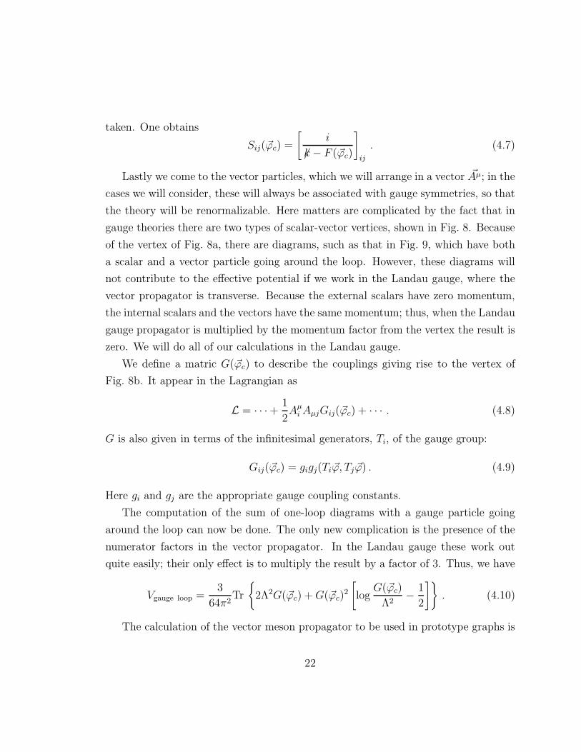
Lastly we come to the vector particles, which we will arrange in a vector ~Aµ; in the
cases we will consider, these will always be associated with gauge symmetries, so that
the theory will be renormalizable. Here matters are complicated by the fact that in
gauge theories there are two types of scalar-vector vertices, shown in Fig. 8. Because
of the vertex of Fig. 8a, there are diagrams, such as that in Fig. 9, which have both
a scalar and a vector particle going around the loop. However, these diagrams will
not contribute to the effective potential if we work in the Landau gauge, where the
vector propagator is transverse. Because the external scalars have zero momentum,
the internal scalars and the vectors have the same momentum; thus, when the Landau
gauge propagator is multiplied by the momentum factor from the vertex the result is
zero. We will do all of our calculations in the Landau gauge.
We define a matric G(~ϕc) to describe the couplings giving rise to the vertex of
Fig. 8b. It appear in the Lagrangian as
L = · · ·+ 1
2Aµ
i AµjGij(~ϕc) + · · · . (4.8)
G is also given in terms of the infinitesimal generators, Ti, of the gauge group:
Gij(~ϕc) = gigj(Ti~ϕ, Tj ~ϕ) . (4.9)
Here gi and gj are the appropriate gauge coupling constants.
The computation of the sum of one-loop diagrams with a gauge particle going
around the loop can now be done. The only new complication is the presence of the
numerator factors in the vector propagator. In the Landau gauge these work out
quite easily; their only effect is to multiply the result by a factor of 3. Thus, we have
Vgauge loop =3
64π2Tr
{
2Λ2G(~ϕc) +G(~ϕc)2
[
logG(~ϕc)
Λ2− 1
2
]}
. (4.10)
The calculation of the vector meson propagator to be used in prototype graphs is
22
also straightforward; one obtains
Dµνij =
i(
−gµν + kµkν
k2
)
k2 −G(~ϕc) + iǫ
ij
. (4.11)
If the vector particles are associated with a non-Abelian gauge group, the the-
ory will also involve fictitious ghost particles7. If one works in the Landau gauge,
the ghosts do not couple to the other scalar particles and therefore need no further
consideration at this point. There will be higher-order graphs contributing to the
effective potential which have ghosts coupled to the gauge particles, but in these the
ghost part of the diagram is calculated as usual. We will see, however, that the ghosts
will complicate the renormalization procedure.
We will not discuss the renormalization procedure in detail at this point, since
it is similar to that for the theory of Chapter III; when appropriate, we will make
some comments in the context of particular theories. Let us now proceed to consider
several models, to see if our methods can detect spontaneous symmetry breaking in
any of them.
1. A Scalar SO(n) Model
This model is very much like our original simple model; instead of a single scalar
fields there are n real fields, transforming as a vector under the group SO(n). The
Lagrangian is
L =1
2∂µ~φ · ∂µ~φ− λ
4!(~φ · ~φ)2 + counter−terms . (4.12)
The effective potential is expected to be a function of the n classical fields. However,
we notice that because of the symmetry of the theory, the effective potential can only
be a function of
ϕ2c =
n∑
k=1
ϕ2kc . (4.13)
Thus we can calculate the effective potential for the case where only ϕ1c is non-zero,
and then immediately extend the results to the general case. In other words, it is
sufficient to calculate only diagrams with external φ1’s. (This is just another way of
saying that the vacuum expectation value of ~φ must point in a particular direction.)
23
We expect two different types of one-loop diagrams: those with a φ1 running around
the loop, and those with one of the other φk’s running around the loop. Referring to
Eqs. (4.1) and (4.2), we see that
U(~ϕc)|ϕ1c 6=0,ϕ2c=ϕ3c=···ϕnc=0 =
12λϕ2
1c 0 · · · 00 1
6λϕ2
1c...
. . .
0 16λϕ2
1c
(4.14)
and thus
V (~ϕc)|ϕ1c 6=0,ϕ2c=ϕ3c=···ϕnc=0 =λ
4!ϕ4
1c +1
64π2
{
2Λ2
(
λ
2+
(n− 1)λ
6
)
ϕ21c
+λ2
4ϕ4
1c
[
logϕ2
1c
2Λ2− 1
2
]
+(n− 1)λ2
36
[
logϕ2
1c
6Λ2− 1
2
]}
+ counter−terms .
(4.15)
We see that there are, as expected, two types of one-loop contributions.
Our renormalization conditions are similar to those of the theory with a single
scalar particle, namely∂2V
∂ϕ21c
∣
∣
∣
∣
∣
ϕ1c=···ϕnc=0
= 0 , (4.16a)
∂4V
∂ϕ41c
∣
∣
∣
∣
∣
ϕ1c=M,ϕ2c=···ϕnc=0
= λ , (4.16b)
and
Z(ϕ1c = M,ϕ2c = · · ·ϕnc = 0) = 1 . (4.16c)
Performing the renormalization, we obtain the final expression for the one-loop ap-
proximation to the effective potential:
V (~ϕ) =λ
4!ϕ4
c +1
64π2
(
λ2
4+
(n− 1)λ2
36
)
ϕ4c
[
logϕ2
c
M2− 25
6
]
. (4.17)
This effective potential is of the same form as that of our previous model, but it
differs from the previous one in having the factor of n − 1 in the logarithmic term.
Thus, we might hope that for sufficiently large n this potential will exhibit a minimum
24
within the range of validity of the one-loop approximation. (In terms of the comments
of the previous chapter, we can attribute this to the presence in this theory of two
types of interactions: the φ4i interaction and the φ2
iφj2 interaction (i 6= j). The
latter first contributes to the effective potential in the one-loop approximation.) If
we differentiate, we obtain, instead of Eq. (3.17),
λ(
1 +n− 1
9
)
(
logϕ2
c
M2− 11
3
)
= −32π2
3. (4.18)
Certainly this equation can be satisfied with both |λ| and | log(ϕ2c/M
2)| being kept
small if n is made sufficiently large; we can obtain a minimum by having many types
of loops, rather than by making a single loop contribution large. Unfortunately,
letting n be large also invalidates the one-loop approximation. For example, consider
the two-loop prototype graphs of the form shown in Fig. 7. Each of the n φk’s can be
allowed to run around the left loop and and each of the n φk’s can be allowed to run
around the right loop; thus there are n2 prototype graphs of this type. Each higher
order will bring in another factor of n, so the L-loop contribution will be of the order
of
λ
(
nλ logϕ2
c
M2
)L
. (4.19)
Thus, if n is large enough to satisfy Eq. (4.18), it is large enough to invalidate the
one-loop approximation. (We see that we were mistaken in identifying two types of
interactions; a better way of describing the theory is to say that it contains a single
many-component field and only one interaction.) This model is no improvement over
our first one.
2. A Yukawa Model
Next we consider a theory with a single scalar field and a single fermion field,
with the Lagrangian
L =1
2∂µφ∂
µφ+ iψ 6∂ψ + igψγ5φψ +λ
4!φ4 + counter−terms . (4.20)
(The quartic scalar self-coupling is required for renormalizability.) Because this the-
ory contains two genuinely distinct interactions, it may be possible to adjust matters
so that the one-loop corrections qualitatively change the nature of the vacuum.
25
Because there is only one scalar field and one fermion field, the matrices U and
F are trivial:
U =1
2λϕ2
c (4.21a)
and
F = igϕcγ5 . (4.21b)
The calculation of the one-loop approximation to the effective potential is straight-
forward; after renormalization one obtains
V =λ
4!ϕ4
c +1
64π2
(
λ2
4− 4g2
)
ϕ4c
[
logϕ2
c
M2− 25
6
]
. (4.22)
Indeed, the Yukawa coupling, which first contributes to the effective potential in
the one-loop approximation, does have an important qualitative effect: The effective
potential has the shape of the previous ones (Fig. 5) only if g4 is less than λ2/16; if
g4 is larger than λ2/16, the effective potential has the shape shown in Fig. 10. The
latter case is clearly unacceptable; the effective potential has no lower bound as the
classical field approaches infinity, so the vacuum does not exist (unless higher-order
contributions make the effective potential turn upward, but in that case the one-loop
approximation is still useless). And the former case has the same difficulties as our
earlier models, but to a greater degree: the minimum is even further from the region
of validity of the one-loop approximation. Thus, we have found a theory where the
one-loop contribution to the effective potential has an important qualitative effect;
unfortunately, it isn’t the sort of effect we were looking for.
3. Massless Scalar Electrodynamics
Now we consider the theory of two real (or one complex) scalar fields coupled to
a gauge vector meson, with the Lagrangian
L =1
4F µνFµν +
1
2(∂µφ1 − eAµφ2)
2 +1
2(∂µφ2 + eAµφ1)
2 − λ
4!(φ2
1 + φ22)
2
+ counter−terms ,(4.23)
where
F µν = ∂νAµ − ∂µAν . (4.24)
26
If this theory has a symmetric vacuum, it describes the electrodynamics of a massless
charged scalar meson. If spontaneous symmetry breaking occurs, then by the usual
Higgs mechanism we obtain the theory of a single massive scalar meson coupled to
a massive vector meson. To determine which is the case is to determine whether
the infrared divergences associated with massless charged scalar particles are strong
enough to prevent such particles from existing.
The calculation of the one-loop approximation to the effective potential is straight-
forward, as is the renormalization; one obtains
V =λ
4!ϕ4
c +1
64π2
(
λ2
4+λ2
36+ 3e4
)
ϕ4c
[
logϕ2
c
M2− 25
6
]
. (4.25)
where
ϕ2c = ϕ2
1c + ϕ22c . (4.26)
This effective potential also has the shape shown in Fig. 5; it appears to have a
minimum at a non-zero value of ϕc. We again must determine whether the minimum
occurs within the range of validity of the one-loop approximation. We can simplify
our equations if we recall that M is an arbitrary parameter; we are certainly allowed
to choose M to be the location of the minimum of the effective potential, 〈φ〉. We
finddV
dϕc
∣
∣
∣
∣
∣
ϕc=M=〈φ〉
=λ
6〈φ〉3 +
1
64π2
(
λ2
4+λ2
36+ 3e4
)
(
−44
3〈φ〉2
)
. (4.27)
Thus, we must see if we can satisfy
λ =11
8π2
(
3e4 +λ2
4+λ2
36
)
(4.28)
while keeping both e and λ small enough that our approximation is valid. Clearly we
can do this if we choose λ to be of the order of e4. If we do this, we should ignore the
λ2 terms, since they are of the same order of magnitude as the e8 terms we expect
from two-loop diagrams. Thus, in the one-loop approximation we find that if
λ =33e4
8π2, (4.29)
27
there will be a minimum in the effective potential which is within the region where the
approximation is valid. The gauge coupling, which only contributes to the effective
potential through loop diagrams, has caused spontaneous symmetry breaking.
If we substitute Eq. (4.29) back into Eq. (4.25), we obtain
V =3e4
64π2ϕ4
c
[
logϕ2
c
〈φ〉2 − 1
2
]
. (4.30)
All reference to the parameter λ has disappeared from the effective potential. Note
that even if we had chosen to define λ differently (for example, by using Eq. (3.11b)),
we would have obtained different results for Eqs. (4.25-29), but the same result for
Eq. (4.30).
At first glance, a very strange thing seems to have occurred: Starting with two
dimensionless parameters, e and λ, we have obtained a theory with one dimensionless
parameter, e, and one dimensional parameter, 〈φ〉. Furthermore, the dependence on
〈φ〉 is trivial, being determined solely by dimensional considerations. A little thought
will make this seem less strange. Originally, the theory was really characterized by
three parameters: e, λ, and M ; however, one two of these were independent and the
dependence on M was not explicitly shown. The final description of the theory is
also characterized by three parameters: e, 〈φ〉, and 〈φ〉/M ; again only two are truly
independent, and we have not shown the dependence on the third parameter, which
we have set equal to one. Of course, we could have renormalized at a point other than
the minimum of the effective potential (that is, with 〈φ〉/M 6= 1), and would have
obtained a different expression for the effective potential and a different relationship
between λ and e, although the physics would have been the same. In other words,
both descriptions contain two dimensionless and one dimensional parameters, with
only two being truly independent. The difference between the two descriptions is that
in the second one dimensional analysis tells us a great deal; there is a two-parameter
family of spontaneously broken theories, but changing one of the parameters, 〈φ〉, is
completely equivalent to changing the scale in which masses are measured, so that
effectively there is only a one-parameter family.
Another important point is the singularity in the effective potential (and thus
28

in the effective action) at ϕc = 0. Because of this branch point, we cannot expand
the effective action in a Taylor series about ϕc = 0; the expansion in terms of the
n-point IPI Green’s functions is not valid. If it were, we could approximate the
effective potential near ϕc = 0 (although not everywhere) by the sum of the first few
Green’s functions. It isn’t, and therefore we must do an infinite sum even to get an
approximation to the effective potential.
Even if we had taken the theory at face value, as massless scalar electrodynamics,
there would not have been a simple interpretation of the Green’s functions in terms
of S-matrix elements, because of the presence of massless particles. To calculate any
physical process we would have had to sum over sets of degenerate states with various
numbers of particles at infinitesimal momenta.
At this point, we can transform the fields as is usually done in Higgs models to
obtain a massive scalar field and a massive vector field. If we define these masses in
terms of the values of the inverse propagators at zero momentum, we obtain
m2(S) =d2V
dϕ2c
∣
∣
∣
∣
∣
ϕc=〈φ〉
=3e4
8π2〈φ〉2 (4.31)
and
m2(V ) = e2〈φ〉2 (4.32)
and thusm2(S)
m2(V )=
3e2
8π2=
3
2πα . (4.33)
It is important to remember that the expression we have obtained for the effective
potential is only valid in the region of classical field space where log(ϕ2c/M
2) is small;
in other words, it is not valid for very large or very small ϕc. Thus, there might
be deeper minima than the one we have found, which lie in regions inaccessible to
our computational methods. However, the value of the effective potential at the
origin will remain zero, even if higher-order effects cause this to be a minimum rather
than the maximum which the one-loop approximation indicates. Since the effective
potential is negative at the minimum which we have found, and since this minimum
is in a region where higher-order effects are expected to be small, we see that the
29
absolute minimum cannot occur at the origin; spontaneous symmetry breaking occurs
for small values of e, at least when λ is of the order of e4.
4. Other Gauge Theories
The results for a more complicated (possibly non-Abelian) gauge theory contain-
ing many spin-0 and spin-1/2 particles are, in general, qualitatively similar to those
for scalar electrodynamics. First, we note that in these theories the matrices U(ϕc),
F (ϕc) andG(ϕc) have a simple physical interpretation: when evaluated at the vacuum
expectation value of φ, they are the zero-loop approximations to the mass matrices
of the spin-0, spin-1/2, and spin-1 particles, respectively. If the vector meson masses
are sufficiently larger than those of the scalar mesons and fermions, the effects of the
scalar and fermion loops will be negligible compared to those of the vector loops.
(Remember that the contribution of the loop diagrams is roughly proportional to the
fourth power of the relevant mass.) In this case, we obtain
V = V0(ϕc) +3e4
64π2Tr
{
G(ϕc)2
[
logG(ϕc)
M2− 25
6
]}
(4.34)
as the one-loop approximation to the effective potential. If there is a single mul-
tiplet of scalar particles whose self-interactions are described by a single quartic
self-coupling, we can absorb V0 into the vector loop by replacing M by µ, where
µ, unlike M , is not arbitrary, since its value determines the strength of the scalar
self-interaction. We can then write
V =3e4
64π2Tr
{
G(ϕc)2
[
logG(ϕc)
µ2− 1
2
]}
. (4.35)
This equation is of the same form as Eq. (4.30); we expect it to have the same
consequences: a minimum in the effective potential, which gives rise to spontaneous
symmetry breaking and a single relationship among masses. Otherwise, we expect
theories with our mass renormalization condition to be similar to the more usual
ones with a negative mass term; by adding one restriction, we have obtained one new
result.
To illustrate all this, we consider the Weinberg-Salam model of leptons,8 modified
by requiring that the scalar mass term in the Lagrangian vanish. This model is
30
based on an SU(2)×U(1) gauge symmetry; the gauge fields are denoted by ~W µ and
Bµ, with coupling constants g and g′, respectively. There is a single complex scalar
doublet; with no loss of generality, we can assume that only the real part of one of
its components has a non-zero vacuum expectation value. Because the leptons are
light, their effects on the effective potential can be neglected. We assume that the
final massive scalar meson is light enough that the scalar loop contributions can also
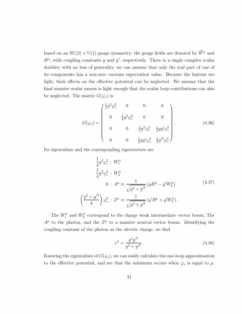
be neglected. The matric G(ϕc) is
G(ϕc) =
14g2ϕ2
c 0 0 0
0 14g2ϕ2
c 0 0
0 0 14g2ϕ2
c14gg′ϕ2
c
0 0 14gg′ϕ2
c14g′2ϕ2
c
. (4.36)
Its eigenvalues and the corresponding eigenvectors are
1
4g2ϕ2
c : W µ1
1
4g2ϕ2
c : W µ2
0 : Aµ ≡ 1√
g2 + g′2(gBµ − g′W µ
3 )
(
g2 + g′2
4
)
ϕ2c : Zµ ≡ 1
√
g2 + g′2(g′Bµ + g′W µ
3 ) .
(4.37)
The W µ1 and W µ
2 correspond to the charge weak intermediate vector boson, The
Aµ to the photon, and the Zµ to a massive neutral vector boson. Identifying the
coupling constant of the photon as the electric charge, we find
e2 =g2g′2
g2 + g′2. (4.38)
Knowing the eigenvalues of G(ϕc), we can easily calculate the one-loop approximation
to the effective potential, and see that the minimum occurs when ϕc is equal to µ.
31
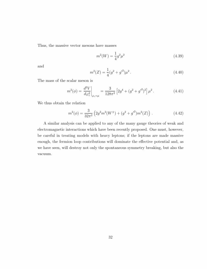
Thus, the massive vector mesons have masses
m2(W ) =1
4g2µ2 (4.39)
and
m2(Z) =1
4(g2 + g′
2)µ2 . (4.40)
The mass of the scalar meson is
m2(φ) =d2V
dϕ2c
∣
∣
∣
∣
∣
ϕc=µ
=3
128π2
[
2g4 + (g2 + g′2)2]
µ2 . (4.41)
We thus obtain the relation
m2(φ) =3
32π2
(
2g2m2(W±) + (g2 + g′2)m2(Z)
)
. (4.42)
A similar analysis can be applied to any of the many gauge theories of weak and
electromagnetic interactions which have been recently proposed. One must, however,
be careful in treating models with heavy leptons; if the leptons are made massive
enough, the fermion loop contributions will dominate the effective potential and, as
we have seen, will destroy not only the spontaneous symmetry breaking, but also the
vacuum.
32
V. Massive Theories
So far, we have restricted ourselves to the consideration of theories in which the
Lagrangian does not contain a mass term; we will now remove that restriction and
consider theories in which mass terms (either positive or negative) are present. The
models we have considered previously are special cases of this large class of theo-
ries — special not because they contain massless particles (they don’t necessarily),
but because their only dimensional parameter is the renormalization point, which
is arbitrary and which can be changed without affecting the physics. While this is
significant, it does not seem to be the sort of property that should characterize the
transition point between normal theories and spontaneously broken ones. Therefore,
we might expect quantum corrections to invalidate the conventional wisdom — per-
haps there are theories which are spontaneously broken even though the Lagrangian
contains a positive mass-squared, or theories which have a negative mass-squared in
the Lagrangian and yet have a symmetric vacuum. We shall study a few models to
see if we can find any.
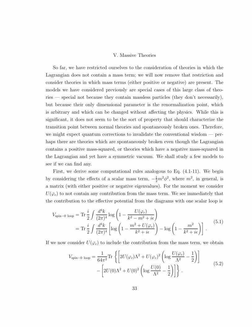
First, we derive some computational rules analogous to Eq. (4.1-11). We begin
by considering the effects of a scalar mass term, −12m2φ2, where m2, in general, is
a matrix (with either positive or negative eigenvalues). For the moment we consider
U(ϕc) to not contain any contribution from the mass term. We see immediately that
the contribution to the effective potential from the diagrams with one scalar loop is
Vspin−0 loop = Tri
2
∫ d4k
(2π)4log
(
1 − U(ϕc)
k2 −m2 + iǫ
)
= Tri
2
∫
d4k
(2π)4
[
log
(
1 − m2 + U(ϕc)
k2 + iǫ
)
− log
(
1 − m2
k2 + iǫ
)]
.
(5.1)
If we now consider U(ϕc) to include the contribution from the mass term, we obtain
Vspin−0 loop =1
64π2Tr
{[
2U(ϕc)Λ2 + U(ϕc)
2
(
logU(ϕc)
Λ2− 1
2
)]
−[
2U(0)Λ2 + U(0)2
(
logU(0)
Λ2− 1
2
)]}
.
(5.2)
33

The second term is constant in classical field space; its only role it to assure that
the effective potential vanishes when ϕc = 0. The scalar propagator to be used in
prototype graphs is even simpler to calculate; clearly, Eq. (4.3) remains true if U(ϕc)
is interpreted to include the mass term contributions. The rules for spin-1/2 and
spin-1 fields are just as simple. F (ϕc) and G(ϕc) are now understood to include con-
tributions from the appropriate mass terms. The formulas for the propagators remain
unchanged, while the rules for calculating the one-loop contributions are altered only
by the subtraction of the value of the loop at ϕc = 0.
After renormalization, however, the expression for the effective potential becomes
more complicated than previously; this is a consequence of the fact that U(ϕc),
F (ϕc), and G(ϕc) are more complicated functions of ϕc than before, which makes
the derivatives of V (ϕc) more complicated also.
1. Massive λφ4 Theory
We return to our original model, adding a mass term. The Lagrangian is now
L =1
2(∂µφ)2 − 1
2m2φ2 − λ
4!φ4 + counter−terms (5.3)
The renormalization conditions we impose are
d2V
dφ2c
∣
∣
∣
∣
∣
ϕc=0
= m2 , (5.4)
d4V
dϕ4c
∣
∣
∣
∣
∣
ϕc=M
= λ , (5.5)
and
Z(M) = 1 . (5.6)
Notice that we have retained the arbitrary non-zero renormalization point, even
though there is no singularity at ϕc = 0 when m2 6= 0. The reason should be clear; if
we want to consider our previous model as a special case of a more general class, we
should impose the same renormalization conditions throughout. (Although M is still
arbitrary, the dependence of the effective potential on M is no longer determined by
dimensional analysis, since the theory now contains a second dimensional parameter.)
34

First, we consider the case where both m2 and λ are positive. A straightforward
(but agonizing) calculation yields
V =m2
2ϕ2
c +λ
4!ϕ4
c +1
64π2
(
m2 +λϕ2
c
2
)2
log
(
1 +12λϕ2
c
m2
)
− 1
64π2
1
2m2λϕ2
c +λ2ϕ4
c(
m2 + 12λM2
)2
(
3
8m4 +
7
8m2λM2 +
25
96λ2M4
)
]
− λ2ϕ4c
256π2log
(
m2 + 12λM2
m2
)
.
(5.7)
The effective potential vanishes at the origin, as it should. We note that the first
three terms are always non-negative, while the terms in square brackets, which are
negative, are negligible unless λ is large (of the order of 64π2). Only the last term
can make the effective potential turn negative, which evidently will happen if 12λM2
is much greater than m2. Of course, this will put the minimum at a small value of
ϕc/M (but with λϕ2c > m2), which is outside the region of validity of the one-loop
approximation, but we do see our previous results, for m2 = 0, emerging as the limit
of the massive ones.
Now we let m2 be negative, and write m2 = −µ2. We obtain
V = −µ2
2ϕ2
c +λ
4!ϕ4
c +1
64π2
(
−µ2 +λϕ2
c
2
)2
log
(
|µ2 − 12λϕ2
c |µ2
)
+1
64π2
1
2λµ2ϕ2
c +λ2ϕ4
c(
µ2 − 12λM2
)2
(
−3
8µ4 +
7
8λµ2M2 − 25
96λ2M4
)
]
− λ2ϕ4c
256π2log
(
|µ2 − 12λM2|
µ2
)
+i
64π
(
λϕ2c
2− µ2
)2
θ
(
µ2 − λϕ2c
2
)
− µ4
.
(5.8)
Postponing for a moment the discussion of the imaginary part, let us investigate
the behavior of the real part of the effective potential as µ2 is varied while 12λM2
is held fixed. There is a singularity at µ2 = 12λM2, but the one-loop approximation
clearly fails near this point, since additional loops will bring in additional factors of
35
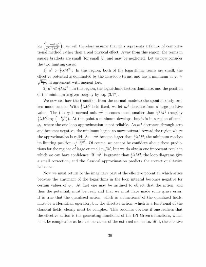
log(
µ2− 1
2λϕ2
c
µ2− 1
2λM2
)
; we will therefore assume that this represents a failure of computa-
tional method rather than a real physical effect. Away from this region, the terms in
square brackets are small (for small λ), and may be neglected. Let us now consider
the two limiting cases:
1) µ2 > 12λM2 : In this region, both of the logarithmic terms are small; the
effective potential is dominated by the zero-loop terms, and has a minimum at ϕc ≈√
6µ2
λ, in agreement with ancient lore.
2) µ2 ≪ 12λM2 : In this region, the logarithmic factors dominate, and the position
of the minimum is given roughly by Eq. (3.17).
We now see how the transition from the normal mode to the spontaneously bro-
ken mode occurs: With 12λM2 held fixed, we let m2 decrease from a large positive
value. The theory is normal unit m2 becomes much smaller than 12λM2 (roughly
12λM2 exp
(
−8π2
3λ
)
). At this point a minimum develops, but it is in a region of small
ϕc, where the one-loop approximation is not reliable. As m2 decreases through zero
and becomes negative, the minimum begins to move outward toward the region where
the approximation is valid. As −m2 become larger than 12λM2, the minimum reaches
its limiting position,√
−6m2
λ. Of course, we cannot be confident about these predic-
tions for the regions of large or small ϕc/M , but we do obtain one important result in
which we can have confidence: If |m2| is greater than 12λM2, the loop diagrams give
a small correction, and the classical approximation predicts the correct qualitative
behavior.
Now we must return to the imaginary part of the effective potential, which arises
because the argument of the logarithms in the loop integral becomes negative for
certain values of ϕc. At first one may be inclined to object that the action, and
thus the potential, must be real, and that we must have made some grave error.
It is true that the quantized action, which is a functional of the quantized fields,
must be a Hermitian operator, but the effective action, which is a functional of the
classical fields, clearly must be complex. This becomes obvious if one realizes that
the effective action is the generating functional of the IPI Green’s functions, which
must be complex for at least some values of the external momenta. Still, the effective
36

potential will normally remain real, since the imaginary part corresponds to on-shell
intermediate states, which normally cannot be produced if all the external momenta
vanish. However, if the theory contains a particle with imaginary mass, on-shell
intermediate states can be produced, even though the external momenta vanish. Of
course, the theory doesn’t really contain any particles with imaginary mass, but
we are doing perturbation theory as if it did, and the Green’s functions only have
meaning in the context of a particular perturbation theory; if we redefine the fields
so as to eliminate the appearance of a negative mass-squared, the Green’s functions
are correspondingly redefined, and have no simple relation to the previously defined
ones. (Since we are assuming that the potential is unchanged by a redefinition of
the fields, we must conclude that the imaginary part vanishes when calculated to all
orders; this does not forbid its presence to any finite order.)
Having convinced ourselves that the imaginary part of the effective potential is not
nonsense, we must see how matters are altered by its presence. Since the quantized
action, and thus the counter-terms, must be real, we can only renormalize the real
part of the effective action; that is, we require that
d2(ReV )
dφ2c
∣
∣
∣
∣
∣
ϕc=0
= −µ2 (5.9)
andd4(ReV )
dφ4c
∣
∣
∣
∣
∣
ϕc=M
= λ . (5.10)
(This was done in obtaining Eq. (5.8).) We note that the imaginary part is finite, even
without being renormalized. Also, we looked for spontaneous symmetry breaking by
searching for the minimum of the real part of the effective potential, but this does
not matter; for the imaginary part has two terms, of which one is independent of ϕc,
and thus physically meaningless, while the other vanishes unless ϕc <√
2µ2
λ, which is
always below the neighborhood of the minimum.
So far, we have been assuming that λ is positive; what happens when λ is negative? In
this case, the zero-loop approximation to the effective potential has no lower bound.
It is possible that the contributions from diagrams with one or more loops might
37
make the effective potential turn upward at large ϕc (as the one-loop terms appear to
do), but our approximation cannot determine this. Later we shall see how to improve
our approximation, and will find that this does not happen. In any case, there is no
minimum within the region of validity of our approximation, no matter what the sign
of m2.
2. Massive Scalar Electrodynamics
Next we turn to massive scalar electrodynamics, described by the Lagrangian
L =1
4F µνFµν +
1
2(∂µφ1 − eAµφ2)
2 +1
2(∂µφ2 + eAµφ1)
2
− 1
2m2(φ2
1 + φ22) −
λ
4!(φ2
1 + φ22)
2 + counter−terms .
(5.11)
If λ is much greater than e4, we expect that the contributions to the effective potential
from scalar loop diagrams will dominate those from photon loop diagrams and that
the effective potential will behave qualitatively like that of the λφ4 theory. Therefore,
let us assume that λ is of the order of e4, or smaller. In the one-loop approximation,
we should then neglect the scalar loop diagrams, since they are of the same order
of magnitude as the diagrams with two photon loops. We obtain for the effective
potential
V =1
2m2ϕ2
c +λ
4!ϕ4
c +3e4
64π2ϕ4
c
(
logϕ2
c
M2− 25
6
)
. (5.12)
Here M is, as usual, the value of ϕc at which the renormalizations are done. There
is no restriction on the sign of either m2 or λ.
Now we define a quantity µ, with the dimensions of mass, by
λ
4!=
3e4
64π2
(
logM2
µ2+
11
3
)
. (5.13)
We then obtain
V =1
2m2ϕ2
c +3e4
64π2ϕ4
c
(
logϕ2
c
µ2− 1
2
)
. (5.14)
Note that µ, unlike M , is not arbitrary; Eq. (5.14) does not contain any redundant
parameters. We see that µ is the position of the minimum if m2 vanishes.
38
To study the behavior of the effective potential, we will need the following equa-
tions:dV
dϕc= ϕc
(
m2 +3e4µ2
16π2
ϕ2c
µ2log
ϕ2c
µ2
)
, (5.15)
d4V
dϕ4c
=9e4
8π2
(
logϕ2
c
µ2+
11
3
)
. (5.16)
It will also be useful to consider the behavior of the function f(x) = x log(x), shown
in Fig. 11.
We begin by considering the case of positive m2. We see that there is a minimum
at the origin, but that if m2 is sufficiently small, the effective potential will have
a second minimum arising from the logarithmic term; the situation will be as in
either Fig. 12a or Fig. 12b. To determine matters more quantitatively, we consider
Eq. (5.15), and see that the condition for an extremum away from the origin is
m2 = −3e4µ2
16π2f
(
ϕ2c
µ2
)
. (5.17)
If m2 > 3e4µ2
16π2 e−1, Eq. (5.17) cannot be satisfied; the effective potential behaves as
in Fig. 12c. If 0 < m2 < 3e4µ2
16π2 e−1, there will be two solutions, one for ϕ2
c/µ2 < e−1
and one for ϕ2c/µ
2 > e−1. Clearly the former corresponds to a maximum and the
latter to a minimum. We must now determine whether this is an absolute minimum.
The effective potential vanishes at the origin; From Eqs. (5.14) and (5.17) we see that
at ϕ2c/µ
2 = β it is
V (βµ2) =βµ4
4
(
m2 − 3e4µ2
32π2β
)
. (5.18)
The condition for an absolute minimum away from the origin is therefore
β >32π2m2
3e4µ2, (5.19)
where β satisfies
β log β = −16π2m2
3e4µ2. (5.20)
After a little algebra, we see that this condition is satisfied if β > e−1/2. Thus, there
three regions:
39

1) 0 < m2 < 3e4µ2
32π2 e−1/2 : The effective potential behaves as in Fig. 12a; sponta-
neous symmetry breaking occurs.
2) 3e4µ2
32π2 e−1/2 < m2 < 3e4µ2
16π2 e−1 : The effective potential behaves as in Fig. 12b; the
vacuum is symmetric.
3) m2 > 3e4µ2
16π2 e−1 : The effective potential behaves as in Fig. 12c; again there is
no spontaneous symmetry breaking.
The results for region (1) seem in contradiction with the conventional wisdom
— they predict spontaneous symmetry breaking for a theory with a positive mass-
squared. To show that there is no contradiction, we calculate λ, using Eq. (5.16):
λ =d4V
dϕ4c
∣
∣
∣
∣
∣
ϕc=M
=9e4
8π2
(
logM2
µ2+
11
3
)
. (5.21)
Normally, we would choose M to be of the order of magnitude of m, since m is the
only dimensional parameter in the initial formulation of the theory. (It is true that
there is another dimensional parameter, the position of the minimum of the effective
potential, which is much greater than m, but this is not originally evident.) If we
choose M ≈ m, and let m2 be in region (1), we find that λ is negative (unless e4
is absurdly large). This is not the theory of which the conventional wisdom speaks;
instead, it is one which is usually discarded as not having a lower bound on the
effective potential. However, we see that the effect of the quantum corrections is to
make the effective potential turn upward at large ϕc, and thus remedy the situation.
To obtain the more usual theory, with a positive λ, m2 must be in either region (2)
or region (3), where the vacuum is, in fact, symmetric.
Now we turn to the case of negative m2. There is a maximum at the origin, and
a minimum determined by
f
(
ϕ2c
µ2
)
=ϕ2
c
µ2log
ϕ2c
µ2= −16π2m4
3e4µ2=
16π2
3e4µ2|m2| . (5.22)
We see from Fig. 11 that this equation has only one solution. For |m2| ≪ µ2, this
solution is at ϕc ≈ µ, which is in agreement with our results for m2 = 0. In general,
the minimum occurs when
|m2| =3e4
16π2ϕ2
c logϕ2
c
µ2. (5.23)
40
To determine the mass of the scalar particle, we calculate
m2(φ) =d2V
dϕ2c
∣
∣
∣
∣
∣
ϕc=〈φ〉
= −m2 +3e4
16π2〈φ〉2
(
3 log〈φ〉2µ2
+ 2
)
= 2|m2| + 3e4
8π2〈φ〉2 .
(5.24)
The first term is the usual (zero-loop) result for modes of this type, while the second
term is just our result for the case of m2 = 0. As λ (defined at the minimum of the
effective potential) is increased above e4, we find that
〈φ〉2 ≈ 6|m2|λ
(5.25)
and
m2(φ) = 2|m2|(
1 +9e4
8π2λ
)
. (5.26)
For λ much greater than e4, the second term on the right hand side of Eq. (5.26) is
negligible, and the classical result holds.
3. Electrodynamics with Massive Photons
A model which is useful for understanding the physical principals behind our
results is the theory of a massive charged scalar meson coupled to a massive photon.9
If we assume that the scalar quartic coupling constant, λ, is of the order of e4, we
need only consider diagrams with photon loops in the one-loop approximation. The
expression we obtain for the effective potential is
V =λ
4!ϕ4
c +3
64π2
{
(m2 + e2ϕ2c) log
(
1 +e2ϕ2
c
m2
)
− e2ϕ2cm
2
− e4ϕ4c
(m2 + e2M2)2
(
3
2m4 + 7e2m2M2 +
25
6e4M4
)
+e4ϕ4c log
(
m2
m2 + e2M2
)}
,
(5.27)
where M is the value of ϕc at which λ is defined and m is the mass of the photon.
We see that if m2 is much larger than e2M2, the effective potential does not possess
41
a minimum away from the origin. In other words, the coupling to the photon can
produce spontaneous symmetry breaking only if the photon is sufficiently light. But
this is equivalent to saying that spontaneous symmetry breaking occurs only if the
range of the electromagnetic interaction is sufficiently long. This agrees with physical
intuition, since spontaneous symmetry breaking is essentially a correlation of the field
through all of space, which should require long-range forces. It is true that long-range
forces are not evident in the usual examples of the Goldstone phenomenon, where
spontaneous symmetry breaking is induces by a negative mass-squared term in the
Lagrangian, but this is such an unnatural term that we really don’t have any physical
interpretation for it until we redefine the fields. (And when we do redefine the fields,
we obtain massless particles, and thus long-range forces.)
4. A Model with Pseudo-Goldstone Bosons
Finally we consider a model in which the quantum corrections must be consid-
ered in order to completely determine the character of the vacuum, even though the
Lagrangian contains a negative mass-squared term. The model is based on an SU(3)
gauge symmetry; in addition to the gauge vector mesons, it has an octet of spinless
mesons, φ, which we write as a 3 × 3 traceless Hermitian matrix. If we impose the
requirement that the Lagrangian be invariant under the transformation φ→ −φ, the
most general form for the non-derivative scalar meson terms in the Lagrangian is
Lscalar = −µ2Trφ2 + a(
Trφ2)2
+ bTrφ4 . (5.28)
However, we note that for three-dimensional traceless Hermitian matrices
Trφ4 =1
2
(
Trφ2)2. (5.29)
Thus the zero-loop approximation so the effective potential is of the form
V0 = −µ2Trφ2 + λ(
Trφ2)2. (5.30)
We note that this expression involves only Tr(φ2), which is invariant under the trans-
formations of SO(8); minimizing it will determine only Tr(φ2), but not Det(φ), which
42

is an invariant under SU(3) transformations but not under SO(8) transformations.
Yet, because of the presence of the vector mesons and their couplings to the scalar
mesons, the Lagrangian is invariant only under SU(3), and not under SO(8). There-
fore, we must calculate the one-loop contributions to the effective potential, where
the effects of the vector mesons first appear, in order to completely determine the
nature of the spontaneous symmetry breaking.
The SO(8) invariance of the zero-loop effective potential has another important
consequence: The spontaneous breaking of SO(8) symmetry gives rise to a single
massive scalar and seven massless Goldstone bosons; we will obtain the same result
in the zero-loop approximation to our model, since to that order our model is the
same as an SO(8) symmetric one. However, when SU(3) is spontaneously broken,
either SU(2)×U(1) or U(1)×U(1) remains as an unbroken subgroup; only four or six
of the Goldstone bosons can be eaten by the vector meson through the Higgs-Kibble
mechanism. The remaining massless bosons acquire a mass when loop effects are
included; they are only pseudo-Goldstone bosons.10
The most general form for the vacuum expectation value of φ can be written as
〈φ〉 =
a 0 00 b 00 0 c
, a + b+ c = 0 . (5.31)
If a = b (or a = c, etc.), there will be an unbroken SU(2)×U(1) subgroup; otherwise
the unbroken subgroup will be U(1)×U(1). We assume that the vector meson masses
are enough larger than those of the scalar mesons that only the contribution to the
effective potential from the vector meson loops is important. The matrix G(〈φ〉) is
43
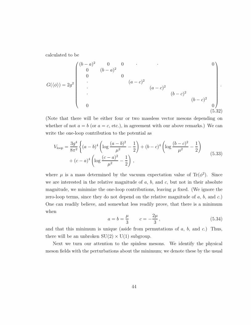
calculated to be
G(〈φ〉) = 2g2
(b− a)2 0 0 · · 00 (b− a)2
0 0· (a− c)2
· (a− c)2
· (b− c)2
(b− c)2
0 0
.
(5.32)
(Note that there will be either four or two massless vector mesons depending on
whether of not a = b (or a = c, etc.), in agreement with our above remarks.) We can
write the one-loop contribution to the potential as
Vloop =3g4
8π2
{
(a− b)4
(
log(a− b)2
µ2− 1
2
)
+ (b− c)4
(
log(b− c)2
µ2− 1
2
)
+ (c− a)4
(
log(c− a)2
µ2− 1
2
)
,
(5.33)
where µ is a mass determined by the vacuum expectation value of Tr(φ2). Since
we are interested in the relative magnitude of a, b, and c, but not in their absolute
magnitude, we minimize the one-loop contributions, leaving µ fixed. (We ignore the
zero-loop terms, since they do not depend on the relative magnitude of a, b, and c.)
One can readily believe, and somewhat less readily prove, that there is a minimum
when
a = b =µ
3c = −2µ
3, (5.34)
and that this minimum is unique (aside from permutations of a, b, and c.) Thus,
there will be an unbroken SU(2) × U(1) subgroup.
Next we turn our attention to the spinless mesons. We identify the physical
meson fields with the perturbations about the minimum; we denote these by the usual
44

notation for the pseudoscalar octet. These are related to diagonal perturbations by
a =µ
3+
1√2π0 +
1√6η ,
b =µ
3− 1√
2π0 +
1√6η ,
c = −2µ
3− 2√
6η .
(5.35)
Substituting this into Eq. (5.33), we find
∆m2(π0) =3g4µ2
π2(5.36)
and
∆m2(η) =9g4µ2
π2, (5.37)
where ∆m2 indicates the contribution of the one-loop terms to the scalar meson
masses. Since isospin is an unbroken symmetry, the results for the π+ and π− must
be the same as that for the π0. Furthermore, since there are only four massive scalars,
the K’s must all be Goldstone bosons, which are eaten by the four vector mesons
which become massive. Finally, we note that the η is clearly the meson which acquired
a mass in zeroth order; the pions are the pseudo-Goldstone bosons, and their entire
mass is given by Eq. (5.36).
Now we use Eqs. (5.32) and (5.34) to obtain the vector meson masses; we find
that the four massive vector mesons have a mass given by
m2(V ) = 2g2µ2 . (5.38)
We thus have the relationshipm2(π)
m2(V )=
3g2
2π2. (5.39)
45
VI. The Renormalization Group
In this chapter we show that for the class of theories in which the Lagrangian does
not contain any masses (or any other dimensional parameters) it is possible to improve
the one-loop approximation to the effective potential by the use of renormalization
group methods.11 Recall that the validity of the one-loop approximation required
that both the coupling constants and the logarithms (e.g., log(ϕ2c/M
2)) be small.
However, these are not two completely independent conditions; M is arbitrary in that
a variation of M can be compensated for by a suitable variation of other quantities
in the theory, leaving the physics unchanged. For this to be so, it is clear that
the dependence of the effective action on the coupling constants and on M must be
intertwined. The nature of the interdependence is most easily determined in theories
which contain no dimensional parameter other than M , for in these the dependence
on M is determined by dimensional analysis.
To formulate these considerations more exactly, let us consider a theory with n
coupling constants λi and m fields ψj . The ψj include all fields, regardless of their
spin. The statement that a variation of M can be compensated for by a variation of
the λi and of the normalization of the ψj is
0 =
M∂
M+∑
i
βi(λ)∂
λi+∑
j
γj(λ)∫
d4xψcj(x)δ
δψcj(x)
Γ , (6.1)
where Γ is the effective action. The βi and the γj can be functions of only the λi, since
there are no other dimensionless parameters available. If we apply this equation to
the expansion of Γ in terms of the IPI Green’s functions, we obtain the usual equation
of the renormalization group. However, as we have said before, this is not the best
expansion for our purposes. Instead, we work with the Taylor series expansion of Γ.
Since each term in this expansion is identified by the power of momentum and the
number of fields with spin, the action of the differential operator of Eq. (6.1) does
not mix terms, and so Eq. (6.1) must hold term by term. Let us specialize to the
case where there is only a single spinless field φ(x), which we have now expanded
about Φc(x) = ϕc, and any number of fields with spin. (The results are unchanged
46

if we replace the single spinless field by an SO(n) vector of spinless fields.) A typical
term in our expansion of Γ will contain nj fields of type j (possibly including Φc(x)),
some power of momentum, and a dimensionless function F (ϕc, λi,M). Analogous to
Eq. (6.1), we will obtain
M∂
M+∑
i
βi(λ)∂
λi
+∑
j
(nj γj(λ)) + ϕc∂
ϕc
F (ϕc, λi,M) (6.2)
Now we use the fact that M is the only dimensional parameter in the theory; di-
mensional analysis tells us that F can be a function of only ϕc/M and the λi. If we
define
t = logϕc
M, (6.3)
βi =βi
1 − γϕ, (6.4)
and
γj =γj
1 − γϕ, (6.5)
we can rewrite Eq. 6.2) as
− ∂
∂t+∑
i
βi(λ)∂
λi
+∑
j
njγj(λ)
F (t, λ) . (6.6)
Assuming that we know the βi and the γj , we can write down the general solution to
Eq. (6.6).12 It is
F (t, λ) = f(λ′(t, λ)) exp∫ t
0dt′∑
j
njγj(λ′(t′, λ)) , (6.7)
where λ′i(t, λ) is determined by
∂λ′i(t, λ)
∂t= βi(λ
′) (6.8)
and
λ′i(0, λ) = λi (6.9)
47
and f is an arbitrary function of λ′.
These equations are very pretty, but they involve the βi and the γj, which we
don’t know until we have solved the theory exactly, at which point we don’t need the
equations. However, our perturbation method allows us to obtain approximations for
the βi(λ′) and the γj(λ
′) which are valid for small λ′: We use the one-loop calculations
to obtain βi(λ′(0, λ)) and γj(λ
′(0, λ)), and then use Eq. (6.8) to obtain an expression
for λ′i(t, λ) which is valid in that range of t where λ′ remains small. What we have
gained in comparison with our previous method is that λ′ may remain small even
when t is large, so that our new results will be valid in this region, even though our
old ones were not. Let us now demonstrate the application of these methods to some
models.
1. λφ4 Theory
Because of its simplicity, we return to our original model. In this section we
modify it slightly by choosing Eq. (3.11b) as the coupling constant renormalization
condition. We can then define a function U(t, λ) by
V (ϕc) =ϕ4
c
4!U(t, λ) . (6.10)
Our coupling constant and wave function renormalization conditions are then
U(0, λ) = λ (6.11)
and
Z(λ) = 1 . (6.12)
If we substitute Z(t, λ) and U(t, λ) for F (t, λ) in Eq. (6.6), and evaluate at t = 0,
we obtain
− ∂Z
∂t
∣
∣
∣
∣
∣
t=0
+ 2γ(λ) = 0 (6.13)
and
− ∂U
∂t
∣
∣
∣
∣
∣
t=0
+ β(λ) + 4λγ(λ) = 0 . (6.14)
48

Furthermore, we can substitute Z(t, λ) and U(t, λ) for F (t, λ) in Eq. (6.7), again
evaluate at t = 0, and obtain
Z(0, λ) = 1 = fZ(λ′(0, λ) = fZ(λ) (6.15)
and
U(0, λ) = λ = fUλ(λ′(0, λ) = fU(λ) . (6.16)
Knowing the form of fZ and fU , we can now write
Z(t, λ) = exp[
2∫ t
0dt′γ(λ′(t′, λ))
]
(6.17)
and
U(t, λ) = λ′(t, λ) [Z(t, λ)]2 . (6.18)
Using Eqs. (6.13), (6.14), (6.17), and (6.18), and one-loop calculations for Z(t, λ) and
U(t, λ), we obtain an improved approximation for the effective potential.
Eq. (6.18) enables us to gain further understanding of the physical significance of
λ′(t, λ). Suppose we change the renormalization point from M to M∗. We obtain a
rescaled classical field Φ∗c , given by
Φ∗c =
[
Z(
logM∗
M,λ)]1/2
Φc , (6.19)
and a new coupling constant λ∗, given by
λ∗ =4!
(ϕ∗c)
4V |ϕc=M∗
=[
Z(
logM∗
M,λ)]−2
U(
logM∗
M,λ)
= λ′(
logM∗
M,λ)
.
(6.20)
We now proceed to our calculations. From our results in Chapter III, we obtain the
one-loop approximation for U(t, λ); it is
U(t, λ) = λ+3λ2
32π2log
ϕ2c
M2= λ+
3λ2t
16π2. (6.21)
49

The one-loop approximation to Z(t, λ) is obtained from the sum of all one-loop
graphs which have two external lines carrying momenta p and −p, respectively, and
all other external momenta vanishing; we call the sum of these graphs Σ(p2). Z(t, λ)
is given by
Z(t, λ) =d
dp2Σ(p2)
∣
∣
∣
p2=0. (6.22)
Dimensional analysis simplifies matters considerably; before renormalization Z must
be a dimensionless function of ϕ2c/Λ
2, so only the logarithmically divergent terms in
Z will survive after renormalization. Thus we need consider only the logarithmically
divergent part of Z, which arises from the quadratically divergent graphs in Σ(p2).
For the theory we are considering, there is only one such graph, shown in Fig. 13.
Furthermore, the value of this diagram is clearly independent of p2, so the one-loop
approximation to Z(t, λ) vanishes, and in the one-loop approximation we have
Z(t, λ) = 1 . (6.23)
If we substitute Eqs. (6.21) and (6.23) into Eqs. (6.13) and (6.14), we obtain
γ(λ) = 0 (6.24)
and
β(λ) =3λ2
16π2. (6.25)
Thus we determine λ′ fromdλ′
dt=
3λ′2
16π2(6.26)
together with the boundary condition, Eq. (6.9), and obtain
λ′(λ, t) =λ
1 − 3λt16π2
. (6.27)
Therefore,
V (ϕc) =ϕ4
c
4!U(t, λ) =
ϕ4c
4!λ′(λ, t)
=1
4!
λϕ4c
1 − 3λ32π2 log ϕ2
c
M2
.(6.28)
50

How does this compare with our former expression for the effective potential, Eq. (3.13)
(allowing for the redefinition of λ)? The two expressions agree in the region where
|λ| ≪ 1 and |λ log(ϕ2c/M
2)| ≪ 1, which is the region where the earlier expression was
valid. However, our new result is valid as long as we remain in the region where λ′ is
small. First, suppose that λ is negative. In this case, λ′ remains small as t becomes
large and positive, so Eq. (6.28) is valid in the region of large ϕc; we see that the
effective potential has no lower bound and the theory does not exist. Thus, the only
physically meaningful case is that of positive λ. In this case, λ′ remains small as t
becomes large and negative, but as t becomes large and positive λ′ has a pole; we
cannot continue past the pole. That is, Eq. (6.28) is valid for arbitrarily small ϕc,
but fails for large ϕc. It tells us that the effective potential has a minimum at the
origin; Eq.(3.13) predicted a maximum, but was not a reliable approximation in that
region. Furthermore, Eq. (6.28) does not predict any other minima in its range of
validity; this theory does not appear to display spontaneous symmetry breaking.
2. The Scalar SO(n) Theory
If we repeat this analysis for the SO(n) model of Chapter IV, we obtain similar
results. We find that
β =3λ2
16π2
(
1 +n− 1
9
)
(6.29)
and
V (ϕc) =14!λϕ4
c
1 − 3λ32π2
(
1 + n−19
)
log ϕ2c
M2
. (6.30)
Particularly interesting is the case of very large n, where our result for the effective
potential can be approximated by
V (ϕc) =14!λϕ4
c
1 − nλ96π2 log ϕ2
c
M2
. (6.31)
There is an alternative method of improving our approximation when n is very
large. We note that the dominant contribution in each order will be from the diagrams
shown in Fig. 14, both because these are most numerous for large n and because
these have the most logarithms for a given power of λ. Summing these diagrams
51
is somewhat complicated by the fact that the coupling constant at a vertex can be
either λ/3 or λ. However, if n is large, almost all vertices will have a factor of λ/3; if
we use this factor for all vertices (this is in the same spirit as that which motivated
Eq. (6.31)), we obtain the renormalization group result, Eq. (6.31). In other words,
the renormalization group approach has enabled us to sum the “leading logarithms”.
3. Massless Scalar Electrodynamics
Next we apply these methods to massless scalar electrodynamics. Our expansion
of the effective action is
Γ =∫
d4x{
−V (ϕc) −1
4(∂µAν
c − ∂νAµc )
2H(ϕc)
+1
2
[
(∂µΦ1c)2 + (∂µΦ2c)
2]
Z(ϕc)
+e [−∂µΦ1cAµc Φ2c + ∂µΦ2cA
µc Φ1c]F (ϕc)
+e2[
Φ21cAµcA
µc + Φ2
2cAµcAµc
]
G(ϕc)
+ · · ·} ,
(6.32)
where the dots represent terms which do not concern us here because they are not
involved with the renormalization procedure. Our renormalization conditions are
H(M) = 1 , (6.33)
Z(M) = 1 , (6.34)
F (M) = 1 , (6.35)
and
U(M) =4!
ϕ4c
V (ϕc)|ϕc=M = λ . (6.36)
(Note that we have modified the definition of the scalar quartic coupling constant, as
in the previous sections.) We will also find that
G(M) = 1 . (6.37)
If we apply Eq. (6.6) to H , Z, eF , and U and evaluate at ϕc = M , we obtain
−∂H∂t
+ 2γA = 0 , (6.38)
52
−∂Z∂t
+ 2γϕ = 0 , (6.39)
−∂(eF )
∂t+ βe + eγA + 2eγϕ = 0 , (6.40)
and
−∂U∂t
+ βλ + 4λγϕ = 0 . (6.41)
Once we have calculated H , Z, F , and U , we can use these equations to find the β’s
and the γ’s, and then determine λ′ and e′.
Before we calculate the functions H , Z, F , and G, we should consider the con-
sequences of electromagnetic gauge invariance. First of all, there is the usual result
that Z1 = Z2, where Z1 and Z2 are the usual rescaling factors in the quantized action;
they are not the same as any of the functions which appear in our expansion of the
effective action. Because Z1 = Z2, there is a relationship among the counter-terms for
the scalar wave function renormalization and the scalar-photon vertices. The same
relationship must hold among those terms in Z, F , and G which are logarithmic in
ϕc, since these terms were made finite by the counter-terms. That is, Z, F , and G
are equal, up to terms which are finite and independent of ϕc. The reason that finite
differences might exist is that these functions are not the same as the functions one
considers in the usual renormalization procedure; for example, Z involves a sum of
diagrams with various numbers of external lines, while the usual scalar self-energy
involves only diagrams with two external lines.
It is also a usual consequence of the Ward identities that the photon self-energy
vanishes at zero four-momentum and is transverse for non-zero four-momentum. This
is still true, but not of immediate use to us, since we consider the self-energy (which
has no external scalar lines) in conjunction with diagrams with many external scalar
lines. However, the counter-terms are restricted by this result, so we should not
expect any divergent non-transverse term in the photon self-energy.
As we showed previously, we need consider only those diagrams which give log-
arithmically divergent contributions to the functions we are calculating. These di-
agrams are shown in Figs. 15–18. (Diagrams 18b–d are included because there are
53
implicit external scalar lines, even though they are not shown explicitly on the pro-
totype graph.) Several of these diagrams can be neglected: Diagrams 15b, 15c, 16b,
16c, and 16d are independent of p2, so they cannot contribute to the wave function
renormalization, while Diagram 17c must vanish if either of the external scalar mo-
menta is zero and thus must be at least of order p2 and finite. The remaining diagrams
must be calculated using a regulator, such as that of ’t Hooft and Veltman,13 which
preserves the gauge invariance. Doing this, one obtains
H = 1 − e2
24π2t (6.42)
and
Z = F = G+ 1 +3e2
8π2t . (6.43)
(It is also interesting to note that the contributions from Diagrams 18b–d cancel, as
might be expected from a naive application of the Ward identities.) We obtain U
from our previous calculation; it is
U = λ+
(
5λ2
24π2+
9e4
4π2
)
t . (6.44)
We now use Eqs. (6.38–41) to obtain
γA = − e2
48π2, (6.45)
γϕ =3e2
16π2, (6.46)
βe =e3
48π2, (6.47)
and
βλ =1
4π2
(
5
6λ2 − 3e2λ+ 9e4
)
. (6.48)
We must then solvede′
dt=
3e′3
48π2(6.49)
anddλ′
dt=
1
4π2
(
5
6λ′
2 − 3e′2λ′ + 9e′
4)
. (6.50)
54
The former equation is easily solved, yielding
e′2
=e2
1 − e2
24π2 t. (6.51)
To solve the latter equation, we define R = λ′/e′2, and obtain the equivalent equation
e′2 dR
d(e′2)= 5R2 − 19R + 54 . (6.52)
This can be easily solved, and we finally obtain
λ′ =e′2
10
[√719 tan
(√719
2log e′
2+ θ
)
+ 19
]
, (6.53)
where θ is chosen so that λ′ = λ when e′ = e.
At this point in our consideration of the λφ4 model we used Eq. (6.18) to obtain
an expression for the effective potential which was valid in a larger region than the
one we had originally obtained; can we do this in the present case? If t becomes large
and positive (large ϕc), e′ becomes large; it t becomes large and negative (small ϕc),
e′ becomes small but λ′ becomes large. Thus, our new expression for the effective
potential is valid only in the region of small t, where our previous expression was
valid.
If there are minima hiding in regions of very large or very small ϕc, we have
not found them; we still know only of the minimum we found originally. Although
we have not found any more minima, we have not wasted our time in doing these
calculations. Previously, we required that λ be of the order of e4 in order that the
minimum occur; we can now escape this restriction. Looking at Eq. (6.53), we see
that as e′ is varied over a relatively small range, the argument of the tangent changes
by 2π, so that λ′ takes on all possible values. (Of course, we can only trust this
statement for that part of the variation in which λ′ remains small.) Thus, if λ is
not of the order of e4, but is still small, we can change the renormalization point so
that λ, defined at the new renormalization point, is of the order of the new e4. Our
original calculations, using the new λ, e, and M , are then valid for small t (that is,
55

ϕc near M) and we find a minimum in the effective potential. That is, for any small
values of λ and e, massless scalar electrodynamics does not exist.
4. A Massless Yang-Mills Theory
Finally, we consider a non-Abelian gauge theory: the theory of an SU(2) gauge
particle coupled to a scalar triplet, with the Lagrangian
L = − 1
4
(
∂µ~Aν − ∂ν
~Aµ − g ~Aµ × ~Aν
)2+
1
2
(
∂µ~φ− g ~Aµ × ~φ
)2 − λ
4!
(
~φ · ~φ)2
+ counter−terms .(6.54)
In calculating Feynman diagrams, we must include terms from the so-called “ghost
particles”. In the Landau gauge the couplings of the fictitious ghost particle are given
by the effective Lagrangian
Lghost = ∂µχ∂µχ− g~χ× ~Aµ · ∂µ~χ . (6.55)
We note that in this gauge the ghosts do not couple to the scalar mesons; as a result,
the ghost propagator to be used in prototype graphs remains
i
k2(6.56)
Thus, there will be infrared divergences arising from ghost loops, even when ϕc is
non-vanishing; these infrared divergences complicate the renormalization procedure
considerably.
The usual way to renormalize a theory such as this would be to choose some
arbitrary point in momentum-space and to do all renormalizations there, rather than
at zero four-momentum. Furthermore, by seeing how the coupling constants and the
wave function normalizations changed when this point was varied, we could hope
to obtain information about the high or low momentum behavior of the Green’s
functions. However, this is not quite what we want; we want to know about the
behavior of the effective potential at high or low field strength, which means that
we must vary a renormalization point in field strength-space. (In the theories we
considered previously, both methods would have yielded the same β’s and γ’s, since
56

the same diagrams contribute in either method. For the theory at hand this is no
longer true; the contribution from ghost loop diagrams will change if a momentum-
space renormalization point is varied, but not if a field strength-space renormalization
point is changed.)
Thus, we must introduce two arbitrary dimensional parameters, one in field
strength space (M) and one in momentum space (µ), It would seem that we would
have to replace Eq.(6.1) by a pair of more complicated equations, corresponding to
the presence of two arbitrary parameters. Fortunately, we can avoid this complica-
tion, at least for some regions of field strength-space. We note that there are two
types of one-loop diagrams: those without ghost loops, which are infrared conver-
gent, and those with ghost loops, which are infrared divergent but independent of
ϕc. Now suppose that we choose gM to be much larger than µ, and that we consider
field strengths such that gϕc is much larger than µ. Since the contribution of the
first type of diagram is analytic at µ = 0, we can approximate it by its value at that
point. Since the contribution of the second type is independent of ϕc, it disappears
from the effective action once we subtract at ϕc = M .
Actually, the constraints imposed by the Ward identities, which must be preserved
in order that the theory be renormalizable, add a further complication. To illustrate
this, consider the wave function renormalization of the vector meson. We denote by
Πµν the sum of all graphs with two external vector mesons, with momenta p and −p,and any number of scalars with vanishing momenta. We can write
Πµν =
(
gµν − pµpν
p2
)
A(p2, ϕc) +pµpν
p2B(p2, ϕc) . (6.57)
It is tempting to assume that the Ward identities require B to vanish, but this is
not so because we are considering graphs with external scalars, and not just vacuum
polarization graphs. However, the Ward identities do require that the counter-terms
contribute to A only; B must be cutoff independent without renormalization. It is,
being of the order of
g2 log
(
g2ϕ2c
µ2
)
. (6.58)
57

B is non-vanishing because the ghost and the non-ghost diagrams are not separately
transverse, although their logarithmically divergent longitudinal parts cancel. A sim-
ilar effect will arise in the renormalization of the AµAνAλ and AµAνAλAτ vertices;
because of the restrictions on the counter-terms, there will be terms in the effective
action containing log(g2M2/µ2). Although we can avoid these terms in our one-loop
renormalization group analysis, they will arise in diagrams with two or more loops.
Since we want to be able to neglect two-loop graphs, we must require that
g2 log
(
g2M2
µ2
)
≪ 1 (6.59)
and we must stay in a region of field strength-space where
g2 log
(
g2ϕ2c
µ2
)
≪ 1 . (6.60)
If we remain within these restrictions, µ will have a negligible effect on the renormal-
ization group analysis.
However, we now find that there is an ambiguity in the definition of g. If we had
followed the usual procedure of renormalizing in momentum-space, we would have
obtained the same results whether we defined g in terms of the AµAνAλ vertex or
in terms of the φφAµ vertex. Using our procedure, the two definitions give different
results, since a ghost loop contributes to the former but not to the latter. The
difference is due to having pushed different amounts of log(g2M2/µ2) into the higher
loop contributions; therefore, if we are to be able to consistently neglect two-loop
graphs, the ambiguity must be small. We will find that it is, and that different
choices of the renormalization conditions (even renormalizing in momentum-space)
lead to only small quantitative, but not qualitative, changes.
Let us choose to define g in terms of the φφAµ vertex. We then have the same
renormalization conditions as in scalar electrodynamics, namely Eqs. (6.33–36), where
the functions are defined by the obvious generalization of Eq. (6.32). The one-loop
diagrams contributing to H , Z, and F are shown in Figs. 19–21. Ignoring finite terms
of the order of µ2/g2M2, we obtain
H = 1 +23
6
g2
16π2log
ϕ2c
M2, (6.61)
58
Z = 1 + 6g2
16π2log
ϕ2c
M2, (6.62)
and
F = 1 +9
2
g2
16π2log
ϕ2c
M2. (6.63)
From a calculation of the effective potential, we obtain
U = λ+(
36g4 +11
6λ2)
1
16π2log
ϕ2c
M2. (6.64)
Following our previous analysis, we obtain from Eqs. (6.62) and (6.64)
γϕ = 6g2
16π2(6.65)
and
βλ =1
16π2
(
72g4 − 24λg2 +11
3λ2)
. (6.66)
These two results are unaffected by the ambiguity in the definition of g. We now use
Eqs. (6.61), (6.63), and (6.65) to obtain
γA =23
6
g2
16π2(6.67)
and
βg = −41
6
g2
16π2. (6.68)
These results are affected by a change in the renormalization conditions; however,
the effect is slight (e.g., the −41/6 in βg is replaced by −7 if renormalization is done
in momentum-space).
Proceeding as before, we obtain
g′2
=g2
1 + 413
g2t16π2
(6.69)
and
λ′ = −41
22g′
2
{
41√8543
tan
(√8543
82log g′
2+ θ
)
− 31
41
]
. (6.70)
These results are reminiscent of the results for scalar electrodynamics, Eqs. (6.51)
and (6.53). However, we see that g′ is small when t is large and negative, which is
59
just the opposite of the manner in which e′ behaves. As before, λ′ becomes large in
either case, so the range of validity of the one-loop approximation to the effective
potential cannot be extended; however, we can remove any restriction on the relative
magnitude of λ and g.
60

VII. Conclusions
Our most important result is the discovery that spontaneous symmetry breaking
can be induced by radiative corrections in a theory which at first glance appears to
have a symmetric vacuum; in particular, this occurs in massless gauge theories. It
is true that we have based this conclusion on perturbation theory calculations, but
there does not seem to be any obvious reason why it should be any less plausible than
any other conclusion based on perturbative calculations in quantum field theory, at
least for small coupling constants.
Although we have obtained interesting results in some of the theories we have
considered, it does not appear that they will enable us to formulate a renormalizable
theory of the weak and electromagnetic interactions that will be any less ugly than
the plethora of existing models. Rather, it seems profitable to abstract a physical
principle from our results: When the infrared divergences in a massless theory become
unbearable, nature avoids them by the introduction of an asymmetric vacuum. If we
are willing to accept this speculation, we may further speculate that this principle re-
mains true even when the theory does not contain any fundamental scalar fields, that
is, when some compound field develops the vacuum expectation value that induces
the spontaneous symmetry breaking. We may then hope that when a satisfactory
renormalizable model of the weak and electromagnetic interactions is found, it will
be possible to show that it is equivalent to a theory containing neither negative mass-
squared terms nor Higgs scalars. The latter theory, like the ones we have considered,
would have relationships among its coupling constants; pushing our optimism to a
probably absurd level, we might hope that it contained only one parameter, the fine
structure constant, which would then be determined.
Thus it seems clear that it is desirable to apply our methods to theories with-
out scalar particles to see if any can be found in which radiative corrections induce
spontaneous symmetry breaking. As mentioned in Chapter II, our formalism can be
readily applied to the study of such theories. Unfortunately, this search has so far
been fruitless.
61
Appendix
Connection with a Theorem of Georgi and Glashow
There is a theorem due to Georgi and Glashow14 which states that if the La-
grangian contains an unbroken subgroup of its symmetry group, the relationships
arising from the presence of the unbroken symmetry remain true even when the pa-
rameters in the Lagrangian are changed by a small amount (for example, by radiative
corrections), unless the theory contains a massless particle which is not a Goldstone
boson. Our results for massive scalar electrodynamics appear to contradict this re-
sult; we found that, for a sufficiently small mass, the one-loop corrections to the
effective potential could induce spontaneous symmetry breaking, even though the
Lagrangian contained an unbroken symmetry. The resolution of this conflict lies in
the requirement that the variation of the parameters be small; the one-loop correc-
tions are not. If we make them arbitrarily small by letting e approach zero, we see
from the discussion following Eq. (5.20) that m2 does not remain in region (1), the
region where spontaneous symmetry breaking occurs; instead, it moves into region
(2) or (3), and the symmetry of the theory remains unbroken.
62
References
1. J. Goldstone, Nuovo Cimento 19, 154 (1961);
Y. Nambu and G. Jona-Lasinio, Phys. Rev. 122, 345 (1961);
J. Goldstone, A. Salam, and S. Weinberg, Phys. Rev. 127, 965 (1962).
2. F. Englert and R. Brout, Phys. Rev. Letters 13, 321 (1964);
P. Higgs, Phys. Letters 12, 132 (1964);
G. S. Guralnik, C. R. Hagen, and T. W. B. Kibble, Phys. Rev. Letters 13, 585
(1964);
P. Higgs, Phys. Rev. 145, 1156 (1966);
T. W. B. Kibble, Phys. Rev. 155, 1554 (1967);
G. ’t Hooft, Nucl. Phys. B33, 173 (1971); B35, 167 (1971);
B. W. Lee, Phys. Rev. D 5, 823, (1972)
B. W. Lee and J. Zinn-Justin, Phys. Rev. D 5, 3121 (1972); 5, 3137 (1972); 5,
3155 (1972).
S. Weinberg, Phys. Rev. D 7, 1068 (1973).
3. Much of this work appear in S. Coleman and E. Weinberg, Phys. Rev. D 7, 1888
(1973).
4. J. Schwinger, Proc. Natl. Acad. U.S. 37, 452 (1951); 37, 455 (1951);
G. Jona-Lasinio, Nuovo Cimento 34, 1790 (1964).
Functional methods were also used by Goldstone, Salam, and Weinberg (Ref. 2).
5. Y. Nambu, Phys. Letters 26B, 626 (1968);
S. Coleman, J. Wess, and B. Zumino, Phys. Rev. 177, 2238 (1969).
6. We use the conventions of J. Bjorken and S. Drell, Relativistic Quantum Fields
(Mc-Graw-Hill, New York, 1965).
7. L. D. Faddeev and V. N. Popov, Phys. Letters 25B, 29 (1967).
8. S. Weinberg, Phys. Rev. Letters 19, 1264 (1967);
A. Salam, in Elementary Particle Theory: Relativistic Groups and Analyticity (No-
bel Symposium No. 8), edited by N. Svartholm (Wiley, New York, 1969).
63

9. G. Feldman and P. T. Mathews, Phys. Rev. 130, 1633 (1963).
10. S. Weinberg, Phys. Rev. Letters 29, 1698 (1972).
11. M. Gell-Mann and F. Low, Phys. Rev. 95, 1300 (1954);
N. N. Bogoliubov and D. V. Shirkov, Introduction to the Theory of Quantized
Fields (Interscience, New York, 1959);
C. G. Callan, Phys. Rev. D 2, 1541 (1970);
K. Symanzik, Commun. Math. Phys. 18, 227 (1970).
12. See the contribution of S. Coleman to Proceedings of the 1971 International
Summer School “Ettore Majorana” (Academic, New York, to be published).
13. G. ’t Hooft and M. Veltman, Nucl. Phys. B44, 189 (1972).
14. H. Georgi and S. Glashow, Phys. Rev. D 6, 2977 (1972).
64

Figures
(a) (b)
Figure 1: Two diagrams which contribute to the effective potential in scalarelectrodynamics. The wiggly lines represent photons, while the straight linesrepresent scalar mesons.
Figure 2: A two-loop diagram which contributes to the effective potential inscalar electrodynamics.
65
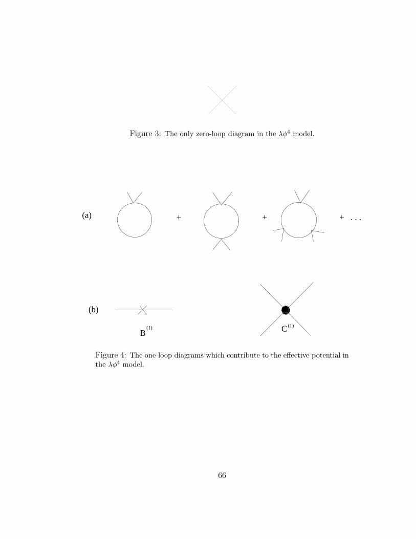
Figure 3: The only zero-loop diagram in the λφ4 model.
������
������
���
���
������
������
+ + + . . .(a)
(b)
B(1) C (1)
Figure 4: The one-loop diagrams which contribute to the effective potential inthe λφ4 model.
66
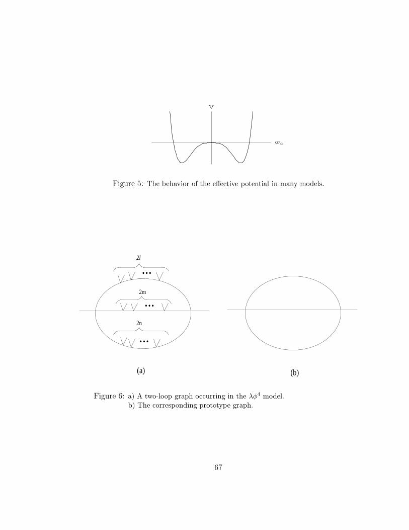
jc
V
Figure 5: The behavior of the effective potential in many models.
2m
2l
2n
...
...
...
(a) (b)
Figure 6: a) A two-loop graph occurring in the λφ4 model.b) The corresponding prototype graph.
67
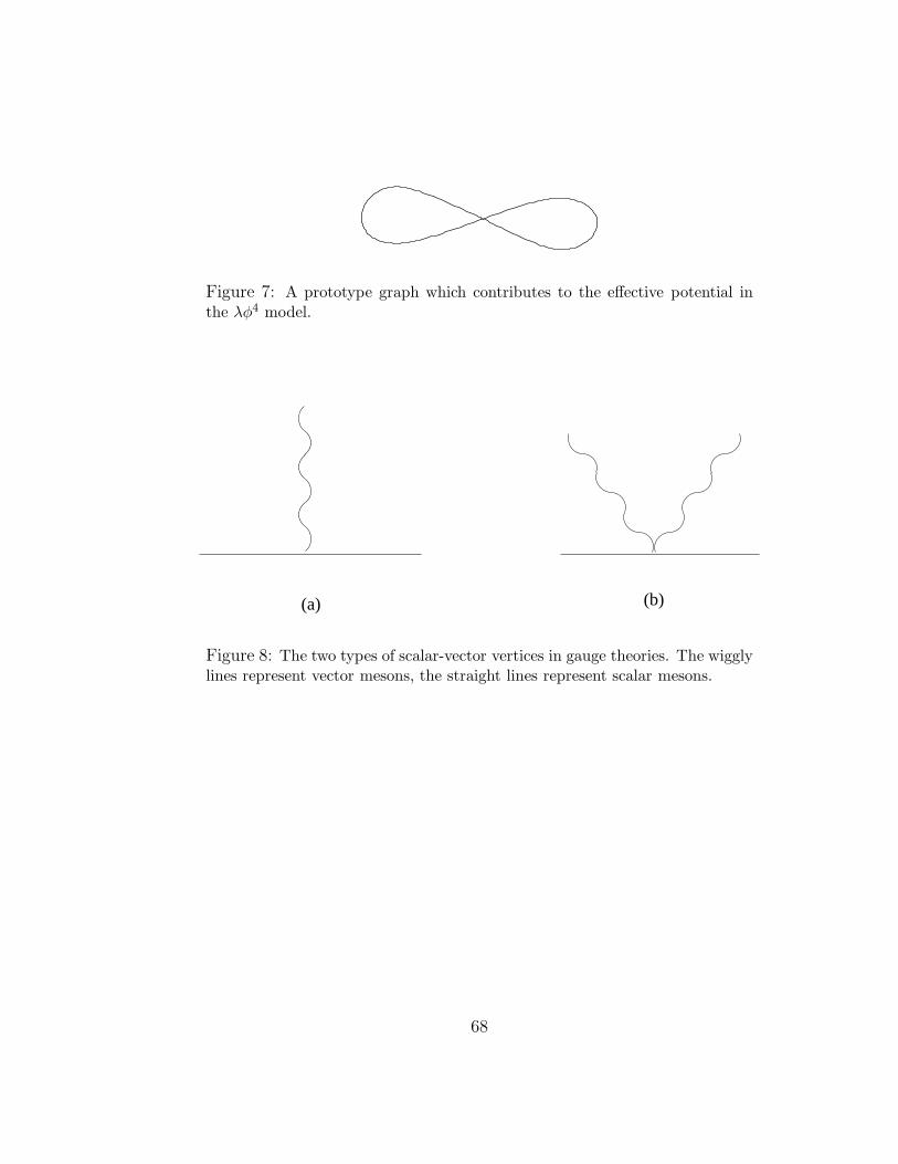
Figure 7: A prototype graph which contributes to the effective potential inthe λφ4 model.
(a) (b)
Figure 8: The two types of scalar-vector vertices in gauge theories. The wigglylines represent vector mesons, the straight lines represent scalar mesons.
68
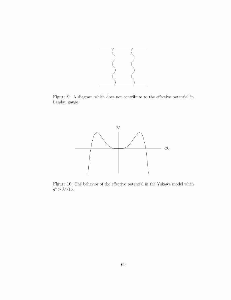
Figure 9: A diagram which does not contribute to the effective potential inLandau gauge.
jc
V
Figure 10: The behavior of the effective potential in the Yukawa model wheng4 > λ2/16.
69
1/e 1x
-1/e
f(x)
Figure 11: The function f(x) = x log(x).
70
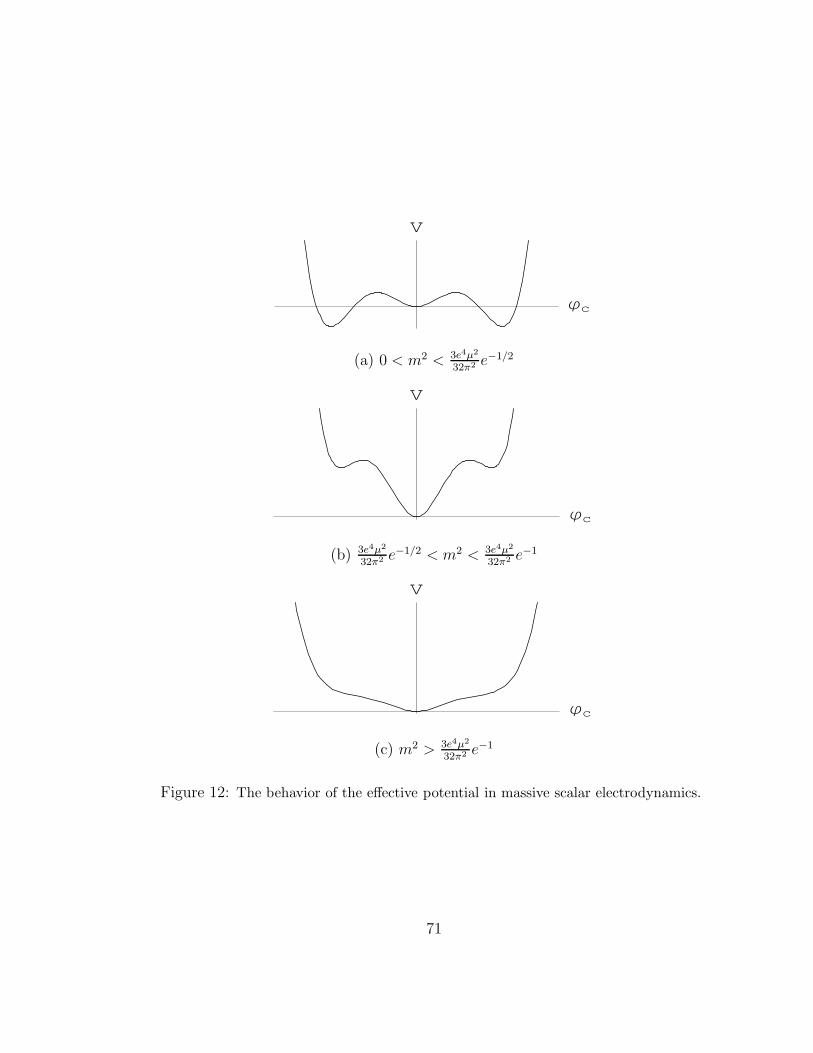
jc
V
(a) 0 < m2 < 3e4µ2
32π2 e−1/2
jc
V
(b) 3e4µ2
32π2 e−1/2 < m2 < 3e4µ2
32π2 e−1
jc
V
(c) m2 > 3e4µ2
32π2 e−1
Figure 12: The behavior of the effective potential in massive scalar electrodynamics.
71
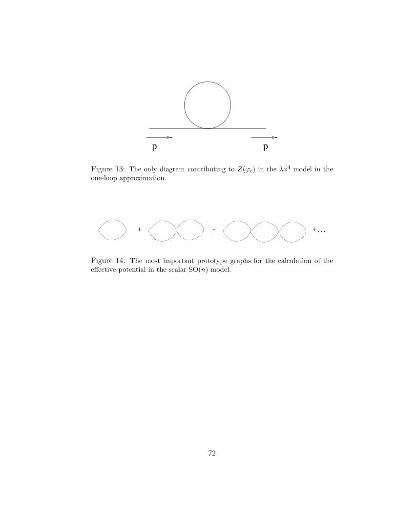
p p
Figure 13: The only diagram contributing to Z(ϕc) in the λφ4 model in theone-loop approximation.
+ + . . .+
Figure 14: The most important prototype graphs for the calculation of theeffective potential in the scalar SO(n) model.
72
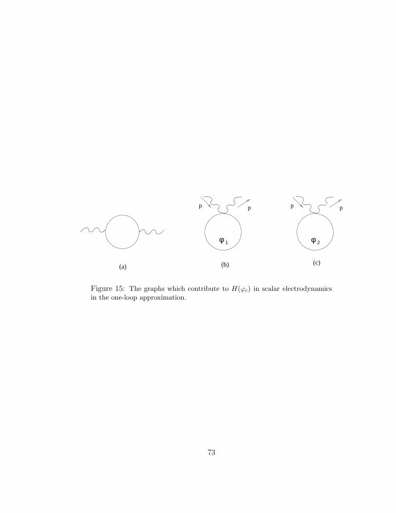
pp
φ
pp
φ 21
(a) (b) (c)
Figure 15: The graphs which contribute to H(ϕc) in scalar electrodynamicsin the one-loop approximation.
73
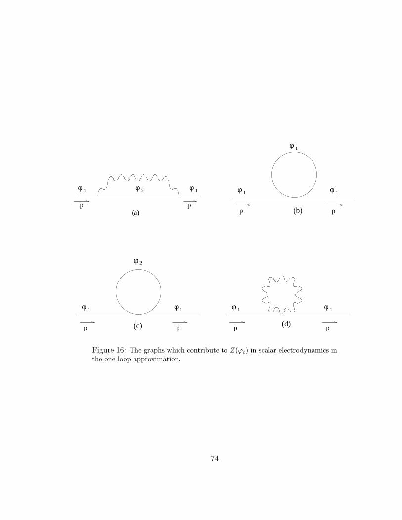
φ 1
p p
φ 1
φ 1
φ 1
p
φ
p
φ2 1
φ2
φ 1
p p
φ 1 φ 1
p p
φ 1
(a) (b)
(c) (d)
Figure 16: The graphs which contribute to Z(ϕc) in scalar electrodynamics inthe one-loop approximation.
74
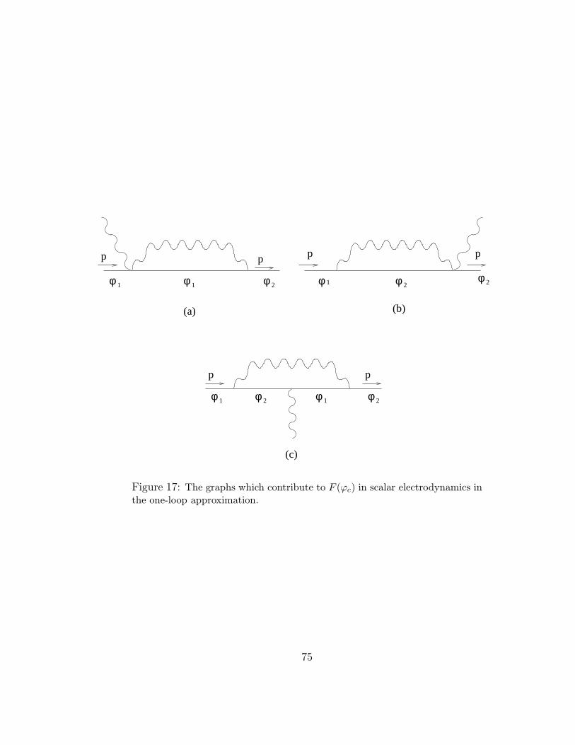
φ φ φ φ
p
1 2 1 2
p
φ 1 φ 2φ φ φ φ
p
1 12 2
p pp
(a) (b)
(c)
Figure 17: The graphs which contribute to F (ϕc) in scalar electrodynamics inthe one-loop approximation.
75
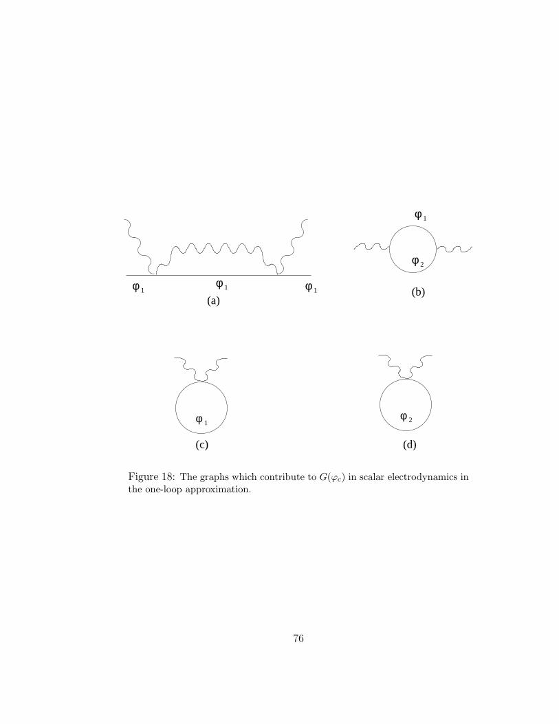
φ φ
φ φ φ
φ
φ
(b)
(c) (d)
(a)1 1
1
2
2
1
1
Figure 18: The graphs which contribute to G(ϕc) in scalar electrodynamics inthe one-loop approximation.
76
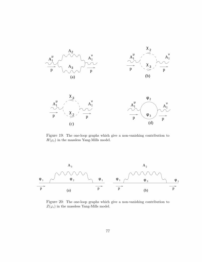
χ3p p
A1µ
A1ν
χ2
p p
A1µ A1
νA2
A3
χ2p p
A1µ
A1ν
χ3
p p
A1µ
A1ν
φ2
φ3
(a) (b)
(c) (d)
Figure 19: The one-loop graphs which give a non-vanishing contribution toH(ϕc) in the massless Yang-Mills model.
AA
(b)(a)
φ φ φ φ φ
p p p p
1 131
3 2
2 φ 1
Figure 20: The one-loop graphs which give a non-vanishing contribution toZ(ϕc) in the massless Yang-Mills model.
77
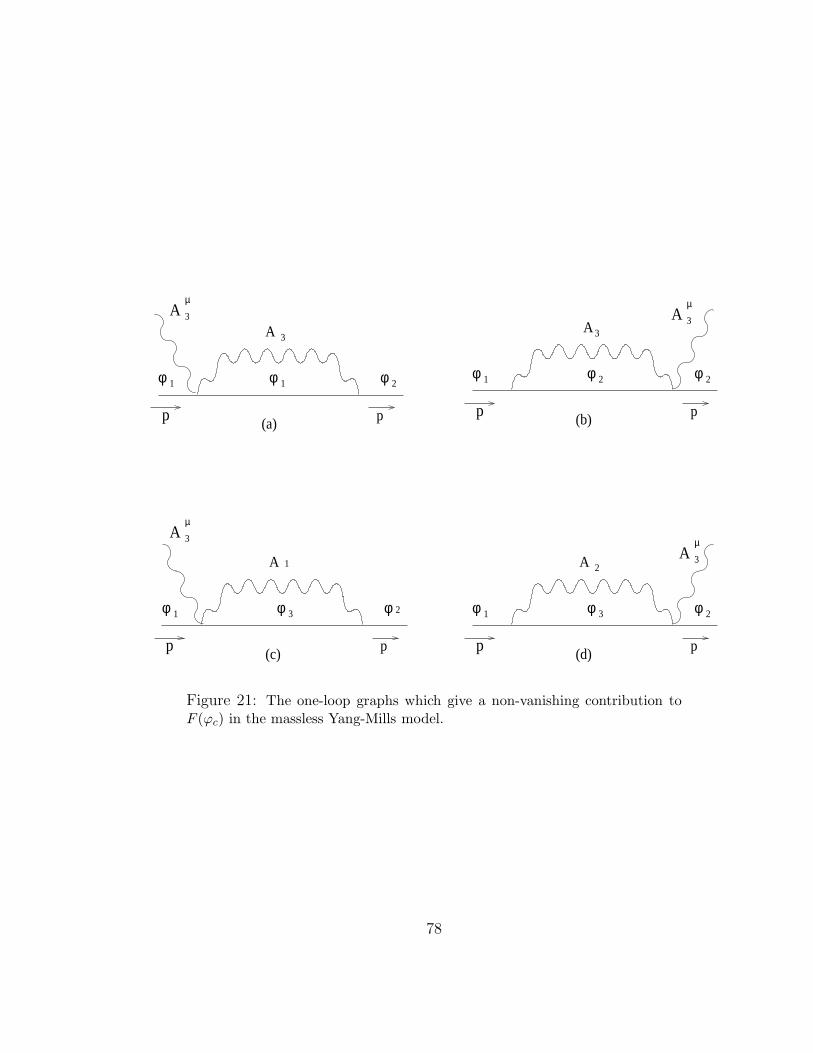
A 3A 3
A 1 A 2
A 3
µ
A 3
µ
A 3
µ
A 3
µ
φ
p
1 φ φ φ
p
1 2 φ
φ φ
p
1 φφ φ
p
1 φ
φ 1
3 3
2 2
22
p
p p
p(a) (b)
(c) (d)
Figure 21: The one-loop graphs which give a non-vanishing contribution toF (ϕc) in the massless Yang-Mills model.
78


![Standard Model: An Introduction - arXiv.org e-Print archive Model: An Introduction ... 3.1 Radiative Corrections to the Standard Model . . . . . . . 64 ... 1971 ⋆ ’t Hooft [73]:](https://static.fdocuments.net/doc/165x107/5afa11df7f8b9abd588dcb1f/standard-model-an-introduction-arxivorg-e-print-archive-model-an-introduction.jpg)