Radiation-induced growth and isothermal decay of infrared-stimulated luminescence from feldspar

Benny Guralnik, Bo Li, Mayank Jain, Reuven Chen, Richard B. Paris, Andrew S. Murray, Sheng-Hua Li, Vasilis Pagonis, Pierre G. Valla, Frédéric Herman

This is the accepted manuscript © 2015, ElsevierLicensed under the Creative Commons Attribution-NonCommercial-NoDerivatives 4.0 International http://creativecommons.org/licenses/by-nc-nd/4.0/

The published article is available from doi:http://dx.doi.org/10.1016/j.radmeas.2015.02.011

1

Radiation-induced growth and isothermal decay of infrared-

stimulated luminescence from feldspar

Benny Guralnik a,*, Bo Li b, Mayank Jain c, Reuven Chen d, Richard B. Paris e,

Andrew S. Murray f, Sheng-Hua Li g, Vasilis Pagonis h, Pierre G. Valla i,

Frédéric Herman i a Department of Earth Sciences, ETH-Zurich, 8092 Zurich, Switzerland

b Centre for Archaeological Science, School of Earth and Environmental Sciences, University of

Wollongong, Wollongong, NSW 2522, Australia.

c Centre for Nuclear Technologies, Technical University of Denmark, DTU Risø campus, DK 4000

Roskilde, Denmark.

d Raymond and Beverly Sackler School of Physics and Astronomy, Tel-Aviv University, 69978 Tel-

Aviv, Israel.

e University of Abertay, Dundee, DD1 1HG, UK.

f Nordic Laboratory for Luminescence Dating, Department of Geoscience, Aarhus University, DTU

Risø Campus, Denmark

g Physics Department, McDaniel College, Westminster, MD 21157, USA.

h Department of Earth Sciences, The University of Hong Kong, Pokfulam Road, Hong Kong, China.

i Institute of Earth Surface Dynamics, University of Lausanne, Geopolis, 1015 Lausanne, Switzerland.

* Corresponding author. Present address: Netherlands Centre for Luminescence Dating,

Droevendaalsesteeg 4, 6708 PB Wageningen, The Netherlands.

E-mail address: benny.guralnik@gmail.com (B. Guralnik)

Abstract

Optically stimulated luminescence (OSL) ages can determine a wide range of

geological events or processes, such as the timing of sediment deposition, the

exposure of a rock surface, or the cooling of bedrock. The accuracy of OSL dating

critically depends on our capability to describe the growth and decay of laboratory-

regenerated luminescence signals. Here we review a selection of common models

describing the response of infrared stimulated luminescence (IRSL) of feldspar to

constant radiation and temperature as administered in the laboratory. We use this

opportunity to introduce a general-order kinetic model that successfully captures the

behaviour of different materials and experimental conditions with a minimum of

model parameters, and thus appears suitable for future application and validation in

natural environments. Finally, we evaluate all the presented models by their ability to

accurately describe a recently published feldspar multi-elevated temperature post-IR

IRSL (MET-pIRIR) dataset, and highlight each model’s strengths and shortfalls.

2

1. Introduction

Optically stimulated luminescence (OSL) dating of feldspar, commonly

utilising stimulation with infrared (IR) light and hence termed IRSL, is a group of

methods enabling the determination of depositional ages of middle to late

Quaternary sediments (Hütt et al., 1988; Buylaert et al., 2012; Li et al., 2014). More

recently, the geological applications of feldspar IRSL have been extended to surface

exposure dating (Sohbati et al., 2011) and low-temperature thermochronology

(Guralnik et al., under review). In addition to the chemical or physical

characterisation of a sample’s natural radioactivity, the conversion of its natural

luminescence into a radiometric age involves two laboratory experiments, in which

the luminescence is monitored as a function of the exposure time t [s] to (i) a source

of constant radioactivity D [Gy s-1], and (ii) a source of a constant temperature T

[K]. The former experiment determines how fast does the luminescence signal grow

under an artificial radiation source, and the latter (often skipped in routine sediment

dating) quantifies the thermal stability of the dosimetric electron trap.

Although the observable rates of luminescence growth and decay in the

laboratory are typically faster by a factor of ~1010 than in nature, geological dating

must assume that the kinetic parameters describing laboratory behaviour are

fundamental physical characteristics of the material, that can be extrapolated over

longer timescales and slower rates. Thus, the selection of a model for describing

laboratory behaviour is more than critical for the correct and meaningful conversion

of the natural luminescence intensities into equivalent ages. Even if a model

produces an excellent fit to laboratory data, this cannot necessarily guarantee its

successful extrapolation to geological timescales; at the same time, a model which

does not fit laboratory data is even harder to evaluate, since it may further propagate

this failure unpredictably, potentially yielding correct ages even though the model is

inadequate. In this paper, we take a fresh look at the conventional ‘status quo’

models currently used to describe dose response and thermal sensitivity of feldspar

IRSL. We further examine an interesting heuristic approach (the General-Order

Kinetic model), and use a representative dataset to graphically illustrate the key

differences between the models, and to quantify their relative successes and

shortfalls.

3

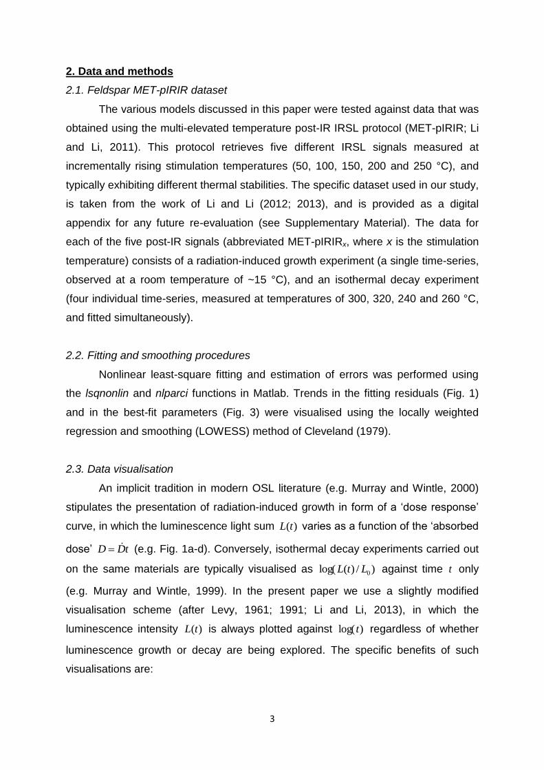
2. Data and methods

2.1. Feldspar MET-pIRIR dataset

The various models discussed in this paper were tested against data that was

obtained using the multi-elevated temperature post-IR IRSL protocol (MET-pIRIR; Li

and Li, 2011). This protocol retrieves five different IRSL signals measured at

incrementally rising stimulation temperatures (50, 100, 150, 200 and 250 °C), and

typically exhibiting different thermal stabilities. The specific dataset used in our study,

is taken from the work of Li and Li (2012; 2013), and is provided as a digital

appendix for any future re-evaluation (see Supplementary Material). The data for

each of the five post-IR signals (abbreviated MET-pIRIRx, where x is the stimulation

temperature) consists of a radiation-induced growth experiment (a single time-series,

observed at a room temperature of ~15 °C), and an isothermal decay experiment

(four individual time-series, measured at temperatures of 300, 320, 240 and 260 °C,

and fitted simultaneously).

2.2. Fitting and smoothing procedures

Nonlinear least-square fitting and estimation of errors was performed using

the lsqnonlin and nlparci functions in Matlab. Trends in the fitting residuals (Fig. 1)

and in the best-fit parameters (Fig. 3) were visualised using the locally weighted

regression and smoothing (LOWESS) method of Cleveland (1979).

2.3. Data visualisation

An implicit tradition in modern OSL literature (e.g. Murray and Wintle, 2000)

stipulates the presentation of radiation-induced growth in form of a ‘dose response’

curve, in which the luminescence light sum )(tL varies as a function of the ‘absorbed

dose’ tDD (e.g. Fig. 1a-d). Conversely, isothermal decay experiments carried out

on the same materials are typically visualised as )/)(log( 0LtL against time t only

(e.g. Murray and Wintle, 1999). In the present paper we use a slightly modified

visualisation scheme (after Levy, 1961; 1991; Li and Li, 2013), in which the

luminescence intensity )(tL is always plotted against )log(t regardless of whether

luminescence growth or decay are being explored. The specific benefits of such

visualisations are:

4

(i) Separation of data from interpretation. When luminescence )(tL is plotted

against the absorbed dose tDD , the x-axis unnecessary entangles a primary

observation (irradiation time t ) with a derived parameter (the dose rate D ), the

latter incorporating multiple internal and external uncertainties (Bos et al., 2006;

Guerin et al., 2012; Kadereit and Kreutzer, 2013; Boehnke and Harrison, 2014).

Thus, a plot of )(tL vs. D technically becomes erroneous with every systematic

revision of dose rate conversion factors, while a plot of )(tL vs. t will not only

remain valid, but also be easier to re-analyse in the future. Furthermore, it is

well-known that in materials suffering from athermal losses, delivery of the same

dose at different irradiation rates leads to differential luminescence responses

(e.g. Kars et al., 2008). Thus, showing luminescence response against an

amalgamated variable which is the product of both time and dose rate tDD

leads to misapprehension of the dependence of luminescence build-up on

laboratory dose rates (see Levy, 1961; 1991).

(ii) Visual informativeness: The processes of luminescence growth and decay are

both governed by a fundamental rate term [s-1], which drives each corresponding

process towards a secular steady-state. Derivation of reliable kinetic parameters

typically relies on data which is uniformly spaced across 3-4 orders of magnitude

of time (e.g. Kars et al., 2008; Murray et al., 2009; Timar-Gabor et al., 2012).

Thus, the use of a linear time axis may unfavourably compress information from

a particular timescale, and lead to a visual misapprehension on fit quality, or the

lack of experimental points to (dis)prove a certain model (compare Fig 1a-d with

Fig. 1e-h, showing exactly the same data )(tL but as a function of tDD and

)log( t , respectively). The above problems are less likely to occur on a

logarithmic time axis )log(t , which not only grants easy comparison between

similar processes occurring on different timescales, but also highlights regions

where data is missing to properly constrain the model fitting

(iii) Uniformity for internal comparison: Visualisation of luminescence growth and

decay as a function of )log(t allows a straightforward side-by-side comparison of

the kinetic responses of the material to cumulative irradiation and heat, and

facilitates both the detection and quantification of systematic departure from first

order kinetics in both cases (see Section 3.3 and Fig. 2). Although the new

5

standardised visualisation might be slightly difficult to compare to former studies

(utilising the more familiar visualisations), we believe that this is a minor

inconvenience outweighed by the benefits of internal intercomparison, and of an

enhanced apprehension of model quality.

[Figure 1]

3. Models and results

3.1. First-order (exponential) kinetics (1EXP)

The growth of the IRSL light sum )(tL [a.u.] in a feldspar exposed to a

radioactive source may be described by a saturating exponential function:

)/exp(1/)( 0max DtDLtL (1)

(e.g. Balescu et al., 1997; Li and Li, 2012) where maxL [a.u.] is the maximum

luminescence light sum, D [Gy s-1] the constant dose rate of the radioactive source,

t [s] the time, and 0D [Gy] the characteristic dose. Similarly, the time-evolution of

)(tL [a.u.] under isothermal storage of the feldspar at temperature T [K] may be

described by a decaying exponential function:

tseLtLTkE B

/

0 exp/)( (2)

(e.g. Li et al., 1997; Murray et al., 2009), where 0L [a.u.] is the initial IRSL light sum,

E [eV] and s [s-1] the Arrhenius parameters (activation energy and the attempt-to-

escape frequency, respectively), Bk [eV K-1] Boltzmann’s constant, and t [s] the

time as before.

Figures 1a,e and 1i demonstrate the rather unsatisfactory fits of the 1EXP

model to the irradiation response (top plots in Figs. 1a,e) and isothermal decay (Fig.

1i) of the MET-pIRIR250 signal. Although for luminescence growth (top plots in Figs.

1a,e), the 1EXP model explains ~99% of the variance in the data, the residuals are

not normally distributed over the time domain (bottom plot in Figs. 1a,e), stipulating

the search for a better model. For the isothermal decay data, the overall R2 of 1EXP

(~85% in Fig. 1i) is grossly overestimating the individual R2 for each holding

temperature, and thus evaluates this model as inappropriate.

6

3.2. Multi-exponential kinetics (mEXP)

Observation of slow but steady growth of feldspar IRSL at high doses

( 0DtD ) is often empirically explained by a saturating exponential plus linear

(1EXP+LIN) model:

0201 /)/exp(1)( DtDLDtDLtL (3)

(e.g. Lai, 2010), where 1L and 2L [a.u.] are the saturating exponential and linear

components, respectively (typically 12 LL ). Although such linear growth may be

interpreted as a steady generation of new electron traps at a fixed rate (e.g. Levy,

1961), this phenomenon is more often viewed as the early expression of a second

saturating exponential, corresponding to a different component or sub-population of

the electron trap (Chen et al., 2001). Following the reasoning of signal break-up into

individual components, the dose response of feldspar IRSL may be generalized to:

m

ii DtDLtL1

,0 )/exp(1)( (4)

where m=2 usually suffices (e.g. Thomsen et al., 2011; Buylaert et al., 2012), and

where iL [a.u.] and iD ,0 [Gy] are the maximum light sum and characteristic dose of

the i -th component. To justify the 2EXP model in quartz OSL, several working

hypotheses have been put forth (Lowick et al., 2010; Berger and Chen, 2011; Timar-

Gabor et al., 2012), but the phenomenon is still poorly understood (Wintle, 2011).

From the chemical standpoint, the possibility of distinct dose-response components

in feldspar is even more likely than in quartz (e.g. different 0D values for each

compositional end-member of feldspar; cf. Barré and Lamothe, 2010), however this

conjecture is pending further proof.

Fits of 1EXP+LIN and 2EXP to the MET-pIRIR250 dataset are shown in Figs.

1b-c and 1f-g. From inspecting the residuals, it may be seen that 2EXP performs

better due to one extra model parameter. However, the dataset is in fact insufficient

to justify the break-up into the best-fit dose components 1,0D =122±30 Gy and

2,0D =490±60 Gy, as the 0D values are too closely spaced (see review by Istratov

and Vyvenko, 1999). Interestingly, neither of the above values, nor the 0D =244±9 Gy

from 1EXP+LIN, overlap with the baseline value of 0D =315±8 Gy, retrieved by not

necessarily the correct, yet the simplest 1EXP model.

7

Switching to multi-exponential description of isothermal loss, we start with the

model of Jain et al. (2012), who expressed the thermal loss of trapped charges via a

quantum mechanical tunnelling from the excited state of the electron trap. In the

resulting multi-exponential system (where first-order loss occurs only for a fixed

electron-hole separation distance), the decrease of luminescence intensity with

progressive isothermal storage can be approximated by:

3/

0 8.11lnexp/)( tseLtLTkE B

(5)

(Kitis and Pagonis, 2013), where 0L [a.u.] is the initial intensity, and the scaled

density of the nearest-neighbour distribution of holes. Notably, Eq. (5) reduces to the

athermal tunnelling model of Huntley (2006) upon the substitution 0E , thereby

generalising Huntley’s model to thermally-assisted processes. The fit of Eq. (5) to the

MET-pIRIR250 data is shown in Fig. 1i, with narrowly constrained parameters and no

appreciable time dependence or structure in the residuals.

A different multi-exponential approach was taken by Li and Li (2013), who

assumed that trapped electrons are thermally activated to discrete and exponentially

distributed energy levels below the conduction band (known as band tail states,

Poolton et al., 2002; 2009). Envisaging a spatial distribution where each electron trap

is associated with only one band-tail energy level above it, Li and Li (2013)

expressed the overall thermal decay of luminescence as:

b

E

tseEEdEeeLtL

TBkbEEub

0

/

0

/)(

/)( (6a)

where 0L [a.u.] is the initial intensity, and uE [eV] is the Urbach band-tail width. Eq.

(6a) reduces to Eq. (2) for 0bE , and thereby qualifies as its logical extension. To

derive a convenient approximation for Eq. (6a) for data fitting, we introduce

TkEb Bb / , TkEu Bu / , and TkE Bset/

, and rewrite Eq. (6a) as:

dueeTkLtL

b

eub

B

b

0

0

/

0/)( (6b)

To bypass tedious numerical integration, this paragraph derives a convenient

analytical approximation for Eq. (6b), which can be easily implemented in common

curve-fitting software. We begin by a change of variables bew and rearrange the

latter into wdwdbwb /,ln , to obtain:

8

),/1(),/1(/)( 0

00

/1/11/1

1

/11

0

bu

B

w

xuu

B

w

wu

B euuTkdxexTkdwewTkLtL

(6c)

where is the upper incomplete gamma function. Back-substitution of the original

variables, and omission of the negligible second term results in:

TkE

uB

ETkTkE

BB

uBB setETksetTkLtL

///

0 ,//)(

(6d)

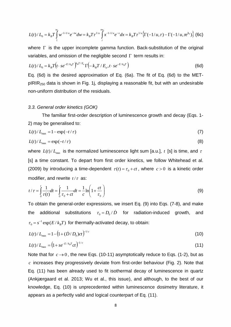
Eq. (6d) is the desired approximation of Eq. (6a). The fit of Eq. (6d) to the MET-

pIRIR250 data is shown in Fig. 1j, displaying a reasonable fit, but with an undesirable

non-uniform distribution of the residuals.

3.3. General order kinetics (GOK)

The familiar first-order description of luminescence growth and decay (Eqs. 1-

2) may be generalised to:

)/exp(1/)( max tLtL (7)

)/exp(/)( max tLtL (8)

where max/)( LtL is the normalized luminescence light sum [a.u.], t [s] is time, and

[s] a time constant. To depart from first order kinetics, we follow Whitehead et al.

(2009) by introducing a time-dependent ctt 0)( , where 0c is a kinetic order

modifier, and rewrite /t as:

00 00

1ln11

)(

1/

ct

cdt

ctdt

tt

tt

(9)

To obtain the general-order expressions, we insert Eq. (9) into Eqs. (7-8), and make

the additional substitutions DD /00 for radiation-induced growth, and

)/exp(1

0 TkEs B

for thermally-activated decay, to obtain:

cctDDLtL

/1

0max )/(11/)(

(10)

cTkEctseLtL B

/1/

max 1/)(

(11)

Note that for 0c , the new Eqs. (10-11) asymptotically reduce to Eqs. (1-2), but as

c increases they progressively deviate from first-order behaviour (Fig. 2). Note that

Eq. (11) has been already used to fit isothermal decay of luminescence in quartz

(Ankjærgaard et al. 2013; Wu et al., this issue), and although, to the best of our

knowledge, Eq. (10) is unprecedented within luminescence dosimetry literature, it

appears as a perfectly valid and logical counterpart of Eq. (11).

9

[Figure 2]

To further explore the placement of Eqs. (10-11) within the context of general-

order kinetics, we differentiate both equations with respect to time, assume the

standard proportionality between luminescence and trapped charge ( ntL )( ,

NL max ), and make a convenient variable replacement ( 1 c , 1 c ) to

translate Eqs. (10-11) into:

N

n

D

D

N

n

dt

d1

0

(12)

N

nse

N

n

dt

d TkE B/ (13)

in which n is the number of electrons trapped in N traps of a certain type [both a.u.],

and and are the kinetic orders [a.u.] of the electron trapping and detrapping

reactions, respectively.

The effect of the unitless kinetic orders and on the luminescence growth

and decay is graphically shown in Fig. 2 and discussed below. In first-order kinetics

)1,1( the growth and decay rates of luminescence are always independent of

the amount of trapped charge Nn / (thus justifying the definition of a trap lifetime).

Conversely, in higher order kinetics )1,1( reaction do depend on trap

occupation, and always progress at slower-than-exponential rates. This may be

mathematically appreciated by looking at Eqs. 12-13, where the fractions of empty

and filled electron traps ( Nn /1 and Nn / , respectively), always smaller than unity,

are both further diminished when raised to a power of 1,1 .

From the physical standpoint, the progressive slowdown of reaction rates in

systems which are nearly empty or borderline their full capacity (i.e. close to the

boundary conditions) is both understandable and predictable. Specifically, the

slower-than-exponential electron detrapping ( 1 ) has been often considered in the

luminescence literature (e.g. Wise, 1951; May and Partridge, 1964; Rasheedy,

1993), and explained in terms of electron retrapping or distance-dependent

probabilities. Conversely, the slower-than-exponential trapping of electrons ( 1 ) in

a confined volume due to the gradual build-up of Coulomb repulsive forces is a well-

studied phenomenon in field-effect transistors (e.g. Sune et al., 1990; Williams,

10

1992). Buildup of Coulomb forces, and the presently overlooked effects of possible

charge disequilibrium within irradiated crystals, are both subjects of increasing

interest within the luminescence dating community, stipulating new research

directions being currently underway (J.-P. Buylaert, pers. comm.).

While a further physical validation of Eqs. (12-13) remains outside of the

scope of the present work, we note that their superposition results in:

N

nse

N

n

D

D

N

n

dt

d TkE B/

0

1

(15)

which for 1 reduces to the familiar description of thermoluminescence

systems (Christodoulides et al., 1971), and for 1, serves as its logical extension

for more complex (i.e. slowed-down) behaviour.

The fits of Eqs. (10-11) to the MET-pIRIR250 growth and decay are shown in

Figs. 1d,h and 1k, respectively. Interestingly, the 0D ’s recovered by the 1EXP and

GOK models are indistinguishable; from this perspective, GOK is the only extended

model which introduces a further complexity without affecting the primary response

variable ( 0D ) as obtained from the least sophisticated model (Eq. 1). For the

isothermal holding, the GOK model fits the experimental dataset equally well as

mEXP tunnelling, further exhibiting the narrowest confidence intervals.

4. Discussion

The best-fit kinetic parameters for the MET-pIRIR250 signal from Fig. 1 are

summarised in Fig. 3 (filled circles) and further supplemented by the best-fit

parameters from the other four MET-pIRIR signals (MET-pIRIR50 – MET-pIRIR200).

Starting with the radiation-induced growth dataset (Fig. 3a-d), it seems that

irrespective of the chosen model, 0D appears to be anti-correlated with the MET

stimulation temperature, yielding progressively smaller 0D ’s for the least fading

signals (pIR200 and pIR250). Although compared to 1EXP, the multicomponent

1EXP+LIN and the 2EXP models appear as plausible fits on the typical ‘dose-

response’ curves (Figs. 1b-c), they appear as unconstrained over-fitting artefacts,

lacking model verification in their high-dose domain (clearly seen as the

unconstrained model predictions in Figs. 1f-g), and therefore raising further concern

for their use for predicting minimum ages or thermal closure ages, where the steady-

11

state response of the system becomes a crucial consideration. The GOK model

looks promising not only because it fits the experimental data best with a minimum of

model parameters, but also because it retains the same 0D ’s as the simplest 1EXP

model; however, the validity of this approach both in the high-dose region and within

natural environments, is clearly subject to further investigation.

For the isothermal decay dataset (Figs. 3e-h), the 1EXP model seems

absolutely inadequate. In the bandtail mEXP, tunnelling mEXP and GOK models,

there is a clear correlation between a single response variable ( uE , 10log or c )

with the post-IR stimulation temperature, which the Arrhenius parameters assuming

E and s remain semi-constant. However, a high covariance between E and uE in

the bandtail mEXP points to an ill-conditioned fit, to be addressed though a

reduction of the number of parameters (e.g. assuming E , uE or s to be constant; cf.

Li and Li, 2013). The tunnelling mEXP model yields kinetic parameters that are

supported in literature, including a familiar s value in the range 1012 – 1014 s-1, and

E ~1.4 eV corresponding to the optical energy of the excited state; how these results

apply to pIRIR signals involving transitions through band tail states is a separate

question worth investigating (see Jain et al., this volume). The GOK model yields

E ~1.3 eV and s ~109, both of which are anomalously low compared to familiar

literature values (Li et al., 1997; Murray et al., 2009; Li and Li, 2013). While the

extrapolation of these kinetic parameters to geological timescales seems to be

successful (Guralnik et al., subm.), additional effort is required to understand

whether these best-fit parameters fold in the initial experimental conditions of the

explored systems (cf. Rasheedy, 1993).

[Figure 3]

Although heuristic, the proposed GOK model offers a convenient and self-

consistent alternative to the more established multi-exponential analysis, yielding

plausible fits to experimental data with a comparable (or fewer) number of model

parameters, and a well-known physical reasoning. Although the dataset is too small

to allow a meaningful statistical inference (n=5), it is worthwhile to note that the

kinetic orders of dose response (Fig. 3d) and isothermal holding (Fig. 3h) appear to

be pairwise correlated. This suggests that a particular system’s departure from first-

12

order kinetics (Fig. 2) may be manifested in mirroring electron trapping and

detrapping processes. This observation further justifies the proposed uniform

visualisation )(tL vs. )log(t for both dose response and isothermal holding

experiments, as it may help identify and correlate the departure from first-order

kinetics in both these processes. Furthermore, the hypothesized correlation

invites to consider a continuous multi-exponential fitting (Eqs. 5 or 6) for the

description of dose response in feldspar, which is currently only modelled by a finite

and usually small number of dose-response components.

The present study has focused on evaluating the different feldspar models

against a set of laboratory experiments, where the rates of electron trapping and

detrapping are roughly ~1010 times faster than in typical natural settings. The next

desirable step would be to test these models in natural conditions, where there is a

maximum number of independent constraints on the sedimentation age, the duration

of surface exposure, or the thermal regime. Noticeable mismatches between

laboratory and natural dose response curves (Chapot et al., 2012; Zander and

Hilgers, 2013) stipulate the evaluation of all models in their high-dose (steady-state)

region, not regularly covered by standard laboratory measurements (Fig. 1e-h).

Better characterisation of the high-dose region would also be beneficial for minimum

age reporting (e.g. Joordens et al., 2014) or for thermochronological interpretation

(Guralnik et al., 2013). In particular, the applicability of the general-order kinetics

(GOK) model to natural conditions seems very promising, and will be reported

elsewhere (Wu et al., this volume; Ankjærgaard et al., this volume; Guralnik et al.,

under review).

5. Conclusions

This paper reviewed common models describing dose response and

isothermal decay in feldspar IRSL dating, and introduced a self-consistent general

order kinetic model which produces good fits to laboratory data. As a first step

towards proper model evaluation and intercomparison, we promote the use of a

logarithmic time axis for the visualisation of both dose response and isothermal

holding experiments. As a second step, we have demonstrated that representative

feldspar IRSL data cannot be adequately described by first-order kinetics, while

some of the common multi-exponential approaches are seen to suffer from

13

covariated (and thus potentially non-identifiable) parameters. The proposed general

order kinetics model captures both the laboratory dose response and isothermal

decay of feldspar IRSL well, but may only be a gross mathematical simplification of

actual physical processes; nevertheless it is a promising path towards

methodological standardisation, stipulating further basic research and comparative

model verification in well-constrained geological environments.

7. Acknowledgements

This work was supported by the Swiss National Foundation grants 200021-

127127 (FH and BG) and PZ00P2-148191 (PGV), and has benefitted from

stimulating discussions with David Sanderson, Christina Ankjærgaard and Sally

Lowick.

8. References Ankjærgaard, C., Jain, M., Wallinga, J., 2013. Towards dating Quaternary sediments using the quartz Violet

Stimulated Luminescence (VSL) signal. Quat. Geochron. 18, 99–109.

Ankjærgaard, C., Guralnik, B., Porat, N., Heimann, A., Jain, M., Wallinga, J., (this volume). Violet stimulated

luminescence: geo- or thermochronometer? Radiat. Meas.

Balescu, S., Lamothe, M., Lautridou, J.P., 1997. Luminescence evidence for two Middle Pleistocene interglacial

events at Tourville, northwestern France. Boreas, 26, 61-72.

Barré, M., Lamothe, M., 2010. Luminescence dating of archaeosediments: a comparison of K-feldspar and

plagioclase IRSL ages. Quat. Geochron. 5, 324-328.

Berger, G.W., 1990. Regression and error analysis for a saturating-exponential-plus-linear model. Ancient TL,

8, 23-25.

Berger, G.W., Chen, R., 2011. Error analysis and modelling of double saturating exponential dose response

curves from SAR OSL dating. Ancient TL 29, 9–14.

Boehnke, P., Harrison, T. M., 2014. A meta-analysis of geochronologically relevant half-lives: what’s the best

decay constant? Int. Geol. Rev. 56, 905-914.

Bos, A.J.J., Wallinga, J., Johns, C., Abellon, R.D., Brouwer, J.C., Schaart, D.R., Murray, A.S., 2006. Accurate

calibration of a laboratory beta particle dose rate for dating purposes. Radiat. Meas. 41, 1020-1025.

Buylaert, J.P., Jain, M., Murray, A.S., Thomsen, K.J., Thiel, C., Sohbati, R., 2012. A robust feldspar

luminescence dating method for Middle and Late Pleistocene sediments. Boreas 41, 435-451.

Chapot, M.S., Roberts, H.M., Duller, G.A.T., Lai, Z.P., 2012. A comparison of natural-and laboratory-generated

dose response curves for quartz optically stimulated luminescence signals from Chinese Loess. Radiat.

Meas. 47, 1045-1052.

Chen, G., Murray, A.S., Li, S.H., 2001. Effect of heating on the quartz dose-response curve. Radiat. Meas. 33,

59-63.

Christodoulides, C., Ettinger, K.V., Fremlin, J.H., 1971. The use of TL glow peaks at equilibrium in the

examination of the thermal and radiation history of materials. Modern Geology 2, 275–280.

Cleveland, W.S., 1979. Robust locally weighted regression and smoothing scatterplots. J. Am. Stat. Assoc. 74,

829-836.

Guérin, G., Mercier, N., Adamiec, G., 2011. Dose-rate conversion factors: update. Ancient TL, 29, 5-8.

Guibert, P., Vartanian, E., Bechtel, F., Schvoerer, M., 1996. Non-linear approach of TL response to dose:

polynomial approximation. Ancient TL, 14, 7-14.

Guralnik, B., Jain, M., Herman, F., Murray, A.S., Valla, P.G., Ankjærgaard, C., Lowick, S.E., Preusser, F.,

Chen, R., Kook, M.H., Rhodes, E.J. (subm.). OSL-thermochronology of bedrock feldspar reveals sub-

Quaternary thermal histories of near- surface rocks.

Guralnik, B., Jain, M., Herman, F., Paris, R.B., Harrison, T.M., Murray, A.S., Valla, P.V., Rhodes, E.J., 2013.

Effective closure temperature in leaky and/or saturating thermochronometers. Earth Planet. Sci. Lett. 384,

209–218.

14

Huntley, D.J., 2006. An explanation of the power-law decay of luminescence. J. Phys. Cond. Matt. 18, 1359–

1365.

Hütt, G., Jaek, I., Tchonka, J., 1988. Optical dating: K-feldspars optical response stimulation spectra. Quat. Sci.

Rev. 7, 381–385.

Istratov, A.A., Vyvenko, O.F., 1999. Exponential analysis in physical phenomena. Rev. Sci. Inst. 70, 1233-

1257.

Jain, M., Guralnik, B., Andersen, M.T., 2012. Stimulated luminescence emission arising from localized

recombination within randomly distributed defects. J. Phys. Cond. Mat., in press.

Joordens, J.C., d’Errico, F., Wesselingh, F. P., Munro, S., de Vos, J., Wallinga, J., Ankjærgaard, C., Reimann,

T., Wijbrans, J.R., Kuiper, K.F., Mücher, H.J., Coqueugniot, H., Prié, V., Joosten, I., van Os, B., Schulp,

A.S., Panuel, M., van der Haas, V., Lustenhouwer, W., Reijmer J.J.G., Roebroeks, W., 2014. Homo erectus

at Trinil on Java used shells for tool production and engraving. Nature, doi:10.1038/nature13962

Kadereit, A., Kreutzer, S., 2013. Risø calibration quartz–A challenge for β-source calibration. An applied study

with relevance for luminescence dating. Measurement 46, 2238-2250.

Kars, R.H., Wallinga, J., Cohen, K.M., 2008. A new approach towards anomalous fading correction for feldspar

IRSL dating—tests on samples in field saturation. Radiat. Meas. 43, 786–790.

Kitis, G., Pagonis, V., 2013. Analytical solutions for stimulated luminescence emission from tunneling

recombination in random distributions of defects. J. Lumin. 137, 109–115.

Lai, Z. P., Stokes, S., Bailey, R., Fattahi, M., Arnold, L., 2003. Infrared stimulated red luminescence from

Chinese loess: basic observations. Quat. Sci. Rev. 22, 961–966.

Levy, P.W., 1961. Color centers and radiation-induced defects in Al2O3. Phys. Rev. 12, 1226-1233.

Levy, P.W., 1991. Radiation damage studies on non-metals utilizing measurements made during irradiation. J.

Phys. Chem. Solids 52, 319–349.

Li, B., Jacobs, Z., Roberts, R.G., Li, S.H., 2014. Review and assessment of the potential of post-IR IRSL dating

methods to circumvent the problem of anomalous fading in feldspar luminescence. Geochronometria, 1-24.

Li, B., Li, S.H., 2008. Investigations of the dose-dependent anomalous fading rate of feldspar from sediments. J.

Phys. D. Appl. Phys. 41, 225502.

Li, B., Li, S.-H., 2011. Luminescence dating of K-feldspar from sediments: A protocol without anomalous

fading correction. Quat. Geochron. 6, 468–479.

Li, B., Li, S.H., 2012. Luminescence dating of Chinese loess beyond 130 ka using the non-fading signal from K-

feldspar. Quat. Geochron. 10, 24–31.

Li, B., Li, S.H., 2013. The effect of band-tail states on the thermal stability of the infrared stimulated

luminescence from K-feldspar. J. Lumin., 136, 5–10.

Li, S.H., Tso, M.Y.W., Wong, N.W., 1997. Parameters of OSL traps determined with various linear heating

rates. Radiat. Meas. 27, 43-47.

Lowick, S.E., Preusser, F., Wintle, A.G., 2010. Investigating quartz optically stimulated luminescence dose–

response curves at high doses. Radiat. Meas. 45, 975–984.

McKeever, S.W.S., Chen, R., 1997. Luminescence models. Radiat. Meas. 27, 625-661.

Murray, A.S., Buylaert, J.P., Thomsen, K.J., Jain, M., 2009. The effect of preheating on the IRSL signal from

feldspar. Radiat. Meas. 44, 554–559.

Murray, A.S., Wintle, A.G., 1999. Isothermal decay of optically stimulated luminescence in quartz. Radiat.

Meas. 30, 119–125.

Murray, A.S., Wintle, A.G., 2000. Luminescence dating of quartz using an improved single-aliquot

regenerative-dose protocol. Radiat. Meas. 32, 57–73.

Poolton, N.R.J., Kars, R.H., Wallinga, J., Bos, A.J.J., 2009. Direct evidence for the participation of band-tails

and excited-state tunnelling in the luminescence of irradiated feldspars. J. Physics Cond. Matt. 21, 485–505.

Sohbati, R., Murray, A.S., Jain, M., Buylaert, J.-P., Thomsen, K.J., 2011. Investigating the resetting of OSL

signals in rock surfaces. Geochronometria 38, 249–258.

Rasheedy, M.S., 1993. On the general-order kinetics of the thermoluminescence glow peak. J. Phys. Cond. Matt.

5, 633–636.

Sune, C.T., Reisman, A., Williams, C.K., 1990. A new electron-trapping model for the gate insulator of

insulated gate field-effect transistors. J. Electron. Mat. 19, 651–655.

Thomsen, K.J., Murray, A.S., Jain, M., 2011. Stability of IRSL signals from sedimentary K-feldspar samples.

Geochronometria, 38, 1–13.

Timar-Gabor, A., Vasiliniuc, Ş., Vandenberghe, D.A.G., Cosma, C., Wintle, A.G., 2012. Investigations into the

reliability of SAR-OSL equivalent doses obtained for quartz samples displaying dose response curves with

more than one component. Radiat. Meas. 47, 740-745.

Whitehead, L., Whitehead, R., Valeur, B., Berberan-Santos, M., 2009. A simple function for the description of

near-exponential decays: the stretched or compressed hyperbola. Am. J. Phys. 77, 173-179.

Williams, C.K., 1992. Kinetics of trapping, detrapping, and trap generation. J. Electron. Mat. 21, 711–720.

15

Wintle, 2010. Future directions of luminescence dating of quartz. Geochronometria 37, 1–7.

Wu, T.-S., Jain, M., Guralnik, B., Murray, A.S., Chen, Y.-G. (subm. to LED2014 proceedings). Evaluation of

Quartz OSL as a thermochronometer for unraveling recent cooling rates in the Hsuehshan Range (Central

Taiwan).

Zander, A., Hilgers, A., 2013. Potential and limits of OSL, TT-OSL, IRSL and pIRIR 290 dating methods

applied on a Middle Pleistocene sediment record of Lake El'gygytgyn, Russia. Clim. Past 9, 719-733.

Figure captions

Figure 1: Irradiation-response (a-h) and isothermal decay (i-l) of feldspar MET-

pIRIR250 signal (filled circles on top panels) as best-fitted by the various models

discussed in the text (lines with 95% confidence interval on top panels), with quoted

best-fit parameters and goodness-of-fit. Fitting residuals and their trends (dots and

lines on the bottom panels) were obtained by LOWESS (locally-weighted scatterplot

smoothing; Cleveland, 1979).

Figure 2: Radiation induced growth (a) and isothermal decay (b) for different kinetic

orders in the range 1-5, obtained via Eqs. (10) and (11) upon the substitutions

1c and 1 c , respectively.

Figure 3: Cross-model summary of the best-fitting parameters for the MET-pIRIR250

signal from Fig. 1 (filled circles), alongside best-fitting parameters for the four lower

temperature MET-pIRIR signals, given as Supplementary Data (hollow circles).

Isothermal holding time (s)

Irradiation time (s)

Dose (kGy)

Lu

min

esce

nce

(L

/L0)

Re

sid

ua

ls

i) k)j) l)

Radiation-induced growth

Isothermal decay

0 0.5 1.51.0 0 0.5 1.51.0 0 0.5 1.51.0 0 0.5 1.51.0

E = 1.32 ± 0.16

log10

s = 10.2 ± 1.1

E = 1.83 ± 0.13

Eu = 1.00 ± 0.08

log10

s = 12.3 ± 0.5

log10

ρ’ = −2.89 ± 0.06

E = 1.41± 0.05

log10

s = 8.2 ± 0.5

c = 3.83 ± 0.18

E = 1.25 ± 0.06

R2=0.87 R2=0.98R2=0.99 R2=0.99

102

103

104

0

0.2

0.4

0.6

0.8

1

1.2

−0.05

0

0.05

102

103

104

100 0002

103

104

102

103

104

101

102

103

104

104

104

104

101

102

103

101

102

103

101

102

103

log10

s = 7.9 ± 1.4

R2=0.997 R2=0.999 R2=0.999

D0 = 318 ± 8 D

0 = 244 ± 9

I2/I

1 = 0.05 ± 0.01

D0,2

= 490 ± 64

D0,1

= 122 ± 30

I2/I

1 = 3.0 ± 1.3

a) b) c)

0

0.2

0.4

0.6

0.8

1

1.2

−0.05

0

0.05

Lu

min

esce

nce

(L

/Lm

ax)

Re

sid

ua

ls

R2=0.999

D0 = 313 ± 6

c = 0.70 ± 0.13

d)

D0 = 313 ± 6

c = 0.70 ± 0.13

R2=0.999 R2=0.999 R2=0.999

D0 = 244 ± 9

I2/I

1 = 0.05 ± 0.01

D0,2

= 490 ± 64

D0,1

= 122 ± 30

I2/I

1 = 3.0 ± 1.3

f) g) h)

0

0.2

0.4

0.6

0.8

1

1.2

−0.05

0

0.05

Lu

min

esce

nce

(L

/Lm

ax)

Re

sid

ua

ls

R2=0.997

D0 = 318 ± 8

e)

/ /

/ /

/ /

/ /

/ /

/ /

/ /

/ /

/ /

/ /

/ /

/ /

1EXPEq. 1

1EXP+LINEq. 3

2EXP Eq. 4

GOK Eq. 10

1EXPEq. 2

mEXP band-tailEq. 6

mEXP tunnelingEq. 5

GOKEq. 11

Figure 1

100

102

10Irradiation time (s)

Radiation-induced growtha) b) Isothermal decay

Kinetic order, α=1

Isothermal holding time (s)

410

610

810

010

210

410

610

8

0

0.2

0.4

0.6

0.8

1

0

0.2

0.4

0.6

0.8

1

Ḋ = 0.2 Gy s-1

E = 1.6 eVs = 1014 s-1

T = 200 °C

D0 = 500 Gy

23

45

23

45L

um

ine

sce

nce

(L

/Lm

ax)

Lu

min

esc

en

ce (

L/L

0)

Kinetic order, β=1

Figure 2

6

8

10

12

6

8

10

12

0.7

0.8

0.9

1

6

8

10

12

−3

−2.8

−2.6

−2.4

6

8

10

12

1.2

1.4

1.6

1.8

1.2

1.4

1.6

1.8

1.2

1.4

1.6

1.8

1.2

1.4

1.6

1.8

1

2

3

4

100

300

500

700

100

300

500

700

0.02

0.04

0.06

0.08

100

300

500

700

0

5

10

15

100

300

500

700

0.2

0.4

0.6

0.8

1EXPEq. 1

1EXP+LINEq. 3

2EXP Eq. 4

GOK Eq. 10

1EXPEq. 2

mEXP band-tailEq. 6

mEXP tunnelingEq. 5

GOKEq. 11

50100

150200

250 50100

150200

25050100

150200

250

50100

150200

250

50100

150200

250 50100

150200

25050100

150200

250

50100

150200

250

D0 (Gy)

D0,2

D0,1

c (unitless)

I 2/I1

log10s

log10(ρ’)

E (eV)

a) b) c) d)

e) g)f) h)

Eu (eV)

c (unitless)

I 2/I1

Radiation-induced growth

Isothermal decay

MET-pIR stimulation temperature (°C)

MET-pIR stimulation temperature (°C)

Figure 3