
Radial solutions for the Brezis–Nirenberg problem involving large nonlinearities
42
Journal of Functional Analysis 254 (2008) 2995–3036 www.elsevier.com/locate/jfa Radial solutions for the Brezis–Nirenberg problem involving large nonlinearities ✩ Massimo Grossi Dipartimento di Matematica, Università di Roma “La Sapienza,” P.le A. Moro 2, 00185 Roma, Italy Received 10 September 2007; accepted 4 March 2008 Available online 14 April 2008 Communicated by H. Brezis Abstract Let us consider the problem ⎧ ⎨ ⎩ −u + a ( |x | ) u = u p in B 1 , u> 0 in B 1 , u = 0 on ∂B 1 , (0.1) where B 1 is the unit ball in R N , N 3, and a(|x |) 0 is a smooth radial function. Under some suitable assumptions on the regular part of the Green function of the operator −u − N −1 r u + a(r)u, we prove the existence of a radial solution to (0.1) for p large enough. © 2008 Elsevier Inc. All rights reserved. Keywords: Supercritical problems; Green’s function; Radial solutions 1. Introduction Let us consider the problem −u + a(x)u = u p in Ω, u> 0 in Ω, u = 0 on ∂Ω, (1.1) ✩ The author is supported by M.I.U.R., project “Variational Methods and Nonlinear Differential Equations.” E-mail address: [email protected]. 0022-1236/$ – see front matter © 2008 Elsevier Inc. All rights reserved. doi:10.1016/j.jfa.2008.03.007
-
Upload
massimo-grossi -
Category
Documents
-
view
212 -
download
0
Transcript of Radial solutions for the Brezis–Nirenberg problem involving large nonlinearities

Journal of Functional Analysis 254 (2008) 2995–3036
www.elsevier.com/locate/jfa
Radial solutions for the Brezis–Nirenberg probleminvolving large nonlinearities ✩
Massimo Grossi
Dipartimento di Matematica, Università di Roma “La Sapienza,” P.le A. Moro 2, 00185 Roma, Italy
Received 10 September 2007; accepted 4 March 2008
Available online 14 April 2008
Communicated by H. Brezis
Abstract
Let us consider the problem
⎧⎨⎩
−�u + a(|x|)u = up in B1,
u > 0 in B1,
u = 0 on ∂B1,
(0.1)
where B1 is the unit ball in RN , N � 3, and a(|x|) � 0 is a smooth radial function.
Under some suitable assumptions on the regular part of the Green function of the operator −u′′− N−1r u+
a(r)u, we prove the existence of a radial solution to (0.1) for p large enough.© 2008 Elsevier Inc. All rights reserved.
Keywords: Supercritical problems; Green’s function; Radial solutions
1. Introduction
Let us consider the problem
{−�u + a(x)u = up in Ω,
u > 0 in Ω,
u = 0 on ∂Ω,
(1.1)
✩ The author is supported by M.I.U.R., project “Variational Methods and Nonlinear Differential Equations.”E-mail address: [email protected].
0022-1236/$ – see front matter © 2008 Elsevier Inc. All rights reserved.doi:10.1016/j.jfa.2008.03.007

2996 M. Grossi / Journal of Functional Analysis 254 (2008) 2995–3036
where Ω is a bounded smooth domain of RN , N � 3, p > 1, a(x) is a smooth function and the
operator −� + a(x)I is coercive.Let us recall some existence results to (1.1). First we consider the subcritical case, i.e.
1 < p < N+2N−2 . In this setting there always exists a solution to (1.1) which can be found as
infu∈H 1
0 (Ω)
‖u‖p+1=1
∫Ω
(|∇u|2 + a(x)u2).
We point out that the compactness of embedding H 10 (Ω) ↪→ Lp+1(Ω) for 1 < p < N+2
N−2 plays acrucial role.
If p = N+2N−2 (the critical case) the problem becomes much more difficult. Indeed, using the
Pohozaev identity [22] it is possible to show that if Ω is star-shaped with respect to some pointand a(x) ≡ 0 then there is no solution to (1.1). So it is not possible to obtain the same result asin the subcritical case.
A relevant progress in investigating the critical case was done in the pioneering paper of Brezisand Nirenberg [3]. Among the other results they proved that for N � 4 and a(x) � δ < 0 on someopen subset of Ω there exists at least one solution to (1.1).
A different sufficient condition to ensure solutions to (1.1) for positive a(x) can be foundin [20] (see also [11] for the case N = 3).
Another fundamental result in the critical case p = N+2N−2 and a(x) ≡ 0 is due to Coron [4],
Bahri and Coron [1] where is showed the role of topology of the domain in the existence ofsolutions to (1.1). In particular, if Ω has one hole, there exists a solution to (1.1).
The supercritical case p > N+2N−2 appears more complicated and there is no existence result for
general domain (or suitable function a(x)) for any p > 1. However, let us recall that
(i) if Ω is star-shaped with respect to some point and a(x) = λ � 0 then there is no solutionto (1.1);
(ii) if Ω is an annulus and a(x) ≡ 0 Kazdan and Warner [16] proved the existence of a radialsolution for any p > 1.
On the other hand, in the last years there was some progress considering p = N+2N−2 + ε where
ε is a (small) positive parameter. We just mention the papers [2,6–8,14,17,21] and the referencestherein.
For other results which are not a perturbation of the critical case, we mention some interestingexistence and nonexistence results due to Passaseo [18,19]. In these papers was constructed acontractible domain for which there is a solution to (1.1) for any p > 1 and it was exhibiteda nontrivially topological domain for which there is no solution to (1.1). This shows that theBahri–Coron result cannot be true in the supercritical case.
We also quote a recent result due to del Pino and Wei [5] where the authors prove that if Ω isa domain with a small hole and a(x) ≡ 0 then for any p > N+2
N−2 , p �= pn, where pn is a suitablesequence such that pn → ∞ as n → ∞, there exists at least one solution.

M. Grossi / Journal of Functional Analysis 254 (2008) 2995–3036 2997
In this paper we try to make some progress in problem (1.1) where the exponent is large. Ifthe paper [5] can be considered an extension of Coron’s result [4], here we obtain a result similarin spirit to Brezis and Nirenberg’s one. More precisely we consider the following problem,
⎧⎪⎪⎪⎪⎨⎪⎪⎪⎪⎩
−u′′ − N − 1
ru′ + a(r)u = up in (0,1),
u > 0 in (0,1),
u′(0) = 0,
u(1) = 0,
(1.2)
where a(r) � 0 is a radial smooth function. The main result of this paper is an existence resultof solutions for p large enough. To this end a crucial role is played by the function H(r, s), theregular part of the Green function G(r, s) of the operator −u′′ − N−1
ru′ +a(r)u (see Appendix A
for the main properties of H(r, s)). This is our main result,
Theorem 1.1. Let us suppose that there exists a nondegenerate critical point r̄ ∈ (0,1) of thefunction
F(r) = H(r, r)
rN−1. (1.3)
Then for p large enough there exists at least one solution up to (1.2). Moreover,
up(r) → ξG(r, r̄) uniformly as p → ∞, (1.4)
where ξ = 1H(r̄,r̄)
.
Since the Green function of the operator −u′′ − N−1r
u′ + a(r)u is bounded (see Appendix A)from the previous result we get that the solution up is also bounded.
An example where the existence of a nondegenerate critical point for the function F is showedwill be given in Section 8; there we provide an example of a function a(r) which is “very con-centrated” near some point in (0,1) for which the existence of a nondegenerate critical point r̄ isverified. Note that the nondegeneracy condition appears in other papers dealing with perturbationmethods.
The idea of this result comes from the paper [15] where the author studied the asymptoticbehavior as p → ∞ of the radial solution of the problem
⎧⎨⎩
−�u = up in Ω = {x ∈ R
N : 0 < a < |x| < b},
u > 0 in Ω,
u = 0 on ∂Ω,
(1.5)
where Ω is an annulus. In [15] the following properties were proved:
(i) As p → ∞ (up to a suitable dilation) the problem (1.4) admits the “limit problem”
−u′′ = eu in R. (1.6)

2998 M. Grossi / Journal of Functional Analysis 254 (2008) 2995–3036
(ii) As p → ∞ the solution up(r) → αG(r, r0) uniformly in (a, b) where α ∈ R+, r0 ∈ (a, b)
and G(r, s) is the Green function of the operator −u′′ − N−1r
u′ in (a, b).
A consequence of (ii) is that the solution up is uniformly bounded in (a, b) (it is also possibleto show that ‖up‖∞ → 1 as p → ∞, see [15]).
Moreover it is not difficult to compute all solutions of (1.6) and the same is true for thelinearized problem
−v′′ = euv in R. (1.7)
Motivated from these remarks we look for solutions to (1.2) which admit the same “limit prob-lem” (1.6) and which converge to a suitable multiple of the Green function of the operator−u′′ − N−1
ru′ + a(r)u.
Our proof uses a technique widely used in the last past years: we look for solutions up asup = vp + φp where vp is constructed by using the solution of the limit problem (1.6) (seeSections 3 and 4) and φp is a lower order term. Since we are looking for solutions which are asuitable perturbation of the Green function it is natural to require that φp is belonging to somesubspace of L∞((0,1)). Finally, the function φp will be found using the contraction mappingtheorem (see Section 7). Although this approach was used in many other papers some importantdifferences occur with respect to the standard technique. In Section 2 we indicate how thesetechniques are modified and try to stress the most important points of the proofs. Since the paperis quite technical this section should help the reader. We just point out that no finite dimensionalreduction is used in the paper; the contraction mapping theorem will be enough to deduce theexistence of the function φp .
We end by remarking that if we find y ∈ (0,1) such that Hr(y, y) > 12 then there exist two
points r̄1, r̄2 ∈ (0,1) for which Hr(r̄1, r̄1) = Hr(r̄2, r̄2) = 12 (see Proposition A.7). Then, if also
the nondegeneracy condition holds at these points, we derive the existence of at least two solu-tions for (1.1).
The paper is organized as follow. In Section 2 we describe the main ideas of the paper. In Sec-tion 3 we start to built our approximating solution by introducing the main term. Since this termis not good enough to have the desired approximation we add it two correction functions. Thiswill be done in Section 4. In Section 5 we carried out the estimate |−v′′
p − N−1r
v′p +a(r)vp −v
pp |
where vp is the approximating solution given by the previous sections. In Section 6 we study thelinearized operator associated to the problem (1.2) and prove that it is uniformly invertible. InSection 7 we give the proof of Theorem 1.1 and in Section 8 we exhibit an explicit example offunction a(r) for which a nondegenerate critical point for the function F exists. Finally in Ap-pendix A we discuss some properties of the Green function of the operator −u′′ − N−1
ru′ +a(r)u
which are used in the paper.
2. Main ideas of the paper
In this section we try to explain the main ideas of the paper.We look for a solution to (1.2) in a well-known way: we split our solution as
up = vp + φp, (2.1)

M. Grossi / Journal of Functional Analysis 254 (2008) 2995–3036 2999
where vp is a good approximation of the solution and φp is a lower order term. In Section 3we begin to built the function vp; as we recall in the introduction, the starting point of ourconstruction is given by the solutions of the problem
−U ′′ = eU in R, (2.2)
whose solutions are
Uε,y(r) = log4
ε2
e√
2 r−yε
(1 + e√
2 r−yε )2
, r, y ∈ R, ε > 0. (2.3)
Since the functions Uε,y(r) do not satisfy the boundary conditions in (1.2) we define the func-tion wε as follows:
⎧⎪⎨⎪⎩
−w′′ε − N − 1
rwε + a(r)wε = eUε,y(r), r ∈ (0,1),
w′ε(0) = 0,
wε(1) = 0.
(2.4)
In order to get a good asymptotic expansion for wε we must choose y = r̄ + o(1), where r̄
satisfies (3.1). Indeed,
∣∣∣∣ρw′′ε + N − 1
rρwε − a(r)ρwε + (ρwε)
p
∣∣∣∣ =∣∣∣∣4ρ
ε2
e√
2 r−yε
(1 + e√
2 r−yε )2
− ρpwpε
∣∣∣∣. (2.5)
Using now the expansion (see (3.20) of Lemma 3.1),
wε(y + εs)
= 2√
2
εH(r̄, r̄) + 2
√2
[Hr(y, y)(s + σ) + 2 log
1
(1 + e√
2s)+ Hs(y, y)σ
]+ O
(1
p2
)
= 2√
2
εH(r̄, r̄) + 2
√2
(Hr(y, y) − 1
2
)s + log
e√
2s
(1 + e√
2s)2+ C + O
(1
p2
), (2.6)
and setting 2√
2ε
H(r̄, r̄) + C = p, (2.6) becomes
wε(y + εs)p = pp
(1 +
2√
2(Hr(y, y) − 12 )s + log e
√2s
(1+e√
2s )2
p+ O
(1
p2
))p
= pp
(e
2√
2(Hr (y,y)− 12 )s+log e
√2s
(1+e
√2s )2 + O
(1
p
)). (2.7)
Finally, if 4ρ2 = ρppp , and r = y + εs in (2.5) we have
ε

3000 M. Grossi / Journal of Functional Analysis 254 (2008) 2995–3036
∣∣∣∣ρw′′ε + N − 1
rρwε − a(r)ρwε + (ρwε)
p
∣∣∣∣= 4ρ
ε2
∣∣∣∣ e√
2s
(1 + e√
2s)2− e
2√
2(Hr (y,y)− 12 )s+log e
√2s
(1+e
√2s )2 + O
(1
p
)∣∣∣∣ (2.8)
Of course, if we require that ρwε is an approximating solution, then a necessary condition isthat the left-hand side of (2.8) must go to zero. It implies that necessarily Hr(y, y) ∼ 1
2 (this
condition is equivalent to say that y is “almost” a critical point of the function F(r) = H(r,r)
rN−1 , seeCorollary A.3). For this reason the point y cannot choice arbitrarily in (0,1). Moreover, makingthe choice ε = O( 1
p), ρ = O( 1
p) and Hr(y, y) = 1
2 (2.8) becomes
∣∣∣∣ρw′′ε + N − 1
rρwε − a(r)ρwε + (ρwε)
p
∣∣∣∣ = 4ρ
ε2O
(1
p
)= O(1). (2.9)
Hence, even if we choose Hr(y, y) ∼ 12 the function ρwε is not a good approximation yet. There-
fore we write y = r̄ + σε + τε2 and vε = wε + z1,ε + z2,ε . The functions z1,ε and z2,ε areintroduced in Section 4.
We now describe their construction. First we need a better expansion than (2.6). We have the
following estimates (see (3.7) where we set U(s) = log e√
2s
(1+e√
2s )2)
wε(y + εs) = a
ε+ b + U(s) + (
ασ (s) + c)ε + (
β(s) + d)ε2 + O
(ε3) (2.10)
for some suitable constants a, b, c, d and functions ασ (s), β(s). Repeating the computation asin (2.8) we get, for a suitable choice of ε,
∣∣∣∣ρw′′ε + N − 1
rρwε − a(r)ρwε + (ρwε)
p
∣∣∣∣= 4ρ
ε2
e√
2s
(1 + e√
2s)2
∣∣∣∣(
α(s) − U2(s)
4√
2H(r̄, r̄)
)1
p+ O
(1
p2
)∣∣∣∣. (2.11)
Our aim is to choose z1,ε in order to cancel the term fσ = (ασ (s)− U2(s)
4√
2H(r̄,r̄)) 1p
. We argue in
the following way.Let us consider the solution V (s) of the linear problem
−Y ′′(s) = eU(s)Y (s) + eU(s)fσ in R, (2.12)
where fσ = ασ (s) − U2(s)
2√
2H(r̄,r̄)(in Section 4 we prove the main properties of V (s)).
Finally z1,ε solves
⎧⎪⎪⎨⎪⎪⎩
−z′′1,ε − N − 1
rz1,ε + a(r)z1,ε = eUε,rε
(Vε(r) + fε(r)
), r ∈ (0,1),
z′1,ε(0) = 0,
(2.13)
z1,ε(1) = 0,

M. Grossi / Journal of Functional Analysis 254 (2008) 2995–3036 3001
where fε(r) = fσ ( r−rεε
) and Vε(r) = Vσ ( r−rεε
). We need a “good” asymptotic expansion of z1,ε .As in the case of wε , where we chose the point y close to r̄ , analogously we need to choose σ
suitably (see Lemma 4.2). Note that here we use the nondegeneracy condition F ′′(y) �= 0, whichis equivalent to Hrr(y) + Hrs(y) �= 0 (see Corollary A.3).
In this way we have w̃ε = wε + εz1,ε is a better approximating solution than wε in the sensethat ∣∣∣∣ρw̃′′
ε + N − 1
rρw̃ε − a(r)ρw̃ε + (ρw̃ε)
p
∣∣∣∣ = O
(1
p
)(2.14)
which improves (2.9).A similar construction will be done for the second correction term z2,ε . Again as in the previ-
ous cases, we fix the parameter τ to have a good expansion of z2,ε which improve estimate (2.14)(see Lemmas 4.4 and 4.5). In this way we have∣∣∣∣ρv′′
ε + N − 1
rρvε − a(r)ρvε + (ρvε)
p
∣∣∣∣ = O
(1
p2
)(2.15)
which is enough for our aim.Once we have constructed our approximating solution we study the linearized operator Lpu =
−u′′ − N−1r
u′ + a(r)u − pvp−1p u. Our aim is to invert it. This is usually done by imposing some
orthogonality conditions. In this problems the operator Lp is globally invertible. Note that theoperator Lp admits the “limit” operator L∞u = −u′′ − eU(s)u which has a kernel given by
KerL∞ = span
{e√
2s − 1
e√
2s + 1,−2 + √
2se√
2s − 1
e√
2s + 1
}. (2.16)
On the other hand, the functions in the kernel of L∞ has no decay at infinity and so they do notbelong to the kernel of Lp for a suitable choice of the domain of the operator Lp . We refer topapers [9,12,13] where a similar phenomenon occurs. Once we are able to invert the linearizedoperator it is standard to deduce the existence of the function φ via the contraction mappingtheorem (see Section 7). This ends the proof.
3. The leading term of the approximating solution
In this section we start to built our approximating solution.First we note that, by Corollary A.3, the assumption in Theorem 1.1 that r̄ is a nondegenerate
critical point of the function F becomes
Hr(r̄, r̄) = 1
2(3.1)
and
Hrr(r̄, r̄) + Hrs(r̄, r̄) �= 0. (3.2)
As we mention in the previous sections, a crucial role is played by the problem
−U ′′ = eU in R, (3.3)

3002 M. Grossi / Journal of Functional Analysis 254 (2008) 2995–3036
whose solutions are
Uε,y(r) = log4
ε2
e√
2 r−yε
(1 + e√
2 r−yε )2
, r, y ∈ R, ε > 0. (3.4)
In the following we set U := U1,O . We recall that we are assuming the existence of a point r̄
such that
Hr(r̄, r̄) = 1
2. (3.5)
So, for σ, τ ∈ R we set rε := r̄ + σε + τε2.Then we define the first term of the approximating solution as the solution wε := wε,σ,τ of the
problem
⎧⎪⎪⎨⎪⎪⎩
−w′′ε − N − 1
rwε + a(r)wε = eUε,rε = 4
ε2
e√
2 r−rεε
(1 + e√
2 r−rεε )2
, r ∈ (0,1),
w′ε(0) = 0,
wε(1) = 0.
(3.6)
The following expansion holds.
Lemma 3.1. Assume (3.5). We have that
wε(rε + εs)
= 2√
2
εH(r̄, r̄) + U(s) − log 4 + 2
√2N − 1
r̄H (r̄, r̄)σ +
(ασ (s) + 4
N − 1
r̄τ
)ε
+ [βσ (s) + 2
√2τ
(Hrr(r̄, r̄)(s + σ) + Hrs(r̄, r̄)(s + 2σ) + Hss(r̄, r̄)σ
)]ε2
+ O(ε3(1 + |s|4)), (3.7)
where
ασ (s) := 2(a1σ
2 + a2σs + a3s2 + a4
) − 2N − 1
r̄
s∫−∞
(s − z)2e√
2z
(1 + e√
2z)2dz (3.8)
and
a1 := 1√2
[Hrr(r̄, r̄) + 2Hrs(r̄, r̄) + Hss(r̄, r̄)
], (3.9)
a2 := √2[Hrr(r̄, r̄) + Hrs(r̄, r̄)
], (3.10)
a3 := 1√2Hrr(r̄, r̄), (3.11)
a4 := Hss(r̄, r̄)
∫z2 e
√2z
(1 + e√
2z)2dz (3.12)
R

M. Grossi / Journal of Functional Analysis 254 (2008) 2995–3036 3003
and βσ (s) is a function independent of τ which verifies |βσ (s)| � (1 + |s|3).
Proof. Using Green’s function of the operator −u′′ − N−1r
u′ + a(r)u we get
wε(r) = 4
ε2
1∫0
G(r, t)e√
2 t−rεε
(1 + e√
2 t−rεε )2
dt
and then
wε(rε + εs) = 4
ε2
1∫0
G(rε + εs, t)e√
2 t−rεε
(1 + e√
2 t−rεε )2
dt (setting t = rε + εz)
= 4
ε
(1−rε)/ε∫−rε/ε
G(rε + εs, rε + εz)e√
2z
(1 + e√
2z)2dz
= 4
ε
∫R
G(rε + εs, rε + εz)e√
2z
(1 + e√
2z)2dz
+ 4
ε
−rε/ε∫−∞
G(rε + εs, rε + εz)e√
2z
(1 + e√
2z)2dz
+ 4
ε
+∞∫(1−rε)/ε
G(rε + εs, rε + εz)e√
2z
(1 + e√
2z)2dz. (3.13)
Using the exponential decay of the function e√
2z/(1 + e√
2z)2 and the boundness of Green’sfunction we deduce that
4
ε
−rε/ε∫−∞
G(rε + εs, rε + εz)e√
2z
(1 + e√
2z)2dz = O
(e−c/ε
)(3.14)
and
4
ε
+∞∫(1−rε)/ε
G(rε + εs, rε + εz)e√
2z
(1 + e√
2z)2dz = O
(e−c/ε
), (3.15)
uniformly with respect to s, for some positive constant c which does not depend on s. Now, byusing the decomposition of G given in Appendix A we can write

3004 M. Grossi / Journal of Functional Analysis 254 (2008) 2995–3036
4
ε
∫R
G(rε + εs, rε + εz)e√
2z
(1 + e√
2z)2dz
= 4
ε
∫R
Γ (rε + εs, rε + εz)e√
2z
(1 + e√
2z)2dz + 4
ε
∫R
H(rε + εs, rε + εz)e√
2z
(1 + e√
2z)2dz
= I1,ε + I2,ε. (3.16)
Let us expand I1,ε . Using Taylor’s formula and the definition of Γ (see Appendix A) we havethat
I1,ε = 4
ε
∫R
Γ (rε + εs, rε + εz)e√
2z
(1 + e√
2z)2dz
= 4
(N − 2)ε
s∫−∞
{(r̄ + ε(z + σ) + τε2)N−1
× [(r̄ + ε(s + σ) + τε2)2−N − (
r̄ + ε(z + σ) + τε2)2−N ] e√
2z
(1 + e√
2z)2dz
}
= 4
s∫−∞
[z − s + N − 1
2r̄(s − z)2ε + ρσ (s, z)ε2
]e√
2z
(1 + e√
2z)2dz
+ O(ε3(1 + |s|4)), (3.17)
where ρσ (s, z) is independent of τ and satisfies
∣∣ρσ (s, z)∣∣ � C
(1 + s3 + z3)
as a straightforward computation shows. Then (3.17) becomes:
I1,ε = 2 log1
(1 + e√
2s)− 2
N − 1
r̄ε
s∫−∞
(s − z)2 e√
2z
(1 + e√
2z)2dz + β̃1,σ (s)ε2
+ O(ε3(1 + |s|4)), (3.18)
because
s∫−∞
(s − z)e√
2z
(1 + e√
2z)2dz = −1
2log
1
(1 + e√
2s).
Next aim is to estimate I2,ε applying again Taylor’s formula to H(rε + εs, rε + εz) untilthe third order near ε = 0. Here some technical problems occur because the function H(r, s) ∈C2([0,1] × [0,1]) but H(r, s) /∈ C3 when r = s (see Lemma A.4 in Appendix A). On the other

M. Grossi / Journal of Functional Analysis 254 (2008) 2995–3036 3005
hand, again by Lemma A.4, we have that there exist the limits of the third derivatives of H(r, s)
as (r, s) → (r̄, r̄) for r > s and r < s, respectively.Then, denoting by
H+rrr = lim
(r,s)→(r̄,r̄)Hrrr (r, s) for r > s, H−
rrr = lim(r,s)→(r̄,r̄)
Hrrr (r, s) for r < s,
H+rrs = lim
(r,s)→(r̄,r̄)Hrrs(r, s) for r > s, H−
rrs = lim(r,s)→(r̄,r̄)
Hrrs(r, s) for r < s,
H+rsr = lim
(r,s)→(r̄,r̄)Hrsr (r, s) for r > s, H−
rsr = lim(r,s)→(r̄,r̄)
Hrsr (r, s) for r < s,
H+rss = lim
(r,s)→(r̄,r̄)Hrss(r, s) for r > s, H−
rss = lim(r,s)→(r̄,r̄)
Hrss(r, s) for r < s,
H+ssr = lim
(r,s)→(r̄,r̄)Hssr (r, s) for r > s, H−
ssr = lim(r,s)→(r̄,r̄)
Hssr (r, s) for r < s,
H+sss = lim
(r,s)→(r̄,r̄)Hsss(r, s) for r > s, H−
sss = lim(r,s)→(r̄,r̄)
Hssrs(r, s) for r < s,
we can write down Taylor’s formula centered at zero to the function H(rε + εs, rε + εz) until tothe third order for z > s and z < s, respectively. Hence I2,ε becomes
I2,ε = 4
ε
∫R
H(rε + εs, rε + εz)e√
2z
(1 + e√
2z)2dz
= 4
ε
∫R
H(r̄ + ε(σ + s) + τε2, r̄ + ε(σ + z) + τε2) e
√2z
(1 + e√
2z)2dz
= 4
ε
∫R
H(r̄, r̄)e√
2z
(1 + e√
2z)2dz
+ 4∫R
[Hr(r̄, r̄)(s + σ) + Hs(r̄, r̄)(z + σ)
] e√
2z
(1 + e√
2z)2dz
+ 2ε
[∫R
Hrr(r̄, r̄)(s + σ)2 + 2Hrs(r̄, r̄)(s + σ)(z + σ) + Hss(r̄, r̄)(z + σ)2
+ 2τ(Hr(r̄, r̄) + Hs(r̄, r̄)
)] e√
2z
(1 + e√
2z)2dz
+ 2
3ε2
{ s∫−∞
[H+
rrr (s + σ)3 + H+rrs(s + σ)2(z + σ) + 2H+
rsr (s + σ)2(z + σ)
+2H+rss(s + σ)(z + σ)2 + H+
ssr (s + σ)(z + σ)2 + H+sss(z + σ)3] e
√2z
(1 + e√
2z)2dz
}

3006 M. Grossi / Journal of Functional Analysis 254 (2008) 2995–3036
+ 2
3ε2
{ +∞∫s
[H−
rrr (s + σ)3 + H−rrs(s + σ)2(z + σ) + 2H−
rsr (s + σ)2(z + σ)
+ 2H−rss(s + σ)(z + σ)2 + H−
ssr (s + σ)(z + σ)2 + H−sss(z + σ)3] e
√2z
(1 + e√
2z)2dz
+ 6τ
∫R
(Hrr(r̄, r̄)(s + σ) + Hrs(r̄, r̄)(s + z + 2σ) + Hss(r̄, r̄)(z + σ)
) e√
2z
(1 + e√
2z)2dz
}
+ O(ε3(1 + |s|4))
= 2√
2
εH(r̄, r̄) + 2
√2[Hr(r̄, r̄)(s + σ) + Hs(r̄, r̄)σ
]+ 2ε
[a1σ
2 + a2σs + a3s2 + a4 + 2
N − 1
r̄τ
]
+ 2
3ε2[β2,σ (s) + 3
√2τ
(Hrr(r̄, r̄)(s + σ) + Hrs(r̄, r̄)(s + 2σ) + Hss(r̄, r̄)σ
)]+ O
(ε3(1 + |s|4)), (3.19)
where we used that
∫R
e√
2z
(1 + e√
2z)2dz = 1√
2and
∫R
ze√
2z
(1 + e√
2z)2dz = 0,
and ai , i = 1,4, are given in (3.9)–(3.12).By collecting all the previous estimates we get
wε(rε + εs)
= 2√
2
εH(r̄, r̄) + 2
√2[Hr(r̄, r̄)(s + σ) + Hs(r̄, r̄)σ
] + 2 log1
(1 + e√
2s)
+ 2ε
[a1σ
2 + a2σs + a3s2 + a4 + 2
N − 1
r̄τ − 2
N − 1
r̄
s∫−∞
(s − z)2 e√
2z
(1 + e√
2z)2dz
]
+ 2
3ε2[β̃1,σ (s) + β̃2,σ (s) + 3
√2τ
(Hrr(r̄, r̄)(s + σ) + Hrs(r̄, r̄)(s + 2σ) + Hss(r̄, r̄)σ
)]+ O
(ε3(1 + |s|4)). (3.20)
Here we use our crucial assumption (3.5): since Hr(r̄, r̄) = 1/2 then
[2√
2Hr(r̄, r̄)s + 2 log1√
2s
]= log
e√
2s
√2s 2
= U(s) − log 4
(1 + e ) (1 + e )
M. Grossi / Journal of Functional Analysis 254 (2008) 2995–3036 3007
and, by (A.2)
Hr(r̄, r̄) + Hs(r̄, r̄) = N − 1
r̄H (r̄, r̄).
Finally, setting βσ (s) = β̃1,σ (s) + β̃2,σ (s) the claim follows. �4. The lower order terms of the approximating solution
As we claimed in Section 2, the function wε previously introduced is not a good approxi-mation of the solution we are looking for. Some additional correction terms are needed. In thissection we construct these functions. To do this let us consider the following problem:
−Y ′′(s) = eU(s)Y (s) + eU(s)h(s) in R, (4.1)
where h is a continuous function. In the next proposition we provide an explicit solution to (4.1).
Lemma 4.1. The function
Y(s) = U ′(s)s∫
0
1
U ′(z)2
( 0∫z
h(t)U ′(t)eU (t) dt
)dz (4.2)
is a solution to (4.1) which satisfies
Y(s) = s√2
0∫−∞
h(t)U ′(t)eU(t) dt
−0∫
−∞
(2
1 − e√
2t+ t√
2
)h(t)U ′(t)eU (t) dt + O
(eαs
)as s → −∞, (4.3)
Y(s) = s√2
+∞∫0
h(t)U ′(t)eU(t) dt
−+∞∫0
(2
1 − e√
2t+ t√
2
)h(t)U ′(t)eU (t) dt + O
(e−αs
)as s → +∞, (4.4)
Y ′(s) = 1√2
0∫−∞
h(t)U ′(t)eU(t) dt + O(eαs
)as s → −∞, (4.5)
Y ′(s) = 1√2
+∞∫0
h(t)U ′(t)eU(t) dt + O(e−αs
)as s → +∞. (4.6)

3008 M. Grossi / Journal of Functional Analysis 254 (2008) 2995–3036
Proof. The first claim follows directly by computing the derivatives of Y . For what con-cerns (4.3) we have that
( √2
1 − e√
2s+ s
2
)′= 1
2
(1 − e
√2s
1 + e√
2s
)2
= 1
U ′(s)2
and integrating by parts we get
Y(s) = −(
2
1 − e√
2s+ s√
2
)1 − e
√2s
1 + e√
2s
s∫0
h(t)U ′(t)eU (t) dt
+ 1 − e√
2s
1 + e√
2s
s∫0
(2
1 − e√
2t+ t√
2
)h(t)U ′(t)eU (t) dt. (4.7)
Then, as s → −∞,
Y(s) =(
2 + s√2
+ O(eαs
))(1 + O
(eαs
))( 0∫−∞
h(t)U ′(t)eU (t) dt + O(eαs
))
− (1 + O
(eαs
))( 0∫−∞
(2
1 − e√
2t+ t√
2
)h(t)U ′(t)eU (t) dt + O
(eαs
))
which gives the claims. Using (4.7) the other claims follow in the same way. �Now we define Vσ as the solution to (4.1) given by (4.2) where
h(s) = fσ (s) := ασ (s) − U2(s)
4√
2H(r̄, r̄)(4.8)
and ασ is defined in (3.8). Set z1,ε = z1,ε,σ, as the solution of⎧⎪⎨⎪⎩
−z′′1,ε − N − 1
rz1,ε + a(r)z1,ε = eUε,rε
(Vε(r) + fε(r)
), r ∈ (0,1),
z′1,ε(0) = 0,
z1,ε(1) = 0,
(4.9)
where fε(r) = fσ ( r−rεε
) and Vε(r) = Vσ ( r−rεε
).The function εz1,ε will be added to wε in order to built our approximating solution. We need
an expansion of z1,ε and, similarly to Lemma 3.1 where we had to choose r̄ verifiying (3.5),here we have to fix σ ∈ R in a suitable way. It will be done in the next lemma, under the condi-tion (3.2).
Lemma 4.2. Assume that
Hrr(r̄, r̄) + Hrs(r̄, r̄) �= 0. (4.10)

M. Grossi / Journal of Functional Analysis 254 (2008) 2995–3036 3009
Then there exists σ ∈ R such that ∫R
fσ (t)U ′(t)eU(t) dt = 0. (4.11)
Proof. Taking in account the definition of fσ and∫R
U ′(t)eU(t) dt = 0,
∫R
t2U ′(t)eU(t) dt = 0,
∫R
U2(t)U ′(t)eU(t) dt = 0,
Eq. (4.11) is equivalent to
2σa2
∫R
tU ′(t)eU(t) dt − 2N − 1
r̄
∫R
U ′(t)eU(t)
( t∫−∞
(t − z)2 e√
2z
(1 + e√
2z)2dz
)dt = 0.
Recalling that by (4.10) a2 = √2(Hrr (r̄, r̄)+Hrs(r̄, r̄)) �= 0 and
∫R
tU ′(t)eU(t) dt �= 0, we derivethat
σ =N−1
r̄
∫R
U ′(t)eU(t)(∫ t
−∞(t − z)2 e√
2z
(1+e√
2z)2dz)dt
a2∫
RtU ′(t)eU(t) dt
(4.12)
verifies (4.11). This proves our claim. �From now on we fix σ ∈ R such that (4.11) holds and omit the index σ in Vσ and fσ . Next
lemma is the analogue of Lemma 3.1.
Lemma 4.3. Assume that (4.11) holds. We have that,
z1,ε(rε + εs) = 2V ′(−∞)H(r̄, r̄)
ε+ V (s) + b1 + (
b2τ + γσ (s))ε
+ O(ε2(1 + |s|3)), (4.13)
where
b1 := 2V ′(−∞)N − 1
r̄H (r̄, r̄)σ + 4Hs(r̄, r̄)
∫R
ze√
2z
(1 + e√
2z)2
(V (z) + f (z)
)dz,
b2 := 2N − 1
r̄H (r̄, r̄)V ′(−∞),
γσ (s) =∫R
[Hrr(r̄, r̄)(s + σ)2 + 2Hrs(r̄, r̄)(s + σ)(z + σ) + Hss(r̄, r̄)(z + σ)2]
× e√
2z
(1 + e√
2z)2
(V (z) + f (z)
)dz.

3010 M. Grossi / Journal of Functional Analysis 254 (2008) 2995–3036
Proof. We argue as in Lemma 3.1. Using again Green’s function of the operator −u′′ − N−1r
u′ +a(r)u we get
zε(r) = 4
ε2
1∫0
G(r, t)e√
2 t−rεε
(1 + e√
2 t−rεε )2
(Vε
(r − rε
ε
)+ fε
(r − rε
ε
))dt
and then
zε(rε + εs) = 4
ε2
1∫0
G(rε + εs, t)e√
2 t−rεε
(1 + e√
2 t−rεε )2
(V
(r − rε
ε
)+ f
(r − rε
ε
))dt
(setting t = rε + εz)
= 4
ε
(1−rε)/ε∫−rε/ε
G(rε + εs, rε + εz)e√
2z
(1 + e√
2z)2
(V (z) + f (z)
)dz
= 4
ε
∫R
G(rε + εs, rε + εz)e√
2z
(1 + e√
2z)2
(V (z) + f (z)
)dz
+ 4
ε
−rε/ε∫−∞
G(rε + εs, rε + εz)e√
2z
(1 + e√
2z)2
(V (z) + f (z)
)dz
+ 4
ε
+∞∫(1−rε)/ε
G(rε + εs, rε + εz)e√
2z
(1 + e√
2z)2
(V (z) + f (z)
)dz. (4.14)
Using the exponential decay of the function e√
2z/(1 + e√
2z)2, the polynomial decay of V and f
and the boundedness of Green’s function, we deduce that
4
ε
−rε/ε∫−∞
G(rε + εs, rε + εz)e√
2z
(1 + e√
2z)2
(V (z) + f (z)
)dz = O
(e−c/ε
)(4.15)
and
4
ε
+∞∫(1−rε)/ε
G(rε + εs, rε + εz)e√
2z
(1 + e√
2z)2
(V (z) + f (z)
)dz = O
(e−c/ε
), (4.16)
uniformly with respect to s, for some positive constant c which does not depend on s.Using the decomposition of G given in Appendix A we can write

M. Grossi / Journal of Functional Analysis 254 (2008) 2995–3036 3011
4
ε
∫R
G(rε + εs, rε + εz)e√
2z
(1 + e√
2z)2
(V (z) + f (z)
)dz
= 4
ε
∫R
Γ (rε + εs, rε + εz)e√
2z
(1 + e√
2z)2
(V (z) + f (z)
)dz
+ 4
ε
∫R
H(rε + εs, rε + εz)e√
2z
(1 + e√
2z)2
(V (z) + f (z)
)dz. (4.17)
Recalling the definition of Γ (see Appendix A) we get
4
ε
∫R
Γ (rε + εs, rε + εz)e√
2z
(1 + e√
2z)2
(V (z) + f (z)
)dz
= 4
(N − 2)ε
s∫−∞
(r̄ + (σ + z)ε + τε2)N−1[(
r̄ + (σ + s)ε + τε2)2−N
− (r̄ + (σ + z)ε + τε2)2−N ] × e
√2z
(1 + e√
2z)2
(V (z) + f (z)
)dz
= 4
s∫−∞
[z − s + N − 1
2r̄(s − z)2ε
]e√
2z
(1 + e√
2z)2
(V (z) + f (z)
)dz
+ O(ε2(1 + |s|3)). (4.18)
On the other hand, taking in account that rε = r̄ + σε + τε2 and H ∈ C2,1([0,1] × [0,1]) weget
4
ε
∫R
H(rε + εs, rε + εz)e√
2z
(1 + e√
2z)2
(V (z) + f (z)
)dz
= 4
ε
∫R
H(r̄ + (σ + s)ε + τε2, r̄ + (σ + z)ε + τε2) e
√2z
(1 + e√
2z)2
(V (z) + f (z)
)dz
= 4
ε
∫R
H(r̄, r̄)e√
2z
(1 + e√
2z)2
(V (z) + f (z)
)dz
+ 4∫R
[Hr(r̄, r̄)(s + σ) + Hs(r̄, r̄)(z + σ)
] e√
2z
(1 + e√
2z)2
(V (z) + f (z)
)dz
+ 2ε
[∫Hrr(r̄, r̄)(s + σ)2 + 2Hrs(r̄, r̄)(s + σ)(z + σ) + Hss(r̄, r̄)(z + σ)2
R

3012 M. Grossi / Journal of Functional Analysis 254 (2008) 2995–3036
+ 2τ(Hr(r̄, r̄) + Hs(r̄, r̄)
)] e√
2z
(1 + e√
2z)2
(V (z) + f (z)
)dz
+ O(ε2(1 + |s|3)). (4.19)
Collecting the estimates (4.18) and (4.19) we get
zε(rε + εs) = 4
εH(r̄, r̄)
∫R
e√
2z
(1 + e√
2z)2
(V (z) + f (z)
)dz
+ 4∫R
[Hr(r̄, r̄)(s + σ) + Hs(r̄, r̄)(z + σ)
] e√
2z
(1 + e√
2z)2
(V (z) + f (z)
)dz
− 4
s∫−∞
(s − z)e√
2z
(1 + e√
2z)2
(V (z) + f (z)
)dz
+ 2ε
∫R
[Hrr(r̄, r̄)(s + σ)2 + 2Hrs(r̄, r̄)(s + σ)(z + σ) + Hss(r̄, r̄)(z + σ)2
+ 2τ(Hr(r̄, r̄) + Hs(r̄, r̄)
)] e√
2z
(1 + e√
2z)2
(V (z) + f (z)
)dz
+ 2ε
s∫−∞
N − 1
r̄(s − z)2 e
√2z
(1 + e√
2z)2
(V (z) + f (z)
)dz
+ O(ε2(1 + |s|2))
= 2V ′(−∞)H(r̄, r̄)
ε+ 2V ′(−∞)
[Hr(r̄, r̄) + Hs(r̄, r̄)
]σ
+ 2Hr(r̄, r̄)V′(−∞)s + V (s) − V ′(−∞)s
+ 4Hs(r̄, r̄)
∫R
ze√
2z
(1 + e√
2z)2
(V (z) + f (z)
)dz
+ ε
(2N − 1
r̄H (r̄, r̄)V ′(−∞)τ + γσ (s)
)
+ O(ε2(1 + |s|2)). (4.20)
By Lemma 4.1 and assumption (4.11) we deduce that
4∫R
e√
2z
(1 + e√
2z)2
(V (z) + f (z)
)dz = −V ′(+∞) + V ′(−∞) = 2V ′(−∞)
and also

M. Grossi / Journal of Functional Analysis 254 (2008) 2995–3036 3013
−4
s∫−∞
(s − z)e√
2z
(1 + e√
2z)2
(V (z) + f (z)
)dz
=s∫
−∞(s − z)V
′′(z) dz
= V (s) + limz→−∞
[−V ′(z)(s − z) − V (z)] = V (s) − V ′(−∞)s + b2.
We point out that if Hr(r̄, r̄) = 1/2 then
2Hr(r̄, r̄)V′(−∞)s − V ′(−∞)s = 0
and by (A.6)
Hr(r̄, r̄) + Hs(r̄, r̄) = N − 1
r̄H (r̄, r̄).
Hence (4.20) becomes
zε(rε + εs) = 2V ′(−∞)H(r̄, r̄)
ε+ 2V ′(−∞)
N − 1
r̄H (r̄, r̄)σ
+ V (s) − 4Hs(r̄, r̄)
∫R
ze√
2z
(1 + e√
2z)2
(V (z) + f (z)
)dz
+ ε
(2N − 1
r̄H (r̄, r̄)V ′(−∞)τ + γσ (s)
)
+ O(ε2(1 + |s|2)). (4.21)
Therefore the claim follows. �We end this section by building the second correction term z2,ε . This construction is very
similar to the previous one.First we define Zτ as the solution to (4.1) given by (4.2) where h(s) = gτ (s) is
gτ (s) = 1
8H 2(r̄, r̄)
[β(s) + 2
√2τ
(Hrr(r̄, r̄)(s + σ) + Hrs(r̄, r̄)(s + 2σ) + Hss(r̄, r̄)σ
)
+ γ (s) − U(s)(2√
2H(r̄, r̄)α(s) − U2(s)) + U3(s)
3+ (2
√2H(r̄, r̄)α(s) − U2(s))2
2
+ U4(s) − U2(s)(2√
2H(r̄, r̄)α(s) − U2(s))]. (4.22)
4 2

3014 M. Grossi / Journal of Functional Analysis 254 (2008) 2995–3036
Here α(s), β(s) and γ (s) are defined in Lemmas 3.1 and 4.3. Finally we define z2,ε as
⎧⎪⎨⎪⎩
−z′′2,ε − N − 1
rz2,ε + a(r)z2,ε = eUε,rε
(Zε(r) + gε(r)
), r ∈ (0,1),
z′2,ε(0) = 0,
z2,ε(1) = 0,
(4.23)
where gε(r) = gτ (r−rε
ε) and Zε(r) = Zτ (
r−rεε
). As in Lemma 4.2 we choose τ ∈ R in order tohave a “good expansion” to z2,ε .
Lemma 4.4. Assume that
Hrr(r̄, r̄) + Hrs(r̄, r̄) �= 0. (4.24)
Then there exists τ ∈ R such that ∫R
gτ (t)U′(t)eU(t) dt = 0. (4.25)
Proof. The proof is very similar to one in Lemma 4.2. As in Lemma 4.2 we have∫R
U ′(t)eU(t) dt = 0,
∫R
t2U ′(t)eU(t) dt = 0,
∫R
U2(t)U ′(t)eU(t) dt = 0.
So Eq. (4.25) is equivalent to∫R
U ′(s)eU(s)[2√
2τ(Hrr(r̄, r̄)(s + σ) + Hrs(r̄, r̄)(s + 2σ) + Hss(r̄, r̄)σ
) + Mσ (s) ds] = 0,
where Mσ (s) is a function with polynomial growth independent of τ . Since
∫R
U ′(s)eU(s)(Hrr(r̄, r̄)(s + σ) + Hrs(r̄, r̄)(s + 2σ) + Hss(r̄, r̄)σ
)ds
= (Hrr(r̄, r̄) + Hrs(r̄, r̄)
)∫R
sU ′(s)eU(s), (4.26)
by (4.24) and∫
RtU ′(t)eU(t)dt �= 0 we derive that there exists τ ∈ R which solves (4.25). This
proves our claim. �In the next lemma we expand the function z2,ε .
Lemma 4.5. We have that,
z2,ε(rε + εs) = 2Z′(−∞)H(r̄, r̄) + Z(s) + c1 + O(ε(1 + |s|2)). (4.27)
ε

M. Grossi / Journal of Functional Analysis 254 (2008) 2995–3036 3015
Here
c1 := 2Z′(−∞),
c2 := 2Z′(−∞)N − 1
rH(r̄, r̄)σ + 4Hs(r̄, r̄)
∫R
ze√
2z
(1 + e√
2z)2
(Z(z) + f (z)
)dz.
Proof. The proof is the same as in Lemma 4.3 where we replace the function Vσ by Zτ . �5. The crucial estimate
We look for solutions of the type
uε = vε + φε,
where
vε := ρ(wε + εz1,ε + ε2z2,ε
)(5.1)
and φε is a lower order term. We have that vε satisfies
⎧⎪⎪⎪⎪⎪⎨⎪⎪⎪⎪⎪⎩
−v′′ε (r) − N − 1
rvε(r) + a(r)vε(r)
= 4ρ
ε2eUε,rε
[1 + ε
(Vε(s) + fε(s)
) + ε2(Zε(s) + gε(s))]
in (0,1),
v′ε(0) = 0,
vε(1) = 0.
(5.2)
Set
Rε := v′′ε + N − 1
rvε − a(r)vε + vp
ε . (5.3)
Let us consider the norm, for some α ∈ (0,1),
‖h‖∗ := supr∈(0,1)
ε
[(1 + e
√2 r−rε
ε )2
e√
2 r−rεε
]α∣∣h(r)∣∣, h ∈ L∞([0,1]). (5.4)
Next lemma states our crucial estimate.
Lemma 5.1. It holds
‖Rε‖∗ = O
(1
p3
). (5.5)
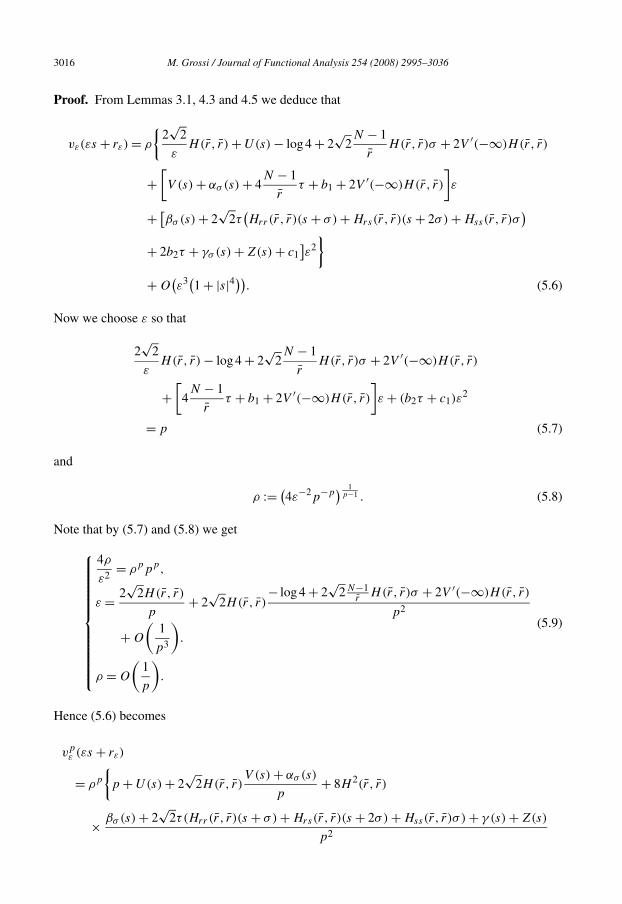
3016 M. Grossi / Journal of Functional Analysis 254 (2008) 2995–3036
Proof. From Lemmas 3.1, 4.3 and 4.5 we deduce that
vε(εs + rε) = ρ
{2√
2
εH(r̄, r̄) + U(s) − log 4 + 2
√2N − 1
r̄H (r̄, r̄)σ + 2V ′(−∞)H(r̄, r̄)
+[V (s) + ασ (s) + 4
N − 1
r̄τ + b1 + 2V ′(−∞)H(r̄, r̄)
]ε
+ [βσ (s) + 2
√2τ
(Hrr(r̄, r̄)(s + σ) + Hrs(r̄, r̄)(s + 2σ) + Hss(r̄, r̄)σ
)+ 2b2τ + γσ (s) + Z(s) + c1
]ε2
}
+ O(ε3(1 + |s|4)). (5.6)
Now we choose ε so that
2√
2
εH(r̄, r̄) − log 4 + 2
√2N − 1
r̄H (r̄, r̄)σ + 2V ′(−∞)H(r̄, r̄)
+[
4N − 1
r̄τ + b1 + 2V ′(−∞)H(r̄, r̄)
]ε + (b2τ + c1)ε
2
= p (5.7)
and
ρ := (4ε−2p−p
) 1p−1 . (5.8)
Note that by (5.7) and (5.8) we get
⎧⎪⎪⎪⎪⎪⎪⎪⎪⎪⎪⎪⎨⎪⎪⎪⎪⎪⎪⎪⎪⎪⎪⎪⎩
4ρ
ε2= ρppp,
ε = 2√
2H(r̄, r̄)
p+ 2
√2H(r̄, r̄)
− log 4 + 2√
2N−1r̄
H (r̄, r̄)σ + 2V ′(−∞)H(r̄, r̄)
p2
+ O
(1
p3
).
ρ = O
(1
p
).
(5.9)
Hence (5.6) becomes
vpε (εs + rε)
= ρp
{p + U(s) + 2
√2H(r̄, r̄)
V (s) + ασ (s)
p+ 8H 2(r̄, r̄)
× βσ (s) + 2√
2τ(Hrr(r̄, r̄)(s + σ) + Hrs(r̄, r̄)(s + 2σ) + Hss(r̄, r̄)σ ) + γ (s) + Z(s)
2
p
M. Grossi / Journal of Functional Analysis 254 (2008) 2995–3036 3017
+ 2√
2H(r̄, r̄)(− log 4 + 2
√2N−1
r̄H (r̄, r̄)σ + 2V ′(−∞)H(r̄, r̄))(V (s) + ασ (s))
p2
+ 2√
2N − 1
r̄H (r̄, r̄)σ + 2V ′(−∞)H(r̄, r̄)p2 (5.10)
+ O
(1
p3
(1 + |s|4))}p
. (5.11)
Using the estimate
(1 + a
p+ b
p2+ c
p3
)p
= ea
[1 + 1
p
(b − a2
2
)+ 1
p2
(c − ab + a3
3+ b2
2+ a4
8− a2b
2
)
+ O
(1 + a5 + b3 + c
p3
)], (5.12)
and observing that
U(s),V (s),Z(s) = O(1 + |s|), α(s), γ (s) = O
(1 + |s|2), β(s) = O
(1 + |s|3),
(5.13)
we have
vpε (s)
= ρppp
{1 + U(s)
p+ 2
√2H(r̄, r̄)
V (s) + α(s)
p2+ 8H 2(r̄, r̄)
× β(s) + 2√
2τ(Hrr(r̄, r̄)(s + σ) + Hrs(r̄, r̄)(s + 2σ) + Hss(r̄, r̄)σ ) + γ (s) + Z(s)
p3
+ O
(1
p4
(1 + |s|4))}p
= ρpppeU(s)
{1 +
(2√
2H(r̄, r̄)(V (s) + α(s)
) − 1
2U2(s)
)1
p
+ 1
p2
[8H 2(r̄, r̄)β(s) + 2
√2τ
(Hrr(r̄, r̄)(s + σ) + Hrs(r̄, r̄)(s + 2σ) + Hss(r̄, r̄)σ
)
+ γ (s) + Z(s) − U(s)(2√
2H(r̄, r̄)V (s) + α(s)) + U3(s)
3+ 2
√2H(r̄, r̄)V (s) + α(s)
2
+ U4(s)
8− U2(s)(2
√2H(r̄, r̄)V (s) + α(s))
2
]+ O
(1
p3
(1 + |s|5))}
. (5.14)
Recalling the equations satisfied by wε , z1,ε , z2,ε and using (5.9) we derive from (5.14)

3018 M. Grossi / Journal of Functional Analysis 254 (2008) 2995–3036
∣∣Rε(s)∣∣ =
∣∣∣∣v′′ε + N − 1
rvε − a(r)vε + vp
ε
∣∣∣∣ = 4ρ
ε2eU(s)O
(1
p3
(1 + |s|5))
= O
(1
p2eU(s)
(1 + |s|5)). (5.15)
Finally, for any α ∈ (0,1),
ε
[(1 + e
√2s)2
e√
2s
]α∣∣Rε(s)∣∣ = O
(1
p3e(1−α)U(s)
(1 + |s|4)) = O
(1
p3
),
and so
‖Rε‖∗ = sups∈(−rε/ε,(1−rε)/ε)
ε
[(1 + e
√2s)2
e√
2s
]α∣∣Rε(s)∣∣ = O
(1
p3
).
This proves our claim. �Lemma 5.2. It holds
pε2(vε(εs + rε))p−1 → eU(s) C1-uniformly on compact sets of R (5.16)
and there exists c > 0 such that
pε2(vε(r))p−1 � ceαU(
r−rεε
) for any r ∈ [0,1], (5.17)
for any α ∈ (0,1).
Proof. The claim (5.16) follows directly by the previous proposition. In order to prove the sec-ond statement we point out that,∣∣W1,σ (s),W3,σ (s)
∣∣ � Cs2 for s large. (5.18)
Then we have that,
fσ (s) � Cs2, gτ (s) � Cs4. (5.19)
We also recall that V (s) and Y(s) growth linearly at infinity. Then, from (5.5) we get
ε
[(1 + es)2
es
]α∣∣Rε(rε + εs)∣∣
= ε
[(1 + es)2
es
]α∣∣∣∣vpε (rε + εs) − 4γ
ε2eU(s)
[1 + ε
(V (s) + f (s)
) + ε2(Y(s) + g(s))]∣∣∣∣
� ‖Rε‖∗ � C
p3. (5.20)
Then,

M. Grossi / Journal of Functional Analysis 254 (2008) 2995–3036 3019
εvpε (rε + εs) � C
p3eαU(s) + CeU(s)
[1 + ε
(V (s) + f (s)
) + ε2(Y(s) + g(s))]
� CeαU(s) (5.21)
for any α ∈ (0,1). Since ε = O( 1p), (5.17) follows. �
6. The invertibility of the linearized operator
In this section we study the linearized problem associated to (1.2). Taking in account(5.7)–(5.9) from now on we write up , vp , φp , Rp instead of uε , vε , φε , Rε . Moreover we havethat up = vp + φp is a solution to
⎧⎪⎨⎪⎩
−u′′ − N − 1
ru + a(r)u = (
u+)p in Ω,
u > 0 in Ω,
u = 0 on ∂Ω
(6.1)
if and only if φp solves the problem
⎧⎨⎩
L(φ) = Nε(φ) + Rp in (0,1),
φ′(0) = 0,
φ(1) = 0,
(6.2)
where
L(φ) := −φ′′ − N − 1
rφ + a(r)φ − pv
p−1p φ, (6.3)
N(φ) := [(vp + φ)+
]p − vpp − pv
p−1p φ (6.4)
and Rp is defined in (5.3).The next results state that the linearized operator L is uniformly invertible (see also [13,
Proposition 3.1] for a related problem).
Theorem 6.1. There exist p0 > 0 and C > 0 such that for any p � p0 and for any h ∈ L∞((0,1))
there exists a unique φ ∈ W2,2((0,1)) solution of
{L(φ) = h in (0,1),
φ′(0) = 0,
φ(1) = 0,
(6.5)
which satisfies
‖φ‖∞ � C‖h‖∗. (6.6)

3020 M. Grossi / Journal of Functional Analysis 254 (2008) 2995–3036
Proof. We argue by contradiction. Assume that there exist sequences pn → +∞, hn ∈L∞((0,1)) and φn ∈ W2,2((0,1)) solutions of
⎧⎪⎨⎪⎩
−φ′′n − N − 1
rφ′
n + a(r)φn − pnvpn−1n φn = hn in (0,1),
φ′n(0) = 0,
φn(1) = 0,
(6.7)
with
vn := γn(wn + εnzn), wn := wεn, zn := zεn (6.8)
and
‖φn‖∞ = 1, ‖hn‖∗ → 0. (6.9)
Let ψn(s) := φn(εns + rn), where rn := rεn = r̄ + σεn + τε2n. Then ψn solves
⎧⎪⎪⎪⎪⎨⎪⎪⎪⎪⎩
−ψ ′′n − N − 1
εns + rnεnψ
′n + ε2
na(εns + rn)ψn − pnε2n
(vn(εns + rn)
)pn−1ψn
= ε2nhn(εns + rn) in
(−rn/εn, (1 − rn)/εn
),
ψ ′n(−rn/εn) = 0,
ψn
((1 − rn)/εn
) = 0.
(6.10)
We point out that ‖ψn‖∞ = 1 and
∥∥ε2nhn(εns + rn)
∥∥∞ � c∥∥εnhn(εns + rn)
∥∥∗ = o(εn).
Then by (6.10) and Lemma 5.2 we get that ψn → ψ C2-uniformly on compact sets of R. More-over ψ solves
{−ψ ′′ − eU(s)ψ = 0 in R,
‖ψ‖∞ � 1.(6.11)
A straightforward computation shows (see [15]) that there exist a and b in R such that
ψ(s) = ae√
2s − 1
e√
2s + 1+ b
(−2 + √
2se√
2s − 1
e√
2s + 1
). (6.12)
It is immediate to check that b = 0, since ‖ψ‖∞ � 1 and then
ψ(s) = ae√
2s − 1
e√
2s + 1. (6.13)
We will show that a = 0. The proof of this claim needs a lot of work. First we prove that
φn(r) → φ0(r) = a(C1G(r, r̄) − 2Gs(r, r̄)
)pointwise in [0,1] \ {r̄}, (6.14)

M. Grossi / Journal of Functional Analysis 254 (2008) 2995–3036 3021
for some real constant C1.In fact, by mean value theorem, we deduce that for any r �= r̄
G(r, εns + rn) = G(r, r̄) + Gs(r, r̄)(s + σ)εn + O(ε2n
(1 + |s|2))
and so, using the smoothness of the Green function for r �= r̄ (see Appendix A), we get
φn(r) =1∫
0
G(r, t)[pn
(vn(t)
)pn−1φn(t) + hn(t)
]dt
= εn
(1−rn)/εn∫−rn/εn
G(r, εns + rn)[pn
(vn(εns + rn)
)pn−1ψn(s) + hn(εns + rn)
]ds
= G(r, r̄)
(1−rn)/εn∫−rn/εn
εnpn
(vn(εns + rn)
)pn−1ψn(s) ds
+ Gs(r, r̄)
(1−rn)/εn∫−rn/εn
ε2npn
(vn(εns + rn)
)pn−1(s + σ)ψn(s) ds
+ O
( (1−rn)/εn∫−rn/εn
ε3npn
(vn(εns + rn)
)pn−1(s + σ)ψn(s)
(1 + |s|2)ds
)
+ εn
(1−rn)/εn∫−rn/εn
G(r, εns + rn)hn(εns + rn) ds. (6.15)
The last integral is estimated as follows:
∣∣∣∣∣εn
(1−rn)/εn∫−rn/εn
G(r, εns + rn)hn(εns + rn) ds
∣∣∣∣∣ � ‖hn‖∗∫R
∣∣G(r, εns + rn)∣∣[ e
√2s
(1 + e√
2s)2
]α
ds
� c‖hn‖∗ = o(1). (6.16)
By Lemma 5.2, we get
(1−rn)/εn∫−rn/εn
ε2npn
(vn(εns + rn)
)pn−1(s + σ)ψn(s) ds
= a√2
∫R
eU(s)(s + σ)U ′(s) ds + o(1) = a√2
∫R
eU(s) + o(1)sU ′(s) ds + o(1)
= −2a + o(1). (6.17)

3022 M. Grossi / Journal of Functional Analysis 254 (2008) 2995–3036
Moreover again by Lemma 5.2 it holds
O
( (1−rn)/εn∫−rn/εn
ε3npn
(vn(εns + rn)
)pn−1(s + σ)ψn(s)
(1 + |s|2)ds
)= o(1). (6.18)
It remains to estimate the integral
(1−rn)/εn∫−rn/εn
εnpn
(vn(εns + rn)
)pn−1ψn(s) ds.
We are not able to valuate it directly, but using (6.15)–(6.18) and the boundedness of φn we get
∣∣∣∣∣(1−rn)/εn∫−rn/εn
εnpn
(vn(εns + rn)
)pn−1ψn(s) ds
∣∣∣∣∣ � C
G(r̂, r̄)
for some r̂ ∈ (0,1), r̂ �= r̄ . Then we have that
(1−rn)/εn∫−rn/εn
εnpn
(vn(εns + rn)
)pn−1ψn(s) ds → C1 as n → ∞,
and it gives the claim (6.14).Note that if a �= 0 by the definition of Green’s function it is easy to verify that φ0 �≡ 0 in (0,1).
So we can assume that φ0 �≡ 0 in (0, r̄) (if φ0 �≡ 0 in (r̄,1) a similar argument applies).Next aim is to construct a suitable test function η which helps to reach a contradiction.Let us fix real numbers 0 < r1 < r̄ < r2 < r3 < 1, a bounded sequence An ∈ R, and let us
introduce the function:
ηn(r) :=
⎧⎪⎪⎨⎪⎪⎩
0, r ∈ (r3,1],e
√2 r−rn
εn −1
e
√2 r−rn
εn +1, r ∈ (r1, r2],
Anr2 + Bnr + Cn, r ∈ [0, r1],
where Bn,Cn ∈ R are chosen so that ηn is a C1-function in [0,1]. We also assume thatηn(r) → η0(r) in C2 for r ∈ (r2, r3). Observing that ηn(r) is differentiable in r = r1 we have
(Anr
2 + Bnr + Cn
) = An(r − r1)2 − 1 + o(1).
We multiply Eq. (6.7) by ηn and we get

M. Grossi / Journal of Functional Analysis 254 (2008) 2995–3036 3023
1∫0
rN−1φ′n(r)η
′n(r) dr +
1∫0
rN−1a(r)φn(r)ηn(r) dr −1∫
0
pnvpn−1n rN−1φn(r)ηn(r) dr
=1∫
0
rN−1hn(r)ηn(r) dr. (6.19)
Let us estimate the four integrals.
I1 =1∫
0
rN−1φ′n(r)η
′n(r) dr
= −1∫
0
rN−1φn(r)η′′n(r) dr − (N − 1)
1∫0
rN−2φn(r)η′n(r) dr
= −2An
r1∫0
rN−1φn(r) dr + 4
ε2n
r2∫r1
rN−1φn(r)e
√2 r−rn
εn
(e
√2 r−rn
εn + 1)2dr −
r3∫r2
rN−1φn(r)η′′n(r) dr
− (N − 1)
r1∫0
rN−2φn(r)(2Anr + B)dr −√
2(N − 1)
εn
r2∫r1
rN−2φn(r)e
√2 r−rn
εn
(e
√2 r−rn
εn + 1)2dr
− (N − 1)
r2∫0
rN−3φn(r)ηn(r) dr
= −2An
r1∫0
rN−1φ0(r) dr + 4
ε2n
r2∫r1
rN−1φn(r)e
√2 r−rn
εn
(e
√2 r−rn
εn + 1)2dr
− 2An(N − 1)
r1∫0
rN−1φ0(r) dr + D1 + o(1), (6.20)
where D1 is a constant independent of An. Then,
I2 =1∫
0
rN−1a(r)φn(r)ηn(r) dr
=r1∫
rN−1a(r)φn(r)(Anr
2 + Bnr + Cn
)dr +
r2∫rN−1a(r)φn(r)
e
√2 r−rn
εn−1
e
√2 r−rn
εn + 1dr
0 r1

3024 M. Grossi / Journal of Functional Analysis 254 (2008) 2995–3036
−r3∫
r2
rN−1a(r)φn(r)ηn(r) dr
=r1∫
0
rN−1a(r)An(r − r1)2φ0(r) dr + D2 + o(1), (6.21)
where D2 is a constant independent of An.
I3 =1∫
0
pnvpn−1n rN−1φn(r)ηn(r) dr =
r2∫r1
pnvpn−1n rN−1φn(r)ηn(r) dr + o(1),
|I4| =∣∣∣∣∣
1∫0
rN−1hn(r)ηn(r) dr
∣∣∣∣∣
=∣∣∣∣∣εn
(1−rn)/εn∫−rn/εn
(εns + rn)N−1hn(εns + rn)ηn(εns + rn) ds
∣∣∣∣∣� ‖hn‖∗
∫R
∣∣η(εns + rn)∣∣[ e
√2s
(1 + e√
2s)2
]α
ds
� c‖hn‖∗ = o(1), (6.22)
because ηn is bounded in [0,1] uniformly with respect to n. From I1, . . . , I4, we get
An
r1∫0
rN−1φ0(r)(N + a(r)An(r − r1)
2)dr + D1 + D2
+r2∫
r1
rN−1φn(r)ηn(r)
(4
ε2n
e
√2 r−rn
εn
(e
√2 r−rn
εn + 1)2dr − pnv
pn−1n
)= o(1). (6.23)
Observe that (5.14) of Lemma 5.1 gives
pnvpn−1n (εns + rn)
= ρpn−1ppneU(s)
[1 +
(2√
2H(r̄, r̄)(V (s) + α(s)
) − 1
2U2(s)
)1
p+ O
(1
p2
(1 + |s|5))]
= 4
ε2n
eU(s)
[1 +
(2√
2H(r̄, r̄)(V (s) + α(s)
) − 1
2U2(s)
)1
p+ O
(1
p2
(1 + |s|5))]
. (6.24)
Rescaling the integral in (6.23) from (6.24) we derive that

M. Grossi / Journal of Functional Analysis 254 (2008) 2995–3036 3025
r2∫r1
rN−1φn(r)ηn(r)
(4
ε2n
e
√2 r−rn
εn
(e
√2 r−rn
εn + 1)2dr − pnv
pn−1n
)
= C
∫R
eU
(2√
2H(r̄, r̄)(V (s) + α(s)
) − 1
2U2(s)
)ds + o(1). (6.25)
Hence (6.23) becomes
An
r1∫0
rN−1φ0(r)(N + a(r)An(r − r1)
2)dr + D = o(1) (6.26)
for some constant D independent of An. Since φ0 �≡ 0 in (0, r0) we can choose An so that
An
r1∫0
rN−1φ0(r)(N + a(r)An(r − r1)
2)dr + D = 1
and this gives a contradiction. Then a = 0 in (6.13).Finally, we prove that a contradiction arises. In fact, by (6.7) we deduce that
φn(r) =1∫
0
G(r, t)[pn
(vn(t)
)pn−1φn(t) + hn(t)
]dt
= εn
(1−rn)/εn∫−rn/εn
G(r, εns + rn)[pn
(vn(εns + rn)
)pn−1ψn(s) + hn(εns + rn)
]ds
= G(r, r̄)
(1−rn)/εn∫−rn/εn
εnpn
(vn(εns + rn)
)pn−1ψn(s) ds
+ εn
(1−rn)/εn∫−rn/εn
[G(r, εns + rn) − G(r, r̄)
]pn
(vn(εns + rn)
)pn−1ψn(s) ds
+ εn
(1−rn)/εn∫−rn/εn
G(r, εns + rn)hn(εns + rn) ds. (6.27)
Let us remark that Lemma A.4 of Appendix A and the definition of the function Γ imply thatthere exists c > 0 such that for any r, s, t ∈ [0,1] it holds∣∣G(r, s) − G(r, t)
∣∣ � c|s − t |. (6.28)
Then by Lemma 5.2 we deduce that, for some α ∈ (0,1),

3026 M. Grossi / Journal of Functional Analysis 254 (2008) 2995–3036
∣∣∣∣∣εn
(1−rn)/εn∫−rn/εn
[G(r, εns + rn) − G(r, r̄)
]pn
(vn(εns + rn)
)pn−1ψn(s) ds
∣∣∣∣∣� c
∫R
|εns + rn − r̄|εnpn
(vn(εns + rn)
)pn−1∣∣ψn(s)∣∣ds
� c
∫R
|s + σ |ε2npn
(vn(εns + rn)
)pn−1∣∣ψn(s)∣∣ds
� c
∫R
|s + σ |eαU(s)∣∣ψn(s)
∣∣ds = o(1), (6.29)
because ψn → 0 pointwise in R and ‖ψn‖∞ � 1. Moreover, by (6.16) we have that
∣∣∣∣∣εn
(1−rn)/εn∫−rn/εn
G(r, εns + rn)hn(εns + rn) ds
∣∣∣∣∣ = o(1). (6.30)
Finally, by (6.27), (6.29) and (6.30) we get for any r ∈ [0,1],
φn(r) = KnG(r, r̄) + o(1),
Kn :=(1−rn)/εn∫−rn/εn
εnpn
(vn(εns + rn)
)pn−1ψn(s) ds, (6.31)
where o(1) is uniform with respect to r ∈ [0,1]. By (6.31) we get φn(rn) = KnG(rn, r̄) + o(1)
and then Kn = o(1), since φn(rn) = ψn(0) = o(1) and G(rn, r̄) → G(r̄, r̄) �= 0, because 0 <
r̄ < 1. A contradiction arises since by assumption ‖φn‖∞ = 1 and by (6.31) it follows that‖φn‖∞ = o(1), because G is a bounded function in [0,1] × [0,1]. �7. The contraction argument
In this section we give the proof of Theorem 1.1. We follow the line of Lemma 4.1 in [13].Let us recall that we are looking for solutions of the type
up = vp + φp. (7.1)
Let us start with the following
Lemma 7.1. We have that
vp(r) > 0 for any r ∈ (0,1), (7.2)
vp(r) → 1G(r, r̄) uniformly in (0,1) (7.3)
H(r̄, r̄)

M. Grossi / Journal of Functional Analysis 254 (2008) 2995–3036 3027
and ∥∥vpp
∥∥∗ � C (7.4)
where C is a positive constant independent of p.
Proof. Let us show that the right-hand side of (5.2) is bounded in L1(0,1). Indeed
4ρ
ε2
1∫0
eUε,rε[1 + ε
(Vε(r) + fε(r)
) + ε2(Zε(r) + gε(r))]
dr
= 4ρ
ε
1−rεε∫
− rεε
eU(s)[1 + ε
(V (s) + f (s)
) + ε2(Z(s) + g(s))]
ds � C
by the polynomial growth of V , Z, f , g and (5.9). Some easy remarks on ODE imply that v′p is
uniformly bounded and it is easy derive that
vp(r) → ξG(r, r̄) uniformly in (0,1). (7.5)
Let us compute ξ ,
ξ = limε→0
4ρ
ε2
1∫0
eUε,rε[1 + ε
(Vε(s) + fε(s)
) + ε2(Zε(s) + gε(s))]
dr
= limε→0
4ρ
ε
1−rεε∫
− rεε
eU(s)[1 + ε
(V (s) + f (s)
) + ε2(Z(s) + g(s))]
ds
= limε→0
4ρ
ε
(∫R
eU(s) + o(1)
)= lim
ε→0
ρ
ε
(2√
2 + o(1)). (7.6)
By (5.9) we derive that limε→04ρε
= 12√
2H(r̄,r̄)which gives (7.3).
Moreover, since we have that vp → G(r, r̄) in C1(r̂,1) for any r̂ > r̄ , the positivity of theGreen function and G(1, s)′ < 0 imply (7.2).
Concerning (7.4), by Lemma 5.2 we get
∥∥vpp
∥∥∗ = sups∈(−rε/ε,(1−rε)/ε)
ε
[(1 + e
√2s)2
e√
2s
]α
vpp(εs + rε)
� cε
pε2
[(1 + e
√2s)2
e√
2s
]α
eαU(s) � C (7.7)
which proves the claim. �

3028 M. Grossi / Journal of Functional Analysis 254 (2008) 2995–3036
Let us write problem (6.2) in the following way,
⎧⎪⎨⎪⎩
−φ′′p − N − 1
rφ′
p + a(r)φp − pvp−1p φ = Rp + Np(φp) in (0,1),
φ′p(0) = 0,
φp(1) = 0,
(7.8)
where Rp is defined in (5.3), (5.9) and
Np(φp) = [(vp + φp)+
]p − vpp − pv
p−1p φp. (7.9)
Proof of Theorem 1.1. Let us denote by C∗ the function space C([0,1]) endowed with thenorm ‖ · ‖∗. By Theorem 6.1 the operator L is uniformly invertible and then there exists L−1,L−1 : C∗ → C([0,1]) such that ‖L−1‖C([0,1]) � C for some positive constant C ∈ R.
Then problem (7.8) can be written in the following way,
φp = T (φ) = −L−1(Rp + Np(φp)). (7.10)
For a given number δ > 0 let us consider the closed set
Aδ ={φ ∈ C(Ω): ‖φ‖∞ � δ
p3
}. (7.11)
We have the following estimates,
∥∥N(φ)∥∥∗ � Cp2‖φ‖2∞, (7.12)∥∥N(φ1) − N(φ2)∥∥∗ � Cp2
(maxi=1,2
‖φi‖∞)‖φ1 − φ2‖∞ (7.13)
for some positive constant C and for any φ1, φ2, φ ∈Aδ .Let us prove (7.12). By mean value theorem we have
∣∣N(φ)∣∣ � p(p − 1)
2
(vp + O
(1
p3
))p−2
φ2 (7.14)
and by (7.2) the claim follows. In the same way (7.13) is proved. Now we are in a position toprove that T is a contraction mapping.
Indeed by (7.12), Theorem 6.1 and Lemma 5.1 we get
∥∥T (φ)∥∥∞ � λ′(∥∥N(φ)
∥∥∗ + ‖Rp‖∗)� O
(p2‖φ‖2∞
) + λ
p3(7.15)
and
∥∥T (φ1) − T (φ2)∥∥∞ � χ
∥∥N(φ1) − N(φ2)∥∥∗ � Cp2
(max‖φ‖∞
)‖φ1 − φ2‖∞ (7.16)
i=1,2

M. Grossi / Journal of Functional Analysis 254 (2008) 2995–3036 3029
for any φ1, φ2, φ ∈Aδ and where λ is independent of δ. Hence, if ‖φ‖∞ � 2λ
p3 we have that, for p
large,
∥∥T (φ)∥∥∞ = O
(1
p4
)+ λ
p3� 2λ
p3. (7.17)
Hence T maps the set {φ ∈ C(Ω): ‖φ‖∞ � 2λ
p3 } in itself. Then T is a contraction mapping on A2λ
since, for p large,
∥∥T (φ1) − T (φ2)∥∥∞ � 1
2‖φ1 − φ2‖∞. (7.18)
Therefore, a unique fixed point φp of T exists in A2λ.Let us prove (1.4). Since up = vp + φp and
‖φp‖∞ � C
ε‖φp‖∗ = O
(1
p2
)(7.19)
it is enough to prove (1.4) for the function vp . Then the claim follows from (7.3) of Lemma (7.1).The proof is finished. �
8. An example of function a(r) satisfying (3.1) and (3.2)
In this section we exhibit a function a(r) which satisfies conditions (3.1) and (3.2).Let ξ ∈ C∞
0 (R), ξ � 0 and ξ �≡ 0, and set
a(r) = aε(r) = 1
εξ
(r − r0
ε
)(8.1)
for some r0 ∈ (0,1). We will show that for ε small enough the function H(ε)(r, s) associatedto aε(r) admits a point r̄ ∈ (0,1) verifying (3.1) and (3.2). We recall that the function H(ε)(r, s)
satisfies
⎧⎪⎪⎪⎨⎪⎪⎪⎩
−H(ε)rr (r, s) − N − 1
rH (ε)
r (r, s) + aε(r)H(ε)(r, s) = −a(r)Γ (r, s), r ∈ (0,1),
H (ε)r (0, s) = 0,
H (ε)(1, s) = 1
N − 2
(s − sN−1).
(8.2)
As we show in Appendix A, H(ε)r (r, s) is uniformly bounded for r ∈ (0,1). Then
H(ε)(r, s) → H 0(r, s) uniformly for r ∈ (0,1).
Moreover, using that aε(r) is compactly supported in (r0 − Mε, r0 + Mε) for some M ∈ R wealso have that H(ε)(r, s) → H 0(r, s) in C2([0,1] \ r0).
Let us compute H 0(r, s). For any φ ∈ C∞(0,1) we have that
0
3030 M. Grossi / Journal of Functional Analysis 254 (2008) 2995–3036
1∫0
(−H(ε)
rr (r, s) − N − 1
rH (ε)
r (r, s)
)φ(r) dr
= −1∫
0
aε(r)rN−1(H(ε)(r, s) + Γ (r, s)
)φ(r) dr
= −1−r0
ε∫− r0
ε
ξ(t)(r0 + εt)N−1(H(ε)(r0 + εt, s) + Γ (r0 + εt, s))φ(r0 + εt) dt
= −rN−10
∫R
ξ(t) dt(H(0)(r0, s) + Γ (r0, s)
)φ(r0) + o(1) (8.3)
as ε → 0. Then H 0(r, s) is the unique solution of the problem
⎧⎪⎪⎪⎨⎪⎪⎪⎩
−H(0)rr (r, s) − N − 1
rH (0)
r (r, s) = βδr0(r), r ∈ (0,1),
H (0)r (0, s) = 0,
H (0)(1, s) = 1
N − 2
(s − sN−1),
(8.4)
where β = −rN−10
∫R
ξ(t) dt (H (0)(r0, s)+Γ (r0, s)). A straightforward computation shows that
H(0)(r, s) = 1
N − 2
(s − sN−1) − β
rN−10
N − 2
{1 − r2−N
0 if r < r0,
1 − r2−N if r � r0.(8.5)
Setting r = r0 in (8.5) we derive
H(0)(r0, s) = s − sN−1 + Γ (r0, s)r2N−20 (1 − r2−N
0 )∫
Rξ(t) dt
N − 2 − r2N−20 (1 − r2−N
0 )∫
Rξ(t) dt
. (8.6)
From (8.6) we get
β −→ (N − 2)Γ (r0, s) + s − sN−1
rN−10 (1 − r2−N
0 )as
∫R
ξ(t) dt → +∞. (8.7)
Finally let us compute H(0)r (r, s). For r > r0 we have that H
(0)r (r, s) = −βrN−1
0 r1−N and thenfor s > r0,
H(0)r (s, s) = −βrN−1
0 s1−N −→ s − sN−1
r0 − rN−10
rN−10 s1−N as
∫ξ(t) dt → +∞. (8.8)
R

M. Grossi / Journal of Functional Analysis 254 (2008) 2995–3036 3031
Since lims→r+0
s−sN−1
r0−rN−10
rN−10 s1−N = 1 there exist at least a point r̄ ∈ (r0,1) for which
H(0)r (r̄, r̄) = 1
2 .Let us show that at r̄ the condition (3.2) is verified. From the definition of H(0)(r, s) we have
that H(0)rs (r̄, r̄) = 0 since r̄ > r0. Moreover
H(0)rr (r̄, r̄) = (N − 1)βrN−1
0 r̄−N �= 0
which proves the claim.
Appendix A. Some remarks on Green’s function
In this appendix we sketch some properties of Green’s function G(r, s) of the operator
−u′′ − N − 1
ru′ + a(r)u, r ∈ (0,1).
It is possible that these results are known but, since we are not able to provide any reference, wegive them a proof. The argument is quite elementary. Let N � 3. By definition, for any smoothfunction f , we have that
v(r) =1∫
0
G(r, s)f (s) ds
is the unique solution of the problem
{−u′′ − N − 1
ru′ + a(r)u = f in (0,1),
u′(0) = u(1) = 0.
Let us introduce the function
Γ (r, s) = sN−1
2(N − 2)
(r2−N − s2−N − ∣∣r2−N − s2−N
∣∣)
={
0 if r < s,sN−1
N−2 (r2−N − s2−N) if r > s(A.1)
for r, s ∈ (0,1). It is easy to check that Γ (r, s) verifies
{−Γrr(r, s) − N − 1
rΓr(r, s) = δs(r), r ∈ (0,1),
Γr(0, s)(0) = 0
in the sense of distributions. Here δs(r) is the Dirac function centered at s. Then we have thefollowing decomposition for Green’s function,
G(r, s) = Γ (r, s) + H(r, s), (A.2)
3032 M. Grossi / Journal of Functional Analysis 254 (2008) 2995–3036
where H(r, s) is the solution of the problem
⎧⎪⎪⎪⎨⎪⎪⎪⎩
−Hrr(r, s) − N − 1
rHr(r, s) + a(r)H(r, s) = −a(r)Γ (r, s), r ∈ (0,1),
Hr(0, s) = 0,
H(1, s) = 1
N − 2
(s − sN−1).
(A.3)
H(r, s) is called the regular part of Green’s function; we point out that H(r, s) is uniformlybounded in (0,1) with respect to s. Indeed by standard maximum principle we have thatH(r, s) > 0 in (0,1). Let us prove that H(r, s) is bounded from above uniformly with respectto s. Multiplying (A.3) by rN−1 and integrating we get
Hr(r, s)rN−1 =
r∫0
aε(t)tN−1(H(t, s) + Γ (t, s) dt
)dt
=r∫
0
aε(t)tN−1G(t, s) dt > 0. (A.4)
Hence H(r, s) is strictly increasing in r and then
H(r, s) < H(1, s) = 1
N − 2
(s − sN−1),
which gives the claim.Hence, by the definition of G(r, s), we derive that Green’s function is bounded in [0,1]. We
have the following
Lemma A.1. Green’s function G(r, s) satisfies
G(r, s)rN−1 = G(s, r)sN−1. (A.5)
Proof. It is enough to repeat step by step the proof in [10]. �Corollary A.2. The following identities hold:
H(s, r) = H(r, s)rN−1
sN−1+ rN−1
N − 2
(r2−N − s2−N
), 0 � r, s � 1,
Hs(t, t) = Hr(t, t) + H(t, t)N − 1
t− 1, 0 � y � 1. (A.6)
Proof. It follows by the previous lemma and by the decomposition G(r, s) = Γ (r, s) +H(r, s). �

M. Grossi / Journal of Functional Analysis 254 (2008) 2995–3036 3033
Corollary A.3. Let F(r) = H(r,r)
rN−1 . We have that
F ′(r̄) = 0 ⇔ Hr(r̄, r̄) = 1
2
and
F ′′(r̄) �= 0 ⇔ Hrr(r̄, r̄) + Hrs(r̄, r̄) �= 0.
Proof. The proof follows by a straightforward computation using Corollary A.2. �Next lemma deals with the smoothness of the regular part H(r, s).
Lemma A.4. The regular part of Green’s function H(r, s) satisfies
H(r, s) ∈ C2([0,1] × [0,1]). (A.7)
Moreover we have that, for r �= s,
H(r, s) ∈ C3([0,1] × [0,1]), (A.8)
and there exist the limits
H+rrr = lim
(r,s)→(r̄,r̄)Hrrr (r, s) for r > s (A.9)
and
H−rrr = lim
(r,s)→(r̄,r̄)Hrrr (r, s) for r < s. (A.10)
The same happens for the derivatives Hrrs , Hrsr , Hrss , Hssr , Hsss .
Proof. By classical results for ordinary differential equations we have that H(r, s) is differen-tiable twice in the variable r . Moreover, differentiating Eq. (A.3) with respect to r we get
−Hrrr − N − 1
rHrr + N − 1
r2Hr + ar(r)H + a(r)Hr = 0 for r < s,
−Hrrr − N − 1
rHrr + N − 1
r2Hr + ar(r)H + a(r)Hr = −sN−1r1−N for r > s.
Then (A.8)–(A.10) follow. Now we have to prove the same result for the other derivatives. Wejust show the claim for Hsss (the computation in the other cases is similar).
Since the function H(r, s) − 1 (s − sN−1) vanishes at r = 1, we have
N−2
3034 M. Grossi / Journal of Functional Analysis 254 (2008) 2995–3036
H(r, s) = s − sN−1
N − 2−
1∫0
G(r, t)a(t)
(s − sN−1
N − 2+ Γ (t, s)
)dt
= s − sN−1
N − 2− s − sN−1
N − 2
1∫0
G(r, t)a(t) dt − sN−1
N − 2
1∫s
G(r, t)a(t)(t2−N − s2−N
)dt.
(A.11)
In order to prove our claim is enough to study the last integral. Note that
d
ds
( 1∫s
G(r, t)a(t)(t2−N − s2−N
)dt
)= (N − 2)
1∫s
G(r, t)a(t)s1−N dt. (A.12)
Differentiating again with respect to s we have
d2
ds2
( 1∫s
G(r, t)a(t)(t2−N − s2−N
)dt
)
= (N − 2)(1 − N)s−N
1∫s
G(r, t)a(t) dt − (N − 2)s1−NG(r, s)a(s). (A.13)
Since G(r, s) is a differentiable function in (0,1)× (0,1) for r �= s we have that there exists Hsss
and this is continuous function. On the other hand, since
lim(r,s)→(r̄,r̄)
Gs(r, s) = 1 + Hs(r̄, r̄) for r > s (A.14)
and
lim(r,s)→(r̄,r̄)
Gs(r, s) = Hs(r̄, r̄) for r < s (A.15)
the claim follows. �We now prove some identities which are used in Section 8.
Lemma A.5. We have that
Hr(s, s) =∫ s
0 a(t)tN−1H(t, s) dt
sN−1. (A.16)
for any t ∈ (0,1).

M. Grossi / Journal of Functional Analysis 254 (2008) 2995–3036 3035
Proof. By the definition of H(r, s) we get
−(Hr(r, s)r
N−1)′ + a(r)rN−1H(r, s) = −a(r)rN−1Γ (r, s)
and integrating from 0 to r we have
−Hr(r, s)rN−1 +
r∫0
a(t)tN−1H(t, s) dt = −r∫
0
a(t)tN−1Γ (t, s)
= −r∫
s
a(t)tN−1Γ (t, s). (A.17)
Setting r = s in (A.17) the claim follows. �Lemma A.6. We have that
Hr(1,1) = 0. (A.18)
Proof. By the previous proposition we derive that
Hr(1,1) =1∫
0
a(t)tN−1H(t,1) dt. (A.19)
On the other hand, by Corollary A.2 we deduce that
H(t,1) = H(1, t)1
tN−1+ 1
N − 2
(1 − t2−N
)
and recalling that H(1, t) = 1N−2 (t − tN−1) we get H(t,1) = 0 for any t ∈ (0,1). So the claim
follows. �Proposition A.7. Let us suppose that there exists r̃ ∈ (0,1) such that Hr(r̃, r̃) > 1
2 . Then thereexist at least two points r̄1, r̄2 ∈ (0,1) for which Hr(r̄1, r̄1) = Hr(r̄2, r̄2) = 1
2 .
Proof. Since Hr(0, s) = 0 for any s ∈ (0,1), the smoothness of H implies that Hr(0,0) = 0.From the previous corollary we also get that Hr(1,1) = 0. Then, again using the smoothnessof H , if there exists r̃ ∈ (0,1) such that Hr(r̃, r̃) > 1
2 we derive the existence of at least twopoints r̄1, r̄2 ∈ (0,1) for which Hr(r̄1, r̄1) = Hr(r̄2, r̄2) = 1
2 . �References
[1] A. Bahri, J.M. Coron, On a nonlinear elliptic equation involving the critical Sobolev exponent: The effect of thetopology of the domain, Comm. Pure Appl. Math. 41 (1988) 253–294.
[2] M. Ben Ayed, K. El Mehdi, M. Grossi, O. Rey, A nonexistence result of single peaked solutions to a supercriticalnonlinear problem, Commun. Contemp. Math. 5 (2003) 179–195.

3036 M. Grossi / Journal of Functional Analysis 254 (2008) 2995–3036
[3] H. Brezis, L. Nirenberg, Positive solutions of nonlinear elliptic equations involving critical Sobolev exponents,Comm. Pure Appl. Math. 36 (1983) 437–477.
[4] J.M. Coron, Topologie et cas limite des injections de Sobolev, C. R. Acad. Sci. Paris Sér. I Math. 299 (1984)209–212 (in French).
[5] M. del Pino, J. Wei, Supercritical elliptic problems in domains with small holes, Ann. Inst. H. Poincaré 24 (2007)507–520.
[6] M. del Pino, J. Dolbeault, M. Musso, “Bubble-tower” radial solutions in the slightly supercritical Brezis–Nirenbergproblem, J. Differential Equations 193 (2003) 280–306.
[7] M. del Pino, P. Felmer, M. Musso, Two-bubble solutions in the super-critical Bahri–Coron’s problem, Calc. Var.Partial Differential Equations 16 (2003) 113–145.
[8] M. del Pino, J. Dolbeault, M. Musso, The Brezis–Nirenberg problem near criticality in dimension 3, J. Math. PuresAppl. 83 (2004) 1405–1456.
[9] M. del Pino, M. Kowalczyk, M. Musso, Singular limits in Liouville-type equations, Calc. Var. Partial DifferentialEquations 24 (2005) 47–81.
[10] E. Di Benedetto, Partial Differential Equations, Birkhäuser Boston, Boston, MA, 1995.[11] O. Druet, Elliptic equations with critical Sobolev exponents in dimension 3, Ann. Inst. H. Poincaré 19 (2002) 125–
142.[12] P. Esposito, M. Grossi, A. Pistoia, On the existence of blowing-up solutions for a mean field equation, Ann. Inst.
H. Poincaré 22 (2005) 227–257.[13] P. Esposito, M. Musso, A. Pistoia, Concentrating solution for a planar elliptic problem involving nonlinearities with
large exponent, J. Differential Equations 227 (1) (2006) 29–68.[14] Y. Ge, R. Jing, F. Pacard, Bubble towers for supercritical semilinear elliptic equations, J. Funct. Anal. 221 (2005)
251–302.[15] M. Grossi, Asymptotic behaviour of the Kazdan–Warner solution in the annulus, J. Differential Equations 223
(2006) 96–111.[16] J.L. Kazdan, F.W. Warner, Remarks on some quasilinear elliptic equations, Comm. Pure Appl. Math. 28 (1975)
567–597.[17] R. Molle, A. Pistoia, Concentration phenomena in elliptic problems with critical and supercritical growth, Adv.
Differential Equations 8 (2003) 547–570.[18] D. Passaseo, Nonexistence results for elliptic problems with supercritical nonlinearity in nontrivial domains,
J. Funct. Anal. 114 (1993) 97–105.[19] D. Passaseo, Nontrivial solutions of elliptic equations with supercritical exponent in contractible domains, Duke
Math. J. 92 (1998) 429–457.[20] D. Passaseo, Some sufficient conditions for the existence of positive solutions to the equation −�u+a(x)u = u2∗−1
in bounded domains, Ann. Inst. H. Poincaré 13 (1996) 185–227.[21] A. Pistoia, O. Rey, Multiplicity of solutions to the supercritical Bahri–Coron’s problem in pierced domains, Adv.
Differential Equations 11 (2006) 647–666.[22] S. Pohozaev, Eigenfunctions of the equation �u + λf (u) = 0, Soviet Math. Dokl. 6 (1965) 1408–1411.

![The Brezis–Nirenberg problem for the fractional p-Laplacianmy.fit.edu/~kperera/PDF/MR3530213.pdf · linking was used in Degiovanni and Lancelotti [15]. Moreover, the standard sequence](https://static.fdocuments.net/doc/165x107/5c71db4809d3f25c278b7373/the-brezisnirenberg-problem-for-the-fractional-p-kpererapdfmr3530213pdf.jpg)
![Analisi Funzionale Teoria e Applicazioni [Haim Brezis]](https://static.fdocuments.net/doc/165x107/577cc6ab1a28aba7119ed889/analisi-funzionale-teoria-e-applicazioni-haim-brezis.jpg)