Radial mode decomposition of sound fields in flow ducts...

Radial mode decomposition of sound fields in flow ductsunder consideration of a rigid body like swirl

M. Spitalny 1, U. Tapken 1, C. Faustmann 2, L. Enghardt 1

1 German Aerospace Center, Institute of Propulsion Technology - Engine Acoustics,Mueller-Breslau-Str. 8, D-10623, Berlin, Germanye-mail: [email protected]

2 Graz University of Technology, Institute for Thermal Turbomachinery and Machine Dynamics,Inffeldgasse 25 A, A-8010, Graz, Austria

AbstractRadial mode decomposition is a well-established analysis method to quantify the sound power that is trans-ported by acoustic waves in flow ducts. Furthermore, it enables insight into the sound generation and trans-mission processes of a turbo-machine. The mean flow can have a significant influence on the mode shapefunctions in the propagating sound field. Hence, it has to be considered in the governing equations. Inthe simplest case, the axial component of the flow is modelled as a constant velocity profile (plug flow).The circumferential flow component can be approximately modelled by a rigid body rotation. Applyingthese assumptions, the wave equation can still be solved analytically. The consideration of more complexflow features would require the derivation of the mode shape functions with the help of extensive numericalcalculations. In the present study, the mode decomposition method using the rigid-body-swirl model wasapplied to measurements taken at a two-stage two-spool counter rotating turbine rig (Transonic Test TurbineFacility (TTTF) of Graz University of Technology). In this rig there are no exit guide vanes installed, so thata strong circumferential flow component was present in the acoustic measurement section. The circumfer-ential flow component exhibited up to half of the magnitude of the axial velocity. An array of 24 wall-flushmounted microphones was used to acquire the sound field in the exhaust duct. In order to achieve a sufficientspatial resolution, the array was traversed in steps of two degrees over the whole circumference. Before thecalculation of the frequency spectra, the time signals of all microphones were adaptively resampled withrespect to the rotor shaft trigger in order to eliminate the impact of shaft speed variations. The radial modeamplitudes were determined for the harmonics of the Blade Passing Frequency (BPF) by solving a linearsystem of equations using a singular value decomposition algorithm. In the analysis, the strength of the rigidbody like swirl was varied systematically. The study revealed a significant impact of the model parameters,i.e. mode phase speed and swirl rotational frequency, on the derived sound power of individual modes.

1 Introduction

Future aero engines will have to meet strict requirements regarding their environmental impact. This includesfuel efficiency and reduced NOx-emissions as well as a low noise level. Advanced engine designs demandan improvement in the analysis techniques as the measurements are performed under more challenging con-ditions and refined results are required for further developments. As modern aero engines feature a highlythree-dimensional flow field, this has to be considered when analysing the propagation of sound through theengine duct. The axial component of the flow is usually approximated by a constant flow profile (plug flow).The same is done here. This paper focuses on how the circumferential velocity component affects the radial

345

mode analysis.

In literature, different models for the radial profile of the circumferential velocity component are discussedin theory [10], [13], [11]. The most commonly used models are:

• rigid body rotation

• constant circumferential velocity

• potential swirl (free vortex swirl)

• a combination of those listed above

With a combination of a rigid body rotation and a potential swirl component, the circumferential flow profilesin turbine ducts can be reproduced with a small fit error. But this comes with the cost of losing the abilityto solve the wave equation for cylindrical ducts analytically. The use of the rigid body rotation swirl alonehas the advantage to be the only known swirl model for which an analytical solution of this equation exists.Therefore, no numerical approximation is necessary. This allows an easy incorporation into the existing anal-ysis chain, which has been proven and tested in numerous previous studies [7], [8], [5]. An application of aradial mode analysis with the rigid body rotation model to experimental data was presented by Taddei[12].

The rigid body rotation like swirl can be incorporated in the wave equation by just a single parameter,the rotational frequency Ω of the rigid body rotation. Here, three methods are presented to determine therotational frequency on the basis of aerodynamic respectively acoustic data.Acoustic data from a two-stage two-spool counter rotating turbine rig (Transonic Test Turbine Facility(TTTF)) has been analysed for this purpose. This rig features a state of the art turbine geometry. In theacoustic measurement section a strong circumferential velocity component, with a magnitude of up to 50%of the axial velocity, is present. These conditions are used as a test case for a radial mode analysis includinga swirl model.

2 Theoretical background

In order to perform an azimuthal or radial mode analysis, frequency spectra of the rotor coherent acousticfield are required. Following this analysis step, a sound field model is fitted to the spectral data usingmathematical methods, which are explained in this section.

2.1 Azimuthal mode analysis

The azimuthal mode analysis (AMA) is a spatial Discrete Fourier transform (DFT) performed at a certainfrequency along the circumference of a cylindrical duct. It does not incorporate any assumptions regardingthe flow field or the radial shape of the sound field. The sound pressure amplitudes Am of the azimuthalmodes can be calculated using equation 1. The number of measurement positions N determines how manyazimuthal mode orders m can be resolved. According to the Nyquist-Shannon sampling theorem, there canbe |m| = N/2 azimuthal mode orders without alialising. p(ϕj) is the complex pressure amplitude at thecircumferential position ϕj . This pressure amplitude is extracted from the adaptive frequency spectrum at apoint of interest, usually the blade passing frequency of a rotor.

Am =1

N

N∑j=1

p(ϕj)eimϕj (1)

By means of an azimuthal mode analysis, the dominant spatial structures of a sound field can be identified.These can be used as a reference for the interpretation of the radial mode analysis.

346 PROCEEDINGS OF ISMA2014 INCLUDING USD2014

2.2 Description of mode propagation

The radial mode analysis (RMA) is a commonly used method to assess the sound field in cylindrical ductswith and without a hub. The wave equation in cylindrical coordinates is the basis for this analysis (equation2). It has an analytical solution for the pressure, which is expressed in equation 3[1]:

1

c2

∂2p

∂t2− 1

r

∂

∂r

(r∂p

∂r

)− 1

r2

∂2p

∂ϕ2− ∂2p

∂x2= 0 (2)

Under the constraints of incompressible and isentropic flow, a constant axial mean fow profile, and stationarymean temperature and density, the solution of the convective Helmholtz equation in cylindrical coordinatesis given by a linear superposition of modal terms [6] as follows:

p(x, r, ϕ) =

∞∑m=−∞

∞∑n=0

(A+mn · eik

+mnx +A−mn · eik

−mnx)· fmn(r) · eimϕ (3)

Here, k+mn and k−mn denote the axial wave numbers, A+

mn and A−mn the complex amplitudes of the modewith the azimuthal orderm, and the radial order n for propagation in and against flow direction, respectively.In the case of hard-walled acoustic boundary conditions, the modes form an orthogonal eigensystem. Themodal shape factors are given by fmn(r) = (Fmn)−

12 (Jm(γmn

rR)+QmnYm(γmn

rR), with Jm and Ym being

the Bessel functions of first and second kind and ordermwith associated hard-walled cylindrical eigenvaluesγmn and Qmn. The eigenvalues depend on the hub-to-tip ratio η. Qmn is zero for non-annular cylinders; Ris the outer duct radius. The definition of the normalization factor Fmn is given in [7]. In a hard walled duct,the sound power is solely transported in axial direction. The sound power carried by each individual modecan be calculated according to Morfey [9] as

P±mn =πR2

ρc

αmn(1−M2x)2

(1∓ αmnMx)2

∣∣A±mn∣∣2 , (4)

with αmn =√

(1− (1−M2)(σmn/(kR))2).

2.3 Incorporation of a rigid body rotation like swirl in the radial mode analysis

Flow fields in modern turbo-machines exhibit complex flow profiles. The influence of these flow fields onthe acoustic perturbation has to be modelled in the radial mode analysis.An example for these flow profiles in form of a radial distribution of the circumferential velocity componentis depicted in figure 3. To account for a flow field, the wave equation (2) can be extended by extra terms fora plug flow and a rigid body rotation. Using these models, the equation remains analytically solvable.It isassumed, that in the steady flow field the swirl can be approximated by a rigid body swirl, Uϕ(r) = Ω

r , andthat the flow is uniform in axial direction, Ux = const. The frame of reference with respect to the directionof rotation for the swirl and the spinning mode is equal. If further |Ωω | << 1, i.e. the acoustic frequencyis much higher than the rotation frequency of the swirl, then, as shown by Heinig[15], the terms 2Ωuϕ and2Ωur due to Coriolis forces in the momentum equations can be neglected. Under these assumptions thehomogenous convective Helmholtz equation can be expressed as equation 6.

k2p+ 2ikMx∂p

∂x+ 2ik

Ω

c

∂p

∂ϕ+(1−M2

x

) ∂2p

∂x2+ . . . (5)(

1

r2− Ω2

c2

)∂2p

∂ϕ2− 2Mx

Ω

c

∂

∂x

∂p

∂ϕ+

1

r

∂

∂r

(r∂p

∂r

)= 0

AEROACOUSTICS AND FLOW NOISE 347

The homogenous convective Helmholtz equation expressed as in equation 6 is solved by harmonic relationfor the pressure from equation 3. The influence of a swirl in form of a rigid body rotation on the axialwavenumber kmn depends on its rotational frequency Ω. With this model for the swirl, the axial wavenumberis given by equation 9.

k0 =2πf

c0(6)

k0 =2πf

c0

√1 +

κ− 1

2M2x (7)

k = k0 −mΩ

c0(8)

k±mn =k

1−M2x

−Mx ±

√1− (1−M2

x)

(σmn

kR

)2 (9)

How the wavenumber changes according to equation 9, when a rotational frequency Ω is given is shown infigure 1. Only wavenumbers which are cut-on are plotted. The term cut-on expresses that a certain mode(m,n) is propagating without attenuation. The displayed values of Ω correspond to the determation processexplained in section 4.2.

Figure 1: Changes in the axial wavenumber due to changes in the rotational frequency Ω of the rigid bodyswirl model.


2.4 Radial mode analysis method

The determination of the radial mode spectrum can be regarded as an inverse problem, i.e. the solution isdeduced by means of an inversion of the matrixW relating the vector p of measured complex sound pressurevalues to the vector A of radial mode amplitudes:

p = W ·A. (10)

In most applications, this system has more parameters than unknowns. The dimension of the vector p is givenby the number of measurement positions, which in general is Npos = NxNrNφ and the dimension of A isgiven by the total number of up- and downstream propagating modes Nmodes. Accordingly, the dimensionof W is Npos×Nmodes. A linear least squares fit, e.g. by deploying the pseudo-inverse of matrix W , can beused to determine the radial mode amplitudes:

A =[WHW

]−1WH · p. (11)

The resulting mode amplitude vector minimizes the cost function J = ‖e‖ = ‖WA− p‖, where ‖‖ denotesthe 2-norm. The complex vector of errors ‖e‖ represents noise due to e.g. turbulent pressure fluctuationsas well as an inappropriate description of the mode propagation in the flow duct by the utilized analyticalmodel.

3 Experimental setup and aerodynamic characteristic of the rig

The Transonic Test Turbine Facility (TTTF) is a continuously operating two-stage cold-flow open-circuitplant, which consists of a transonic HPT stage and a counter-rotating LPT stage. This unique configurationallows the testing of rig inserts with a diameter up to 800 mm under engine-representative conditions. Bothturbines are designed with overhung-type turbine shafts and additionally the LPT is mounted on an axiallymoveable frame. This allows for an easy disk assembly without dismantling the bearings. Rather quickand simple rig modifications between setups with transition duct and turning mid turbine frame designs ofdifferent axial lengths are possible. The facility is driven by pressurized air delivered by a separate 3 MWcompressor station. The shaft power of the HP turbine stage drives a three-stage radial brake compressor.This brake compressor delivers additional air mixed to the flow from the compressor station and increasesthe overall mass flow. The air temperature at the turbine stage inlet can be adjusted by coolers between 40

C to 185 C. The maximum shaft speed of the HPT stage is limited to 11550 rpm. Depending on the stagecharacteristics, a maximum coupling power of 2.8 MW at a total mass flow of 22 kg/s can be reached. Thepower of the LP turbine is absorbed by a water brake with a maximum power of 700 kW. Further details onthe transonic test turbine facility (TTTF) can be found in Lengani et. al [4] and Faustmann et. al [5].

Between the rotor in the low pressure part of the turbine and the acoustic measurement section, there is nostator installed (see figure 2). This results in a strong circumferential velocity component (swirl) in this partof the rig. A flow profile for the circumferential component is shown in figure 3. It has been measured at theentrance of the microphone section. The measurement position is marked by a red line in figure 2. The 12microphones set up in the upstream section of the microphone array are installed in a part of the duct withnon-cylindrical geometry. These are followed by 12 microphones in a cylindrical part of the rig.

3.1 Instrumentation

The acoustic test section is equipped with 24 wall-flush mounted microphones in an axial arrangement. Themicrophone array can be traversed by 360 degrees. This is necessary to establish a grid of measurement


Figure 2: Cross-sectional view of the TTTF rig with acoustic and aerodynamic measurement positions

Blade row S1 R1 S2 R2 S3Blade count 24 36 16 72 8

Table 1: TTTF rotor and stator stages with corresponding blade counts

positions with sufficient spatial resolution to perform a radial mode analysis at the blade passing frequenciesof the rotors. A circumferential spacing of 2 was chosen for the traverse steps. The axial spacing in thedownstream part of the microphone array (12 microphones) was 5mm. This dense spacing is achievedby staggering every second microphone by 6 in circumferential direction. Furthermore, a one-pulse perrevolution signal from each rotor shaft was acquired. Microphone and rotor shaft trigger signals have beensampled with 60 kHz. For each microphone position, a time series with a length of 20 seconds was recorded.

3.2 Test point conditions

For the present study, the test point approach was chosen, because it shows up characteristic Tylor Sofrinmodes and has a circumferential velocity component which is up to 50% of the azimuthal velocity compo-nent. The approach case is part of most performed turbine tests, as it represents an operation point that isused in the certification process of an engine. Further information regarding this test point can be found inLengani et. al. [4] and Faustmann et. al. [5].

3.3 Aerodynamic profiles

Figure3 shows the circumferential velocity component in the acoustic measurement section of the TTTF rig.

3.4 Rotor-stator interaction

According to the blade count of the stages of the TTTF listed in table 1, certain modes are predicted by theTylor-Sofrin model[6]. These azimuthal modes (m) can be calculated utilizing equation 12.


Figure 3: Circumferential velocity component measured in the plane marked by a red line in figure 2. Inaddition, the circumferential velocity component for the rigid body rotation swirl is given by the dashed linesfor different values of the rotational frequency Ω.

m = hR− kS (12)

In equation 12, R is the number of rotor blades and S is the number of stator vanes. The azimuthal modespredicted for the high pressure rotor are listed in table 2. h is the rotor harmonic and k is an integer withpositive or negative sign. Due to the used system of coordinates and the rotational direction of the rotor hhad to be negated.

Interaction R1→S2 R1→S1 S1→R1 S2→R1 R1→R2Mode order m +28, +12, -4, -20 +12, -12 +12, -12 +12, -4, -20 +36

Table 2: Modes generated by rotor-stator stages in TTTF

In addition to that, a scattering of modes m = +12 and m = -12 at the S2 stage is expected. This results in themodes +36, +20, +4, -12, -28, -44 and +44, +28, +12, -4, -20, -36, respectively. This scattering is predictedby the following equation [14]:

ms = m− kS (13)

4 Results

In order to examine the effect of the strength of the rotational frequency Ω given in the rigid body rotationmodel, the microphone signals coherent to the high pressure part of the turbine have been analysed. Here, astrong influence of the swirl can be assumed from the measured flow profiles.To reduce the complexity and to focus on the effect of the rotational frequency, only the results for the down-stream propagating modes are shown. The results for the upstream direction exhibit an analogue behaviour.


The mode analyses have been carried out at the blade passing frequency (BPF) of the high pressure turbinerotor.

4.1 Sound pressure spectrum and azimuthal mode analysis

The sound pressure spectrum shown in figure 4 is calculated from sound pressure time signals that have beenadaptively resampled to a one pulse per revolution trigger of the high pressure turbine shaft. In the processof adaptive resampling the time signals of microphone measurements are interpolated equidistantly betweenthe trigger pulses of the rotor shaft (one pulse per revolution). These resampled signals are in turn convertedinto the frequency domain by a Fourier transformation. For each microphone signal this is done for 33 timewindows, the Fourier transform of which are phase-locked averaged in reference to the trigger signal of arotor shaft to increase the signal to noise ratio of the frequency spectra. The spectra have been averaged over180 circumferential traverse steps and 12 axial positions in the downstream part of the array, where the ductsection is cylindrical. These circumferential and axial measurement positions build the grid which is used inthe radial mode analysis.

Figure 4: Averaged spectrum of microphone time signals, which have been adaptively resampled to a onepulse per revolution trigger of the high pressure turbine shaft.

At engine order 36 in figure 4 (the first blade passing frequency of the high pressure turbine rotor) a strongpeak can be seen. This peak has a 30 dB offset to the general noise floor at the surrounding frequencies.Here, tonal noise can be identified as the major sound source. The azimuthal and radial mode analysis isdone on the basis of the complex amplitudes at this frequency. The first harmonic of the BPF can be seen atengine order 72.

In figure 5 the results of an azimuthal mode decomposition are depicted. Mode orders that can be related tothe interaction of blade rows (see section 3.4) are identified by arrows.

4.2 Determination of the rotational frequency Ω for the rigid body swirl model

In this section three different ways to derive a rotational frequency for the analysis are presented. These are:

• circumferential velocity at the outer duct wall


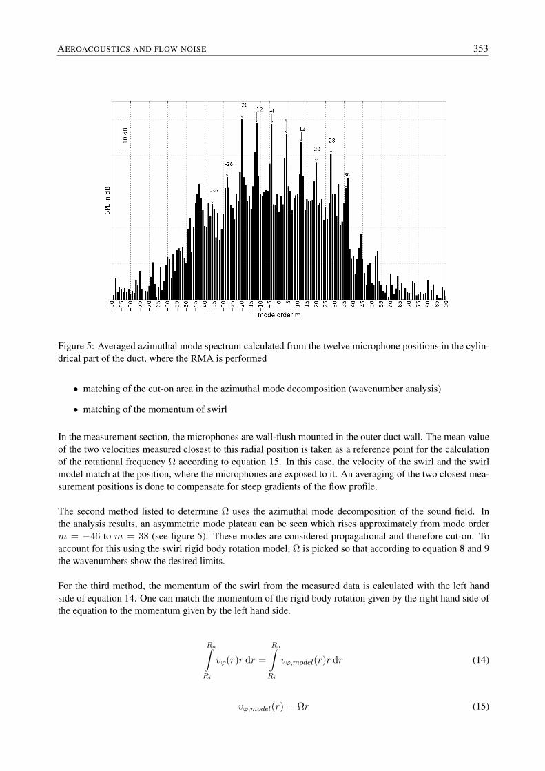
Figure 5: Averaged azimuthal mode spectrum calculated from the twelve microphone positions in the cylin-drical part of the duct, where the RMA is performed

• matching of the cut-on area in the azimuthal mode decomposition (wavenumber analysis)

• matching of the momentum of swirl

In the measurement section, the microphones are wall-flush mounted in the outer duct wall. The mean valueof the two velocities measured closest to this radial position is taken as a reference point for the calculationof the rotational frequency Ω according to equation 15. In this case, the velocity of the swirl and the swirlmodel match at the position, where the microphones are exposed to it. An averaging of the two closest mea-surement positions is done to compensate for steep gradients of the flow profile.

The second method listed to determine Ω uses the azimuthal mode decomposition of the sound field. Inthe analysis results, an asymmetric mode plateau can be seen which rises approximately from mode orderm = −46 to m = 38 (see figure 5). These modes are considered propagational and therefore cut-on. Toaccount for this using the swirl rigid body rotation model, Ω is picked so that according to equation 8 and 9the wavenumbers show the desired limits.

For the third method, the momentum of the swirl from the measured data is calculated with the left handside of equation 14. One can match the momentum of the rigid body rotation given by the right hand side ofthe equation to the momentum given by the left hand side.

Ra∫Ri

vϕ(r)r dr =

Ra∫Ri

vϕ,model(r)r dr (14)

vϕ,model(r) = Ωr (15)


The integrals in equation 14 are within the boundaries of the inner Ri and outer Ra duct wall. The cir-cumferential velocity component is given by vϕ. In case of a neglectable circumferential flow component,characteristic cut-on modes are distributed symmetrically around mode m = 0. Otherwise the distribution isasymmetrical.

Determination method Solid body rotation fre-quency in rad/s

min(m) max(m)

no swirl 0 -42 42circumferential velocity at the outer duct wall 58 -45 39matching of cut-on area in azimuthalmode decomposition

86 -46 38

matching of momentum of swirl 117 -48 37

Table 3: Azimuthal mode orders that are cut-on in the flow duct at different rotational frequencies of therigid body rotation like swirl. The rotational frequencies were determined using different criteria.

Table 3 lists the cut-on modes calculated on the basis of rotational frequencies used in the radial modeanalysis.

4.3 Radial mode analysis with rigid body like swirl

Figure 6: Change of the sound power level with a continuous variation of the rotational frequency Ω. Thesound power level for downstream propagating modes is plotted for the azimuthal mode order m as a sumover the radial orders n.

As mentioned above, radial mode analyses with a countinuous variation of the swirl have been carried out.The results are plotted in figure 6. The colours represent a dynamic range of 45 dB. In the white area of theplot the modes are cut-off. The stepped edges of the cut-on area can be associated with the variation in the


wavenumbers shown in figure 1 and maximum und minimum cut-on mode orders m listed in table 3. Thesteps within the coloured cut-on area for example seen around mode order m=-40 show the cut-on behaviourof higher radial mode orders. If there are no modes becoming cut-on or -off the sound power level changessmoothly.

Figure 7: Change in dB of the Tylor Sofrin modes due to swirl in relation to the case without swirl

Certain modes shown in figure 7 exhibit an abrupt rise in their sound power level. Modes of low azimuthalorder m are less effected by the swirl. This observation is in agreement with the change of the wavenumberspresented in figure 1.

Figure 8: Change in the wavenumber k+mn of mode m=36 n=1 and 2, due to the rotational frequency of the

rigid body rotation model for the circumferential flow component.

Figure 8 depicts that the mode (m=36,n=1) becomes cut-off at a rotational frequency Ω = 8 rad/s and mode(m=12,n=2) becomes cut-off at Ω = 88. At these points the according wavenumbers have complex values


und thus are not plotted in this figure. This behavior corresponds to the abrupt rise of the sound power levelof these modes shown in figure 7.

Figure 9: Mean deviation of the sound pressure amplitude (solid line) and change in PWL (dashed line)versus rotational frequency

The mean deviation of the sound pressure amplitude shown in figure 9 is calculated by comparing the soundpressure values from the measurements used for the radial mode analysis with sound pressure levels calcu-lated from the mode spectrum. In other words, the calculated mode spectrum from the actual sound field isused to calculate an ideal sound field that would generate these modes. The difference in the amplitude ofthese sound fields is expressed as a deviation. This is a method to show, how well the sound field fits to themodel used for the radial mode analysis. A small deviation of the amplitude is associated with a good aree-ment of the sound field with the model. In figure 9 the deviation of the amplitude Damp is plotted againstthe rotational frequency Ω. A minimum of about 6.2% deviation is reached in the Ω interval 54− 86rad/s.In this span, the overall sound power level PWL shows up a rise of 0.9 dB. Here, the sound field has thebest fit to the model used for the radial mode analysis.In the following part of the paper the results for the Tylor-Sofrin modes are plotted in detail for the radialmode orders. The decomposition into radial mode orders illustrates the previously described shift of thecut-on modes, as well.

In Figure 10 the mode m = 12, n = 2 is cut-off for Ω = 117rad/s. Compared to the other values for of Ωfor mode order m = 12 a rise in the sound power level of roughly 8 dB can be observed for the radial ordersn = 1 and 0.For the modes with the azimuthal order m = 20 and 28, respectively, an energy transfer from the n = 1radial oder to the n = 0 order seems to take place.

The results of the radial mode analysis plotted in figure 11 are in good agreement with those of the azimuthalmode analysis (figure 5). Here, the sound power of the radial mode orders are summed up for each azimuthalorder. The mode m = −20 is exited by the interaction of the wakes of the high pressure turbine rotor withthe stator positioned directly downstream behind it. As one would expect, this is the mode with the highestsound power level.


Figure 10: Tylor Sofrin modes as a function of the azimuthal and radial orders for the rotational frequenciesdetermined by the methods described in section 4.2.

Figure 11: Tylor Sofrin modes as a function of the azimuthal orders for the rotational frequencies determinedby the methods described in section 4.2.


5 Conclusion

A radial mode analysis method with a rigid body rotation model for the swirl has been used to analyse asound field in a turbine rig. The parameter rotational frequency Ω for the rigid body model has been de-termined on the basis of three different model approaches. The three scenarios and the analysis without aconsideration of the swirl were compared. In addition, a continuous variation of the rotational frequency hasbeen conducted to gain a better understanding of its influence on the radial mode decomposition.

This systematic investigation of the rigid body swirl model has shown that it is necessary to consider strongcircumferential velocity components in the radial mode analysis. Otherwise the distribution of energy be-tween different mode orders is modelled inaccurately.Especially when comparing results of mode analyses from measurements with and without a strong circum-ferential flow component, a swirl model should be taken into account to compensate for a shift in the modeorders that are propagational.In the presented case, a rotational frequency in the range Ω = 54 − 86rad/sprovides the best agreement of the sound field to the radial mode analysis model. This was indicated by aminimal deviation of the sound pressure amplitudes compared to an ideal model of the modes present in thesound field.

In the range of the rotational frequency that was examined, the overall sound power level varies by about 3dB. In the same range, individual modes exhibit a change in their sound power level of up to 11.5 dB. Thisproves the significant influence of the swirl model on the results of the radial mode decomposition.

As the fit of the rigid body rotation model to the measured flow profile is rather poor, one can assumethat not all effects of the swirl on the sound field are considered. However, if the method of matching thecut-on area of the radial modes to the modes from the azimuthal mode decomposition is used, the resultsshowed the lowest deviation from the model. So in this case the choice of the rotational frequency Ω fromthe cut-on area had the best results, and is seen as the one to favour.

Acknowledgements

The authors would like to thank Dominik Broszat and MTU Aero Engines for their support.

References

[1] C.J. Moore, Measurement of radial and circumferential modes in annular and circular fan ducts, Jour-nal of Sound and Vibration, Vol. 62, No. 2, Academic Press (1979), pp. 235-256.

[2] L. Enghardt, U. Tapken, O. Kornow, F. Kennephol, Acoustic Mode Decomposition of Compressor Noiseunder Consideration of Radial Flow Profiles, 11th AIAA/CEAS Aeroacoustics Conference (26th AIAAAeroacoustics Conference) (2005).

[3] C. Weckmuller, J. Hurst, S. Guerin, L. Enghardt, Acoustic eigenmode analysis for ducted inhomoge-neous mean flow, 20th AIAA/CEAS Aeroacoustics Conference, Atlanta, GA, 2014 June 16-20.

[4] D. Lengani, C. Santner, R. Spataro, B. Paradis, E, Gottlich, Experimental investigation of the Unsteadyflow Field Downstream of a counter-rotating two-spool turbine rig, Proceedings of ASME Turbo Expo,Copenhagen, Denmark, 2012 June 11-15.

[5] C. Faustmann, S. Zerobin, A. Marn, D. Broszat, E. Gottlich, Noise generation and propagartion fordifferent turning mid turbine frame setups in a two shaft test turbine, 20th AIAA/CEAS AeroacousticsConference, Atlanta, GA, 2014 June 16-20.


[6] J. Tyler, T. Sofrin, Axial Flow Compressor Noise, SAE Transcation, Vol. 70, 1962.

[7] U. Tapken, L. Enghardt, Optimization of Sensor Arrays for Radial Mode Analysis in Flow Ducts, 12thAIAA/CEAS Aeroacoustic Conference, Cambridge, 2006 May 8-10, AIAA 2006-2638.

[8] U. Tapken, T. Raitor, L. Enghardt, Tonal Noise Reduction from an UHBR Fan - Optimized In-DuctRadial Mode Analysis, 15th AIAA/CEAS Aeroacoustic Conference, Miami, 2009 May 11-13, AIAA2009-3226.

[9] C. Morfey, Acoustic energy in non-uniform flows, Journal of Sound and Vibration, Vol. 14, No. 2, 1971,pp. 159-170.

[10] K. A. Kousen, Pressure modes in ducted flows with swirl, 2nd AIAA/CEAS Aeroacoustic Conference,State College, PA, 1996 May 6-8.

[11] C. W. K. Tam, L. Auriault, The wave modes in ducted swirling flows, Journal of Fluid Mechanics, Vol.371, 1997, pp. 1-20.

[12] F. Taddei, M. De Lucia, C. Cinelli, c. Schipani, Experimental investigation of low pressure turbinenoise: Radial mode analysis for swirling flows, Proceedings of the 12th International Symposium onUnsteady Aerodynamics Aeroacoustics & Aeroelasticity of Turbomachines, ISUAAAT12, ImperialCollege London, UK, 2009 September 1-2.

[13] V. V. Golubev, H. M. Atassi, Sound propagation in an annular duct with mean potential swirling flow,Journal of Sound and Vibration, Vol. 198, No. 5, 1996, pp. 601-616.

[14] F. Holste, W. Neise, Noise source identification in a propfan model by means of acoustic near fieldmeasurement, Journal of Sound and Vibration, Vol. 203, No. 4, 1997, pp. 641-665.

[15] K. Heinig, Ein Beitrag zur Berechnung der Schallemission mehrstufiger Verdichter und Turbinen vonFlugzeugtriebwerken, Dissertation, TU Berlin, 1994.


Radial mode decomposition of sound fields in flow ducts...

Documents

Transcript of Radial mode decomposition of sound fields in flow ducts...